ASSESSING SHORT-TERM SEDIMENT ACCRETION RATES AND

HYDROLOGICAL INFLUENCES ON A MICROTIDAL ESTUARINE WETLAND:

MUSTANG ISLAND, TX

By

Melinda Martinez

November 2015

A Thesis Paper Submitted

In Partial Fulfillment of the

Requirements for the Degree of

MASTER OF SCIENCE

Texas A&M University-Corpus Christi

Environmental Science Program

Corpus Christi, Texas

Approved: ___________________________________ Date: ___________

Dr. James C. Gibeaut, Chair of Committee

___________________________________

Dr. Mark Besonen, Member

___________________________________

Dr. Michael Starek, Member

___________________________________

Dr. Richard Coffin, Department Chair

Chairperson, Department of Physical and Environmental Sciences

Format: Estuaries and Coasts

ii

Abstract As sea level rises there has been a growing concern whether salt marsh wetlands

can withstand an accelerated rise in sea level by vertically accreting. Sediment accretion

is a natural process that changes the elevation of the marsh surface relative to sea level.

For a wetland to persist in the long-term, its accretion rate must at least match the rate of

relative sea level rise. This study describes sedimentation rates in the estuarine wetlands

located on Mustang Island, TX, a sandy barrier island. Sedimentation rates were

measured bi-weekly from June 2014 to July 2015 using sediment plates and erosion pins,

and over periods of 2.4 to 3.3 years (2012-2014/2015) using horizon marker techniques.

Water level loggers were used to assess hydrological controls on bi-weekly sedimentation

patterns. Shallow cores (~15 cm) were collected from the horizon marker plots in August

2014 and July 2015. Vertical accretion rates were compared across different timescales

including decadal rates determined using 137

Cs from a previous study on Mustang Island,

TX.

Results indicated sediment accretion across the study area was not significantly

influenced by hydrological patterns, with the exception of low marsh environments near

tidal creeks (r2=0.52, p < 0.1). The most important factor in determining sediment

deposition on sediment plates located near the main tidal creek was the number of

flooding events, suggesting that deposition increases as frequency of flooding events

increases. The total accumulation deposited on plates was dominated by inorganic

sediments, suggesting there is a limit of detrital organic matter contribution for this area.

Average vertical accretion using horizon markers was 8.15 ± 5.21 mm yr-1

in

upland environments; 4.51 ± 5.21 mm yr-1

in high marsh environments; 3.36 ± 3.57 mm

yr-1

in high flat environments; 11.92 ± 9.73 mm yr-1

in low marsh environments; and 1.88

iii

± 2.54 mm yr-1

in low flat environments. There was a significant difference in vertical

accretion rates between both horizon markers and erosion pins, which provide annual-

scale accretion rates, when compared to 137

Cs, which provide decadal-scale accretion

rates (p < 0.1). On average annual vertical accretion rates were 2.8 times higher than

decadal rates. Differences between annual and decadal accretion rates are mostly

attributed to shallow sediment compaction within the top 3 cm of the wetland surface.

Variation in wetland vertical accretion rates increased significantly going from decadal (±

0.41 mm) to annual (± 2.87 mm) to annualized biweekly rates (± 9.60 mm).

Annual-scale accretion rates measured using horizon markers in low marsh and

upland environments appear to be keeping up with relative sea level rise (RSLR), which

is 5.27 ± 0.48 mm yr-1

as measured since the 1950’s at a nearby tide gauge. However

horizon marker vertical accretion rates in tidal flats and high marsh environments are not

sufficient to overcome sea level rise. Vertical accretion rates were positively correlated

with organic and inorganic accretion for all horizon markers (p < 0.1); however, the

relative contribution of organic matter decreases as inorganic matter increases. Our

findings anticipate environmental shifts in habitats with accretion rates below RSLR.

Furthermore, vertical accretion was dominated by inorganic matter, making the wetlands

reliant on constant wind and episodic storms to transport sediment to the area.

Importantly, these data suggest that storm-induced sedimentation acts to stabilize coastal

wetlands and helps certain environments cope with RSLR, but is not sufficient to prevent

shifts in the relative composition of the wetland.

iv

Table of Contents

Abstract ............................................................................................................................... ii

Table of Contents ............................................................................................................... iv

List of Figures .................................................................................................................... vi

List of Tables ................................................................................................................... viii

Acknowledgments.............................................................................................................. ix

Chapter 1: Introduction ........................................................................................................1

Importance of Texas Estuarine Wetlands ........................................................................1

Wetland Sedimentation: General Overview ....................................................................2

Wetlands Response to Sea Level Rise .............................................................................4

Study Area .......................................................................................................................9

Environments .............................................................................................................12

General Purpose .............................................................................................................15

Chapter 2: Assessing Sediment Accretion Rates ...............................................................18

Introduction ....................................................................................................................18

Material and Methods ....................................................................................................20

Sedimentation measurements.....................................................................................20

Sediment Characterization .........................................................................................23

Results ............................................................................................................................25

Vertical Accretion Rates ............................................................................................25

Grain Size Analysis....................................................................................................39

Organic Matter Analysis ............................................................................................41

Discussion ......................................................................................................................47

Comparing Vertical Accretion Rates .........................................................................47

Focusing on Erosion Pins...........................................................................................52

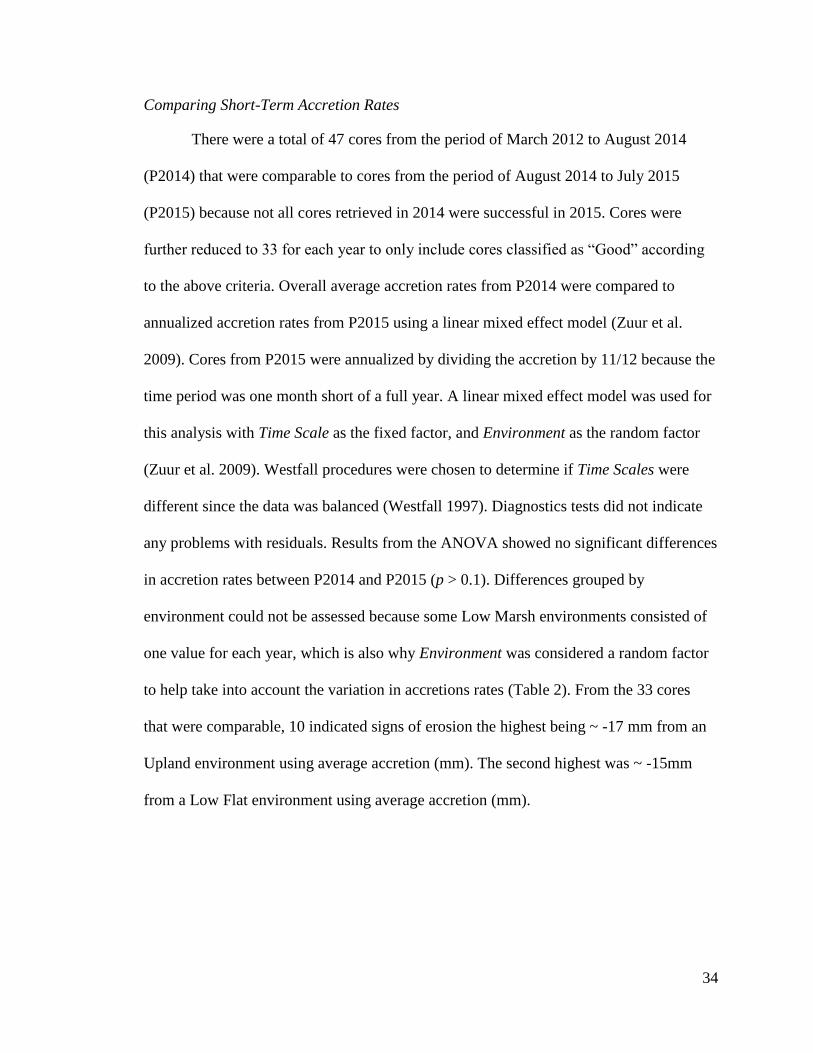
Comparing Short-Term Accretion Rates ...................................................................52

Correlation to Elevation .............................................................................................53

Relative Contribution of Organic and Inorganic Matter ............................................54

Grain Size...................................................................................................................59

Implications for Sea-Level Rise and Marsh Loss ......................................................59

Conclusion .....................................................................................................................62

Chapter 3: Assessing Hydrological Influences ..................................................................63

v

Introduction ....................................................................................................................63

Materials and Methods ...................................................................................................64

Water Level Loggers..................................................................................................64

Sediment Plates ..........................................................................................................72

Sediment Characterization .........................................................................................74

Results ............................................................................................................................74

Hydroperiod ...............................................................................................................74

Grain Size Analysis....................................................................................................82

Discussion ......................................................................................................................85

Influence of Hydroperiod on Deposition ...................................................................86

Contribution of Organic and Inorganic Matter Associated with Hydroperiod ..........88

Grain Size...................................................................................................................90

Sediment Plate Technique ..........................................................................................93

Conclusion .....................................................................................................................94

References ..........................................................................................................................95

vi

List of Figures Fig. 1 Conceptual model of salt marsh responses to sea level rise in terms of sediment supply and

terrestrial slope after Brinson et al. (1995). __________________________________________ 7

Fig. 2 Environmental state changes from upland to open water after Brinson et al. (1995)._____ 8

Fig. 3 Regional map of study area (a), aerial imagery of study site (b). ____________________ 9

Fig. 4 High marsh environment dominated by Monanthochloe litoralis with sparse Salicornia

spp. ________________________________________________________________________ 13

Fig. 5 Transition of environments from high marsh to upland dominated by Spartina patens. _ 14

Fig. 6 Less frequently inundated low marsh environment dominated by Avicennia germinans and

Batis maritima. _______________________________________________________________ 14

Fig. 7 Tidal flats consisting mostly of algal mats in low tidal flat environments. ____________ 15

Fig. 8 Conceptual diagram showing distribution of field methods used in this study. ________ 17

Fig. 9 Creating a horizon marker with a mixture of kaolinite and red brick dust in March 2012. 21

Fig. 10 Horizon marker distribution created in March 2012. ___________________________ 21

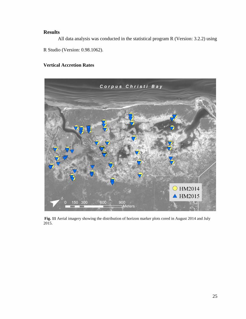
Fig. 11 Aerial imagery showing the distribution of horizon marker plots cored in August 2014

and July 2015. _______________________________________________________________ 25

Fig. 12 Sample core from a horizon marker plot in a high marsh area showing sediment accretion

accumulated from March 2012 to August 2014. Photos from left to right taken from different

angles. _____________________________________________________________________ 26

Fig. 13 Plot showing Accretion Rate for each Environment separated by Time Scale. ________ 28

Fig. 14 Results from ANOVA comparing different Time Scales within specific levels of

Environment. a) High Marsh, b) High Flat, c) Low Marsh, d) Low Flat. Different number of

asterisks between levels indicate significance (p < 0.1). Same number of asterisks between levels

indicate no significance (p > 0.1). ________________________________________________ 30

Fig. 15 Results from ANOVA comparing different Environments within specific Time Scales

using Horizon Markers only; a) Vertical accretion rates for the period of March 2012-August

2014, b) Vertical accretion rates for the period of March 2012-July 2015. Different number of

asterisks between levels indicate significance (p < 0.1). Same number of asterisks between levels

indicate no significance (p > 0.1). ________________________________________________ 31

Fig. 16 Erosion pin heights in all environments throughout the study. ____________________ 33

Fig. 17 Scatterplot showing relationship between accretion and elevation using horizon markers

for the period of Marsh 2012 to August 2014. Plot on the left shows accretions from all

environments. Plot on the right shows accretion data for salt marsh only, low marsh and high

marsh environments. Error bars indicate standard error. _______________________________ 36

Fig. 18 Scatterplot showing relationship between accretion and elevation using horizon markers

for the period of Marsh 2012 to August 2015. Plot on the left shows accretions from all

environments. Plot on the right shows accretion data for salt marsh only, low marsh and high

marsh environments. Error bars indicate standard error. _______________________________ 37

Fig. 19 Scatterplot showing relationship between accretion and elevation using 137

Cs

(Radosavljevic 2011). Plot on the left shows accretions from all environments. Plot on the right

shows accretion data for salt marsh only, low marsh and high marsh environments. Error bars

indicate standard deviation. _____________________________________________________ 38

Fig. 20 Textural classification of sediment samples from horizon markers. a) Horizon markers

cored in August 2014, b) Horizon markers cored in July 2015. _________________________ 40

vii

Fig. 21 Relationship between percent organic matter and Environment for both Time Scales using

horizon markers. _____________________________________________________________ 41

Fig. 22 Relative contributions of organic and inorganic matter to accretion from horizon markers

cored in August 2014 for the period of March 2012 to August 2014. Organic matter contributions

include porosity and water content. Rate of sea level rise at Rockport, TX is also shown by the

light grey area. _______________________________________________________________ 43

Fig. 23 Relative contributions of organic and inorganic matter to accretion from horizon markers

cored in July 2015 for the period of March 2012 to July 2015. Organic matter contributions

include porosity and water content. Rate of sea level rise at Rockport, TX is also shown by the

light grey area. _______________________________________________________________ 44

Fig. 24 Relative contributions of organic and inorganic matter to accretion from 137

Cs cores from

previous study (Radosavljevic 2011). Organic matter contributions includes porosity and water

content. Rate of sea level rise at Rockport, TX is also shown by the light grey area. _________ 45

Fig. 25 Relationship between vertical accretion rates and both organic and inorganic accretion

rates from combined (HM2014 and HM2015) horizon markers (annual time scale) and 137

Cs

(decadal time scale). a) organic accretion b) inorganic accretion c) organic versus inorganic d)

legend for all three graphs. Note: These graphs do not take into account porosity and water

content. _____________________________________________________________________ 46

Fig. 26 Organic and inorganic contributions of HM2014 (top) and HM2015 (bottom) excluding

pore and water space. __________________________________________________________ 51

Fig. 27 Comparison of the relationship of vertical accretion with organic and inorganic accretion

in the present (MUI Horizon Marker) and previous study (MUI 137

Cs) for this area as well as

other localities a) organic accretion, b) inorganic accretion, c) organic versus inorganic accretion,

d) legend for all plots indicating locations. Data of other studies are from Turner et al. (2002) for

Upper Texas coast, Louisiana, and Rhode Island, and data for Texas (Aransas National Wildlife

Refuge), San Bernard, Mississippi, and Florida Keys are from Callaway et al. (1997). _______ 56

Fig. 28 A comparison of the relationship between organic accretion and inorganic accretion. a)

This study combined with Radosavljevic (2011), b) Louisiana studies from Fig. 20. Shaded

regions indicate 95% confidence interval. This figure is the similar to Fig. 20c except the

geographic localities are plotted separately for visualization. ___________________________ 58

Fig. 29 Range of elevations for each environment. Low flat elevations vary in this area, but are

generally considered to be at lower elevations than low marsh environments. ______________ 60

Fig. 30 Map showing wetland transitions from 1950’s, 1979, and 2002-04 for Mustang Island and

Harbor Island (White et al. 2006). Study area in Mustang Island is highlighted by the red box. 61

Fig. 31 Distribution of water levels loggers on Mustang Island, TX. _____________________ 65

Fig. 32 OTT Orpheus mini water level logger suspension diagram (Source: OTT Orpheus Mini

2015). ______________________________________________________________________ 66

Fig. 33 HOBO Onset water level logger deployment diagram (Source: HOBO Onset 2015). __ 67

Fig. 34 Schematic of hydroperiod measurements at sediment plates using nearest water level

logger. _____________________________________________________________________ 71

Fig. 35 Example of how number of flooding events were counted. F1 indicates 1st count of

flooding event, and continues to F4, so in this example Number of Flooding Events = 4 (number

of time sediment plate was exposed after initial flooding event). ________________________ 71

viii

Fig. 36 Circular sediment plate modeled after Kleiss (1993). Diagram of sediment plate (left),

sediment plate example from low marsh environment after flooding event (right). __________ 72

Fig. 37 Sediment plate distribution on Mustang Island, TX. ____________________________ 73

Fig. 38 Relationship of sediment plate deposition with flooding duration in time and depth. a) all

sediment plates, b) only sediment plates that were flooded, c) all sediment plates with y-axis log

scaled, d) only flooded sediment plates with y-axis log-scaled. _________________________ 77

Fig. 39 Relationship of sediment plate deposition with number of flooding events (a) and duration

in time and depth (b) for plates in low marsh environments near the main tidal creek only. ___ 78

Fig. 40 Relationship between accumulation of both organic and inorganic matter with duration in

time and depth. Accumulation of matter does not take into account sediment porosity, density or

water content. ________________________________________________________________ 80

Fig. 41 Water level referenced to NAVD88 near main tidal creek, including sediment plate

elevations. Horizontal lines represent elevation of sediment plates on the marsh surface. _____ 81

Fig. 42 Sediment grain size for all sediment plates, excludes plates with bioturbation. a) grain size

classified by vegetation type, b) grain size classified by range of elevation. _______________ 83

Fig. 43 Sediment grain size for plates near the main tidal creek, excludes plates with bioturbation.

a) grain size classified by sediment plate ID, b) grain size classified by vegetation type. _____ 84

Fig. 44 Precipitation and wind direction and magnitude throughout the study period. Y-axis

represents precipitation in centimeters. Stick plot shows wind direction and magnitude (scaled

relatively to each other). Winds pointing north (90˚) indicate winds are coming from the south

headed north _________________________________________________________________ 87

Fig. 45 A comparison of the relationship between accumulation of both organic and inorganic

matter and duration of flooding (log10 scaled x-axis) in the present study, using sediment plates

near the main tidal creek, and in a study in Louisiana. ________________________________ 89

Fig. 46 Mean grain size analysis and skewness from Simms et al., (2006) and Radosavljevic,

(2011). _____________________________________________________________________ 92

Fig. 47 Mean grain size analysis and skewness for this study. __________________________ 93

List of Tables Table 1 Comparison of accretion rates using different time scales averaged by wetland

classifications. ................................................................................................................................ 27

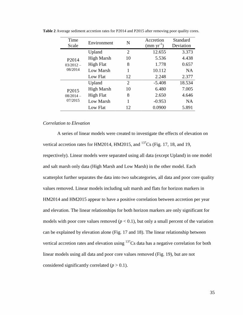
Table 2 Average sediment accretion rates for P2014 and P2015 after removing poor quality

cores. .............................................................................................................................................. 35

Table 3 List of hurricanes, tropical storms depression since 1963 within 200 km of Mustang

Island (NOAA, 2014b)................................................................................................................... 49

ix

Acknowledgments

First and foremost, I would like to thank my committee members: Dr. James C.

Gibeaut, Dr. Michael Starek, and Dr. Mark Besonen for their insight and expertise

throughout my thesis project, especially my advisor, Dr. Gibeaut for providing me the

opportunity to work in the Coastal and Marine Geospatial Lab (CMGL). I would like to

thank everyone in the CMGL for their help and guidance, especially a huge thank you to

Marissa Dotson for helping me out in the field. I would also like to thank everyone who

helped me install water level loggers and carry heavy fence posts during the Texas heat in

July 2014, as part of the National Oceanic and Atmospheric Administration

Environmental Cooperative Science Center (NOAA ECSC) Field Campaign. I would like

to thank the NOAA ECSC, for not only supporting this project (NA11SEC4810001), but

providing me with several opportunities for training, networking, and travel to

conferences and working offshore on the E/V Nautilus. I would also like to thank Alan

Downey-Wall for all of his support throughout my graduate career and for going into the

field with me when no one else could, especially for his help in retrieving water level

loggers during the coldest times of the year. I would also like to thank Harte Research

Institute, especially Gail Sutton for allowing me to borrow the truck every other week,

and Mike Grubbs for helping me schedule vehicle use, and teaching me how to use power

tools. Lastly but not least, I would like to thank the many friends I have made here, and

my family for all of their never-ending support, inspiration, and encouragement. I have

learned so much as a graduate student and plan on building on the skills I have acquired

here throughout my career. Thank you!

x

“There is no other case in nature, save in the coral reefs, where the adjustment of

organic relations to physical conditions is seen in such as beautiful way as the balance

between the growing marshes and the tidal streams by which they are at once nourished

and worn away.” (Shaler 1886)

1

Chapter 1: Introduction

Importance of Texas Estuarine Wetlands

Wetlands areas are known to have high biological productivity and diversity, but

recently there has been an increase in awareness of the critical role coastal wetlands play

and the need to monitor the status and trend as sea level rises (White et al. 2006).

Effective management of the structure and functions of coastal wetlands is necessary to

protect wetlands’ many contributions to ecosystem goods and services. According to

Costanza et al. (1997) the value of tidal marsh wetlands worldwide is estimated around

$1.6 trillion per year from waste treatment, habitat and refuge, food production, raw

materials, and recreation values. Aesthetic appreciation and spiritual values are often

strong motivators for action, but the most difficult to assign monetary values. Salt

marshes also serve to maintain fisheries by boosting the production of economically

important fishery species such as shrimp, oysters, clams, and various commercial fish. In

the Gulf of Mexico, salt marshes account for as much as 66% of the shrimp and 25% of

the nation’s blue crab production (Barbier et al. 2010). In 2012, U.S. commercial and

recreational fishing industries in Texas generated about $4.2 billion in sales, employing

about 40,000 coastal residents (NOAA 2012). Salt marshes provide nursery grounds for

juvenile fish, shrimp, and shellfish because of the complex packed plant structure

inaccessible to larger fish. Salt marshes sequester millions of carbon annually generated

by biochemical activity, sedimentation, and biological productivity. Other benefits from

salt marshes include erosion control by providing sediment stabilization and soil retention

in vegetation root structure; water purification by providing nutrient uptake, retention,

and deposition; raw materials and foods generated by biological productivity and

2

diversity; and tourism, recreation, education, and research by providing a unique and

aesthetic landscape, and a suitable habitat for diverse fauna and flora (Costanza et al.

1997; Barbier et al. 2010).

The loss and degradation of wetlands can be attributed to indirect influences such

as population growth and economic development, and direct influences such as

infrastructure development, land conversion, water withdrawal, pollution, overharvesting

and overexploitation, and introduction of invasive species (Finlayson et al. 2005). The

effects of climate change, such as sea level rise as well as changes in hydrology and

temperature, will lead to reduction in services provided by wetlands which could result in

erosion of shores and habitat, altered tidal ranges in rivers and bays, changes in sediment

and nutrient transport, and increased coastal flooding (Finlayson et al. 2005). Wetlands

are highly valued due to their ability to protect the coast by providing a buffer against

these climate change impacts.

Wetland Sedimentation: General Overview

There is growing concern as to whether salt marsh wetlands can withstand the

accelerated rise in sea level by vertically accreting. There are two ways in which marshes

may be submerged, either sea level rises or the land subsides, or a combination of both.

Subsidence measurements focus on changing land surface elevation relative to a specific

datum. The term shallow subsidence, which is calculated as the difference between

vertical accretion and elevation change, is often differentiated from the term deep

subsidence, which includes additional compaction and biostatic processes (D.R. Cahoon

et al. 1995; Donald R. Cahoon et al. 2006). Shallow subsidence consists of subsurface

processes near the marsh surface, such as compaction, decomposition, and dewatering

3

(Donald R. Cahoon and Lynch 1997). Deep subsidence occurs in all marshes from

sinking of soil due to compaction and other geological processes, but can vary greatly

between different locations due to human influences. This is the case for marshes along

the Texas coast with higher deep subsidence rates near Galveston, TX (White et al.

2001). Deep subsidence rates have been measured as high as 70 mm yr-1

over the Saxet

Oil and Gas field in Corpus Christi, TX and 75 mm yr-1

in the Houston, TX area near the

heart of the “subsidence bowl” (Pulich et al. 1997). Natural compaction processes have

been accelerated in many areas due to withdrawal of subsurface fluids, such as water, oil,

and gas (White et al. 2001).

Subsidence can occur in conjunction with accretion. Although a marsh with high

sedimentation rates may build vertically, high rates of subsidence can create an accretion

deficit. The deficit is calculated by comparing measures of accretion or accumulation

with estimates of sea level rise or land subsidence (Reed and Cahoon 1993). Marshes can

build vertically to overcome the effects of sea level rise by mineral sediment deposition

and accumulation of plant roots and decaying plant material (organic matter), which are

controlled by hydrological processes (Reed and Cahoon 1992). Flooding patterns control

the delivery of sediment and oxygen content of the soil which influences the rate of

growth and decay of plants (Reed and Cahoon 1992; D.R. Cahoon 1997). Vegetation also

enhances sediment deposition by slowing down the current and trapping suspended

sediment. Accretion in marshes remote from riverine sources of sediment may occur

through resuspension of sediment from bay bottoms and deposition on adjacent marshes

(D. R. Cahoon and Reed 1995). Key factors affecting sedimentation include bioturbation,

4

current intensity, channel migration, vegetation cover, and location. Organic matter

accumulation is often more important than inorganic matter in deteriorating marshes.

Seasonal sedimentation patterns are associated with the passage of winter cold fronts

along the northwestern Gulf of Mexico coast (Reed 1989). Inorganic sediment can be

deposited when the marsh is flooded due to storm surge, but the amount of sediment

contribution varies (Reed 1989). During storms, washover fans serve as a source of

sediment, transporting sediments from the ocean side for eventual deposition in the

marshes.

Strong winds preceding a cold front also plays an important role across the marsh

causing water levels to rise by wave action, which in turn floods the marsh mobilizing the

sediment and depositing it on the surface. Winds after the cold front depress water levels

which allows the newly deposited sediments to drain and begin to consolidate (Reed

1989). Storms (cold fronts) and summer tropical cyclones (hurricanes) are often the main

mechanism for mobilizing sediment for marshes that are remote from a riverine sediment

source and help maintain marshes stable against sea-level rise effects (Stumpf 1983; Reed

1989; D. R. Cahoon and Reed 1995).

Wetlands Response to Sea Level Rise

The interaction between hydrodynamics and elevation create a shore-parallel

zonation of vegetation, which becomes increasingly complex due to the

micromorphology of the marsh surface. The salinity of the water controls the

composition of the vegetation and fauna, which help to characterize the marsh. Previous

studies have shown that species competition is also critically important in controlling the

salt marsh plant communities (Bertness 1991). The existence and type of estuarine

5

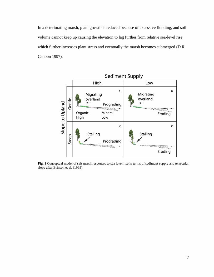
wetlands are closely controlled by their position in the tidal frame. In absence of human

development as sea level rises and the tidal frame shifts, wetlands generally follow a

pattern of either migrating over land or stalling at the terrestrial-marsh margin and either

prograding or eroding at the seaward margin as shown by Fig. 1 (Brinson et al. 1995).

These patterns are strongly influenced by the amount of sediment brought into the

system, the steepness of the slope from upland to open water, and the relative sea level

rise rate, which includes eustatic sea level rise plus subsidence rates (Fig. 1). Migration

overland can sometimes be halted by a steep slope or human infrastructure.

Brinson et al. (1995) described how disturbances to wetlands, such as sea level rise,

can alter the ecosystem and cause a change in state depending on the frequency and

degree of the disturbance (Fig. 2). The chronic and gradual change of sea level leads to

higher frequency and pulsing that ultimately changes ecosystem states (Brinson et al.

1995). Ecosystem states transform from one class to another if the hydrology and

sediments have been changed drastically. If not, the vegetation proceeding the

disturbance remains the same, as conceptualized by Fig. 2 (Brinson et al. 1995).

Brinson’s state changes can follow the transitions from upland to high marsh, high

marsh to low marsh, low marsh to subtidal environment, or subtidal environment to open

water. Each state is characterized by inundation frequency, sediment dynamics, pore

water salinities, plant communities, and species composition (Brinson et al. 1995). The

lower limit of the marsh, which is defined as the seaward margin, is regularly inundated

by salt water and consists of pioneer species such as Spartina alterniflora. At higher

elevations - mid-level salt marsh - the hydroperiod is less frequent, therefore a greater

diversity of plant species are able to colonize. Salt tolerant plant species do not occur in

6

non-saline environments because they are unable to compete with non-salt tolerant plant

species.

If the rise in sea level is not equivalent to vertical accretion of marsh sediments,

then there will be a gradual disintegration of coastal marshes due to increased inundation,

erosion, and saltwater intrusion (Mitsch and Gosselink 2000). Disturbance in the higher

elevated areas, such as the upland and high marsh areas, are mostly caused by saltwater

intrusion for prolonged periods of time causing non-salt tolerant plant species to die off

(Fig. 2). Disturbance in the lower elevation areas is mostly caused by redistribution of

sediments. The transition of a state could also be reversed for continuously prograding

marshes. The reversal of a state is the difference between prograding and eroding at the

seaward margin (Brinson et al. 1995).

Each state has self-maintained processes that resists change by accumulation of

organic and inorganic matter as a way to increase elevation to overcome relative sea-level

rise (Brinson et al. 1995). As the elevation increases by sediment accretion, the

hydroperiod and net sediment accretion are reduced, thus causing a change in state.

Changes in elevation can be due to vertical accretion or changes in the volume of soil

related to subsurface processes (D.R. Cahoon et al. 1995). Erosion and accretion can be

significant in some areas, therefore, vertical accretion rates on wetland surfaces may

offset sea level rise in areas of high accretion rates while in other areas erosion may

exacerbate wetland loss as sea level rises (Gibeaut et al. 2010). Wetland migration is

critical for areas where vertical and horizontal accretion rates are not sufficient to offset

sea level rise. A marsh is considered healthy if the marsh elevation increases at the same

rate as the sea-level rises and flooding patterns remain unchanged (D.R. Cahoon 1997).

7

In a deteriorating marsh, plant growth is reduced because of excessive flooding, and soil

volume cannot keep up causing the elevation to lag further from relative sea-level rise

which further increases plant stress and eventually the marsh becomes submerged (D.R.

Cahoon 1997).

Fig. 1 Conceptual model of salt marsh responses to sea level rise in terms of sediment supply and terrestrial

slope after Brinson et al. (1995).

8

Fig. 2 Environmental state changes from upland to open water after Brinson et al. (1995).

9

Study Area

Fig. 3 Regional map of study area (a), aerial imagery of study site (b).

10

This study seeks to investigate accretion rates at short, medium, and long-term

scales to determine the status of the marsh relative to local sea level rise. This study was

conducted on the bay side of the Texas barrier island known as Mustang Island (Fig. 3).

There have been many studies conducted on Mustang Island including the assessment of

medium-term vertical accretion rates determined from radiometric dating methods

(Radosavljevic 2011). Radosavljevic (2011) determined vertical accretion rates from 13

shallow sediment cores taken in high marsh, high flat, low marsh, and low flat

environments. The area is also near a deep set survey benchmark to reference elevation,

and has a continuously monitored elevation transect that runs from the middle of the

barrier island to the bay shoreline surveyed by a Trimble Total Station and Real Time

Kinematic Global Positioning System (RTK GPS). The location is considered the

Mustang Island Wetland Observatory by the Harte Research Institute for Gulf of Mexico

Studies due to the extensive research of the area.

Mustang Island is a bay mouth barrier island located along the southern portion of

the Texas Gulf Coast bound by Corpus Christi Bay, the Laguna Madre, and the Gulf of

Mexico. Mustang Island lies above the ancestral Nueces River valley and its tributaries,

and the Pleistocene surface beneath reaches depths as great as 38 m (Simms et al. 2006).

This suggests that sea level transgressed the area earlier than other Texas coastal

locations, thus making Mustang Island older than other modern barrier islands on the

Texas coast (Simms et al. 2006). The rise and fall of sea level during the Pleistocene

Epoch resulted in the formation of large sand bars along the coastline that developed into

barrier islands over time (Moulton and Jacob 2000). The Texas mainland shore, coastal

plain, beaches, barrier islands and peninsulas, river deltas, and bays and estuaries are all

11

products of alluvial sediments deposited during the Holocene, the last 10,000 years

(Moulton and Jacob 2000).

Texas barrier beaches are generally composed of well-sorted fine to very fine sand

(Morton 1988). Estuarine wetland soils can range from clay to sand, but fine sand

dominates most barrier island salt marshes in Texas. Winds strongly influence coastal

geoenvironments along the semi-arid Texas coast. Onshore southeasterly winds are

consistent during most of the year but are periodically directed offshore by strong

northerly winds associated with cold fronts during winter months (White et al. 1978;

Shideler 1984). Mustang Island is considered a high-profile barrier generally considered

older and more stable, which results in less material delivered to the backbarrier

environment due to the high amount of sediment trapped by the dunes (Simms et al.

2006).

Mustang Island lies in the Texas Coastal Bend at the approximate boundary where

precipitation exceeds evaporation to the north and evaporation exceeds precipitation to

the south (Montagna et al. 2007). Precipitation and evaporation are important for

sediment accretion and deposition due to their influence on vegetation and soil moisture.

There is a general climatic gradient southwestward along the Texas coast decreasing in

precipitation, sedimentation, distribution of wetlands, and subsidence, and increasing in

active dunes correlated with diminishing vegetation cover (White et al. 2001). The

arcuate shape of the Texas coast causes longshore current northeast to flow southwest

and longshore currents in the south to flow north, converging at the coastal bend.

Astronomical tides in this region of the Gulf of Mexico are generally considered

diurnal or mixed ranging from 45 to 60 cm; these tidal variations are even lower in the

12

bays (Morton and McGowen 1980). Tidal range on the Gulf side of Mustang Island is

0.60 m, while on the bay side of Mustang Island tidal range is about 0.10 m, although

tides in the bays can be wind-generated (White et al. 1978; Montagna et al. 2007). The

area is characterized as a microtidal wave-dominant coast subject to diurnal tides (Morton

1988). Mean significant wave height is 1.4 m while wave breaker heights along the Gulf

shore are generally less than 1.2 m with an average breaker height being slightly more

than 0.6 m (White et al. 1978; Gibeaut et al. 2008). Microtidal coasts are generally storm

dominant coasts because the energy and geological change during storms are far greater

than changes that occur by daily processes (Morton and McGowen 1980).

Microtidal marshes are more vulnerable to rapid sea level rise because the amount

of rise is a larger percentage of the tide range to which marshes are adjusted compared to

meso or macrotidal range settings. A rise of just 0.1 m in relative sea level along the

Texas coast can cause conversion of fringing low marshes and flats to open water and sea

grass beds, and usually dry high marshes and flats to usually wet low marshes and flats

(Stevenson et al. 1985; Gibeaut et al. 2003). Tide gauge records from Rockport, TX,

located near Mustang Island, indicate a relative mean sea-level rise rate of 5.27 ± 0.48

mm from 1937 to 2014 (NOAA 2014a). Land subsidence rates on the south Texas barrier

islands were calculated to be approximately 1 to 5 mm yr-1

(Montagna et al. 2007). In

general, areas with thicker and rapidly deposited Holocene sediment have a higher

compaction rate. The sediment deficit and low-lying gently sloped shores of much of

south Texas coast will cause relative sea-level rise to have a profound effect on coastal

habitats (Montagna et al. 2007).

Environments

High Marsh and Upland

13

High marsh environments vary in range from 0.2 – 0.8 m (NAVD88) well above

the mean high tide line therefore are rarely inundated by tides (Paine, White, Gibeaut, et

al. 2004). At lower elevations within the high marsh range, Monanthochloe litoralis

(shoregrass) is the dominant species commonly found growing in mats (Fig. 4).

Occasionally there is sparse Salicornia spp. (glasswort), but presence varies seasonally.

Other species commonly found in high marsh environments include Batis maritima

(pickleweed), Salicornia spp. (glasswort), and Lycium carolinianum (Carolina

wolfberry). At higher elevations as high marsh transitions to upland environments

Borrichia frustescens (sea ox eye daisy) and Distichlis spicata (seashore saltgrass)

dominate. For this study environments containing Spartina patens (salt hay grass) and

Spartina spartinae (gulf cordgrass), which lie just above high marsh environments, were

classified as upland (Fig. 5). Upland environments range in elevation from 0.52 – 5.49 m

(NAVD88) (Paine, White, Smyth, et al. 2004).

Fig. 4 High marsh environment dominated by Monanthochloe litoralis with sparse Salicornia spp.

14

Fig. 5 Transition of environments from high marsh to upland dominated by Spartina patens.

Low Marsh

Low marsh areas are very high in biologic productivity usually ranging in

elevation from -0.1 – 0.3 m (NAVD88) (Paine, White, Gibeaut, et al. 2004). More

frequently inundated areas near tidal creeks are dominated by S. alterniflora (smooth

cordgrass), with Avicennia germinans (black mangrove) and B. maritima following,

whereas less frequently inundated low marsh environments are dominated by B. maritima

and A. germinans (Fig. 6). Historically A. germinans were restricted to the south by

winter freezes, but there has been noticeable expansion northward into S. alterniflora salt

marshes.

Fig. 6 Less frequently inundated low marsh environment dominated by Avicennia germinans and Batis

maritima.

15

Tidal Flats

Tidal flats are extensive on Mustang Island ranging in elevation from -0.05 to 0.5

m (NAVD88) (Paine, White, Gibeaut, et al. 2004). Low regularly flooded tidal/algal flats

are slightly more abundant than high flats (Fig. 7). Tidal flats in this area are designated

as wind-tidal flats because many of the flats are flooded only by wind-driven tides (White

et al. 2006). Blue-green algae flourish in low tidal flats after long periods of inundation,

producing thick mats which bind fine sediment. Some algal flats are characterized as

having a spongecake texture (White et al. 1978). In some areas salt marsh vegetation such

as M. litoralis, B. maritima, and Salicornia spp. can be found sparingly.

Fig. 7 Tidal flats consisting mostly of algal mats in low tidal flat environments.

General Purpose

It is important to quantify sedimentation rates to understand changes due to

hydrology and biologic processes and how the rates of sediment accretion affect the

ability of plants to adapt to the variation of water level. Previous sea level rise models

have shown an upland transition of wetlands while the low marsh environments decrease

drastically in the backbarrier estuarine wetlands of Mustang Island (Gibeaut 2007).

Marshes can potentially overcome sea level rise by accretion of organic and inorganic

16

matter or landward migration. Currently medium-term (50 years) accretion rates have

been calculated for Mustang Island (Radosavljevic 2011), but information on short-term

accretion rates has not been assessed.

Short-term studies generally highlight spatial and temporal variations with phases

of deposition interrupted by erosion, which can be useful in determining migration,

erosion and deposition rates in salt marshes (D.R. Cahoon and Turner 1989). Shorter term

perspective becomes increasingly relevant in an environment impacted by climate

change, change of land use, or other human activities (Blake et al. 1999). Examining

sedimentation rates over a range of time scales provides insight into the factors that

control marsh elevation and sedimentation processes (Neubauer et al. 2002). Because of

the relationship between elevation, vegetation, and tidal inundation, wetland accretion is

expected to vary for different wetland environments in the study area. Erosion processes

are more likely to occur in sparsely vegetated parts of the marsh, such as the pioneer zone

(Nolte et al. 2012). Thus, measuring short-term (1 to 3 years) accretion amounts could be

used to assess vegetation-sedimentation interactions. Additionally, water level loggers

were used in this study near sediment accretion measurement points as a way to assess

how hydrology influences sediment accretion rates on a short-term scale. An overview of

the methods used for this study is shown in Fig. 8.

Using this approach, we are able to learn more about current processes affecting

sedimentation rates and determine how accretion rates affect modern wetland

sustainability. Results from this project will help determine the relative importance of

elevation, inundation, vegetation type, and other geospatial and biophysical influences on

sediment accretion. There is a fundamental need to understand vertical accretion, and the

17

associated sediment dynamics in salt marsh ecosystems. This research seeks to contribute

to the fields of coastal research by providing modern accretion rates and assess the major

influences that could possibly be used to improve models used to help predict

evolutionary changes of coastal wetlands, such as the Sea-Level Affecting Marshes

Model (SLAMM).

Fig. 8 Conceptual diagram showing distribution of field methods used in this study.

18

Chapter 2: Assessing Sediment Accretion Rates

Introduction

As sea level rises there is a growing concern about the ability of wetland

environments to survive. Vertical accretion of sediment in salt marshes is one of the

fundamental processes determining a wetlands ability to overcome accelerating sea level

rise rates. Wetlands can either migrate landward or accrete vertically as sea level rises

depending on the amount of sediment supply and slope to upland regions (Brinson et al.

1995). Vertical accretion is influenced by many factors such as availability of organic and

inorganic matter, vegetation, species composition, flooding patterns, elevation, storm

activity, sediment compaction, wind speed and direction, and relative sea-level rise

(Cahoon and Turner, 1989; Goodman et al., 2007; Gosselink and Turner, 1978). Vertical

accretion rates are commonly compared to relative sea-level rise rates to determine future

wetland stability.

Many methods measuring vertical accretion for different time scales have been

used throughout the scientific community (Thomas and Ridd 2004; Nolte et al. 2012).

The purpose of this thesis is to determine the nature of sedimentation on the coastal

fringing salt marsh of Mustang Island, TX by a combination of erosion pins, kaolinite

marker horizons, and Cs-137 measurements acquired by Radosavljevic (2011). Cesium-

137 profiles yield accretion rates on the decadal scale, whereas as marker horizons

determine annual accretion rates, and erosion pins determine biweekly rates. A

combination of methods across different time scales has been known to reduce error

19

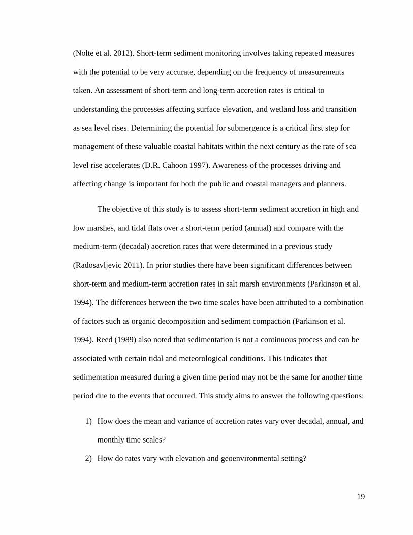
(Nolte et al. 2012). Short-term sediment monitoring involves taking repeated measures

with the potential to be very accurate, depending on the frequency of measurements

taken. An assessment of short-term and long-term accretion rates is critical to

understanding the processes affecting surface elevation, and wetland loss and transition

as sea level rises. Determining the potential for submergence is a critical first step for

management of these valuable coastal habitats within the next century as the rate of sea

level rise accelerates (D.R. Cahoon 1997). Awareness of the processes driving and

affecting change is important for both the public and coastal managers and planners.

The objective of this study is to assess short-term sediment accretion in high and

low marshes, and tidal flats over a short-term period (annual) and compare with the

medium-term (decadal) accretion rates that were determined in a previous study

(Radosavljevic 2011). In prior studies there have been significant differences between

short-term and medium-term accretion rates in salt marsh environments (Parkinson et al.

1994). The differences between the two time scales have been attributed to a combination

of factors such as organic decomposition and sediment compaction (Parkinson et al.

1994). Reed (1989) also noted that sedimentation is not a continuous process and can be

associated with certain tidal and meteorological conditions. This indicates that

sedimentation measured during a given time period may not be the same for another time

period due to the events that occurred. This study aims to answer the following questions:

1) How does the mean and variance of accretion rates vary over decadal, annual, and

monthly time scales?

2) How do rates vary with elevation and geoenvironmental setting?

20

3) How much organic and inorganic matter is associated with the accreted

sediments?

Ultimately, this information will contribute to our understanding of sedimentation in a

sandy, semiarid, microtidal environment.

Material and Methods

A combination of different methods was used to measure sedimentation rates in a

barrier island, brackish salt marsh (Fig. 8).

Sedimentation measurements

(1) Horizon Marker: In March 2012, 166 sites within Mustang Island were

selected for emplacement of kaolinite and red brick dust. The kaolinite and brick dust

mix material was spread out on the marsh floor within a 44 x 44 cm quadrant (Fig. 9).

RTK GPS measuring x, y, z coordinates were taken at each marker as well as two PVC

stakes placed at opposite corners of the quadrant to facilitate finding the plots. Plots were

spatially distributed across the study area in different patterns (Fig. 10). Some plots

followed a transect perpendicular to the barrier island to analyze how accretion varied

with distance to water ways, while other plots were grouped to surround a specific

environment for detailed monitoring. The grouped plots consisted mostly of low marsh

environments since in those settings there was difficulty assessing accretion rates using

the 137

Cs technique previously (Radosavljevic 2011).

21

Fig. 9 Creating a horizon marker with a mixture of kaolinite and red brick dust in March 2012.

Fig. 10 Horizon marker distribution created in March 2012.

22

In August 2014 and July 2015, small, clear tubes 2.5 cm in diameter and 1.5 mm

thin were used to core each horizon marker plot. The driving ends of the tubes were

beveled to reduce friction. The area cored within the plot was replaced by sediment

adjacent to the area and was recorded for future investigation. Two additional cores of the

top 2 cm were taken adjacent to the horizon marker plot for grain size analysis, and

analysis of organic and inorganic content. Using a micromillimeter caliper, four

measurements, evenly spaced around the core tube, were recorded to measure the

accretion above the horizon marker. For cores taken in August 2014, the average

accretion was divided by years for the period of March 2012 to August 2014. For cores

taken in July 2015, the average accretion rate was divided by years for the period of

March 2012 to July 2015. The average accretion rates from August 2014 to July 2015

were also assessed. Vertical accretion is defined as a gross linear sediment accumulation.

There are several advantages of using the horizon marker methodology: it is low

cost; it can be used in vegetated areas; core measurements are simple and fast;

measurements are not influenced by interference of the measuring equipment; and it

measures both organic and inorganic accumulation. Disadvantages include loss of

markers by bioturbation or erosion associated with flood events.

(2) Erosion Pins: Erosion pins (30-pins) made of stainless steel 1.5 mm in

diameter 1 m in length were installed approximately 3 inches northeast of each sediment

plate also installed for this study. Erosion pins were distributed in high marsh, low marsh

and tidal flat environments, upland environments were not included. The pins were

driven into the ground leaving a small portion aboveground for measurement. The height

of the pin was measured every two weeks when sediment plates were retrieved.

23

Measurement for each erosion pin was repeatedly made from the same angle to reduce

error. The measurement error associated with this method is about 1 mm (Nolte et al.

2012). Biweekly rates from erosion pins were annualized for comparisons by summing

the biweekly rates throughout the year for each pin, and then averaging by environment.

Collecting accretion/erosion from erosion pins allows more frequent sampling,

and avoids the problem of sediment compaction, and has the ability to capture temporal

and spatial episodic events. Frequent observation also gives a more detailed indication of

variations in seasonal-related marsh sedimentation processes than is available from

marker horizons.

(3) 137Cs:

137Cs is an anthropogenic radioisotope with a half-life of 30.17 years.

The radioisotope was introduced into the environment during the 1950’s and 60’s during

atomic nuclear testing. Concentration of 137

Cs usually reveals a strong spike in 1963

when atmospheric atomic testing was at its highest. Vertical accretion rates are

commonly assessed using the 1963 spike as a dating marker. Accretion rates determined

using radiometric dating methods for Mustang Island, TX were acquired from a previous

study by Radosavljevic (2011).

Sediment Characterization

Organic Matter Content

Organic matter has been shown in many studies to be a significant contributing

factor for accretion rates in salt marshes throughout the Gulf of Mexico (Turner et al.

2002). Following the methods of Turner et al. (2002) the organic matter content of the

soil was determined by loss-on-ignition (LOI). Homogenized samples were placed on a

24

clean crucible and weighed after drying at 60˚C for 24 hours. Sample weights were

determined using an analytical balance. Samples were then burned at 550˚C for 3 hours,

and then reweighed after cooling to calculate percent of organic matter following the

equation:

% 𝑂𝑟𝑔𝑎𝑛𝑖𝑐 =𝑆𝑎𝑚𝑝𝑙𝑒 𝑊𝑒𝑖𝑔ℎ𝑡𝑑𝑟𝑦 − 𝑆𝑎𝑚𝑝𝑙𝑒 𝑊𝑒𝑖𝑔ℎ𝑡𝑎𝑠ℎ𝑒𝑑

𝑆𝑎𝑚𝑝𝑙𝑒 𝑊𝑒𝑖𝑔ℎ𝑡𝑑𝑟𝑦× 100

Grain Size

Sediment samples were initially digested in 5% H2O2 and gradually increased to

10%, 20%, and 30% H2O2 to remove organic matter. Vegetation was removed using

forceps prior to digestion. For sediment samples that did not have sufficient sediment for

analysis of organic matter and grain size an alternate method was chosen. Alternate

method: Grain size analysis was measured after organic material was measured and

removed from the sample using LOI methods. Samples that were burned for organic

matter and reused for grain size were placed in an ultrasonic water bath for one hour to

help separate sediment particles. Grain size was analyzed using a Coulter LS 13 320 laser

particle counter. The Coulter LS 13 320 laser particle counter uses polarized intensity

differential scattering and the tornado dry power dispersing system to produce reliable

particle size analysis without the risk of missing either the largest or smallest particles in

a sample. Maximum particle size for the laser particle analyzer is 2 mm while the

minimum particle size is 0.004 mm. Grain size was represented using the phi scale,

devised by Krumbein, which is a more convenient way of presenting data (Folk 1974).

Each sample was analyzed three times if possible to avoid bias from skewed runs.

Samples were classified in a ternary diagram following Shepard (1954) using the

statistical program R.

25

Results

All data analysis was conducted in the statistical program R (Version: 3.2.2) using

R Studio (Version: 0.98.1062).

Vertical Accretion Rates

Fig. 11 Aerial imagery showing the distribution of horizon marker plots cored in August 2014 and July

2015.

26

Fig. 12 Sample core from a horizon marker plot in a high marsh area showing sediment accretion

accumulated from March 2012 to August 2014. Photos from left to right taken from different angles.

Of the 166 horizon marker plots created in March 2012, 50 plots were

successfully retrieved in August 2014, while 69 plots were successfully retrieved in July

2015 (Fig. 11). Success of a core was determined by the following criteria:

1. Red horizon marker was clearly visible

2. Marker was not smeared from top to bottom

3. Two or more readings were measureable

An example of a successful core is shown by Fig. 12. Accretion was calculated as

follows:

𝐴𝑐𝑐𝑟𝑒𝑡𝑖𝑜𝑛 𝑅𝑎𝑡𝑒 (𝑚𝑚 𝑦𝑟−1) =𝐷𝑒𝑝𝑡ℎ 𝑡𝑜 𝑀𝑎𝑟𝑘𝑒𝑟

𝑌𝑒𝑎𝑟𝑠 𝑆𝑖𝑛𝑐𝑒 𝑀𝑎𝑟𝑐ℎ 2012

For horizon markers cored in August 2014 for the period of March 2012 – August

2014 (HM 2014), depth was divided by 2.416 years. For horizon markers cored in July

2015 for the period of March 2012 – July 2015 (HM 2015), depth was divided by 3.333

years. Average vertical accretion rates are shown in Table 1 for all time scales.

27

Table 1 Comparison of accretion rates using different time scales averaged by wetland classifications.

Time

Scale Environment N

Accretion

(mm yr-1

)

Standard

Deviation

137Cs

1963-2011

High Marsh 6 1.385 0.402

High Flat 3 0.933 0.482

Low Marsh 3 3.263 0.768

Low Flat 1 1.850 NA

HM2014 03/2012-

08/2014

Upland 6 8.574 5.178

High Marsh 13 4.812 3.733

High Flat 13 2.851 2.639

Low Marsh 5 11.056 2.871

Low Flat 13 2.088 2.226

HM2015 03/2012-

07/2015

Upland 13 7.726 5.243

High Marsh 19 4.198 3.543

High Flat 14 3.873 4.504

Low Marsh 8 12.797 5.533

Low Flat 15 1.673 1.145

Erosion

Pin 07/2014-

07/2015

High Marsh 11 6.636 8.834

High Flat 3 -3.333 10.115

Low Marsh 9 16.000 16.598

Low Flat 7 1.714 2.870

Comparing Accretion Rates across All Time Scales

Significant differences showed up at a glance by observing the means and

variation for each environment and time scale (Fig. 13). If the interaction is not

significant you can see roughly parallel lines for any level of a factor. Significant

differences were found between Environment and Accretion Rate for all Timescales (p <

0.1).

A two-way Analysis of Variance (ANOVA) was used to determine the

differences between accretion rates and the four different time scales (137

Cs, HM 2014,

HM 2015, and Erosion Pins). Both Environment and Time Scale were considered fixed

factors in the model. A summary of the ANOVA model gave a general overview of the

significance, indicating Time Scales were significantly different using α = 0.1. 137

Cs

28

timescale was significantly different from HM2014, HM2015, and Erosion Pins (p < 0.1).

HM2014 and HM2015 were not significantly different, as well as HM2014 and HM2015

when compared to Erosion Pins (p > 0.1). The interaction between Time Scale and

Environment was not significant (p = 0.306), therefore post hoc testing proceeded on

each factor separately.

Fig. 13 Plot showing Accretion Rate for each Environment separated by Time Scale.

Diagnostics tests, which includes normality, heteroscedasticity, and Cook’s

distance, indicated some problems with heteroscedasticity, but were corrected for using a

variance function (Zuur et al. 2009). The varPower function was chosen as the best model

based on Akaike’s Information Criterion correction (AICc) values, which are based on

maximum likelihood fittings. Four ANOVAs were run with Environment as the main

factor, one for each Time Scale. Shaffer procedures were chosen to determine which

29

Environments and Years were different because the data was unbalanced (Shaffer 1986).

Results for post hoc are shown in Fig. 14. Upland environments were not compared

between horizon markers and 137

Cs because there were no cores taken in that

environment for radioisotope measurements. Vertical accretion rates from both HM2014

and HM2015 were significantly different from 137

Cs for High Marsh and Low Marsh

environments (p < 0.1), but not High Flat and Low Flat environments (p > 0.1). Vertical

accretion rates from both HM2014 and HM2015 were not significantly different than

Erosion Pin accretion rates for all Environments (p > 0.1). Vertical accretion rates from

HM2014 were not significantly different than accretion rates from HM2015 in all of the

Environments (p >0.1). 137

Cs and Erosion Pin accretion rates were significantly different

in High Marsh and Low Marsh environments (p < 0.1), but not in High Flat and Low Flat

environments (p > 0.1).

30

Fig. 14 Results from ANOVA comparing different Time Scales within specific levels of Environment. a) High Marsh, b) High Flat, c) Low Marsh, d) Low

Flat. Different number of asterisks between levels indicate significance (p < 0.1). Same number of asterisks between levels indicate no significance (p > 0.1).

31

Fig. 15 Results from ANOVA comparing different Environments within specific Time Scales using

Horizon Markers only; a) Vertical accretion rates for the period of March 2012-August 2014, b)

Vertical accretion rates for the period of March 2012-July 2015. Different number of asterisks between

levels indicate significance (p < 0.1). Same number of asterisks between levels indicate no significance

(p > 0.1).

A separate ANOVA was used to compare vertical accretion rates from HM2014

and HM2015 Environments, which included Upland as a factor. Factors were similar to

the previous model. A diagnostic test did not indicate any problems with residuals. The

interaction between Time Scale and Environment for this model was not significant (p =

0.9166). A multiple comparison function was used initially to determine differences

32

between HM2014 and HM2015. Results indicated no significant difference between

HM2014 and HM2015 (p= 0.429). Further post hoc testing included two ANOVAs with

Time Scale as the main factor for each Environment (Fig. 15), and an additional ANOVA

included Upland as the main factor for each Time Scale. ANOVA results comparing

Environments within Time Scales were similar for HM2014 and HM2015. There was no

significant difference between Upland and Low Marsh environments for both HM2014

and HM2015 (Fig. 15). There was also no significant difference between High Marsh,

High Flat, and Low Flat environments for both HM2014 and HM2015. Significant

differences only occurred between Upland and Low Marsh when compared to High

Marsh, High Flat, and Low Flat environments.

Focusing on Erosion Pins

The bi-weekly temporal variation in sediment accretion and erosion on the marsh

surface was measured using erosion pins for the period of July 2014 – July 2015 (Fig.

16). Studying the erosion pin data, ANOVA results indicated significant difference by

season, although post hoc tests showed that the summer of 2014 was the only

significantly different season (p < 0.1). This was during the highest deposition for High

Marsh, High Flat and Low Marsh environments which occurred in August due to wind

processes (Fig. 16).

33

Fig. 16 Erosion pin heights in all environments throughout the study.

34

Comparing Short-Term Accretion Rates

There were a total of 47 cores from the period of March 2012 to August 2014

(P2014) that were comparable to cores from the period of August 2014 to July 2015

(P2015) because not all cores retrieved in 2014 were successful in 2015. Cores were

further reduced to 33 for each year to only include cores classified as “Good” according

to the above criteria. Overall average accretion rates from P2014 were compared to

annualized accretion rates from P2015 using a linear mixed effect model (Zuur et al.

2009). Cores from P2015 were annualized by dividing the accretion by 11/12 because the

time period was one month short of a full year. A linear mixed effect model was used for

this analysis with Time Scale as the fixed factor, and Environment as the random factor

(Zuur et al. 2009). Westfall procedures were chosen to determine if Time Scales were

different since the data was balanced (Westfall 1997). Diagnostics tests did not indicate

any problems with residuals. Results from the ANOVA showed no significant differences

in accretion rates between P2014 and P2015 (p > 0.1). Differences grouped by

environment could not be assessed because some Low Marsh environments consisted of

one value for each year, which is also why Environment was considered a random factor

to help take into account the variation in accretions rates (Table 2). From the 33 cores

that were comparable, 10 indicated signs of erosion the highest being ~ -17 mm from an

Upland environment using average accretion (mm). The second highest was ~ -15mm

from a Low Flat environment using average accretion (mm).

35

Table 2 Average sediment accretion rates for P2014 and P2015 after removing poor quality cores.

Time

Scale Environment N

Accretion

(mm yr-1

)

Standard

Deviation

P2014 03/2012 –

08/2014

Upland 2 12.655 3.373

High Marsh 10 5.536 4.438

High Flat 8 1.778 0.657

Low Marsh 1 10.112 NA

Low Flat 12 2.248 2.377

P2015 08/2014 –

07/2015

Upland 2 -5.408 18.534

High Marsh 10 6.480 7.005

High Flat 8 2.650 4.646

Low Marsh 1 -0.953 NA

Low Flat 12 0.0900 5.891

Correlation to Elevation

A series of linear models were created to investigate the effects of elevation on

vertical accretion rates for HM2014, HM2015, and 137

Cs (Fig. 17, 18, and 19,

respectively). Linear models were separated using all data (except Upland) in one model

and salt marsh only data (High Marsh and Low Marsh) in the other model. Each

scatterplot further separates the data into two subcategories, all data and poor core quality

values removed. Linear models including salt marsh and flats for horizon markers in

HM2014 and HM2015 appear to have a positive correlation between accretion per year

and elevation. The linear relationships for both horizon markers are only significant for

models with poor core values removed (p < 0.1), but only a small percent of the variation

can be explained by elevation alone (Fig. 17 and 18). The linear relationship between

vertical accretion rates and elevation using 137

Cs data has a negative correlation for both

linear models using all data and poor core values removed (Fig. 19), but are not

considered significantly correlated (p > 0.1).

36

Fig. 17 Scatterplot showing relationship between accretion and elevation using horizon markers for the period of Marsh 2012 to August 2014. Plot on the left

shows accretions from all environments. Plot on the right shows accretion data for salt marsh only, low marsh and high marsh environments. Error bars indicate

standard error.

0.2

0.3

0.4

0.5

0.6

0 2 4 6 8 10 12 14 16Accretion (mm/yr)

Ele

vat

ion

(m

, N

AV

D8

8)

Good Poor

Salt Marsh and Flats (2014)

All Data Poor Removed

y = 0.35 + 0.0043x, r = 0.0186

y = 0.037 + 0.0022x, r = 0.0049

2

2

0.3

0.4

0.5

0.6

0 2 4 6 8 10 12 14 16Accretion (mm/yr)

Ele

vat

ion (

m,

NA

VD

88)

Salt Marsh Only (2014)

Good PoorAll Data Poor Removed

y = 0.54 + -0.011x, r = 0.144

y = 0.55 + -0.013x, r = 0.222

2

37

Fig. 18 Scatterplot showing relationship between accretion and elevation using horizon markers for the period of Marsh 2012 to August 2015. Plot on the left

shows accretions from all environments. Plot on the right shows accretion data for salt marsh only, low marsh and high marsh environments. Error bars indicate

standard error.

0.2

0.3

0.4

0.5

0.6

0 2 4 6 8 10 12 14 16 18 20 22 24Accretion (mm/yr)

Ele

vat

ion

(m

, N

AV

D8

8)

Good Poor

Salt Marsh and Flats (2015)

y = 0.38 + 0.0053x, r = 0.0203

y = 0.4 + -0.0041x, r = 0.0255

All Data Poor Removed

2

2

0.2

0.3

0.4

0.5

0.6

0 2 4 6 8 10 12 14 16 18 20 22 24Accretion (mm/yr)

Ele

vat

ion (

m,

NA

VD

88)

Good Poor

Salt Marsh Only (2015)

y = 0.53 + -0.0058x, r = 0.0326

y = 0.56 + -0.015x, r = 0.381

2

2

All Data Poor Removed

38

Fig. 19 Scatterplot showing relationship between accretion and elevation using

137Cs (Radosavljevic 2011). Plot on the left shows accretions from all

environments. Plot on the right shows accretion data for salt marsh only, low marsh and high marsh environments. Error bars indicate standard deviation.

0.2

0.3

0.4

0.5

0.6

0.7

0.5 1.0 1.5 2.0 2.5 3.0 3.5 4.0 4.5Accretion (mm/yr)

Ele

vat

ion (

m,

NA

VD

88)

Good Poor

Salt Marsh and Flats (Cs 137)

y = 0.63 + -0.072x, r = 0.172

y = 0.62 + -0.092x, r = 0.253

2

2

All Data Poor Removed

0.2

0.3

0.4

0.5

0.6

0.7

1.0 1.5 2.0 2.5 3.0 3.5 4.0 4.5Accretion (mm/yr)

Ele

vat

ion (

m,

NA

VD

88)

Good Poor

Salt Marsh Only (Cs 137)

y = 0.8 + -0.14x, r = 0.642

y = 0.76 + -0.097x, r = 0.831

2

2

All Data Poor Removed

39

Linear models for salt marsh only data indicate a negative correlation between

elevation and vertical accretion rate for all time scales. The linear model is significant for

HM2014 (all data), HM2015 (all data), and 137

Cs (both all data and poor core values

removed). Removing poor core values from HM 2014 and HM 2015 linear models

decreases the significant correlation and overall fit (p > 0.1). Removing poor core values

from 137

Cs improves the model (r2=0.831).

Grain Size Analysis

A ternary plot was constructed for all the samples to classify the sediment texture

overall by environment type. Grain size distributions of 50 samples were determined

from the horizon marker plots cored in August 2014 (Fig. 20a). Grain sizes of 69 samples

were determined for plots cored in July 2015 (Fig. 20b). Most of the samples for Upland,

High Marsh, High Flat, and Low Marsh environments consisted of fine sand, while most

samples from High Algal Flat, and Low Algal Flat environments were silty-sand (Fig.

20). Sediment samples from July 2015 followed a similar pattern to August 2014 grain

size samples.

40

Fig. 20 Textural classification of sediment samples from horizon markers. a) Horizon markers cored in August 2014, b) Horizon markers cored in July 2015.

41

Organic Matter Analysis

Sediment samples from marker horizons were also analyzed for organic matter

content using loss-on-ignition methods. Organic matter was measured from the top 2 cm

of the marsh surface. The average percent of organic matter from HM2014 was 3.27 ±

1.94% for all samples (N=50) with 0.82% as the minimum from Upland and High Marsh

environments, and 10.38% as the maximum from a thick algal mat on the surface. The

average percent organic matter from HM2015 was 3.77 ± 3.05% for all samples (N=69)

with 0.67% as the minimum from an Upland environment, and 17.57% as the maximum

from a thick algal mat on the surface. The average percent organic matter of each

environment was noted for each horizon marker Time Scale (Fig. 21).

Fig. 21 Relationship between percent organic matter and Environment for both Time Scales using horizon

markers.

Relative contributions of organic and inorganic matter to vertical accretion rates

were calculated following Bricker-Urso et al. (1989) based on bulk density and loss-on-

ignition data, as follows:

2

4

6

8

Upland High Marsh High Flat High Algal Flat Low Marsh Low Algal FlatEnvironment

Org

anic

Mat

ter

(%)

HM2014 HM2015

42

𝑆𝑖 =𝑆𝑡 ∗ 𝐿𝑂𝐼

𝐷𝑖

Where St = total average sediment accumulation (g cm-2

yr-1

), LOI = ratio of loss-

on-ignition (%LOI/100 for organic, 1 - %LOI/100 for inorganic), Di = sediment density

(2.6 g cm-3

for inorganic, 1.1 g cm-3

for organic (DeLaune et al. 1983), and Si = inorganic

and organic sediment accretion in cm yr-1

, but were converted to mm yr-1

. Organic matter

contribution includes porosity and water content, which over estimates the actual

contribution, therefore ratios of inorganic to organic from the Radosavljevic (2011) study

(Fig. 24), were also applied after the calculation to reduce organic matter inflation (Fig.

22 and 23).

Rates of vertical accretion were also plotted against rates of inorganic and organic

sediment accretion without taking into account porosity and water content (Fig. 25).

Vertical accretion rates were significantly correlated with organic and inorganic accretion

for all horizon markers (p < 0.1). Linear fit however was more significant for inorganic

matter (r2= 0.90) in comparison to organic matter (r

2 = 0.64). Inorganic matter generally

dominates vertical accretion contribution based on organic matter percentage determined

by the LOI method.

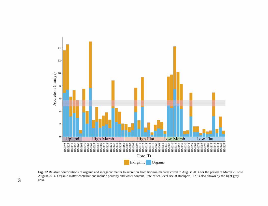
43

Fig. 22 Relative contributions of organic and inorganic matter to accretion from horizon markers cored in August 2014 for the period of March 2012 to

August 2014. Organic matter contributions include porosity and water content. Rate of sea level rise at Rockport, TX is also shown by the light grey

area.

44

Fig. 23 Relative contributions of organic and inorganic matter to accretion from horizon markers cored in July 2015 for the period of March 2012 to July

2015. Organic matter contributions include porosity and water content. Rate of sea level rise at Rockport, TX is also shown by the light grey area.

45

Fig. 24 Relative contributions of organic and inorganic matter to accretion from 137

Cs cores from previous study (Radosavljevic 2011). Organic matter

contributions includes porosity and water content. Rate of sea level rise at Rockport, TX is also shown by the light grey area.

46

Fig. 25 Relationship between vertical accretion rates and both organic and inorganic accretion rates from

combined (HM2014 and HM2015) horizon markers (annual time scale) and 137

Cs (decadal time scale). a)

organic accretion b) inorganic accretion c) organic versus inorganic d) legend for all three graphs. Note:

These graphs do not take into account porosity and water content.

47

Discussion

The success rate of horizon marker plot retrieved over time increased slightly

from 30% in August 2014 to 41% in July 2015. The increase of plot recovery was due to

improved coring equipment in July 2015. A few horizon markers were also missed during

core operations in August 2014 due to lack of visual aids. Horizon markers in Low Marsh

environments near the main tidal creek were not obtained due to the difficulty of coring

and loss of the markers. The loss of the marker can be attributed to many factors such as

wind resuspension, wave erosion, and bioturbation mixing with organic and inorganic

matter. Man-made horizon markers using brick dust have been known to have a low

recovery rate in many studies (D.R. Cahoon and Turner 1989; Knaus and Van Gent 1989;

Nolte et al. 2012).

Comparing Vertical Accretion Rates

Comparing different methods over various time scales is difficult because of the

various processes occurring simultaneously, such as subsidence (both shallow and deep),

plant processes (above and below), sea level rise, and sedimentation (Callaway et al.

1996). Annual accretion measurements using horizon markers generally highlights

accumulation events on the marsh surface, but most likely overestimates surface

elevation change because of subsurface processes occurring below the horizon marker

(D.R. Cahoon et al. 1995). Decadal accretion measurements however, highlight

accumulation of the surface processes as well as processes, such as compaction and

bioturbation that occur within the sediment column above and below the horizon marker.

Compaction within the decadal rates, calculated from dry bulk density measurements

48

throughout the column, increased at an average rate of 0.0096 per cm (Radosavljevic

2011). The largest average rate of change in compaction, 0.1216 per cm, occurs within

the top 3 cm of the marsh surface (Radosavljevic 2011), which falls within the range of

the average depth to horizon markers, 1.4 cm. Average depth to the 137

Cs marker is

approximately 7 cm. The significant difference between the decadal rates using the 137

Cs

and the annual rates derived from the horizon markers may also be attributed to other

factors. 137

Cs measurements take into account several hurricanes since 1963 that have

passed and deposited sediments to the bayside (Table 3). There have been a total of 29

hurricanes since 1963 within 200 km of Mustang Island. The highest category was H4

named Bret in 1999 that landed in Kennedy County. Storm surge associated with

hurricanes wash sediments from the Gulf shore to the bayside opening washover channels

for a period of time. Washover fans on the bayside are the sites of tidal flats and salt

marshes. The cores from the Radosavljevic (2011) study, approximately 1 m deep,

showed several washover facies throughout the column with a sharp contact to tidal flat

facies and eolian flat facies indicating that accumulation of sediments were deposited by

a hurricane.

49

Table 3 List of hurricanes, tropical storms depression since 1963 within 200 km of Mustang Island (NOAA

2014b).

Hurricane Category Name Landed on Mustang?

H4 Bret (1999) No

H3 Celia (1970), Allen (1980) Yes, Celia

H2 Beulah (1967) and Dolly (2008) No

H1

Edith (1971), Fern (1971), and

Claudette (2003)

Yes, Fern

Tropical Storms

N=14 Yes, Candy (1968) and

Charley (1998)

Tropical Depression N=7 No

Vertical accretion rates on the decadal scale are expected to be lower because of

physical compaction and decomposition of organic matter. Tidal flat rates were much

lower than all Environments regardless of Time Scale, which points to future potential

loss in this habitat zone, although the ANOVA for Low Flat environment (Fig. 14d;

Table 1) should be taken with caution because there was only one sample representing

Low Flat using 137

Cs. The most significant differences in vertical accretion between

horizon markers and 137

Cs were for High Marsh and Low Marsh environments. Previous

studies have indicated that pore space is often one of the most important factors affecting

the overall accretion rate in sandy environments because it can potentially occupy as

much as 30-40% of the sediment volume (McLachlan and Turner 1994; Callaway et al.

1996). This is especially true for short-term studies that measure surface processes.

Porosity of sediment depends on the arrangement or packing individual grains. Removing

50

pore space volume from this study significantly reduces the annual accretion rates to

within the range of decadal accretion rates (Fig. 26). Pore space was removed by only

taking into account organic and inorganic contributions calculated from bulk density

measurements as follows:

𝑃𝑜𝑟𝑒 𝑆𝑝𝑎𝑐𝑒 = 𝑉𝑒𝑟𝑡𝑖𝑐𝑎𝑙 𝐴𝑐𝑐𝑟𝑒𝑡𝑖𝑜𝑛 (𝑚𝑚 𝑦𝑟−1) − (𝑂𝑟𝑔𝑎𝑛𝑖𝑐 𝐶𝑜𝑛𝑡𝑟𝑖𝑏𝑢𝑡𝑖𝑜𝑛 (𝑚𝑚 𝑦𝑟−1)

+ 𝐼𝑛𝑜𝑟𝑔𝑎𝑛𝑖𝑐 𝐶𝑜𝑛𝑡𝑟𝑖𝑏𝑢𝑡𝑖𝑜𝑛 (𝑚𝑚 𝑦𝑟−1))

Erosion pin accretions were also significantly different to 137

Cs (p < 0.1), but not

to both HM2014 and HM2015 accretion rates (p > 0.1). Erosion pins offer a higher

frequency of measurements which usually increases the variance. The high amount of

variation in erosion pins made it difficult to observe differences to annual accretion rates

using horizon markers, but not the decadal accretion rates using 137

Cs. By measuring

accretion rates bi-weekly and annualizing we are able to capture the dynamic changes

occurring on the marsh surface throughout the year. Erosion pins take into account

accretion and erosion from episodic and spatially variable events that occurred

throughout the year, which may have reduced the overall mean for some Environments

(Fig. 16).

51

Fig. 26 Organic and inorganic contributions of HM2014 (top) and HM2015 (bottom) excluding pore and

water space.

52

Focusing on Erosion Pins

Although vertical accretion rates over the two week periods had a substantial

amount of variation over time, ANOVA results indicated significant differences in

accretion by Environment (Fig. 16). Variations in Tidal Flats containing a thick layer of

algal mat were often caused by gas filled voids producing a spongecake structure during

flooding events. Variations were also caused by eolian sediments deposited on Tidal Flats

often delivered from surrounding barren flats. The high accreting outlier in the Low Flat

environments was caused by a buildup of algae after a long period of inundation (Fig.

16). Upon returning two weeks later the accreting algae dried up and shrunk to a thin

layer of algal mat. High Flat environments overall remained fairly consistent with the

exception of one eroding site near a high traffic area. Although the erosion pin was never

disturbed by vehicle tire tracks, it was disturbed by wildlife, most likely coyotes roaming

around. Small variations in Low Marsh environments were mostly due to bioturbation.

The high accreting outlier in Low Marsh environments was due to aeolian transport

similar to a few High Marsh environments along the same area (Fig. 16). The high

accretion in August 2014 is an example of a short-episodic event that strongly influences

sediment accretion.

Comparing Short-Term Accretion Rates

Short-term monitoring over the two periods using the marker horizons did not

indicate significant differences in accretion rates between March 2012 – August 2014

(P2014) and August 2014 – July 2015 (P2015). The two different time periods show a

53

large amount of variation within each Environment making it difficult to distinguish any

differences. When observing total accretion (mm) between the two time periods however

there is a significant difference (p < 0.1) indicating that significant sediment transport

occurred in P2014 to generate slightly higher accretion. Erosion in some areas was most

likely caused by heavy rainfall during the fall and winter months of 2014. Before coring

in August 2014, the windy, arid climate caused unconsolidated, fine sand sediments to

move quickly across the marsh surface. This caused high sediment accretion in some

areas that were captured in the August 2014 cores. Caution is taken when interpreting the

difference in accretion rates between P2014 and P2015 because very few cores were

comparable (N=33).

Correlation to Elevation

The linear models used to investigate the relationship between vertical accretion

and elevation showed different correlations when grouped by environment. Linear

models were split into two groups, salt marsh only and all data, because the presence of

vegetation has been known to modify physical process by efficiently trapping more

sediment. Linear models do not include Upland environments for HM2014 and HM2015.

Vegetation could not be further reduced to species level due to lack of representative

horizon marker plots. Removing tidal flats greatly improved the model; however

removing poor quality values reduces the significance for both HM2014 and HM2015

saltmarsh only data (Fig. 17 and 18). This is most likely because very few horizon marker

plots in the low marsh environment were recovered, and those that were recovered were

questionable. Both annual scale accretion rates using horizon markers follow the same

negative correlation patterns as the decadal scale accretion rates calculated using 137

Cs, as

54

elevation decreases there is an increase in vertical accretion (Fig. 19). The rate of change

however differs between the two time scales due to differences in accretion rates in low

marsh environments. The negative correlation follows previous studies along the Gulf

coast, stating that at lower elevations there is a higher probability of sediment deposition

due to tidal influences (Pethick 1981). That assumption may not necessarily be the case

for this study area due to the strong influence of wind on the geomorphology, but the

presence of vegetation may be helping to trap sediment more efficiently whether

transported by tidal or aeolian processes.

Relative Contribution of Organic and Inorganic Matter

Sediment accumulation in wetlands consists of organic and inorganic matter,

although the ratios vary among salt marshes. Organic matter is generally considered more

important than inorganic matter for vertical accretion because it maintains the soil’s

stability, water volume, and sustains pore space (Turner et al. 2002). The relative

contributions on a dry weight basis indicate that inorganic matter overwhelmingly

dominates accretion on Mustang Island; however, this contribution is less evident after

associating pore space and water content to organic matter (Fig. 22, 23, 24). Previous

studies have attributed pore space volume to organic matter because of its strong

correlation with water (Bricker-Urso et al. 1989). Following this assumption, the ratio of

organic to inorganic matter contribution for vertical accretion is approximately 1:1,

although there is some skepticism using this theory due to differences in climate.

The importance of inorganic contribution is evident by the significantly linear

relationship between accretion and inorganic accretion (Fig. 25b). Vertical accretion rates

55

for this area are directly related to both organic and inorganic matter, although the

relationship with inorganic matter has a stronger correlation (r2 = 0.91). On average

Upland environments had the least percent of organic matter content (1.54 ± 0.7 %),

while Low Algal Flat had the greatest organic matter content (6.44 ± 3.4 %). The linear

trend of increasing percent organic matter from Upland to Low Algal Flat is shown in

Fig. 21. The organic and inorganic accretion rates also show this linear trend in

increasing organic matter from Upland to Low Marsh environments indicating that

organic matter contributions are more significant in Low Marsh environments than

Upland (Fig. 25c). Overall organic and inorganic accretion rates for horizon markers

follow the same patterns as 137

Cs, dominated by inorganic matter (Fig. 25a, b). The strong

correlation with inorganic matter in short-term and longer-term studies suggests that

Mustang Island vertical accretion rates are influenced by the amount of inorganic matter

deposited in the area. The dominance of inorganic matter helps reinstate the fact that the

area depends greatly on episodic inputs from storms to maintain its elevation, which often

brings inorganic matter.

56

Fig. 27 Comparison of the relationship of vertical accretion with organic and inorganic accretion in the

present (MUI Horizon Marker) and previous study (MUI 137

Cs) for this area as well as other localities a)

organic accretion, b) inorganic accretion, c) organic versus inorganic accretion, d) legend for all plots

indicating locations. Data of other studies are from Turner et al. (2002) for Upper Texas coast, Louisiana,

and Rhode Island, and data for Texas (Aransas National Wildlife Refuge), San Bernard, Mississippi, and

Florida Keys are from Callaway et al. (1997).

57

When comparing organic and inorganic accretion rates in marshes of other

geographic areas, organic matter accretion for this study area appears to contribute much

less to vertical accretion (Fig. 27). The dominance of inorganic matter is due to the

generally drier and wind dominated character of wetland environments on Mustang

Island in comparison to other geographic areas. Lower, frequently inundated

environments in Mustang Island are more similar to marshes in Rhode Island, Florida and

Mississippi (Fig. 25 and 27). Previous studies have shown that there is an upper limit to

the amount of organic accretion, causing marshes to be lost to rising sea levels despite

having high accretion rates (McCaffrey and Thompson 1980; Bricker-Urso et al. 1989;

Turner et al. 2002). Results from this study follow similar patterns to marshes in

Louisiana receiving high amounts of inorganic sediment, and very little organic matter.

Both studies appear to reach an asymptote in the relationship between organic versus

inorganic, which suggests that organic accretion cannot match such high rates of

inorganic accretion (Fig. 28). Inorganic sediment has been shown to play an important

role creating a positive feedback loop with plant growth by increasing particulate

nutrient, which is shown by the positive relationship between organic and inorganic

matter (Fig. 25 b, c). It is important to keep in mind that the studies shown in Fig. 27, all

used radiometric dating methods using the 137

Cs marker (decadal accretion rates)

therefore the vertical accretion rate in this study using horizon markers (annual accretion

rates) are expected to be higher.

58

Fig. 28 A comparison of the relationship between organic accretion and inorganic accretion. a) This study combined with Radosavljevic (2011), b) Louisiana

studies from Fig. 20. Shaded regions indicate 95% confidence interval. This figure is the similar to Fig. 20c except the geographic localities are plotted separately

for visualization.

59

Grain Size

Grain sizes are often used as a means of distinguishing coastal environments of

deposition (Simms et al. 2006). Grain size distribution did not differ very much between

HM2014 and HM2015 with the exception of additional measurements in HM2015 due to

increase in plot recovery. The majority of the horizon marker plots were classified as fine

sand, and a few algal flats classified as silty sand. Upland environments were 100% sand,

while High Marsh, High Flat, and Low Marsh environments had slight variations, but

remained classified as fine sand. Grain sizes became finer going from Upland to Low

Algal Flat environments (Fig. 20). Differentiating sediment grain size using means is

difficult for Mustang Island due to the uniformity of fine grain sizes across the marsh.

Implications for Sea-Level Rise and Marsh Loss

The rate of relative sea-level rise (RSLR) for this area over the last ~77 years

(1937 – 2014) has been 5.27 mm yr-1

, as recorded by the Rockport, TX tidal gauge

station (NOAA 2014a). Accretion rates using horizon markers appear to be “keeping up”

with RSLR in Low Marsh (~11-12 mm yr-1

) and Upland environments (~7-8 mm yr-1

),

but not Tidal Flats or High Marsh environments that sit just above Low Marsh

environments in elevation. The range in elevation of the Mustang Island environments is

minimal ranging from ~0.2 m to ~0.7 m, therefore even a small increase in tidal range

can greatly influence this area (Fig. 29).

60

Fig. 29 Range of elevations for each environment. Low flat elevations vary in this area, but are generally

considered to be at lower elevations than low marsh environments.

Tidal flats, which are important avian feeding habitats, will more than likely be

converted to low marsh environments, while the low marsh environments will likely

convert to open water. The short-term accretion rates categorized by environment follow

the same patterns as the decadal rates from 137

Cs (Fig. 13), but are significantly higher

due to pore space. Decadal accretion rates across all environments do not appear to keep

pace with RSLR for this area. Consequentially, changes in environmental states are

expected to occur as sea-level rises as we have seen in the past (Fig. 30). The rate of

change is what differs between the two time scales. There is a greater deficit for accretion

rates in Low Flat (~1.5-2 mm yr-1

) environments relative to sea-level rise rate (~5 mm yr-

1), which may explain the findings of (White et al. 2006) shown in Fig. 30. Tidal Flat loss

for Mustang Island has been declining since the 1950s, showing a transition of

environmental states from Tidal Flat to Low Marsh due to absence of washover channels,

Upland High Marsh High Flat Low Marsh Low Flat

0.2

0.3

0.4

0.5

0.6

0.7

Ele

vat

ion

(m

, N

AV

D8

8)

61

and fewer connections to estuarine systems (White et al. 2006). This has caused upland

vegetation to stabilize dunes along the west side of Mustang Island.

Fig. 30 Map showing wetland transitions from 1950’s, 1979, and 2002-04 for Mustang Island and Harbor

Island (White et al. 2006). Study area in Mustang Island is highlighted by the red box.

Estuarine marsh

Flats/beaches

Palustrine marsh

Aquatic beds

Scrub/shrub

Upland

0 5 102.5Km

2002-04 1979 1950's

1950 1979 2002-04

62

Conclusion

Vertical accretion rates were significantly different between annual scale and

decadal scale measurements. Decadal vertical accretion rates are much lower because of

the different processes being measured, as well as compaction and decomposition

throughout the core. Sediment accumulation for the period of 2014 to 2015 was minimal,

although there was high variation in accretion/erosion throughout the study as indicated

by the erosion pins. Inorganic matter was the major contributor for vertical accretion in

Mustang Island, which is drastically different than other geographic areas. This is due to

the arid, wind-dominated climate associated with Mustang Island. According to short-

term accretion rates Low Marsh environments are capable of keeping pace with RLSR;

however the area is expected to undergo changes in environmental states due to the low

amounts of organic matter contributing to vertical accretion. Mustang Island depends

greatly on episodic inputs from storms to maintain its elevation. Although hurricanes

often generate impacts detrimental to the environment, they also have potential benefits

by supplying large areas of coastal marsh with sediment. When storm-induced sediment

is sufficient, stability of coastal marshes may be enhanced for some time to help cope

with RSLR (Baustian and Mendelssohn 2015).

63

Chapter 3: Assessing Hydrological Influences

Introduction

In many estuarine wetlands throughout the Gulf of Mexico, hydroperiod, which

consists of flooding frequency and duration, is considered one of the major factors

controlling sediment deposition (D. R. Cahoon and Reed 1995).Winds, precipitation,

evaporation, astronomical tides, and fluctuating regional sea levels influence water levels

occurring in wetlands throughout the year. Marshes that are remote from a riverine source

such as Mustang Island rely on winter storms, tropical cyclones, and strong winds for

mobilizing sediments into the marsh. During storms, water levels are raised high enough

to flood the marsh and potentially deposit sediment. Tidal creeks are the system through

which sediments, organic matter, nutrients, and pollutants are transported into and out of

the wetlands. Sediment sources for remote marshes are largely related to resuspension of

existing sediments adjacent to the marsh environment. Hurricanes, on the other hand,

have the ability to transport large pulses of sediment onto the marsh surface through

washover channels. The sediment sources from hurricanes can come from bay and ocean-

side dunes and beaches washed over during the event. The major hydrodynamic

characteristics proposed by Gosselink and Turner (1978) are the water inputs, water

outputs, type of water flow, and hydropulses (seasonality).

Previous studies have illustrated the importance of microtopography in

controlling flooding regimes (Reed and Cahoon 1992). Variations within 0.04 m across

the marsh surface are able to produce significant changes in hydroperiod (Swenson and

Turner 1987). Variation in topography causes areas of the marsh to be flooded more

frequently and for longer periods than others. Evapotranspiration and tidal flooding can

64

also affect soil volume and precise marsh surface levels (Paquette et al. 2004). Surface

and groundwater circulation rate are also vital to the sedimentation process, chemistry,

and biological processes due to the strong feedback loop between circulation, sediment

dynamics, and the constantly changing geomorphology (Perillo et al. 2009). Vegetation

often provides important clues of hydrogeomorphic forces in an ecosystem (Brinson

1993). Sources of freshwater in salt marshes can come from river input, groundwater

flows, or as a result of rainfall. The overall freshwater input for Mustang Island is

determined by meteorological conditions, such as the precipitation and evaporation

balance. There are two effects of rainfall on salt marshes, reduction in soil salinity and

the flow of water across the surface of the marsh with the potential for eroding,

transporting, and depositing sediment within the wetland. In this study we examined the

relationship between wetland topography, hydroperiod, and sediment accumulation over

a period of 12-months. Results from this study will further our understanding of sediment

delivery into the marsh system through tidal processes thus having important implications

for wetland development and management. This study aims to answer the following

questions:

1) What is the relationship between hydroperiod and sediment accretion?

2) How much organic and inorganic matter is associated with hydroperiod?

This information will contribute to our understanding of the hydrological influence to the

sediment accretion of a brackish salt marsh.

Materials and Methods

Water Level Loggers

65

Eighteen water level loggers (WLL) were used to measure water depth and

temperature (Fig. 31). Data were acquired at defined intervals and stored in each WLL

until it was downloaded in the field. The WLL use pressure transducers to measure water

depth, therefore, data need to be adjusted for atmospheric pressure.

Fig. 31 Distribution of water levels loggers on Mustang Island, TX.

There were two types of water level loggers used in this study:

Water Level with a vented cable, which is capable of correcting for atmospheric pressure

automatically (OTT Orpheus Mini)

Water level non-vented with no cable (completely submerged), which needs corrections

for barometric pressure. Barometric pressure was acquired from the Packery Channel

tidal gauge less than 10 km from the study area and operated by the Texas Coastal Ocean

Observation Network at TAMU-CC.

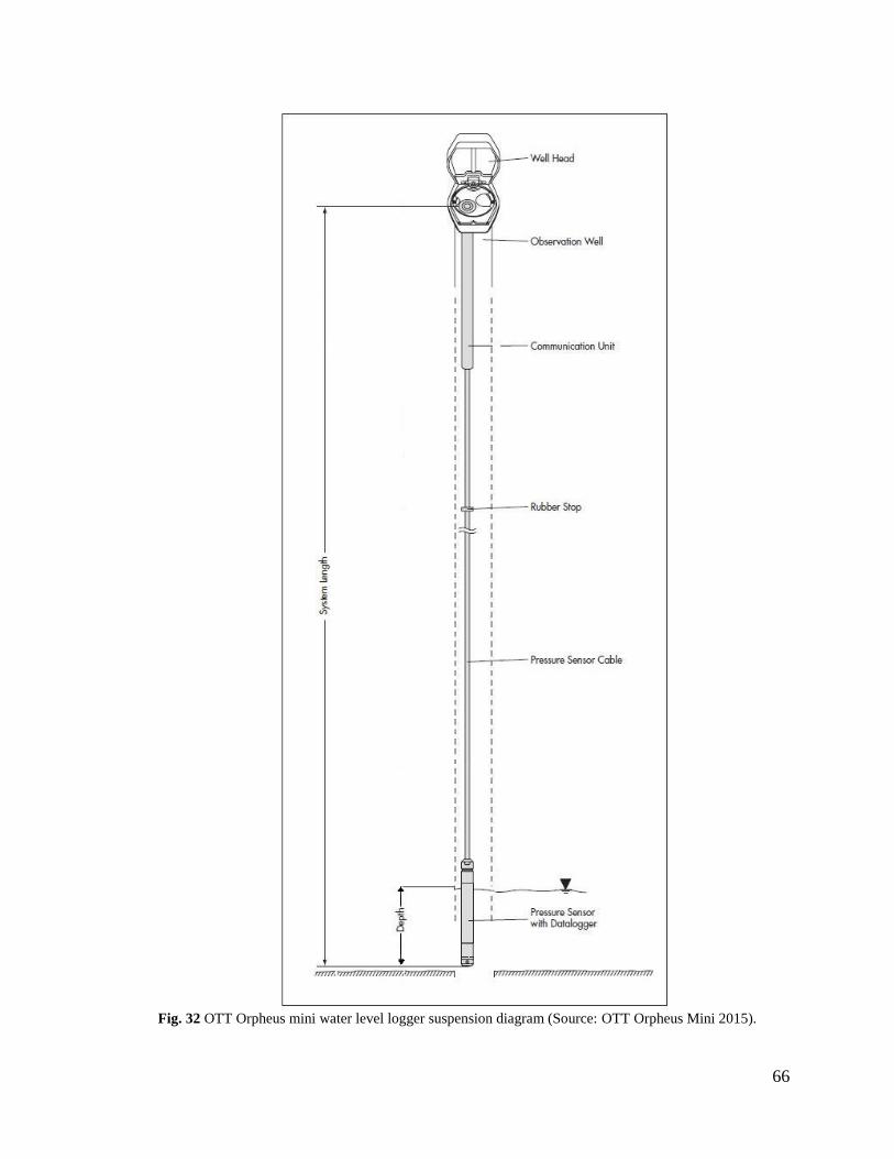
66

Fig. 32 OTT Orpheus mini water level logger suspension diagram (Source: OTT Orpheus Mini 2015).

67

Fig. 33 HOBO Onset water level logger deployment diagram (Source: HOBO Onset 2015).

Technical Information

The OTT Orpheus Mini is 1m in length with a water level measuring range from 0 –

4 m with an accuracy of ± 0.05% full scale (FS) or ±0.2 cm (Fig. 32). The temperature

measuring range is from -25˚C to +70˚C with an accuracy of ± 0.5˚C. Measurement

memory for data is 4MB (approximately 500,000 measurements). The HOBO Onset

U20L-04 is about 15 cm in length with water level measuring range from 0 – 4 m and

accuracy of ± 0.1% FS or ± 0.4 cm (Fig. 33). The temperature range is from -20˚C to

50˚C with an accuracy of ± 0.44˚C. Measurement memory is 64KB (approximately

21,700 measurements).

Deploying Device

Criteria used to define location of water data loggers:

Must be within 1 m of a retrieved marker horizon

Preference is for clustered markers

Must have at least one logger in each geoenvironment type (High Marsh, Low

Marsh, and Tidal Flats)

A logger must be in each of two major tidal creeks (HOBOs were used for these

sites)

68

Orpheus Mini water level loggers were deployed using a 2.5 m fence post and 2.5 cm

diameter Schedule 40 PVC pipe 1 m in length (Fig. 32). The fence post was driven into

the ground leaving 1 m exposed to attach the PVC pipe with two steel hose clamps. The

Orpheus Mini is suspended in the protected well using a 2.5 cm adapter ring (Fig. 32).

Immediately after installing the OTT Orpheus Mini, the sampling interval was set to

record water level and temperature every six minutes using the OTT Water Logger

Operating Program. The time of every action, such as placing the batteries, deploying the

logger in the water or adjusting it to the appropriate level was recorded throughout the

study. Batteries were easily replaced by removing the pipe encasing the communication

unit located at the top. Water depth and time was recorded each visit to ensure accuracy

of the data. Sensors were placed ~1 cm above ground level to prevent sediment build-up

potentially blocking sensors.

Two HOBO water level loggers were deployed using cinder blocks as a method for

attachment (Fig. 33). The water level logger was also housed in a PVC pipe for

biofouling protection and was attached to the cinder block using zip-ties. HOBOs were

deployed in the main tidal creeks (WLL16 and 17) because the Orpheus Minis were not

capable of being completely submerged. HOBOs were attached to PVC wells using thin

nylon rope. One HOBO (WLL18) was used in a high marsh environment. An extra

HOBO was reserved as a backup.

Surveying Loggers

The elevation of the water level logger was measured using a RTK GPS at the top of

the logger as well as the base, so that water depth data can be converted from relative

depth to elevation or a tidal datum to allow for comparison among sites. Horizontal

69

coordinates were set to NAD83, vertical coordinates were set to NAVD88 using the

hybrid geoid model GEOID09. RTK GPS uses Virtual Reference Stations (VRS) as base

stations in order to reduce initialization time. The use of a network of reference stations

instead of a single reference station allows to model the systematic errors in the region,

which reduces the possibility of error (Landau et al. 2002). The VRS network stations are

continuously connected to a control center, gathering information from all receivers.

Initially the GPS rover needs a minimum of three reference stations that are connected to

the network server. Using VRS GPS, the rover sends its position to the control center

using a mobile phone data link. The control center then accepts the position and responds

by sending RTCM correction data to the rover to compute a high quality DGPS position

solution, and update its position. The network server calculates new RTCM corrections,

so that they appear to come from a station right beside the rover to give DGPS solutions

accurate to within 2 cm in the horizontal plane and 4 cm in the vertical direction (Landau

et al. 2002; Petovello 2011). During measurements and maintenance, it is critical that the

logger remain in the same location otherwise the elevation of the logger must be surveyed

each time the logger is moved.

Programming Data Logger

Data logger settings were set directly by connecting the device to a computer using an

IrDA – Link adapter (OTT) and a Coupler (HOBO). For each site, the measurement

station number and name was adjusted in the operating program to have a unique

identification for referencing. Time was adjusted to match the computer for consistency

in Universal Time Coordinate (UTC). After water level loggers were installed, water

level values were instantly viewed on the computer software program and corrected

70

respectively. Sampling interval for this study was adjusted to six minutes to match the

Texas Coastal Ocean Observation Network (TCOON) tidal gauge measurements for

reference.

Maintenance Work

The pressure probes were cleaned every other week to prevent accumulation of

barnacles, and heavy contamination due to algae, mud or sediment. Data was always

collected before cleaning the pressure probe. The pressure probe was cleaned easily by

removing the black protective cap from the sensor (OTT). Sensors were cleaned carefully

using a small brush (OTT) or using a cotton swap (HOBO). After probes were cleaned

they were placed carefully back into the well.

Assessing Hydroperiod

Start and end times of duration and depth of the flooding event for each sediment

plate was determined from survey data. Survey data was used to calculate the difference

in elevations between the sediment plate and the nearest water level logger to determine

water level estimates at the sediment plate (Fig. 34). The hydroperiod data was summed

for each sampling interval in order to establish the flooding regime during the sampling

period. From survey data, flood duration events, flood duration events with time and

depth, max water level, and number of flooding events were calculated. Duration (min)

was calculated using the summation of minutes that the sediment plate was flooded.

Duration in time and depth was calculated using the minutes the plate was flooded

multiplied by the depth (water column) during each six-minute interval. Number of

flooding events is simply the total count the sediment plate was exposed based on

71

elevation and water level as explained by Fig. 35. Distance to tidal creek from each

sediment plate was determined using a least cost path analysis in ArcMap 10.2. Least cost

path tool utilized a digital elevation model to create a slope and cost back-link raster.

Fig. 34 Schematic of hydroperiod measurements at sediment plates using nearest water level logger.

Fig. 35 Example of how number of flooding events were counted. F1 indicates 1

st count of flooding event,

and continues to F4, so in this example Number of Flooding Events = 4 (number of time sediment plate

was exposed after initial flooding event).

Sediment Plate Flooded

Wat

er L

evel

(m

)

Time

F1 F2 F3 F4

72

Sediment Plates

For each water level logger in this study, there was a corresponding set of sediment

plates, with the exception of all HOBOs. The sediment plates were made of plexiglass 7.5

cm in diameter and 3 mm thick similar to plates used by Kleiss (1993) (Fig. 36). A hole

1.5 cm in diameter was made in the center to attach a threaded PVC rod and threaded

nylon washer to secure the plate. There were 30 sediment plates installed: 11 in high

marsh (HM); 9 in low marsh (LM); and 10 in high and low tidal flat (TF) environments

(Fig. 37). They were left to accumulate sediment approximately every 2 weeks from July

2014 to July 2015. RTK GPS measurements were taken recording x, y, z coordinates for

each sediment plate. Sediment plate sites were chosen following the criteria below:

Criteria for sediment plate locations for this study:

Must be within 1 m of the marker horizons

Preference given to grouped markers

Fig. 36 Circular sediment plate modeled after Kleiss (1993). Diagram of sediment plate (left), sediment

plate example from low marsh environment after flooding event (right).

73

Fig. 37 Sediment plate distribution on Mustang Island, TX.

Sediment plates were revisited approximately every two weeks depending on an

event of heavy precipitation. When revisiting, sediment traps were removed to carefully

collect the accumulated sediment on top and placed in a sealed jar. Sediment adhering to

the bottom of the plate was removed in the field. Removed sediment plates were replaced

by clean ones each time. Sediment plates were left in place if they were flooded more

than 2 cm at the time of collection. In the lab sediment samples from the plates were

placed in pre-weighed jars washed with distilled water. Samples were then dried at 60˚C

for 24 hours or more if needed and weighed to calculate mass sedimentation rates,

expressed as g cm-2

. Sediment deposition was calculated by dividing the number of grams

by the surface area of the circular plate (minus the surface area of the threaded rod).

74

Samples with sufficient sediment were split to analyze grain size, and organic/inorganic

matter.

Sediment Characterization

Organic Matter Content

Organic matter methods were similar to Chapter 2.

Grain Size

Sediment grain size methods were similar to Chapter 2.

Results

A few months after water level loggers were deployed in July 2014 a few water

level loggers began to lose function over time. By the end of the study, two water level

loggers remained accurate (WLL4 and WLL8) and one (WLL9) was replaced with an

extra HOBO water level logger (Fig. 31). WLL14 and WLL15 were not included in any

data analysis. WLL data only includes accurate water level logger data up to the point of

water level logger failure for analysis. Because of this loss, there were several sediment

plates that were collected, but did not have hydroperiod data thus reducing data.

Hydroperiod

Influence on Sediment Deposition

Initial data exploration was performed using a pairs plot to observe relationships

among all factors, which include duration of flooding (min), duration in time and depth

(min*m), max water level, number of flooding events, and distance to tidal creek. The

relationships between sediment deposition and hydroperiod variables were tested by

multiple regression analysis. Variable inflation factors were computed to determine if

there was significant collinearity among the predictor variables. Based on this

75

information, as well as an exhaustive search of all linear models, a preliminary model

was made using the following criteria:

1. Small Akaike’s Information Criterion correction (AICc) values, based on

maximum likelihood fittings

2. Significance level of α = 0.1 for any variable included

3. And diagnostics at least as good as comparable models

The diagnostic tests, which include normality, heteroscedasticity, and Cook’s distance, of

the final model were checked to ensure that any model inference was valid.

Before plotting data observations, all sediment plates that accreted from

bioturbation (N=35) were removed from data analysis to prevent skewed results.

Accretion caused by bioturbation from fiddler crabs was common throughout the study.

An initial scatterplot of the deposition on the sediment plates for each sampling period

and location (N= 293) showed no significant correlation with duration (p > 0.1, Fig. 38a).

Sediment plates that were estimated to be flooded however did show a slight correlation

(Fig. 38b). Relationships between deposition and duration for both scenarios (all

sediment plates and only flooded sediment plates) show a slight positive correlation when

converting the y-axis to log-scale, although there is a substantial amount of variation of

deposition for durations near zero (Fig. 38 c, d). A few algal flat environments had the

longest duration, but very little accretion, while some algal flat environments were hardly

flooded. Lower plots flooded more frequently than higher plots as shown by the

significant negative correlation between Frequency and Elevation (p < 0.1; r2= 0.18),

although a substantial amount of variation is left unexplained. The variation in marsh

topography combined with wind processes had a clear effect on sediment deposition.

76

It is expected that sites with a longer hydroperiod would have increased

deposition; therefore, a separate scatterplot was created to only include sediment plates

that lie along the main tidal creek (N= 50). Plates included: LM1, LM2, LM4, LM8,

LM10 (Fig. 37). Sediment deposition for plates near the main tidal creek had a

significantly positive correlation with number of flooding events and duration in time and

depth (Fig. 39). Using plates closer to the tidal creek significantly improved the

correlation with duration and flooding events (p < 0.1); although diagnostics plots

indicated there were some slight problems with heteroscedasticity caused by two

influential points (Fig. 39).

77

Fig. 38 Relationship of sediment plate deposition with flooding duration in time and depth. a) all sediment plates, b) only sediment plates

that were flooded, c) all sediment plates with y-axis log scaled, d) only flooded sediment plates with y-axis log-scaled.

78

Fig. 39 Relationship of sediment plate deposition with number of flooding events (a) and duration in time and depth (b) for plates in low marsh environments

near the main tidal creek only.

79

Several linear models were evaluated and further reduced to the equation in Fig.

39a which includes Number of Flooding Events as the fixed factor. The linear equation

including Number of Flooding Evens was chosen as the best model based on the criteria

preciously stated. Although a separate model, which included both Number of Flooding

Events and Duration in Time and Depth as fixed factors, explained a higher percent of the

variability in deposition, it was eliminated because the Duration in Time and Depth factor

was not significant after adjusting for heteroscedasticity (p > 0.1). Using Number of

Flooding Events, 50% of the variation in sediment deposition can be explained

significantly (p <0.1). The r2 value decreased slightly from 62% to 52% for linear

equation in Fig. 39a after fixing heteroscedasticity.

Organic and Inorganic Matter Associated with Hydroperiod

Relative contributions of organic and inorganic matter were calculated from the

weight of the sediment accumulation and results from LOI methods as follows:

𝑂𝑟𝑔𝑎𝑛𝑖𝑐 𝐴𝑐𝑐𝑢𝑚𝑢𝑙𝑎𝑡𝑖𝑜𝑛 (𝑔 𝑐𝑚−2) = 𝐿𝑂𝐼/100 (%) ∗ 𝑆𝑒𝑑𝑖𝑚𝑒𝑛𝑡 𝐷𝑒𝑝𝑜𝑠𝑖𝑡𝑖𝑜𝑛 (𝑔 𝑐𝑚−2)

𝐼𝑛𝑜𝑟𝑔𝑎𝑛𝑖𝑐 𝐴𝑐𝑐𝑢𝑚𝑢𝑙𝑎𝑡𝑖𝑜𝑛 (𝑔 𝑐𝑚−2)= 𝑆𝑒𝑑𝑖𝑚𝑒𝑛𝑡 𝐷𝑒𝑝𝑜𝑠𝑖𝑡𝑖𝑜𝑛 (𝑔 𝑐𝑚−2) − 𝑂𝑟𝑔𝑎𝑛𝑖𝑐 𝐴𝑐𝑐𝑢𝑚𝑢𝑙𝑎𝑡𝑖𝑜𝑛 (𝑔 𝑐𝑚−2)

Hydroperiod exerted a positive influence on organic and inorganic accumulation

processes for sediment plates (N=16) near the main tidal creek (Fig. 40). Organic and

inorganic matter contributions were both significantly correlated with the duration of the

plates (p < 0.1). Duration in Time and Depth of flooding explained 64% and 79% of

variation in accumulation of inorganic and organic matter respectively. Once again

diagnostic tests indicated very slight problems with heteroscedasticity caused by the two

influential points. This was only a slight problem for the linear model including inorganic

accumulation. There were no diagnostic problems for the linear model including organic

80

matter accumulation. Heteroscedasticity was not drastic enough to use variance functions

to correct problems. Plates closest to the main tidal creek (LM4 and LM8) had the highest

accumulation for both organic (~0.12 g cm-2

) and inorganic matter (~ 1.5 g cm-2

) (Fig.

40). Accumulation of matter does not take into account sediment porosity, density, or

water content.

Fig. 40 Relationship between accumulation of both organic and inorganic matter with duration in time and

depth. Accumulation of matter does not take into account sediment porosity, density or water content.

Water Levels

Water level calculations were estimates of how much water should be on the

marsh surface. The data does not take into account ponding effects that could possibly

increase duration and frequency for sediment plates. Water level patterns were highly

dependent on local proximity to tidal creeks and heavy rainfall. Duration of total flooding

81

events considering all sites (N= 293) ranged from 102 minutes in a high marsh

environment with sparse short grass to 336,732 minutes (~233 days) in a low tidal flat

environment with no vegetation covered by a thick layer of algal mat. These longer

flooding events were related to prolonged stagnant high-water across tidal flat

environments during September caused by high tides coupled with heavy local rainfall

throughout the winter and spring. The deepest flooding event for plates along the main

tidal creek occurred during September 28, 2014 (Fig. 41). LM2 was the deepest plate

flooded with a maximum water level of 43 cm (Fig. 41). Water level readings near the

main tidal creek indicate a seasonal hydroperiod pattern throughout the study with the

most flooding events occurring during Fall/Winter and Late Spring (Fig. 41).

Fig. 41 Water level referenced to NAVD88 near main tidal creek, including sediment plate elevations.

Horizontal lines represent elevation of sediment plates on the marsh surface.

82

Grain Size Analysis

To explore potential influences on sediment deposition, grain size analysis of

sediment samples was conducted. Only sediment samples with sufficient sediment for

both grain size and organic matter were split for analysis. If sediment samples from plates

did not have sufficient sediment they were combined with other sediment samples from

the same plate location. Grain sizes from sediment plate samples with no bioturbation

(N=49) throughout the year were analyzed (Fig. 42). Lower elevations (0.1 m -0.3 m)

were mostly silty-sand and sandy-silt according to the Shepard classification (Fig. 42b).

These areas are also classified as algal mats, and low marsh environments (Fig. 42a).

Grain sizes from sediment plates with no bioturbation near the main tidal creek (N=

15) were plotted separately for further observations (Fig. 43). Plates closest to the main

tidal creek (LM4 and LM8) had a grain size range from sand to silty sand (Fig. 43a).

These plates consisted of Avicennia germinans and Spartina alterniflora vegetation (Fig.

43b). LM1 and LM10 plates are at a slightly higher elevation relative to LM4 and LM8

(Fig. 41) and were classified as sand with vegetation cover consisting of succulents and

mangroves. Although LM2 has the lowest elevation it is also the farthest from the main

tidal creek (Fig. 37).

83

Fig. 42 Sediment grain size for all sediment plates, excludes plates with bioturbation. a) grain size classified by vegetation type, b) grain size classified by range

of elevation.

84

Fig. 43 Sediment grain size for plates near the main tidal creek, excludes plates with bioturbation. a) grain size classified by sediment plate ID, b) grain size

classified by vegetation type.

85

Discussion

Bioturbation was the main process for several sediment plates, but there is

skepticism by some whether this qualifies as true deposition or redistribution of sediment

already on the marsh surface. For the purpose of this study, sediment plates that accreted

due to bioturbation were omitted from analysis of results. Bioturbation was detectable by

the presence of small pellets formed from fiddler crabs.

There are several factors that influence sediment deposition, as shown by the lack

of correlation between deposition and duration and time and depth and high variation

near zero in Fig. 38. The highest deposition of 37.8 g cm-2

occurred in a low marsh

environment near a dry tidal creek. This occurred in late August 2014, accreting about

10.2 cm in a period of approximately two weeks. Two other plates (LM9 and HM9) also

along the northwest side of the salt marsh also accumulated high amounts of sediment

(7.3 and 6.68 g cm-2

, respectively) in an earlier period during late-July 2014. The

accretion for LM9 was 3.95 cm, and the accretion for HM9 was 2.45 cm over a period of

two weeks. Strong southeasterly winds were the main process driving sediment accretion

for these episodic events (Fig. 38a). Aeolian suspended sediment accumulation varied

widely over short time periods and distances across the marsh surface. At the other end of

the spectrum, there were plates that were flooded throughout most of the study (TF5 and

TF6), but accreted very little sediment. Accretion for these sediment plates occurred from

the stagnant water that lingered throughout the year eventually creating a new layer of

algal mat, about 4mm thick. The low r2 value for sediment deposition versus duration in

time and depth using all sediment plates (N=293) indicates that factors in addition to

hydroperiod had a strong influence on deposition throughout the study (Fig. 38a).

86

Previous studies for marshes on the U.S. east coast suggests that the hydrological

patterns influence the microtopography of the marsh surface through a combination of

sedimentation and erosion in a feedback with hydrological patterns that create the

microtopography on a fine scale (Frey et al. 1985). Storms however, can influence the

microtopography on a larger scale. Sedimentation deposition has been known to be

closely related to major washover events from storms for this area. Sediment deposition

through aeolian processes is also a major factor for this area due to the arid, wind-

dominated climate associated with Mustang Island, TX. Hence the results focused on

sediment plates near the main tidal creek. Results did not include tidal plates near the

most northern tidal creek because culverts near a road further restricted tidal influences

for the area. Seasonal deposition patterns could not be observed using all sediment plates

because the sampling period of some plates, such as TF5 and TF6, carried across multiple

seasons due to prolonged flooding.

Influence of Hydroperiod on Deposition

The longest flooding event for plates near the main tidal creek was 77,970

minutes (54 days) occurring from May – June 2015. The maximum depth during this

period was 42 cm for LM4 and LM8 sediment plates. The high water was caused by an

extended period of heavy rainfall in both months (Fig. 44). Tropical Storm Bill (June 16,

2015) may have influenced prolonged inundation for the area. Total rainfall throughout

the study was above average caused by the effects of a moderate El Nino, which is

expected to continue through fall 2015 and gradually weaken by spring 2016 (NOAA

2015). The total rainfall for the 2015 water year which began on October 1, 2014 was

113.51 cm which is 41.19 cm above average (NOAA 2015).

87

Fig. 44 Precipitation and wind direction and magnitude throughout the study period. Y-axis represents precipitation in centimeters. Stick plot shows

wind direction and magnitude (scaled relatively to each other). Winds pointing north (90˚) indicate winds are coming from the south headed north

88

Accumulation of sediment was strongly correlated with both flooding duration

and number of flooding events (Fig. 39). However, the relationship explains less than

40% and 62% of the variation in sediment deposition, respectively, because not all

inundations contribute the same amount of sediment. The correlation between deposition

and flooding duration is slightly influenced by the LM4 and LM8 plates, located on the

far right in Fig. 39, which were flooded during the period of May and June 2015. It may

be that the few large events, such as Tropical Storm Bill, during the May/June sampling

period accounted for most of sediment deposited on top of these plates (Fig. 44). This

was also the same time period when two cement blocks were swept away, one of which

was anchoring WLL16. The absence of the heavy cement blocks (~35lbs) helps to

visualize the strength of the currents from Tropical Storm Bill within the tidal creek that

may have attributed to such high deposition. Storms are a major influence on sediment

delivery, distribution, and deposition within Mustang Island because of the absence of a

riverine source.

Contribution of Organic and Inorganic Matter Associated with Hydroperiod

When focusing on organic and inorganic accumulation both have a strong positive

correlation with duration although inorganic matter has a larger contribution. Comparing

accumulation rates of both organic and inorganic matter in marshes of this study and of a

study in Louisiana (D. R. Cahoon and Reed 1995), results indicate that organic matter

accumulation eventually reaches a limit, and is dominated by inorganic matter (Fig. 45).

The relationship implies that organic matter was delivered to the marsh surface during

flooding events. Overall results support observations in other research that sedimentation

89

can be episodic, and that sediment delivery is not consistent for each marsh surface

inundation (Wood and Hine 2007).

Fig. 45 A comparison of the relationship between accumulation of both organic and inorganic matter and

duration of flooding (log10 scaled x-axis) in the present study, using sediment plates near the main tidal

creek, and in a study in Louisiana.

The most important factor in determining sediment deposition on sediment plates

located near the main tidal creek was the number of flooding events, suggesting that

deposition increases as frequency of flooding events increases. Thus an increase in

frequency of flooding events allows suspended sediments within the water column to

potentially be deposited on the marsh surface. The interpretation of the model should be

taken cautiously for several reasons. There were two major influential points (LM4 and

LM8) that caused the linear model to have problems with heteroscedasticity. Before

fixing problems, duration (count) and duration (integral) were highly significant,

explaining a large portion of the variation of deposition. The final model, however, gives

the best estimate available and can be used to predict the expected deposition results for

0.0

0.5

1.0

1.5

2.0

2.5

100 1000 10000Duration (hrs)

Acc

um

ula

tio

n o

f M

atte

r (g

/cm

sq)

Louisiana Study (Cahoon & Reed, 1995)

This StudyInorganic Matter Organic Matter

90

areas near the main tidal creek. The model does not work in areas further from the tidal

creek because of the dynamic environment strongly influenced by wind processes.

Grain Size

Sediments along the backside of Mustang Island are transported by aeolian,

overwash, inlet migration, or tidal process. Previous studies have attempted to

differentiate wetland environments on Mustang Island with sediment grain size

characteristics, but this has proven to be difficult because of the uniformity of sediments

in the area (Simms et al. 2006; Radosavljevic 2011). The present study used the sediment

that was deposited onto the plate for grain size analysis as opposed to previous studies

that used samples from the top 5cm.

Simms et al. (2006) and Radosavljevic (2011) were able to effectively differentiate

beach and dune sediments from barrier flat environments by observing the relationship

between skewness and mean grain size (Fig. 46). Skewness is a measure of the amount of

asymmetry in a grain size distribution compared to a normal distribution. A skewness

value of 0.2 has been determined as a threshold to differentiate between sediments

deposited by wind and finer skewed barrier flat environments. Results from this study are

very similar to previous studies (Fig. 46 and 47). Sediment grain size using all sediment

plates (N=293) suggests algal flat, and a few low marsh environments have finer sand,

classified as silty sand, and sandy silt, which contributes to the asymmetry in skewness.

Algal mat and low marsh environments are known to be much more effective at trapping

fine sediment (Frantz et al. 2015), which helps explain the gap around the skewness

threshold of 0.2 for algal flat and low marsh environments and other environments (Fig.

47). The relationship between skewness and mean grain size indicates most low marsh

91

sediments fall above the 0.2 threshold suggesting that sediments are deposited by tidal

processes. Plates at higher elevations, such as high marsh and high tidal flats also show a

trend of more symmetrical grain size distributions, thus majority lie below the 0.2

skewness thresholds (Fig. 47). This could possibly be due to the aeolian processes driving

sediment transport to those areas.

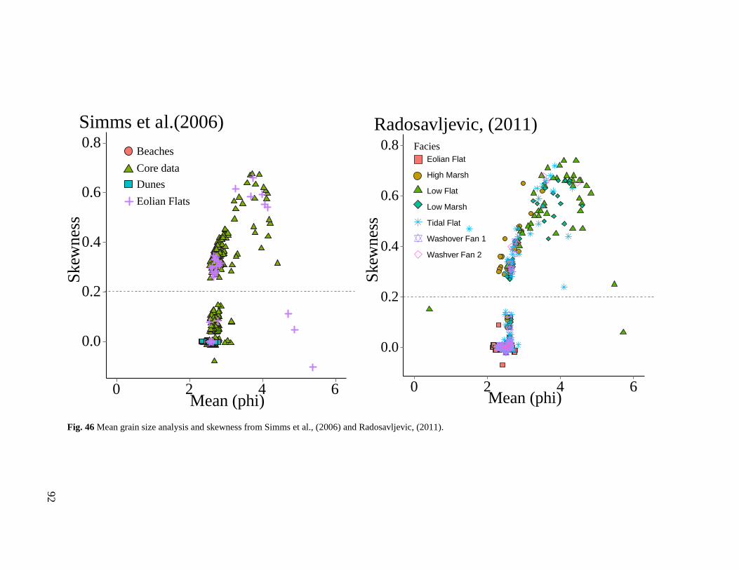
92

Fig. 46 Mean grain size analysis and skewness from Simms et al., (2006) and Radosavljevic, (2011).

0.0

0.2

0.4

0.6

0.8

0 2 4 6Mean (phi)

Skew

nes

s

Beaches

Core data

Dunes

Eolian Flats

Simms et al.(2006)

0.0

0.2

0.4

0.6

0.8

0 2 4 6Mean (phi)

Skew

nes

s

Facies

Eolian Flat

High Marsh

Low Flat

Low Marsh

Tidal Flat

Washover Fan 1

Washver Fan 2

Radosavljevic, (2011)

93

Fig. 47 Mean grain size analysis and skewness for this study.

Sediment Plate Technique

The advantages of using sediment plates is that they are easy to install, are

more robust and are less likely to be interrupted by erosion. Sediment plates are

ideal for areas that do not experience significant erosion, such as the high marsh

region. Disadvantages include: sediment plates allow for only one measurement

when the sediment is removed for analysis.

0.0

0.2

0.4

0.6

0.8

0 2 4 6Mean (phi)

Skew

nes

s

High Marsh

High Tidal Flat

Low Marsh

Low Tidal Flat

This Study

94

Conclusion

In general aeolian sediment transport is a significant mechanism for

sediment deposition on marsh surfaces further from tidal creeks. Two windy

events produced elevated deposition rates of greater than 2cm and contributing

ten times as much accretion than occurs in one year. Although the deposition was

highly episodic across the marsh, sediment deposition correlated well with

number of flooding events, and duration for plates near the main tidal creek. The

total accumulation deposited on plates was dominated by inorganic sediments,

suggesting there is a limit of detrital organic matter contribution for this area.

95

References

Barbier, E.B., S.D. Hacker, C. Kennedy, E.W. Koch, A.C. Stier, and B.R. Silliman. 2010.

The value of estuarine and coastal ecosystem services. Ecological Monographs

81: 169–193. doi:10.1890/10-1510.1.

Baustian, Joseph J., and Irving A. Mendelssohn. 2015. Hurricane-Induced Sedimentation

Improves Marsh Resilience and Vegetation Vigor under High Rates of Relative

Sea Level Rise. Wetlands 35: 795–802. doi:10.1007/s13157-015-0670-2.

Bertness, M.D. 1991. Zonation of Spartina patens and Spartina alterniflora in New

England salt marsh. Ecology 72: 138–148.

Blake, W. H, D. E Walling, and Q He. 1999. Fallout beryllium-7 as a tracer in soil

erosion investigations. Applied Radiation and Isotopes 51: 599–605.

doi:10.1016/S0969-8043(99)00086-X.

Bricker-Urso, S., S. W. Nixon, J. K. Cochran, D. J. Hirschberg, and C. Hunt. 1989.

Accretion rates and sediment accumulation in Rhode Island salt marshes.

Estuaries 12: 300–317. doi:10.2307/1351908.

Brinson, M.M. 1993. A hydrogeomorphic classification for wetlands. U.S. Army Corps

of Engineers.

Brinson, M.M., R.R. Christian, and L.K. Blum. 1995. Multiple states in the sea-level

induced transition from terrestrial forest to estuary. Estuaries 18: 648–659.

Cahoon, Donald R., Philippe F. Hensel, Tom Spencer, Denise J. Reed, Karen L. McKee,

and Neil Saintilan. 2006. Coastal Wetland Vulnerability to Relative Sea-Level

Rise: Wetland Elevation Trends and Process Controls. In Wetlands and Natural

Resource Management, ed. Prof Dr Jos T. A. Verhoeven, Dr Boudewijn Beltman,

Dr Roland Bobbink, and Dr Dennis F. Whigham, 271–292. Ecological Studies

190. Springer Berlin Heidelberg.

Cahoon, Donald R., and James C. Lynch. 1997. Vertical accretion and shallow

subsidence in a mangrove forest of southwestern Florida, U.S.A. Mangroves and

Salt Marshes 1: 173–186. doi:10.1023/A:1009904816246.

Cahoon, D.R. 1997. Global Warming, Sea-level Rise, and Coastal Marsh Survival USGS

FS-091-97. US Department of the Interior, US Geological Survey.

Cahoon, D. R., and D. J. Reed. 1995. Relationships among Marsh Surface Topography,

Hydroperiod, and Soil Accretion in Deteriorating Louisiana Salt Marsh. Journal

of Coastal Research 11: 357–369.

Cahoon, D.R., D.J. Reed, and J.W. Day. 1995. Estimating shallow subsidence in

microtidal salt marshes of the southeastern United States: Kaye and Barghoorn

revisited. Marine Geology 128: 1–9. doi:10.1016/0025-3227(95)00087-F.

Cahoon, D.R., and R.E. Turner. 1989. Accretion and canal impacts in a rapidly subsiding

wetland II. Feldspar marker horizon technique. Estuaries 12: 260–268.

Callaway, J.C., R.D. DeLaune, and W.H. Patrick Jr. 1997. Sediment accretion rates from

four coastal wetlands along the Gulf of Mexico. Journal of Coastal Research 13:

181–191.

Callaway, J.C., J.A. Nyman, and R.D. DeLaune. 1996. Sediment accretion in coastal

wetlands: A review and a simulation model of processes. Current Topics in

Wetland Biogeochemistry 2: 2–23.

96

Costanza, R., R. d’Arge, R. de Groot, S. Farber, M. Grasso, B. Hannon, K. Limburg, et

al. 1997. The value of the world’s ecosystem services and natural capital. Nature

387: 253–260. doi:10.1038/387253a0.

DeLaune, R. D., R. H. Baumann, and J. G. Gosselink. 1983. Relationships Among

Vertical Accretion, Coastal submergence, and Erosion in a Louisiana Gulf Coast

Marsh. Journal of Sedimentary Research 53: 147–157.

Finlayson, C. M, R. D’Cruz, N. Davidson, and World Resources Institute Millennium

Ecosystem Assessment (Program). 2005. Ecosystems and human well-being:

wetlands and water : synthesis. Washington, D.C.: World Resources Institute.

Folk, R. L. 1974. Petrology of Sedimentary Rocks. Austin, TX: Hemphill Publishing

Company.

Frantz, C. M., V. A. Petryshyn, and F. A. Corsetti. 2015. Grain trapping by filamentous

cyanobacterial and algal mats: implications for stromatolite microfabrics through

time. Geobiology 13: 409–423. doi:10.1111/gbi.12145.

Frey, R.W., P.B. Basan, and R.A. Davis. 1985. Coastal salt marshes. In Coastal

Sedimentary Environments, 2nd ed., 225–301. New York: Springer Verlag.

Gibeaut, J.C. 2007. Modeling future coastal wetland transition induced by relative sea‐level rise. In Proceedings of the Sixth International Symposium on Coastal

Engineering and Science of Coastal Sediment Processes. New Orleans,

Louisiana: American Society of Civil Engineers. doi:10.1061/40926(239)92.

Gibeaut, J.C., E. Barraza, and B. Radosavljevic. 2010. Estuarine wetland habitat

transition induced by relative sea-level rise on Mustang and North Padre Islands,

Texas: Phase I. Prepared for Coastal Bend Bays and Estuaries Program.

Publication CBBEP-64, Project Number-0822.

Gibeaut, J.C., T.A. Tremblay, and T.L. Hepner. 2008. Geo-environments of Mustang

Island and North Padre Island, Texas: Status, trends, and environmental

management of a barrier-island system. In 2008 AAPG Annual Convention. San

Antonio, Texas.

Gibeaut, J.C., W.A. White, R.C. Smyth, J.R. Andrews, T.A. Tremblay, R. Gutiérrez, T.L.

Hepner, and A. Neuenschwander. 2003. Topographic variation of barrier island

subenvironments and associated habitats. In Coastal Sediments, 3:18–23.

Goodman, J.E., M.E. Wood, and W. R. Gehrels. 2007. A 17-yr record of sediment

accretion in the salt marshes of Maine (USA). Marine Geology 242: 109–121.

Gosselink, J.G., and R.E. Turner. 1978. The role of hydrology in freshwater wetland

ecosystems. In Freshwater wetlands: ecological processes and management

potential, ed. R. E. Good, D. F. Whigham, and R. L. Simpson. Academic Press.

HOBO Onset. 2015. Water Level Logger.

Kleiss, B. 1993. Methods for Measuring Sedimentation Rates in Bottomland Hardwood

(BLH) Wetlands. WRP Technical Note SD-CP-4.1. Vicksburg, MS, USA: U.S.

Army Engineer Waterways Experiment Station.

Knaus, R. M., and D. L. Van Gent. 1989. Accretion and canal impacts in a rapidly

subsiding wetland. III. A new soil horizon marker method for measuring recent

accretion. Estuaries 12: 269–283.

Landau, Herbert, Ulrich Vollath, and Xiaoming Chen. 2002. Virtual Reference Station

Systems. Journal of Global Positioning Systems 01: 137–143.

97

McCaffrey, R., and J. Thompson. 1980. A record of the accumulation of sediment and

trace metals in a Connecticut salt marsh. Advances in Geophysics 22: 165–236.

McLachlan, Anton, and Ian Turner. 1994. The Interstitial Environment of Sandy

Beaches. Marine Ecology 15: 177–212. doi:10.1111/j.1439-0485.1994.tb00053.x.

Mitsch, W.J., and J.G. Gosselink. 2000. Wetlands. 3rd Edition. Columbus, Ohio: John

Wiley & Sons.

Montagna, P.A., J.C. Gibeaut, and J.W. Tunnell. 2007. South Texas climate 2100:

Coastal impacts. In South Texas Climate 2100: Problems and Prospects, Impacts

and Implications, ed. W. Norwine and K. John. Texas A&M University -

Kingsville.

Morton, R. A. 1988. Interactions of Storms, Seawalls, and Beaches of the Texas Coast.

Journal of Coastal Research: 113–134.

Morton, R.A., and J.H. McGowen. 1980. Modern depositional environments of the Texas

coast. Austin, Texas: Bureau of Economic Geology, Guidebook 20: 167 p.

Moulton, Daniel W., and John S. Jacob. 2000. Texas Coastal Wetlands Guidebook.

TAMU-SG. Texas Sea Grant College Program.

Neubauer, S.C., I.C. Anderson, J.A. Constantine, and S.A. Kuehl. 2002. Sediment

deposition and accretion in a mid-Atlantic (U.S.A.) tidal freshwater marsh.

Estuarine, Coastal and Shelf Science 54: 713–727. doi:10.1006/ecss.2001.0854.

NOAA. 2012. Fisheries Economics of the U.S. 2012. Regional Summary FEUS 2012.

Gulf of Mexico: NOAA, National Marine Fisheries Service.

NOAA. 2014a. Mean Sea Level Trends. Government. Tides & Currents.

NOAA. 2014b. Hurricanes. Web Portal. Historical Hurricane Tracks.

NOAA. 2015. National Weather Service.

Nolte, S., E.C. Koppenaal, P. Esselink, K.S. Dijkema, M. Schuerch, A.V. De Groot, J.P.

Bakker, and S. Temmerman. 2012. Measuring sedimentation in tidal marshes: a

review on methods and their applicability in biogeomorphological studies.

Journal of Coastal Conservation 16.

OTT Orpheus Mini. 2015. Water Level Logger.

Paine, J. G., W. A. White, J. C. Gibeaut, J. R. Andrews, and R. Waldinger. 2004.

Exploring Quantitative Wetlands Mapping Using Airborne Lidar and

Electromagnetic Induction on Mustang Island, Texas. AGU Spring Meeting

Abstracts -1: 24.

Paine, J.G., W.A. White, R.C. Smyth, J.R. Andrews, and J.C. Gibeaut. 2004. Mapping

coastal environments with lidar and EM on Mustang Island. The Leading Edge

23: 894–98.

Paquette, Cynthia H., Karen L. Sundberg, Roelof M. J. Boumans, and Gail L. Chmura.

2004. Changes in saltmarsh surface elevation due to variability in

evapotranspiration and tidal flooding. Estuaries 27: 82–89.

doi:10.1007/BF02803562.

Parkinson, Randall W., Ron D. DeLaune, and John R. White. 1994. Holocene Sea-Level

Rise and the Fate of Mangrove Forests Within the Wider Caribbean Region.

Journal of Coastal Research 10: 1077–1086.

Perillo, Gerardo M. E., Eric Wolanski, Donald R. Cahoon, and Mark M. Brinson. 2009.

Coastal Wetlands: An Integrated Ecosystems Approach. First. Amsterdam, The

Netherlands: Elsevier.

98

Pethick, J.S. 1981. Long-term accretion rates on tidal salt marshes. Journal of

Sedimentary Research 51: 571–577.

Petovello, M. 2011. Inside GNSS Engineering Solutions from the Global Navigation

Satellite System Community, July.

Pulich, Warren Jr., Catherine Blair, and William A. White. 1997. Current Status and

Historical Trends of Seagrass in the Corpus Christi Bay National Estuary

Program Study Area. CCBNEP-20. Bureau of Economic Geology, Jackson

School of Geosciences, The University of Texas at Austin.

Radosavljevic, Boris. 2011. Vertical accretion rates in microtidal wetlands and sea-level

rise: Mustang Island, TX. Thesis, Texas A&M University - Corpus Christi.

Reed, D.J. 1989. Patterns of sediment deposition in subsiding coastal salt marshes,

Terrebonne Bay, Louisiana: the role of winter storms. Estuaries 12: 222–227.

Reed, D.J., and D.R. Cahoon. 1992. The relationship between marsh surface topography,

hydroperiod, and growth of Spartina alterniflora in a deteriorating Louisiana salt

marsh. Journal of Coastal Research 8: 77–87.

Reed, D.J., and D.R. Cahoon. 1993. Marsh submergence vs. marsh accretion: Interpreting

accretion deficit data in coastal Louisiana. In Coastal Zone ’93, 243–257. New

Orleans, LA: ASCE.

Shaffer, Juliet P. 1986. Modified Sequentially Rejective Multiple Test Procedures.

Journal of the American Statistical Association 81: 826–831.

Shaler, N. S. 1886. Preliminary report on seacoast swamps of the Eastern United States.

Washington, D.C., U.S.A.: US Geologic Survey.

Shepard, F. P. 1954. Nomenclature based on sand-silt-clay ratios. Journal of Sedimentary

Petrology 24: 151–158.

Shideler, G.L. 1984. Suspended sediment responses in a wind-dominated estuary of the

Texas Gulf Coast. Journal of Sedimentary Research 54: 731–745.

doi:10.1306/212F84E5-2B24-11D7-8648000102C1865D.

Simms, A.R., J.B. Anderson, and M. Blum. 2006. Barrier-island aggradation via inlet

migration: Mustang Island, Texas. Sedimentary Geology 187: 105–125.

Stevenson, J.C., L.G. Ward, and M.S. Kearney. 1985. Vertical accretion in marshes with

varying rates of sea level rise. In Estuaries, 8:241–259.

Stumpf, R.P. 1983. The process of sedimentation on the surface of a salt marsh.

Estuarine, Coastal and Shelf Science 17: 495–508.

Swenson, Erick M., and R. E. Turner. 1987. Spoil banks: Effects on a coastal marsh

water-level regime. Estuarine, Coastal and Shelf Science 24: 599–609.

doi:10.1016/0272-7714(87)90101-6.

Thomas, Séverine, and Peter V Ridd. 2004. Review of methods to measure short time

scale sediment accumulation. Marine Geology 207: 95–114.

doi:10.1016/j.margeo.2004.03.011.

Turner, R.E., E.M. Swenson, and C.S. Milan. 2002. Organic and inorganic contributions

to vertical accretion in salt marsh sediments. Concepts and Controversies in Tidal

Marsh Ecology: 583–595.

Westfall, Peter H. 1997. Multiple testing of general contrasts using logical constraints

and correlations. Journal of the American Statistical Association 92: 299–306.

99

White, W.A., R.A. Morton, and C.W. Holmes. 2001. A comparison of factors controlling

sedimentation rates and wetland loss in fluvial-deltaic systems, Texas Gulf coast.

Geomorphology 44: 47–66.

White, W.A., R.A. Morton, R.S. Kerr, W.D. Kuenzi, and W.B. Brogden. 1978. Land and

water resources, historical changes, and dune criticality: Mustang and North

Padre Islands, Texas. Austin: Bureau of Economic Geology, The University of

Texas at Austin.

White, W.A., T.A. Tremblay, R.L. Waldinger, and T.R. Calnan. 2006. Status and trends

of wetland and aquatic habitats on Texas barrier islands Coastal Bend. Bureau of

Economic Geology, The University of Texas at Austin.

Wood, Nathan, and Albert C. Hine. 2007. Spatial Trends in Marsh Sediment Deposition

Within a Microtidal Creek System, Waccasassa Bay, Florida. Journal of Coastal

Research: 823–833. doi:10.2112/04-0243.1.

Zuur, Alain F., Elena N. Ieno, Neil J. Walker, and Graham M. Saveliev. 2009. Mixed

Effects Models and Extensions in Ecology with R. Springer Science & Business

Media.