Case Study

Hydrologic Effects of Size and Location ofFields Converted from Drained Pine Forest

to Agricultural CroplandHyun Woo Kim1; Devendra M. Amatya2; George M. Chescheir3;

Wayne R. Skaggs4; and Jami E. Nettles5

Abstract: Hydrological effects of land-use change are of great concern to ecohydrologists and watershed managers, especially in theAtlantic coastal plain of the southeastern United States. The concern is attributable to rapid population growth and the resulting pressureto develop forested lands. Many researchers have studied these effects in various scales, with varying results. An extended watershed-scaleforest hydrologic model, calibrated with 1996–2000 data, was used to evaluate long-term hydrologic effects of conversion to agriculture(corn–wheat–soybean cropland) of a 29.5-km2 intensively managed pine-forested watershed in Washington County in eastern NorthCarolina. Fifty years of weather data (1951–2000) from a nearby weather station were used for simulating hydrology to evaluate effectson outflows, evapotranspiration, and water table depth compared with the baseline scenario. Other simulation scenarios were created foreach of five different percentages (10, 25, 50, 75, and 100%) of land-use conversion occurring at upstream and downstream locations in thepine-forest watershed. Simulations revealed that increased mean annual outflow was significant (α ¼ 0.05) only for 100% conversion fromforest (261 mm) to agricultural crop (326 mm), primarily attributed to a reduction in evapotranspiration. Although high flow rates>5 mmday−1 increased from 2.3 to 2.6% (downstream) and 2.6 to 4.2% (upstream) for 25 to 50% conversion, the frequency was higherfor the upstream location than the downstream. These results were attributed to a substantial decrease in soil hydraulic conductivity of one ofthe dominant soils in the upstream location, which is expected after land-use conversion to agriculture. As a result, predicted subsurfacedrainage decreased, and surface runoff increased as soil hydraulic conductivity decreased for the soil upstream. These results indicate thatsoil hydraulic properties resulting from land-use conversion have a greater influence on hydrologic components than the location of landuse conversion. DOI: 10.1061/(ASCE)HE.1943-5584.0000566. © 2013 American Society of Civil Engineers.

CE Database subject headings: Land use; Hydraulic conductivity; Peak flow; Evapotranspiration; Drainage; Agriculture; Hydrologicaspects.

Author keywords: DRAINWAT; Land-use change; Soil hydraulic conductivity; Outflow; Peak flow rate; Evapotranspiration.

Introduction

In recent years there has been great concern about the effect of land-use change on flooding, watershed outflows (yields), and quality ofwaters draining from the lands into downstream (DS) water bodies

(Wilk et al. 2001; Tang et al. 2005; Thanapakpawin et al. 2007;Li et al. 2011). Land-use change may occur because of changein vegetation, such as deforestation, afforestation, urbanization,and other kinds of land development. The relationship betweencatchment vegetation type and the variability of runoff, as affectedby the impact of vegetation manipulation on evapotranspiration(ET), has important implications for sustainable water-resourcesmanagement and development (De Wit 2001).

Wilk et al. (2001) reported that deforestation increased thevolume of outflow at watershed scale in a 12,100-km2 catchmentin northeast Thailand only when runoff ratio was very low. Eventhough they reported that forest clearance increased the outflow onsmall catchments of a few hectares, they could not find any sub-stantial changes or trends in any water-balance terms as the forestarea of the large watershed decreased from 80 to 27% between1957 and 1995.

Thanapakpawin et al. (2007) reported that conversion offorested lands to agricultural lands in the upstream (US) part ofa watershed led to slightly higher annual outflows (301-mm annualaverage, 55.1-mm maximum daily flow) than those of mid- ordownstream conversion (297-mm annual average, 54.3-mm maxi-mum daily flow). After they considered the irrigation effect, themagnitude of difference was slightly greater. The annual averageoutflow was 256 mm, and the maximum daily outflow was49.6 mm for upstream conversion. For downstream conversion,

1Research Scientist, Dept. of Water Environmental EngineeringResearch, National Institute of Environmental Research, EnvironmentalResearch Complex, Kyungseo-dong, Seo-gu, Incheon 404-708, Republicof Korea. E-mail: kim4hydro@korea.kr

2Research Hydrologist, USDA Forest Service, Center for ForestedWetlands Research, 3734 Highway 402, Cordesville, SC 29434(corresponding author). E-mail: damatya@fs.fed.us

3Research Associate Professor, Dept. of Biological and AgriculturalEngineering, North Carolina State Univ., Campus Box 7625, Raleigh,NC 27695.

4William Neal Reynolds Distinguished Univ. Professor, Dept. ofBiological and Agricultural Engineering, North Carolina State Univ.,Campus Box 7625, Raleigh, NC 27695.

5Principal Scientist, Weyerhaeuser Company, P.O. Box 2288,Columbus, MS 39704.

Note. This manuscript was submitted on November 8, 2010; approvedon December 28, 2011; published online on January 2, 2012. Discussionperiod open until October 1, 2013; separate discussions must be submittedfor individual papers. This paper is part of the Journal of Hydrologic En-gineering, Vol. 18, No. 5, May 1, 2013. © ASCE, ISSN 1084-0699/2013/5-552-566/$25.00.

552 / JOURNAL OF HYDROLOGIC ENGINEERING © ASCE / MAY 2013

J. Hydrol. Eng. 2013.18:552-566.

Dow

nloa

ded

from

asc

elib

rary

.org

by

Nor

th C

arol

ina

Stat

e U

nive

rsity

on

04/2

9/13

. Cop

yrig

ht A

SCE

. For

per

sona

l use

onl

y; a

ll ri

ghts

res

erve

d.

these values decreased to 235 mm for annual mean outflow and46.5 for maximum daily outflow.

It is well known that land-use change influences the hydrology[primarily through changes in ET, surface, and subsurface flow,as affected by water table depth (WTD)] and biogeochemistry ofwatersheds. As land-use changes from unaltered natural landscapessuch as forests and wetlands to agricultural and urban areas, surfacerunoff (SRO) and anthropogenic chemical and wastewater inputsalmost always increase (Tong and Chen 2002; Fitzpatrick et al.2007; Qi et al. 2009). Physical alteration of the landscape attribut-able to land-use change also affects the hydrogeologic dynamics ofwatersheds (Tang et al. 2005).

The effects of land-use change in the Atlantic and Gulf Coastregions of the United States are of even greater concern becauseof rapid growth in population and increased pressure to developforested lands, most of which are in proximity to ecologically sen-sitive waters. It seems likely that demand for increased agriculturalproduction to feed a rapidly expanding global population, coupledwith current high commodity prices, will lead to increased conver-sion of forested lands to agriculture. The need to produce biofuel-based crops like switchgrass will potentially add to the pressure forconversion. Converting forested lands to the production of agricul-tural crops nearly always reduces ET and increases runoff (Skaggset al. 1991, 2011; Sun et al. 2005; Amatya et al. 2008; Amatya andTrettin 2007).

Recent experimental studies conducted in North Carolinacoastal plain watersheds (Fig. 1) compared the average annual run-off and its temporal distribution from agricultural lands with those

from pine forest (Shelby et al. 2005; Amatya et al. 2002). Theyfound an almost twofold-higher average annual runoff fromagricultural lands than from forested sites. However, less such in-formation is known on hydrologic effects of size and location ofland conversion within a watershed. Land managers and regulatoryagencies often need this information to evaluate actual effects ofland-use changes.

Long-term measurements to examine such effects are cost-prohibitive in most cases; therefore, watershed-scale hydrologicand water-quality models are frequently used to simulate effects ofland-use change and management scenarios (Weber et al. 2001; Sunet al. 2005; Fernandez et al. 2007; Gassman et al. 2007; Amatyaet al. 2008, 2011). In recent years, several different types of modelshave been developed and applied to estimate the effects of land-useconversion [a conceptual rainfall-runoff model by Nandakumar andMein (1997); Hydrologiska Byrans Vattenbalans-avdeling (HBV)model by Wilk et al. (2001); BASINS by Tong and Chen (2002);DRAINMOD by Skaggs et al. (2011); LTM and L-THIA by Tanget al. (2005); DHSVM by Thanapakpawin et al. (2006); IBIS andTHIMB by Li et al. (2007); and MODFLOW and HSPF by Choet al. (2009)]. Recently, Qi et al. (2009) used the USGS PRMSmodel to evaluate streamflow response to climate and land-usechanges in coastal North Carolina. The authors reported a 14–20%increase in streamflow as a result of converting forest, which madeup 69% of their 377-km2 watershed, to agricultural crops. Only afew models are capable of reliably simulating the hydrology ofpoorly drained soils, especially in low-gradient forested landscapes.One such model is DRAINMOD (Skaggs 1978), a process-based

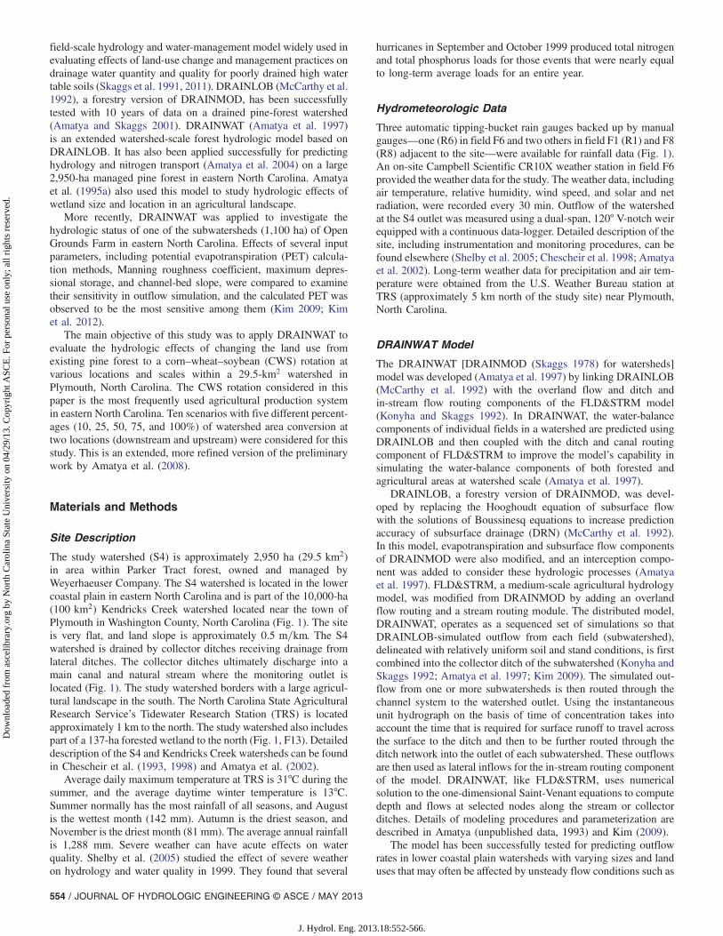
Fig. 1. Location map and layout of forested watershed near Plymouth, North Carolina

JOURNAL OF HYDROLOGIC ENGINEERING © ASCE / MAY 2013 / 553

J. Hydrol. Eng. 2013.18:552-566.

Dow

nloa

ded

from

asc

elib

rary

.org

by

Nor

th C

arol

ina

Stat

e U

nive

rsity

on

04/2

9/13

. Cop

yrig

ht A

SCE

. For

per

sona

l use

onl

y; a

ll ri

ghts

res

erve

d.

field-scale hydrology and water-management model widely used inevaluating effects of land-use change and management practices ondrainage water quantity and quality for poorly drained high watertable soils (Skaggs et al. 1991, 2011). DRAINLOB (McCarthy et al.1992), a forestry version of DRAINMOD, has been successfullytested with 10 years of data on a drained pine-forest watershed(Amatya and Skaggs 2001). DRAINWAT (Amatya et al. 1997)is an extended watershed-scale forest hydrologic model based onDRAINLOB. It has also been applied successfully for predictinghydrology and nitrogen transport (Amatya et al. 2004) on a large2,950-ha managed pine forest in eastern North Carolina. Amatyaet al. (1995a) also used this model to study hydrologic effects ofwetland size and location in an agricultural landscape.

More recently, DRAINWAT was applied to investigate thehydrologic status of one of the subwatersheds (1,100 ha) of OpenGrounds Farm in eastern North Carolina. Effects of several inputparameters, including potential evapotranspiration (PET) calcula-tion methods, Manning roughness coefficient, maximum depres-sional storage, and channel-bed slope, were compared to examinetheir sensitivity in outflow simulation, and the calculated PET wasobserved to be the most sensitive among them (Kim 2009; Kimet al. 2012).

The main objective of this study was to apply DRAINWAT toevaluate the hydrologic effects of changing the land use fromexisting pine forest to a corn–wheat–soybean (CWS) rotation atvarious locations and scales within a 29.5-km2 watershed inPlymouth, North Carolina. The CWS rotation considered in thispaper is the most frequently used agricultural production systemin eastern North Carolina. Ten scenarios with five different percent-ages (10, 25, 50, 75, and 100%) of watershed area conversion attwo locations (downstream and upstream) were considered for thisstudy. This is an extended, more refined version of the preliminarywork by Amatya et al. (2008).

Materials and Methods

Site Description

The study watershed (S4) is approximately 2,950 ha (29.5 km2)in area within Parker Tract forest, owned and managed byWeyerhaeuser Company. The S4 watershed is located in the lowercoastal plain in eastern North Carolina and is part of the 10,000-ha(100 km2) Kendricks Creek watershed located near the town ofPlymouth in Washington County, North Carolina (Fig. 1). The siteis very flat, and land slope is approximately 0.5 m=km. The S4watershed is drained by collector ditches receiving drainage fromlateral ditches. The collector ditches ultimately discharge into amain canal and natural stream where the monitoring outlet islocated (Fig. 1). The study watershed borders with a large agricul-tural landscape in the south. The North Carolina State AgriculturalResearch Service’s Tidewater Research Station (TRS) is locatedapproximately 1 km to the north. The study watershed also includespart of a 137-ha forested wetland to the north (Fig. 1, F13). Detaileddescription of the S4 and Kendricks Creek watersheds can be foundin Chescheir et al. (1993, 1998) and Amatya et al. (2002).

Average daily maximum temperature at TRS is 31°C during thesummer, and the average daytime winter temperature is 13°C.Summer normally has the most rainfall of all seasons, and Augustis the wettest month (142 mm). Autumn is the driest season, andNovember is the driest month (81 mm). The average annual rainfallis 1,288 mm. Severe weather can have acute effects on waterquality. Shelby et al. (2005) studied the effect of severe weatheron hydrology and water quality in 1999. They found that several

hurricanes in September and October 1999 produced total nitrogenand total phosphorus loads for those events that were nearly equalto long-term average loads for an entire year.

Hydrometeorologic Data

Three automatic tipping-bucket rain gauges backed up by manualgauges—one (R6) in field F6 and two others in field F1 (R1) and F8(R8) adjacent to the site—were available for rainfall data (Fig. 1).An on-site Campbell Scientific CR10X weather station in field F6provided the weather data for the study. The weather data, includingair temperature, relative humidity, wind speed, and solar and netradiation, were recorded every 30 min. Outflow of the watershedat the S4 outlet was measured using a dual-span, 120° V-notch weirequipped with a continuous data-logger. Detailed description of thesite, including instrumentation and monitoring procedures, can befound elsewhere (Shelby et al. 2005; Chescheir et al. 1998; Amatyaet al. 2002). Long-term weather data for precipitation and air tem-perature were obtained from the U.S. Weather Bureau station atTRS (approximately 5 km north of the study site) near Plymouth,North Carolina.

DRAINWAT Model

The DRAINWAT [DRAINMOD (Skaggs 1978) for watersheds]model was developed (Amatya et al. 1997) by linking DRAINLOB(McCarthy et al. 1992) with the overland flow and ditch andin-stream flow routing components of the FLD&STRM model(Konyha and Skaggs 1992). In DRAINWAT, the water-balancecomponents of individual fields in a watershed are predicted usingDRAINLOB and then coupled with the ditch and canal routingcomponent of FLD&STRM to improve the model’s capability insimulating the water-balance components of both forested andagricultural areas at watershed scale (Amatya et al. 1997).

DRAINLOB, a forestry version of DRAINMOD, was devel-oped by replacing the Hooghoudt equation of subsurface flowwith the solutions of Boussinesq equations to increase predictionaccuracy of subsurface drainage (DRN) (McCarthy et al. 1992).In this model, evapotranspiration and subsurface flow componentsof DRAINMOD were also modified, and an interception compo-nent was added to consider these hydrologic processes (Amatyaet al. 1997). FLD&STRM, a medium-scale agricultural hydrologymodel, was modified from DRAINMOD by adding an overlandflow routing and a stream routing module. The distributed model,DRAINWAT, operates as a sequenced set of simulations so thatDRAINLOB-simulated outflow from each field (subwatershed),delineated with relatively uniform soil and stand conditions, is firstcombined into the collector ditch of the subwatershed (Konyha andSkaggs 1992; Amatya et al. 1997; Kim 2009). The simulated out-flow from one or more subwatersheds is then routed through thechannel system to the watershed outlet. Using the instantaneousunit hydrograph on the basis of time of concentration takes intoaccount the time that is required for surface runoff to travel acrossthe surface to the ditch and then to be further routed through theditch network into the outlet of each subwatershed. These outflowsare then used as lateral inflows for the in-stream routing componentof the model. DRAINWAT, like FLD&STRM, uses numericalsolution to the one-dimensional Saint-Venant equations to computedepth and flows at selected nodes along the stream or collectorditches. Details of modeling procedures and parameterization aredescribed in Amatya (unpublished data, 1993) and Kim (2009).

The model has been successfully tested for predicting outflowrates in lower coastal plain watersheds with varying sizes and landuses that may often be affected by unsteady flow conditions such as

554 / JOURNAL OF HYDROLOGIC ENGINEERING © ASCE / MAY 2013

J. Hydrol. Eng. 2013.18:552-566.

Dow

nloa

ded

from

asc

elib

rary

.org

by

Nor

th C

arol

ina

Stat

e U

nive

rsity

on

04/2

9/13

. Cop

yrig

ht A

SCE

. For

per

sona

l use

onl

y; a

ll ri

ghts

res

erve

d.

backwater effects (Konyha and Skaggs 1992; Amatya et al. 1997).A detailed sensitivity analysis of both the field hydrology andditch/canal routing parameters for flow in canals and streams wasconducted by Konyha and Skaggs (1992), Kim (2009), and Kimet al. (2012). Diggs (2004) used a similar approach (DRAINMODwith Penman–Monteith PET, without an interception component)to predict outflows from another drained pine-forest site in theParker Tract with good results.

The model was validated with 5 years of data (1996–2000) forpredicting the outflow rates and nitrogen transport for this studywatershed (S4) (Amatya et al. 2004). However, forest canopyevaporation caused by rainfall interception was not simulatedbecause the data on canopy storage and coverage, leaf area index(LAI), and stomatal conductance for all stands in the watershedwere not available. Instead, the Penman–Monteith PET for the for-est reference estimated using the measured daily LAI function andmaximum stomatal conductance for the pine forest with weathervariables measured above its canopy was used in DRAINMOD tosimulate ET (Amatya et al. 2004). The maximum stomatal conduct-ance value was obtained from the Carteret study site (McCarthyet al. 1992; Amatya et al. 1996). The authors showed that themodel-predicted outflows and their time distribution for 5 years(1996–2000) were in good agreement with measured data forthe watershed. Predictions correlated well with the measured data(R2 ¼ 0.90, p < 0.001). The predicted total cumulative monthlyoutflow of 1,554 mm at the end of the 5-year period was only4 mm higher than the measured amount of 1,550 mm. The averageabsolute monthly deviation varied from 5 mm in 1997 to 11.8 mmin 1998 (average ¼ 8.2 mm), and the yearly Nash–Sutcliffe coef-ficient ranged from 0.79 to 0.91 (average ¼ 0.89), which is con-sidered good on the basis of criteria recently developed (Moriasiet al. 2007). These analyses indicate that the model adequatelydescribes daily and monthly drainage outflows for the study water-shed. The fact that the average rainfall of 1,249 mm for the-5-yearperiod was only 3% lower than that for the 50-year period simu-lated, and the mean outflow of 263 mm for the same period wasalso close to the 50-year average of 261 mm as will be shown later,further indicates that the calibrated model captures the average base-line hydrological conditions of the 50-year period. The validatedmodel was applied in this paper to evaluate the hydrologic effectsof conversion of the current pine forest into agricultural crop.

Modeling Scenarios

At first, a baseline scenario with all 27 fields (subwatersheds delin-eated for the S4 watershed) (Fig. 2) in their existing condition(all pine forest) was simulated. The results on hydrology (outflowfor the whole watershed, ET, water table depth) were saved forthis baseline scenario. Five other hypothetical scenarios involvingthe conversion of approximately 10, 25, 50, 75, and 100% of the2,950-ha pine forest to a CWS crop rotation were simulated.

Further simulation scenarios were created for each of these per-centages of land-use change occurring at upstream and downstreamlocations of the watershed. Fig. 2 is a sample schematic layout forconversion of 25% upstream [Fig. 2(a)] and 50% downstream[Fig. 2(b)] of the watershed. Fields were selected arbitrarily (visualbasis) to obtain the desired percentage conversion for upstream anddownstream portions of the watershed. Altogether, 10 sets of modelsimulations were conducted using a 51-year (1950–2000), long-term weather data set obtained from the U.S. Weather BureauStation at Plymouth, North Carolina. The simulation of the firstyear (1950) was used to define initial conditions for January 1,1951, so results for that year were not used in the analysis. Thescenarios considered were summarized and tabulated in Table 1.

Model Parameterization for This Study

Hydrologic effects of conversion from original pine forest to theagricultural crop rotation were simulated by changing soil hy-draulic properties, surface storage, rooting depth, and the referenceET (REF-ET) (or PET) for the forest fields to values consistent withagricultural crops (Table 2).

Drainage Design Parameters

The individual fields of the watershed are drained by lateral ditchesthat are 0.6–1.2 m deep and mostly 100 m apart. The lateral ditchesdischarge to collector ditches 1.8–2.5 m deep and 800 m apart(Fig. 3); these ditches, in turn, discharge to main canals, which are1.8–3.0 m deep, and then finally to the natural stream. Bed slopewas 0.5 m=km, and Manning roughness coefficients ranged from0.035 (upstream) to 0.050 (downstream) for baseline simulation.These values remained the same for both the baseline and theconversion scenarios for earthen ditches and canals.

Fig. 2. Examples of field diagram (not to scale): (a) 25% upstream; (b) 50% downstream

JOURNAL OF HYDROLOGIC ENGINEERING © ASCE / MAY 2013 / 555

J. Hydrol. Eng. 2013.18:552-566.

Dow

nloa

ded

from

asc

elib

rary

.org

by

Nor

th C

arol

ina

Stat

e U

nive

rsity

on

04/2

9/13

. Cop

yrig

ht A

SCE

. For

per

sona

l use

onl

y; a

ll ri

ghts

res

erve

d.

Table 1. Spatial Distribution of Land-Use Conversion within 2,950 Ha for Various Scenarios

Conversion toagriculturalcropland (%) Location Field number converted to agricultural cropland Area (ha)

Percent ofwatershed

area

10 Downstream 18, 19, 26 267 9.1Upstream 1, 3, 8 301 10.2

25 Downstream 18, 19, 26, 21, 22, 23, 24, 27 727 24.6Upstream 1, 3, 8, 2, 4, 9, 10 766 26.0

50 Downstream 18, 19, 26, 21, 22, 23, 24, 27, 12, 13, 14, 15, 16, 17, 20 1,492 50.6Upstream 1, 3, 8, 2, 4, 9, 10, 5, 6, 7, 11, 12, 25 1,493 50.6

75 Downstream 18, 19, 26, 21, 22, 23, 24, 27, 12, 13, 14, 15, 16, 17, 20, 2, 4, 8, 9, 10, 11 2,211 75.0Upstream 1, 3, 8, 2, 4, 9, 10, 5, 6, 7, 11, 12, 25, 13, 14, 15, 20, 21, 22, 23 2,187 74.1

Note: Dominant soil types [and, in parentheses, their symbols as per the SCS (1981)] that are within the fields indicated by the numbers shown in Fig. 2:Belhaven (Ba): 5, 6, 7, 10, 12, 14, 15, 16, 17, 20, 21, 22, 23, 24, 25; Cape Fear (Cf): 1, 2, 3, 4, 8, 9, 11, 18; Portsmouth (Pt): 19; Wasda (Wd): 26, 27; andPortsmouth (Pt) modified for the wetland field: 13.

Table 2. Soil Hydraulic Properties for Major Soil Types

Land use Properties

Soil types

Ba Cf Pt Wd

Impermeable layer depth (cm) 240 250 240 200Hydraulic conductivity 700 (0–30) 700 (0–30) 50 (0–30) 20 (0–30)

(cm=h) (Depth range, cm) 350 (30–45) 650 (30–40) 10 (30–50) 0.4 (30–80)10 (45–60) 100 (40–50) 10 (50–240) 1 (80–200)

Pine forest 5 (60–240) 40 (50–70)5 (70–250)

Saturated water content (cm3=cm3) 0.72 0.64 0.37 0.37Wilting point (cm3=cm3) 0.37 0.57 0.15 0.15

Rooting depth (cm) 45 45 45 45Surface storage (cm) 10.0 10.0 10.0 10.0

Impermeable layer depth (cm) 270 240 215 200Hydraulic conductivity 20 (0–30) 5 (0–36) 15 (0–30) 20 (0–30)

(cm=h) (Depth range, cm) 1 (30–80) 14 (36–42) 2 (30–100) 0.4 (30–80)Agricultural crop 0.01 (80–270) 2 (42–65) 8 (100–215) 1 (80–200)

0.1 (65–240)

Saturated water content (cm3=cm3) 0.73 0.49 0.37 0.76Wilting point (cm3=cm3) 0.45 0.17 0.17 0.45Surface storage (cm) 0.25 0.25 0.25 0.25

Note: SCS symbols: Ba ¼ Belhaven; Cf ¼ Cape Fear; Pt ¼ Portsmouth; Wd ¼ Wasda.

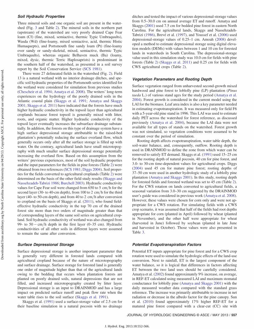
Fig. 3. Soil series classification of 10,000-ha watershed study site using ARCINFO geographic information system–based SCS soil coverage ofWashington County, North Carolina

556 / JOURNAL OF HYDROLOGIC ENGINEERING © ASCE / MAY 2013

J. Hydrol. Eng. 2013.18:552-566.

Dow

nloa

ded

from

asc

elib

rary

.org

by

Nor

th C

arol

ina

Stat

e U

nive

rsity

on

04/2

9/13

. Cop

yrig

ht A

SCE

. For

per

sona

l use

onl

y; a

ll ri

ghts

res

erve

d.

Soil Hydraulic Properties

Three mineral soils and one organic soil are present in the water-shed (Fig. 3 and Table 2). The mineral soils in the northern part(upstream) of the watershed are very poorly drained Cape Fearloam (Cf) (fine, mixed, semiactive, thermic Typic Umbraquults),Wasda (Wd) (fine-loamy, mixed semiactive, acid, thermic HisticHumaquepts), and Portsmouth fine sandy loam (Pt) (fine-loamyover sandy or sandy-skeletal, mixed, semiactive, thermic TypicUmbraquults), whereas organic Belhaven muck (Ba) (loamy,mixed, dysic, thermic Terric Haplosaprists) is predominant inthe southern half of the watershed, as presented in a soil surveyreport by the Soil Conservation Service (SCS 1981).

There were 27 delineated fields in the watershed (Fig. 2). Field13 is a natural wetland with no interior drainage ditches, and spe-cific soil hydraulic properties of the Portsmouth series identified forthe wetland were considered for simulation from previous studies(Chescheir et al. 1994; Amatya et al. 2008). The writers’ long-termexperiences on the hydrology of the poorly drained soils in theAtlantic coastal plain (Skaggs et al. 1991; Amatya and Skaggs2001; Skaggs et al. 2011) have indicated that the forests have muchhigher hydraulic conductivity in the topsoil layer than agriculturalcroplands because forest topsoil is generally mixed with litter,roots, and organic matter. Higher hydraulic conductivity of thetopsoil layer eventually increases the subsurface drainage substan-tially. In addition, the forests on this type of drainage system have ahigh surface depressional storage attributable to the raised-bedplantation’s potentially reducing the surface overland flow, whichgenerally occurs only after all the surface storage is filled up withwater. On the contrary, agricultural lands have small microtopog-raphy with much smaller surface depressional storage potentiallyincreasing the overland flow. Based on this assumption from thewriters’ previous experiences, most of the soil hydraulic propertiesand the input parameters for the fields in pine forests (Table 2) wereobtained from two references (SCS 1981; Diggs 2004). Soil proper-ties for the fields converted to agricultural croplands (Table 2) weredetermined on the basis of the other field study results (Skaggs andNassehzadeh-Tabrizi 1986; Burchell 2003). Hydraulic conductivityvalues for Cape Fear soil were changed from 650 to 5 cm=h for thesecond layer (30- to 40-cm depth), from 100 to 2 cm=h for the thirdlayer (40- to 50-cm depth), and from 40 to 2 cm=h after conversionto cropland on the basis of Skaggs et al. (2011), who found field-effective hydraulic conductivity in the top 70 cm of the drainedforest site more than two orders of magnitude greater than thatof corresponding layers of the same soil series on agricultural crop-land. Soil hydraulic conductivity of wetland was also changed from99- to 50 − cm=h depth in the first layer (0–35 cm). Hydraulicconductivities of all other soils in different layers were assumedto remain the same after conversion.

Surface Depressional Storage

Surface depressional storage is another important parameter thatis generally very different in forested lands compared withagricultural cropland because of the nature of microtopographyand surface drainage. Surface storage for forested land is generallyone order of magnitude higher than that of the agricultural landsowing to the bedding that occurs when plantation forests areplanted on poorly drained soils, natural depressions that are notfilled, and increased microtopography created by litter layer.Depressional storage is an input to DRAINMOD and has a largeimpact on predicted surface runoff and peak flow rate when thewater table rises to the soil surface (Skaggs et al. 1991).

Skaggs et al. (1991) used a surface-storage value of 2.5 cm fortheir baseline simulation in a natural pocosin with no drainage

ditches and tested the impact of various depressional-storage valuesfrom 0.5–30.0 cm on annual average ET and runoff. Amatya andSkaggs (2001) used 7.5 cm for bedded pine forest in eastern NorthCarolina. For the agricultural lands, Skaggs and Nassehzadeh-Tabrizi (1986), Brevé et al. (1997), and Youssef et al. (2006) useddepressional-storage values of 0.25–1 cm. Amoah (2008) devel-oped a method to estimate depressional storage using digital eleva-tion models (DEMs) with values between 1 and 10 cm for forestedlands in watersheds in South Carolina. The depressional-storagevalue used in this simulation study was 10.0 cm for fields with pineforests (Table 2) (Skaggs et al. 2011) and 0.25 cm for fields withCWS agricultural crops (Table 2).

Vegetation Parameters and Rooting Depth

Surface vegetation ranged from unharvested second-growth mixedhardwood and pine forest to loblolly pine (LP) plantation (Pinustaeda L.) of various stand ages for the study period (Amatya et al.2004). Forest growth is considered in the current model using theLAI for the biomass. Leaf area index is also a key parameter neededin estimating evapotranspiration. It was measured only for field F6with a 5-year-old pine stand in 1996. This LAI was used to estimatedaily PET across the watershed for forest reference, as discussedpreviously (Amatya et al. 2004), because the LAI data were notavailable for all types of stands on the watershed. Forest growthwas not simulated, so vegetation conditions were assumed to beconstant over the period of simulation.

Rooting depth affects evapotranspiration, water table depth, thesoil-water balance, and, consequently, outflow. Rooting depth isused in DRAINMOD to define the zone from which water can beremoved to satisfy ET demand. Skaggs et al. (1991) used 15–25 cmfor the rooting depth of natural pocosin, 40 cm for pine forest, and3.0- to 30-cm time-dependent values for agricultural crops. Diggs(2004) used 45 cm for mature pine forest; rooting depths of37–50 cm were used in another hydrologic study of a loblolly pineplantation (Amatya and Skaggs 2001). In this study, rooting depthfor forested fields and forested wetland was set to 45 cm (Table 2).For the CWS rotation on lands converted to agricultural fields, aseasonal variation from 3.0–30 cm suggested by the DRAINMODuser’s guide was considered in previous work (Amatya et al. 2008).However, these values were chosen for corn only and were not ap-propriate for a CWS rotation. For simulating fields with a CWScrop scenario, it was assumed that half of the fields had root depthsappropriate for corn (planted in April) followed by wheat (plantedin November), and the other half were appropriate for wheat(harvested in June) followed by soybean (planted in late Juneand harvested in October). Those values were also presented inTable 3.

Potential Evapotranspiration Factors

Potential ET inputs appropriate for pine forest and for a CWS croprotation were used to simulate the hydrologic effects of the land-useconversion. Next to rainfall, ET is the largest component of thewater balance, so it is logical that differences in factors affectingET between the two land uses should be carefully considered.Amatya et al. (2002) found approximately 9% increase, on average,in REF-ET calculated using measured LAI and maximum stomatalconductance for loblolly pine (Amatya and Skaggs 2001) with thedaily measured weather data compared with the standard grassreference. The increase was primarily attributable to increase in netradiation or decrease in the albedo factor for the pine canopy. Sunet al. (2010) found approximately 17% higher REF-ET for amatured pine forest compared with a clear-cut (CC) site with

JOURNAL OF HYDROLOGIC ENGINEERING © ASCE / MAY 2013 / 557

J. Hydrol. Eng. 2013.18:552-566.

Dow

nloa

ded

from

asc

elib

rary

.org

by

Nor

th C

arol

ina

Stat

e U

nive

rsity

on

04/2

9/13

. Cop

yrig

ht A

SCE

. For

per

sona

l use

onl

y; a

ll ri

ghts

res

erve

d.

mostly grass understory for a 2005–2007 study period. The authorsreported that the pine forest ET can be much higher than the grassREF-ET during the peak growing season.

Long-term simulations in this study used temperature-basedThornthwaite PET method (1948) because complete weather datafor using the process-based Penman–Monteith method (Monteith1965) were not available for the historic period. However, themonthly PET based on Thornthwaite method (TH PET) was ad-justed in the model using monthly correction factors calibratedwith the PET based on the Penman–Monteith method (P-M PET)from Amatya et al. (1995b, 2002) for both forested and agriculturalvegetation at this location.

Long-term (1988–2004) complete weather data measured for apine plantation forest in eastern North Carolina (Amatya et al.2006) and data from this study site for the 1996–2001 period(Amatya et al. 2004) were used to compute daily PET for thePenman–Monteith and Thornthwaite PET methods. Daily valueswere used to obtain the monthly total. Then, the monthly factorwas calculated as a ratio of the PET from the Penman–Monteithand the Thornthwaite methods (Amatya et al. 1995b). Thesemonthly factors were further used to calculate the average monthlyvalues for the pine forest. A similar procedure was followed usingthe long-term (1990–2001) data from the TRS site in Plymouth,North Carolina, for the agricultural crop–based P-M PET (Amatyaet al. 1995b, 2002). In this case, a grass reference for the shortagricultural crops was used in the P-M PET calculations.

This procedure was used because the PET rate varies dependingupon the type of reference vegetation (Sun et al. 2010). Studieshave shown that on a monthly to seasonal basis, outflow predictionsusing temperature-based Thornthwaite method with appropriatelycalibrated monthly correction factors may be as good as the methodbased on Penman–Monteith (Amatya et al. 1997, 1998; Harderet al. 2007). Interception was not simulated because leaf area indexand canopy storage data were not available for various stand typeson the watershed. Stand age of the current vegetation was alsoassumed to be constant throughout the simulation period. Themonthly factors used in TH PET for both the pine forest and agri-cultural crop were further used to estimate the weighted averagefactors on the basis of weighted area of the forest and agriculturalcrop for each percent of computed values, as shown in Table 4.

Evaluation of Hydrologic Effects

Simulation results from each of these scenarios were tabulated to-gether with the baseline scenario to evaluate the effects of size andlocation of land-use change attributable to conversion to a CWScrop rotation on the percent change of mean annual and maximumoutflow, maximum annual and minimum annual flow, mean dailyand maximum outflow rates, and their time distribution. Averageannual outflow, maximum peak flow rate, frequency and size ofvarious flow rates, average annual ET, and water table depth werealso calculated on the basis of the 50-year simulated values. Dailyrainfall, simulated flow rates, and simulated WTD were analyzed toexamine behavior of hydrology for a wet, dry, and normal year forthe baseline forested condition compared with 100% conversion toagricultural cropland, as a worst-case scenario.

Frequency and size of daily flow and daily WTD for 50 yearswere also analyzed using flow frequency duration (FDC) and WTDduration curves. Flow frequency duration, the relationship betweenmagnitude and frequency of streamflow discharges, is one of themost informative tools for showing the complete range of outflowsfrom low flows to flood events (Smakhtin 2001). It provides agraphical summary of streamflow variability at a given location,with the shape being determined by rainfall pattern, catchment size,T

able

3.VegetationRootin

gDepth

forAgriculturalCroplandon

StudiedWatershed

Dates

January1

March

26April20

April30

May

31June

22Septem

ber2

Septem

ber12

Septem

ber27

October

7October

27Novem

ber26

Decem

ber31

Rd1

a3.0

3.0

6.0

15.0

25.0

30.0

30.0

10.0

3.0

3.0

10.0

15.0

15.0

Dates

January1

February

9March

1April1

May

10May

11May

26June

5June

19July

4July

20October

27Novem

ber16

Novem

ber21

Decem

ber31

Rd2

a15.0

15.0

20.0

25.0

25.0

25.0

3.0

7.0

20.0

25.0

30.0

30.0

10.0

3.0

3.0

Note:

Rd1

¼rootingdepth1;Rd2

¼rootingdepth2.

a Monthlyrootingdepths

foragriculturalcroplandwereselected

from

DRAIN

MODuserguide(Skaggs2013),andthevalues

arethesameregardlessof

soilseries:R

d1was

assumed

corn/wheat;R

d2was

assumed

wheat/soy.

558 / JOURNAL OF HYDROLOGIC ENGINEERING © ASCE / MAY 2013

J. Hydrol. Eng. 2013.18:552-566.

Dow

nloa

ded

from

asc

elib

rary

.org

by

Nor

th C

arol

ina

Stat

e U

nive

rsity

on

04/2

9/13

. Cop

yrig

ht A

SCE

. For

per

sona

l use

onl

y; a

ll ri

ghts

res

erve

d.

physiographic characteristics of the catchment, and land use. Lowand high flow were defined first to discuss the effects of land-useconversion on daily outflow and water table depth. Low flow wasdefined as “flow that is exceeded 70% of the time” (Smakhtin2001). High flow was defined as flow that is exceeded 1–5% of thetime (Brown et al. 2005). Midflow was therefore defined as flowfrom 6–69% of the time. Tukey’s test and Student’s t-test with SAS9.1.3 (SAS Institute 2004) andMicrosoft Excel 2007 software wereused to evaluate the statistical significance of difference in simu-lated hydrologic variables between upstream and downstream sce-nario for all sizes of conversion.

Results and Discussion

Hydrologic Effects of Converting Forested Fields toAgricultural Fields

Effects of converting land use from forested to a CWS agriculturalcrop rotation are shown in Table 5.

Effects within Each Location of Conversion:Downstream and Upstream

Mean annual outflow increased with increase in the percent ofCWS cropland, as expected, for both downstream and upstreamlocations (Table 5). In the DS conversion scenario, the mean annualoutflow increased substantially, from 261 to 326 mm (19.9%), asthe percentage of conversion increased from 0 to 100%. Runoffcoefficient normalized by rainfall also increased. However, therewas no substantial difference in maximum annual and daily outflowbetween the 10 and 75% conversion (Table 5). The frequency ofzero flow rates gradually decreased from 26.9 to 14.2% for 75%conversion and then increased to 18.3% for 100% conversion toagricultural crops. In the case of the frequency of small flow rates(less than 1 mm=day), a gradual increase was found (from 49.2 to61.8%) from baseline simulation to 75% conversion, and then aslight decrease was observed from 75 to 100% conversion of water-shed area. In the case of midflow rates (1–5 mm=day), no trend wasobserved. However, the frequency of high flow rates (more than5 mm=day) gradually increased from 2.1 to 5.0% as the conversionpercentage increased from baseline simulation to 100%.

Results for conversion concentrated in the upstream locationsof the watershed were similar to those predicted for downstreamconversions (Table 5). Conversion of 50 and 75% of the forest landto cropland had a somewhat greater effect on average annual out-flow for US than for DS locations, but trends in predicted runoffstatistics were otherwise approximately the same (Table 5).

Effects within Each Percent Conversion

A 10% conversion to CWS agricultural land caused an increase inmean annual outflows of only 3.7% for DS and 4.8% for US cases,respectively. In the 10% conversion scenario, there were no signifi-cant differences in maximum annual and daily flow rates, and therewere also no unique trends in frequency of flow rates between DSand US (Table 5).

For a 25% land-use conversion from forest to agriculture, theincreases in the mean annual outflow were 9.1% for DS and 10.0%for US. Maximum annual outflow decreased 1.5% for both DS andUS conversion. The maximum daily flow rate increased only 0.1%for DS and decreased only 0.1% for US. The frequency of highflow rates >5 mmday−1 increased appreciably from 2.1% for thebaseline to 2.5% for DS and 3.0% for US scenarios, respectively.

When 50% of the forest cover was converted to CWS cropland,the mean annual outflow substantially increased (12.7% for DS and16.6% for US). The maximum annual outflow did not change forDS, however, and increased 2.7% for US. Maximum daily flowdecreased 0.1% for DS and increased 0.1% for US. The frequencyof high flow rates >5 mmday−1 increased 3.2% for DS and 4.1%for US scenarios, respectively.

The conversion of 75% from forest to CWS cropland increasedmean annual outflow by 16.4% (312 mm) for DS, and 19.4%(324 mm) for US compared with 261 mm for the baseline simu-lation results. In this percentage of land-use conversion, the maxi-mum annual outflow increased 1.1% for DS but increased 5.0% forUS. In addition, maximum daily outflows decreased 0.4% for DSand increased 0.2% for US. The frequency of high flow rates>5 mmday−1 increased 4.2% for DS and 4.7% for US scenarios,respectively.

However, the increase in mean annual outflow was significantlydifferent (Tukey’s test; α ¼ 0.05) only for 100% conversion to agri-cultural cropland (CWS), which yielded a 326-mm outflow (19.9%increase) compared with 261 mm for the baseline. When the entire

Table 4. Monthly Correction Factors for Thornthwait PET Method Used in Long-Term Simulation

MonthsEstimated forforest landa

Estimated foragricultural cropland

Estimated weighted average for various scenarios

75% agric.þ25% forest

50% agric.þ50% forest

25% agric.þ75% forest

10% agric.þ90% forest

January 2.33 2.19 2.23 2.26 2.29 2.31February 2.21 2.43 2.37 2.32 2.26 2.23March 2.15 2.19 2.18 2.17 2.16 2.15April 1.74 1.64 1.66 1.69 1.72 1.73May 1.24 1.13 1.16 1.18 1.21 1.23June 0.96 0.97 0.97 0.97 0.96 0.96July 0.91 0.85 0.87 0.88 0.90 0.91August 0.89 0.80 0.82 0.84 0.86 0.88September 0.94 0.90 0.91 0.92 0.93 0.93October 1.42 1.17 1.23 1.30 1.36 1.40November 1.67 1.19 1.31 1.43 1.55 1.62December 2.37 1.44 1.67 1.90 2.14 2.28Average 1.57 1.41 1.45 1.49 1.53 1.55

Note: agric. ¼ agricultural cropland.aThe data in column for forested land were obtained from the average of the Carteret site and Parker tract for pine forests in eastern North Carolina. The datafor agricultural land were calculated by average of Amatya et al. (1995) and 6 years of data (1996–2001) of Amatya et al. (2002) for TRS, Plymouth,North Carolina.

JOURNAL OF HYDROLOGIC ENGINEERING © ASCE / MAY 2013 / 559

J. Hydrol. Eng. 2013.18:552-566.

Dow

nloa

ded

from

asc

elib

rary

.org

by

Nor

th C

arol

ina

Stat

e U

nive

rsity

on

04/2

9/13

. Cop

yrig

ht A

SCE

. For

per

sona

l use

onl

y; a

ll ri

ghts

res

erve

d.

100% (2,950 ha) forest area was converted to CWS cropland, thesimulated maximum annual outflow increased by approximately3.5% to as much as 582 mm.

Notably, for the 10, 25, 50, and 75% land-use conversion to theCWS cropland, all outflow characteristics were somewhat greaterfor the upstream conversion scenario than for the downstream(Table 5 and Fig. 4). The dominant soil in the upstream area ofthe watershed was Cape Fear (Fig. 2, Cf). The saturated hydraulicconductivities of Cape Fear in the second (30- to 40-cm depth),third (40- to 50-cm depth), and fourth soil layer (50- to 70-cmdepth) were greatly reduced from 650 to 5 cm=h for the secondlayer, 100 to 2 cm=h for the third layer, and 40 to 2 cm=h for thefourth layer of this soil after conversion to CWS cropland (Table 2).Belhaven soil occupies most of the area of middle and downstream,and soil hydraulic conductivity also greatly decreased after conver-sion to the CWS agricultural crop rotation (Table 2). This reductionof soil hydraulic conductivity resulted in a decrease of subsurfacedrainage but increase of surface runoff. It was concluded thatdifferences in predicted effects of land-use conversion from forestto agricultural crops in the upstream and downstream locations inthis watershed were mainly attributable to projected changes inhydraulic properties of the Cape Fear and Belhaven soils.

As presented in Fig. 4, for example, mean annual surface runoffwas greater in 50% upstream conversion (120.0 mm) than in 50%downstream conversion (104.8 mm) to CWS agricultural crop[Fig. 4(a)] for all 50 years (1951–2000). On the contrary, moreannual subsurface drainage was predicted for 50% downstreamconversion (248.8 mm) than for the same percentage conversionupstream (236.0 mm) [Fig. 4(b)]. Bachmair et al. (2009) investi-gated the effects of land use and land cover (LULC) on soil struc-ture and then preferential flow during infiltration through dye-tracerexperiments from five different sites with different LULC: twograssland sites, two agricultural crop sites (tilled and untilled), andone deciduous forest site. They found that preferential flow proc-esses significantly differed among sites of different LULC eventhough the soil texture from those sites was similar. Their overallconclusion was that land use affected flow processes in soils be-cause of several controlling factors, such as soil structure, surfacemicrotopography, surface cover, and topsoil matrix characteristics.These results are consistent with the recent finding of Skaggs et al.(2011), who reported zero surface runoff from forest lands becauseof high conductivity of surface layers and large surface storage.On the basis of these observations, it was assumed that the changeof soil hydraulic properties caused by land-use conversion had agreat influence first on the flow characteristics in soil and then,eventually, on the hydrologic processes, including surface runoffand subsurface drainage.

The effect of the percentage conversion of forest land to agri-cultural cropland on mean and maximum annual outflow is shownin Figs. 5(a and b) respectively, for both US and DS conversions.As expected, mean annual outflow increased as the percentage ofconversion increased. Conversion of upstream locations to agricul-tural cropland had a greater effect on mean annual outflow than thesame level of conversion at downstream locations. This indicates thatthe effects of percent conversion on outflow processes seem also tobe affected by the soil type, their properties (especially Ks, saturatedlateral hydraulic conductivity), and the location of the soil in the land-scape. The greatest difference between the upstream and the down-stream scenario was observed in 50% conversion for mean annualoutflow and in 75% conversion formaximum annual outflow (Fig. 5).The effect of conversion observed in this study was nonlinear andwas somewhat different from those analyzed by Fernandez et al.(2007), Dai et al. (2008), and Qi et al. (2009), who reported moreor less linear changes in outflow responses.T

able

5.Simulated

Average

AnnualHydrologicVariables

Based

onSize

andLocationof

Land-Use

Conversionfrom

Pine

Forest

toAgriculturalCropland

Conversion

locatio

n

Forest

lands

convertedto

agricultu

ral

cropland

(percent

of2,950ha)

Meanannual

flow

(mm)

Increase

inmeanannual

flow

(%)

Annualoutflows

Daily

outflows

Percentdays

with

daily

flow

(in18,263

days)

Maxim

umannual

flow

(mm)

Increase

inmaxim

umannual

flow

(%)

Annualrunoff

coefficient(%

)

Maxim

umdaily

flow

(mm)

Increase

inmaxim

umdaily

flow

(%)

0mm=day

0–1

mm=d

ay1–5

mm=d

ay>5mm=d

ay

Dow

nstream

0261

0.0

562

0.0

20.3

9.98

0.0

26.9

49.2

21.8

2.1

10271

3.7

564

0.4

21.0

9.98

0.0

22.2

53.5

22.0

2.3

25287

9.1

553

−1.5

22.3

9.99

0.1

20.7

53.8

23.0

2.5

50299

12.7

562

0.0

23.2

9.97

−0.1

15.4

60.2

21.2

3.2

75312

16.4

568

1.1

24.2

9.94

−0.4

14.2

61.8

19.8

4.2

100

326

19.9

582

3.5

25.3

100.2

18.3

56.5

20.2

5.0

Upstream

0261

0.0

562

0.0

20.3

9.98

0.0

26.9

49.2

21.8

2.1

10274

4.8

564

0.4

21.3

9.98

0.0

24.7

51.2

21.8

2.3

25290

10.0

553

−1.5

22.5

9.97

−0.1

22.2

53.9

20.9

3.0

50313

16.6

577

2.7

24.3

9.99

0.1

20.2

54.8

20.9

4.1

75324

19.4

592

5.0

25.2

100.2

16.4

57.5

21.4

4.7

100

326

19.9

582

3.5

25.3

100.2

18.3

56.5

20.2

5.0

560 / JOURNAL OF HYDROLOGIC ENGINEERING © ASCE / MAY 2013

J. Hydrol. Eng. 2013.18:552-566.

Dow

nloa

ded

from

asc

elib

rary

.org

by

Nor

th C

arol

ina

Stat

e U

nive

rsity

on

04/2

9/13

. Cop

yrig

ht A

SCE

. For

per

sona

l use

onl

y; a

ll ri

ghts

res

erve

d.

Effects of Full Conversion Agricultural Cropland(CWS Rotation) on Annual Water Balance

The effect of converting the forested watershed to agricultural crop-land on outflow from the watershed was discussed previously.Effects on other hydrologic components and the water balanceare considered in this section. Average annual values predictedin 50-year simulations for the two extreme scenarios of all forestand all cropland (CWS rotation) are given in Table 6 for rainfall,outflow (surface runoff plus subsurface drainage), ET, annualWTD, outflow/rainfall (O/R) ratio, and ET/rainfall ratio.

The average rainfall for 50 years was 1,288 mm and rangedfrom 907 mm in 1970 to 1,760 mm in 1989. Predicted average an-nual outflow increased from 261 mm for baseline simulation (100%forested lands) to 326 mm for 100% conversion to a CWS rotation.This was an increase of about 20% compared with the baselinescenario. This is greater than increases obtained by Qi et al. (2009)and Fernandez et al. (2007), with baseline forest coverages of 66

and 50%, respectively (the percent increases of runoff predicted inthose studies were 14% and 16%, respectively). Dai et al. (2008)evaluated the impact of converting 100% of a wetland forest to agri-cultural cropland using DHI-MIKESHE and DRAINMOD. Theypredicted a 30 and 35% increase in average annual outflow withDHI-MIKESHE and DRAINMOD, respectively. These resultsare consistent with Skaggs et al. (2011), who found approximately37% higher mean annual outflow from an agricultural site com-pared with all pine forest.

Conversion of 100% of the S4 watershed from forest to row-cropagriculture (CWS rotation) would increase the predicted runoff ratiofrom 19.6 to 24.7% (Table 5). Predicted annual outflow for thebaseline scenario ranged from 9 to 562 mm. For 100% agriculturalcropland, the predicted outflow value ranged from 92 to 582 mm.

Predicted average annual ET decreased from 1,013 to 902 mmbecause of land-use conversion. For 100% forest, annual ET rangedfrom 817 to 1,268 mm. Simulated annual ET decreased to a range

Fig. 4. (a) Surface runoff; (b) subsurface drainage: 50% US and 50% DS conversion scenario

Fig. 5. Change of (a) mean annual; (b) maximum annual outflow according to land-use change and location

Table 6. Summary of Average Hydrologic Components for 50 Years

Land use Parameters Rainfall (mm) Outflow (mm) ET (mm) WTD (cm) O=R ratio ET=rain (%)

Average 1,288.0 261.0 1,013.1 94.8 19.6 80.3All Maximum 1,759.6 561.8 1,268.0 245.7 40.9 112.1forest Minimum 907.2 8.7 817.3 41.7 0.8 60.2(baseline) SD 185.4 142.5 79.2 41.4 9.4 13.4

COV 0.14 0.55 0.08 0.44 0.48 0.17

Average 1,288.0 326.2 902.4 66.3 24.7 71.2All Maximum 1,759.6 581.9 1,161.1 112.4 37.6 93.4agriculture Minimum 907.2 91.9 690.8 32.0 9.0 54.8(100% SD 185.4 123.5 79.4 20.4 7.0 10.3conversion) COV 0.14 0.38 0.09 0.31 0.28 0.14

Note: SD = standard deviation; COV ¼ coefficient of variation.

JOURNAL OF HYDROLOGIC ENGINEERING © ASCE / MAY 2013 / 561

J. Hydrol. Eng. 2013.18:552-566.

Dow

nloa

ded

from

asc

elib

rary

.org

by

Nor

th C

arol

ina

Stat

e U

nive

rsity

on

04/2

9/13

. Cop

yrig

ht A

SCE

. For

per

sona

l use

onl

y; a

ll ri

ghts

res

erve

d.

of 691 to 1,161 mm after conversion to agricultural cropland(Table 6). This was a decrease of approximately 11% with theCWS agricultural crop compared to the baseline with all-forestscenario. In another 5-year short-term study, Amatya et al. (2002)found 22.5% lower ET on the adjacent agricultural site comparedwith this forest site. Similarly, the ET as a percentage of rainfalldecreased from 80% for all forest to 71% for a CWS rotation.

Evapotranspiration, the sum of wet canopy evaporation, drycanopy transpiration, and soil evaporation, is a significant compo-nent of the forest water balance (65% of the total rainfall) (Amatyaet al. 1996; Amatya and Skaggs 2001). Decrease of ET afterconversion from forest to agricultural fields would have resultedfrom both the reduced canopy evaporation and transpiration. Aver-age annual WTD for 50 years decreased from 95 cm for all-forestscenarios to 66 cm for a CWS rotation. The annual average WTDranged from 42–246 cm for baseline simulation (100% forest) andfrom 32–112 cm after 100% conversion to cropland.

Simulated annual water-balance components including rainfall,ET, and annual outflow are shown in Fig. 6. The differences inwater-balance components between 100% forested land and 100%CWS cropland were attributed to the differences in water losscaused by ET for different land use, surface storage, and soil prop-erties because weather, drainage design, and elevation data wereidentical for both simulations. Simulated annual ET substantiallydecreased, and annual outflow increased as forested fields wereconverted to all-agricultural fields. The most visible change wasobserved in simulated water table depth of field F5. The maximumannual average WTD was 246 cm before land-use conversion and112 cm after conversion.

Seasonal Variation in Daily Flows of Wettest and DriestYears

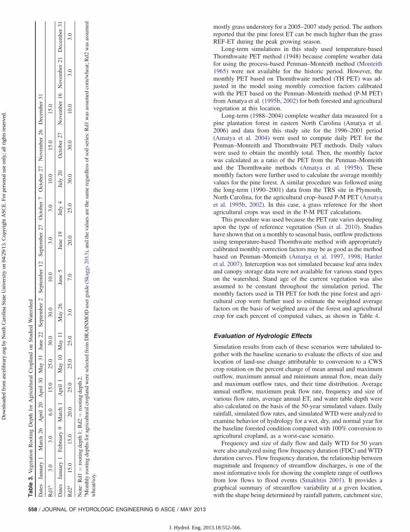
The variations of the simulated daily outflows, annual rainfall, andsimulated annual water table depth in the wettest and driest years

are compared with those of a normal year in Fig. 7. The wettest,the driest, and the normal year were selected on the basis of totalannual rainfall; seasonal patterns of rainfall for these years were notconsidered.

Year 1970 was the driest of the 50-year simulation period with a377-mm rainfall deficit [Fig. 7(a)]. The rainfall amount during thefirst half of 1970 was only 58% of that of a normal year (1994). Thesimulated water table depth on June 1 was 136 cm for baselinesimulation compared with 132 cm after conversion to a CWScrop rotation. After June 1, the simulated WTD dropped to morethan 240 cm for baseline forested fields compared with 150 cmfor agricultural cropland. This created a large soil-water deficitin both cases. As a result, the small rainfall events from May 29–December 21 did not produce predicted outflows because all therain was stored in the dry soil profile.

Interestingly, simulated water table depth on December 22 forthe baseline condition (forest) was 255 cm; the profile was so drythat the rainfall event of 24 mm on December 23 was not enough toproduce outflow. Simulated water table depth for 100% agriculturalcropland (after conversion) was closer to the surface, 157 cm, butthe 24-mm rainfall was still not enough to produce outflow onDecember 23, nor for the rest of the year [Fig. 7(a)]. Similar ob-servations were made by Amatya and Skaggs (2011) for anotherdrained pine forest in eastern North Carolina, where the water tabledropped below 250 cm. Sun et al. (2010) also found exceptionallydry soil conditions at CC and matured LP sites, with the water tabledepths retreating deeper than 1.5 m during a dry period in 2007.

The wettest year during the simulation period was 1989 (annualrainfall of 1,760 mm) with a surplus rainfall (difference betweenprecipitation and potential ET) of 476 mm. As would be expected,groundwater elevations were much higher than normal owing to theconsistent rainfall from February to August. Conversion from forestto a CWS crop rotation resulted in substantial increases in outflowsduring this wet year [Fig. 7(b)]. Not only was flow predicted duringthe winter for the CWS rotation when no flow was simulated for the

0

400

800

1,200

1,600

2,000

1950 1955 1960 1965 1970 1975 1980 1985 1990 1995 2000

Hyd

rolo

gic

co

mp

on

ents

, mm

Year

(a) (b)

Outflow Rainfall ET

0

400

800

1,200

1,600

2,000

1950 1955 1960 1965 1970 1975 1980 1985 1990 1995 2000

Hyd

rolo

gic

co

mp

on

ents

, mm

YearOutflow Rainfall ET

0

40

80

120

160

200

240

280

1950 1955 1960 1965 1970 1975 1980 1985 1990 1995 2000

Wat

er t

able

dep

th, c

m

0

40

80

120

160

200

240

280

1950 1955 1960 1965 1970 1975 1980 1985 1990 1995 2000

Wat

er t

able

dep

th, c

m

Fig. 6. Simulated water-balance components of outflow and ET with measured rainfall at the top and simulated water table depth at the bottom for(a) 100% forested area; (b) 100% agricultural cropland

562 / JOURNAL OF HYDROLOGIC ENGINEERING © ASCE / MAY 2013

J. Hydrol. Eng. 2013.18:552-566.

Dow

nloa

ded

from

asc

elib

rary

.org

by

Nor

th C

arol

ina

Stat

e U

nive

rsity

on

04/2

9/13

. Cop

yrig

ht A

SCE

. For

per

sona

l use

onl

y; a

ll ri

ghts

res

erve

d.

forest, but the peak flow rates were approximately doubled. For thebaseline simulation, only two daily flow events were more than6 mm. However, 14 peak flow rates were more than 6 mm afterconversion to CWS crop rotation [Fig. 7(b)]. The simulated maxi-mum daily outflow of 5.0 mm before conversion increased to9.8 mm after conversion.

Fig. 7 also shows the impact of the antecedent conditions. Forthe driest year (1970) [Fig. 7(a)], there was a wet antecedent (end of1969) condition that resulted in most of the winter flow. This yearwas drier than other years in terms of rainfall, but wetter than otheryears in terms of antecedent conditions. In contrast, the antecedentconditions were very dry for the wet year (1989) [Fig. 7(b)] and thenormal year (1994) [Fig. 7(c)]. As a result, there were no predictedflows in the early part of the year for either of the wettest yearsbecause of the dry antecedent conditions. The period of rewettingfrom these dry conditions is when the real differences in flow vol-umes between forest and agricultural cropland occurred. Skaggs et al.(2011) made similar observations regarding the effects of antecedentconditions on drainage flow from forest land, a wet land, and a landwith an agricultural crop for eastern North Carolina.

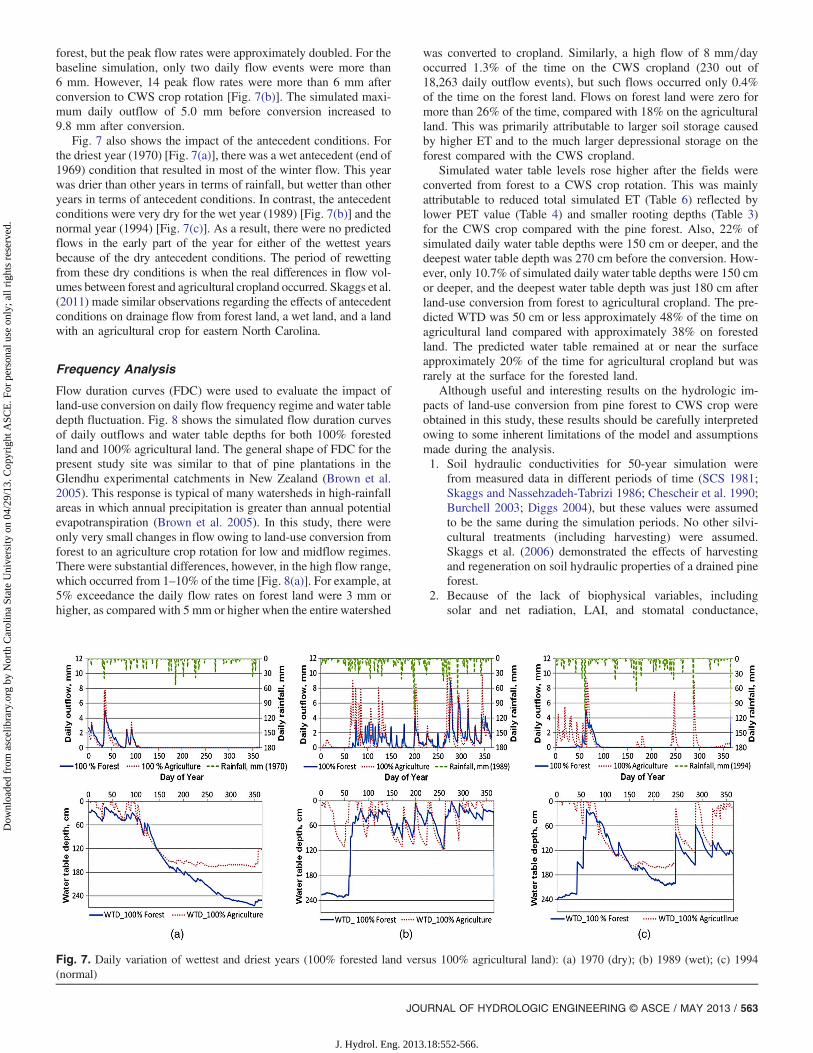
Frequency Analysis

Flow duration curves (FDC) were used to evaluate the impact ofland-use conversion on daily flow frequency regime and water tabledepth fluctuation. Fig. 8 shows the simulated flow duration curvesof daily outflows and water table depths for both 100% forestedland and 100% agricultural land. The general shape of FDC for thepresent study site was similar to that of pine plantations in theGlendhu experimental catchments in New Zealand (Brown et al.2005). This response is typical of many watersheds in high-rainfallareas in which annual precipitation is greater than annual potentialevapotranspiration (Brown et al. 2005). In this study, there wereonly very small changes in flow owing to land-use conversion fromforest to an agriculture crop rotation for low and midflow regimes.There were substantial differences, however, in the high flow range,which occurred from 1–10% of the time [Fig. 8(a)]. For example, at5% exceedance the daily flow rates on forest land were 3 mm orhigher, as compared with 5 mm or higher when the entire watershed

was converted to cropland. Similarly, a high flow of 8 mm=dayoccurred 1.3% of the time on the CWS cropland (230 out of18,263 daily outflow events), but such flows occurred only 0.4%of the time on the forest land. Flows on forest land were zero formore than 26% of the time, compared with 18% on the agriculturalland. This was primarily attributable to larger soil storage causedby higher ET and to the much larger depressional storage on theforest compared with the CWS cropland.

Simulated water table levels rose higher after the fields wereconverted from forest to a CWS crop rotation. This was mainlyattributable to reduced total simulated ET (Table 6) reflected bylower PET value (Table 4) and smaller rooting depths (Table 3)for the CWS crop compared with the pine forest. Also, 22% ofsimulated daily water table depths were 150 cm or deeper, and thedeepest water table depth was 270 cm before the conversion. How-ever, only 10.7% of simulated daily water table depths were 150 cmor deeper, and the deepest water table depth was just 180 cm afterland-use conversion from forest to agricultural cropland. The pre-dicted WTD was 50 cm or less approximately 48% of the time onagricultural land compared with approximately 38% on forestedland. The predicted water table remained at or near the surfaceapproximately 20% of the time for agricultural cropland but wasrarely at the surface for the forested land.

Although useful and interesting results on the hydrologic im-pacts of land-use conversion from pine forest to CWS crop wereobtained in this study, these results should be carefully interpretedowing to some inherent limitations of the model and assumptionsmade during the analysis.1. Soil hydraulic conductivities for 50-year simulation were

from measured data in different periods of time (SCS 1981;Skaggs and Nassehzadeh-Tabrizi 1986; Chescheir et al. 1990;Burchell 2003; Diggs 2004), but these values were assumedto be the same during the simulation periods. No other silvi-cultural treatments (including harvesting) were assumed.Skaggs et al. (2006) demonstrated the effects of harvestingand regeneration on soil hydraulic properties of a drained pineforest.

2. Because of the lack of biophysical variables, includingsolar and net radiation, LAI, and stomatal conductance,

Fig. 7. Daily variation of wettest and driest years (100% forested land versus 100% agricultural land): (a) 1970 (dry); (b) 1989 (wet); (c) 1994(normal)

JOURNAL OF HYDROLOGIC ENGINEERING © ASCE / MAY 2013 / 563

J. Hydrol. Eng. 2013.18:552-566.

Dow

nloa

ded

from

asc

elib

rary

.org

by

Nor

th C

arol

ina

Stat

e U

nive

rsity

on

04/2

9/13

. Cop

yrig

ht A

SCE

. For

per

sona

l use

onl

y; a

ll ri

ghts

res

erve

d.

process-based Penman–Monteith PET could not be usedfor the long-term simulation. Instead, the temperature-basedThornthwaite method, with correction factors developedwith short-term calibration with the Penman–Monteith PET(reflecting forest and ground vegetation), was used for estimat-ing the long-term PET used in the model.

3. The same seasonal rooting depths for 50 years were used foreach year, assuming a mature pine-forest stand. Actual rootingdepths vary with time, especially for the younger trees.

4. Canopy evaporation attributable to interception was notsimulated in this study because of the lack of LAI andcanopy-coverage data. An assumption was made that thePET estimated using the correction factors based on thePenman–Monteith method would adjust for underpredictionsof ET caused by ignoring interception. The net result may bean underestimation of ET for forested conditions.

Summary and Conclusions

This study was conducted to investigate the effect of the locationand percentage of land-use conversion on hydrological componentssuch as drainage outflow, water table depth, and evapotranspirationon the 2,950-ha drained pine forest in the lower coastal plain nearthe town of Plymouth in Washington County, North Carolina. Re-sults indicated that converting forestland to a corn–wheat–soybeanagricultural crop rotation would increase mean annual outflowsand the magnitude and frequency of high flow rates for all sizesand locations of the conversion. However, conversion of up to25% area of the 29.5 − km2 pine forest to CWS cropland was pre-dicted to have only small hydrologic effects.

The mean annual outflow was significantly different from thebaseline forest only for a 100% CWS land-use conversion. Conver-sion of up to 50% of the forest lands on the tract had substantialhydrologic effects, with increased maximum daily flow rates andfrequencies of high flow rates> 5 mmday−1. Although conversionof less than 50% in the DS location had less effect on mean annualand maximum outflows, the frequency of daily high flow rates wasconsistently higher for all land-use conversion in DS locations thanin US locations. Stednick (1996) reported as a conservative esti-mate for the Eastern Coastal Plain hydrologic region that 45%of the catchment must be harvested for a measurable increase inannual water yield. These results may have important implicationsfor land management and land-use change in terms of adverseflooding and nutrient loading effects, which have recently occurredin the southeastern Atlantic coastal plain. The effects of land-useconversion from matured pine forest to agricultural crops wereprimarily attributed to reduction in evapotranspiration. Similarresults showing reduced ET for the agricultural crops compared

with the pine forest were reported by Skaggs et al. (1991, 2011) andFernandez et al. (2007).

Downstream land-use conversion from pine forest to CWS agri-cultural crop rotation is generally thought to have a greater effect onwatershed hydrological components compared with upstream con-versions, but in this study the results were the opposite. The writersbelieve that the assumed change (on the basis of previous on-sitemeasurements) in soil-saturated hydraulic conductivity and drain-able porosity during the land-use conversion from forest to agricul-tural crops greatly influenced thewater movement and storage in thesoils. The soil types in this study were not evenly distributed acrossthe watershed; consequently, effects of the different soil types had agreater impact on the water balances than the effect of the locationof conversions. Results from additional studies in various soil andclimatic conditions may be required to further explain the effectsof soil characteristics and the locations of land-use conversions.

Acknowledgments

This work was made possible by the support of WeyerhaeuserCompany, USDA National Research Initiative (NRI, contract98-35102-6493), National Council for Stream and Air Improve-ment (NCASI), the USDA Forest Service, the Center for ForestedWetlands Research, North Carolina State University, and the PostDoctoral Course Program of National Institute of EnvironmentalResearch, Republic of Korea.

References

Amatya, D. M., Chescheir, G. M., Fernandez, G. P., Skaggs, R. W., andGilliam, J. W. (2004). “DRAINWAT-based methods for estimatingnitrogen transport in poorly drained watersheds.” Trans. ASAE, 47(3),677–687.

Amatya, D. M., Chescheir, G. M., and Skaggs, R. W. (1995a). “Hydrologiceffects of the location and size of a natural wetland in an agriculturallandscape.” Proc., Int. Conf. on Versatility of Wetlands in the Agricul-tural Landscape, American Society of Agricultural and BiologicalEngineers, St. Joseph, MI, 477–488.

Amatya, D. M., Chescheir, G. M., Skaggs, R. W., Fernandez, G. P., andBirgand, F. (1998). “Evaluation of a DRAINMOD based watershedscale model.” Proc., 7th Annual Drainage Symp.: Drainage in the21st Century, L. C. Brown, ed., American Society of Agriculturaland Biological Engineers, St. Joseph, MI, 211–219.

Amatya, D. M., Chescheir, G. M., Skaggs, R. W., and Fernandez, G. P.(2002). “Hydrology of poorly drained coastal watersheds in easternNorth Carolina.” Paper No. 022034, American Society of Agriculturaland Biological Engineers, St. Joseph, MI.

Amatya, D. M., Jha, M. K., Edwards, A. E., Williams, T. M., andHitchcock, D. R. (2011). “SWAT-based streamflow and embayment

Fig. 8. (a) Simulated daily flow frequency duration curves for watershed; (b) simulated daily water table frequency duration for field F5 for all forestand all agricultural cropland

564 / JOURNAL OF HYDROLOGIC ENGINEERING © ASCE / MAY 2013

J. Hydrol. Eng. 2013.18:552-566.

Dow

nloa

ded

from

asc

elib

rary

.org

by

Nor

th C

arol

ina

Stat

e U

nive

rsity

on

04/2

9/13

. Cop

yrig

ht A

SCE

. For

per

sona

l use

onl

y; a

ll ri

ghts

res

erve

d.

modeling of a Karst affected watershed in SC.” Trans. ASABE,54(4), 1311–1323.

Amatya, D. M., Kim, H. W., Chescheir, G. M., Skaggs, R. W., and Nettles,J. E. (2008). “Hydrologic effects of size and location of harvesting ona large drained pine forest on organic soils.” Proc., 13th Int. PeatCongress, International Peat Society, Jyväskylä, Finland, 463–467.

Amatya, D. M., and Skaggs, R. W. (2001). “Hydrologic modeling of adrained pine plantations on poorly drained soils.” Forensic Sci., 47(1),103–114.

Amatya, D. M., and Skaggs, R. W. (2011). “Long-term hydrology andwater quality of a drained pine plantation in North Carolina.” Trans.ASABE, 54(6), 2087–2098.

Amatya, D. M., Skaggs, R. W., and Gregory, J. D. (1995b). “Comparisonof methods for estimating REF-ET.” J. Irrig. Drain. Eng., 121(6),427–435.

Amatya, D. M., Skaggs, R. W., and Gregory, J. D. (1996). “Effects of con-trolled drainage on the hydrology of drained pine plantations in theNorth Carolina coastal plain.” J. Hydrol., 181(1), 211–232.

Amatya, D. M., Skaggs, R. W., and Gregory, J. D. (1997). “Evaluation of awatershed scale forest hydrologic model.” Agric. Water. Manage.,32(3), 239–258.

Amatya, D. M., and Trettin, C. C. (2007). “Annual evapotranspiration of aforested wetland watershed, SC.” Paper No. 07-2222, AmericanSociety of Agricultural and Biological Engineers, St. Joseph, MI.

Amoah, J. K. O. (2008). “A new methodology for estimating watershed-scale surface depression storage.” Ph.D. dissertation, Florida Agricul-tural and Mechanical Univ., Tallahassee, FL.

Bachmair, S., Weiler, M., and Nützmann, G. (2009). “Controls of land useand soil structure on water movement: Lessons for pollutant transferthrough the unsaturated zone.” J. Hydrol., 369(3–4), 241–252.

Brevé, M. A., Skaggs, R. W., Parsons, J. E., and Gilliam, J. W. (1997).“DRAINMOD-N, a nitrogen model for artificially drained soils.” Trans.ASAE, 40(4), 1067–1075.

Brown, A. E., Zhang, L., McMahon, T. A., Western, A. W., and Vertessy,R. A. (2005). “A review of paired catchment studies for determiningchanges in water yield resulting from alterations in vegetation.”J. Hydrol., 310(1–4), 28–61.

Burchell, M. R. (2003). “Practices to reduce nitrate-nitrogen losses fromdrained agricultural lands.” Ph.D. dissertation, North Carolina StateUniv., Raleigh, NC.

Chescheir, G. M., Amatya, D. M., Fernandez, G. P., Skaggs, R. W., andGilliam, J. W. (1998). “Monitoring and modeling the hydrology andwater quality of a lower coastal plain watershed.” Proc., Specialty Conf.on Watershed Management: Moving From Theory to Implementation,Water Environment Federation, Alexandria, VA, 215–222.

Chescheir, G. M., Amatya, D. M., Giraud, F. M., Skaggs, R. W., andGilliam, J. W. (1993). “Hydrology of a forested wetland.” Paper No.932550, American Society of Agricultural and Biological Engineers,St. Joseph, MI.

Chescheir, G. M., Amatya, D. M., and Skaggs, R. W. (1994). “Modeling thehydrology of natural forested wetlands.” Paper No. 942597, AmericanSociety of Agricultural and Biological Engineers, St. Joseph, MI.

Chescheir, G. M., Skaggs, R. W., and Gilliam, J. W. (1990). “Effects ofwater management and land use practices on the hydrology andwater quality in the Albemarle-Pamlico region.” Project No. 90-09,Albamerle-Pamlico Estuarine Study, North Carolina State Univ.,Raleigh, NC, 59.

Cho, J., Barone, V. A., and Mostaghimi, S. (2009). “Simulation of land useimpacts on groundwater levels and streamflow in a Virginia watershed.”Agric. Water Manage., 96(1), 1–11.

Dai, Z., Amatya, D. M., Sun, G., Li, C., Trettin, C. C., and Li, H. (2008).“Modeling the effect of land use change on hydrology of a forestedwatershed in coastal South Carolina.” South Carolina Water ResourcesConf., Clemson Univ. Restoration Institute, Clemson Center forWatershed Excellence, North Charleston, SC.

De Wit, M. J. M. (2001). “Nutrient fluxes at the river basin scale. I: ThePolFlow model.” Hydrol. Proc., 15(5), 743–759.

Diggs, J. A. (2004). “Simulation of nitrogen and hydrology loading offorested fields in eastern North Carolina using DRAINMOD-N II.”Master’s thesis, North Carolina State Univ., Raleigh, NC.

Fernandez, G. P., Chescheir, G. M., Skaggs, R. W., and Amatya, D. M.(2007). “Application of DRAINMOD-GIS to a lower coastal plainwatershed.” Trans. ASABE, 50(2), 439–447.

Fitzpatrick, M. L., Long, D. T., and Pijanowski, B. C. (2007). “Exploringthe effects of urban and agricultural land use on surface water chemistry,across a regional watershed using multivariate statistics.” Appl. Geo-chem., 22(8), 1825–1840.

Gassman, P. W., Reyes, M. R., Green, C. H., and Arnold, J. G. (2007). “Thesoil and water assessment tool: Historical development, applications,and future research directions.” Trans. ASABE, 50(4), 1211–1250.

Harder, S. V., Amatya, D. M., Callahan, T. J., Trettin, C. C., and Hakkila, J.(2007). “A hydrologic budget of a first-order forested watershed, coastalSouth Carolina.” J. Am. Water Resour. Assoc., 43(3), 1–13.

Kim, H. W. (2009). “Evaluation of hydrology in an agricultural watershedand nitrogen removal by constructed wetlands.” Ph.D. dissertation,North Carolina State Univ., Raleigh, NC.

Kim, H. W., Amatya, D. M., Broome, S., Hesterberg, D., and Choi, M.(2012). “Sensitivity analysis of the DRAINWAT model applied to anagricultural watershed in the lower coastal plain, North Carolina,USA.” Water Environ. J., 26(1), 130–145.

Konyha, K. D., and Skaggs, R. W. (1992). “A coupled, field hydrology.Open channel flow model: Theory.” Trans. ASAE, 35(5), 1431–1440.

Li, K. Y., Coe, M. T., Ramankutty, N., and De Jong, R. (2007). “Modelingthe hydrological impact of land-use change in West Africa.” J. Hydrol.,337(3–4), 258–268.

Li, Q., Cai, T., Yu, M., Lu, G., Xie, W., and Bai, X. (2011) “Investigationinto the impacts of land-use change on runoff generation characteristicsin the upper Huaihe River Basin, China.” J. Hydrol. Eng..

McCarthy, E. J., Flewelling, J. W., and Skaggs, R. W. (1992). “Hydrologicmodel for drained forested watershed.” J. Irrig. Drain Eng., 118(2),242–255.

Monteith, J. L. (1965). “Evaporation and environment.” Symp. of theSociety for Experimental Biology, The State and Movement of Waterin Living Organisms, G. E. Fogg, ed., Vol. 19, Academic Press,New York, 205–224.

Moriasi, D. N., Arnold, J. G., Van Leiw, M. W., Binger, R. L., Harmel,R. D., and Veith, T. L. (2007). “Model evaluation guidelines forsystematic qualification of accuracy in watershed simulations.” Trans.ASABE, 50(3), 885–900.

Nandakumar, N., and Mein, R. G. (1997). “Uncertainty in rainfall-runoffmodel simulations and the implications for predicting the hydrologiceffects of land-use change.” J. Hydrol., 192(1–4), 211–232.

Qi, S., Sun, G., Wang, Y., McNulty, S. G., and Myers, J. A. M. (2009).“Streamflow response to climate and landuse changes in a coastalwatershed in North Carolina.” Trans. ASABE, 52(3), 739–749.

SAS 9.1.3 [Computer software]. Cary, NC, SAS Institute.Shelby, J. D., Chescheir, G. M., Skaggs, R. W., and Amatya, D. M. (2005).

“Hydrologic and water quality response of forested and agriculturallands during the 1999 extreme weather conditions in eastern NorthCarolina.” Trans. ASAE, 48(6), 2179–2188.

Skaggs, R. W. (1978). “A water management model for shallow watertable soils.” Report No. 134, Water Resources Research Institute,North Carolina State Univ., Raleigh, NC.

Skaggs, R. W. (2013). “DRAINMOD users manual.” ⟨http://www.bae.ncsu.edu/soil_water/drainmod/manuals.html⟩ (Feb. 19, 2013).

Skaggs, R. W., Amatya, D. M., Chescheir, G. M., and Blanton, C. D.(2006). “Soil property changes during loblolly pine production.” PaperNo. 06-8206, American Society of Agricultural and BiologicalEngineers, St. Joseph, MI.

Skaggs, R. W., Chescheir, G. M., Fernandez, G. P., Amatya, D. M., andDiggs, J. (2011). “Effects of land use on soil properties and hydrologyof drained coastal plain watersheds.” Trans. ASABE, 54(4), 1357–1365.

Skaggs, R. W., Gilliam, J. W., and Evans, R. O. (1991). “A computer sim-ulation study of pocosin hydrology.” Wetlands, 11(1), 399–416.

Skaggs, R. W., and Nassehzadeh-Tabrizi, A. (1986). “Design drainage ratesfor estimating drain spacings in North Carolina.” Trans. ASAE, 29(6),1631–1640.

Smakhtin, V. U. (2001). “Low flow hydrology: A review.” J. Hydrol.,240(3–4), 147–186.

JOURNAL OF HYDROLOGIC ENGINEERING © ASCE / MAY 2013 / 565

J. Hydrol. Eng. 2013.18:552-566.

Dow

nloa

ded

from

asc

elib

rary

.org

by

Nor

th C

arol

ina

Stat

e U

nive

rsity

on

04/2

9/13

. Cop

yrig

ht A

SCE

. For

per

sona

l use

onl

y; a

ll ri

ghts

res

erve

d.

Soil Conservation Service (SCS). (1981). Soil Survey of WashingtonCounty, North Carolina, USDA, Washington, DC.

Stednick, J. D. (1996). “Monitoring the effects of timber harvest on annualwater yield.” J. Hydrol., 176(1–4), 79–95.

Sun, G., et al. (2010). “Energy and water balance of two contrastingloblolly pine plantations on the lower coastal plain of North Carolina,USA.” For. Ecol. Manage., 259(7), 1299–1310.

Sun, G., McNulty, S. G., Lu, J., Amatya, D. M., Liang, Y., and Kolka, R. K.(2005). “Regional annual water yield from forest lands and its responseto potential deforestation across the southeastern United States.”J. Hydrol., 308(1–4), 258–268.

Tang, Z., Engel, B. A., Pijanowski, B. C., and Lim, K. J. (2005). “Fore-casting land use change and its environmental impact at a watershedscale.” J. Environ. Manage., 76(1), 35–45.

Thanapakpawin, P., Richey, J., Thomas, D., Rodda, S., Campbell, B., andLogsdon, M. (2007). “Effects of landuse change on the hydrologic

regime of the Mae Chaem river basin, NW Thailand.” J. Hydrol.,334(1–2), 215–230.

Thornthwaite, C. W. (1948). “An approach toward a rational classificationof climate.” Geogr. Rev., 38(1), 55–94.

Tong, S. T. Y., and Chen, W. (2002). “Modeling the relationship betweenland use and surface water quality.” J. Environ. Manage., 66(4),377–393.

Weber, A., Fohrer, N., and Moller, D. (2001). “Long-term land use changesin a mesoscale watershed due to socioeconomic factors: Effects on land-scape structures and functions.” Ecol. Model., 140(1–2), 125–140.

Wilk, J., Andersson, L., and Plermkamon, V. (2001). “Hydrologicalimpacts of forest conversion to agriculture in a large river basin innortheast Thailand.” Hydrol. Proc., 15(14), 2729–2748.

Youssef, M. A., Skaggs, R. W., Chescheir, G. M., and Gilliam, J. W. (2006).“The nitrogen simulation model, DRAINMOD-N II.” Trans. ASAE,48(2), 611–626.

566 / JOURNAL OF HYDROLOGIC ENGINEERING © ASCE / MAY 2013

J. Hydrol. Eng. 2013.18:552-566.

Dow

nloa

ded

from

asc

elib

rary

.org

by

Nor

th C

arol

ina

Stat

e U

nive

rsity

on

04/2

9/13

. Cop

yrig

ht A

SCE

. For

per

sona

l use

onl

y; a

ll ri

ghts

res

erve

d.