Hydrodynamics and Heat Transfer in Two and Three ... · Reynaud, Debray, Franc, and Maitre (2005)...

Copyright © 2013 Tech Science Press FDMP, vol.9, no.2, pp.127-151, 2013

Hydrodynamics and Heat Transfer in Two andThree-dimensional Minichannels

D. Cherrared1 and E. G. Filali 1

Abstract: Our study deals with the characterization of the flow and related heattransfer in a smooth, circular minichannel. A duct with a sudden (sharp-edged) con-traction is also considered. Prediction of the pressure loss coefficient in this caseis obtained via the commercial code CFX 5.7.1. This code is based on the finitevolume method for the solution of the Navier-Stokes and offers several turbulencesmodels (in this study we use the shear stress turbulence model - SST). The nu-merical results are compared with experimental results obtained for a configurationsimilar to those considered in the numerical study. The numerical algorithm is alsovalidated by comparison with [Reynaud, Debray, Franc, and Maitre (2005); Guo,Wang, Yu, Fang, Chongfang, and Zhuo (2010)]. A good agreement is obtained withthe exception of the transition zone between laminar and turbulent regime. In thecase of duct sudden contraction, the numerical results show that the abrupt contrac-tion coefficient Kc decreases with the Reynolds number, and it is much higher thanthat of conventional tubes in laminar flow when the diameter D is less than 1mm.

Keywords: Hydrodynamics, friction factor, Heat transfer, loss coefficients, abruptcontraction, Minichannels

1 Introduction

During the last two decades, most of the studies on microchannels shows devi-ations with respect to traditional laws as unusual friction factors or shifts in thetransition between laminar and turbulent flow. It is note worthy that several stud-ies exhibit contradictory results for both mechanical and thermal characteristics ofthe flow. This is generally due to difference in the many parameters that char-acterize theses studies such as geometry (usually made of complex multichannels[Rahman (2000)]), the hydraulic diameter, the shape and surface roughness of thechannels, the fluid nature, the boundary conditions, the flow regime but specially

1 Faculty of Mechanical and Process Engineering, Houari Boumedienne University B.P. 32 El Alia,Algiers, Algeria

128 Copyright © 2013 Tech Science Press FDMP, vol.9, no.2, pp.127-151, 2013

the measurements and calculating techniques itself. For a fundamental insight intomicrofluidics, it may then be useful to reduce as much as possible the number ofparameters.

Judy, Maynes, and Web (2002) analyzed the laminar flow of water, methanol andisopropanol through circular and square sections. The results indicated that thefriction factor f for square channels with diameters of 47µm to 101µm is in goodagreement with conventional theory. In circular tubes with diameters varying from15µm to 150µm, the friction factor f showed no significant deviation of the Poiseuilleequation according to the experimental uncertainty.

Yang, Wu, Chien, and Lu (2003) studied the laminar and turbulent flows of wa-ter and a refrigerant liquid R-134a in smooth pipes with a diameter varying from0.502mm to 4.01mm. The friction factor f for the two liquids is in conformity withthe conventional equations; Poiseuille in laminar regime and Blasius in turbulentone.

Reynaud, Debray, Franc, and Maitre (2005) have realized experimental measure-ments of the friction factor and heat transfer coefficients in 2D minichannels of1.12mm to 300µm in thickness. The minimum and maximum velocities recordedon all the tests are 0.7 and 24 m/s. The friction factor is estimated from the mea-sured pressure drop along the whole channel. The heat transfer coefficient is de-termined from a local and direct measurement of both temperature and heat flux atthe wall using a specific transducer. They noted that the experimental results arein good agreement with classical correlations relative to channels of conventionalsize. The observed deviation were explained either macroscopic effects (mainly en-try and viscous dissipation effects) or imperfections of the experimental apparatus.

The application of micro-electro-mechanical systems (MEMS) have been increas-ing in many fields in recent years. Devices with dimensions of the order of micronsare developed for micro-electronic cooling systems, bipolar plates of fuel cells andcompact heat exchangers, etc. So far, a lot of researches have been conducted onmicro-flow, most of which are focused on flow characteristics in straight channelsdue to frictional resistance.

Peng, Peterson, and Wang (1994) investigated the flow characteristics of waterflowing through rectangular channel with a hydraulic diameter of 133-367µm. Itwas found that the flow friction behavior for both the laminar and turbulent flowdramatically deviated from the classical correlations. The geometric parameters,hydraulic diameter, and the aspect ratio were found to be the most important pa-rameters which had significant effects on the fluid flow through microchannels.

Liu and Grimella (2004) showed that conventional correlations offer reliable pre-dictions for the Laminar flow characteristics in the rectangular microchannels over

Hydrodynamics and Heat Transfer 129

a hydraulic diameter range of 244-974µm.

Qu and Mudawar (2002) performed experimental and numerical investigations ofpressure drop and heat transfer characteristics of single phase laminar flow in 231µmand 713µm channels. Good agreement was found between the measurements andnumerical predications, validating the use of conventional Navier-Strokes equationfor microchannels.

Adams, Abdel-Khalik, Jeter, and Qureshi (1998) investigated the single-phase forceconvection of water in circular microchannels of diameter 760µm and 1090µm.Their experimental Nusselt numbers were significantly higher than those predictedby traditional correlations. Adams, Abdel-Khalik, Jeter, and Qureshi (1999) ex-tend this work to non-circular microchannels of large hydraulic diameters, greaterthan 1130µm. All their data for the large diameters were well predicated by the[Gnielinski (1976)] correlations, leading them to suggest a hydraulic diameter ofapproximately 1200µm as the lower limit for the applicability of standard turbulentsingle-phase Nusselt correlations.

The frictional resistance in straight channels, the local resistances in expansion,contraction, divergence, convergence and elbow also influences the total pressuredrop in mini and microchannels. However, experimental studies on flow through asudden flow area contraction in micro/mini channels are still lacking in the litera-ture.

Abdelall, Hahn, and Ghiaasiaan (2005) performed several experiments to investi-gate pressure drops caused by abrupt flow area expansion and contraction in smallcircular channels. Fluids used are air and water at room temperature and near-atmospheric pressure. The diameters of larger and smaller tubes were 1.6 mmand 0.84 mm, respectively. The experimental results for water showed that ap-proximately constant expansion loss coefficients occurred for turbulent flow in thesmaller channel. The contraction loss coefficient for water was approximately 0.5while that for air in turbulent flow was a constant and matched well with theoreticalpredictions. However, the expansion loss coefficients for air were not reported.

Chalfi and Ghiaasiaan (2008) measured pressure drops caused by flow area ex-pansion and contraction under low flow conditions using air and water. The testsections consist of two capillaries with 0.84 mm and 1.6 mm diameters. The ex-perimental expansion loss coefficients obtained for air is constant and equal 0.8 forRe≥ 5000. For Re < 600, the expansion coefficients for air and water had a sharpincrease as the Reynolds number increased. The contraction loss coefficient for airin turbulent flow and water in laminar flow had a minor increase with the increaseof Reynolds number.

Yu, Li, and C. F. Ma (2006) and Li, Yu, and Ma (2007, 2008) conducted experi-


ments with nitrogen and water, and investigated single-phase and gas-liquid two-phase pressure drops caused by a sudden contraction in microtubes at room tem-perature and atmospheric pressure. The diameter of the smaller tube is 330µm. Insingle-phase flow experiments, the contraction loss coefficients for water are largerthan the experimental results from conventional tubes in the laminar flow.

Our study consists in characterizing the dynamic and thermal field of a flow insmooth, circular minichannels. Predictions of the pressure loss coefficient in sud-den contraction in the minichannels are also studied using a commercial code CFX5.7.1. This code use the finite volume method to solve the equations of Navier-Stokes and offer several turbulences models. In this study, the shear stress turbu-lence model (SST) is used. The study of thermal field is not considered in suddencontraction, we were interested to dynamic field to compare the result with ex-perimental measurements available in the literature for channels with conventionalsize.

2 Flow configuration and boundary conditions

Two configurations are considered in this study. The first configuration of the flowis a circular, smooth minichannel with a length L= 20cm and a variable diameter D.The fluid flow is coming through the entry (z= 0), with a velocity Ue. The Reynoldsnumber Re = Ue.D/v, is based on the incoming velocity Ue and the minichanneldiameter D. The selected flow conditions are taken as follow: Ue = 0.1 to 40m/sand D = 0.1 to 1mm.

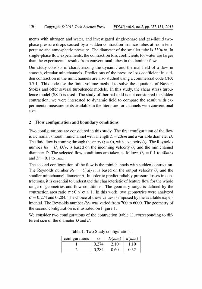
The second configuration of the flow is the minichannels with sudden contraction.The Reynolds number Red = Us.d/v, is based on the output velocity Us and thesmaller minichannel diameter d. In order to predict reliably pressure losses in con-tractions, it is essential to understand the characteristic of feature flow for the wholerange of geometries and flow conditions. The geometry range is defined by thecontraction area ratio σ : 0 ≤ σ ≤ 1. In this work, two geometries were analyzedσ = 0.274 and 0.284. The choice of these values is imposed by the available exper-imental. The Reynolds number Red was varied from 700 to 6000. The geometry ofthe second configuration is illustrated on Figure 1.

We consider two configurations of the contraction (table 1), corresponding to dif-ferent size of the diameter D and d.

Table 1: Two Study configurations

configurations σ D(mm) d(mm)

1 0,274 2,10 1,102 0,284 0,60 0,32


Figure 1: study domain (L = 5D and l = 40d)

σ represent the flow area expansion function of the ratio (A2/A1) and given as:σ = A2/A1 = (d/D)2. With A2 and A1 represents the area corresponding to thediameter D and d respectively.

In all the study, the boundary conditions include a fully developed flow at inlet,mass conservation at outlet and no-slip at the wall surface. Automatic near-walltreatment is used for turbulence model SST. Automatic near wall treatment withautomatically from wall functions to a low-Re near wall formulations as the meshis refined. One of the well known deficiencies of the k− ε model is its inabilityto handle low turbulent Reynolds number computations. Complex dumping func-tions can be added to the k− ε model, as well as the requirement of highly refinednear wall grid resolution (y+ < 0.2) in an attempt to model low turbulent Reynoldsnumbers flows. This approach often leads to numerical instability. Some of thesedifficulties may be avoided by using the k−ω model, making it more appropriatethan the k−ε model for flows requiring high near wall resolution. However, a strictlow Reynolds number implementation of the model would also require a near wallresolution of at least y+ < 2. This condition cannot be guaranteed in most appli-cations at all walls. For this reason, a new near wall treatment was developed byCFX for the k−ω based models that allows for a smooth shift from a low Reynoldsnumber form to a wall function formulation. This near wall boundary condition,named automatic near wall treatment in CFX5, is used as the default in all modelsbased on the equation (standard k−ω , SST, etc).

In this study, the fluid is incompressible and Newtonian. The regime is stationary.The fluid used is water, incoming in the channel at temperature of 20◦C and tur-bulence intensity of 5%. The following properties are used: ρ = 988.2kg/m3 and


v = 1004.10−6m2/s. To simplify the study and to reduce number elements of themesh volumes and to speed up the computation time, we opted for an axisymmetricgeometry for the first configuration.

Our calculations are compared to classical results in the laminar and turbulentregimes. For the laminar regime, it can be shown analytically that, in the caseof a fully developed flow, the Poiseuille number is constant (P0 = 24).

3 Numerical technique

The fundamental equations governing the flow phenomenon are the general equa-tion of mass, momentum and energy. The resolution of these differential equationsrequires the choice of a suitable numerical method to solve the problem. For ourcase, we choose the finite-volume method. The turbulence model used is the SSTmodel (Shear stress turbulence model) [Menter (1994)

We specially pay attention in selected grid. The mesh employed is of tetrahedralelements with prismatic refining at the wall, illustrated in figures 2 and 3.

Figure 2: Transverse section (first configuration)

Non uniform grid was generated and grid refinement close to the wall and suddencontraction zone was applied. Several successive grid refinements have been car-ried out in every case to get negligible effect of the mesh in the solutions. The meshobtained is of 1.2 million nodes and 6 million tetrahedral elements.

The CFD used is a combination of two complementary software: The Workbench9.0 processor, which makes it possible to prepare the geometry and to generate gridand the CFX solver, who solves the equations modeling the phenomenon.

The CFX solver finishes the calculations when the equation residuals calculated us-ing the specified method is below the target residual value. A convergence criterionof 10−3 is used to ensure negligibly small iteration errors (figure 4).


Figure 3: Computational geometry (second configuration)

Figure 4: convergence curves

4 Results and discussion

4.1 Flow in a smooth circular minichannels

Our simulations are of a hydrodynamic aspects and heat transfer. We looked, inparticular; the velocity profiles, boundary layer thickness, the lengths of fully de-veloped flow, the frictions factors as well as the pressure drop. Those parametersare analyzed in respect of; the effect of Reynolds number variation as well as thevariation of the diameter of the minichannels. The variation of the Nusselt numberis also studied. The obtained results are compared to the classical correlation ap-plied for the pipe with conventional size. A comparison with experimental resultsis also conducted.


4.1.1 Effect of the variation of the Reynolds number

In this part, we present the results obtained in a minichannel of diameter D = 1mm,while the length of the pipe L is 20cm. The velocity of the incoming flow variesfrom 0.1 to 40m/s.

Figures 5 and 6, shows the evolution of the velocity profiles in a section locatedat z = 10cm from the entry of the minichannel. Values of the Reynolds number,going from 5000 to 40000, in the case of a turbulent flow and between 100 to 1000for the laminar regime. It should be noted that we take care so that all the data arerecorded in a fully developed flow.

For the two regimes, we observe an increase of the maximum velocity at the centerof the minichannel, with the increase of the Reynolds number. This increase islinear as shown in figure 7.

0,0 0,4 0,8 1,2 1,6 2,0

-0,4

-0,2

0,0

0,2

0,4

Y/D

Vitesse [m/s]

Ue =0.1 m/s Ue = 0.5m/s Ue = 1 m/s

Figure 5: Velocity profiles, laminar flow

The ratio Umax/Ue is equal to 1.30 for velocities between 5 and 40m/s (turbulentflow), and 1.92 for velocities of 0.1 to 1m/s (laminar flow). For the classical pipes,the theory gives for the same ratio; the value 1.2 for the turbulent flow, and 2 forlaminar one.

The results obtained, seems to be in general agreement with those previously re-ported by the theory of the classic pipes.

The literature provides that in the case of the channel with classic size, the hydro-dynamic length of fully developed flow is function of the diameter of the pipe andthe Reynolds number for a laminar regime, and only function of the diameter of thepipe when the flow is turbulent, as mentioned:

Laminar flow: Le/D≈ 0.01.Re


0 5 10 15 20 25 30 35 40 45 50 55 60

-0,4

-0,2

0,0

0,2

0,4

Y/D

Vitesse [m/s]

Ue= 5m/s Ue=10m/s Ue=20m/s Ue=25m/s Ue=30m/s Ue=40m/s

Figure 6: Velocity profiles, turbulent flow

0,1 1 10

0,1

1

10

U m

ax [m

/s]

Ue [m/s]

Figure 7: Evolution of maximum velocity at the center of minichannel

Turbulent flow: Le/D≈ 25−40 [Schlichting and Gersten (2004)]

From our calculations, the variation in the length of fully developed flow accordingto the Reynolds number is represented figure 8, for D = 1mm. The same charactersare observed in the case of minichannels compared to the classic theory. Indeed,we observe that the length of fully developed flow increases in a linear way accord-ing to the Reynolds number for the low values. After a zone of transition locatedbetween 1000 and 5000, we observe a stabilization of the curve, meaning the inde-pendence of this length according to the Reynolds number. The calculation of theratio Le/D gives a value of 0.018 Re for laminar flow. This result is in good agree-ment with the theory of pipe with conventional size equation above. For a turbulent


0 10000 20000 30000 40000

8

12

16

20

24

28

Le [mm]

Re

Figure 8: Length of fully developed flow

0 2 4 6 8 100,0

0,1

0,2

0,3

0,4

0,5

[mm]

position Z[cm]

Ue=0.1m/s Ue=1m/s Ue=10m/s Ue=25m/s Ue=40m/s

Figure 9: Evolution of the dynamic boundary layer

flow, this ratio is equal to 25, value proposed by the classical theory [Schlichtingand Gersten (2004)].

The transition zone seems to be located between (1000 and 5000); which means,that this zone is different from that predicted for the classic pipes. This observationis also underlined by some authors [Reynaud, Debray, Franc, and Maitre (2005)].

Figure 9, represent the evolution of the hydrodynamic boundary layer through theminichannel. We can note the existence of a zone of strong velocity gradient caus-ing the formation of the boundary layer whose value seems to be stabilized whenthe flow is fully developed. The order of magnitude of this boundary layer thick-ness, varies between 0.499 and 0.43 respectively for velocity equal to 0.1 (laminar


flow) and 40m/s (turbulent flow); as maximum value. For laminar flow, the bound-ary layer invade practically all the minichannel, for turbulent one, the boundarylayer covers only one percentage of the diameter of the minichannel.

In the case of the turbulent regime, the zone of flatness decreases when the Reynoldsnumber increases, showing the inverse relation between the thickness of boundarylayer δ and the Reynolds number ( δ (z)

z = C1

R1/5ex

where; C1 ∈ [0.2,−0.3]); the tradi-

tional laws give a value of 0.37 for the constant C1.

The friction factor is estimated from the calculated pressure drop. The pressuredrop is calculated between two sections of the inlet and outlet of the minichannel.Figure 9 schematizes the variation of the friction factor according to the variationof the Reynolds number. While referring to the theoretical results of the classicpipes, the laws are:Laminar flow:

λ =64Re

= 4CF (1)

Turbulent flow:

CF =λ

4=

0.079

R1/4e

(2)

From the equilibrium of forces on a portion of fluid of length L and diameter Dsubjected to a pressure difference ∆P (assuming a hydrostatic pressure distribution),we write the relation (3) that links the parietal shear stress. We obtain the relation(4) which allows us to calculate the friction coefficient.

τp =12

ρU2mC f =

∆P.D4L

(3)

CF =∆P.D

2LρU2m

(4)

Results are reported in figure 10, which shows a good agreement between the re-sults of simulations and the formulas drawn from the classic theory.

We observe a reduction in the friction factor according to the inverse of the Reynoldsnumber for the laminar flow, and an evolution in 1/R1/4

e for the turbulent flow. Thisresult is confirmed by figure 11, the increase in the Reynolds number is accompa-nied by an increase in pressure drop according to two different rapports: laminar;67 and turbulent; 150. The order of magnitude of the pressure drop is in the allowedbeach of the values. The experiment recommends value between 15 and 20 barsfor velocity of 30m/s in the minichannel.


Figure 10: Friction factor vs Reynolds number

Figure 11: Pressure drop vs Reynolds number

4.1.2 Effect of variation of the minichannel diameter

We report figure 12, the evolution of the length of fully developed flow accordingto the diameter of the minichannel. The calculation for incoming velocity Ue =10m/s are compared to those for Ue = 25m/s. We can note that the length of fullydeveloped flow is not influenced by the change of the Reynolds number, resultalso predicted by the classical theory. The calculation of the slope of the linearcurve gives the value of 25, value observed previously by the calculations and alsoobtained by experimental results.

The curve of figure 13 gives the evolution of the average friction factor according


0,0 0,2 0,4 0,6 0,8 1,00

5

10

15

20

25

Le [mm]

Diametre D[mm]

Ue=25m/s Ue=10m/s

Figure 12: Evolution of the length of fully developed flow

Figure 13: Evolution of the friction factor vs the diameter

to the diameter of the minichannel, for incoming velocity, Ue = 25m/s. The curveshows some divergences between the numerical results and traditional laws for thepipes of classic sizes. It seems that this difference is due to the calculation of thetotal friction factor. Indeed, this coefficient is only an average of the values ofthe local friction factor over a given length. It is to note, that the length of theminichannels is not constant in all cases, to reduce computational time.

Table 2 shows the variation of the minichannel length various diameter. Thesevalues are obtained after many tests to have an optimal length of the minichannelfor calculation, but we have to be some that results are released in fully developed


flow.

Table 2: variation of the minichannel length vs diameter

D (mm) 1 0.5 0.3 0.2 0.1L (cm) 20 10 5 5 2

4.1.3 Comparison with experimental results

A comparison between our numerical results, experimental ones and traditionallaws, is made. The comparison is about the evolution of the Poiseuille number withthe Reynolds number, figure 14, for Diameter D = 1mm.

Figure 14: Poiseuille number vs Reynolds number

We can observe for Reynolds number Re < 1000 (laminar flow), that the Poiseuillenumber evolve with Reynolds number and is higher than that previous by the classiclaws. Indeed, for the laminar regime, it can be shown analytically that, in the caseof fully developed flow, the Poiseuille number is constant Po = 24. These resultsseem on the other hand close to the experimental values (Reynaud). It would seemthat the increase of the dynamic length of fully developed flow with the Reynoldsis at the origin of this phenomenon.

For Re > 5000, the Poiseuille number is of the same order of magnitude as the valuegiven by traditional laws. For the fully developed turbulent regime, and in the case


of smooth wall, the Poiseuille number can be approximated by the traditional em-pirical relation: Po = 0.079R0.75

e . The results obtained, are close to the experimentalones.

We observe that the evolution of the Poiseuille number undergoes a break of slopefor a Reynolds number ranging between 1000 and 5000. This change can be inter-preted as the transition from the laminar regime to the turbulent one.

4.1.4 Heat transfer results

In this part, we present the effect of the variation of the Reynolds number on theheat transfer in a minichannel of diameter D = 0.3mm. The length of the minichan-nel is L= 5cm. The heat flux applied to the wall of the minichannel is 100000w/m2.

Figure 15: Evolution of the temperatures

Figure 15, shows the evolution of temperature along the wall of the minichannel.We note an increase of the temperature along the mini-channel. The developmentof the thermal boundary layer, which, as well as for the dynamic one, follows ahigher evolution.

We represent, figure 16, the evolution of the thikness of dynamic and thermalboundary layer along the mini channel. The analysis of the results gives a meanvalue of the report δth/δ equal to 0.96. To note that this value is twice as big asthat given by the classic theory (δth/δu = 1/Pr1/2 = 0.4). It seems, that classicaltheory are not recommended for minichannel when the diameter is less than 1 mm.Observations already made by others authors [Reynaud, Debray, Franc, and Maitre(2005)].


Figure 16: Evolution of the thermal boundary layer

Figure 17: Nusselt number vs Reynolds number

Figure 17 represents the variation of the average Nusselt number according to theReynolds number. The increase of the Reynolds number causes the increase ofthe average Nusselt number. This means the intensification of inertial force toovercome the effect of the viscous ones. This increase of inertial force acceleratesthe movement of particles near the wall so allowing an increase of the heat transferby convection and so, a decrease of the temperature at this level.

The validation of our calculations is made by a comparison with the theoreticalvalues established for the classic channels, and experimental measurements wereobtained for a minichannel with similar dimensions to those of our study. A good


concordance is observed, with regard to the works realized in minichannels, weshall note however, that some deviations are visible with regard to the results ob-tained with classic correlations. In particular, concerning the evolution of the Nus-selt number. Indeed, the values issues from simulations, shows a light evolutionof the Nusselt number in laminaire flow, what is not the case for the classic cor-relations which predict a constant Nusselt number equal to 5.38. Concerning theturbulent flow, the orders of the Nusselt number are preserved, compared with thoseobtained by the classic theory (Nu = 0.023R0.8

e Pr1/3: Colburn equation); While ourcalculations gives 0.026 for the numerical constant.

We shall note however, that a some deviations are observed for the transition laminar-turbulent zone. This zone seems to be situated for values of Reynolds number goingfrom 1000 to 5000. These values shows that the passage between the laminar flowto the turbulent one is made in a more precise way than the classic theory denoteit. This result is also observed by numerous researchers working in the field of themini and microchannels.

4.2 Flow through minichannel with sudden contraction

Flow through channels with sudden contraction occurs in many industrial applica-tions. The flow separation in the vicinity of the contraction plane causes an increasein pressure loss, which affects erosion rates and heat and mass transfer at the sepa-ration and reattachment regions.

Figure 18: Schematic of the flow through a pipe with a sudden contraction

In this part the values of Reynolds numbers considered are between 700 and 6000.


a) (D=0.6mm, d=0.32mm, =0.284)

b) (D=2,10mm, d=1,10mm, =0.274)

Figure 19: Contraction loss coefficient Kc (Laminar flow)

The CFD predictions of the pressure loss coefficient for this geometry and flowconfigurations are compared with the measurements for laminar and turbulent flowof Guo, Wang, Yu, Fang, Chongfang, and Zhuo (2010).

The pressure loss through the contraction is caused by two consecutive processes:(1) contraction of the flow to the vena contracta, and (2) expansion to the wall ofthe small pipe (figure 18). The latter is an “uncontrolled” expansion against anadverse pressure gradient. In order to determine the overall pumping power in apiping system (minichannel), it is essential to have reliable design procedures to


predict pressure losses. It is also important to know the flow details of the separa-tions upstream and downstream of the contraction plane to avoid placing sensitiveequipment in these regions (figure 18)

The pressure loss coefficient for a sudden contraction is defined as

Kc =∆Pt12

1/2ρU22

(5)

Where ∆Pt12 is the total pressure drop due to the contraction, and 1/2ρU22 is the

kinetic pressure at Station 2. ∆Pt12 is defined as the total pressure drop betweenStation 1 in the large pipe and Station 2 in the small pipe. Station 1 and 2 arelocated in the fully developed regions upstream and downstream of the contractionrespectively, outside the region of influence of the contraction.

When a fluid flows through a sudden contraction, the mechanical energy loss takesplace predominantly during the deceleration following the vena-contracta.

The variation of the sudden contraction loss coefficients in laminar region areshown in Figure 19. In the laminar flow region, the numerical results indicate thatKc decreases with Red increasing and it is much higher than that of conventionaltubes [Idel’cik (1986)].

When the diameter increases, Kc decreases and the difference between the experi-ment results and Idel’cik’s results becomes smaller. There is a good agreement be-tween the experimental and numerical results (CFX) in mini-channels. Accordingto the equation of contraction loss coefficient (eq. 5), we can explain the decrease ofKc by the important increase of velocity compared to that of the pressure difference∆P.

The sudden contraction loss coefficients for turbulent regime are shown in Fig-ure 20. The numerical results indicate that Kc increases to a maximum value andthen it decreases slightly with Red increasing. The curve of Kc shows a smallergap with that of the conventional tube. When the diameter increases, the Kc fromthe numerical data does not change while Red increasing. There is enough goodagreement between the experimental and numerical results (CFX) in minichannel.

The CFD predictions of the upstream and downstream separation regions for 700≤Red ≤ 6000 are shown in figures 21 and 22. Predictions using CFX code displaysimilar trends. These trends show an increase of the separation length and height.The variation of the separation length is greater than the height variation. However,in turbulent flow, the separation length downstream of contraction decreases whileRed increasing. This can be due to the appearance of a small vortex at the corner ofthe contraction, which can also affect the size of the downstream separation length.


a) (D=0.6mm, d=0.32mm, =0.284)

b) (D=2,10mm, d=1,10mm, =0.274)

Figure 20: Contraction loss coefficient Kc (Turbulent flow)

5 Conclusion

Simulations are made with the commercial code CFX5.7.1were conducted in minichan-nels. Dynamics aspect and heat transfer are analyzed on one size diameter ofminichannel. Effect of the local resistance of flow across sudden contraction isalso studied. In the results obtained are rich in information for the dynamic aspectsand heat transfer the parameters are Reynolds number, diameter of the minichannel,Poiseuille number, boundary layer and Nusselt number. In addition to the results


a) upstream

b) downstream

Figure 21: Separation length Lx and height Lr predicted by CFX at different Red

(Laminar flow, D=0.6mm, d=0.32mm, σ=0.284)

from the theory, established for the traditional pipes, we have experimental resultsobtained for a minichannel of size similar to those of our study. The validationof our calculations is thus made by a comparison with experimental measurements[Reynaud, Debray, Franc, and Maitre (2005)] and theoretical values. A good agree-ment is observed, note however that as light deviation is observed concerning thetransition zone between laminar and turbulent regime. This zone seems to be lo-cated for values of Reynolds number going from 1000 and 5000. This result wasconfirmed by many researchers working in the field of the mini and microfluidics.These values show that the transition zone is more precisely pointed than the clas-sical theory predicted it. The results of this study are not likely to give in cause


a) upstream

b) downstream

Figure 22: Separation length Lx and height Lr predicted by CFX at different Red

(Turbulent flow, D=0.6mm, d=0.32mm, σ=0.284)

validity of the traditional laws in the case of the mini-channels until a diameterof 0.1mm. We showed that deviations are observed compared to the traditionalcorrelations, but generally, a good agreement is noted.

Concerning the sudden contraction, in the laminar flow region, the contraction co-efficient Kc decreases with Red increasing. The Kc from the numerical result ofminichannel decreases as the diameter increases. When the diameter increases, thedifference in Kc between the numerical results on minichannel and the correlationwith conventional tubes becomes smaller. The numerical study showed that the re-sults of pressure loss coefficient are almost superposed with the experimental ones


[Guo, Wang, Yu, Fang, Chongfang, and Zhuo (2010)].

Acknowledgement: The authors would like to acknowledge the support pro-vided by the United Arab Emirates University. This work was financially supportedby the Research Affairs at the university under a contract no. 01-05-7-11/09.

References

Abdelall, F. F.; Hahn, G.; Ghiaasiaan, S. M. (2005): Pressure drop causedby abrupt flow area changes in small channels. Experimental Thermal and FluidScience, vol. 29, no. 4, pp. 425–434.

Adams, T. M.; Abdel-Khalik, S. I.; Jeter, S. M.; Qureshi, Z. H. (1998): An ex-perimental investigation of single-phase forced convection in microchannels. Int.J Heat Mass Transfer, vol. 41, no. 6-7, pp. 851–857.

Adams, T. M.; Abdel-Khalik, S. I.; Jeter, S. M.; Qureshi, Z. H. (1999): Ap-plicability of traditional turbulent single-phase forced convection correlations tonon-circular microchannels. Int.J Heat Mass Transfer, vol. 42, no. 23, pp. 4411–4415.

Chalfi, T. Y.; Ghiaasiaan, S. M. (2008): Pressure drop caused by flow areachanges in capillaries under low flow conditions. International Journal of Multi-phase Flow, vol. 34, no. 1, pp. 2–12.

Gnielinski, V. (1976): New equations for heat and mass transfer in turbulent pipeand channel flow. Int. Chem. Eng., vol. 16, no. 2, pp. 359–368.

Guo, H.; Wang, L.; Yu, J.; Fang, Y. E.; Chongfang, M. A.; Zhuo, L. I. (2010):Local resistance of fluid flow across sudden contraction in small channels. Front.Energy Power Eng. China, vol. 4, no. 2, pp. 149–154.

Idel’cik, I. E. (1986): Handbook of Hydraulic Resistance. Hemisphere Publish-ing Corporation, New York, 2nd edition.

Judy, J.; Maynes, D.; Web, B. W. (2002): Characterisation of frictional pressuredrop for liquid flows through microchannels. International Journal of Heat andMass Transfer, vol. 45, no. 17, pp. 3477–3489.

Li, Z.; Yu, J.; Ma, C. F. (2007): Local resistances of single-phase flow acrossabrupt expansion and contraction in small channels. Journal of Chemical Industryand Engineering, vol. 58, no. 5, pp. 1127–1131.

Li, Z.; Yu, J.; Ma, C. F. (2008): Characteristics of pressure drop for single-phaseand two-phase flow across sudden contraction in micro tubes. Science in ChinaSeries E, vol. 51, no. 2, pp. 162–169.


Liu, D.; Grimella, S. V. (2004): Investigation of liquid flow in microchannels.AIAA J.Thermophys. Heat Transfer, vol. 18, pp. 65–72.

Menter, F. R. (1994): Two-equation eddy-viscosity turbulence models for engi-neering applications. AIAA Journal, vol. 32, no. 8, pp. 1598–1605.

Peng, X. F.; Peterson, G. P.; Wang, B. X. (1994): Frictional flow characteristicsof water flowing through rectangular microchannels. Experimental Heat Transfer,vol. 7, no. 4, pp. 249–264.

Qu, W.; Mudawar, I. (2002): Experimental and numerical study of pressuredrop and heat transfer in a single-phase microchannel heat sink. Int.J. Heat MassTransfer, vol. 45, pp. 2549–2565.

Rahman, M. M. (2000): Measurements of heat transfer in microchannel heatsinks. International Commun. Heat Mass Transfer, vol. 27, no. 4, pp. 495–506.

Reynaud, S.; Debray, F.; Franc, J. P.; Maitre, T. (2005): Hydrodynamics andheat transfer in two-dimensional minichannels. International Journal of Heat andMass Transfer, vol. 48, no. 15, pp. 3197–3211.

Schlichting, H.; Gersten, K. (2004): Boundary layer theory. Springer, 8threvised and enlarged revision edition.

Yang, C. Y.; Wu, J. C.; Chien, H. T.; Lu, S. R. (2003): Friction characteristicsof water, r-134a, and air in small tubes. Microscale Thermophys. Eng., vol. 7, no.4, pp. 335–348.

Yu, J.; Li, Z.; C. F. Ma, C. F. (2006): Experimental study of pressure loss dueto abrupt expansion and contraction in mini-channels. In Proceedings of the 13thInternational Heat Transfer Conference, Sydney. Begell House.

Appendix A: Nomenclature

D Diameter of the channel, mm

L Length of the channel, mm

Le Length of establishment, mm

U Velocity, m/s

CF Average friction factor

d Small tube diameter, mm

Kc Pressure loss coefficient


l Small tube length, mm

Lx1 Upstream separation length, µm

Lr1 Upstream separation height, µm

Lx2 Downstream separation length, µm

Lr2 Downstream separation height, µm

A Flow area, mm2

Greek Symbols

µ Dynamic viscosity, Pa.s

ρ Mass density, kg/m2

v Kinematic viscosity, m2/s

δ Thickness of the dynamic boundary layer, mm

δτη Thickness of the thermal boundary layer, mm

Non-dimensional Numbers

Re Reynolds number

Nu Nusselt number

Po Poiseuille number,[CF ,Re]

Pr Prandtl number

y+ Non dimensional wall distance

Hydrodynamics and Heat Transfer in Two and Three ... · Reynaud, Debray, Franc, and Maitre (2005)...

Documents

Transcript of Hydrodynamics and Heat Transfer in Two and Three ... · Reynaud, Debray, Franc, and Maitre (2005)...