Hydrodynamic Modeling of the

Mundaú-Manguaba Estuarine-

Lagoon System, Brazil

____________________________________________________

Linnea Larsson

Staffan Nilsson

Examensarbete

TVVR 14/5006

Division of Water Resources Engineering

Department of Building and Environmental Technology

Lund University

Hydrodynamic Modeling of the Mundaú-

Manguaba Estuarine-Lagoon System, Brazil

Linnea Larsson

Staffan Nilsson

Cover: Finite element mesh of Mundaú-Manguaba Estaurine-Lagoon

System created with modeling software.

Pictures without references are property of the authors and figures without

references are created in the modeling software.

Avd för Teknisk Vattenresurslära

TVVR-14/5006

ISSN 1101-9824

Abstract Title: Hydrodynamic Modeling of the Mundaú-Manguaba Estuarine-

Lagoon System, Brazil

Authors: Linnea Larsson and Staffan Nilsson

Supervisors: Professor Carlos Ruberto Fragoso Jr., Center of Technology,

Federal University of Alagoas, Brazil

Professor Magnus Larson, Department of Water Resources

Engineering, Lund University, Sweden

Background: Lagoons are shallow coastal water bodies which occupy 13 % of

the world’s total coastlines. Healthy lagoons have a rich aquatic

fauna and can provide an economic benefit for the people living

in its vicinity. Due to anthropogenic activities, the water quality in

many lagoons is deteriorating. The Mundaú-Manguaba Estuarine-

Lagoon System is no exception. BOD-rich water from the nearby

sugar plantations along with large amount of untreated sewage

from the nearby city of Maceió are contributing to the

deteriorating water quality in the lagoon system. A computerized

model can be a useful tool in terms of forecasting the effects of

different actions taken to improve the water quality. Such a

model already exists, called IPH-ECO, but uses data collected in

1984 and consequently needs a thorough overhaul. The

morphology of the lagoon system has changed mainly due to

sediment infilling; therefore the model needs to be updated

regarding bathymetry and sediments.

Objectives: The purpose of this master thesis is to construct an updated

hydrodynamic model over the Mundaú-Manguaba Estuarine-

Lagoon System in Brazil. In order to achieve this, bathymetry and

sediment information needs to be collected, analyzed and finally

digitized. A field camping will be executed where data regarding

depth and salinity variation in the lagoons will be collected. Two

scenarios will be tested with the newly calibrated model to

demonstrate the usability of the model.

Procedure: This thesis was initiated in September 2013 with a literature

review where lagoons in general and the Mundaú-

Manguaba Estuarine-Lagoon System in particular were studied.

Data collection and field measurements were carried out in

Maceió, Brazil, between January and March 2014. During this

time a new field campaign was carried out in order to get updated

data concerning depth and salinity.

To run the IPH-ECO model the boundary conditions had to be

updated. That includes tidal fluctuations, river flows, bathymetry

and Chezy coefficients.

With the data collected from the sensors various new simulations

were performed in IPH-ECO in order to calibrate the model. When

the calibration process was completed the correlation between

model and sensor was evaluated. Lastly the scenarios were

simulated.

Conclusions: Mundaú lagoon could be calibrated well hydrodynamically with

high correlation between sensor data and model. The calibration

of Manguaba lagoon did not provide as satisfying results due to

the lack of data concerning bathymetry and sediments.

The two different scenarios were simulated successfully and show

that the model can be used to predict future flooding in case of

an extreme wet season and improve the water quality by the

decreased renewal time which a new ocean inlet would bring.

It is recommended that a new bathymetry survey is conducted in

the southern part of Manguaba so that the whole lagoon system

can be calibrated hydrodynamically. It is also recommended that

calibration continues regarding lagoon salinity.

Keywords: MMELS, CELMM, IPH-ECO, Mundaú lagoon, Manguaba lagoon,

choked lagoon, Maceió, hydrodynamic modeling, water quality

forecasting, Aqua troll 200, bathymetry, water exchange

Preface This master thesis on Hydrodynamic Modeling of the Mundaú-

Manguaba Estuarine-Lagoon System, Brazil was carried out in Maceió, Brazil in

cooperation with Federal University of Alagoas and completed at Faculty of

Engineering, Lund University. It was conducted during the time period January to

June in 2014.

We would like to give our deepest regard to our supervisor in Brazil Carlos Ruberto

Fragoso Jr.. During our stay in Brazil he provided specialist knowledge regarding the

computer software and gave useful insight regarding our calibration process.

Despite his workload, he always gave the project his full commitment. Our deepest

appreciation is also given to our supervisor in Sweden Magnus Larson, who helped

us realizing this MFS-project and came with valuable insight and support during the

completion of our thesis.

Our deepest gratitude also goes out to the master students at Universidade Federal

de Alagoas, who helped in the process of gathering information from websites

which were normally written in Portuguese. Among these students, two of them

deserve a special mention; Denis Duda and Almir Nunes. They gave their hearts and

souls in order to make our stay in Brazil the best one possible. We are proud to call

them our friends.

Linnea and Staffan Lund, 2014

Glossary ANA Agência Nacional de Águas

Anthropogenic Having its origin in the influence of human activity

on nature

Bathymetry Underwater equivalent to topography

BOD Biochemical Oxygen Demand is a measurement of how

much oxygen is required for aerobic biological organisms

in a body of water to break down biological material

CELMM Complexo Estaurino Lagunar Mundaú-Manguaba

Chezy A friction coefficient which describes the energy loss.

Consolidation A geological process whereby a soil decreases in volume

Diagenesis The process of chemical and physical change in deposited

sediment during its conversion to rock.

Eustatic sea level rise Relating to worldwide changes in sea level, caused by the

melting of ice sheets, movements of the ocean floor,

sedimentation, etc

Littoral drift The longshore sediment transport along the beach line

MMELS Mundaú-Manguaba-Estaurine-Lagoon System (English

equivalent to CELMM)

Morphology The study of shape and changes in the landscape related

to sediment erosion and deposition

Tidal prism The total amount of water flowing into or out of an inlet

with the rise and fall of the tide, excluding any freshwater

discharges

Tidal range The difference in height between successive high and low

tides

UFAL Universidade Federal de Alagoas

Table of Contents

1 Introduction .................................................................................................... 1

1.1 Background ............................................................................................. 1

1.2 Objectives ............................................................................................... 2

1.3 Procedure ................................................................................................ 2

2 Coastal Lagoons and Their Physical Properties................................................. 5

2.1 General Characteristics ............................................................................ 5

2.2 Classification of Lagoons .......................................................................... 5

2.3 Water Exchange ...................................................................................... 6

2.4 Sediment Transport ............................................................................... 12

2.5 Water Quality Aspects ........................................................................... 12

3 Mundaú-Manguaba Estuarine-Lagoon System .............................................. 15

3.1 Overview ............................................................................................... 15

3.2 Climatology ........................................................................................... 16

3.3 Hydrographic Conditions and Morphology ............................................. 18

3.4 Water Exchange .................................................................................... 20

3.5 Sediment Transport and Morphological Change .................................... 22

3.6 Water Quality ........................................................................................ 23

4 Field Measurements...................................................................................... 25

4.1 Previous Studies .................................................................................... 25

4.2 Experimental Setup and Procedure ........................................................ 25

4.3 Data Collected ....................................................................................... 27

5 The IPH-ECO Model ....................................................................................... 29

5.1 Basic Theory .......................................................................................... 29

5.2 Numerical Formulation .......................................................................... 30

5.3 Model Input and Setup .......................................................................... 31

5.4 Calibration Process ................................................................................ 35

6 Results .......................................................................................................... 41

6.1 Calibration Results ................................................................................. 41

6.2 Scenarios ............................................................................................... 43

6.3 Renewal Time ........................................................................................ 45

6.4 Vector Fields .......................................................................................... 46

7 Discussion ..................................................................................................... 51

7.1 Calibration ............................................................................................. 51

7.2 Estimation of Correlation ....................................................................... 52

7.3 Renewal Time ........................................................................................ 52

7.4 Scenarios ............................................................................................... 53

7.5 Future Recommendations ..................................................................... 54

7.6 Sources of Error ..................................................................................... 55

8 Conclusions ................................................................................................... 57

Bibliography.......................................................................................................... 59

Appendix I ............................................................................................................ 63

Appendix II............................................................................................................ 65

Appendix III........................................................................................................... 69

Appendix IV .......................................................................................................... 71

1

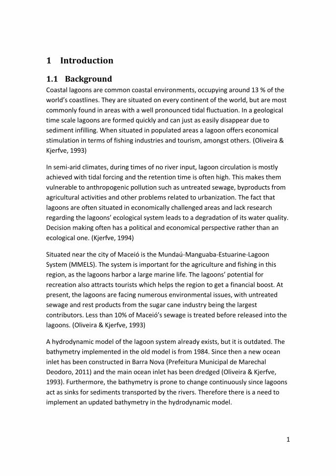
1 Introduction

1.1 Background Coastal lagoons are common coastal environments, occupying around 13 % of the

world’s coastlines. They are situated on every continent of the world, but are most

commonly found in areas with a well pronounced tidal fluctuation. In a geological

time scale lagoons are formed quickly and can just as easily disappear due to

sediment infilling. When situated in populated areas a lagoon offers economical

stimulation in terms of fishing industries and tourism, amongst others. (Oliveira &

Kjerfve, 1993)

In semi-arid climates, during times of no river input, lagoon circulation is mostly

achieved with tidal forcing and the retention time is often high. This makes them

vulnerable to anthropogenic pollution such as untreated sewage, byproducts from

agricultural activities and other problems related to urbanization. The fact that

lagoons are often situated in economically challenged areas and lack research

regarding the lagoons’ ecological system leads to a degradation of its water quality.

Decision making often has a political and economical perspective rather than an

ecological one. (Kjerfve, 1994)

Situated near the city of Maceió is the Mundaú-Manguaba-Estuarine-Lagoon

System (MMELS). The system is important for the agriculture and fishing in this

region, as the lagoons harbor a large marine life. The lagoons’ potential for

recreation also attracts tourists which helps the region to get a financial boost. At

present, the lagoons are facing numerous environmental issues, with untreated

sewage and rest products from the sugar cane industry being the largest

contributors. Less than 10% of Maceió’s sewage is treated before released into the

lagoons. (Oliveira & Kjerfve, 1993)

A hydrodynamic model of the lagoon system already exists, but it is outdated. The

bathymetry implemented in the old model is from 1984. Since then a new ocean

inlet has been constructed in Barra Nova (Prefeitura Municipal de Marechal

Deodoro, 2011) and the main ocean inlet has been dredged (Oliveira & Kjerfve,

1993). Furthermore, the bathymetry is prone to change continuously since lagoons

act as sinks for sediments transported by the rivers. Therefore there is a need to

implement an updated bathymetry in the hydrodynamic model.

2

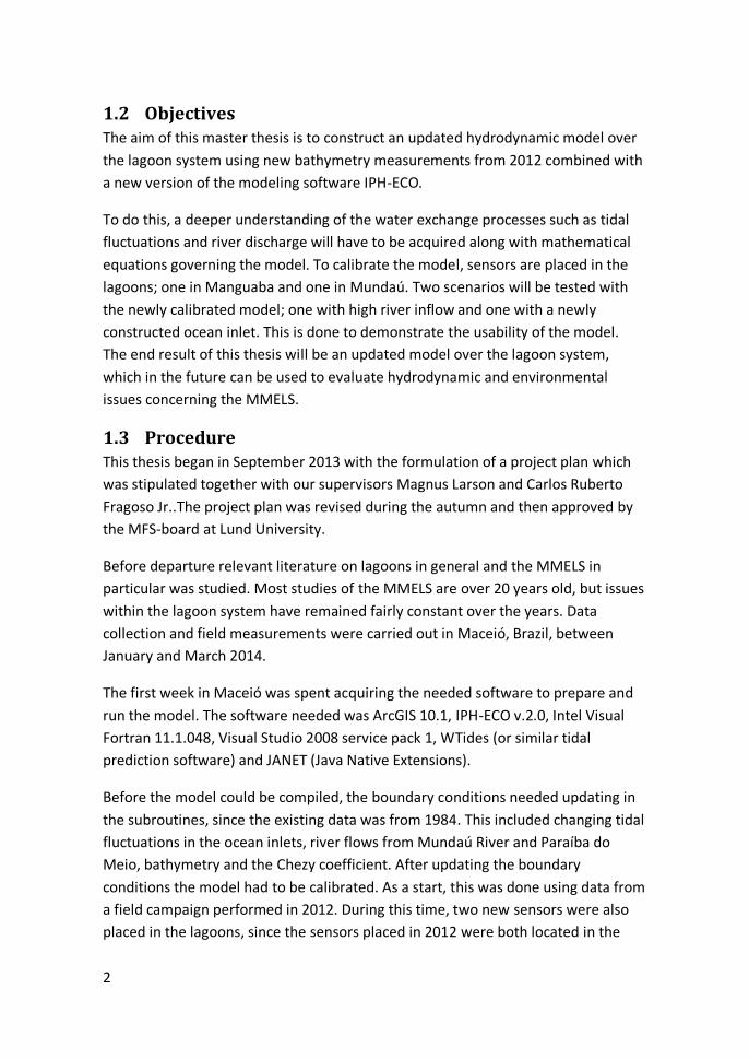
1.2 Objectives The aim of this master thesis is to construct an updated hydrodynamic model over

the lagoon system using new bathymetry measurements from 2012 combined with

a new version of the modeling software IPH-ECO.

To do this, a deeper understanding of the water exchange processes such as tidal

fluctuations and river discharge will have to be acquired along with mathematical

equations governing the model. To calibrate the model, sensors are placed in the

lagoons; one in Manguaba and one in Mundaú. Two scenarios will be tested with

the newly calibrated model; one with high river inflow and one with a newly

constructed ocean inlet. This is done to demonstrate the usability of the model.

The end result of this thesis will be an updated model over the lagoon system,

which in the future can be used to evaluate hydrodynamic and environmental

issues concerning the MMELS.

1.3 Procedure This thesis began in September 2013 with the formulation of a project plan which

was stipulated together with our supervisors Magnus Larson and Carlos Ruberto

Fragoso Jr..The project plan was revised during the autumn and then approved by

the MFS-board at Lund University.

Before departure relevant literature on lagoons in general and the MMELS in

particular was studied. Most studies of the MMELS are over 20 years old, but issues

within the lagoon system have remained fairly constant over the years. Data

collection and field measurements were carried out in Maceió, Brazil, between

January and March 2014.

The first week in Maceió was spent acquiring the needed software to prepare and

run the model. The software needed was ArcGIS 10.1, IPH-ECO v.2.0, Intel Visual

Fortran 11.1.048, Visual Studio 2008 service pack 1, WTides (or similar tidal

prediction software) and JANET (Java Native Extensions).

Before the model could be compiled, the boundary conditions needed updating in

the subroutines, since the existing data was from 1984. This included changing tidal

fluctuations in the ocean inlets, river flows from Mundaú River and Paraíba do

Meio, bathymetry and the Chezy coefficient. After updating the boundary

conditions the model had to be calibrated. As a start, this was done using data from

a field campaign performed in 2012. During this time, two new sensors were also

placed in the lagoons, since the sensors placed in 2012 were both located in the

3

mangrove channels near the ocean inlet. The new sensors were placed far from

each other, one in the middle of each lagoon. The sensors measured water level,

temperature and actual conductivity.

With the data collected from the sensors various new simulations were performed

in IPH-ECO in order to calibrate the model. This was done in Lund between March

and May 2014. After finishing the calibration process the correlation between the

model and the sensors was calculated using different statistical factors in order to

determine how well they match. The renewal time was calculated using both IPH-

ECO and the sensor readings. Thereafter two different scenarios were simulated;

one for a rather extreme wet season and one with an extra ocean inlet. Lastly,

vector fields were plotted to get a visual representation of the different scenarios.

4

5

2 Coastal Lagoons and Their Physical Properties

2.1 General Characteristics According to Kjerfve (1994) a lagoon can be defined as “a shallow coastal water

body separated from the ocean by a barrier, connected at least intermittently to

the ocean by one or more restricted inlets, and usually orientated shore-parallel”.

Lagoons were formed 15,000 years ago during the eustatic sea level rise which

caused water to flood low lying coastal areas and river valleys. Due to coastal

processes barriers have since been formed between the ocean and the lagoons. In

a geological time scale lagoons have a short life span, were formed very recently

and can disappear rapidly due to sediment infilling. (Kjerfve & Magill, 1989)

Coastal lagoons can be found on all continents in the world but tend to be less

common in Europe. Despite problems concerning water quality in lagoons,

scientific studies are rarely conducted. Water management issues in these areas

are handled with political and economical benefits in mind, rather than decisions

based on scientific studies. (Oliveira & Kjerfve, 1993)

2.2 Classification of Lagoons Lagoons can be characterized into choked,

restricted or leaky depending on how they

are connected to the ocean.

Choked lagoons are often classified as

lagoons with only one inlet, with a cross-

sectional area much smaller than the

lagoon’s area. They are often found along

coast lines with medium to high wave

energy where the tidal range is low and they

are often situated shore-normal. The narrow

inlet functions as a tidal dampening filter,

reducing the amplitude with up to 99%. As a

consequence of this, the tidal prism is

smaller in this type of lagoon than in other

types. If the small tidal prism is combined

with low freshwater input and high

evaporation (which is the case in an arid

climate) the lagoons can become hyper

Figure 1. Principal sketch over the different types of lagoons (Kjerfve, 1994).

6

saline. If the coastal area nearby the inlet experiences a high littoral drift the inlet

can be closed off and the lagoon can turn in to a salt flat. Wind forces govern the

internal mixing of the lagoon, and since depth rarely exceeds a few meters, they

tend to be vertically homogenous. The retention time of a chocked lagoon is often

quantified in months or years. (Kjerfve, 1994)

Restricted lagoons have two or more openings to the ocean and present a higher

degree of tidal mixing than choked lagoons. They are found in areas with low tidal

range and low to medium wave energy. The lower wave energy translates into

smaller littoral drift explaining the fewer barriers to the ocean. Salinity is more

stable and governed by fresh water runoff from contributing rivers. A greater tidal

mixing also means a lower retention time compared to chocked lagoons. (Kjerfve,

1994)

Leaky lagoons are shore-parallel with unrestricted openings towards the ocean.

They are found in areas were the tidal forces are sufficiently strong to counteract

any littoral drift from closing off the openings. Most leaky lagoons present an

oceanic salinity, but they can also have salinities similar to estuaries. (Kjerfve, 1994)

2.3 Water Exchange

2.3.1 Tides

Tides are produced by many different factors, out of which the gravitational and

centrifugal forces between the earth, the moon and the sun are the most

important. The moon provides the strongest influence. The moon and the earth are

held in position relative to one another by two forces; gravitational forces that

attract the two masses and centrifugal forces that keep them apart. The centrifugal

forces are equal in direction and magnitude on earth, while the gravitational forces

are much stronger on the side facing the moon. Thus, the net effect of these two

forces depends on the location on the earth relative the position of the moon.

(Ricketts, et al., 1985)

The sun also generates tidal forces, but only about half as much as the moon

because of its great distance to the earth. However, when the moon and the sun

are in a line with the earth during a new moon or a full moon their forces are

combined, meaning that tidal forces of greater range are created; these are known

as spring tides. The opposite, called neap tides, occurs when the moon and the sun

are at right angles to one another. Then the tidal forces of the sun partially cancel

out those of the moon resulting in tides of minimum range. (Ricketts, et al., 1985)

7

The combination of solar and lunar influences mentioned above is sufficient to

explain the fairly even progression of low and high tides. Semi-diurnal tides, which

are common along the Atlantic coastline, consist of two tidal cycles per lunar day. A

lunar day takes 24 hours and 50 minutes to finish. There is also something called

mixed semi-diurnal tides which are characterized by pairs of high tides and pairs of

low tides that vary greatly in magnitude. Their varying magnitude can be related to

the declination of the moon. (Ricketts, et al., 1985) A diurnal tidal cycle is

distinguished by one high and one low tide in one lunar day. (NOAA, 2008)

Apart from the influences from the moon and the sun, there are over 360 active

tidal components with periods ranging from eight hours to 18.6 years. The ones

mentioned in the table below stands for 83% of the total tide generating force.

(Gosh, 1998)

Figure 2. Major tidal components (Gosh, 1998).

The character of a tide can be determined by the following ratio:

,

where the symbols stand for the amplitude of the tidal components. If the ratio is

less than 0.25 the tide is semi-diurnal. When the ratio is between 0.25 and 1.5 the

tide is considered mixed but predominantly semi-diurnal. The tide is characterized

as mixed but predominantly diurnal if the ratio is between 1.5 and 3.0. If the ratio

is greater than 3.0 the tide is diurnal. (Gosh, 1998)

Tides are dependent on local conditions and as a consequence they vary

substantially around the world. Tides are altered to a large extent near coasts and

8

estuaries due to local effects. These local effects are however difficult to calculate

from tide-generating forces. Instead, it is convenient to perform a harmonic

analysis based on tidal records in order to predict tides. The tidal records are split

up into different components, which have the same periods as the harmonic

components. By assuming that the components from the tidal records will vary

with time in the same way as the corresponding harmonic components, it is

possible to make tide predictions. When performing a harmonic analysis, a long

record of tidal curves is essential due to the complex nature of tide curves. At least

one year is required, but ideally a 19 year long record exists. This type of harmonic

analysis is generally available for all harbors. (Gosh, 1998)

2.3.2 Lagoon Mixing

Mixing in a lagoon depends on numerous factors such as geometry of the lagoon

and the inlet channels, tidal amplitude, wind speed and wind direction relative to

the lagoon orientation, evaporation, and gravitational mixing due to temperature

and salinity differences inside the lagoon (Miller, et al., 1990).

Differences in salinity and temperature forces the denser water towards the

bottom, and can lead to vertical stratification in a water body. However, since

lagoons typically are shallow, wind driven currents circulate the water making it

vertically homogenous. A horizontal stratification is more commonly found in

lagoons, and this also contributes to the lagoon’s circulation. Vertical stratification

can however develop in a lagoon during times of very low river inflow. (Kjerfve &

Magill, 1989)

Mixing by wind stress is a result of the water being displaced in the downwind

direction, causing a set-up in the downwind direction and a set-down in the upwind

direction. The height difference between the set-up and the set-down, or the

gradient, can be estimated by τ/ρgH, where H is the depth in the lagoon, τ is the

wind shear stress and ρg expresses the weight of the water. (Miller, et al., 1990)

The wind driven mixing is more pronounced when the wind direction is parallel to

the long side of the lagoon. As Figure 3 shows, wind is driving water near the

surface downwind, while the return flow is along the bottom of the lagoon. (Miller,

et al., 1990)

9

Figure 3. Principal sketch over wind forced tidal mixing (Kjerfve & Magill, 1989).

2.3.3 Water Balance

A water balance is the sum of all terms adding or removing water from a given

control volume. The equation is a continuum which means that the difference

between positive and negative terms in the equation is represented by a change in

volume. For a lagoon the water balance can be written as:

where dV/dt denotes the long-term change of the control volume, P is the

precipitation, E is the evaporation, D is the fresh water inflow from rivers and from

surface runoff and G is the ground water seepage. A is an advective term which

describes the in or outflow of water from the control volume. (Miller, et al., 1990)

Precipitation can be determined by available rain gauges along the control volume

and evaporation can be calculated with formulas using wind speed and humidity.

Fresh water discharge is determined by flow gauges in the contributing river.

(Miller, et al., 1990)

Ground water inflow to the lagoon tends to be very low compared to the other

constituents, and can therefore also be set to zero. Assuming no long term volume

changes the equation can be rewritten as (Linnersund & Mårtensson, 2008):

2.3.4 Retention Time

The time it takes for a water body to replace all its water is a vital parameter when

assessing water quality issues. The longer the retention time is the longer

pollutions will reside within the lagoon. If no mixing is assumed amongst the

inflowing and outgoing water, the retention time is simply the ratio between the

lagoon’s total volume and the inflowing fresh water. This method of calculating

10

retention time is assuming no mixing and is known as the hydraulic replacement

time (Linnersund & Mårtensson, 2008):

2.3.5 Renewal Time

Another method to calculate the retention time is by using the so called renewal

time. In this case, complete mixing is assumed inside the water body. In theory the

water will never be completely exchanged, but instead it is possible to calculate the

t50% and the t99%, which is the time it takes to replace 50% and 99% respectively of

the original water. To do this first order kinematics is used:

In this case rV means the water being exchanged on a daily basis in the lagoon, and

V is the mean volume of the lagoon. The tidal prism is calculated as the volume

change ΔV of the lagoon in one tidal cycle which is the major water exchange

process in a lagoon’s dry season:

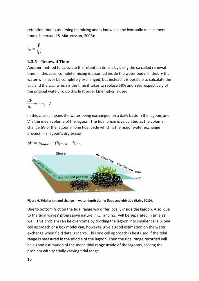
Figure 4. Tidal prism and change in water depth during flood and ebb tide (Bahr, 2010).

Due to bottom friction the tidal range will differ locally inside the lagoon. Also, due

to the tidal waves’ progressive nature, hflood and hebb will be separated in time as

well. This problem can be overcome by dividing the lagoon into smaller cells. A one

cell approach or a box model can, however, give a good estimation on the water

exchange when field data is scarce. This one cell approach is best used if the tidal

range is measured in the middle of the lagoon. Then the tidal range recorded will

be a good estimation of the mean tidal range inside of the lagoons, solving the

problem with spatially varying tidal range.

11

The water exchange coefficient for a tidal cycle, k, can be calculated if the lagoon

volume is known as:

However, if the tide is semi-diurnal the daily water exchange coefficient needs to

be multiplied by a factor 2:

Solving the first order kinematic differential equation yields:

The same equations can be used to calculate t99% with a change in the boundary

conditions to:

Then t99% becomes:

12

2.4 Sediment Transport Sediment transport processes in lagoons act to modify, retain and accumulate

sediments in various ways. These processes consist of four components. (Kjerfve,

1994)

1. erosion

2. transport

3. deposition and accumulation

4. diagenesis and consolidation

Sediment transport processes are produced when energy is dissipated by river

inflow, tides and waves or by forces such as wind. They change continuously due to

variations in weather and seasons. As these processes occur, the bottom geometry

or the shore configuration may be changed. (Kjerfve, 1994)

Since sediment transport processes are not constant within a lagoon the sediment

composition varies accordingly. Sediments may derive from various sources such as

streams, the ocean or from within the system. Lagoons that are fed by rivers

receive sediments varying from coarse sand to silt and clay. Coarser materials are

deposited soon after the river enters the lagoon and finer sediments are

transported further inside the lagoon where it deposits. (Kjerfve, 1994)

During the last century human populations have increased around lagoons,

resulting in human materials as a new source of sediments. Human material in this

case could be for example sewage sludge, garbage, hydrocarbons or industrial

waste. (Kjerfve, 1994)

The beach is constantly adjusting its profile as a natural dynamic response to the

ocean. Littoral drift, defined as the movement of sediments in the nearshore zone

by waves and currents, is one way to adjust. Littoral drift can be divided into two

processes: longshore transport and onshore-offshore transport. The longshore

transport is parallel and the onshore-offshore transport is perpendicular to the

shoreline (US Army Corps of Engineers, 1984). If littoral sediments accumulate at

an ocean inlet the lagoon can be closed off from the ocean, suppressing the tidal

water exchange (Kjerfve, 1994).

2.5 Water Quality Aspects Lagoons often present a high primary and secondary production rate, which makes

them attractive to aqua- and agriculture. This offers economical benefits to the

13

people in the proximity of the lagoon. At the same time, lagoons are facing a

multitude of water quality issues. (Kjerfve, 1994)

The main contributor to the deteriorating water quality in the lagoons is the

anthropogenic eutrophication. Nutrients are released into the water through

agricultural fertilizers and rest products, untreated sewage from nearby cities and

increased combustion of fossil fuel. Studies show that nitrogen has increased with

up to 50 times and phosphorous 18-180 times compared to pristine conditions.

(Junior, et al., 2012)

14

15

3 Mundaú-Manguaba Estuarine-Lagoon System

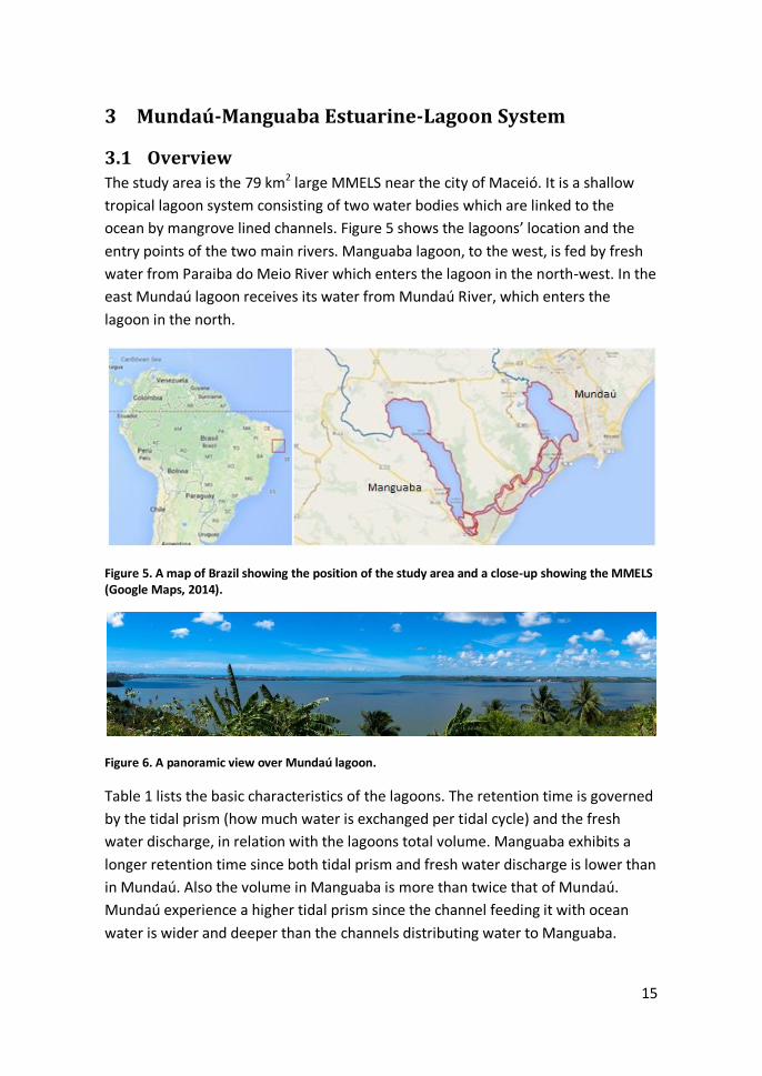
3.1 Overview The study area is the 79 km2 large MMELS near the city of Maceió. It is a shallow

tropical lagoon system consisting of two water bodies which are linked to the

ocean by mangrove lined channels. Figure 5 shows the lagoons’ location and the

entry points of the two main rivers. Manguaba lagoon, to the west, is fed by fresh

water from Paraiba do Meio River which enters the lagoon in the north-west. In the

east Mundaú lagoon receives its water from Mundaú River, which enters the

lagoon in the north.

Figure 5. A map of Brazil showing the position of the study area and a close-up showing the MMELS (Google Maps, 2014).

Figure 6. A panoramic view over Mundaú lagoon.

Table 1 lists the basic characteristics of the lagoons. The retention time is governed

by the tidal prism (how much water is exchanged per tidal cycle) and the fresh

water discharge, in relation with the lagoons total volume. Manguaba exhibits a

longer retention time since both tidal prism and fresh water discharge is lower than

in Mundaú. Also the volume in Manguaba is more than twice that of Mundaú.

Mundaú experience a higher tidal prism since the channel feeding it with ocean

water is wider and deeper than the channels distributing water to Manguaba.

16

Mundaú Manguaba

Area [km2] 24 43

Volume [106 m

3] 43 97.7

Average depth [m] 1.5 2.1

Tidal range [m] 0.2 0.03

Tidal prism [106 m3] 17.3 6.1

Average freshwater discharge [m3/s] 35 28

Retention time [days] 16 36

Table 1. Table showing basic parameters regarding the lagoons (Oliveira & Kjerfve, 1993).

A 12 km2 large channel system connects the two lagoons to the ocean via a 250 m

wide inlet. Due to littoral drift the inlet has been closed off during three events

throughout the last century (Oliveira & Kjerfve, 1993).

3.2 Climatology The lagoon system is situated in a tropical semi-humid climate with well defined

dry and wet seasons. The dry season lasts from December to March and the wet

season from May to August. (Oliveira & Kjerfve, 1993)

Climate data was collected online

from HidroWeb’s webpage at two

measuring stations in the vicinity of

the lagoons. Figure 7 shows the

locations of these stations, which

were used to collect the weather data

presented below.

The average annual precipitation and

evaporation is 1772 mm and 1138

mm respectively. June receives a

maximum monthly precipitation of

285 mm and November a minimum of

45 mm. In the period October to

February the evaporation is higher

than the precipitation.

Figure 7. Location of the weather stations used for the calculation of weather conditions (Google Maps, 2014).

17

Figure 8. Mean annual precipitation and evaporation during 1962-1997 (HidroWeb, 2013).

The direction of the wind is south-east in the wet season and east in the dry

season, in both cases with an average speed of 6 m/s. The water temperature has a

monthly average value of maximum 31 °C in the dry season and a minimum of 25

°C in the wet season. (Oliveira & Kjerfve, 1993). The air temperature varies over the

year with lower temperatures during the wet season. Figure 9 shows the variations

in air temperature over the year.

Figure 9. Mean air temperature in the MMELS during 1962-1997 (HidroWeb, 2013).

0

50

100

150

200

250

300

Jan Feb Mar Apr May Jun Jul Aug Sep Oct Nov Dec

[mm

] Mean Annual Precipitation and Evaporation

(1962-1997)

Precipitation

Evaporation

23

23.5

24

24.5

25

25.5

26

26.5

Jan Feb Mar Apr May Jun Jul Aug Sep Oct Nov Dec

Tem

per

atu

re [C

°]

Mean Monthly Air Temperature (1962-1997)

Air temperature

18

3.3 Hydrographic Conditions and Morphology

3.3.1 Bathymetry

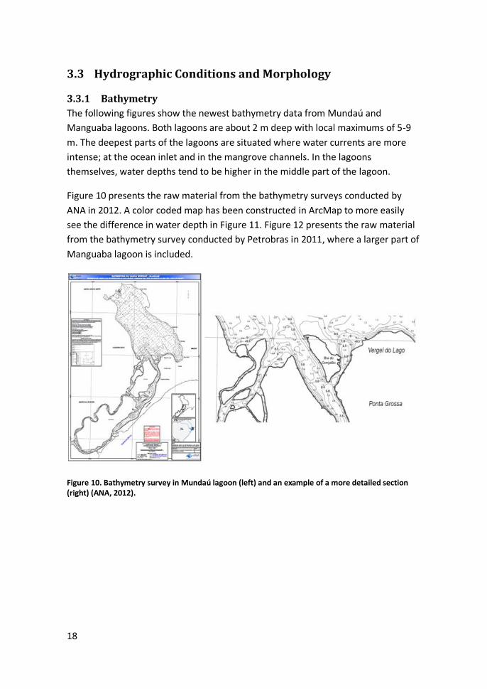
The following figures show the newest bathymetry data from Mundaú and

Manguaba lagoons. Both lagoons are about 2 m deep with local maximums of 5-9

m. The deepest parts of the lagoons are situated where water currents are more

intense; at the ocean inlet and in the mangrove channels. In the lagoons

themselves, water depths tend to be higher in the middle part of the lagoon.

Figure 10 presents the raw material from the bathymetry surveys conducted by

ANA in 2012. A color coded map has been constructed in ArcMap to more easily

see the difference in water depth in Figure 11. Figure 12 presents the raw material

from the bathymetry survey conducted by Petrobras in 2011, where a larger part of

Manguaba lagoon is included.

Figure 10. Bathymetry survey in Mundaú lagoon (left) and an example of a more detailed section (right) (ANA, 2012).

19

Figure 11. Color coded water depths in Mundaú lagoon according to the bathymetry survey.

Figure 12. Bathymetry survey of Manguaba lagoon (Petrobas, 2011).

3.3.2 Sediments

For Mundaú lagoon, sediment maps have been acquired. In Figure 13 the

sediments are described as a percentage of sand (left) and clay (right) found in the

bottom sediments. The maps show a concentration of mud in the middle parts of

20

the lagoon, where water velocities are at their lowest. Sand sediments are

predominately found in the north-west, where the lagoon meets the river, and in

the south where the mangrove channel enters the lagoon.

Figure 13. Sediment survey in Mundaú lagoon with percentage of sand (left) and clay (right) found in the bottom sediments (ANA, 2012).

For Manguaba lagoon no sediment maps were acquired, but an investigation of its

sediments was performed in 1988. The report shows that the bottom sediments

mainly consists of clay except in three places; near the channel junction in the

south, a 2 km2 area in the northern part of the lagoon and a 1 km2 area of medium-

size sand near the Paraiba do Meio´s inlet (Oliveira & Kjerfve, 1993).

3.4 Water Exchange

3.4.1 Fresh Water Inflow

One river is supplying each of the lagoons with fresh water; Paraiba do Meio in

Manguaba lagoon and River Mundaú in Mundaú lagoon. The flow in the rivers

varies with the wet and dry seasons. Average flow in the rivers during dry season is

approximately 10 m3/s but during long periods of draught the rivers cease to

provide fresh water. During the wet season average flows for Paraiba do Meio and

Mundaú River is 39 m3/s and 67 m3/s, respectively. Intense flows can reach 98 m3/s

21

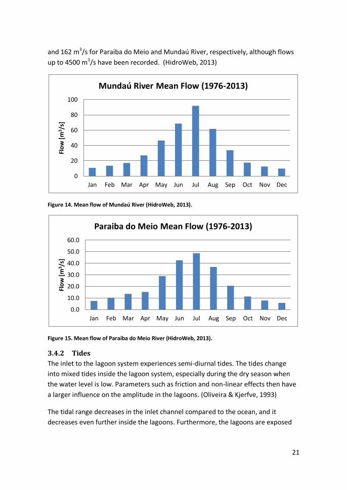
and 162 m3/s for Paraiba do Meio and Mundaú River, respectively, although flows

up to 4500 m3/s have been recorded. (HidroWeb, 2013)

Figure 14. Mean flow of Mundaú River (HidroWeb, 2013).

Figure 15. Mean flow of Paraiba do Meio River (HidroWeb, 2013).

3.4.2 Tides

The inlet to the lagoon system experiences semi-diurnal tides. The tides change

into mixed tides inside the lagoon system, especially during the dry season when

the water level is low. Parameters such as friction and non-linear effects then have

a larger influence on the amplitude in the lagoons. (Oliveira & Kjerfve, 1993)

The tidal range decreases in the inlet channel compared to the ocean, and it

decreases even further inside the lagoons. Furthermore, the lagoons are exposed

0

20

40

60

80

100

Jan Feb Mar Apr May Jun Jul Aug Sep Oct Nov Dec

Flo

w [

m3 /

s]

Mundaú River Mean Flow (1976-2013)

0.0

10.0

20.0

30.0

40.0

50.0

60.0

Jan Feb Mar Apr May Jun Jul Aug Sep Oct Nov Dec

Flo

w [

m3 /

s]

Paraiba do Meio Mean Flow (1976-2013)

22

to a pronounced spring-neap cycle. During the wet season the tidal amplitudes

have a greater range due to the greater water depths. (Oliveira & Kjerfve, 1993)

The channel system reduces the tidal range in the lagoons to a great extent. This is

usually the case for choked lagoons, where tidal water-level fluctuations could be

reduced to 1 % or less compared to the coastal tide. During the dry season the

filtering effect is more distinct in the MMELS due to lower water levels and

consequently higher friction. (Oliveira & Kjerfve, 1993)

3.5 Sediment Transport and Morphological Change The inlet switches positions dynamically due to currents and has closed off the

lagoons from the ocean completely at three times the last century; in 1910, 1930

and 1939 (Oliveira & Kjerfve, 1993).

Sedimentation near the original ocean inlet has affected Manguaba lagoon´s ability

to drain itself during heavy rains. To avoid flooding in the Barra Nova area a new

ocean inlet was constructed in 2011. Although it has succeeded to prevent further

flooding, it has decreased the hydraulic communication between the two lagoons.

(Prefeitura Municipal de Marechal Deodoro, 2011)

Figure 16 shows the position of the main ocean inlet, the newly constructed ocean

inlet at Barra Nova and the location of the channel which has been filled by

sediments. This has reduced the hydraulic communication between the lagoons.

Figure 16. Map showing the original ocean inlet (1), the new ocean inlet constructed in Barra Nova (2) and the closed of channel in between the two lagoons (3) (Google Maps, 2014).

23

3.6 Water Quality The lagoon system experiences various types of water quality issues, where

pollution and salinity fluctuations are the most prominent. It is heavily impacted by

waste from the domestic sewage and sugar cane industry along the rivers.

To simplify the process of harvesting sugar canes, the leaves are burned off, leaving

only the stalks. Great volumes of water are then withdrawn from the rivers to clean

the ash of the sugar cane stalks. This water is then released back into the river with

a BOD-content of up to 450 mg/l. Vinhoto is another byproduct created when sugar

cane juice is turned into methanol. About 12 liters of vinhoto is produced for every

liter of methanol. Although the volume of vinhoto released in the rivers is far less

than that of the ash rich water from the cleaning process, it is a more potent

pollutant with BOD-values reaching 45,000 mg/l. (Lages & Lopes, 2005)

Another source of pollution is the untreated urban sewage from the city of Maceió

and from other small cities along the rivers. It is estimated that in the city Maceió,

with a population of 1.2 million, only 10% of the wastewater is treated (Oliveira &

Kjerfve, 1993). However Fragoso Jr. (2014) suggests that currently almost 35 % is

collected but still only 10 % is treated. Pipes that discharge untreated sewage into

the lagoons are very common.

Figure 17. Untreated sewage discharged directly into the lagoon.

24

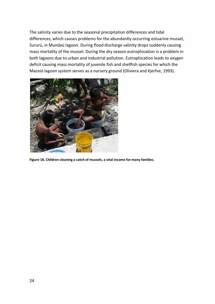
The salinity varies due to the seasonal precipitation differences and tidal

differences, which causes problems for the abundantly occurring estuarine mussel,

Sururú, in Mundaú lagoon. During flood discharge salinity drops suddenly causing

mass mortality of the mussel. During the dry season eutrophication is a problem in

both lagoons due to urban and industrial pollution. Eutrophication leads to oxygen

deficit causing mass mortality of juvenile fish and shellfish species for which the

Maceió lagoon system serves as a nursery ground (Oliviera and Kjerfve, 1993).

Figure 18. Children cleaning a catch of mussels, a vital income for many families.

25

4 Field Measurements

4.1 Previous Studies Numerous studies about the MMELS were carried out in the 70’s and 80’s. For

example, an environmental description was provided and studies about both the

Sururú mussel and nekton were performed. The Instituto Nacional de Pesquisas

Hidráulicas (INPH) investigated the lagoon complex thoroughly during both the wet

season and the dry season in 1984-1985. (Oliveira & Kjerfve, 1993). Among other

things, bathymetry data is available from this investigation.

A new bathymetry survey was performed for Mundaú in 2012 by ANA. A

bathymetric survey consists of two components: a planimetric and an altimetric

position. The planimetric positioning in Mundaú Lake was performed with a

technique which in this case provided an accuracy of more than five meters for the

planimetric positioning. The depth determination (altimetry) was performed using

digital echo sounders with an accuracy of 1% (ANA, 2012). However it is uncertain if

this high accuracy was possible to achieve during the survey. The previous year a

similar survey was performed in Manguaba by Petrobras (2011).

Universidade Federal de Alagoas also performed a campaign in 2012 measuring

pressure, temperature and actual conductivity at two locations. The chosen points

are located close to each other and near to the ocean inlet.

4.2 Experimental Setup and Procedure A new campaign was performed 15th of February 2014 as a part of this project. Two

sensors of the model Aqua Troll 200 (see Appendix I) were placed in the lagoon

system. The pressure, temperature and actual conductivity of the water were

measured every fifteen minutes and from this data depth and salinity, among other

things, were calculated automatically. The sensors were retrieved at 12th of March

after about three and a half weeks of measurements.

When the campaign was performed in 2012 both sensors were placed close to each

other near the ocean inlet. This time one sensor was placed inside each lagoon to

obtain a better understanding of the water level variations in the lagoons (Figure

19).

26

Figure 19. Placement of the sensors during the field campaign (Google Maps, 2014).

One problem when performing campaigns is the risk of losing the sensors due to

theft. In order to avoid this problem the location of the sensors were chosen with

great care. One was placed close to a restaurant where the owner could safeguard

it, the other in the private backyard of a residence.

Figure 20. Placement of the sensor in Manguaba lagoon.

27

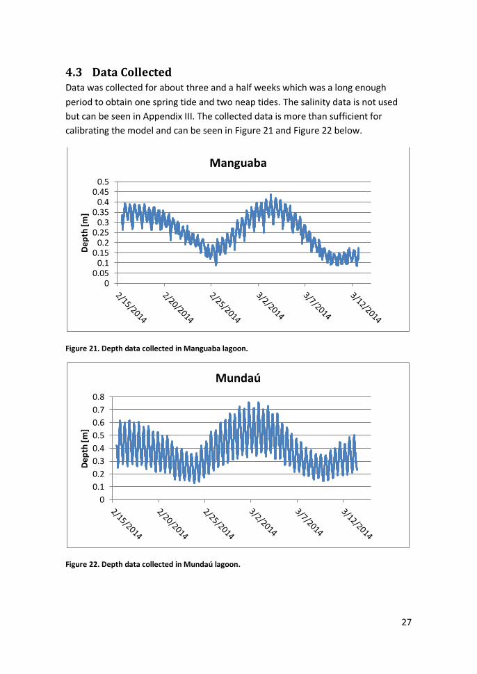
4.3 Data Collected Data was collected for about three and a half weeks which was a long enough

period to obtain one spring tide and two neap tides. The salinity data is not used

but can be seen in Appendix III. The collected data is more than sufficient for

calibrating the model and can be seen in Figure 21 and Figure 22 below.

Figure 21. Depth data collected in Manguaba lagoon.

Figure 22. Depth data collected in Mundaú lagoon.

0 0.05

0.1 0.15

0.2 0.25

0.3 0.35

0.4 0.45

0.5

Dep

th [m

]

Manguaba

0

0.1

0.2

0.3

0.4

0.5

0.6

0.7

0.8

Dep

th [m

]

Mundaú

28

29

5 The IPH-ECO Model

5.1 Basic Theory IPH-ECO is based on a finite element approach which gives a two dimensional

depth-integrated solution to the continuity and momentum equations. The

mathematical formulation of the program is based on Navier-Stokes equation. By

assuming that the horizontal flows are much greater than the vertical ones, Navier-

Stokes equation can be depth-integrated to form the shallow water equations. To

depth-integrate the program uses two boundary conditions; wind shear stress at

the free water surface and frictional forces at the bottom. (Pereira, et al., 2013)

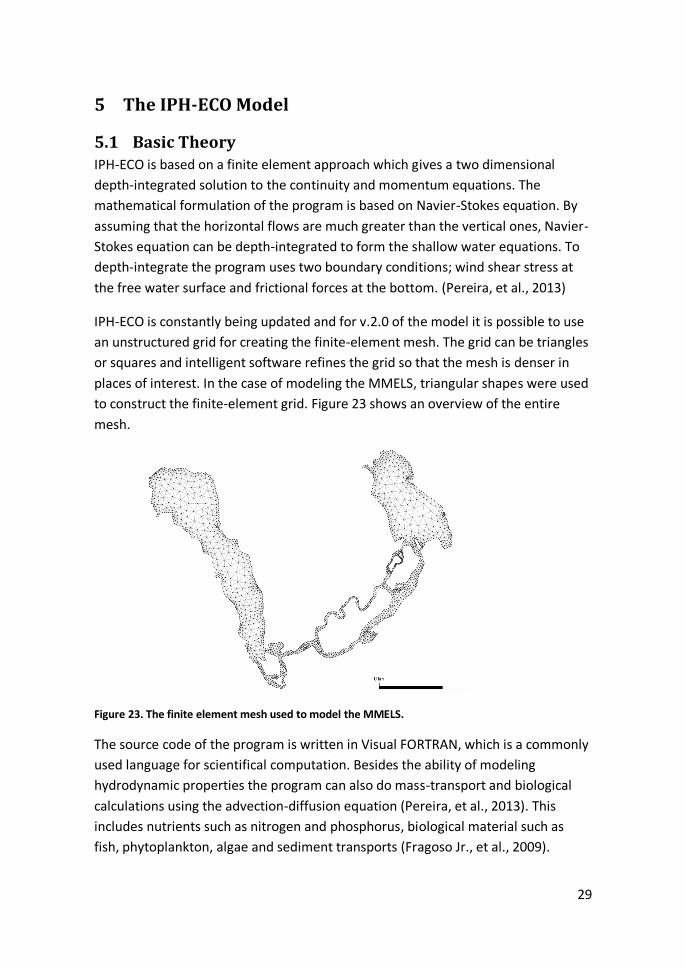
IPH-ECO is constantly being updated and for v.2.0 of the model it is possible to use

an unstructured grid for creating the finite-element mesh. The grid can be triangles

or squares and intelligent software refines the grid so that the mesh is denser in

places of interest. In the case of modeling the MMELS, triangular shapes were used

to construct the finite-element grid. Figure 23 shows an overview of the entire

mesh.

Figure 23. The finite element mesh used to model the MMELS.

The source code of the program is written in Visual FORTRAN, which is a commonly

used language for scientifical computation. Besides the ability of modeling

hydrodynamic properties the program can also do mass-transport and biological

calculations using the advection-diffusion equation (Pereira, et al., 2013). This

includes nutrients such as nitrogen and phosphorus, biological material such as

fish, phytoplankton, algae and sediment transports (Fragoso Jr., et al., 2009).

30

5.2 Numerical Formulation As mentioned before, two boundary conditions are used to depth integrate the

Navier-Stokes equation; wind shear stress at the free water surface and bottom

friction. These parameters are defined by (Pereira, et al., 2013):

and

where Av is the vertical eddy viscosity,

and

are the horizontal velocity

components along the water column, τ is the wind shear stress and γ is the bottom

friction. The letters u and v denotes the water velocity in x- and y-direction. The

wind shear stress is formulated as:

where CD is a drag coefficient, W denotes the wind speed as a vector, and is

the normalized vector W.

Bottom friction is determined by:

where C is the Chezy coefficient and H is the total water depth according to H=h+η.

The momentum equation and continuity equation that IPH-ECO has to solve can be

formulated according to (Pereira, et al., 2013):

where Ah is the horizontal eddy viscosity coefficient, f denotes the Coriolis

parameter and η is the total water depth. All other variables are explained above.

31

5.3 Model Input and Setup The model is run for 15 days which is considered sufficient for both calibration and

running scenarios. Running the model for more than 15 days would take too long

to compute and would not contribute much to the results. Two of these days are

needed to run in the model to obtain a higher stability. Therefore the starting date

of the model is 13th of February while the sensor data starts on 15th o February.

The most important input data for running the IPH-ECO model are bathymetry,

tidal variations, Chezy coefficient and inflow from the rivers. The precipitation is set

to zero since the simulation period is in the dry season. Other data, such as effects

of wind, evaporation and solar radiation are also set to zero in order to simplify the

model.

5.3.1 Bathymetry

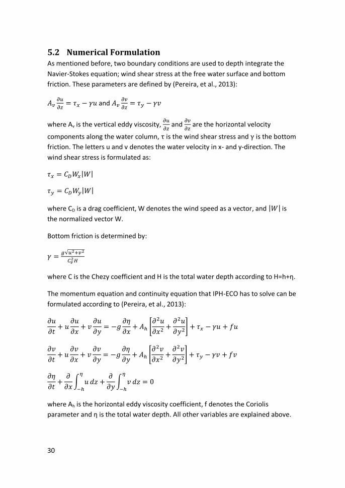
New bathymetry surveys were performed recently for both lagoons. The

bathymetry of Mundaú lagoon has already been converted into a shape file in

ArcGIS during a previous study. For Manguaba lagoon Figure 12 with depth

contours and coordinates was the only available data from the bathymetry survey.

In order to use this information in the model it was therefore necessary to convert

it into a more appropriate file format, a shape file, using ArcGIS. The figure does

however not contain all the information needed. A large part of the lower section

in Manguaba and its channel system is missing. Therefore, to complement the

figure, a map of the area needed to be imported from Google Maps in order to

create a complete shoreline.

The georeferencing system used during the bathymetry survey was SIRGAS2000

24S. Google Maps uses WSG84 in their maps, but both maps could be aligned using

ArcMaps built in Georeferencing tool. The already existing bathymetry of Mundaú

lagoon was thereafter inserted into the same shape file as the two

abovementioned figures and georeferenced to match Manguaba.

32

Figure 24. Map showing the area of the bathymetry survey during 2011 (left) and the missing bathymetry (right) (Google Maps, 2014).

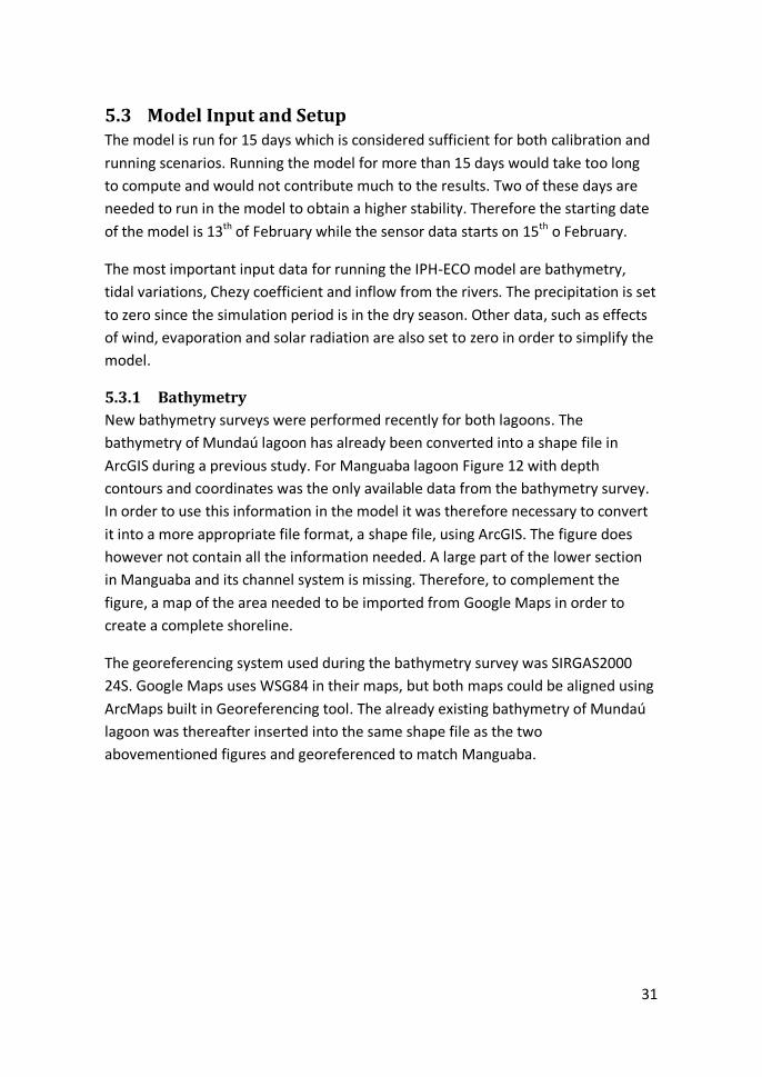
When the georeferencing was complete polylines were drawn along the depth

contours and they were assigned attributes stating the correct depth. The shoreline

was plotted with a polyline and assigned the depth 0 m. All polylines were later

split into points in order to construct a point file. The figure imported from Google

Maps solved the problem with creating a shoreline, but information about the

depth in this area was still missing. After consulting with Fragoso Jr. (2014), values

from 1984 were used to fill in the missing values. This was however not sufficient

since there were very few points in south of Manguaba and its channel. The

solution was to add more points in this area and estimate their depths.

Figure 25. New bathymetry including data from 1984 in southern Manguaba (left) and the completed point-file for the whole MMELS with added points (right).

When all the data was merged together into a point file it was possible to convert

the bathymetry into an unstructured grid using the program JANET. This file was

then used as a boundary condition in IPH-ECO.

33

5.3.2 Tide

There was data available about the tidal variations in Maceió harbor, but only

regarding the high and the low tides. More values were necessary to run the model

and for that reason the program WTides was used. It uses harmonic analysis to

predict tide throughout the world and shows the results in a graph. Maceió (9°40.0’

S, 35°43.0’ W) was chosen as a target location and the values were read from the

graph hourly during the chosen time period. The values obtained from the program

were then compared with the values from the harbor and they matched well. The

lagoon system is situated some distance away from the harbor and after consulting

with professor Fragoso Jr. (2014) a 10 % reduction was applied to the data. The

10 % reduction is based on experience rather than scientific data, but during past

calibrations of IPH-ECO, this reduction has shown to be a good estimation.

5.3.3 Inflow

The inflows from Mundaú River and Paraíba do Meio were retrieved from ANA. The

inflow values have been measured two to three times per day during the chosen

period at the measuring stations Atalaia and Rio Largo which can be seen below in

Figure 26.

Figure 26. Flow measurement station for Mundaú River and Paraiba do Meio respectively (ANA, 2012).

5.3.4 Chezy Coefficients

IPH-ECO was originally constructed to only allow for one uniform Chezy coefficient

in the whole lagoon system. To more realistically represent reality the program was

rewritten to read a more complex file, where different Chezy coefficients could be

assigned to different areas in the lagoons. Using available information on

34

sediments in l Mundaú and Manguaba (see Chapter 3.3.2) and tables for estimation

of Manning coefficients, a more complex picture of Chezy could be represented.

There are numerous methods developed for estimating the Manning roughness

coefficient, but the one best suited for this situation was found to be Cowan´s

method (Brisbane City Council, u.d.)

Lagoon Mostly Sand

Lagoon Mostly Clay

Manning Manning

Material Mostly sand

0.024 Material Mostly clay

0.02

Irregularity Smooth 0 Irregularity Smooth 0

Variation cross-section

None 0 Variation cross-section

None 0

Obstruction Minor 0.002 Obstruction Minor 0.002

Vegetation Minor 0.01 Vegetation None 0

Meandering None 0 Meandering None 0

Σ 0.036 Σ 0.022

Table 2. Estimation of Manning coefficients for mostly sand and mostly clay.

Since the IPH-ECO model uses Chezy and not Manning coefficient these values

need to be converted. The relationship between Chezy and Manning is given by:

where C is the Chezy coefficient, n is the Manning roughness coefficient and R is

the hydraulic radius. The hydraulic radius is here taken as the water depth. The

average depth is 1.5 m in Mundaú and 2.1 m in Manguaba, but the channels are

deeper. For that reason the hydraulic radius is estimated to be 2.5 m. Using this

method, two extreme values can be calculated. The transitional zones which are

neither mainly sand nor clay will be subjected to estimations somewhere between

the two extreme values.

Bottom Sediments Chezy

Mostly sand 32

Mostly clay 53

Table 3. Typical maximum and minimum values for Chezy in the MMELS.

35

Since there is very little available data for Manguaba lagoon the bottom sediments

are assumed to consist of mostly clay in the lagoon itself and of mostly sand in the

channel system. The estimated Chezy distribution used in the IPH-ECO model can

be seen in Figure 27.

Figure 27. Estimated Chezy values in the MMELS.

5.4 Calibration Process The first step in the calibration process was to test the new version of the IPH-ECO

program. Version 1.0 of IPH-ECO has been used before with data from 1984 and

therefore it seemed logical to start off by testing the same data from 1984 in v.2.0

of the program and compare the results. The reason for this step in the calibration

process was to ensure that the new version with the unstructured grid gave the

same results as the old version of the model, given the same input data.

Results from three points are available from the first version of the program; one in

Mundaú, one in Manguaba and one near the river mouth. Consequently the same

points were chosen for the simulation in the second version of the program. The

36

results (see Appendix II) match very well which shows that the second version of

the program is working correctly.

The next step was to use the available data from the campaign performed in 2012

by UFAL in order to calibrate the model roughly while waiting for the new data. The

problem however, as mentioned before, was that the placement of the sensors

was not ideal. Therefore the model was mainly calibrated using the new data from

February and March 2014 which is in the dry season.

When calibrating the model the aim was to match the water levels from the

sensors as much as possible. In order to do so, two parameters were changed; the

bathymetry values and the Chezy coefficients. The bathymetry was incomplete

which gave room for some interpretation. The Chezy coefficients were an

estimation using Cowan´s method and they were changed continuously when

comparing to sensor data.

It is also possible to calibrate the model regarding water velocities; however no

such equipment was available for a field campaign.

5.4.1 Estimation of Correlation

There are various ways to determine how well the modeled data matches the

sensor values. During the calibration process a visual determination was used until

satisfying results were obtained. Thereafter three more mathematical methods

were used.

The Pearson correlation coefficient, r, represents the degree of linear relationship

between pairs of variables (King, et al., 2011):

where X is the measured value and Y is the modeled value. For sinusoidal curves,

this parameter describes how well the phases match each other, but says little

about amplitude or displacement.

RMS (Root Mean Square) is a statistical method for calculating quadratic mean

values. In this case, the magnitude of deviation in water depth between sensor

data and computer model was compared for each time step, and then presented as

a mean deviation value according to:

37

where n is the number of data points for the whole calibration period and Δx is the

error between the model and the sensor for each data point.

The mean tidal range for the calibration period was also calculated to give an

estimation of how well the amplitudes match between model and sensor.

The proportional correlation (ρ) between each data point can be calculated

according to:

To visualize the result, the correlation can be plotted in a correlation diagram to

see how the correlation changes with time.

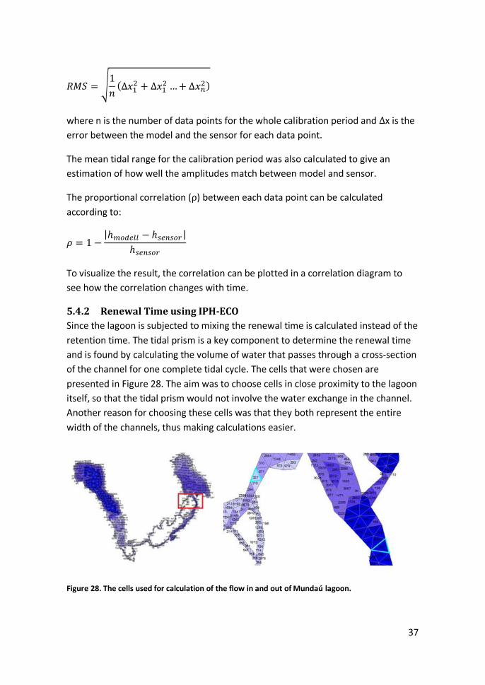
5.4.2 Renewal Time using IPH-ECO

Since the lagoon is subjected to mixing the renewal time is calculated instead of the

retention time. The tidal prism is a key component to determine the renewal time

and is found by calculating the volume of water that passes through a cross-section

of the channel for one complete tidal cycle. The cells that were chosen are

presented in Figure 28. The aim was to choose cells in close proximity to the lagoon

itself, so that the tidal prism would not involve the water exchange in the channel.

Another reason for choosing these cells was that they both represent the entire

width of the channels, thus making calculations easier.

Figure 28. The cells used for calculation of the flow in and out of Mundaú lagoon.

38

IPH-ECO does not output flows in the cells directly, only u and v velocity

components. These can be summarized into one resultant velocity. The depth of

the cells is acquired directly from IPH-ECO and the channel width can be measured

in ArcGIS. It is then possible to calculate the flow (see Appendix IV).

Cell 586 Cell 207

Depth 2.73 0.21

Width 205 127

Area 559.65 26.67

Table 4. Calculation of cross-section areas for each cell respectively.

To calculate the tidal prism the volume for each time step is calculated and

summarized according to:

where n is the number of time steps needed to complete a full tidal cycle, and tk is

1800 seconds. The reason for summarizing the full tidal cycle is that the incoming

and outgoing water differs slightly in volume. Dividing by two gives the mean value

for the tidal prism. Lastly, the water exchange coefficient is calculated together

with t50% and t99%.

5.4.3 Renewal Time using Sensor Readings

In this simple method the renewal time for Mundaú and Manguaba lagoons will be

calculated on the 16th of February 2014 and on the 23rd of February 2014. These

dates represent one spring tide and one neap tide. Since it is dry season during

these dates, river inflow is negligible compared to lagoon volumes. Groundwater

seepage is also neglected, since no data is available to quantify this. Also, it is of

lesser importance since it is many magnitudes smaller than the tidal prism in arid

climates. Groundwater seepage may have a larger impact on the results during wet

season when precipitation is high.

The purpose of calculating the renewal time using sensor readings is to see if it

gives a good enough estimation or if it is necessary to use a complex program such

as IPH-ECO.

39

The most important water exchange process is that done by the tide. The sensors

give a height difference, and the volume of the tidal prism can then be calculated

using the entire lagoon area. The surface area of the Mundaú and Manguaba

lagoons are 24 km2 and 43 km2 respectively. The tidal prism is then calculated

according to the method presented in Chapter 2.3.5.

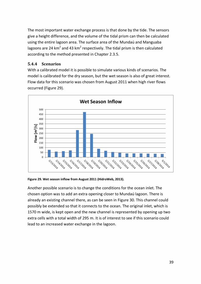
5.4.4 Scenarios

With a calibrated model it is possible to simulate various kinds of scenarios. The

model is calibrated for the dry season, but the wet season is also of great interest.

Flow data for this scenario was chosen from August 2011 when high river flows

occurred (Figure 29).

Figure 29. Wet season inflow from August 2011 (HidroWeb, 2013).

Another possible scenario is to change the conditions for the ocean inlet. The

chosen option was to add an extra opening closer to Mundaú lagoon. There is

already an existing channel there, as can be seen in Figure 30. This channel could

possibly be extended so that it connects to the ocean. The original inlet, which is

1570 m wide, is kept open and the new channel is represented by opening up two

extra cells with a total width of 295 m. It is of interest to see if this scenario could

lead to an increased water exchange in the lagoon.

0

50

100

150

200

250

300

350

400

450

500

Flo

w [

m3 /

s]

Wet Season Inflow

40

Figure 30. The location of the new ocean inlet (Google Maps, 2014).

41

6 Results

6.1 Calibration Results After calibrating the IPH-ECO model the results in Figure 31 and Figure 32 were

obtained:

Figure 31. The calibration results for Manguaba.

Many different configurations were used for Manguaba in order to get a good

match. Chezy values of 53 were applied for both the lagoon and the channel,

suggesting that all bottom sediments consist of clay. Depths of about five meters

where tried to get a higher tidal range in the lagoon, but without success.

Improvements of sediment and bathymetry surveys may be the answer to this

problem, but it cannot be ruled out that some numerical error is present in the

model. It can be that the inlet cell from the channel into southern Manguaba is too

narrow to transport this amount of water.

0

0.05

0.1

0.15

0.2

0.25

0.3

0.35

0.4

0.45

Dep

th [m

]

Manguaba

Sensor

Model

42

Figure 32. The calibration results for Mundaú.

Mundaú was easily calibrated due to the detailed bathymetry and sediment

information. Only a small adjustment of Chezy coefficients was necessary. When

calibrating Manguaba the results for Mundaú remained the same, suggesting that

the two lagoons are working independently of each other. This was expected since

they have separate inlets at present.

Visually Mundaú seems to better match the sensor reading than Manguaba. To

objectively assess this, the parameters in Chapter 5.4.1 were used to quantify the

correlation.

Tidal Range Sensor [m]

Tidal Range Model [m]

Pearson Correlation [%]

RMS [m]

Mundaú 0.301 0.303 93.3 0.050

Manguaba 0.075 0.035 97.5 0.039

Table 5. Different methods of estimating correlation.

Pearson Correlation shows good correlation of the tidal phases. The deviation of

tidal range in Manguaba is evident when analyzing mean tidal range. RMS appears

to be lower in Manguaba, but in relation to tidal range, the error is proportionally

greater. The correlation diagram highlights Manguaba’s bad correlation during the

neap tide period.

0

0.1

0.2

0.3

0.4

0.5

0.6

0.7

0.8

De

pth

[m]

Mundaú

Sensor

Model

43

Figure 33. Correlation diagram.

After assessing the above mentioned parameters it was decided to continue to run

scenarios and plot vector fields for Mundaú only because of Manguaba’s bad

correlation and large deviation of tidal range. In addition, Mundaú is of more

interest to model in this study since it is located closer to the city of Maceió.

6.2 Scenarios

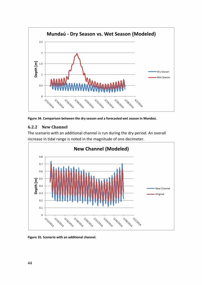
6.2.1 Wet Season

This scenario is simulated using IPH-ECO to forecast water levels during high runoff.

During the wet season the river discharge is high, sometimes reaching flows over

400 m3/s (see Chapter 5.4.4). This results in a peak in water level when simulating

this scenario. The water level rises from 0.5 m to 2.0 m compared to the dry

season. During peak flow the tidal variation is less prominent and it takes about 24

hours for the water level to recede afterwards. The general water level during the

wet season is approximately 0.2 m higher than during the dry season.

0

10

20

30

40

50

60

70

80

90

100 C

orr

ela

tio

n [

%]

Correlation Diagram

Mundau

Manguaba

44

Figure 34. Comparison between the dry season and a forecasted wet season in Mundaú.

6.2.2 New Channel

The scenario with an additional channel is run during the dry period. An overall

increase in tidal range is noted in the magnitude of one decimeter.

Figure 35. Scenario with an additional channel.

0

0.5

1

1.5

2

2.5

De

pth

[m]

Mundaú - Dry Season vs. Wet Season (Modeled)

Dry Season

Wet Season

0

0.1

0.2

0.3

0.4

0.5

0.6

0.7

0.8

Dep

th [m

]

New Channel (Modeled)

New Channel

Original

45

6.3 Renewal Time The renewal time during the dry season has been calculated using both IPH-ECO

and sensor readings. Moreover, the renewal time has been calculated for the

scenario with the new channel, also during the dry season, thus making a

comparison possible.

6.3.1 IPH-ECO

Tidal prism and renewal time for Mundaú is calculated using the IPH-ECO model

during 16th of February (spring tide) and 23rd of February (neap tide). No renewal

time is calculated for Manguaba since it is not calibrated well enough.

Tidal prism [106 m3] rv t50% [days] t99% [days]

16 Feb 5.3 0.247 2.8 18.7

23 Feb 2.4 0.110 6.3 42.0

Table 6. Renewal time calculated with the IPH-ECO model.

6.3.2 Additional Ocean Inlet

If a new channel is constructed the renewal time will decrease in Mundaú lagoon

compared to only having the original opening to the ocean. This is due to the

increase of tidal range inside the lagoon.

Tidal prism [106 m3] rv t50% [days] t99% [days]

16 Feb 7.4 0.345 2.0 13.4

23 Feb 3.4 0.156 4.4 29.4

Table 7. Renewal time for additional ocean inlet.

6.3.3 Sensor Readings

In general this method using sensor readings returns a higher tidal prism and a

lower renewal time than the IPH-ECO model. This method overestimates the tidal

prism because of the placement of the sensors. Due to tidal filtering the tidal range

is smaller in the northern part of the lagoon. Since the sensors are more located in

the south or middle part of the lagoons, they will give a too high tidal range.

Since the tidal range in Manguaba is small the renewal time is substantially longer

than in Mundaú.

46

Mundaú

Low tide [m]

High tide [m]

Δh [m]

Tidal prism

[106 m3]

rv t50% [days]

t99% [days]

16 Feb 0.256 0.616 0.360 8.6 0.402 1.7 11.5

23 Feb 0.126 0.355 0.229 5.5 0.256 2.7 18.0

Table 8. Renewal time in Mundaú calculated with the sensor readings.

Manguaba

Low tide [m]

High tide [m]

Δh [m]

Tidal prism

[106 m3]

rv t50%

[days] t99%

[days]

16 Feb 0.267 0.375 0.108 4.6 0.095 7.3 96.9

23 Feb 0.152 0.240 0.088 3.8 0.077 8.9 118.9

Table 9. Renewal time in Manguaba calculated with the sensor readings.

6.4 Vector Fields The process of plotting vector fields was rather problematic. For every plotted

vector, a cell from the unstructured grid needed to be chosen and its coordinates

had to be determined. Thereafter all the flow values had to be put in manually

before a plot could be constructed. Consequently the number of vectors had to be

reduced to 20. This is the reason why the resulting vector fields are not particularly

detailed. They do however give an overall view of the direction and magnitude of

the flow for the different scenarios.

Figure 36 shows the inflow to the lagoon during high tide where currents in the

range of 0.4 m/s can be found in the inlet. The strongest currents are

predominantly found in the western part of the lagoon. The south eastern part of

the lagoon displays only small water velocities, which suggests a lesser tidal mixing

in this area.

47

Figure 36. Vector fields dry season during tidal inflow.

During the outflow in Figure 37 the situation is reversed and the strongest currents

are found in the eastern part of the lagoon. No effect of fresh water inflow in the

northern part can be seen, since river flow is negligible during the dry period.

Water currents reach a speed of nearly 0.1 m/s during the outgoing tide.

Figure 37. Vector fields dry season during tidal outflow.

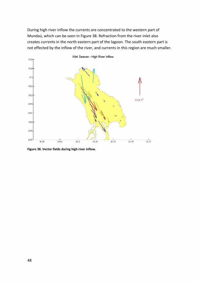
48

During high river inflow the currents are concentrated to the western part of

Mundaú, which can be seen in Figure 38. Refraction from the river inlet also

creates currents in the north eastern part of the lagoon. The south eastern part is

not effected by the inflow of the river, and currents in this region are much smaller.

Figure 38. Vector fields during high river inflow.

49

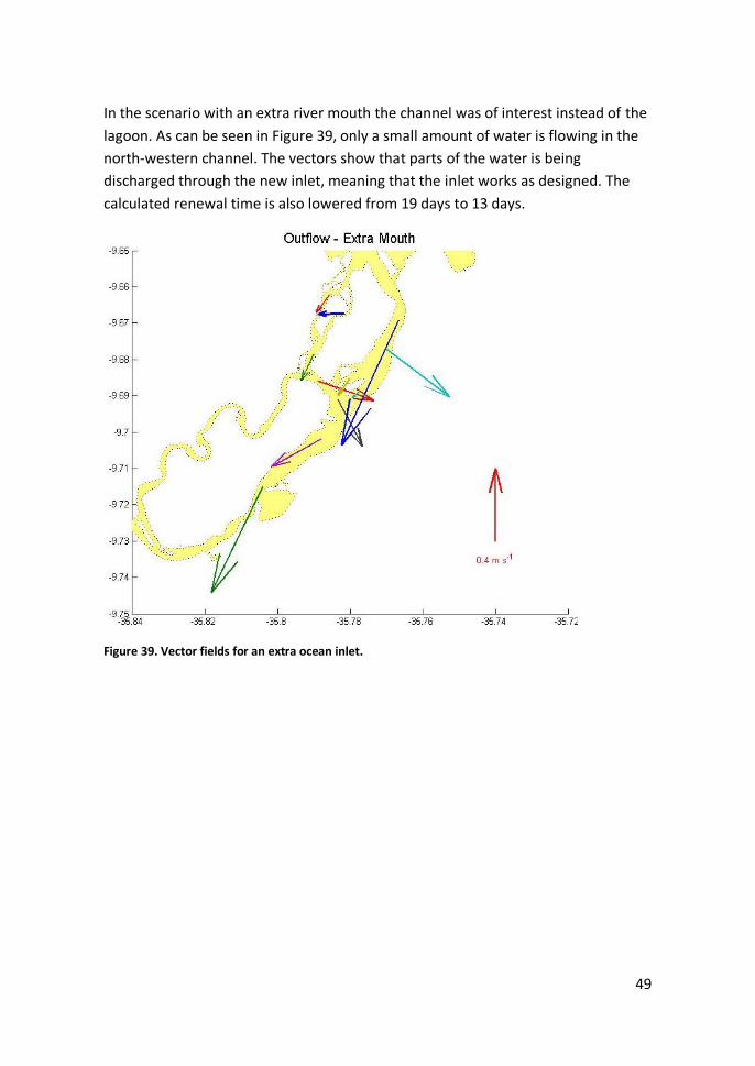
In the scenario with an extra river mouth the channel was of interest instead of the

lagoon. As can be seen in Figure 39, only a small amount of water is flowing in the

north-western channel. The vectors show that parts of the water is being

discharged through the new inlet, meaning that the inlet works as designed. The

calculated renewal time is also lowered from 19 days to 13 days.

Figure 39. Vector fields for an extra ocean inlet.

50

51

7 Discussion The expanding city of Maceio has experienced a deteriorating water quality in the

MMELS over the last decades. Several surveys have been carried out since the

1980s to get a better understanding of the lagoon system. All this information can

be utilized with IPH-ECO to make predictions about how the lagoon system will

react to future conditions such as high floods or sediment infilling at the ocean

inlet. It can also be used to simulate algae blooms, sediment transport and

dissolved oxygen, amongst others. The first step, however, is to calibrate the model

hydrodynamically.

7.1 Calibration Information about bottom sediments and bathymetry in Mundaú is extensive. As a

consequence, the process of calibrating Mundaú lagoon was fairly straightforward.

An adjustment of the friction coefficient in the channel and in the lagoon to match

the tidal range of the sensor and model was all that was required to obtain a good

match.

For Manguaba, however, only bathymetry data for the upper half of the lagoon is

known and information about sediments is scarce. Therefore Manguaba was more

difficult to calibrate. Numerous different parameter set-ups where tried to get the

best possible match. The southern part of the lagoon with the missing bathymetry

was modeled with water depths between one and three meters. The average

depth in the lagoon is 2.1 m and it seemed unrealistic to exceed this range in

depth. Numerous different Chezy coefficients were also incorporated but had little

effect on the tidal range in the lagoon. The channel leading into Manguaba is very

narrow, and acts as a bottleneck for the inflowing water. This part was also

modeled with various depths to allow more water to enter the lagoon, but without

success.

A good match between model and sensor was not achieved during the calibration

process. The inadequate information about Manguaba lagoon’s boundary

conditions is considered to be the reason why it was not successfully calibrated.

The small tidal range can also be a contributing factor. A difference of just a few

centimeters between the model and the sensor gives a high percentage of error.

Due to time constraints within the project, Manguaba could not be calibrated

further.

The model cannot represent the neap tide during 23rd of February in either of the

lagoons very well. During this neap tide the sensors shows a drop in the mean

52

water level. This general drop in water level is not as large in the model as

according to the sensor readings, which gives a low correlation between model and

sensor during this time. This is a phenomenon that is not easily explained. The

reluctance in the model to drop the general water level during a neap tide suggests

that friction is set too high in the channel. However, if the friction in the channel

leading to Mundaú is lowered, the tidal range in the lagoon will be too high.

In Manguaba lagoon the Chezy coefficient is set to 53, which is the lowest

acceptable friction according to the calculations with Cowan´s method. The channel

has a friction coefficient of 40, which can also be considered to be a high value for a

channel. The bad resemblance during neap tide in Manguaba is not explained by

too high friction. Here it is suspected that the lack of bathymetry values makes the

model present the lagoon with too shallow depths.

7.2 Estimation of Correlation To estimate the correlation between model and sensor, more than one statistical

parameter needed to be calculated in order to assess the correlation. The Pearson

correlation coefficient was almost 100 % in both lagoons, which proved that the

tidal phases were well synchronized. The RMS gives a mean value between

measured data and modeled. Manguaba presents a lower RMS than Mundaú, but

related to the tidal range, Manguaba’s RMS is proportionally larger than the one of

Mundaú. Mean tidal range comparison shows the difference in amplitude between

model and sensor, but does not show differences in lateral displacements. The

correlation diagram gives a good visual presentation of how the correlation

changes throughout the modeled period.

How large of an error that is acceptable in a model is not easily quantified. It has to

be put in relation to the precision needed for the application. In this case, Mundaú

was considered within the margin of error. The tidal range matched well

throughout the time period and the deviation during neap tide was not as great as

Manguaba. For Manguaba, neither tidal range nor depth variance matched

particularly well.

7.3 Renewal Time The renewal time was calculated using both IPH-ECO and sensor readings. By

comparing these two methods it can be seen that the one using sensor readings

does not satisfactorily match IPH-ECO when it comes to t50%, but gives a reasonably

good match for t99%. Depending on the purpose of the study it could be enough to

53

only use the sensor readings to save time. It is however impossible to make future

predictions with this method.

Oliviera and Kjerfve (1993) states that the retention time for Mundaú and

Manguaba is 16 days and 36 days respectively. There is no information about how

these numbers were conceived, but an average between retention time during dry-

and wet season is plausible to believe. It is also unknown if they have assumed

complete mixing or not. IPH-ECO states that the renewal times are 19 days and 42

days for Mundaú and Manguaba respectively during the dry season. Renewal times

during wet season would be lower than this, and it is believed that a calculated

average between wet- and dry season would come close to the estimation of

Oliviera and Kjerfve’s (1993) values.

7.4 Scenarios To prove the usability of the model it was tested with two plausible scenarios;

water level rise during high inflow from the Mundaú River, and the predicted

change of renewal time if a second ocean inlet was constructed in the vicinity of

the lagoon.

The data used for the high river inflow was from a significant runoff event in August

2011. Given climate change, other even higher values could be used to simulate a

worst case scenario. The high inflow scenario showed a water level rise from 0.5 m

to 2.0 m. This information regarding water level rise in the lagoon combined with

elevation data for the surrounding land near the lagoon can forecast how much

land will be flooded during such an event. Also noticeably in this scenario is that

the tidal variance is close to non-existent during this period. This proves the fact

that the water is only flowing in one direction during this period, towards the

ocean. If the only inflow entering the lagoon is fresh water from the river, this will

reduce the salinity in the lagoon. If the model were calibrated for salinity this

reduction could be quantified.

It is a known fact that much of the lagoons´ marine life depends on a certain level

of salinity in order to sustain life. Heavy runoff events like this can cause nuisance

or even death to some species when the drop in salinity is too high. IPH-ECO can in

this sense help to model a “maximum inflow scenario”, to determine how much

fresh water the lagoon can receive and still be able to sustain marine life. A

prediction like this could be important if, for example, a dam were to be

constructed along the river to better control heavy runoff events.

54

The opening of a new channel towards the ocean proved to lower the renewal time

for Mundaú lagoon. With the original mouth the t99% was 19 days during a spring

tide. The corresponding value with the new channel was 13 days. A low renewal

time is important for the lagoon in the sense that more pollution is being

transported to the ocean instead of residing within the lagoon. Mundaú lagoon

receives BOD-rich water both from the sewage in Maceió and from the nearby

sugar cane plantations.

A low renewal time causes a buildup of BOD-levels and combined with solar

radiation, it catalysts the growth of phytoplankton. This will eventually lead to

oxygen depletion, killing of the aquatic fauna. A lower renewal time also helps

bringing oxygenated water from the ocean and to hinder the buildup of high BOD-

concentrations within the lagoon. An extra opening to the ocean means that

salinity levels in the lagoon will be closer to oceanic salinity levels and that the

lagoon will drain faster during a high inflow event. It also means that the water

velocity in the original mouth will be lower when the flow is divided between two

mouths. This might cause sediment infilling, and in the long term, cancel out the

positive effect on the renewal time that was initially observed.

7.5 Future Recommendations In this chapter recommendations for the future integration of an IPH-ECO model in

the MMELS will be given. The recommendations are based on the experiences

acquired during the calibration and operation of this model.

7.5.1 Field Campaign

One sensor should be placed outside the lagoons´ inlet, thus eliminating

the necessity of using tidal prediction software and applying the arbitrary

reduction of 10 %.

It would be useful to place more than one sensor in each lagoon. This

would give knowledge about the tidal progression within the lagoons and

provide more data to calibrate the model with.

The bathymetry survey in Manguaba needs to be updated to also include

the southern part of the lagoon.

A sediment survey in Manguaba would help estimating the Chezy

coefficient more accurately.

55

7.5.2 IPH-ECO

IPH-ECO is a specialist tool with a high learning curve. A graphical user

interface, like the one constructed for v.1.0 of the model, could make it

easier to work with.

More flexibility to construct output files manually would be a great

improvement. In the case of illustrating vector fields, an output file

containing only the needed information from all the cells would give a

faster work flow and more detailed information.

The calibration of IPH-ECO in the MMELS could with great advantage be

continued with the salinity data that was also collected during this field

campaign.

7.6 Sources of Error When using tidal predication software, tidal height needed to be read hourly.

WTides does not offer any export of tidal height meaning that the values needed to

be read manually and put into a separate document. It is possible that some values

could be misread during this process due to human error. However, the values

where plotted afterwards and all the values took on the shape of a sinusoidal

curve. It was later discovered that the program WXTide offers export options.

When the vector fields were plotted the coordinates needed to be read manually

from ArcMap, if some of the coordinates was misread this would mean that the

arrow in the vector-field would be in the wrong position. It was also up to the

authors of this thesis to arbitrary chose the location of the vectors. As an effect of

this, some places of interest might have gone unseen.

The sensors used in the field campaign use a constant when converting actual

conductivity to a salinity value. A constant can be used to relate conductivity and

salinity to one another, but this constant is dependent on which type of water it is

being placed in. Other ions can affect the result of the conductivity more than Na+

and Cl-, it is therefore good to know the whole chemical composition of the water

before applying a constant. Even though salinity is not dealt with in this thesis, it is

used by the sensor to calculate the density of the water, and can thereby relate a

pressure to a water depth. Consequently, there is a chance of some error regarding

the water depth monitored by the sensors.

56

57

8 Conclusions The aim of this master thesis was to renew the hydrodynamic model in the MMELS

and gain a deeper understanding about lagoons and their water quality issues. In

order to do so, bathymetry and sediment surveys have been digitized and

implemented in IPH-ECO. A new field campaign has been carried out, where depth

and salinity data were recorded. This data can also be used for future work with

IPH-ECO.

Mundaú lagoon has been calibrated well hydrodynamically, thus it is now possible

to simulate different scenarios using IPH-ECO. With some further calibration it is

likely that also Manguaba lagoon could be modeled successfully concerning

hydrodynamics. If the model also was to be calibrated regarding salinity it could be

used to evaluate more complex environmental issues concerning the whole

system.

58

59

Bibliography ANA, 2012. Levantamento Batimétrico na Lagoa Mundaú, Maceió: ANA.

Bahr, L., 2010. Lacoastpost - All Things Coastal. [Online]

Available at: http://lacoastpost.com/blog/?p=29031

[Accessed 21 03 2014].

Brisbane City Council, n.d. Subdivision and Development Guideline Technical

Documents. [Online]

Available at:

http://www.brisbane.qld.gov.au/sites/default/files/ncd_appendixc_part3.pdf

[Accessed 12 02 2014].

Fragoso Jr., C. R., van Nes, E. H., Janse, J. H. & Motta Marques, D. d., 2009. IPH-

TRIMD3D-PClake: A Three-Dimensional Complex Dynamic Model for Subtropical

Aquatic Ecosystems, Porto Alegre: Elsevier.

Fragoso Jr., R. C., 2014. Professor at Center of Technology, Federal University of

Alagoas, Brazil [Interview] (15 01 2014).

Google Maps, 2014. Maceió. [Online]

Available at: https://www.google.se/maps/place/Macei%C3%B3/@-9.6607878,-

35.8208341,12z/data=!4m2!3m1!1s0x70138f2941ebc55:0xd1630decf3a3513

[Accessed 26 05 2014].

Gosh, S., 1998. Tidal Hydraulic Engineering. [Online]

Available at:

http://books.google.com.br/books?id=iVl_eqLJUAcC&pg=PA3&dq=tidal+componen

ts&hl=sv&sa=X&ei=tmbyUr2OOpOtsATIuYCADQ&redir_esc=y#v=onepage&q=tidal

%20components&f=false

[Accessed 05 02 2014].

HidroWeb, 2013. HidroWeb - Sistema de Informacoes Hidrologicas. [Online]

Available at: http://hidroweb.ana.gov.br/

[Accessed 15 02 2013].

In-Situ Europe, 2014. In-Situ Europe. [Online]

Available at: http://www.in-situ-

europe.com/pages/product/WQ_Aqua_TROLL_200.asp

[Accessed 01 03 2014].

60

Junior, L. C. C. et al., 2012. Assessment of the Trophic Status of four Coastal Lagoons

and one Estuarine Delta, Eastern Brazil, Maceió: Springer Science Business Media.

King, B. M., Rosopa, P. J. & Minium, E. W., 2011. Statistical Reasoning in the

Behavioral Sciences, s.l.: RR Donelly.

Kjerfve, B., 1994. Coastal Lagoon Processes, Amsterdam, The Netherlands: Elsevier

Science B.V.

Kjerfve, B. & Magill, K., 1989. Geopraphic and Hydrodynimic Characteristics of

Shallow Coastal Lagoons, Amsterdam: Elsevier Science Publishers.

Lages, A. M. G. & Lopes, M. E. P. d. A., 2005. Eniromental-Ethnical Behavior - The

Vinhoto Issue in Alagoas - Brazil. [Online]

Available at: https://www.academia.edu/2942505/ENVIRONMENTAL-

ETHICAL_BEHAVIOR_-_THE_VINHOTO_ISSUE_IN_ALAGOAS-_BRAZIL

[Accessed 03 02 2014].

Linnersund, J. & Mårtensson, E., 2008. Hydrodynamic Modelling and Estimation of

Exchange Rates for Bardawil Lagoon, Egypt, Lund: Lund University.

McKee, D., 2007. In-Situ Inc.. [Online]

Available at: http://www.in-situ.com/force_download.php?file_id=424

[Accessed 01 03 2014].

Miller, J., Pietrafesa, L. & Smith, M., 1990. Principles of Hydraulic Management of

Coastal Lagoons for Aquaculture and Fisheries. [Online]

Available at: http://www.fao.org/docrep/003/t0369E/T0369E02.htm#ch2.1.1

[Accessed 06 02 2014].

NOAA, 2008. NOAA Ocean Service Education. [Online]

Available at:

http://oceanservice.noaa.gov/education/kits/tides/media/supp_tide07a.html

[Accessed 23 05 2014].

Oliveira, A. M. & Kjerfve, B., 1993. Enviromental Response of a Tropical Lagoon

System to Hydrological Variability: Mundaú-Manguaba, Brazil, South Carolina,

Colombia: Academic Press Limited.

61

Pereira, F. F. et al., 2013. Assesment of Numerical Schemes for Solving the

Advection-Diffusion Equation on Unstructured Grids: Case Study of the Guaiba

River, Brazil, Lund: Lund University.

Petrobras, 2011. Levantamento Batimétrico na Área da Lagoa Manguaba (AL),

Salvador: Petrobras.

Prefeitura Municipal de Marechal Deodoro, 2011. Moradores Destacam Trabalho

Preventino Realizado em Barra Nove. [Online]

Available at: http://www.marechaldeodoro.al.gov.br/noticias/moradores-

destacam-trabalho-preventivo-realizado-em-barra-nova/

[Accessed 30 01 2014].

Ricketts, E. F., Jack, C. & Hedgpeth, J. W., 1985. Between Pacific Tides. [Online]

Available at:

http://books.google.com.br/books?id=tUl5ESavtRIC&printsec=frontcover&dq=tide

s&hl=sv&sa=X&ei=Re3nUsbqEsqhkQe5uYDQBA&redir_esc=y#v=onepage&q=tides

&f=false

[Accessed 28 01 2014].

US Army Corps of Engineers, 1984. Shore Protection Manual. 4th ed. Washington,

The US: US Army Corps of Engineers.

62

63

Appendix I

Aqua Troll 200 The sensor used in this field campaign was the Aqua Troll 200. It measures

pressure, temperature and actual conductivity of the water. It is enclosed in an

outer shell made of titanium to prevent it from corroding and can easily be fitted

with copper wire to prevent crustaceans from attaching to it, thus fouling the

reading of the sensor. (McKee, 2007)

The cable connected to the sensor is installed so that the uppermost part of the

cable is above the water surface. The reason for this is that the cable is ventilated

and serves as counter pressure for the diaphragm that measures the pressure.

Hence, the pressure being measured is the relative pressure rather than absolute

pressure. (McKee, 2007)

Figure I. 1. Aqua Troll 200 (In-Situ Europe, 2014).

Actual conductivity is measured by sending alternating current between six

electrode enclosed in the body. The sensor itself determines the voltage needed

depending on the temperature in the water. Since both temperature and actual

conductivity is known the sensor automatically calculates the specific conductivity

using the standard method 2520B. (McKee, 2007)

Salinity is also calculated through actual conductivity using standard method

2520B. Although salinity itself is of highest interest to measure, it also serves the

purpose of density calibration for when the depth is being calculated using the

pressure. The water depth is calculated according to (McKee, 2007):

64

Density of the water is salinity and temperature dependent and calculated with the empirical equation (McKee, 2007):

ρ ρ ρ

It is also possible to change the specific gravity with and correction factor (CFg) depending on which latitude the measurement takes place. The calculation for this is as follows (McKee, 2007): ρ

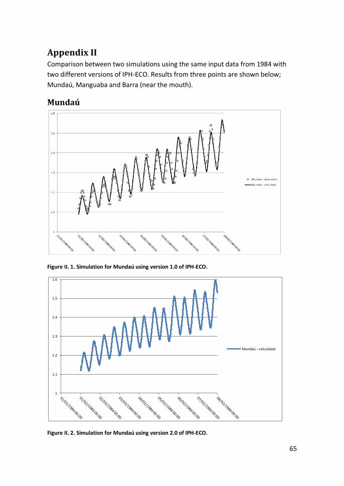
65

Appendix II Comparison between two simulations using the same input data from 1984 with

two different versions of IPH-ECO. Results from three points are shown below;

Mundaú, Manguaba and Barra (near the mouth).

Mundaú

Figure II. 1. Simulation for Mundaú using version 1.0 of IPH-ECO.

Figure II. 2. Simulation for Mundaú using version 2.0 of IPH-ECO.

1

1.1

1.2

1.3

1.4

1.5

1.6

Mundaú - calculated

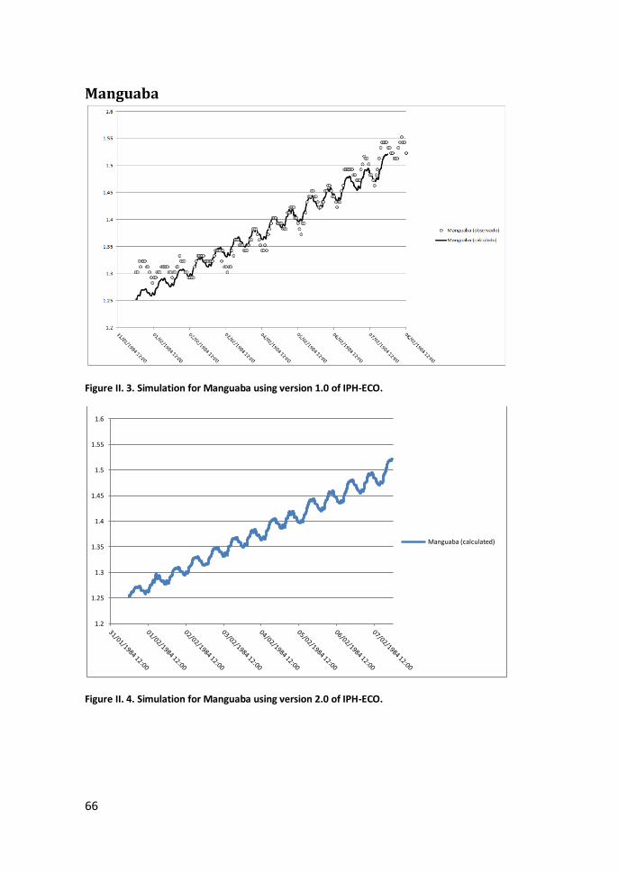
66

Manguaba

Figure II. 3. Simulation for Manguaba using version 1.0 of IPH-ECO.

Figure II. 4. Simulation for Manguaba using version 2.0 of IPH-ECO.

1.2

1.25

1.3

1.35

1.4

1.45

1.5

1.55

1.6

Manguaba (calculated)

67

Barra

Figure II. 5. Simulation for Barra using version 1.0 of IPH-ECO.

Figure II. 6. Simulation for Barra using version 2.0 of IPH-ECO.

0.7

0.9

1.1

1.3

1.5

1.7

1.9

2.1

2.3

Barra (calculated)

68

69

Appendix III The salinity data for both lagoons are presented below. As can be seen, the average

salinity level is higher in Mundaú than in Manguaba.

Figure III. 1. Salinity data for Mundaú.

Figure III. 2. Salinity data for Manguaba.

0

5

10

15

20

25

30

Salin

ity

(PSU

)

Mundaú

0

5

10

15

20

25

30

Salin

ity

(PSU

)

Manguaba

70

71

Appendix IV The combined flow of cell 207 and 586 in the channel leading to Mundaú is

summarized and presented in Figure IV. 1 and Figure IV. 2. During spring tide the

combined maximum flow is in the magnitude of 300 m3/s. During neap tide the

maximum flow is in the range of 150 m3/s.

Figure IV. 1. Combined flow 16 February.

Figure IV. 2 Combined flow 23 February.

-400

-300

-200

-100

0

100

200

300

400

Flo

w [

m3/s

]

Combined Flow 16 February

-400

-300

-200

-100

0

100

200

300

400

Flo

w [

m3/s

]

Combined Flow 23 February