HYDRODYNAMIC FORCES ACTING ON PIPE BENDS IN TWO-PHASE SLUG...
50
1 Statistical analysis of the hydrodynamic forces acting on pipe bends in gas-liquid slug flow and their relation to fatigue Boon Li Tay a, * , Rex B. Thorpe b a Department of Chemical Engineering, University of Cambridge, Pembroke Street, Cambridge CB2 3RA, UK. b Department of Chemical and Process Engineering, University of Surrey, Guildford GU2 7XH, UK. Abstract In this paper, the resultant hydrodynamic force ( R F , where 2 2 y x R F F F ) acting on pipe bends will be discussed. A hypothesis that the peak (resultant) forces, peak , R F acting on pipe bends can be described by the normal distribution function will be tested, with the purpose of predicting the mean of the peak , R F ( mean , R F ) and the standard deviations of the peak , R F ( deviation standard R, F ) generated. This in turn allows prediction of the probability of the largest forces that occasionally occur at various flow rates. This information is vital in designing an appropriate support for the piping system, to cater the maximum force over a long period of operation. Besides, this information is also important in selecting a pipe material or material for connections suitable to withstand fatigue failure, by reference to the S-N curves of materials. In many cases, large numbers of response cycles may accumulate over the life of the structure. By knowing the force distribution, ‘cumulative damage’ can also be determined; ‘cumulative damage’ is another phenomenon that can cause fatigue, apart from the reversal maximum force. Key Words: slug flow, bend, force, statistical analysis, fatigue, cumulative damage. * Corresponding author (email: [email protected])
Transcript of HYDRODYNAMIC FORCES ACTING ON PIPE BENDS IN TWO-PHASE SLUG...
1
Statistical analysis of the hydrodynamic forces
acting on pipe bends in gas-liquid slug flow and
their relation to fatigue
Boon Li Tay a, *, Rex B. Thorpe b
a Department of Chemical Engineering,
University of Cambridge,
Pembroke Street, Cambridge CB2 3RA, UK.
b Department of Chemical and Process Engineering,
University of Surrey,
Guildford GU2 7XH, UK.
Abstract
In this paper, the resultant hydrodynamic force ( RF , where 22
yxR FFF ) acting on
pipe bends will be discussed. A hypothesis that the peak (resultant) forces, peak,RF acting
on pipe bends can be described by the normal distribution function will be tested, with the
purpose of predicting the mean of the peak,RF ( mean,RF ) and the standard deviations of the
peak,RF ( deviation standard R,F ) generated. This in turn allows prediction of the probability of
the largest forces that occasionally occur at various flow rates. This information is vital in
designing an appropriate support for the piping system, to cater the maximum force over a
long period of operation. Besides, this information is also important in selecting a pipe
material or material for connections suitable to withstand fatigue failure, by reference to
the S-N curves of materials. In many cases, large numbers of response cycles may
accumulate over the life of the structure. By knowing the force distribution, ‘cumulative
damage’ can also be determined; ‘cumulative damage’ is another phenomenon that can
cause fatigue, apart from the reversal maximum force.
Key Words: slug flow, bend, force, statistical analysis, fatigue, cumulative damage.
* Corresponding author (email: [email protected])
2
1. Introduction
Slug flow is difficult to model in that slugs have varying lengths, densities, and
configurations; the forces acting on pipe bends or other pipe fittings vary with the slugs.
Distribution analysis of the resultant forces acting on pipe bends, due to the hydrodynamic
behaviour of slug flow, may be applied to serviceability checks and fatigue cycle
counting. This provides guidance to the designer whether or not the dynamics are of
importance i.e. not safely covered by fatigue load factors in conventional checks. A brief
summary of metal fatigue is attached in the Appendix.
Santana et al. (1993) reported that two-phase slug flow has been evident in the piping
systems at ARCO’s Kuparuk River Unit, North Slope, Alaska since shortly after startup in
1981. They further reported that the forces associated with slug flow had caused
excessive movement of partially restrained piping. Unrestrained elbows, tees and vessel
nozzles and internals were subject to deformation and cyclic stress. Eventually, the
magnitude and number of stress reversals caused fatigue cracking in piping branch
connections and a pressure vessel nozzle. They mentioned that research had been carried
out on the impacts of slug flow on their operating facilities. ARCO installed a data
acquisition system that records historic information such as the frequency of slugs and
accompanying stress reversals for a time period of a year or more, to provide an accurate
indication of the number and magnitude of stress reversal cycles experienced by piping,
vessel, and support structures. This will have allowed fatigue usage of the components of
ARCO’s modified design to be estimated, and it will also have been useful in predicting
the remaining fatigue life of the components. However, Santana et al. give no detail of
the data acquired.

3
The linear cumulative damage rule as defined by Miner (1945) is used in the majority of
fatigue life calculations. This rule assumes that if a bend has received 1n cycles at 1stress
for which the expected number of cycles to failure is 1N then a fraction 11 Nn of the
useful life is used up (Alexander & Brewer, 1963). The ‘cumulative damage’ is
calculated as:
i
i i
i
N
n
N
n
N
n
12
2
1
1
(1)
Failure will occur when 11
i
i i
i
N
n. A design value less than unity is generally used.
Cook and Claydon (1992) reported that tests have shown significant scatter and a marked
load order dependency and values of cumulative damage between 0.3 and 3 have been
obtained. Despite this load order dependency, there has been no physical basis supporting
the assumptions behind Miner (1945)’s rule; although this has widespread usage in
service life prediction in early stages of design. Cook & Claydon (1992) further
mentioned that in order to account for such a large scatter in fatigue test data and
variability in critical damage constant defined above, a factor of 1/5th or less is typically
used in design life calculations.
In addition, investigation showed the fatigue strength of un-welded pipe is twice of the
welded pipes, as a result of high stress concentration on the notch at the weld root
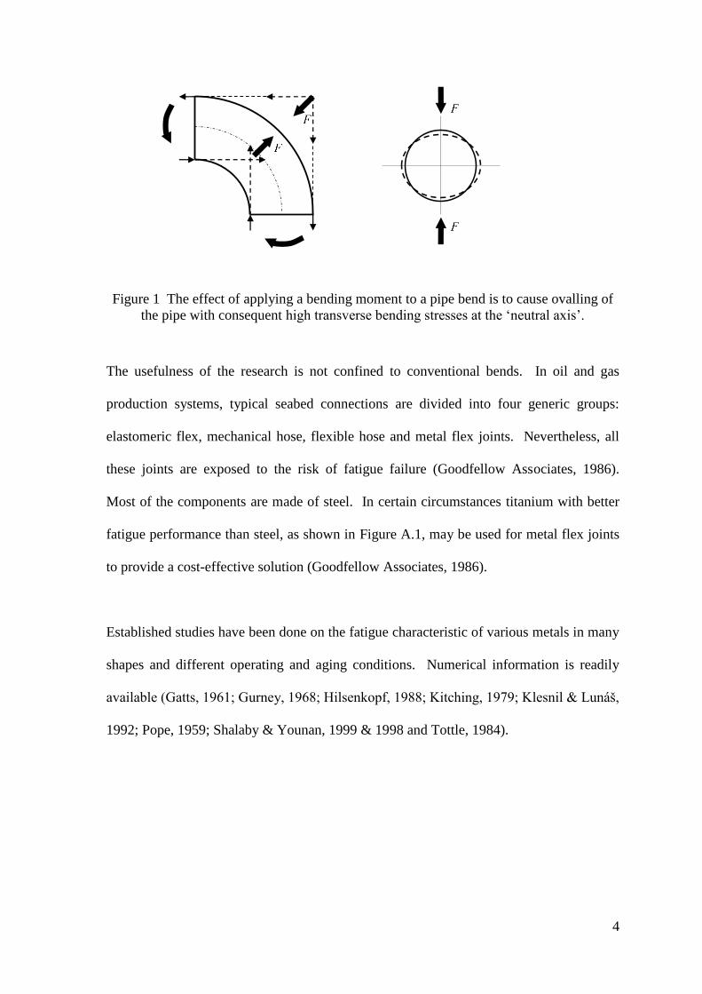
(Gurney, 1968). At a pipe bend there are higher stresses than exist in adjoining straight
runs of pipe (Gurney, 1968). Under an applied bending moment the cross-section of the
pipe tends to become oval, as shown in Figure 1. The fatigue strength of a bend will be a
function, by a factor less than unity, of the fatigue strength of the material.
4
Figure 1 The effect of applying a bending moment to a pipe bend is to cause ovalling of
the pipe with consequent high transverse bending stresses at the ‘neutral axis’.
The usefulness of the research is not confined to conventional bends. In oil and gas
production systems, typical seabed connections are divided into four generic groups:
elastomeric flex, mechanical hose, flexible hose and metal flex joints. Nevertheless, all
these joints are exposed to the risk of fatigue failure (Goodfellow Associates, 1986).
Most of the components are made of steel. In certain circumstances titanium with better
fatigue performance than steel, as shown in Figure A.1, may be used for metal flex joints
to provide a cost-effective solution (Goodfellow Associates, 1986).
Established studies have been done on the fatigue characteristic of various metals in many
shapes and different operating and aging conditions. Numerical information is readily
available (Gatts, 1961; Gurney, 1968; Hilsenkopf, 1988; Kitching, 1979; Klesnil & Lunáš,
1992; Pope, 1959; Shalaby & Younan, 1999 & 1998 and Tottle, 1984).
5
2. Experiment set-up
Force on pipe bends due to slug flow is an unsteady-state phenomenon. Therefore, it is
pertinent to obtain time varying measurements of the impact and some slug characteristics,
including slug velocity, liquid hold-up and pressure at the inlet and outlet of the bend that
contribute to this impact. It has been shown that isolating the bend from the upstream and
downstream pipe works is vital (Tay and Thorpe, 2002, 2004, 2014; Fairhurst, 1983;
Hargreaves and Slocombe, 1998). The experimental data discussed in this paper was
collected from the same experimental rig used by Tay & Thorpe (2002, 2004, 2014). A
short description of the experimental setup is given below.
The experimental rig was set up where air and water were mixed via a T-mixer and fed to
the flow system. The flow then ran through a 9 m horizontal run, where slug flow is
developed (naturally downstream of the T-mixer at certain gas and liquid velocities),
followed by a bend set-up (Figure 2) and a 3.0 m horizontal pipe, and finally discharged at
atmospheric pressure into an opened-top slug catcher. Water collected in the slug catcher
was returned to a water tank and re-circulated.
A o90 stainless steel bend of radius 105 mm and an internal diameter of 70 mm, which
gives a bend radius to pipe diameter ratio of 51.DR , was setup as shown in Figure 2.
Gaps of 3 mm were allowed between the bend and upstream and downstream pipe works,
to minimize structural transmission to and from the pipe bend, where force measurements
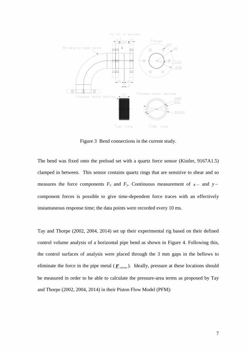
were taken. The gaps were closed from the external pipe wall using two sets of bellows,
see Figure 3. This setup reduced the disturbance on the main stream due to the sudden
increase and decrease in the flow area and eliminated the disturbance on the mainstream
due to the corrugated surface of the bellows (Tay and Thorpe, 2014).

6
Figure 2 Bend set-up.
7
Figure 3 Bend connections in the current study.
The bend was fixed onto the preload set with a quartz force sensor (Kistler, 9167A1.5)
clamped in between. This sensor contains quartz rings that are sensitive to shear and so
measures the force components Fx and Fy. Continuous measurement of x and y
component forces is possible to give time-dependent force traces with an effectively
instantaneous response time; the data points were recorded every 10 ms.
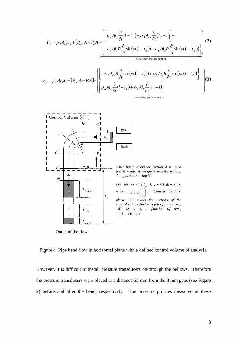
Tay and Thorpe (2002, 2004, 2014) set up their experimental rig based on their defined
control volume analysis of a horizontal pipe bend as shown in Figure 4. Following this,
the control surfaces of analysis were placed through the 3 mm gaps in the bellows to
eliminate the force in the pipe metal (stressF ). Ideally, pressure at these locations should
be measured in order to be able to calculate the pressure-area terms as proposed by Tay
and Thorpe (2002, 2004, 2014) in their Piston Flow Model (PFM):
8
momentum of change of rate
''
''
' ,
sinsin
bsBbsA
bsBasA
oaissAx
ttt
RAjttt
RAj
llt
Ajllt
Aj
APAPuAjF
(2)
momentum of change of rate
''
''
' ,
coscos
llt
Ajllt
Aj
ttt
RAjttt
RAj
APAPuAjF
esBdsA
bsBbsA
oeissBy
(3)
Figure 4 Pipe bend flow in horizontal plane with a defined control volume of analysis.
However, it is difficult to install pressure transducers on/through the bellows. Therefore
the pressure transducers were placed at a distance 55 mm from the 3 mm gaps (see Figure
2) before and after the bend, respectively. The pressure profiles measured at these
liquid
Control Volume
gas
us
us
Outlet of the flow
When liquid enters the section, A = liquid
and B = gas. When gas enters the section,
A = gas and B = liquid.
For the bend ( ),
where . Consider a fluid
phase “A” enters the sections of the
control volume that was full of fluid phase
“B” as is a function of time,
9
locations, after correction with a lag-time have been taken as the pressure profiles at the 3
mm gaps. Another pressure transducer was placed 1.5 m downstream after the bend.
Three conductance probes were located along the flow line, to provide information on
slug velocity, liquid hold-up and slug lengths. The conductance probes are made of two
parallel 0.125 mm stainless steel AISI 316L wires (Advent Research Materials Ltd,
FE632818) spaced 2 mm apart, passing vertically from the top to the bottom of the pipe.
Linear calibration relations were obtained between water level and output voltage. Tay
and Thorpe (2014) discussed the detailed setup of these conductance probes. The first two
probes were located 2.5 m (conductance probe 1) and 0.5 m (conductance probe 2) before
the bend, providing information on the slugs entering the bend. The other conductance
probe was placed 0.5 m after the bend, providing information on slugs leaving the bend.
Slug velocity ( su ) was obtained by dividing the distance between two conductance
probes, by the time taken for the liquid slug front to travel through these two points.
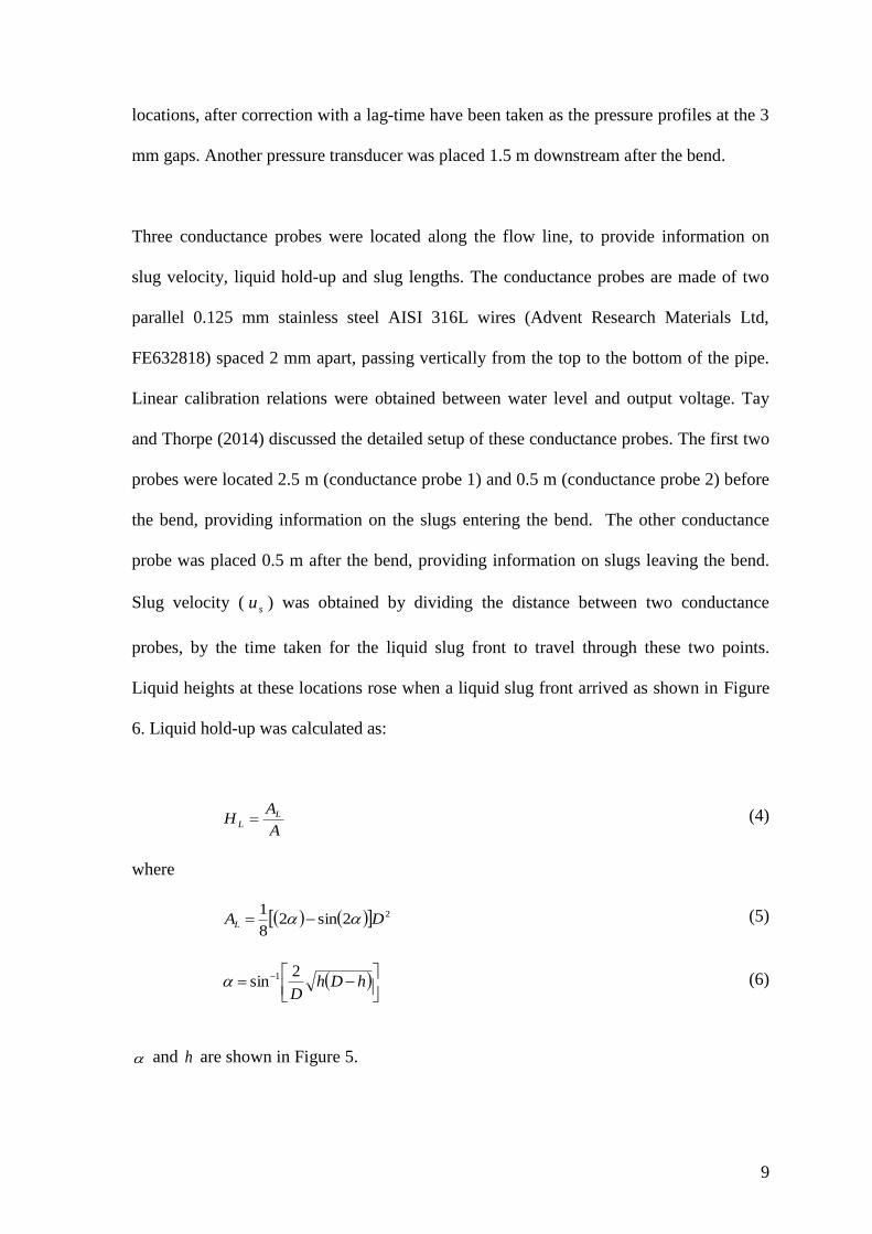
Liquid heights at these locations rose when a liquid slug front arrived as shown in Figure
6. Liquid hold-up was calculated as:
A
AH L
L (4)
where
22sin28
1DAL (5)
hDh
D
2sin 1 (6)
and h are shown in Figure 5.

10
Figure 5 Cross sectional view of pipe.
All the measuring devices were connected to a PC where the data were recorded using a
data acquisition program.
3. Experimental results: Statistical analysis of forces on pipe bend
3.1. Experimental force traces
A typical resultant force trace is given in Figure 6. The peak (resultant) force, peak,RF , is
the largest (resultant) force in the time-dependent resultant force trace imposed on the
pipe bend during transit of a slug unit. The maximum force, max,RF , is therefore referred
to the largest among the peak,RF s over a test period. In Figure 6, 3slugpeak,RF is the max,RF
over the 16 s measurement.
Wall of Perspex pipe
Liquid
Gas
Centre of the pipe
11
Figure 6 Traces of resultant force ( ) with liquid level ( ) in the pipe. (1-1 m.s81;m.s50 .j.j GL )
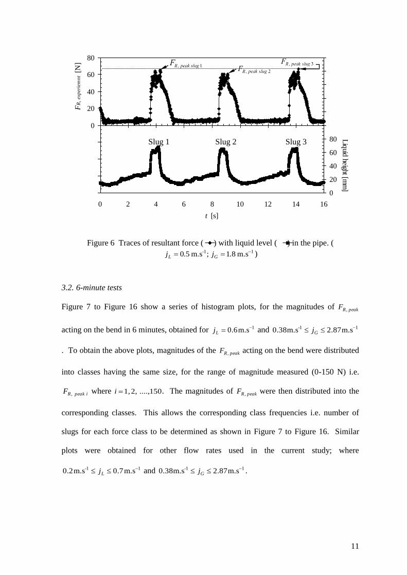
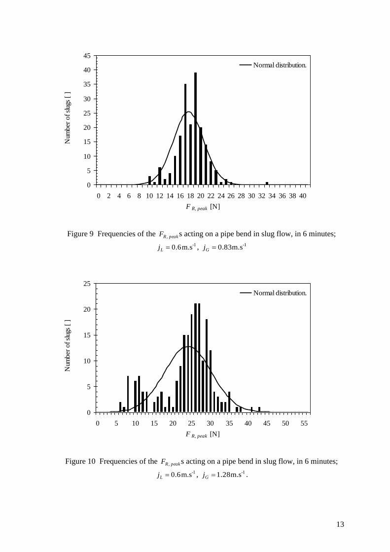
3.2. 6-minute tests
Figure 7 to Figure 16 show a series of histogram plots, for the magnitudes of peak,RF
acting on the bend in 6 minutes, obtained for 1m.s 0.6 Lj and 1-1 m.s 2.87m.s 0.38 Gj
. To obtain the above plots, magnitudes of the peak,RF acting on the bend were distributed
into classes having the same size, for the range of magnitude measured (0-150 N) i.e.
i peak,RF where 150 ...., 2, 1,i . The magnitudes of peak,RF were then distributed into the
corresponding classes. This allows the corresponding class frequencies i.e. number of
slugs for each force class to be determined as shown in Figure 7 to Figure 16. Similar
plots were obtained for other flow rates used in the current study; where
1-1 m.s 0.7m.s 0.2 Lj and 1-1 m.s 2.87m.s 0.38 Gj .
-80
-60
-40
-20
0
20
40
60
80
0 2 4 6 8 10 12 14 16
t [s]
FR
, ex
per
iem
nt [
N]
0
20
40
60
80
100
120
140
160
180
200L
iquid
height [mm
]
Slug 1 Slug 2 Slug 3

12
Figure 7 Frequencies of the peak,RF s acting on a pipe bend in slug flow, in 6 minutes;
-1m.s 0.6Lj , -1m.s 0.38Gj
Figure 8 Frequencies of the peak,RF s acting on a pipe bend in slug flow, in 6 minutes;
-1m.s 0.6Lj , -1m.s 0.60Gj
0
5
10
15
20
25
30
35
0 2 4 6 8 10 12 14 16 18 20 22 24 26 28 30
F R, peak [N]
Num
ber
of sl
ugs
[ ]
Normal distribution.
0
5
10
15
20
25
30
0 2 4 6 8 10 12 14 16 18 20 22 24 26 28 30
F R, peak [N]
Num
ber
of sl
ugs
[ ]
Normal distribution.
13
Figure 9 Frequencies of the peak,RF s acting on a pipe bend in slug flow, in 6 minutes;
-1m.s 0.6Lj , -1m.s 0.83Gj
Figure 10 Frequencies of the peak,RF s acting on a pipe bend in slug flow, in 6 minutes;
-1m.s 0.6Lj , -1m.s 1.28Gj .
0
5
10
15
20
25
30
35
40
45
0 2 4 6 8 10 12 14 16 18 20 22 24 26 28 30 32 34 36 38 40
F R, peak [N]
Num
ber
of sl
ugs
[ ]
Normal distribution.
0
5
10
15
20
25
0 5 10 15 20 25 30 35 40 45 50 55
F R, peak [N]
Num
ber
of sl
ugs
[ ]
Normal distribution.
14
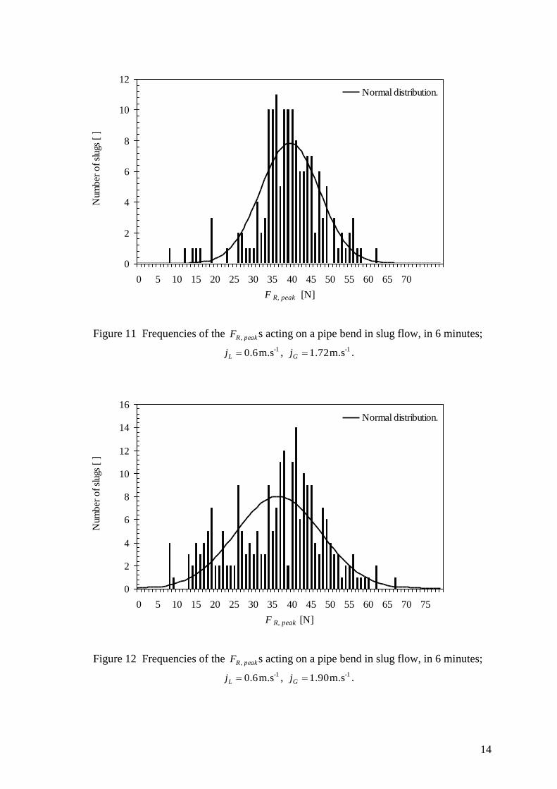
Figure 11 Frequencies of the peak,RF s acting on a pipe bend in slug flow, in 6 minutes;
-1m.s 0.6Lj , -1m.s 1.72Gj .
Figure 12 Frequencies of the peak,RF s acting on a pipe bend in slug flow, in 6 minutes;
-1m.s 0.6Lj , -1m.s 1.90Gj .
0
2
4
6
8
10
12
0 5 10 15 20 25 30 35 40 45 50 55 60 65 70
F R, peak [N]
Num
ber
of sl
ugs
[ ]
Normal distribution.
0
2
4
6
8
10
12
14
16
0 5 10 15 20 25 30 35 40 45 50 55 60 65 70 75
F R, peak [N]
Num
ber
of sl
ugs
[ ]
Normal distribution.
15
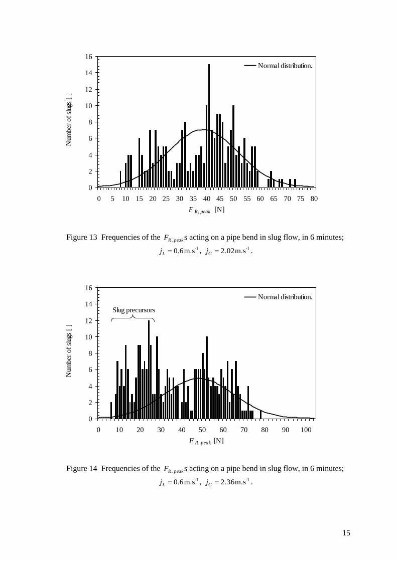
Figure 13 Frequencies of the peak,RF s acting on a pipe bend in slug flow, in 6 minutes;
-1m.s 0.6Lj , -1m.s 2.02Gj .
Figure 14 Frequencies of the peak,RF s acting on a pipe bend in slug flow, in 6 minutes;
-1m.s 0.6Lj , -1m.s 2.36Gj .
0
2
4
6
8
10
12
14
16
0 5 10 15 20 25 30 35 40 45 50 55 60 65 70 75 80
F R, peak [N]
Num
ber
of sl
ugs
[ ]
Normal distribution.
0
2
4
6
8
10
12
14
16
0 10 20 30 40 50 60 70 80 90 100
F R, peak [N]
Num
ber
of sl
ugs
[ ]
Normal distribution.
Slug precursors
16
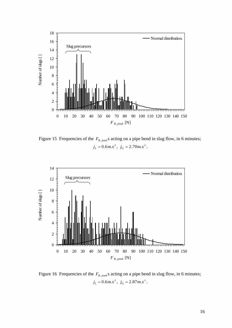
Figure 15 Frequencies of the peak,RF s acting on a pipe bend in slug flow, in 6 minutes;
-1m.s 0.6Lj , -1m.s 2.70Gj .
Figure 16 Frequencies of the peak,RF s acting on a pipe bend in slug flow, in 6 minutes;
-1m.s 0.6Lj , -1m.s 2.87Gj .
0
2
4
6
8
10
12
14
16
18
0 10 20 30 40 50 60 70 80 90 100 110 120 130 140 150
F R, peak [N]
Num
ber
of sl
ugs
[ ]
Normal distribution.
Slug precursors
0
2
4
6
8
10
12
14
0 10 20 30 40 50 60 70 80 90 100 110 120 130 140 150
F R, peak [N]
Num
ber
of sl
ugs
[ ]
Normal distribution.Slug precursors
17
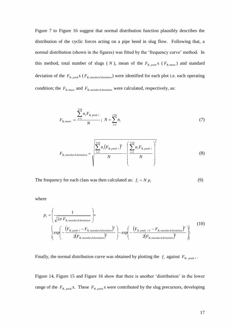
Figure 7 to Figure 16 suggest that normal distribution function plausibly describes the
distribution of the cyclic forces acting on a pipe bend in slug flow. Following that, a
normal distribution (shown in the figures) was fitted by the ‘frequency curve’ method. In
this method, total number of slugs ( N ), mean of the peak,RF s ( meanR,F ) and standard
deviation of the peak,RF s ( deviation standardR,F ) were identified for each plot i.e. each operating
condition; the meanR,F and deviation standardR,F were calculated, respectively, as:
N
Fn
F i
i peak R,i
meanR,
150
1 ;
150
1i
inN (7)
2
150
1
150
1
2
N
Fn
N
Fn
F i
i peak R,i
i
i peak R,i
deviation standardR, (8)
The frequency for each class was then calculated as: ii pNf (9)
where
2
2
1
2
2
2
2
2
1
deviation standardR,
deviation standardR,-ipeakR,
deviation standardR,
deviation standardR,ipeakR,
deviation standardR,
i
F
FFexp
F
FFexp
Fp
(10)
Finally, the normal distribution curve was obtained by plotting the if against i peak,RF .
Figure 14, Figure 15 and Figure 16 show that there is another ‘distribution’ in the lower
range of the peak,RF s. These peak,RF s were contributed by the slug precursors, developing
18
slugs arriving at the bend due to the relatively short upstream pipe available in the current
study (which was limited by the size of the laboratory). Neglecting the slug precursors,
the peak,RF s acting on pipe bends were found to be well described by normal distribution
function.
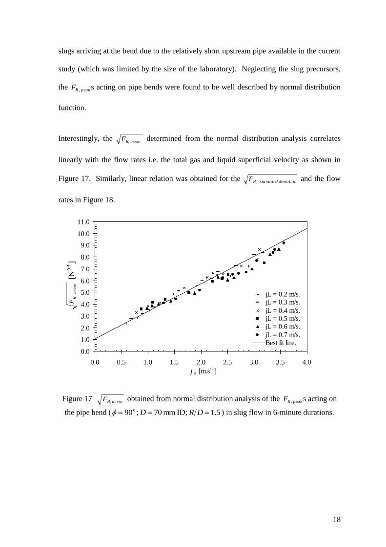
Interestingly, the meanR,F determined from the normal distribution analysis correlates
linearly with the flow rates i.e. the total gas and liquid superficial velocity as shown in
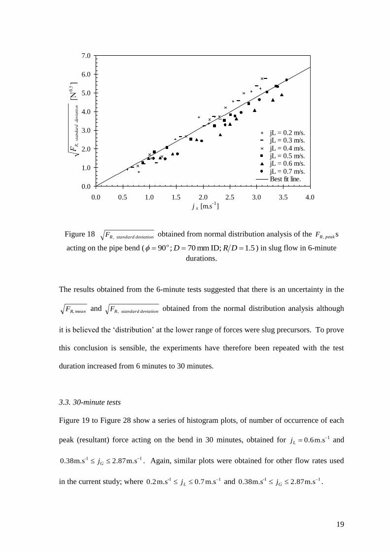
Figure 17. Similarly, linear relation was obtained for the deviationstandard,RF and the flow
rates in Figure 18.
Figure 17 meanR,F obtained from normal distribution analysis of the peak,RF s acting on
the pipe bend ( 5.1ID; mm 70 ;90o DRD ) in slug flow in 6-minute durations.
0.0
1.0
2.0
3.0
4.0
5.0
6.0
7.0
8.0
9.0
10.0
11.0
0.0 0.5 1.0 1.5 2.0 2.5 3.0 3.5 4.0
j s [m.s-1
]
jL = 0.2 m/s.jL = 0.3 m/s.
jL = 0.4 m/s.jL = 0.5 m/s.jL = 0.6 m/s.
jL = 0.7 m/s.Best fit line.
19
Figure 18 deviationstandard,RF obtained from normal distribution analysis of the peak,RF s
acting on the pipe bend ( 5.1ID; mm 70 ;90o DRD ) in slug flow in 6-minute
durations.
The results obtained from the 6-minute tests suggested that there is an uncertainty in the
meanR,F and deviationstandard,RF obtained from the normal distribution analysis although
it is believed the ‘distribution’ at the lower range of forces were slug precursors. To prove
this conclusion is sensible, the experiments have therefore been repeated with the test
duration increased from 6 minutes to 30 minutes.
3.3. 30-minute tests
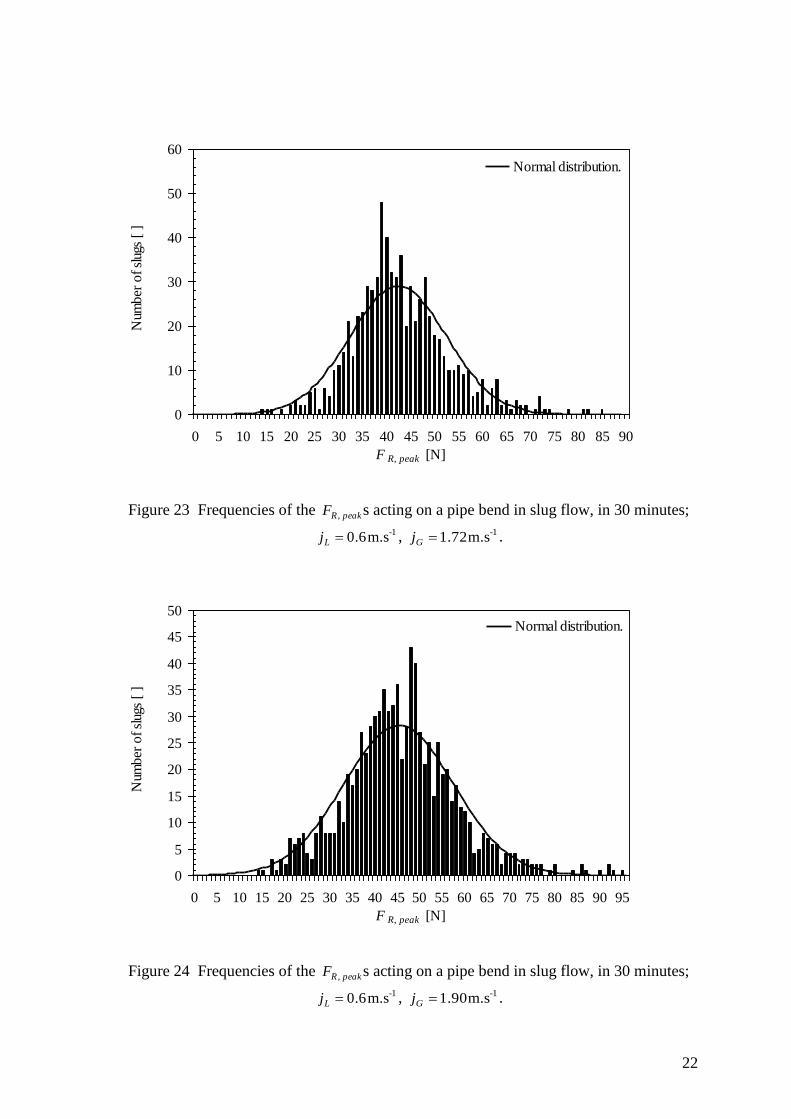
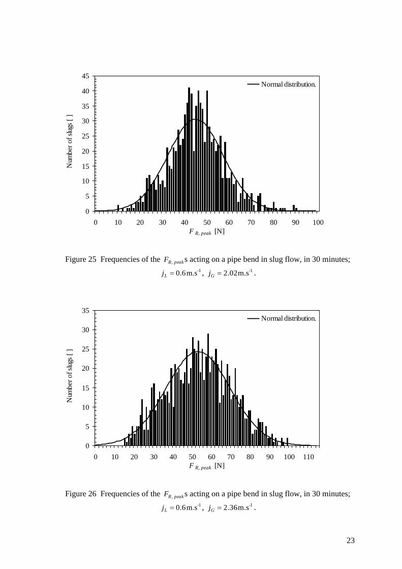
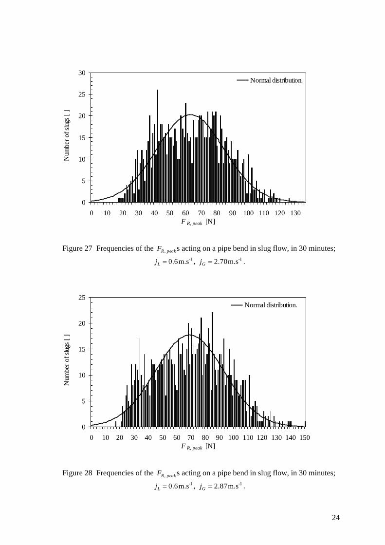
Figure 19 to Figure 28 show a series of histogram plots, of number of occurrence of each
peak (resultant) force acting on the bend in 30 minutes, obtained for 1m.s 0.6 Lj and
1-1 m.s 2.87m.s 0.38 Gj . Again, similar plots were obtained for other flow rates used
in the current study; where 1-1 m.s 0.7m.s 0.2 Lj and 1-1 m.s 2.87m.s 0.38 Gj .
0.0
1.0
2.0
3.0
4.0
5.0
6.0
7.0
0.0 0.5 1.0 1.5 2.0 2.5 3.0 3.5 4.0
j s [m.s-1
]
jL = 0.2 m/s.jL = 0.3 m/s.jL = 0.4 m/s.jL = 0.5 m/s.jL = 0.6 m/s.jL = 0.7 m/s.Best fit line.
20
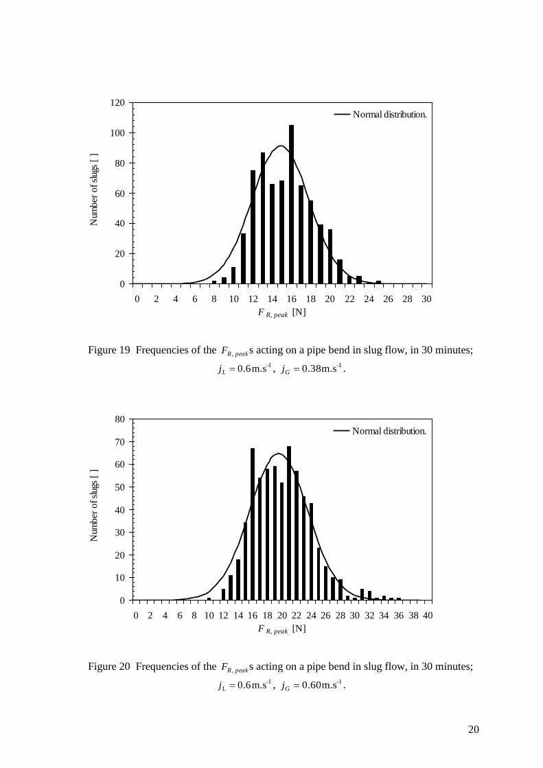
Figure 19 Frequencies of the peak,RF s acting on a pipe bend in slug flow, in 30 minutes;
-1m.s 0.6Lj , -1m.s 0.38Gj .
Figure 20 Frequencies of the peak,RF s acting on a pipe bend in slug flow, in 30 minutes;
-1m.s 0.6Lj , -1m.s 0.60Gj .
0
20
40
60
80
100
120
0 2 4 6 8 10 12 14 16 18 20 22 24 26 28 30
F R, peak [N]
Num
ber
of sl
ugs
[ ]
Normal distribution.
0
10
20
30
40
50
60
70
80
0 2 4 6 8 10 12 14 16 18 20 22 24 26 28 30 32 34 36 38 40
F R, peak [N]
Num
ber
of sl
ugs
[ ]
Normal distribution.

21
Figure 21 Frequencies of the peak,RF s acting on a pipe bend in slug flow, in 30 minutes;
-1m.s 0.6Lj , -1m.s 0.83Gj .
Figure 22 Frequencies of the peak,RF s acting on a pipe bend in slug flow, in 30 minutes;
-1m.s 0.6Lj , -1m.s 1.28Gj .
0
20
40
60
80
100
120
0 2 4 6 8 10 12 14 16 18 20 22 24 26 28 30 32 34 36 38 40 42 44 46
F R, peak [N]
Num
ber
of sl
ugs
[ ]
Normal distribution.
0
10
20
30
40
50
60
70
80
90
0 5 10 15 20 25 30 35 40 45 50 55 60
F R, peak [N]
Num
ber
of sl
ugs
[ ]
Normal distribution.
22
Figure 23 Frequencies of the peak,RF s acting on a pipe bend in slug flow, in 30 minutes;
-1m.s 0.6Lj , -1m.s 1.72Gj .
Figure 24 Frequencies of the peak,RF s acting on a pipe bend in slug flow, in 30 minutes;
-1m.s 0.6Lj , -1m.s 1.90Gj .
0
10
20
30
40
50
60
0 5 10 15 20 25 30 35 40 45 50 55 60 65 70 75 80 85 90
F R, peak [N]
Num
ber
of sl
ugs
[ ]
Normal distribution.
0
5
10
15
20
25
30
35
40
45
50
0 5 10 15 20 25 30 35 40 45 50 55 60 65 70 75 80 85 90 95
F R, peak [N]
Num
ber
of sl
ugs
[ ]
Normal distribution.
23
Figure 25 Frequencies of the peak,RF s acting on a pipe bend in slug flow, in 30 minutes;
-1m.s 0.6Lj , -1m.s 2.02Gj .
Figure 26 Frequencies of the peak,RF s acting on a pipe bend in slug flow, in 30 minutes;
-1m.s 0.6Lj , -1m.s 2.36Gj .
0
5
10
15
20
25
30
35
40
45
0 10 20 30 40 50 60 70 80 90 100
F R, peak [N]
Num
ber
of sl
ugs
[ ]
Normal distribution.
0
5
10
15
20
25
30
35
0 10 20 30 40 50 60 70 80 90 100 110
F R, peak [N]
Num
ber
of sl
ugs
[ ]
Normal distribution.
24
Figure 27 Frequencies of the peak,RF s acting on a pipe bend in slug flow, in 30 minutes;
-1m.s 0.6Lj , -1m.s 2.70Gj .
Figure 28 Frequencies of the peak,RF s acting on a pipe bend in slug flow, in 30 minutes;
-1m.s 0.6Lj , -1m.s 2.87Gj .
0
5
10
15
20
25
30
0 10 20 30 40 50 60 70 80 90 100 110 120 130
F R, peak [N]
Num
ber
of sl
ugs
[ ]
Normal distribution.
0
5
10
15
20
25
0 10 20 30 40 50 60 70 80 90 100 110 120 130 140 150
F R, peak [N]
Num
ber
of sl
ugs
[ ]
Normal distribution.

25
Figure 19 to Figure 28 with 5 times the sample size in 6-minute tests, confirmed the
earlier findings that (1) normal distribution function plausibly describes the distribution of
the cyclic force acting on a pipe bend in slug flow, (2) the ‘distributions’ in the lower
range of the peakR,F s in Figure 14, Figure 15 and Figure 16 were contributed by the slug
precursors. Again, the meanR,F determined from the normal distribution analysis on
peakR,F s obtained from the 30-minute tests, and the corresponding deviationstandard,RF
correlates linearly with the flow rates. Besides that, meanR,F and deviationstandard,RF
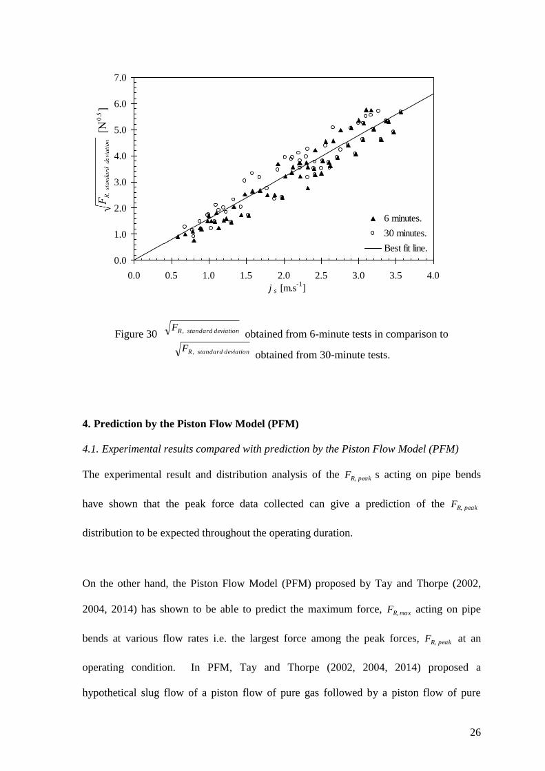
obtained from the 6-minute tests agree with the results from the 30-minute tests. This is
shown in Figure 29 and Figure 30.
Figure 29 meanR,F obtained from 6-minute tests in comparison to meanR,F obtained
from 30-minute tests.
0.0
2.0
4.0
6.0
8.0
10.0
12.0
0.0 0.5 1.0 1.5 2.0 2.5 3.0 3.5 4.0
j s [m.s-1
]
6 minutes.
30 minutes.
Best fit line.
26
Figure 30 deviationstandard,RF obtained from 6-minute tests in comparison to
deviationstandard,RF obtained from 30-minute tests.
4. Prediction by the Piston Flow Model (PFM)
4.1. Experimental results compared with prediction by the Piston Flow Model (PFM)
The experimental result and distribution analysis of the peakR,F s acting on pipe bends
have shown that the peak force data collected can give a prediction of the peakR,F
distribution to be expected throughout the operating duration.
On the other hand, the Piston Flow Model (PFM) proposed by Tay and Thorpe (2002,
2004, 2014) has shown to be able to predict the maximum force, maxR,F acting on pipe
bends at various flow rates i.e. the largest force among the peak forces, peakR,F at an
operating condition. In PFM, Tay and Thorpe (2002, 2004, 2014) proposed a
hypothetical slug flow of a piston flow of pure gas followed by a piston flow of pure
0.0
1.0
2.0
3.0
4.0
5.0
6.0
7.0
0.0 0.5 1.0 1.5 2.0 2.5 3.0 3.5 4.0
j s [m.s-1
]
6 minutes.
30 minutes.
Best fit line.
27
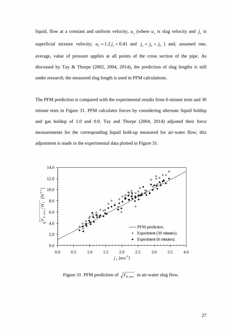
liquid, flow at a constant and uniform velocity, su (where su is slug velocity and sj is
superficial mixture velocity; 41.02.1 ss ju and GLs jjj ) and, assumed one,
average, value of pressure applies at all points of the cross section of the pipe. As
discussed by Tay & Thorpe (2002, 2004, 2014), the prediction of slug lengths is still
under research; the measured slug length is used in PFM calculations.
The PFM prediction is compared with the experimental results from 6-minute tests and 30
minute tests in Figure 31. PFM calculates forces by considering alternate liquid holdup
and gas holdup of 1.0 and 0.0. Tay and Thorpe (2004, 2014) adjusted their force
measurements for the corresponding liquid hold-up measured for air-water flow; this
adjustment is made in the experimental data plotted in Figure 31.
Figure 31 PFM prediction of max,RF in air-water slug flow.
0.0
2.0
4.0
6.0
8.0
10.0
12.0
14.0
0.0 0.5 1.0 1.5 2.0 2.5 3.0 3.5 4.0
j s [m.s-1
]
PFM prediction.
Experiment (30 minutes).
Experiment (6 minutes).
28
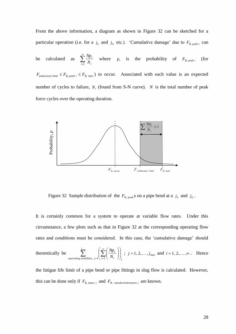
From the above information, a diagram as shown in Figure 32 can be sketched for a
particular operation (i.e. for a Lj and Gj etc.). ‘Cumulative damage’ due to i peakR,F can
be calculated as
1i i
i
N
Np where ip is the probability of i peakR,F (for
max R,i peakR,limit endurance FFF ) to occur. Associated with each value is an expected
number of cycles to failure, iN (found from S-N curve). N is the total number of peak
force cycles over the operating duration.
Figure 32 Sample distribution of the peak,RF s on a pipe bend at a Lj and Gj .
It is certainly common for a system to operate at variable flow rates. Under this
circumstance, a few plots such as that in Figure 32 at the corresponding operating flow
rates and conditions must be considered. In this case, the ‘cumulative damage’ should
theoretically be
maxj
jcondition, operating ji i
i
N
Np
1 1
; maxj,j 2,1, and ,i 2,1, . Hence
the fatigue life limit of a pipe bend or pipe fittings in slug flow is calculated. However,
this can be done only if j mean R,F and j deviationstandard,RF are known.
Pro
bab
ilit
y, p
29
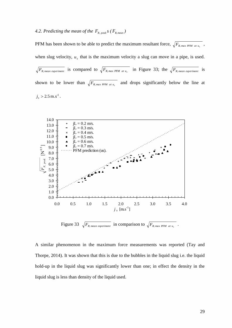
4.2. Predicting the mean of the peakRF , s ( meanR,F )
PFM has been shown to be able to predict the maximum resultant force, u at PFM maxR, sF ,
when slug velocity, su that is the maximum velocity a slug can move in a pipe, is used.
experiment meanR,F is compared to u at PFM maxR, sF in Figure 33; the experiment meanR,F is
shown to be lower than u at PFM maxR, sF and drops significantly below the line at
-1m.s 52.js .
Figure 33 experiment meanR,F in comparison to u at PFM maxR, sF .
A similar phenomenon in the maximum force measurements was reported (Tay and
Thorpe, 2014). It was shown that this is due to the bubbles in the liquid slug i.e. the liquid
hold-up in the liquid slug was significantly lower than one; in effect the density in the
liquid slug is less than density of the liquid used.
0.0
1.0
2.0
3.0
4.0
5.0
6.0
7.0
8.0
9.0
10.0
11.0
12.0
13.0
14.0
0.0 0.5 1.0 1.5 2.0 2.5 3.0 3.5 4.0
j s [m.s-1
]
jL = 0.2 m/s.jL = 0.3 m/s.jL = 0.4 m/s.jL = 0.5 m/s.jL = 0.6 m/s.jL = 0.7 m/s.PFM prediction (us).

30
As discussed, Tay and Thorpe (2004, 2014) adjusted their force measurements for the
corresponding liquid hold-up measured for air-water flow and this adjustment brought the
force measurements back to the PFM line. Following the same method, the measured
liquid hold-up (Figure 34) is used to adjust the force measurements by plotting
LmeanR, HF against sj as shown in Figure 35. Figure 35 shows that the data,
Lexperiment meanR, HF is lower than u at PFM maxR, sF but close to it. Therefore, it is thought
that the LmeanR, HF may plausibly be predicted by PFM, by considering slugs flow
down the pipe at the total superficial velocity, sj . Therefore, PFM has been used to
predict the force that a slug can exert on the pipe bend, sj at PFMR,F , when it moves at the
total superficial velocity (𝑗𝑠). The Lexperiment meanR, HF is compared to sj at PFMR,F and
u at PFM maxR, sF in Figure 35. Figure 35 shows that Lexperiment meanR, HF falls between
sj at PFMR,F and u at PFM maxR, sF .
0.0
0.2
0.4
0.6
0.8
1.0
1.2
0.0 0.5 1.0 1.5 2.0 2.5 3.0 3.5 4.0
j s [m.s-1
]
HL
[ ]
Current study.
Gregory (1978).
Malnes (1982).
31
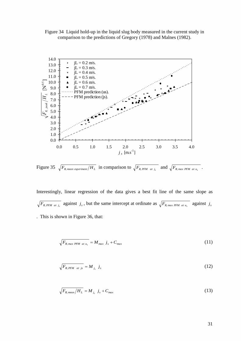
Figure 34 Liquid hold-up in the liquid slug body measured in the current study in
comparison to the predictions of Gregory (1978) and Malnes (1982).
Figure 35 Lexperiment meanR, HF in comparison to j at PFMR, sF and u at PFM maxR, s
F .
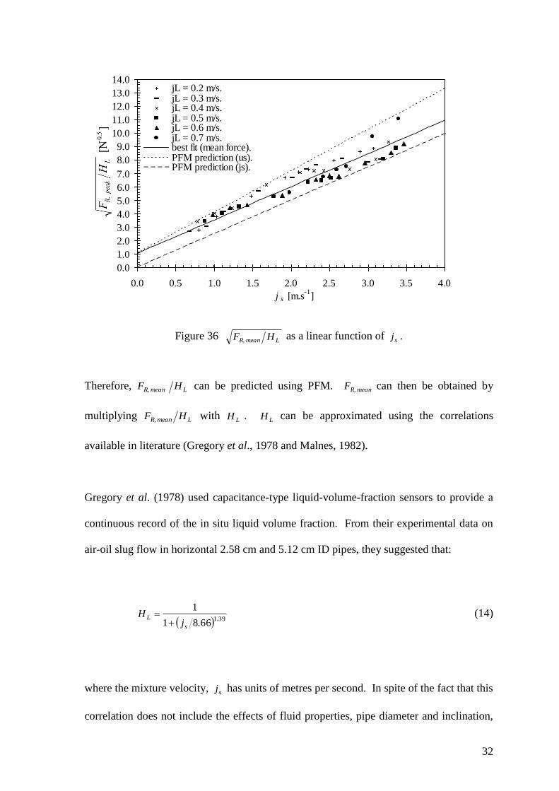
Interestingly, linear regression of the data gives a best fit line of the same slope as
sj at PFMR,F against sj , but the same intercept at ordinate as u at PFM maxR, sF against sj
. This is shown in Figure 36, that:
maxsmaxu at PFM maxR, CjMFs
(11)
sjjs at PFMR, jMFs
(12)
maxsjLmeanR, CjMHFs
(13)
0.0
1.0
2.0
3.0
4.0
5.0
6.0
7.0
8.0
9.0
10.0
11.0
12.0
13.0
14.0
0.0 0.5 1.0 1.5 2.0 2.5 3.0 3.5 4.0
j s [m.s-1
]
jL = 0.2 m/s.jL = 0.3 m/s.jL = 0.4 m/s.jL = 0.5 m/s.jL = 0.6 m/s.jL = 0.7 m/s.PFM prediction (us).PFM prediction (js).
32
Figure 36 LmeanR, HF as a linear function of sj .
Therefore, LmeanR, HF can be predicted using PFM. meanR,F can then be obtained by
multiplying LmeanR, HF with LH . LH can be approximated using the correlations
available in literature (Gregory et al., 1978 and Malnes, 1982).
Gregory et al. (1978) used capacitance-type liquid-volume-fraction sensors to provide a
continuous record of the in situ liquid volume fraction. From their experimental data on
air-oil slug flow in horizontal 2.58 cm and 5.12 cm ID pipes, they suggested that:
3916681
1.
s
L.j
H
(14)
where the mixture velocity, sj has units of metres per second. In spite of the fact that this
correlation does not include the effects of fluid properties, pipe diameter and inclination,
0.0
1.0
2.0
3.0
4.0
5.0
6.0
7.0
8.0
9.0
10.0
11.0
12.0
13.0
14.0
0.0 0.5 1.0 1.5 2.0 2.5 3.0 3.5 4.0
j s [m.s-1
]
jL = 0.2 m/s.jL = 0.3 m/s.jL = 0.4 m/s.jL = 0.5 m/s.jL = 0.6 m/s.jL = 0.7 m/s.best fit (mean force).PFM prediction (us).PFM prediction (js).
33
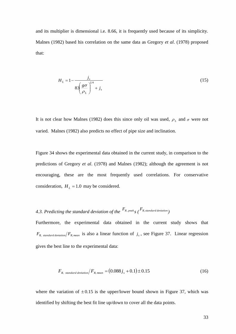
and its multiplier is dimensional i.e. 8.66, it is frequently used because of its simplicity.
Malnes (1982) based his correlation on the same data as Gregory et al. (1978) proposed
that:
s
L
sL
jg
jH
41
83
1
(15)
It is not clear how Malnes (1982) does this since only oil was used, L and were not
varied. Malnes (1982) also predicts no effect of pipe size and inclination.
Figure 34 shows the experimental data obtained in the current study, in comparison to the
predictions of Gregory et al. (1978) and Malnes (1982); although the agreement is not
encouraging, these are the most frequently used correlations. For conservative
consideration, 0.1LH may be considered.
4.3. Predicting the standard deviation of the peak,RFs ( deviation standardR,F
)
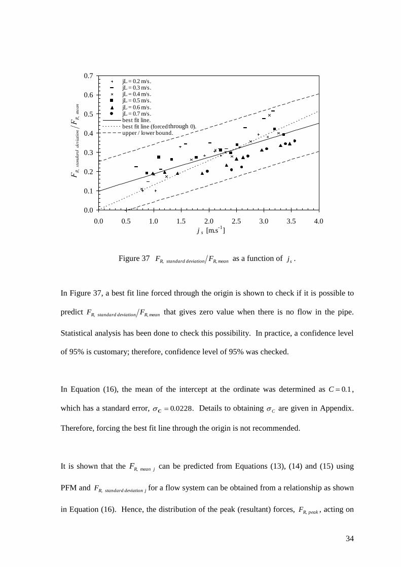
Furthermore, the experimental data obtained in the current study shows that
meanR,deviation standardR, FF is also a linear function of sj , see Figure 37. Linear regression
gives the best line to the experimental data:
15.01.0088.0 smeanR,deviation standardR, jFF (16)
where the variation of 15.0 is the upper/lower bound shown in Figure 37, which was
identified by shifting the best fit line up/down to cover all the data points.
34
Figure 37 meanR,deviation standardR, FF as a function of sj .
In Figure 37, a best fit line forced through the origin is shown to check if it is possible to
predict meanR,deviation standardR, FF that gives zero value when there is no flow in the pipe.
Statistical analysis has been done to check this possibility. In practice, a confidence level
of 95% is customary; therefore, confidence level of 95% was checked.
In Equation (16), the mean of the intercept at the ordinate was determined as 10.C ,
which has a standard error, 02280.C . Details to obtaining C are given in Appendix.
Therefore, forcing the best fit line through the origin is not recommended.
It is shown that the j eanmR,F can be predicted from Equations (13), (14) and (15) using
PFM and j deviation standardR,F for a flow system can be obtained from a relationship as shown
in Equation (16). Hence, the distribution of the peak (resultant) forces, peakR,F , acting on
0.0
0.1
0.2
0.3
0.4
0.5
0.6
0.7
0.0 0.5 1.0 1.5 2.0 2.5 3.0 3.5 4.0
j s [m.s-1
]
jL = 0.2 m/s.jL = 0.3 m/s.jL = 0.4 m/s.jL = 0.5 m/s.
jL = 0.6 m/s.jL = 0.7 m/s.best fit line.best fit line (forced thruogh 0).upper / lower bound.
through
35
a pipe bend for an operating condition can be obtained. With this, the fatigue life limit of
a pipe bend or pipe fittings in slug flow can be calculated. An example is given in
Appendix for estimating the fatigue life of the bend used in the current study, based on
statistical data obtained from the experiments.
It is important to emphasize that a representative distribution of forces acting on a pipe
bend due to slug (or intermittent) flow, for the range of operating conditions of interest, is
needed to predict fatigue life. The current study demonstrates the possibility of predicting
fatigue life of a bend based on forces distribution for the flow system and operating
conditions described in Section 4.3. For bends in other flow systems, j eanmR,F can be
predicted from Equations (13), (14) and (15) using PFM; j deviation standardR,F can be
estimated based on j eanmR,F s, that are calculated from flow characteristics in each system.
There are commercial multiphase flow simulators that simulate transient flow
characteristics. These simulators are used to aid the design of flow systems by considering
different operating conditions and scenarios over the life of the systems. These simulation
results provide transient flow characteristics that can be used to estimate the peak
(resultant) forces and the corresponding standard deviation, for fatigue analysis of a bend
in a flow system.
5. Conclusions
Statistical analysis of the peak (resultant) forces acting on a pipe bend has shown that the
repeated forces acting on pipe bends due to slug flow can be described by normal
distribution function; square roots of the mean of the peak (resultant) forces, meanR,F ,
and the corresponding standard deviations, deviation standardR,F , were found to be linear
36
functions of flow rates. PFM has been able to predict LmeanR, HF ; meanR,F can be
calculated from LH which can be approximated from correlations available in the
literature. meanR,deviation standardR, FF was found to be a function of sj . Therefore, the
probability of the maximum forces (predicted from Piston Flow Model) and ‘cumulative
damage’ can be calculated; this allows prediction of the fatigue life limit of a pipe bend or
pipe fittings in slug flow.
6. Appendix
6.1. Metal Fatigue and Example of Fatigue Life Estimation
Fatigue fractures are due to repeated tensile stresses at levels much below the metal’s
ultimate tensile strength. They are caused by the simultaneous action of cyclic stresses,
tensile stresses, and plastic strain.
A metal’s fatigue strength will be less than its yield strength, as determined in a tensile
test. In fatigue tests, failure is always a brittle fracture. Because stresses applied are
usually less than yield strength, the material, even though it is ductile, has not stretched or
otherwise deformed significantly when failure occurs. Fatigue strength is defined as the
stress at which failure occurs in a definite number of cycles. Fatigue fracture depends on
the number of repetitions in a given range of stresses rather than upon total time under
load. Speed has almost no observable effect.
In the case of steels it is found that there is a critical stress called the endurance limit,
below which fluctuating stresses cannot cause a fatigue failure; titanium alloys show a
37
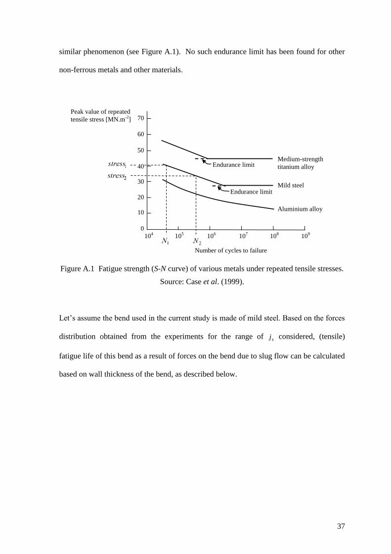
similar phenomenon (see Figure A.1). No such endurance limit has been found for other
non-ferrous metals and other materials.
Figure A.1 Fatigue strength (S-N curve) of various metals under repeated tensile stresses.
Source: Case et al. (1999).
Let’s assume the bend used in the current study is made of mild steel. Based on the forces
distribution obtained from the experiments for the range of sj considered, (tensile)
fatigue life of this bend as a result of forces on the bend due to slug flow can be calculated
based on wall thickness of the bend, as described below.
70
60
50
40
30
20
10
0
105
104
107
106
109
108
Medium-strength
titanium alloy
Mild steel
Aluminium alloy
Endurance limit
Endurance limit
Number of cycles to failure
Peak value of repeated
tensile stress [MN.m-2
]
38
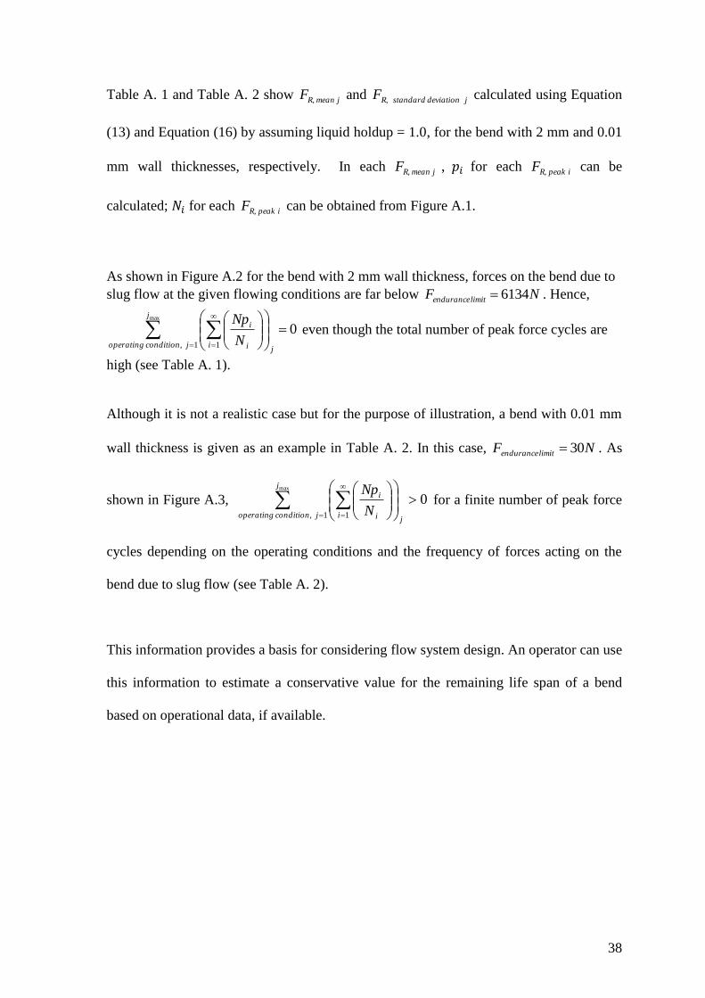
Table A. 1 and Table A. 2 show j meanR,F and j deviation standardR,F calculated using Equation
(13) and Equation (16) by assuming liquid holdup = 1.0, for the bend with 2 mm and 0.01
mm wall thicknesses, respectively. In each j meanR,F , 𝑝𝑖 for each i peakR,F can be
calculated; 𝑁𝑖 for each i peakR,F can be obtained from Figure A.1.
As shown in Figure A.2 for the bend with 2 mm wall thickness, forces on the bend due to
slug flow at the given flowing conditions are far below NF limit endurance 6134 . Hence,
0max
1 1
j
jcondition, operatingj
i i
i
N
Np even though the total number of peak force cycles are
high (see Table A. 1).
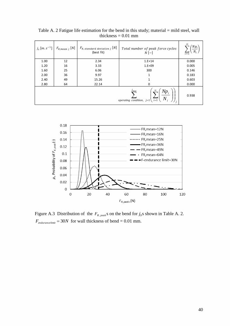
Although it is not a realistic case but for the purpose of illustration, a bend with 0.01 mm
wall thickness is given as an example in Table A. 2. In this case, NF limit endurance 30 . As
shown in Figure A.3, 0max
1 1
j
jcondition, operatingj
i i
i
N
Np for a finite number of peak force
cycles depending on the operating conditions and the frequency of forces acting on the
bend due to slug flow (see Table A. 2).
This information provides a basis for considering flow system design. An operator can use
this information to estimate a conservative value for the remaining life span of a bend
based on operational data, if available.
39
Table A. 1 Fatigue life estimation for the bend in this study; material = mild steel, wall
thickness = 2 mm
Figure A.2 Distribution of the peak,RF s on the bend for 𝑗𝑠s shown in Table A. 1.
NF limit endurance 6134 for wall thickness of bend = 2 mm.
1.00 12 2.34 1.E+250 0.000
1.20 16 3.33 1.E+250 0.000
1.60 25 6.06 1.E+250 0.000
2.00 36 9.97 1.E+250 0.000
2.40 49 15.26 1.E+250 0.000
2.80 64 22.14 1.E+250 0.000
0.000
max
1 1
j
jcondition, operatingj
i i
i
N
Np
𝑁𝑝𝑖𝑁𝑖
𝑖
𝑗𝑠 𝑁 𝑠 𝑖 𝑖 𝑁
(best fit) 𝑝
𝑁
40
Table A. 2 Fatigue life estimation for the bend in this study; material = mild steel, wall
thickness = 0.01 mm
Figure A.3 Distribution of the peak,RF s on the bend for 𝑗𝑠s shown in Table A. 2.
NF limit endurance 30 for wall thickness of bend = 0.01 mm.
1.00 12 2.34 1.E+14 0.000
1.20 16 3.33 1.E+09 0.005
1.60 25 6.06 300 0.146
2.00 36 9.97 1 0.183
2.40 49 15.26 1 0.603
2.80 64 22.14 0 0.000
0.938
𝑁𝑝𝑖𝑁𝑖
𝑖
max
1 1
j
jcondition, operatingj
i i
i
N
Np
𝑗𝑠 𝑁 𝑠 𝑖 𝑖 𝑁
(best fit) 𝑝
𝑁
41
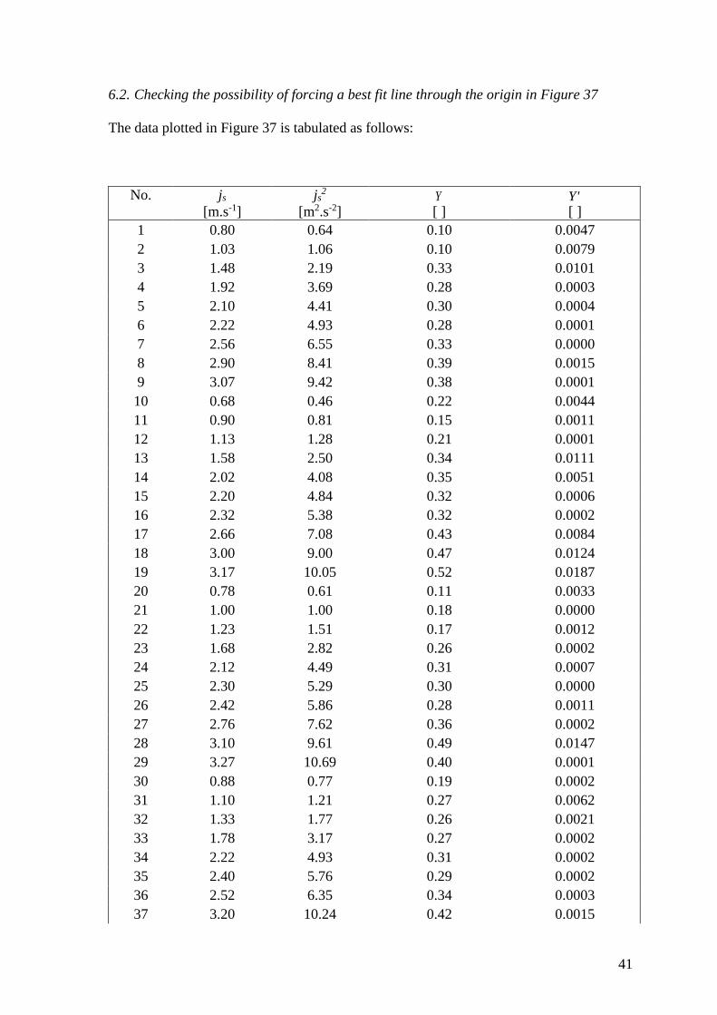
6.2. Checking the possibility of forcing a best fit line through the origin in Figure 37
The data plotted in Figure 37 is tabulated as follows:
No. js js2 Y 'Y
[m.s-1] [m2.s-2] [ ] [ ]
1 0.80 0.64 0.10 0.0047
2 1.03 1.06 0.10 0.0079
3 1.48 2.19 0.33 0.0101
4 1.92 3.69 0.28 0.0003
5 2.10 4.41 0.30 0.0004
6 2.22 4.93 0.28 0.0001
7 2.56 6.55 0.33 0.0000
8 2.90 8.41 0.39 0.0015
9 3.07 9.42 0.38 0.0001
10 0.68 0.46 0.22 0.0044
11 0.90 0.81 0.15 0.0011
12 1.13 1.28 0.21 0.0001
13 1.58 2.50 0.34 0.0111
14 2.02 4.08 0.35 0.0051
15 2.20 4.84 0.32 0.0006
16 2.32 5.38 0.32 0.0002
17 2.66 7.08 0.43 0.0084
18 3.00 9.00 0.47 0.0124
19 3.17 10.05 0.52 0.0187
20 0.78 0.61 0.11 0.0033
21 1.00 1.00 0.18 0.0000
22 1.23 1.51 0.17 0.0012
23 1.68 2.82 0.26 0.0002
24 2.12 4.49 0.31 0.0007
25 2.30 5.29 0.30 0.0000
26 2.42 5.86 0.28 0.0011
27 2.76 7.62 0.36 0.0002
28 3.10 9.61 0.49 0.0147
29 3.27 10.69 0.40 0.0001
30 0.88 0.77 0.19 0.0002
31 1.10 1.21 0.27 0.0062
32 1.33 1.77 0.26 0.0021
33 1.78 3.17 0.27 0.0002
34 2.22 4.93 0.31 0.0002
35 2.40 5.76 0.29 0.0002
36 2.52 6.35 0.34 0.0003
37 3.20 10.24 0.42 0.0015
42
38 3.37 11.36 0.39 0.0000
39 0.98 0.96 0.19 0.0000
40 1.20 1.44 0.20 0.0000
41 1.43 2.04 0.19 0.0011
42 1.88 3.53 0.19 0.0056
43 2.32 5.38 0.23 0.0048
44 2.50 6.25 0.27 0.0027
45 2.62 6.86 0.27 0.0031
46 2.96 8.76 0.31 0.0024
47 3.30 10.89 0.34 0.0028
48 3.47 12.04 0.35 0.0035
49 1.98 3.92 0.20 0.0053
50 2.42 5.86 0.21 0.0112
51 2.60 6.76 0.22 0.0111
52 2.72 7.40 0.28 0.0035
53 3.06 9.36 0.32 0.0028
54 3.40 11.56 0.34 0.0031
55 3.57 12.74 0.36 0.0031
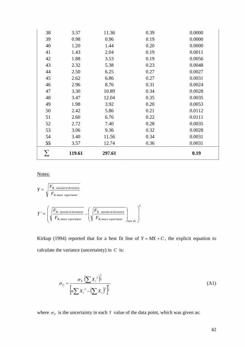
119.61 297.61 0.19
Notes:
Y = experiment meanR,
deviation standardR,
F
F
Y’ =
2
fit bestexperiment meanR,
deviation standardR,
experiment meanR,
deviation standardR,
F
F
F
F
Kirkup (1994) reported that for a best fit line of CMXY , the explicit equation to
calculate the variance (uncertainty) in C is:
21
22
2
12
ii
iY
C
XXn
X (A1)
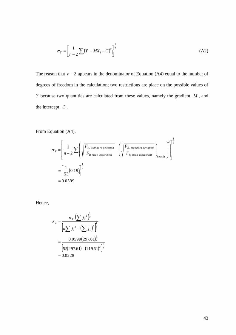
where Y is the uncertainty in each Y value of the data point, which was given as:
43
2
1
2
2
1
CMXY
niiY (A2)
The reason that 2n appears in the denominator of Equation (A4) equal to the number of
degrees of freedom in the calculation; two restrictions are place on the possible values of
Y because two quantities are calculated from these values, namely the gradient, M , and
the intercept, C .
From Equation (A4),
05990
19053
1
2
1
2
1
2
1
2
.
.
F
F
F
F
nfit best
experiment meanR,
deviation standardR,
experiment meanR,
deviation standardR,
Y
Hence,
02280
611196129755
6129705990
2
12
2
1
2
122
2
12
.
..
..
jjn
j
ss
sY
C

44
Notation
A Area [ 2m ]
C Constant [ ]
D Pipe diameter [ m ]
F Force [ N ]
g Gravitational acceleration [ -2m.s ]
h Liquid height (above pipe base) [m]
H
Hold-up, AAH kk
where k is the corresponding fluid phase.
[ ]
LH Liquid hold-up in the liquid slug body, AAH LL [ ]
ID Internal diameter [mm]
j Superficial velocity (i.e. AQ ) [ -1m.s ]
sj Superficial slug velocity, GLs jjj [ -1m.s ]
l Length [ m ]
el Elongation [m]
M Slope of a linear correlation [ ]
N Number of slugs or force cycles [ ]
iN Expected number of cycles to failure at istress or iF [ ]
n Number of samples [ ]
in Cycles at istress or iF [ ]
P Absolute pressure [ Pa ]
p Probability [ ]
R Bend radius (centre line) [ m ]
t Time [ s ]
45
u Actual velocity [ -1m.s ]
su Slug velocity, 41.02.1 ss ju [ -1m.s ]
X Independent variable in a linear correlation CMXY [ ]
x x direction [ ]
Y Dependent variable in a linear correlation CMXY [ ]
y y direction [ ]
Greek Symbols
Angle as shown in Figure 5 [rad]
Angle of bend [rad]
Dynamic viscosity [ Pa.s ]
Angular velocity [ -1rad.s ]
1423. [ ]
Density [ -3kg.m ]
Surface tension [ -1N.m ]
C Standard error of constant C in CMXY [ ]
M Standard error of slope M in CMXY [ ]
Y Standard error of variable Y in CMXY [ ]
Angular coordinate in polar coordinates (see Figure 4) [ rad ]
Subscripts
A See Figure 4: when liquid enters the section, A = liquid and B = gas: when
gas enters the section, A = gas and B = liquid.

46
'a Point 'a in Figure 4
B See Figure 4: when liquid enters the section, A = liquid and B = gas: when
gas enters the section, A = gas and B = liquid.
'b Point 'b in Figure 4
'c Point 'c in Figure 4
d Downstream pipe after the bend
'd Point 'd in Figure 4
'e Point 'e in Figure 4
G Gas phase
i Inside pipe (in Equation (2) and Equation (3))
i Integer number i -th (other than in Equation (2) and Equation (3))
j Integer number j -th
sj Superficial velocity
L Liquid phase
l Length
M Slope of a linear correlation, CMXY
max Maximum
mean Mean of the peak forces identified from statistical analysis
o Outside pipe
peak The largest force during transit of a slug unit
PFM Piston Flow Model
R Resultant
47
s Slug unit
su Slug velocity
x x - direction
y y - direction
Acknowledgements
This work has been undertaken within the second stage of the Transient Multiphase Flows
Co-ordinated research project. The authors wish to acknowledge the contributions made
to this project by the Engineering and Physical Sciences Research Council (EPSRC) and
to the following industrial organisations:- ABB; AEA Technology; BG International; BP
Amoco Exploration; Chevron; Conoco; Granherne; Institutt for Energiteknikk; Institut
Francais du Petrole; Marathon Oil; Mobil North Sea; Norsk Hydro; Scandpower;
TotalElfFina. The authors wish to express sincere gratitude for this support. Dr. Tay was
funded by Cambridge Commonwealth Trust Bursary and Churchill College Jafar
Research Studentship; these financial assistances are also gratefully acknowledged.
References
Alexander J. M. & Brewer R. C. (1963). Manufacturing properties of materials, Van
Nostrand Reinhold Company.
Case J., Chilver L. & Ross C. T. F. (1999). Strength of materials and structures, 4th
edition, Arnold.

48
Cook G. & Claydon P.W. (1992). Design life prediction of flexible riser systems,
MARINFLEX 92 Conference on Flexible Pipes, Umbilicals, Marine Cables.
Fairhurst, C. P. (1983). Two-phase transient phenomena in oil production flowlines,
BHRA The Fluid Engineering Centre.
Gatts R. R. (1961). Application of a cumulative damage concept to fatigue, Journal of
Basic Engineering, 529-540.
Goodfellow Associates. (1986). Offshore engineering: Development of small oilfields,
Graham and Trotman Limited.
Gregory, G. A., Nicholson, M. K., & Aziz K. (1978). Correlation of the liquid volume
fraction in the slug for horizontal gas-liquid slug flow. International Journal of
Multiphase Flow, 4, 33-39.
Gurney T. R. (1968). Fatigue of welded structures, Cambridge University Press.
Hargreaves, C. R., & Slocombe, R. W. (1998). Measurement of the forces on bends in
(oil) pipelines due to multiphase flow. Part II Report, 1998/53, University of
Cambridge, Department of Chemical Engineering.
Hilsenkopf P. (1988). Experimental study of behaviour and functional capability of
ferritic steel elbows and austenitic stainless steel thin-walled elbows, International
Journal of Pressure Vessels & Piping, 33, 111-128.
Kirkup L. (1994). Experimental methods: An introduction to the analysis and presentation
of data, John Wiley & Sons.

49
Kitching R. (1979). Limit moment for a smooth pipe bend under in-plane bending,
International Journal of Mechanical Science, 21, 731-738.
Klesnil M. & Lukáš P. (1992). Fatigue of metallic materials, 2nd revised edition, Elsevier.
Malnes D. (1987). Slug flow in vertical, horizontal and inclined pipes, Report IFE/KR/E-
83/002 V. Institute for Energy Technology, Norway.
Miner M.A. (1945). Cumulative damage in fatigue, Journal of Applied Mechanics, 12,
1945.
Pope J. A. (1959). Metal Fatigue, Chapman & Hall.
Santana B. W., Fezner D., Edwards N. W. & Haupt R. W. (1993) Program for improving
multiphase slug force resistance at Kuparuk river unit processing facilities, SPE
26104, Richardson, Texas.
Shalaby M. A. & Younan M. Y. A. (1999). Limit loads for pipe elbows subjected to in-
plane opening moments and internal pressure, Journal of Pressure Vessel
Technology, 121, 17-23.
Shalaby M. A. & Younan M. Y. A. (1998). Limit loads for pipe elbows with internal
pressure under in-plane closing moments, Journal of Pressure Vessel Technology-
Transactions, 120, 35-42.
Tay B.L. & Thorpe R.B. (2014). Hydrodynamic forces acting on a pipe bends in gas-
liquid slug flow. Chemical Engineering Research and Design, 92, 812-825.

50
Tay B.L. & Thorpe R.B. (2004). Effects of liquid physical properties on the forces acting
on a pipe bend in gas-liquid slug flow. Chemical Engineering Research and
Design, 82, 344 - 356.
Tay, B. L., & Thorpe, R. B. (2002). Forces on pipe bends due to slug flow. The
proceeding of 3rd North American Multiphase Technology Conference, Banff, 281-
300.
Tottle C. R. (1984). An encyclopedia of metallurgy and materials, Macdonald and Evans.