Radu Grosu Vienna University of Technology

Hybrid Systems Modeling, Analysis and Control

Lecture 11 Constraint Satisfaction

Using Interval Approximation

Linear Classifiers with Hard Threshold x 2

: sur

face

-wav

e m

agni

tude

x1: body-wave magnitude

−Linear: A hyperplane. E.g. − 4.9 + 1.7x1 − x2 = 0

−Explosions: − 4.9 + 1.7x1 − x2 > 0

−Earthquake: − 4.9 + 1.7x1 − x2 < 0 Decidable!

! eartquake • nuclear explosion

Decision boundary: Surface that separates two classes

Polynomial Constraints

Theorem (Tarski 1949): The first-order theory of real-closed ordered fields is decidable.

Proof: FOT (R, ≤ ,+,×) admits quantifier elimination.

x2 + y2 − 1 = 0 ∧ y − x2 = 0

x

y

Polynomial Constraints

Theorem (Tarski 1949): The first-order theory of real-closed ordered fields is decidable.

Complexity: ExpExp in # alternations, Exp in # vars

x2 + y2 − 1 = 0 ∧ y − x2 = 0

x

y

What About Certificates?

Certificate: Satisfying valuation (solution) Quantifier-free case: Eg. x2 = 2

Question: How to represent the solution?

−Linear case: Rational numbers. Eg. 3x = 2 ⇒ x = 2 / 3

−Polynomial case: Real algebraic numbers (unintuitive)

−Non-polynomial case f(x) = 0: An approx algorithm

Given: desired precision k ∈NReturns r ∈Q: ∃x. |x − r| ≤ 10−k ∧ f(x) = 0

What About Certificates?

Certificate: Satisfying valuation (solution) Quantifier-free case: Eg. x2 = 2

Question: How to represent the solution?

−Linear case: Rational numbers. Eg. 3x = 2 ⇒ x = 2 / 3

−Polynomial case: Real algebraic numbers (unintuitive)

−Non-polynomial case f(x) = 0: An approx algorithm

Given: desired precision k ∈NReturns r ∈Q: |f(r)| ≤ 10−k

Non-Polynomial Constraints (NPC)

What about: FOT (R, ≤ ,+,×,sin) ?

−Undecidable: A Would allow encoding of polynomial diophantine equations (PDE)

f(x,y) > 0

f(x,y) < 0

x

y

−PDE: Known to be undecidable (Matiyasevich, 1970)

Fixing Precision of NPC

x

y

f(x,y) < 0

f(x,y) > 0

What about: FOT (R, ≤ ,+,×,sin) ?

Exponential: In the number of boxes!

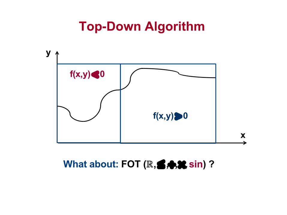
Top-Down Algorithm

x

y

f(x,y) < 0

f(x,y) > 0

What about: FOT (R, ≤ ,+,×,sin) ?

Top-Down Algorithm

x

y

f(x,y) < 0

f(x,y) > 0

What about: FOT (R, ≤ ,+,×,sin) ?

Top-Down Algorithm

x

y

f(x,y) < 0

f(x,y) > 0

What about: FOT (R, ≤ ,+,×,sin) ?

Top-Down Algorithm

x

y

f(x,y) < 0

f(x,y) > 0

What about: FOT (R, ≤ ,+,×,sin) ?

Top-Down Algorithm

x

y

f(x,y) < 0

f(x,y) > 0

What about: FOT (R, ≤ ,+,×,sin) ?

Top-Down Algorithm

x

y

f(x,y) < 0

f(x,y) > 0

What about: FOT (R, ≤ ,+,×,sin) ?

Infinite precision: May not terminate!

Robust Constraints

Real CPS (biology/engineered): Satisfy robust properties

−Satisfiability: Does not change under perturbations

c2

! eartquake • nuclear explosion

c1

x1: body-wave magnitude

x 2: s

urfa

ce-w

ave

mag

nitu

de

Robust Constraints

Constraint ϕ is robust iff

Real CPS (biology/engineered): Satisfy robust properties

−Satisfiability: Does not change under perturbations

x2 ≤ 0 ⇒ x2 ≤ −0.00001 −Not robust:

x2 ≤ 1 ⇒ x2 ≤ +0.99999 −Robust:

−Constraint distance: d(ϕ,ϕ') ! (ϕ ≡upto cst c

ϕ') ? c : ∞

−There is an ε such that

−For all ϕ ' with d(ϕ,ϕ') ≤ ε

ϕ and ϕ ' are equi-satifiable

Quasi Deciadable Problems

A problem is quasi decidable iff:

−There is an algorithm that

−Correctly checks satifiability and −Terminates on all robust instances

Theorem (Ratschan 2002):

−FOT (R, ≤ +, ×, exp, sin, ...) is quasi decidable

Assumptions:

−All variables are bounded (in some interval)

−Shortcut: f = 0 ≡ (f ≤ 0 ∧ f ≥ 0)

Implementation: http://rsolver.sourceforge.net

Not Quasi Deciadable Problems

Theorem (Clarke/Gao 2011):

−δ-Satisfiability is decidable

x

y

f(x,y) < 0

f(x,y) > 0

δ do not know

Algorithm: Quantifier-Free Conjunctive

Box (hyper-rectangle): Cartesian product of intervals

−Given ϕ: Conjunction of ≤ using +, ×, exp, sin

Uses algorithms for both sat and unsat: Why?

−Due to undecidability failure to prove sat

−Box B: Providing an interval for each variable

Quasi-Satisfiability Algorithm

−Decide: Sat or Unsat

−Does not imply unsat and vice versa −Later on can use information from each other

Search for Sat

Satisfiability: Statement over one valuation −Good search method: Suffices

−Local search examples: Newton-type methods

−Iteratively refine the grid

−Local search: Start from this points

x

y

f(x,y) < 0

f(x,y) > 0

−Approximation errors: Floating-point rounding OK

Search for Unsat: Branch and Bound

Non-Satisfiability: Statement over an uncountable set

−Symbolic representation: Necessary

S = test(ϕ,B) if (S = unsat) return S else

−Use: test(ϕ,B) ∈{unsat, unknown}

let B = B1 ∪B2 non-overlapping

Algorithm BB(ϕ,B): Either returns unsat or runs forever

if (BB(ϕ,B1) = BB(ϕ,B2) = unsat) return unsat

Can be interleaved: With satisfiability test

Test for Unsat

Works recursively: On the structure of ϕ −Special case: One single equality

−Input: f(x1,...,xn) = 0, B = intervals (I1,...,In)

{f(x1,...,xn) | x1 ∈I1,...,xn ∈In} ⊆ [f] (I1,...,In)

if (0 ∉[f](I1,...,In)) return unsat else unknown

Compute: [f] (I1,...,In), an inclusion of f, s.t:

Example:

x × y + 1 = 0

x ∈[2,3], y ∈[4,7] B = ([2,3],[4,7])

[2,3] [4,7]

x y

[8,21]

[×] [1,1]

[9,22]

[+]

1

Interval Arithmetic: Addition

Function [+] on intervals [a,a] and [b,b] is an inclusion:

[a,a] [+] [b,b] =

∅ if [a,a] = ∅ ∨ [b,b] = ∅[a + b,a + b] otherwise

⎧⎨⎪

⎩⎪

Example:

[8,21] [+] [1,1] = [9,22] [8,21] [1,1]

[9,22]

[+]

Proof: + does not have any local minimum Corners suffice

Interval Arithmetic: Multiplication

Function [×] on intervals [a,a] and [b,b] is an inclusion:

[a,a] [×] [b,b] =

∅ if [a,a] = ∅ ∨ [b,b] = ∅ [min{ab,ab,ab,ab}, max{ab,ab,ab,ab}] else

⎧⎨⎪

⎩⎪

Example:

[2,3] [×] [4,7] = [8,21] [2,3] [4,7]

[8,21]

[×]

Proof: × does not have any local minimum Corners suffice

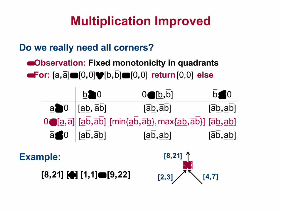
Multiplication Improved

Do we really need all corners?

b ≥ 0 0 ∈[b,b] b ≤ 0a ≥ 0 [ab, ab] [ab,ab] [ab,ab]

0 ∈[a,a] [ab,ab] [min{ab,ab}, max{ab,ab}] [ab,ab]a ≤ 0 [ab,ab] [ab,ab] [ab,ab]

Example:

[8,21] [+] [1,1] = [9,22] [2,3] [4,7]

[8,21]

[×]

−Observation: Fixed monotonicity in quadrants

−For: [a,a] = [0,0]∨ [b,b] = [0,0] return [0,0] else

Other Operations

What about exp, sin, cos?

−Observation: Exploit monotonicity!

Interval arithmetic: Given term t in vars x1 ∈I1,...,xn ∈In

[t](I1,...,In) =

Ii if t = xi

[c,c] if t = c

[s]([t1](I1,...,In),...,[tk ](I1,...,In)) if t = s(t1,..., tk )s ∈{+,×,exp,...}

⎧

⎨⎪⎪

⎩⎪⎪

Fundamental theorem of interval arithmetic:

−For a term e, its interval extension [e] is an inclusion.

Properties of Inclusions

Width of a box: w([a1,b1] × ... × [an,bn]) = max

i∈{1,...,n}| bi − ai |

−Thin: iff w(B) = 0 ⇒ w([f](B)) = 0 An inclusion [f] of a function f is:

where: f(B) ! {f(x) | x ∈B}, [A] ! [inf A, sup A]

−Convergent: iff ∀B1 ⊇ ... ⊇Bn.limn→∞ w(Bn) = 0 ⇒ w([f](Bn)) = 0

−Monotonic: iff B1 ⊆ B2 ⇒ [f](B1) ⊆ [f](B2)

−Optimal: iff [f](B) = [f(B)]

Theorem:

If f: Rn → R does not contain any variable more than once then [f] is optimal.

Dependency Problem

Interval arithmetic forgets equality between variables:

[x − x]([-1,1]) = [x]([-1,1]) [−] [x]([-1,1])

Diff ways of writing the same exp, diff results:

[a × (b + c)](B) ⊆ [a × b + a × c)](B)

There are systematic methods for dealing with the dependency problem: [Neumaier 1990, Moore 2009]

[x × y + x]([1,2],[-1,-1]) = ([x]([1,2]) [×] [y]([-1,-1])) [+] [x]([1,2])

= [-1,1] [−] [-1,1] = [-2,2] ⊃ [0,0]

= ([1,2] [×] [-1,-1]) [+] [1,2]

= [-2,-1] [+] [1,2] = [-1,1] ⊃ [0,0]

Wrapping Effect

Rotation matrix:

At =cos(t) sin(t)−sin(t) cos(t)

⎛

⎝⎜

⎞

⎠⎟

Appears in several contexts especially ODE solving

Exponential blow-up

−Smaller t makes things worse

−In the limit box eplodes by a

−A factor of e2π ≈ 535 per revolution

Partial solution: Coordinate transfomations

Efficiency of Branch-And-Bound

Curse of dimensionality:

−Halving boxes in n-dim: 2n boxes

−Branching does not scale in problem dim

−Can one deduce more without branching?

Example

x − 99 = 0 ∧ y − 99 = 0, x ∈[0,100], y ∈[0,100]

x

y

100

100

Example

x − 99 = 0 ∧ y − 99 = 0, x ∈[0,100], y ∈[0,100]

x

y

100

100

Example

x − 99 = 0 ∧ y − 99 = 0, x ∈[0,100], y ∈[0,100]

x

y

100

100

Example

x − 99 = 0 ∧ y − 99 = 0, x ∈[0,100], y ∈[0,100]

x

y

100

100

Example

x − 99 = 0 ∧ y − 99 = 0, x ∈[0,100], y ∈[0,100]

x

y

100

100

Example

x − 99 = 0 ∧ y − 99 = 0, x ∈[0,100], y ∈[0,100]

x

y

100

100

Example

x − 99 = 0 ∧ y − 99 = 0, x ∈[0,100], y ∈[0,100]

x

y

100

100

Example

x − 99 = 0 ∧ y − 99 = 0, x ∈[0,100], y ∈[0,100]

x

y

100

100

Example

x − 99 = 0 ∧ y − 99 = 0, x ∈[0,100], y ∈[0,100]

x

y

100

100

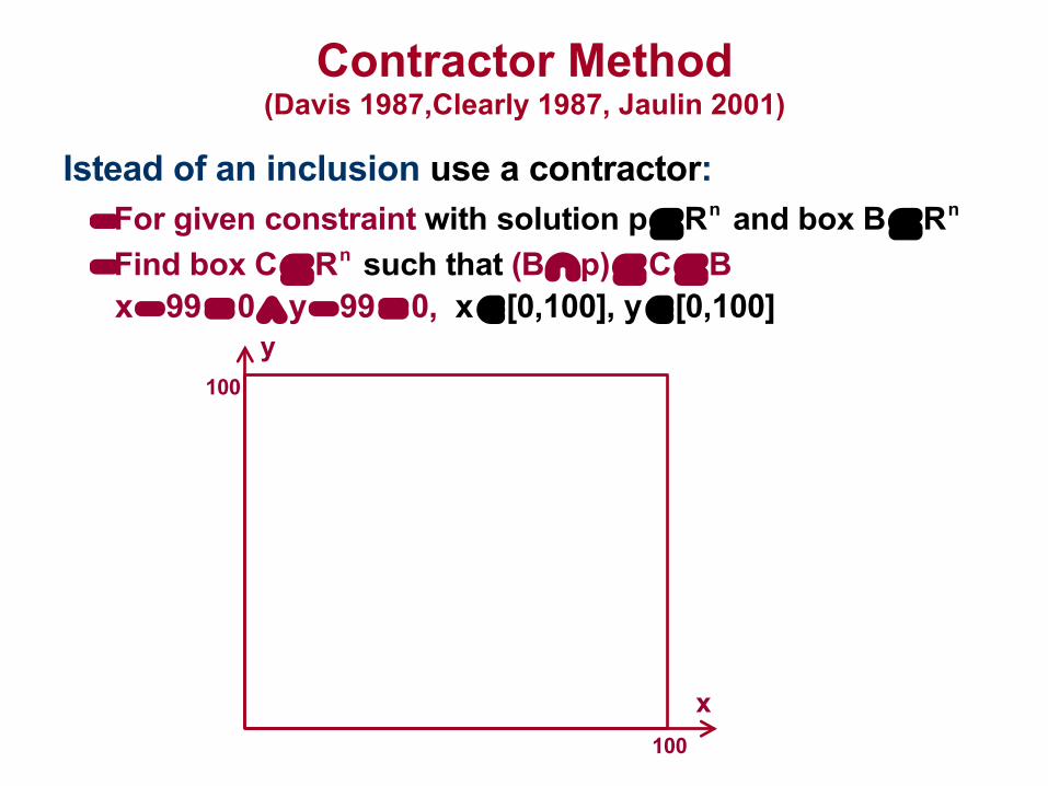
Contractor Method (Davis 1987,Clearly 1987, Jaulin 2001)

Istead of an inclusion use a contractor:

−For given constraint with solution p ⊆ Rn and box B ⊆ Rn

−Find box C ⊆ Rn such that (B∩p) ⊆ C ⊆ B

x − 99 = 0 ∧ y − 99 = 0, x ∈[0,100], y ∈[0,100]

x

y

100

100

Contractor Method (Davis 1987,Clearly 1987, Jaulin 2001)

x

y

100

100

Istead of an inclusion use a contractor:

−For given constraint with solution p ⊆ Rn and box B ⊆ Rn

−Find box C ⊆ Rn such that (B∩p) ⊆ C ⊆ B

x − 99 = 0 ∧ y − 99 = 0, x ∈[0,100], y ∈[0,100]

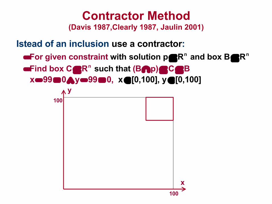
Contractor Method (Davis 1987,Clearly 1987, Jaulin 2001)

Istead of an inclusion use a contractor:

−For given constraint with solution p ⊆ Rn and box B ⊆ Rn

−Find box C ⊆ Rn such that (B∩p) ⊆ C ⊆ B

x − 99 = 0 ∧ y − 99 = 0, x ∈[0,100], y ∈[0,100]

A contractor ⌢p of a constraint p is called optimal iff:

−For every box B: ⌢p(B) = (B∩p)

−In practice: Optimal up to rounding

Computing Contractors: Sum

sum ! {(x,y,z) | x + y = z}

Contractor:

Need hull of projection to 3 axes within B = Ix × Iy × Iz

i π1(sum∩ Ix × Iy × Iz ) = Ix ∩ (Iz − Iy )

i π2(sum∩ Ix × Iy × Iz ) = Iy ∩ (Iz − Ix )

i π3(sum∩ Ix × Iy × Iz ) = Iz ∩ (Ix + Iy )

i s⌢um(Ix × Iy × Iz ) = Ix ∩ (Iz − Iy ) × Iy ∩ (Iz − Ix ) × Iz ∩ (Ix + Iy )

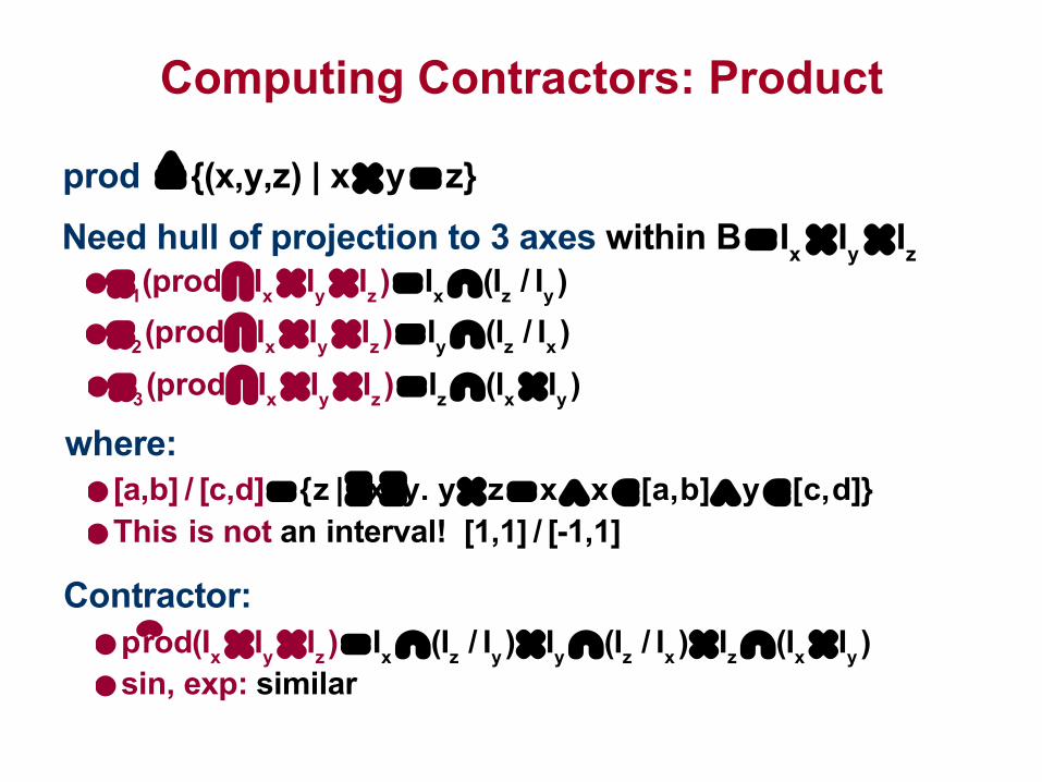
Computing Contractors: Product

prod ! {(x,y,z) | x × y = z}

where:

Need hull of projection to 3 axes within B = Ix × Iy × Iz

i π1(prod∩ Ix × Iy × Iz ) = Ix ∩ (Iz / Iy )

i π2(prod∩ Ix × Iy × Iz ) = Iy ∩ (Iz / Ix )

i π3(prod∩ Ix × Iy × Iz ) = Iz ∩ (Ix × Iy )

i [a,b] / [c,d] = {z | ∃x∃y. y × z = x ∧ x ∈[a,b]∧ y ∈[c,d]}

Contractor:

i p⌢rod(Ix × Iy × Iz ) = Ix ∩ (Iz / Iy ) × Iy ∩ (Iz / Ix ) × Iz ∩ (Ix × Iy )

i This is not an interval! [1,1] / [-1,1]

i sin, exp: similar

Contractors: Conjunction c1∧...∧cn

C = {c1,...,cn}

while (∃c ∈C. ⌢c(B) ≠ B) B =

⌢c(B)

Contractors: Conjunction c1∧...∧cn

C = {c1,...,cn}

while (∃c ∈C. ⌢c(B) ≠ B) B =

⌢c(B)

Contractors: Conjunction c1∧...∧cn

C = {c1,...,cn}

while (∃c ∈C. ⌢c(B) ≠ B) B =

⌢c(B)

Contractors: Conjunction c1∧...∧cn

C = {c1,...,cn}

while (∃c ∈C. ⌢c(B) ≠ B) B =

⌢c(B)

Termination? Optimal?

Contractors: Conjunction c1∧...∧cn

C = {c1,...,cn}

while (∃c ∈C. ⌢c(B) ≠ B) B =

⌢c(B)

Termination? Optimal? x − y = 0 ∧ x + y = 0

Contractors: Constraints with General Terms

Optimal?

Example: x × y + sin(z) = 0

i x × y = v1 ∧ sin(z) = v2 ∧ v1 + v2 = v3 ∧ v3 = 0

i Primitive constraints: x + y = z, x × y = z, sin(x) = x,...

i No,but at least as good as interval arithmetic

i RSolver implementation, dReal implementation