HYBRID SOFT SOIL TIRE MODEL (HSSTM). PART I: TIRE …world situation. In this regard, an...

UNCLASSIFIED: Distribution Statement A. Approved for public release.

__________________________________________________________________________________________________ Disclaimer: Reference herein to any specific commercial company, product, process, or service by trade name, trademark, manufacturer, or otherwise, does not necessarily constitute or imply endorsement, recommendation, or favoring by the United States Government or the Department of the Army (DoA). The opinions of the author expressed herein do not necessarily state or reflect those of the United States Government or the DoA, and shall not be used for advertising or product endorsement purposes. __________________________________________________________________________________________________

HYBRID SOFT SOIL TIRE MODEL (HSSTM).

PART I: TIRE MATERIAL AND STRUCTURE MODELING

Taheri, Sh.a,1, Sandu, C.a , Taheri, S.a, Gorsich, D.b

aDepartment of Mechanical Engineering, Virginia Tech, Blacksburg, VA, USA

bU.S. Army TARDEC, MI, USA

Abstract

In order to model the dynamic behavior of the tire on soft soil, a lumped mass discretized tire model using

Kelvin-Voigt elements is developed. To optimize the computational time of the code, different techniques

were used in memory allocation, parameter initialization, code sequence, and multi-processing. This has

resulted in significant improvements in efficiency of the code that can now run close to real time and therefore

it is suitable for use by commercially available vehicle simulation packages.

Model parameters are obtained using a validated finite element tire model, modal analysis, and other

experimental test procedures. Experimental tests were performed on the Terramechanics rig at Virginia Tech.

The tests were performed on different terrains (such as sandy loam) and tire force and moments, soil sinkage,

and tire deformation data were collected for various case studies based on a design of experiment matrix. This

data, in addition to modal analysis data were used to validate the tire model. Furthermore, to study the validity

of the tire model, simulations at conditions similar to the test conditions were performed on a quarter car

model. The results have indicated the superiority of this model as compared to other lumped parameter models

currently available.

Keywords: Wheeled Vehicle, Terramechanics, Off-Road, Deformable Terrain, Tire Model, Soil, Parameterization, Mobility

1Corresponding author email address:

[email protected]

Report Documentation Page Form ApprovedOMB No. 0704-0188

Public reporting burden for the collection of information is estimated to average 1 hour per response, including the time for reviewing instructions, searching existing data sources, gathering andmaintaining the data needed, and completing and reviewing the collection of information. Send comments regarding this burden estimate or any other aspect of this collection of information,including suggestions for reducing this burden, to Washington Headquarters Services, Directorate for Information Operations and Reports, 1215 Jefferson Davis Highway, Suite 1204, ArlingtonVA 22202-4302. Respondents should be aware that notwithstanding any other provision of law, no person shall be subject to a penalty for failing to comply with a collection of information if itdoes not display a currently valid OMB control number.

1. REPORT DATE 28 APR 2015 2. REPORT TYPE

3. DATES COVERED 00-00-2015 to 00-00-2015

4. TITLE AND SUBTITLE Hybrid Soft Soil Tire Model (HSSTM) Part I: Tire Material andStructure Modeling

5a. CONTRACT NUMBER

5b. GRANT NUMBER

5c. PROGRAM ELEMENT NUMBER

6. AUTHOR(S) 5d. PROJECT NUMBER

5e. TASK NUMBER

5f. WORK UNIT NUMBER

7. PERFORMING ORGANIZATION NAME(S) AND ADDRESS(ES) US Army RDECOM-TARDEC,6501 E. 11 Mile Road,Warren,MI,48397-5000

8. PERFORMING ORGANIZATIONREPORT NUMBER

9. SPONSORING/MONITORING AGENCY NAME(S) AND ADDRESS(ES) 10. SPONSOR/MONITOR’S ACRONYM(S)

11. SPONSOR/MONITOR’S REPORT NUMBER(S)

12. DISTRIBUTION/AVAILABILITY STATEMENT Approved for public release; distribution unlimited

13. SUPPLEMENTARY NOTES

14. ABSTRACT See Report

15. SUBJECT TERMS

16. SECURITY CLASSIFICATION OF: 17. LIMITATION OF ABSTRACT Same as

Report (SAR)

18. NUMBEROF PAGES

40

19a. NAME OFRESPONSIBLE PERSON

a. REPORT unclassified

b. ABSTRACT unclassified

c. THIS PAGE unclassified

Standard Form 298 (Rev. 8-98) Prescribed by ANSI Std Z39-18

Journal of Terramechanics Page 2 of 40

UNCLASSIFIED

1 Introduction

The tire forces and moments depend on the structural behavior of the tire, as well as tire-terrain interaction.

Therefore, based on the simulation application (e.g., handling, ride, mobility, durability), and type of the terrain (e.g.,

deformable, non-deformable, even, uneven) the approach for modeling the tire and the terrain would be different. The

tire models that are used for vehicle simulation on mainly non-deformable terrains, such as FTire [1], RMOD-K [2,

3], CDTire [4], can be categorized based on usage, accuracy, computational efficiency, and degree of parameterization.

The number of degrees-of-freedom (DOFs) and consequently the computational effort in these models can be sorted

from empirical models (lowest) to finite element models (highest).

A direct application of an on-road tire model to simulate tire performance on soft soil is not possible. This is due

to the fact that traveling on deformable terrain raises issues for which on-road tire models do not account for.

Moreover, the kinetics and kinematics of the tire on deformable terrains are subjected to different design and

operational factors, as well as field characteristics. These factors, in addition to the uncertainties that exist in their

parameterization, make the formulation of tire-terrain interaction a highly complex problem. Due to this complexity,

the number of tire models, similar to the one developed in this research that are usable in conjunction with multibody

dynamic vehicle simulation models, are limited.

The proposed process of developing the complete soft soil tire model can be divided into two main sub-processes

of mathematical modeling and physical modeling, as shown in Figure 1. For the mathematical modeling, different

components of the system, such as tire material, tire structure and tire-ground interaction are described using semi-

empirical mathematical correlations. Next, these mathematical models are implemented using a programing language,

such as MATLAB. The developed code is checked to confirm that the model is correctly implemented and is free of

errors. Meanwhile, a physical representation of the problem is essential to provide an insightful look into the real

world situation. In this regard, an experimental test rig is designed for conducting the related case studies. The type

and configuration of these experiments, which are required for validating and parameterizing the implemented sub-

models, are developed as a design of experiment table.


UNCLASSIFIED

Figure. 1 - Tire modeling on the soft soil: Modeling, simulation, and experimental procedures work flow.

Using the parameters derived for the computational model, simulations are performed at conditions similar to the

experiments. The results from this step are iteratively generated and compared to the test data until the acceptable

agreement is achieved. In case the correlation accuracy was not achieved after extensive simulation iterations, the

judgment is made whether to make changes to one of the sub-models, experimental setup, parameterization

procedures, or all of the above. In the following sections, first a brief literature survey for the available tire models

that are designed for estimating the tire performance on deformable surfaces is given. Next, steps that are required for

accurately characterizing the tire structure behavior are elaborated in more details. It should be mentioned that the

development of the tire-ground interaction model is discussed in a companion paper [5]. Representative simulation

results for the newly developed tire model, called Hybrid Soft Soil Tire Model (HSSTM) are discussed.

2 Literature Survey

As mentioned earlier, the main challenge in studying the behavior of the vehicle in off-road condition is

characterizing the tire-terrain interaction. Throughout the years, a wide variety of models have been developed for


UNCLASSIFIED

formulating and simulating this interaction. The degree of complexity for these models is based on the application,

accuracy, and computational cost. Generally, these models can be grouped into three main categories [6]: 1) Empirical

models, 2) semi-empirical models, and 3) physics-based models. The literature survey included in this paper is brief,

but the authors published an extensive review paper on this topic, and the reader is encouraged to refer to [6]

2.1 Empirical models

The empirical models use the experimental data of the tire response, and correlate it to the influential parameters

of the system via mathematical equations. One of the most famous empirical models is the Magic Formula Tire Model,

presented by Pacejka [7]. This model is based on the tire steady-state response data, and relates the tire forces and

moments to wheel pure slip values

Empirical models are very useful as simple tools for evaluating the performance of the vehicles in conditions

similar to the test environment and with tire properties similar to the test tire [2, 8-10]. Due to these limitations,

empirical models cannot be used for extrapolating the results to the problems outside the scope of the specific

experimental tests under which the data has been obtained. Thus, a new tire design concept or a new operating

condition for testing the tire performance cannot be studied using this family of tire models. The empirical models

developed for passenger and truck size tires do not scale perfectly to the smaller size tires, such as tires in robotic

applications and planetary exploration vehicles. Furthermore, empirical tire models require several sets of data for

their parameter estimation process that increases the cost of experimental procedure.

2.2 Physics based models

A tire on road is constantly excited by road unevenness with short and long wavelengths. Consequently, it operates

as a filter over the road roughness. Capturing the tire-road interaction for road inputs with high frequency (short

wavelengths), relative to the size of the contact patch, is more complex. The tire response at the spindle of the tire is

usually smoother than the shape of the obstacle. This behavior has two main reasons; first, when the tire travels over

an obstacle, such as a cleat, the forehead of the tire touches the obstacle before the wheel center. Therefore, the distance

traveled by the tire while interacting with an obstacle is longer than the length of the obstacle. Second, the tire has

some flexibility at its contact patch, which almost swallows the small irregularities during the enveloping process [11].

Capturing this filtering performance is the main motive for several physic-based tire models.


UNCLASSIFIED

Physics based models incorporate the physical principles and analytical methods to represent tire and terrain

structures in addition to their interaction [12]. This multi-disciplinary field of models incorporates applied

mathematics, numerical analysis, computational physics, and even computer graphics to evaluate the performance of

wheeled vehicles [13]. The degree of complexity varies from the simple models that consider tire as a rigid ring and

terrain as a spring-damper system to very detailed models that use finite element formulation for both tire and terrain

[14, 15].

2.3 Semi-empirical models

Mechanical behavior of the tire and tire-terrain depends on many aspects, such as tire geometrical and material

properties, in addition to terrain texture and frictional characteristics. Identifying all of these parameters and

correlating them to the vehicle performance using empirical closed-form formulations are limited to the similar test

conditions. On the other hand, using the simple physics-based methods to model the terrain can lead to significant

errors in both estimating model parameters and capturing terrain mechanics. This will ultimately cause the vehicle

response to deviate from the experimental data. One alternative numerical method for analyzing vehicle performance

is the semi-empirical models [16-19]. In this category of tire models, the tire structure is usually modeled by analytical

equations and the terrain is defined using empirically derived models [20]. These models are best nominees for

dynamic vehicle simulations because they are a trade-off between accuracy and computational efficiency [11-13].

The majority of the models in this field use the two-dimensional empirical formulation developed by Bekker and

Wong [21-28]. In these formulations, the tire is commonly considered as a rigid cylinder, and the normal and shear

stresses in the tire contact patch are expressed as functions of the tire kinetics and kinematic variables. Consequently,

the corresponding stress components are integrated over the contact patch to calculate the spindle forces, tire sinkage,

soil deformation, tire deflection, etc. The more sophisticated tire models use a finite element representation for either

tire structure or tire-ground interaction.

The proposed tire model is considered as a semi-empirical tire model because it takes a physics-based lumped

parameter approach for describing the tire structural response in addition to a semi-empirical method for characterizing

the tire-terrain interaction.


UNCLASSIFIED

3 Tire material modeling

A typical modern tire is manufactured from nearly 10-35 different components. Information about tire material

properties, processing, mixing, assembly, and curing are almost always confidential, and cannot be received from tire

companies. Furthermore, the material properties for the same tire from a manufacturer may vary, due to the

vulcanization process, for example. In order to accurately estimate the behavior of the tire components, elaborate

material models are needed. The parameterization of these models for individual materials in the tire requires

performing extensive experimental and analytical procedures, such as elastic and viscoelastic tests on individual tire

sections. This level of detail is required for calculating the accurate stress and strains in the tire structure, which would

be helpful in the design stage of the tire.

The main scope of this study is to estimate the tire mobility performance factors including forces and moments at

the tire spindle. Therefore, simplified methods are chosen for describing the tire material behavior, such as

hyperelasticity and viscoelasticity.

3.1 Hyperelasticity

A great portion of the tire structure consists of vulcanized elastomers, such as rubber material. Rubber has a

nonlinear and incompressible behavior toward loading, which is independent of the strain rate. This behavior is known

as hyperelasticity, and the material which shows this behavior is called green elastic material or hyperelastic. A

hyperelastic material differs from an elastic material in four main aspects:

The tire has a high stiffness in the initial step of loading, and dramatically softens in the unloading phase.

This phenomenon is known as Mullin’s effect.

Instead of having a hysteresis loop in the stress-strain curves of the loading cycle, the hyperelastic materials

have a simple equilibrium curve.

The hyperelastic materials exhibit different behavior in tension and compression. This is in contrast with the

Hooke’s law, which considers the stress to be proportional to strain. As a matter of fact, hyperelastic materials

such as rubber, have a higher stress magnitude in compression when compared to the tension for an identical

strain magnitude.


UNCLASSIFIED

Finally, a hyperelastic material has different modes of deformation that should be studied with respect to the

given loading conditions. Each deformation mode requires corresponding constants in the material model

that must be characterized experimentally. The choice of model constants and required parameterization tests

should be done with care in order to avoid false analytical system response quantities that are not present in

the experiments.

The hyperelasticity feature of the rubber should be enhanced with the viscoelasticity in order to precisely describe the

rate-dependent loading/unloading force-deflection characteristics of the tire.

3.2 Viscoelasticity

Viscoelastic materials show a combined elastic and viscous rate-dependent behavior when experiencing

deformation [29]. In elastic materials, once the applied stress or strain is removed, the specimen quickly returns to its

initial condition. On the other hand, viscous materials exhibit a resistance toward the shear flow developed due to the

applied stress or strain. In other words, upon applying a constant strain, the material creeps. Similarly, by applying a

constant stress, the strain increases and then eventually decreases with time.

The internal damping, rolling resistance, and thermal characteristics of a tire are associated with the viscoelastic

property of the rubber. Therefore, in order to properly quantify the transient response of the tire, the viscoelastic

material property should be incorporated. For small strains, the linear viscoelasticity assumption may be chosen. In

this case, the relaxation rate of the material is proportional to the immediate stress, and the total viscoelastic behavior

can be expressed using the superposition principle.

3.3 Modeling procedure

There are different mechanical models that can describe the combined hyperelastic viscoelastic characteristics of

a material. Each of the mechanical models considers a certain form of stress or strain response for the material under

different loading conditions. The hyperelasticity of the tire is modeled by interpolating the tire load vs. deflection data

in compression/tension loading/unloading scenarios. Using this approach allows us to define different loading stiffness

for loading and unloading paths.

To include viscoelasticity, three main models considered which are Maxwell model, Kelvin-Voigt model, and

Standard Linear Solid model [30]. For the Maxwell model, the viscoelasticity is modeled using a damping element


UNCLASSIFIED

(Newtonian dashpot) connected to a Hookean spring (stiffness element) in a series configuration. Considering the fact

that the Maxwell model exhibits the unrestricted flow of material during loading, it isn’t desirable for the rubber

element modeling. For the Kelvin-Voigt element, the stiffness and the damping elements are connected to each other

in a parallel configuration. The force-deflection characteristics of this model for force step input and deflection step

input are shown in Figure 2.

Figure. 2 - The force-deflection characteristics of the Kevin-Voigt model for force step input and deflection

step input.

For this type of element, the force-deflection relation under axial loading has the following form:

dt

dk

(1)

Where k is the axial stiffness, is the damping stiffness, is the element strain, and is the applied stress. It should

be noted that stress and strain of the element are analogous to the force and deflection. In the multi-axial loading the

equation of motion is written as

dt

deKeS

ij

ijij (2)

In which K is the time-dependent bulk modulus, and ijS is the element compliance. Another material model of interest

is the Standard Linear Model (SLM), which is a Maxwell model that is connected to another stiffness element in a

parallel configuration. It is cumbersome to solve for the stress value in the Maxwell arm, since it contains both the


UNCLASSIFIED

stress and its derivative. Therefore, the Kevin-Voigt element is used as the main force element between tire/rim

elements due to the fact that it is more accurate compare to the Maxwell model, and easier to solve for the stress values

compare to the SLM.

4 Tire structure modeling

As it was discussed earlier, the detailed modeling of the tire structure is not required for studying the mobility of

the tire. This is due to the fact that, for evaluating the tire performance, only a limited number of parameters are

needed, such as forces and moments at the spindle, and wheel sinkage. Therefore, modeling the tire with a coarse level

of tire structure discretization would be adequate, and can result in a fast computational time. This feature is essential

for full vehicle simulations and control applications. The lumped parameter models reduce the DOFs in the model in

favor of the computational effort, and consider the simplified material models in the respective directions. Such a

method is used in HSSTM for representing the tire structure.

In the early phase of the project, a simplified lumped mass approach for modeling the tire structure was introduced

by Pinto [31-33]. This approach considered the tire structure as three layers of lumped masses, in which the masses

are connected to the rim and also to each other through a set of linear spring and dampers. This three-layer structure

approach is an advanced version of a lumped mass single layer on-road tire model developed by Umsrithong [34-39].

In 2012, an advanced method for modeling the tire was introduced [29], and a more systematic approach was used for

developing the software. In this new approach, the tire belt is discretized circumferentially in multiple belt segments

that are suspended on the rim using Kelvin-Voigt elements, which include variable stiffness and damping. These

nonlinear elements capture the effect of the temperature and pressure changes on the tire mechanical characteristics

through a set of empirical equations. Each belt segment is divided into a series of lumped masses connected to each

other with in-plane and out-of-plane spring and dampers. The dynamics of these lumped masses, in addition to wheel,

is described in a state-space representation. The state is a set of variables that, along with the time step, characterize

the individual configuration of the system at any instance of time. The state variables are defined by equations of

motion, and can be positions, velocities, acceleration, force, moment, torque, pressure, and etc. The state variables

that are described using the differential equations are called state differential variables, and those that are defined

directly from dynamic conditions, are called extra state variables. The standard notational convention for describing


UNCLASSIFIED

a state-space representation is as follows:

State equation: ]1[][]1[][]1[

.

)()()()()( MMNNNNN tutBtqtAtq (3)

Output equation: ]1[][]1[][]1[ )()()()()( MMPNNPP tutDtqtCtv (4)

Where )(tq is the state vector, )(.

tq is the derivative of the state vector, 𝐴(𝑡) is the state matrix, 𝐵(𝑡) is the input

matrix, 𝐶(𝑡) is the output matrix, 𝐷(𝑡) is the direct transmission matrix, 𝑢(𝑡) is the input vector, )(tv is the output

vector, N is the number of states, M is the number of input variables, and P is the number of output variables. It should

be noted that the input, output, and state vectors, as well as all the state-space representation matrices are time

dependent. The choice of the state variables for different sections of the tire model is not unique, and would be

discussed accordingly in the following sections. The type of mathematical model used to represent the tire structure

is called a tire realization.

After discretizing the tire into smaller elements, we can express the dynamics of each element using a set of first

order and second order differential equations. The second order differential equations can be rearranged as a set of

first order ODEs. The complete set of the ODEs can be shown as follows:

tuuxxfq

tuuxxfq

MNNN

MN

,,...,,,...,

,,...,,,...,

11

.

1111

.

(5)

tuuxxgv

tuuxxgv

MNNN

MN

,,...,,,...,

,,...,,,...,

11

.

1111

.

(6)

Where Nif i ,...,1 , and Njf j ,...,1 𝑔𝑗 (𝑗 = 1 … 𝑃) include the following: (1) nonlinear functions of states

and/or inputs, such as Sin and Cos functions, (2) terms with states and/or inputs appearing as powers of something

other than 1 and 0, (3) terms with cross products of states and/or inputs. As a results, the multi-segments model that

represent the tire characteristics is an autonomous (time-variant) non-linear system.


UNCLASSIFIED

4.1 Coordinate system convention

Before defining the state variables of the system, the coordinate systems for the sign convention must be defined.

The definitions for the coordinate systems used in this study are similar to the Tyre Data Exchange format (TYDEX).

TYDEX is a conventional interface between tire measurements and tire models developed and unified by an

international tire working group to make the tire measurement data exchange easier. Additionally, TYDEX introduce

an interface between the tire model and simulation tool called Standard Tire Interface (STI), which would be described

in detail later on.

Along with the global reference frame, one additional right-hand orthogonal axis system used is the C-axis system

(center axis system), as shown in Figure 3. The angles of rotation illustrated in this figure are: a positive slip angle α,

a positive inclination angle γ, and a positive wheel rotation speed ω. The C-axis coordinate origin is mounted at the

center of the wheel rim. The cX axis is in the central wheel plane and is parallel to the ground. The central wheel

plane is constructed by decreasing the width of the wheel until it becomes a rigid disk with zero width. The cY axis is

same as the spin axis of the wheel and rotates with the inclination angle γ. The cZ axis is in the central plane of the

wheel, point upwards, and turns with the inclination angle γ (camber).

Figure. 3 - The representation of the C-axis coordinate system.

4.2 Wheel system

The rim kinematics can be described using six degrees of freedom (DOF) resulting in 12 state variables. Consider


UNCLASSIFIED

the position state vector of the wheel system as following:

rim

rim

rim

rim

rim

rim

pos

rim

z

y

x

q

(7)

Where rimx , rimy , and rimz are the translational coordinates of the wheel center in the global reference frame, rim

is the wheel rotation angel around global X axis, rim is the wheel rotation angel around global Y axis, and rim is

the wheel rotation angel around Z axis. Furthermore, the velocity state vector of the wheel system is

z

y

x

rim

rim

rim

vel

rim z

y

x

q

.

.

.

(8)

Where x.

rim , rimy

.

, and rimz.

are rim center translational velocities along global X, Y, and Z axes described in the

global reference frame. Also x , y , and z are rim center rotational velocities around global X, Y, and Z axes

described in the global reference frame. Therefore, the final state vector of the wheel is given as:

q

qq

vel

rim

pos

rim

rim (9)

4.3 Tire belt

If we discretize the tire belt circumference into segbeltN _ segments, the angle between the centers of each two

segment will be


UNCLASSIFIED

segbelt

segN _

2 (10)

Next, each segment is divided into elmsegN _ segment elements. The number of belt elements is assumed to be an odd

number greater than three in order to always have at least one node at the middle of tire width and two neighboring

nodes. Each segment element is actually a lumped mass with only translational DOF. Eliminating the rotational DOF

from the belt segments helps reduce the computational effort of the model, while maintaining its accuracy.

Consequently, the state vector for the segment elements is written as:

segbelt

i

vel

seg

i

pos

seg

seg Niq

qq _,...,1

(11)

Where

elmseg

ij

j

j

i

pos

seg Nj

z

y

x

q _,...,1

(12)

elmseg

ij

j

j

i

vel

seg Nj

z

y

x

q _,...,1

(13)

4.4 Pressure effect

The general behavior of the tire depends substantially on tire inflation pressure. As the tire is loaded, its stiffness

increases non-linearly. Meanwhile, there is a constant term in load-deflection curves of the tire mass elements due to

the inner pressure force. The air pressure results in a directional force on each of the mass points. This force is

calculated using the following formula:

actualtread

segments

beltpressure Pwidth

n

rF

(14)

Furthermore, to include the pressure change effects on the tire structure, the tire stiffness in the radial direction is

updated at each time step based on the tire inflation pressure:


UNCLASSIFIED

measured

measured

actual

ified Kp

paaK

21mod (15)

Where 1a and 2a are constant terms, which are specified based on curve fitting developed finite element tire model

simulation results at different tire pressures. This procedure results in a look-up table, which is used for interpolating

the relative stiffness of the tire in radial direction and at every normal load.

4.5 Tire tread

In order to incorporate the tread design, a certain number of brush elements are assigned to each belt element in

a rectangular array. Consider an array of bristles with circtreadN _ elements in the circumferential direction and

lattreadN _ elements in the lateral direction. As a result, the number of total sensor points assigned to each belt element

will be:

lattreadcirctreadtotaltread NNN ___ (16)

Each brush element is a massless bristle that has translational stiffness in radial, longitudinal, and lateral

directions. The base of these bristles is connected to each lumped mass (element segment), and the tip is touching the

ground. This massless tip acts as a sensor point and can be used to detect the tire-road contact. Also, using the direction

and value of the deflection in the bristle, the ground forces generated are calculated. Through implementation of the

sensor points, we are able to increase the resolution of the contact patch by having more contact detection points at

this area. At the same time, to define their velocities in space, these massless points only require extrapolation of the

position and velocity of the nearby belt elements without the need for differential equations. Based on the findings of

[5],there are only three state variables needed to describe the position of the brush tips in the space. These variables

store the displacements of the brush tips in the global reference frame from previous iterations of the solver. Therefore,

the state vector of each brush element will be:

circtread

lattread

ji

ji

ji

nm

jibrushNj

Niq

_

_

)3(

,

)2(

,

)1(

,

,

,,...,1

,...,1

(17)


UNCLASSIFIED

Where m and n are the indices for the associated nth belt element in the mth belt segment. The final state vector of the

system can be constructed as follows:

q

q

q

q

brush

seg

rim

total (18)

4.6 Initial position initialization

The initial position of the rim is expressed in the global reference frame by:

z

y

x

ro

G

rim (19)

The initial position of the tire elements depends on the tire geometrical properties, as well as the rim initial camber

and slip angles. Consider the tire element P, with the position vector rW described in the wheel local reference frame

noted as C-Axis. If this reference frame rotates around global X, Y, and Z axes with , , and respectively, the

coordinates of the point P in the global and in the rim local reference frames can be related using the equation:

Gr = RtotalW r (20)

Where totalR is the total transformation matrix after three consecutive rotations and can be calculated by multiplying

individual transformation matrices for the rotation around each axis respectively:

,,, ZXYtotal RRRR (21)

cos

0

sin

0

1

0

sin

0

cos

,YR (22)

1

0

0

0

cos

sin

0

sin

cos

,

ZR (23)


UNCLASSIFIED

cos

sin

0

sin

cos

0

0

0

1

,XR (24)

The position vector of the jth element in the first tire segment is:

elmseg

elmseg

j

W

seg yN

j

radiustire

r _

_

,1

0

2

1

_

(25)

Where elmsegy _ is the lateral displacement between the centers of two adjacent elements in each tire segment:

1

_

_

_

elmseg

elmsegN

widthtirey (26)

Consequently the local position of the jth element in the ith segment is:

j

W

segiYji

W

seg rRrseg ,1,, (27)

Where seg is the angular difference between two adjacent belt segments:

segbelt

segN _

2 (28)

The initial position of the jth element in the ith belt segment described in the global reference frame can be expressed

as:

ji

W

segangleCamberZangleSlipZo

G

rimji

G

seg rRRrr ,_,_,, (29)

Finally, the initial state vector of the system becomes:

q

q

q

q

brush

seg

rim

total (30)


UNCLASSIFIED

4.7 Tire model kinematics

In order to write the equations of motion for the rim and the lumped masses, the internal forces between the tire

elements and the rim should be identified. The Kevin-Voigt force elements that connect tire belt elements to each

other and to the rim generate the internal forces as functions of relative displacement and relative velocity of lumped

masses with respect to the rim circumference. Therefore, formulating the model kinematics is essential for calculating

the kinetics of the elements. In this section, a set of kinematic parameters that are required for writing the model

equations of motion are introduced.

The transformation matrix for the ith belt segment is defined as:

iYXZ

i

tot segrimrimrimRRRR ,,, (31)

For the un-inflated tire, the unity vector cw

Gri normal to the center of the ith belt segment, which passes through the

rim center is given as:

0

0

_ radiusTire

Rr i

toti

G

cw (32)

i

G

cw

i

G

cwi

G

cw

r

rr ^

(33)

The vector from the rim center to the jth element of the ith belt segment of the tire is:

elmseg

elmsegi

totji

G

cwo yN

j

radiusTire

Rr _

_

,

0

2

1

_

(34)

cwo

G

r^

i, j =cwo

Gri, j

cwo

Gri, j (35)

The relative position of the first belt element near the left sidewall in the ith belt segment from its projection on the rim

is given as:


UNCLASSIFIED

segbeltsegbelt Ni

G

rimNi

G

tirei

G

wtl rrr__ ,, (36)

Similarly, the relative position of the last belt element near the right sidewall in the ith belt segment from its projection

on the rim is given as:

1,1, i

G

rimi

G

tirei

G

wtr rrr (37)

For the intermediate belt elements located between the first and last elements, which are directly connected to the rim,

the relative position of each element from the center of its left and right neighbor elements are:

1,...,2 _1,,,_ elmsegji

G

tireji

G

tireji

G

elmleft Njrrr (38)

1,...,2 _1,,,_ elmsegji

G

tireji

G

tireji

G

elmright Njrrr (39)

The relative position of the tread block center from its neighbor jth belt element is:

icwji

G

tireji

G

tread rticknesstreadrr^

,, _ (40)

The local coordinate system at the center of the ith belt segment described in global reference frame is:

icwji

G

tireji

G

tread rticknesstreadrr^

,, _ (41)

The position of the point P described at the local reference frame of the ith belt segment is:

iiii

belt epepepP 332211 (42)

Where

icw

i

T

XZ

T

XZi

icwi

icwi

i reRR

RRe

re

ree

rimrim

rimrim

^

3

,,

,,

2^~

2

^~

21 ,

010

010,

(43)


UNCLASSIFIED

e2

i~

=

0 -e2z

1 e2 y

i

e2 z

i 0 -e2x

i

-e2 y

i e2 x

i 0

é

ë

êêêê

ù

û

úúúú

(44)

The tire structural stiffness and damping behaviors are simulated using the tire model Voigt elements. The force

that is produced by a Voigt element is proportional to its length and the relative velocity between its two ends. The

direction of this force is parallel to the element centerline. Therefore, the position and velocity of the force element

tips relative to their bases should be calculated.

The relative distance between a lumped mass in the jth belt element and its projected position on the rim, described

in the ith belt segment local reference frame is expressed as:

ijiijiijiji

belt eDTeDTeDTD 3

,

32

,

21

,

1

, (45)

Where

r

e

e

e

DT

DT

DTG

wtl

T

i

i

iNi elmbelt

3

2

1

,

3

2

1

_

(46)

r

e

e

e

DT

DT

DTG

wtr

T

i

i

ii

3

2

1

1,

3

2

1

(47)

The relative distance between the center of the jth belt element and its left and right belt element neighbors, described

in the ith belt segment local reference frame is given as:

1,...,1 _,_

3

2

1

,

3

2

1

elmsegji

G

elmleft

T

i

i

iji

Njr

e

e

e

DBL

DBL

DBL

(48)


UNCLASSIFIED

DBR1

DBR2

DBR3

é

ë

êêê

ù

û

úúú

i, j

=

e1i

e2

i

e3

i

é

ë

êêê

ù

û

úúú

T

× wtlGr - right _ elm

Gri, j j = 2,...,Nseg_ elm (49)

Relative velocity measurements

WDT D = DT·

1

i, j

×e1i +DT

·

2

i, j

×e2

i +DT·

3

i, j

×e3

i (50)

(51)

(52)

(53)

(54)

Where

(55)


UNCLASSIFIED

(56)

Velocity of a point located at the projection of the jth belt element in the ith belt segment on the rim circumference, and

described in the ith belt segment local reference frame is:

ji

G

circrim

T

i

i

i

ji

W

circrim v

e

e

e

v ,_

3

2

1

,_

(57)

jicworimrimji

G

circrim rvv ,

^~

,_ (58)

4.8 Tire model kinematics

The components of the left sidewall force vector between ith belt segment and the rim are calculated as:

3,_

,

3,

3

2,_

,

22

,

22

1,_

,

11

,

11

3

2

1

3

2

1

_

_

_

_

_

_

_

_

_

elmbelt

elmbelt

elmbelt

elmbelt

elmbelt

elmbelt

elmbelt

elmbelt

elmbelt

Ni

W

circrim

Ni

ncarcass

Ni

n

Ni

W

circrim

Ni

t

Ni

t

Ni

W

circrim

Ni

t

Ni

tT

i

i

ii

vDTchDTk

vDTcDTk

vDTcDTk

e

e

e

Fl

FL

FL

(59)

Where carcassh is the tire carcass height, 1tk is tire sidewall tangential stiffness, 1tc is tire sidewall tangential damping,

2tk is tire sidewall lateral stiffness, 2tc is tire sidewall lateral damping, nk is tire sidewall radial stiffness, and nc is tire

sidewall radial damping. The resultant force that is applied to the ith belt segment by the rim from the left sidewall is

given as

sidewall

WFLi, j = FL1

i +FL2

i +FL3

i (60)

Similarly for the force vector in the right sidewall between tire and the rim we have:


UNCLASSIFIED

31,_

1,

31,

3

21,_

1,

22

1,

22

11,_

1,

11

1,

11

3

2

1

3

2

1

i

W

circrim

i

ncarcass

i

n

i

W

circrim

i

t

i

t

i

W

circrim

i

t

i

tT

i

i

ii

vDTchDTk

vDTcDTk

vDTcDTk

e

e

e

FR

FR

FR

(61)

The resultant force that is applied to the ith belt segment by the rim from the right the sidewall is given as:

sidewall

WFRi, j = FR1

i + FR2

i + FR3

i (62)

Next, the force components within the belt segment that are generated between the neighboring belt elements are

calculated. The forces exerted to the jth belt element in the ith belt segment by its neighboring elements are:

ji

G

elmleftji

G

elmrightt

jiji

belt

jiji

belt

Ti

ji

rrDBLDBRCDBLDBRKe

FB

FB

FB

,_,_

,,,,

,

3

2

1

(63)

Where beltK is the tire belt stiffness matrix and is defined as:

n

bt

bt

belt

k

k

k

K

00

00

00

2

1

(64)

In the tire belt mass matrix, 1btk is the tire belt inner-tangential stiffness, 2btk is the tire belt inner-lateral stiffness,

and bnk is the tire belt inner-radial stiffness. Moreover, beltC is the tire belt damping matrix, which is defined as:

n

bt

bt

belt

c

c

c

C

00

00

00

2

1

(65)


UNCLASSIFIED

In the tire belt damping matrix, 1btc is tire belt inner-tangential damping, 2btc is tire belt inner-lateral damping, and

bnc is tire belt inner-radial damping. The total force vector that exerted to the jth belt element in the ith belt segment

from its neighbor elements can be identified as:

WFBi, j = FB1

i, j +FB2

i, j + FB3

i, j (66)

Therefore, the total structural forces on the jth belt element in the ith belt segment is given as:

structure

WFi, j = WFBi, j + sidewall

WFLi, j + sidewall

WFRi, j (67)

Finally, the total internal force that is applied to the belt element can be written as:

internal

WF i, j = structure

WF i, j +

0

0

-mg

é

ë

êêê

ù

û

úúú

+ F i, j rtire,t( ) ×e^

3 (68)

The torque from the tire ith belt segment to the rim is written as:

(69)

Where

(70)

After calculating the individual force components applied to each lumped mass, we can write the equation of motion

such as:

FFFFm

z

y

x

gravityexternalernalstructural

int

1 (71)

...,

_ zzyyxxq jiG

masslumped (72)


UNCLASSIFIED

For simplicity, the rim is considered as a spatial rigid body. As a result, three translational and three rotational

DOF are used for describing its motion:

i

belt

G

rim

G FFFrm..

(73)

i

betrim

G MMMJ..

(74)

Where Frim is the applied force vector to the rim center, i

belt F is the structural force from the ith belt segment, Mrim

is the applied torque vector to the rim center, and i

belt M is the applied toque vector from ith belt segment to the rim

center, and is given as:

i

rimcircrim

i

bet FrrM _ (75)

The rim translational dynamics is represented in the global reference frame as follows:

..

rmamFG

rimG

rim

G (76)

Consequently, rim translational equations of motion expressed in the rim local reference frame are given as:

.....

rmrmrRmFRFW

rimW

B

rim

G

rimG

WG

G

WW (77)

With the following vector form:

W

Fx

Fy

Fz

é

ë

êêêê

ù

û

úúúú

= m

W

r..

x

r..

y

r..

z

é

ë

êêêêê

ù

û

úúúúú

+m

W

w x

w y

w z

é

ë

êêêê

ù

û

úúúú

´

W

r.

x

r.

y

r.

z

é

ë

êêêêê

ù

û

úúúúú

= m

W

r..

x+ w y r.

z-w z r.

yæè

öø

r..

y+ w x r.

z-w z r.

xæè

öø

r..

z+ w x r.

y-w y r.

xæè

öø

é

ë

êêêêêêê

ù

û

úúúúúúú

(78)

The applied forces to the rim center consist of the axle forces and suspension forces:

FFF G

suspension

G

axle

G

rim (79)


UNCLASSIFIED

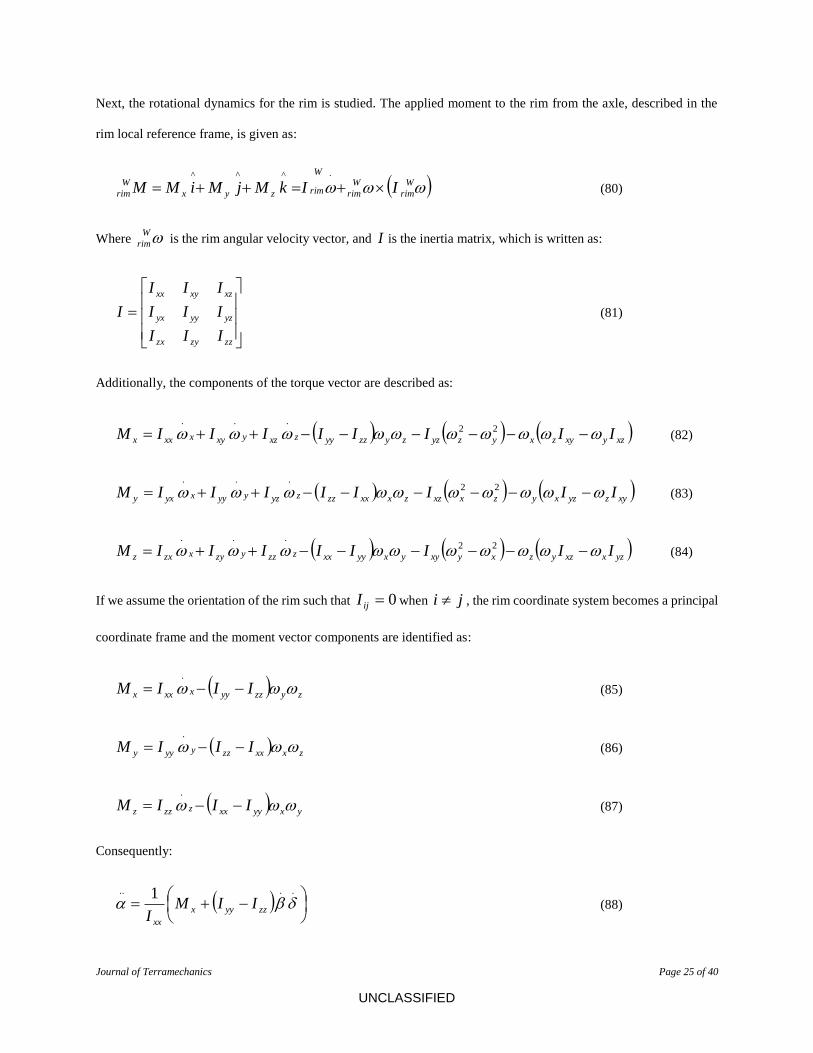
Next, the rotational dynamics for the rim is studied. The applied moment to the rim from the axle, described in the

rim local reference frame, is given as:

W

rim

W

rim

W

rimzyx

W

rim IIkMjMiMM ^^^

(80)

Where W

rim is the rim angular velocity vector, and I is the inertia matrix, which is written as:

zzzyzx

yzyyyx

xzxyxx

III

III

III

I (81)

Additionally, the components of the torque vector are described as:

xzyxyzxyzyzzyzzyyzxzyxyxxxx IIIIIIIIM 22...

(82)

xyzyzxyzxxzzxxxzzzyzyyyxyxy IIIIIIIIM 22...

(83)

yzxxzyzxyxyyxyyxxzzzyzyxzxz IIIIIIIIM 22...

(84)

If we assume the orientation of the rim such that 0ijI when ji , the rim coordinate system becomes a principal

coordinate frame and the moment vector components are identified as:

zyzzyyxxxx IIIM .

(85)

zxxxzzyyyy IIIM .

(86)

yxyyxxzzzz IIIM .

(87)

Consequently:

.... 1 zzyyx

xx

IIMI

(88)


UNCLASSIFIED

.... 1 xxzzy

yy

IIMI

(89)

.... 1 yyxxz

zz

IIMI

(90)

The equations for the sidewall moments that exist between the belts segments and the rim are expressed in the

wheel local reference frame. In order to express these equations in the global reference frame, the following

transformation matrix is used:

tZtXtZrim RRRtR ,,, (91)

It should be noted that the transformation matrix in (91) is a function of time, and is recalculated at every time

step based on the spatial orientation of the rim. The final moment vector at the spindle form the tire sidewall, expressed

in global reference frame is calculated as:

iB

sidewallrim

iG

sidewall MtRM (92)

Where MB

sidewall is the sum of individual torque vectors applied by the belt segments to the tire:

segbeltN

i

iB

sidewall

B

spindle MM_

1

(93)

5 Tire model parameterization

The tire model parameterization is defined as the set of experiments and data processing methods that are

performed to acquire the input parameters for the tire model simulation. There are different methods that can be used

for tire parameterization. These methods range from completely empirical to semi-empirical methods. For the model

developed in this study a complete set of tire parameterization methods for individual parameters is proposed. In

Figure 4, the types of parameters that can be obtained from each set of tests are shown.


UNCLASSIFIED

Figure. 4 - Tire parameterization procedures which are used for defining the tire model parameters (gray

rectangles), and tire parameters resulted from post-processing of each set of tests (light blue rectangles).

In the tire model developed in this study, the stiffness and the damping characteristics of the tire are considered

to be different for in-plane and out-of-plane directions. As a result, during the loading of the tire in the vertical

direction, for example, the slope of the tangent line to the loading-deflection curve is not just due to the in-plane radial

stiffness of the tire. Therefore, for measuring different stiffness and damping parameters of the model, depending

solely on standard measurement procedures is not always effective. Furthermore, conducting a wide variety of tests

on the tire in different configuration, such as axial and tangential loading, tire relaxation time measurements, and cleat

tests requires a large amount of time and resources, which may not always feasible.

Having these limitations in mind, a finite element model (FEM) of the tire has been implemented [14, 15], which

can be used for simulating virtual parameterization tests, as well as for the validation of the lumped mass soft-soil tire

model simulations. As mentioned previously, the tire tread is not considered in the initial version of the FEM model

to make the validation of the lumped mass model easier. Some material properties of the FEM model were obtained

from the manufacturer documentation; the rest of the required properties were obtained through experimental tests

done on a similar tire by other researchers [24]. The FEM model validation based on Tire Model Performance Test

(TMPT) data is done qualitatively and quantitatively. The details of the TMPT program will be explained in the


UNCLASSIFIED

“Experimental study” section. In the qualitative method, the trend of the data with different parameter changes is

studied. The quantitative approach compares measured data from two similar simulations done with different methods.

The finite element model is initially compared with steady-state experimental data. In this regard, the modal analysis

test is performed in order to extract tire mode shapes and associated natural frequency and damping values. The

schematic of the test rig which is used for conducting the modal analysis experiments on the tire is illustrated in Figure

5.

Figure. 5 - The modal analysis test rig used for extracting the tire natural frequencies and damping values.

These values are used accordingly to parameterize the tire material model.

The natural frequencies and damping values for the radial modes (R) and transverse modes (T) of the unloaded,

non-rotating tire are compared to the experimental values obtained from the TMPT data. The results are shown in

Table 1.

Table 1. Comparison between modal analysis simulation test results and experimental data.

Natural Freq. (Hz) Damping %

Modes ABAQUS Test Error ABAQUS Test Error

T0 47.54 47.20 0.72 0.023 0.021 9.52

T1 55.85 61.40 9.04 0.031 0.029 6.9

R0 79.35 81.77 2.96 0.066 0.068 2.94

R1 87.60 97.35 10.01 0.041 0.044 6.82

T2 104.68 116.02 9.77 0.038 0.036 5.56

R2 124.74 122.93 1.47 0.027 0.032 15.63

R3 145.17 149.47 2.87 0.02 0.024 16.67

R4 165.48 176.64 6.31 0.021 0.024 12.5


UNCLASSIFIED

It can be seen that in most of the modes, the FEM model results correlate with the experimental data within a

reasonable error margin. Meanwhile, the model slightly underestimates most of the natural frequencies and radial

damping values; on the other hand, it overestimates the transverse damping values. The natural frequencies and

damping values are further processed in order to find the force elements, stiffness and damping values in different

directions (lateral, radial, longitudinal, inner element, etc.).

Additionally, the dynamic loading radius of the tire is measured using the optical distance measuring sensors

implemented inside the tire. Footprint of the tire on a flat rough surface is measured through pressure pads, and the

stiffness of the tire in radial direction is obtained from tests for which the tire is loaded using hydraulic shakers and

vertical reaction forces are measured through the force hub at the tire spindle in the Terramechanics rig [40]. The

configuration of the test rig and the design of experiment procedures are presented in a separate publication [41].

6 Tire-terrain interaction

Once the tire structure and tire material properties are modeled and implemented in a mathematical framework,

the interface between the model and road surface should be established. This interface searches for the nodal points

that are close to the ground (contact search algorithm), and once the contact is detected the algorithm applies the

required contact condition (contact interface algorithm). The detailed description of the tire-terrain interaction model

is outside the scope of this paper, and is presented in the companion paper [5].

7 Results and discussion

In this section initially we start with a benchmark simulation that demonstrate the dynamic capabilities of the

HSSTM model. As it was explained in the tire-terrain interaction section, when the tire is traveling over the terrain,

the ground under the contact patch gets deformed. If, for the second time, another tire travels on the same path, it will

experience a different amount of resistance from the ground. Furthermore, the elastic and plastic deformation of the

terrain would differ during loading and unloading. To visualize this behavior, the deformation of the ground (sandy

loam) after two consecutive tire passes is illustrated in Figure 6.


UNCLASSIFIED

Figure. 6 - Simulation visualization for the multi-pass effect of a sandy loam terrain.

In this simulation, the tire starts traveling over the terrain in a straight line, and deforms the terrain surface,

creating a rut. Next, the tire continues on a second path, which is perpendicular to the first path. Because the HSSTM

is a nonlinear system, the tire elements go under different states of normal and tangential stresses. As a result, the

permanent plastic deformation of the ground after the tire passage is uneven. This deformation has larger value at the

crossing section of two paths, which has gone through deformation twice. However, this deformation is less than twice

the value of the rut depth on the soil sections negotiated over only once. The mechanical properties of the mineral

terrain which is used for conducting this simulation is same as the Medium terrain shown in Table 2.

When the tire is moving on a deformable terrain under an applied torque at its spindle, the positive shear forces

keep pushing the tire forward, while the negative ground forces (rolling resistance, bulldozing force, etc.) resist the

tire motion. The resultant force is called the drawbar pull, which is an indication for the ability of a vehicle to pull/push

external load, accelerate, or overcome the grade resistance. Consequently, in calculation of the drawbar pull, both

motion resistance due to tire flexing and the one due to soil compaction are included. To normalize this parameter, it

is divided by the normal load at the spindle, thus obtaining the drawbar pull coefficient. The drawbar pull coefficient

explicitly relates the tire tractive performance to the wheel slip ratio and implicitly to the terrain normal and shearing

characteristics. Using the developed model, the drawbar pull coefficient is calculated at four slip ratio values and on

three selective terrain types, which are called soft, medium, and hard soils. The slip ratio is calculated by normalizing

the wheel slip velocity with the carriage longitudinal velocity:


UNCLASSIFIED

100100

xcarriage

xcarriageeff

xcarriage

sxwheel

V

VR

V

V (94)

Where effR is the wheel effective rolling radius and is the wheel rotational velocity. The slip ratio values are

maintained at their nominal values using a PID controller that regulates the applied torque to the spindle. The terrain

mechanical properties used for the simulated terrains are documented in Table 2.

TABLE 2 – Mechanical properties of three mineral terrains used for simulations.

Bekker’s equation Moisture content

(%)

Shear characteristics

Soil Type n

cK

1nm

kN

K

1nm

kN

RS

s

cm

C

1nm

kN

Φ deg

K

Soft terrain (LETE soil)

0.611 1.16 475.0 0 2.5 1.15 31.5 -

Medium terrain (Upland sandy

loam) 0.74 26.8 1522 44.3 2.5 2.7 26.1 0.45

Hard soil (Grenville loam)

1.01 0.06 5880 24.1 2.5 3.1 29.8 0.40

The results of this simulation that indicate the effect of the terrain properties on the mobility performance of the tire

are presented in the Figure 7.

It was observed that increasing the stiffness of the terrain could increase the peak of the drawbar pull coefficient

in addition to its asymptotic value at high slip ratios. The difference between the drawbar pull coefficient on the hard

and medium soils decreases drastically with increasing the slip ratio. This is expected to be a direct effect of the K

parameter variations. As it was discussed earlier, K is the shear deformation parameter and is a measurement of the

magnitude of the shear displacement required for developing the maximum shear stress in the soil. The low slip ratio

region is highly affected by the shear deformation parameter K , whereas the high slip ratio region is almost

insensitive to the its variations [42]. Therefore, the hard soil, with a lower K value, shows higher drawbar pull

coefficients at low slip values, and the difference attenuates by approaching the high slip ratio region. An analogous

trend for the drawbar pull values measured on the similar terrains was reported by other researchers [26].


UNCLASSIFIED

Figure. 7 - Tractive performance of the buffed tire simulated at four slip ratios and three different soil

conditions.

In order to characterize the configuration of the test rig in the simulation environment, an application platform is

designed in order to accommodate the communications with the multibody dynamics solver. The spindle carriage is

represented using a quarter car model, and is implemented in a separate module, which has its own ODE solver. At

every time step, the vehicle model, which is described in a multibody dynamics framework, provides the wheel

kinetics and kinematics variables to the tire model. The time step for the tire model solver is chosen as half the time

step set for the multibody dynamics solver. This is due to the fact that extra calculations are performed in the middle

of the fixed time intervals to improve the accuracy. These extra calculation results are provided to the external solver

for maximizing the ODE solver performance. Next, the tire model updates the position and velocity state vectors of

the tire. Using this new tire configuration, the terrain model exploits the contact conditions, which results in the

tire/ground deflection and stress distribution in the contact patch. The normal and shear stress fields are feedback to

the tire model, which are used for solving the tire equations of motion. At the end of this step, the tire model calculates

three forces and moments at the spindle and feeds them back to the vehicle model. An overview of the discussed

procedure is shown in Figure 8. It should be noted that a great attention is given to the optimization of the tire model

performance in order to make it a practical option for full vehicle simulations. This has become possible by applying

some parallelization and multi-processing techniques to the architecture of the program. Additionally, as for the tire-

vehicle interface, the data communication routines are developed such that they follow the standard formats from

Standard Tire Interface (STI) practices.


UNCLASSIFIED

Figure. 8 - The communication data flow between the tire model modules during the full vehicle simulation.

The vehicle handling and rollover behavior are directly affected by the force and moments at the wheel spindle.

In this regard, the longitudinal force, the lateral force, and the aligning moment values are the quantities of interest

because they define the planar motion of the vehicle. In order to validate the developed model based on these system

response quantities, a straight line driving maneuver is designed. In this test, the tire carriage is moved with the

constant longitudinal speed of 0.5 m/s while a normal force of 4,000 N is maintained at the spindle. Meanwhile, the

applied driving torque at the spindle is increased with a constant rate to allow the wheel slip ratio changes from 0 %

to 60 %. All the forces and moments are measured at the spindle, and the wheel sinkage is calculated using a novel

method developed by Naranjo [33]. In this method, the wheel sinkage is calculated by post-processing the data from

the sensors that are implemented inside the tire cavity. These sensors are integrated units composed of a position

sensitive detector (PSD), five infrared emitting diodes (IREDs), and a signal processing circuit. The similar test

configuration is designed using the developed tire model platform, and simulation runs are conducted at the input

conditions identical to the experimental test setup. The tire used for conducting the tests is a P225/60R16 97S Radial

Reference Test Tire from Michelin. The tire tread is buffed in order to study the performance of the treadles tire.

The validation of the tire model response quantities versus the measurement data is done using the cross plot

validation charts. For every parameter, simulation results are plotted versus the test data across the entire simulation

time span. Next, a linear line is curve-fitted to the resulted data points, and is plotted on the same figure. The validation

results for four main response quantities, including sinkage, longitudinal force, lateral force, and aligning moment are

shown in Figures 9 to 12. The ideal case would be for all the data points to line up on the green curve-fitted line and

for this line to match the 1:1 red dash line. However, due to errors such as measurement errors, modeling errors, and

parameterization errors, this ideal situation is almost impossible to achieve. To assess the quality of the match, curve-

fitted line properties including the slope, intersection with the Y axis and coefficient of determination (2R ) are shown


UNCLASSIFIED

on the figures. For a perfect match, two main parameters of interest, which are the line slope and the 2R index would

be equal to one. The2R index is an indication of how the data is distributed around the curve-fitted line; so, for a

completely scattered data, this value will become zero.

Figure. 9 - System response quantities cross-plot validation: wheel sinkage

Looking at the sinkage and the longitudinal force validation plots suggests that the HSSTM model can do a good

job in estimating these parameters. The solid green curve-fitted line in the sinkage plot starts to deviate from the 1:1

line as the sinkage increases, and always remains below the red dashed line. This means that at higher sinkage values,

the measured sinkage value is greater than the simulation results. The higher sinkage values occur at higher slip values,

at which the tire starts to displace large volumes of soil particles and dig into the terrain. Considering the fact that the

soil volume displacement model is not used in this simulation can justify the trend of the sinkage cross-plot results.

As for the longitudinal force, the model represent a good performance in estimating the measurement data.


UNCLASSIFIED

Figure. 10 - System response quantities cross-plot validation: longitudinal force at the spindle

As shown in Figures 11 and 12, although the test runs are performed in a straight line, the lateral force and the

aligning moment values change during these maneuvers. This can be explained by considering the following facts: (1)

when the tire is traveling on a solid, non-deformable ground, it produces a lateral force and an aligning moment. This

results from the plysteer and the conicity in the tire construction. The effect of these manufacturing defects is modeled

as a pseudo slip angle (for plysteer) and a pseudo inclination angle (for conicity). The pseudo slip angle and the

inclination angle (camber angle) cause the residual lateral force and aligning moment to appear in the straight line

maneuvers; (2) The ground surface is not fully flat and does not have identical mechanical properties in all directions

(non-isotropic). Therefore, once the tire deforms the terrain, the ground reaction force would not be parallel to the

wheel direction of motion. This inclined reaction force produces a component perpendicular to the wheel plane.

Additionally, when the tire sinks into the ground, soil pressure distribution is applied to the tire sidewalls from the

accumulated soil pile that is displaced out of the tire path. This force is known as bulldozing force, and contributes to

the lateral force and, consequently, to the aligning moment generation. The wheel carriage in the Terramechanics test

rig is located near the right wall of the experimental test rig. Therefore, the soil is piled up near the wall edges, and

produces a pressure gradient on the tire sidewall that shifts the generated lateral force values. This effect can be

observed in the shape of the lateral force cross-plot data points. As shown in Figure 11, most of the blue data points


UNCLASSIFIED

are speeded below the green solid curve-fitted line, which means that model underestimates the lateral force values

throughout the simulation.

Figure. 11 - System response quantities cross-plot validation: lateral force at the spindle

FIG. 12 - System response quantities cross-plot validation: aligning moment at the spindle


UNCLASSIFIED

8 Conclusion

In order to model the dynamic behavior of the tire on soft soil, a lumped mass discretized tire model using Kelvin-

Voigt elements is developed. This model, named HSSTM, is developed to be easily linked with multibody dynamics

software packages to simulate vehicle performance on deformable terrains. To optimize the computational time of the

code, different techniques were used in memory allocation, parameter initialization, code sequence, and multi-

processing. The computational time of the code had a significant improvement relative to previous codes developed

in this institute up to the speed of real time simulations.

The tire parameterization is performed using a reduced finite element tire model for the same tire, modal analysis,

and other experimental test procedures. In the parameterization step sensitivity analysis tools were incorporated in

order to reduce the complexity of the model, and fit more accurate parameters values based on the test data.

Experimental tests were performed on the Terramechanics rig at the Advanced Vehicle Dynamics Laboratory at

Virginia Tech using the P225/60R16 97S Radial Reference Test Tire from Michelin. The tests were performed on

sandy loam, and data were collected for various case studies and parameter changes.

Different case studies were simulated in order to analyze the performance of the developed model. Initially, a soil

multi-pass effect simulation is conducted to demonstrate the functionality of the model. Next, the tire drawbar pull

coefficients on three selective terrains are estimated. It is shown that the drawbar pull coefficients are mainly

influenced by the terrain stiffness and shear deformation parameter. As for the validation case studies, a straight line

driving maneuver is conducted at constant normal load and varying slip ratio values. Using the cross-plot validation

graphs it is shown that the HSSTM can estimate four main vehicle handling parameters including longitudinal force,

lateral force, aligning moment, and sinkage with a reasonable accuracy. The observed discrepancies are thought to be

mainly from the test conditions that are not modeled in the simulations, such as soil displacement at high slip ratios,

tire construction defects (plysteer, comity), and soil bulldozing effect due to the soil compaction near the walls of the

test rig.


UNCLASSIFIED

9 Acknowledgment

This project is funded in part by the Automotive Research Center, a U.S. Army Center of Excellence for Modeling

and Simulation of Ground Vehicles. We want to thank our quad members, Dr. B. Ross from Motion Port and Mr. D.

Christ from Michelin for all of the time and support they have dedicated to us.

10 References

1. Gipser, M., The FTire Tire Model Family. 2003, Esslingen University of Applied Sciences: Esslingen, Germany. p. 18.

2. Oertel, C., On Modeling Contact and Friction Calculation of Tyre Response on Uneven Roads. Vehicle System Dynamics, 1997. 27(S1): p. 289-302.

3. Oertel, C. and A. Fandre. Ride Comfort Simulations and Steps Towards Life Time Calculations: RMOD-K and ADAMS. in International ADAMS User's Conference. 1999. Berlin, Germany.

4. Gallrein, A. and M. Backer, CDTire: A tire model for comfort and durability applications. Vehicle System Dynamics, 2007. 45(1): p. 69-77.

5. Taheri, S., C. Sandu, and S. Taheri, Hybrid Soft Soil Tire Model (HSSTM). Part II: Tire-Terrain Interaction Modeling. Journal of Terramechanics, 2015.

6. Taheri, S., et al., A technical survey on Terramechanics models for tire–terrain interaction used in modeling and simulation of wheeled vehicles. Journal of Terramechanics, 2015. 57: p. 1-22.

7. Pacejka, H.B., and Bakker, E., The Magic Formula Tyre Model. Vehicle System Dynamics, 1992. 21(001): p. 1-18.

8. Pacejka, H.B. and E. Bakker, The Magic Formula Tyre Model. Vehicle System Dynamics, 1992. 21(001): p. 1-18.

9. Chae, S., Nonlinear Finite Element Modeling and Analysis of a Truck Tire, in Intercollege Graduate Program in Materials. 2006, Pennsylvania State University. p. 207.

10. Mastinu, G. and E. Pairana, Parameter Identification and Validation of a Pneumatic Tyre Model. Vehicle System Dynamics, 1992. 21(01): p. 58-81.

11. Kilner, J., Pneumatic tire model for aircraft simulation. Journal of Aircraft, 1982. 19(10): p. 851-857. 12. Madsen, J., et al., A Physics-Based Vehicle/Terrain Interaction Model for Soft Soil Off-Road Vehicle

Simulations. SAE International Journal of Commercial Vehicles, 2012. 5(1): p. 280-290. 13. Negrut, D. and J.S. Freeman, Dynamic tire modeling for application with vehicle simulations

incorporating terrain. SAE transactions, 1994. 103(6): p. 96-103. 14. Taheri, S., Finite Element Modeling of Tire-Terrain Dynamic Interaction for Full Vehicle Simulation

Application in Mechanical Engineering 2014, Virginia Tech Blacksburg, Virginia 15. Taheri, S., C. Sandu, and S. Taheri, Finite Element Modeling of Tire Transient Characteristics in

Dynamic Maneuvers. SAE international Journal of Passenger Cars, 2014. 7(1): p. 9. 16. Chan, B.J., Development of an off-road capable tire model for vehicle dynamics simulations, in

Mechanical Engineering. 2008, Virginia Tech: Blacksburg, VA. p. 226. 17. Chan, B.J. and C. Sandu, Development of a 3-D Quasi-static Tire Model for On-road and Off-road

Vehicle Dynamics Simulations: Part III–Off-road Flexible Wheel Model. International Journal of Vehicle Systems Modelling and Testing, 2014. 9(2): p. 151-176.

18. Chan, B.J. and C. Sandu, Development of a 3-D Quasi-static Tire Model for On-road and Off-road Vehicle Dynamics Simulations: Part II–Off-road Rigid Wheel Model. International Journal of Vehicle Systems Modelling and Testing, May 2014. 9(2): p. 107-136.

19. Chan, B.J. and C. Sandu, Development of a 3-D Quasi-static Tire Model for On-road and Off-road Vehicle Dynamics Simulations: Part I–On-road Flexible Tire Model. International Journal of Vehicle Systems Modelling and Testing, 2014. 9(1): p. 77-105


UNCLASSIFIED

20. Wong, J.Y. and V.M. Asnani, Study of the correlation between the performances of lunar vehicle wheels predicted by the Nepean wheeled vehicle performance model and test data. Proceedings of the Institution of Mechanical Engineers, Part D: Journal of Automobile Engineering, 2008. 222(11): p. 1939-1954.

21. Bekker, M.G., Introduction to Terrain-Vehicle System. 1969: Ann Arbor: The University of Michigan Press.

22. Bekker, M.G., Off the Road Locomotion. 1960, Ann Arbor, Michigan: University of Michigan Press. 23. Bekker, M.G., The Theory of Land Locomotion. 1956, Ann Arbor, Michigan: University of Michigan

Press. 24. Bekker, M.G., Theory of Land Locomotion : The Mechanics of Vehicle Mobility. 1956: Ann Arbor:

The University of Michigan Press. 25. Wong, J.Y. and J. Preston-Thomas, On the Characterization of the Shear Stress-Displacement

Relationship of Terrain. Journal of Terramechanics, 1983. 19(4): p. 225-234. 26. Wong, J.Y., On The Study of Wheel-Soil Interaction. Journal of Terramechanics, 1984. 21(2): p.

117-131. 27. Wong, J.Y. and A.R. Reece, Prediction of Rigid Wheel Performance Based on the Analysis of Soil-

Wheel Stresses. Part I. Performance of Driven Rigid Wheels. Journal of Terramechanics, 1967. 4(1): p. 81-98.

28. Wong, J.Y. and A.R. Reece, Prediction of Rigid Wheel Performance Based on the Analysis of Soil-Wheel Stresses. Part II. Performance of Towed Rigid Wheels. Journal of Terramechanics, 1967. 4(2): p. 7-25.

29. Teheri, S., et al. Off-road Soft Soil Tire Model. in Presentation for the 7th Americas Regional ISTVS Conference 2013. Tampa, FL.

30. Taheri, S., C. Sandu, and S. Taheri. Development and Implementation of a Hybrid Soft Soil Tire Model (HSSTM). in The 18th International ISTVS Conference Seoul, Korea. 2014.

31. Pinto, E., A Three Dimensional Discretized Tire Model for Soft Soil Applications, in Mechanical Engineering. 2012, Virginia Tech: Blacksburg, VA.

32. Sandu, C., et al. Off-Road Soft Soil Tire Model and Experimental Testing. in Proceedings of the 12th European ISTVS Conference 2012. Pretoria, South Africa.

33. Sandu, C., et al. Off-Road Soft Soil Tire Model Development, Validation, and Interface to Commercial Multibody Dynamics Software. in Proceedings of the 17th International ISTVS Conference 2011. Blacksburg, VA, USA.

34. Umsrithong, A. and C. Sandu, A 3D semi-empirical on-road transient tire model. SAE International Journal of Commercial Vehicles, 2010. 3(1): p. 42-59.

35. Umsrithong, A. and C. Sandu. A 3D semi-empirical stochastic tire model on hard flat and uneven surfaces. in International Congress on Automotive and Transport Engineering. 2010. Brasov, Romania.

36. Umsrithong, A., Deterministic and Stochastic Semi-Empirical Transient Tire Models. 2012, Virginia Tech: Blacksburg, VA.

37. Umsrithong, A. and C. Sandu. Parameter Identification and Experimental Validation of a Discrete Mass Tire Model for Uneven Rigid Terrain. in Proceedings of ASME 2012 IDETC/CIE 14th International Conference on Advance Vehicle Technologies (AVT). 2012. Chicago, IL: American Society of Mechanical Engineers.

38. Umsrithong, A. and C. Sandu, A Semi-Empirical Tire Model for Transient Maneuver of On Road Vehicle, in SAE Commercial Vehicle Engineering Congress and Exposition. 2009: Chicago, IL. p. 9.

39. Umsrithong, A. and C. Sandu, Stochastic transient tyre model for vehicle dynamic simulations on rough rigid ground. International Journal of Vehicle Systems Modelling and Testing, 2012. 7(4): p. 351-371.

40. Dasch, J.M. and D.J. Gorsich, TARDEC Story: Sixty-Five Years of Innovation, 1846-2010. 2012: Defense Department, Army, U.S. Army Tank Automotive Research, Development and Engineering Center (TARDEC).

41. Naranjo, S.D., et al., Experimental testing of an off-road instrumented tire on soft soil. Journal of Terramechanics, 2014. 56: p. 119-137.

42. Wong, J.Y., Terramechanics and Off-Road Vehicle Engineering: Terrain Behaviour, Off-Road Vehicle Performance and Design. 2nd Edition ed. 2010, Amsterdam, The Netherlands: Elsevier.


UNCLASSIFIED

HYBRID SOFT SOIL TIRE MODEL (HSSTM). PART I: TIRE …world situation. In this regard, an...

Documents

Transcript of HYBRID SOFT SOIL TIRE MODEL (HSSTM). PART I: TIRE …world situation. In this regard, an...