Hybrid Lattice-Boltzmann/Level-set Method for Liquid...

Hybrid Lattice-Boltzmann/Level-set Method for Liquid Simulation and Visualization

Youngmin Kwak1*, C.-C. Jay Kuo1, Aiichiro Nakano2

1 Ming-Hsieh Department of Electrical Engineering, University of Southern California Los Angeles, CA 90089

[email protected] [email protected]

2 Department of Computer Science, University of Southern California Los Angeles, CA 90089

[email protected]

Abstract. The particle level set method (PLSM) and the lattice Boltzmann method (LBM) have been two major physics-based liquid simulation techniques used in computer graphics to generate splendid and dynamic visual effects. PLSM suffers from a high computational cost which arises from the global pressure correction step whereas LBM requires a large amount of memory to store distribution functions. In this work, we propose a hybrid lattice Boltzmann method (HLBM), which integrates PLSM and LBM, to visualize realistic liquid motion with emphasis on the behavior of the liquid-gas interface. HLBM first runs the LBM solver, com-putes macroscopic velocities, and extrapolates the velocity field to the gas region. Subsequently, the level set function and particles are advected by the extrapolated velocity field, and advected particles are used to correct errors in the level set function based on PLSM. Finally, the den-sity difference between LBM and PLSM solvers is added to the distribution functions to cor-rect the errors of LBM. We test the method for the broken dam and the water drop simula-tions. The results show that HLBM improves the quality of the fluid simulation without in-creasing the number of grids. Compared to the simulation using LBM with a grid resolution of 350 , the mean of the geometrical distance from the ground truth is 21.70% and 13.02% less using HLBM with the same number of grids, for the water drop and the broken dam simulations,

* Corresponding Author. Email: [email protected].

International Journal of Computational Science

1992-6669 (Print) 1992-6677 (Online) www.gip.hk/ijcs

© 2009 Global Information Publisher (H.K) Co., Ltd.

All rights reserved.

GLOBAL INFORMATION PUBLISHER 1

respectively. The simulation results also show that HLBM offers more splashy and dynamic visual effects than LBM without increasing the grid size.

Keywords: lattice Boltzmann method, hybrid lattice Boltzmann method, level set method, particle level set method, fluid/liquid simulation, physics-based fluid simulation.

1 Introduction

Realistic liquid simulation is important for providing splendid and dynamic visual effects in computer games and special effects in movies. The physics-based approach approximates the laws of phys-ics by numerical algorithms and creates realistic and plausible motion of animated liquids automati-cally. It is more accurate than non-physics-based approaches because it generates complete infor-mation and has the ability to simulate realistic and ideal conditions [1]. It is also easy to incorpo-rate control mechanisms such as user interaction with the physics-based approach. Thus, the phys-ics-based approach has recently become the mainstream in liquid simulation.

The level set method (LSM) [2] was used for liquid simulation based on the Navier-Stokes equa-tions. Later, it was improved by adding particles to correct errors, and the resulting method was called the particle level set method (PLSM) [3]. PLSM is one of the most popular fluid simulation methods because of its realistic and smooth representation of liquids. However, it suffers from the high computational complexity of solving the Poisson equation needed in the global pressure correc-tion step to keep the velocity field divergence free[4]. Another liquid-simulation method is the lattice Boltzmann method (LBM), which originated from lattice gas cellular automata [5]. LBM provides a first-order explicit discretization of the Boltzmann equation in a discrete phase-space. The simu-lation region of LBM is divided into a Cartesian grid of cells, each of which only interacts with cells of its direct neighborhood. In contrast, PLSM demands interaction of all cells in the global pressure correction step. Generally speaking, LBM is simpler and faster than PLSM with two shortcomings: 1) it demands more memory to store distribution functions, and 2) it has tight time step restrictions.

In this paper, we propose a hybrid lattice Boltzmann method (HLBM) that integrates LBM and PLSM to visualize realistic liquid motion with emphasis on the behavior of the liquid-gas interface. HLBM enables faster liquid simulation compared to PLSM because the global pressure correction step is not required, and requires less memory space compared to LBM because HLBM improves the quality of the liquid simulation without increasing the grid size. Experimental results showed that HLBM improves the quality of the fluid simulation without increasing the number of grids. Specifically, we test HLBM for the broken dam and the water drop simulations.The results show that HLBM improves the quality of the fluid simulation without increasing the number of grids at the expense of the slightly higher computational cost. Compared with the simulation using LBM with a grid resolution of 350 , the mean of the geometrical distance from the ground truth has been decreased by 21.70% and 13.02% for the water drop and the broken dam simulations, respectively, using HLBM with the same number of grids. The simulation results also show that HLBM offers


GLOBAL INFORMATION PUBLISHER2

more splashy and dynamic visual effects than LBM without increasing the grid size. As mentioned before, LBM demands a larger memory space to store distribution functions. Thus, it is not suitable for a high quality liquid simulation with large grid size. However, HLBM improves the quality of the liquid simulation without increasing the grid size at the expense of the slightly higher computational cost. Thus, HLBM is suitable for a high quality liquid simulation with less memory space than LBM.

The rest of the paper is organized as follows. In Section 2, both LBM and PLSM are described along with their basic algorithm. The proposed HLBM is detailed in Section 3. Simulation results are presented in Section 4. Finally, concluding remarks are given in Section 5.

2 Lattice Boltzmann and Particle Level Set Methods

2.1 Lattice Boltzmann Method!

The Boltzmann equation [6] is a subject in statistical physics that describes the behavior of a gas on a microscopic scale. The Boltzmann equation with the Bhatnagar-Gross-Krook (BGK) collision approximation [7] can be written as

1 ( )f f f gt

!"

# + $% = & & ,#

(1)

where ( )f f t!= , ,x is the single-particle distribution function, ! is the microscopic velocity, " is the relaxation time due to collision, and g is the Boltzmann-Maxwell distribution function. Dis-cretizing time and phase space, Eq. (1) can be rewritten as

( ) ( )( ) ( )

eqi i

i i if t f tf t t f t

', & ,+ , + = , & ,x xx e x x! ! (2)

where t! and x! represent the time and the spatial step sizes, respectively. ( )eqif t,x is the equi-

librium distribution function used to represent a stationary state of the fluid. The rate of change toward equilibrium is 1 '/ , the inverse of the relaxation time, and it is chosen to produce the de-sired value of fluid viscosity. The equilibrium distribution function can be derived using the Tay-lor expansion of the Maxwell distribution [8]. The Navier-Stokes equations can be derived from the Boltzmann equation by a multi-scale analysis called the Chapman-Enskog expansion when the Knudsen number is smaller than one [9,10].

The basic algorithm of LBM consists of two steps: the streaming step and the collision step [11]. These are usually applied in association with no-slip boundary conditions in domain boundaries or obstacles. Also, the free surface boundary condition is adopted in the simulation of the two phase flow. LBM restricts the particle movement to a limited number of directions. A three dimensional model with 19 velocities, which is commonly denoted by D3Q19, will be used in this paper.



Fig. 1. Illustration of the streaming step and the collision step for a fluid cell proposed by Thürey[12]

The D3Q19 model has 19 velocity vectors 1 19( )..e with length 0 1( )e , length 1 2 7( )..e , and length

8 192( )...e Each velocity vector has its own floating point distribution function, if , which repre-sents the fraction of particles moving with velocity ie . Thus, in the D3Q19 model, there are parti-cles not moving at all 1( ),f moving with speed 1 2 7( ),f .. and moving with speed 8 192( ).f ..

During the streaming step, all distribution functions (DFs) are advected with their respective velocities. This results in a movement of the floating point value to the neighboring cells as shown in Fig. 1 from [12]. Formulated in terms of DFs, the streaming step can be written as

( ) ( )i i if t t f x t( , + = & , ,x x e! ! (3)

where x! is the size of a cell and t! is the time step-size. The streaming step alone is not enough to simulate the behavior of an incompressible fluid, since it

is governed by the on-going collision of particles with each other as well. The collision step accounts for this by weighting DFs of a cell with eq

if . The equilibrium DFs represent a stationary state of the fluid. They depend on the density and the velocity of the fluid, which are computed by the summa-tion of all DFs in one cell from the incompressible model of [13] as

andi i if f) = , = .! !u e (4)

The collision of molecules in a real fluid is approximated by linearly relaxing the DFs of a cell towards their equilibrium state. Thus, each if is weighted with the corresponding eq

if as

( ) (1 ) ( ) eqi if t t w f t t wf(, + = & , + + ,x x! ! (5)

where w is a parameter that controls the viscosity of the fluid. Fig. 1 illustrates the streaming and collision steps for a fluid cell proposed by Th u"" rey[14]. Values computed by Eq. (5) are stored as DFs for time t t+! . Since each cell needs the DFs of its adjacent cells from the previous time step,



two arrays for DFs (i.e., the current and the last time steps) are usually used. Thus, LBM requires a large amount of memory to store those floating point DFs.

To model the solid-liquid interface, we implement the no-slip boundary condition by applying the link bounce back rule that results in the placement of the boundary halfway between the fluid and obstacle cells [14]. If the neighboring cell at ( )it+x e! is an obstacle cell during streaming, the DF from the inverse direction of the current cell is used. That is, we change Eq. (3) to

( ) ( )i if t t f t( , + = , ,x x#! (6)

where the subscript of i# denotes the value for the inverse direction of a value with subscript i. Simulation of free surfaces demands a distinction between regions that contain fluid and re-

gions that contain only gas. This is done by marking cells that contain no fluid as empty in the flag field. As with obstacle cells, the DFs of these cells are completely ignored in the simulation. How-ever, in contrast to boundary cells, the fluid might move into this empty area at some point in the simulation. To track the fluid motion, another cell type is introduced, which is called the interface cell. These cells form a closed layer between fluid and empty cells. Then, we can track mass ex-change between the interface and gas cells. Furthermore, the mass of a cell, which is calculated for the next time step, is used to update the cell type [12,15].

2.2 Level Set Method!

The level set (LS) is an implicit function to construct the surface between fluids, which has the characteristics of the signed distance function. The level set method (LSM) was introduced to the computer graphics community by Osher and Fedkiw [2]. LSM discretizes the Navier-Stokes equa-tions (NSEs) and tracks interfaces during simulation. NSEs for incompressible fluids can be de-scribed by

0% $ = ,u (7)

and

$$

$2 1( ) ,

diffusion forceadvectionpressure

p ft

*)

# = & $% + % & % +#u u u u%&'&( (8)

where u , p , * and ) represent the velocity, pressure, viscosity coefficient and density of flu-ids, respectively, and f is an external force, such as the gravitational force. Eq. (7) is called the continuity equation because the velocity field of incompressible fluids is divergence free. Eq. (8) is the momentum conservation equation consisting of four terms: advection, diffusion, pressure and force [16]. To make the velocity field divergence free, we have to solve the Poisson equation with the Neumann boundary condition over the entire computational domain [4]. The Poisson equation becomes a sparse linear system when spatially discretized, and it can be solved using the precondi-tioned conjugate gradient method, which incurs a large computational cost.



The level set function, + , evolves by an externally given velocity field, u , which is obtained by the numerical solution to the NSEs. The evolution equation of the level set function is called the level set equation, which can be written as

0t+ ++ $% = .u (9)

Eq. (9) can be spatially discretized using the 5th order accurate Hamilton-Jacobi weighted essen-tially non-oscillatory (HJ-WENO) scheme [17] and temporally discretized using the 3rd order total variation diminishing Runge-Kutta (TVD-RK) scheme as done in [3].

Generally speaking, LSM enables a smooth surface representation because of the nature of the level set function. However, the volume of liquid decreases severely during simulation.

2.3 Particle Level Set Method!

The particle level set method (PLSM) was proposed by Enright et al. [3] to overcome the volume loss problem of LSM. PLSM is a thickened front tracking algorithm that uses massless marker particles to assist LSM in tracking flow characteristics in under-resolved regions around the inter-face. Particles are labeled by the corresponding level set values with the positive or the negative sign. Positive particles are located in the band near the interface which has positive level set func-tion values. Negative particles are located in the band near the interface which has negative level set function values. Those particles work to correct errors of the level set functions by comparing the level set functions from escaped particles and grid points [3].

To keep the level set function as a signed distance function in simulation, the fast marching method (FMM), which systemically advances the front in an upwind fashion, is used because of its simplicity and efficiency [18]. FMM is also used for velocity extrapolation, which extends the velocity to grid points around the interface, to avoid the introduction of any discontinuities in the speed close to the interface [19].

3 Hybrid Lattice Boltzmann Method

As explained in Section 2.2, liquid simulation using LSM enables smooth surface representation but it suffers from a huge computational cost because of the global pressure correction step to solve the Poisson equation for the entire computational domain. On the other hand, liquid simulation using LBM has an efficient basic algorithm and preserves mass as discussed in Section 2.1. However, it suffers from a small time step restriction and a high memory requirement [12]. In this section, we propose a hybrid algorithm that integrates LBM with PLSM for more realistic and faster liquid simulation.

To combine LBM with PLSM, we first need to find the macroscopic velocity field to advect the level set function and particles. The macroscopic velocity of each cell can be calculated using Eq. (4) and the distance from the center of each cell to the fluid interface can be calculated using



the marching cube algorithm [20]. Thus, the level set function can be advected using the macro-scopic velocity field. And the semi-Lagrangian advection scheme [16] is used for the advection method. However, the macroscopic velocities of a lattice cell can be calculated only for fluid and interface cells. In other words, the velocities of a gas cell are always zero using Eq. (4) because the distribution functions at x , ( )if x , are all zero. As the level set functions have to be defined in both the gas and fluid regions, velocities from the fluid have to be extrapolated into the gas region with the fast marching method as described in Section 2.3.

Table 1. Multi-resolution density calculation up to 3rd level for the PLSM part. Here, we use F, IF, and G to denote fluid, interface, and gas cells, respectively, and ) is density of the current (sub) cell

step 1 If current cell is F, 1) =

Else if current cell is G, 0) =

Else if current cell is IF, split the cell into 34 sub-cells

1cm and check whether the sub-cell is F, G, or, IF

step 2 If current sub-cell is F, 31 4) = /

Else if current sub-cell is G, 0) =

Else if current sub-cell is IF, split the sub-cell into 34 sub-sub-cells

1cm and check whether the sub-sub-cell is F, G, or, IF

step 3 If current sub-sub-cell is F, 61 4) = /

Else if current sub-sub-cell is G, 0) =

Else if current sub-sub-cell is IF, 61 2 1 4) = / , /

step 4 Find the sum of ) for entire cell

Fig. 2. Multi-resolution density calculation up to 3rd level, where the left figure shows the original profile of cells and the right figure shows the multi-resolution density calculation. Symbols F, IF, and G denote fluid, interface, and gas cells, respectively



The hybrid lattice Boltzmann method (HLBM) is described below.

– Step 1: Run the LBM solver, where the streaming and the collision steps are performed using Eq. (3) and Eq. (5), respectively. The obstacle and free surface boundary conditions are also ap-plied, and the distribution functions of the next time step, ( )if t t, + -x , for each lattice are cal-culated.

– Step 2: Calculate Macroscopic velocities for the current time step, ( )t,u x , using Eq. (4). – Step 3: Extrapolate the velocity field, ( )t,u x , to the gas region because LBM does not have

velocities for the gas region. This extrapolated velocity field, ( )ext t,u x , is required for the ad-vection of PLSM because the semi-Lagrangian advection scheme needs velocities of the gas region along with velocities of the liquid region.

– Step 4: Advect the level set function, ( )t+ ,x , and particles, ( )k tp , by the extrapolated velocity field, which is calculated in the previous step. The level set function are advected using the semi-Lagrangian advection scheme and particles are advected using the 3rd order TVD-RK method.

– Step 5: Correct errors of the level set function using advected particles in PLSM. – Step 6: Calculate two different density fields obtained from the LBM and the PLSM solvers.

For the LBM part, the density of each cell, LB) , can be calculated by the sum of distribution functions using Eq. (4). For the PLSM part, the density of each cell, PLS) , is calculated using multi-resolution density calculation scheme up to 3rd level as described in Table 1. Fig. 2 also shows 2D example of the density calculation method.

– Step 7: Add the density difference between the LBM and the PLSM solvers to distribution functions to correct errors of LBM as

Fig. 3. Overview of the hybrid lattice Boltzmann method, where the dotted box (green) represents the over-view of LBM only. In next time step, ( )HLBM

if t t, + -x is used as an input distribution function instead of ( )if t t, + -x



( ) ( )

( ) ( )HLBM PLS LBi i

t t t tf t t f t t

M) ), + - & , + -, + - = , + - + ,x x

x x (10)

– where if and HLBMif represent distribution functions from LBM and HLBM, respectively. In

Eq. (10), LB) and PLS) are densities calculated from LBM and PLSM, respectively. Note that M is equal to 19 for the 3 19D Q model. Fig. 3 shows a schematic overview of the HBLM algorithm, where ( )k tp represents the particle

with id k at time t. In the next time step, ( )HLBMif t t, + -x is used as an input distribution function

instead of ( )if t t, + -x .

4 Simulation Results

For fluid animation, the Boltzmann equation needs to be solved numerically using a system called the fluid solver. We use the El’Beem solver, a free surface fluid solver based on LBM, for this purpose [21]. For the hybrid LBM (HLBM) solver, we added PLSM modules such as level set functions, particles, velocity extrapolation, and error correction to the El’Beem solver. After run-ning the HLBM solver, we get binary obj files which can be imported to Blender [22], a free open source 3D content creation suite. Blender can modify material properties such as color, and render the scene using its internal rendering engine. Simulation results in this paper were obtained using a PC with a 2.2GHz CPU and 4GB RAM..

Fig. 4 shows 4 frames from the broken dam simulation using LBM (the top row) and HLBM (the bottom row). Both LBM and HLBM were run with a resolution of 350 with real world size 0 1 m. , 50 frames/sec, and the no-slip boundary condition. For each frame using LBM, the fluid solver and surface generation took 20 seconds and the rendering of the 600 600, image took 80 seconds. For the simulation of HLBM, we used 64 particles for each cell with 6 x+| |< ! as an initial condition. The fluid solver and surface generation took 24 seconds and the rendering of the 600 600, image took 85 seconds for each frame using the internal raytracing renderer in Blender. Thus, the simulation time using HLBM was about 20 % longer than LBM.

Fig. 5 shows 4 frames from the water drop simulation using LBM (the top row) and HLBM (the bottom row). Both cases were run with a grid resolution of 350 with real world size 0 1 ,m. 50 frames/ sec, and under the no-slip boundary condition. LBM took about 22 seconds for the fluid solver and surface generation and 91 seconds to render each frame to the 600 600, image. HBLM took 25 seconds for the fluid solver and surface generation and rendering took 95 seconds per frame. The simulation time of HLBM is 13.6 % higher than LBM..

As we see from Figs. 4 and 5 however, the visual quality of the simulations is improved using HLBM at the expense of a little bit higher computational cost. In particular, HLBM enables a more splashy effect because the resolution of the fluid simulation is increased by adding particles.



Fig. 4. The broken dam simulation using LBM (the top row) and HLBM ( the bottom row) with a resolution of 350 . The columns from the left to the right represent the 1 ,st the 6 ,th the 11 ,th and the 16th frames, respectively

Fig. 5. The water drop simulation using LBM (the top row) and HLBM (the bottom row) with a resolution of 350 . The columns from the right to the left represent the 1 ,st the 6 ,th the 11 ,th and the 16th frames,

respectively

Fig. 6 shows the 11th frame of the broken dam simulation using LBM (the upper left) and HLBM (the upper right), and the 17th frame of the water drop simulation using LBM (the lower left) and HLBM (the lower right). For the broken dam simulation, we see a more splashy effect of HLBM at the right wall of the image. This splashy effect is also present at the water drop simulation, espe-cially at the center of the image. Also, the liquid surface has finer detail with HLBM than that with LBM.



Fig. 6. The 11th frame of the broken dam simulation using LBM (the upper left) and HLBM (the upper right) and the 17th frame of the water drop simulation using LBM (the lower left) and HLBM (the lower right)

To quantify the visual improvement of HLBM over LBM, we first obtained the ground truth for the broken dam and the water drop examples using LBM with a very high resolution grid (i.e.,

3150 ) and the same initial and boundary conditions. Then, we got simulation results using LBM and HLBM with grids of a lower resolution. They include: LBM with a resolution of 350 , LBM with a resolution of 360 , LBM with a resolution of 364 , and HLBM with a resolution of 350 . Finally, we used MeshDev [23] to compare the geometric distances between the computed results and their ground truth values.

The mean and the variance of the geometrical distances are given in Table 2 and Table 3, re-spectively. Based on the data in Table 2, we plot the mean of the geometrical error as a function of the frame number in Figs. 7 for the broken dam and water drop cases, respectively. We have the following observations. – For the water drop case, the geometrical distance is significantly larger at the 16th frame com-

pared to other frames since this is a very splashy frame. Similarly, for the broken dam case, the 31st frame is a splashy frame and it also has a larger geometrical distance than other frames. Thus, we conclude that the error becomes larger for splashier frames.



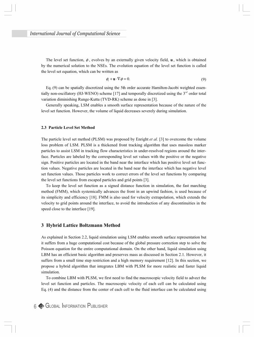
– For the broken dam case, the mean error of HLBM with a grid resolution of 350 is 13.02% lower than that of LBM with a grid resolution of 350 , and 0.96% lower than that of LBM with a grid resolution of 360 . HLBM with a resolution of 350 performs almost the same as LBM with a resolution of 360 .

– For the water drop case, the mean error of HLBM with a resolution of 350 is 21.70% lower than that of LBM with a resolution of 350 , but 6.95% higher than that of LBM with a grid resolution of 360 . One reason for the performance difference between the broken dam and the water drop cases

could be that the water drop case has a splashier effect than the broken dam case, which lowers the accuracy of the calculation of the mean error using MeshDev.

Table. 2. The mean of the geometrical distance to the ground truth, where results were obtained using LBM with a grid resolution of 350 , LBM with a grid resolution of 360 , LBM with a grid resolution of

364 , and HLBM with a grid resolution of 350 and geometrical distances were calculated for every fifth frame

frame number 1 6 11 16 21 26 31 36 41

broken dam LBM 350 1.3905 1.3983 1.3958 1.3853 1.8460 1.8010 1.8129 1.5937 1.3257

broken dam LBM 360 0.8951 0.9615 1.3301 1.2225 1.5318 1.5781 1.8747 1.4580 1.3989

broken dam LBM 364 0.8075 0.8977 1.1926 1.0811 1.4502 1.5414 1.6588 1.5370 1.2923

broken dam HLBM 350 1.0595 1.0957 1.1883 1.1699 1.5155 1.5584 1.7826 1.5315 1.2318

water drop LBM 350 1.9095 1.9687 1.8346 2.0708 1.8280 1.9787 1.9620 1.9264 1.9271

water drop LBM 360 1.2617 1.4168 1.3258 1.7971 1.4298 1.4253 1.3824 1.3462 1.3581

water drop LBM 364 1.1299 1.1837 1.0890 1.3264 1.3137 1.2559 1.2067 1.1423 1.1450

water drop HLBM 350 1.4388 1.5026 1.3983 1.9262 1.4577 1.4862 1.4888 1.4507 1.4789

Table 3. The variance of the geometrical distance to the ground truth, where results were obtained using LBM with a resolution of 350 , LBM with a resolution of 360 , LBM with a resolution of 364 , and HLBM with a resolution of 350 , and geometrical distances are calculated for every fifth frame

frame number 1 6 11 16 21 26 31 36 41

broken dam LBM 350 0.8071 1.0939 0.9880 1.0442 1.8604 1.9892 2.3704 1.9391 1.0136

broken dam LBM 360 0.3840 0.5090 1.0040 0.8678 1.3458 1.8347 3.6313 1.6073 1.2040

broken dam LBM 364 0.2716 0.4542 1.2410 0.6734 1.4046 1.8883 2.9675 2.2410 1.1349

broken dam HLBM 350 0.4892 0.6729 0.9241 0.8014 1.4740 1.6775 3.2785 1.9424 0.9815

water drop LBM 350 1.5986 1.7722 1.6713 2.7791 1.4224 1.8309 1.8254 1.8262 1.8622

water drop LBM 360 0.8145 0.8276 0.9576 8.4270 1.3640 1.1492 0.9811 1.0047 1.0170

water drop LBM 364 0.5123 0.5578 0.5955 1.9227 2.8787 1.4572 0.9623 0.7333 0.7101

water drop HLBM 350 0.9064 1.0187 0.9350 9.0859 1.9982 1.0485 1.0499 1.0188 1.0830



As for the computational complexity, the simulation time of LBM with a grid resolution of 360 demands 1.7 times more simulation time than LBM with a grid resolution of 350 . On the other hand, HLBM with a grid resolution of 350 takes about 1.2 times more simulation time than LBM with a grid resolution of 350 . Thus, the proposed HLBM improves the quality of the simulation without increasing the computational cost much.

Fig. 7. The mean of the geometrical error as a function of the frame number for LBM with a grid resolution of 350 (the red line), LBM with a grid resolution of 360 (the green line), LBM with a grid resolution of 364

(the blue line), and HLBM with a grid resolution of 350 (the black line)

5 Conclusion

The PLSM requires a high computational cost to solve the Poisson equation from the global pres-sure correction step. Although LBM is simpler and faster than PLSM, it demands a larger amount of memory. In this work, we integrated LBM and PLSM and derived a new method, called HLBM, to overcome these difficulties. It was shown by experimental results that HLBM can offer a splashy and dynamic visual effect with the aid of PLSM. Furthermore, it can improve the quality of the fluid simulation of LBM without increasing the grid size.

Acknowledgments

The authors would like to thank Martin Gawecki of the University of Southern California for useful comments on the preparation of this article.

References

1. Pijush K. Kundu, Ira M. Cohen: Fluid Mechanics, Elsevier Academic Press, second ed. Edition. (2001) 2. S. Osher, R. Fedkiw: Level Set Methods and Dynamic Implicit Surfaces, Springer-Verlag. (2002)



3. Douglas Enright, Ronald Fedkiw, Joel Ferziger, Ian Mitchell: A Hybrid Particle Level Set Method for Improved Interface Capturing, J. Comput. Phys. 183 (2002) (1) 83-116.

4. Frederic Gibou, Ronald P. Fedkiw, Li-Tien Cheng, Myungjoo Kang: A Second-order-accurate Symmet-ric Discretization of the Poisson Equation on Irregular Domains, J. Comput. Phys. 176 (2002) (1) 205-227.

5. Daniel H. Rothman, Stéphane Zaleski: Lattice-gas Cellular Automata: Simple Models of Complex Hy-drodynamics, Computers in Physics 12 (1998) (6) 576-576.

6. Xiaoyi He, Li-Shi Luo: A Priori Derivation of the Lattice Boltzmann Equation, Phys. Rev. E 55 (1997) (6) R6333-R6336.

7. P. L. Bhatnagar, E. P. Gross, M. Krook: A Model for Collision Processes in Gases. I. Small Amplitude Processes in Charged and Neutral One-component Systems, Phys. Rev. 94 (1954) (3) 511-525.

8. X.-S. He, L. Luo: Theory of the Lattice Boltzmann Method: from the Boltzmann Equation to the Lattice Boltzmann Equation. Phys Rev E. 56 (1997) (6) 6811-6817.

9. C. Cercignani: The Boltzmann Equation and Its Application, Springer-Verlag. (1988) 10. Dieter A. Wolf-Gladrow: Lattice-gas Cellular Automata and Lattice Boltzmann Models: An Introduction,

Springer. (2000) 11. Sauro Succi: The Lattice Boltzmann Equation for Fluid Dynamics and Beyond, Oxford University Press.

(2001) 12. N. Thürey: Physically Based Animation of Free Surface Flows with the Lattice Boltzmann Method, PhD

thesis, Mar. 2007. 13. X. He, L.-S. Luo: Lattice Boltzmann Model for the Incompressible Navier-Stokes Equations, J. Stat. Phys.

88 (1997) 927-944. 14. Takaji Inamuro, Masato Yoshino, Fumimaru Ogino: A Non-slip Boundary Condition for Lattice Boltzmann

Simulations, Physics of Fluids 7 (1995) (12) 2928-2930. 15. M. Krafczyk, P. Lehmann, O. Philippova, D. Hnel, U. Lantermann: Lattice Boltzmann Simulations of Com-

plex Multi-Phase Flows, in Multifield Problems: State of the Art. (2000) 50-57, Springer Verlag. 16. J. Stam: Stable Fluids, in SIGGRAPH '99: Proceedings of the 26th Annual Conference on Computer

Graphics and InteractiveTechniques (1999) 121-128, New York, NY, USA, ACM Press/Addison-Wesley Publishing Co..

17. Guang shan Jiang, Danping Peng: Weighted Eno Schemes for Hamilton-jacobi Equations, SIAM J. Sci. Comput 21 (1997) 2126-2143.

18. J. A. Sethian: Fast Marching Methods, SIAM Review 41 (1999) (2) 199-235. 19. D. Adalsteinsson, J. Sethian: The Fast Construction of Extension Velocities in Level Set Methods, Jour-

nal of Computational Physics 148 (1998) 2-22. 20. William E. Lorensen, Harvey E. Cline: Marching Cubes: A High Resolution 3D Surface Construction Algo-

rithm, SIGGRAPH Comput. Graph. 21 (1987) (4) 163-169. 21. N. Thürey: El'Beem - Free Surface Fluid Simulation with the Lattice Boltzmann Method, http://elbeem.

sourceforge.net/. 22. Blender Foundation: Blender - The Free Open Source 3D Content Creation Suite, http://www.blender.org/. 23. Michaël Roy, Sebti Foufou, Frédéric Truchetet: Mesh Comparison Using Attribute Deviation Metric, Int.

J. Image Graphics 4 (2004) (1) 127-.



Hybrid Lattice-Boltzmann/Level-set Method for Liquid...

Documents

Transcript of Hybrid Lattice-Boltzmann/Level-set Method for Liquid...