SIAM J. OPTIM. c© 2018 Society for Industrial and Applied MathematicsVol. 28, No. 1, pp. 646–670

HYBRID JACOBIAN AND GAUSS–SEIDEL PROXIMAL BLOCKCOORDINATE UPDATE METHODS FOR LINEARLY

CONSTRAINED CONVEX PROGRAMMING∗

YANGYANG XU†

Abstract. Recent years have witnessed the rapid development of block coordinate update (BCU)methods, which are particularly suitable for problems involving large-sized data and/or variables.In optimization, BCU first appears as the coordinate descent method that works well for smoothproblems or those with separable nonsmooth terms and/or separable constraints. As nonseparableconstraints exist, BCU can be applied under primal-dual settings. In the literature, it has beenshown that for weakly convex problems with nonseparable linear constraints, BCU with fully Gauss–Seidel updating rule may fail to converge and that with fully Jacobian rule can converge sublinearly.However, empirically the method with Jacobian update is usually slower than that with Gauss–Seidelrule. To maintain their advantages, we propose a hybrid Jacobian and Gauss–Seidel BCU methodfor solving linearly constrained multiblock structured convex programming, where the objective mayhave a nonseparable quadratic term and separable nonsmooth terms. At each primal block variableupdate, the method approximates the augmented Lagrangian function at an affine combination ofthe previous two iterates, and the affinely mixing matrix with desired nice properties can be chosenthrough solving a semidefinite program. We show that the hybrid method enjoys the theoreticalconvergence guarantee as Jacobian BCU. In addition, we numerically demonstrate that the methodcan perform as well as the Gauss–Seidel method and better than a recently proposed randomizedprimal-dual BCU method.

Key words. block coordinate update (BCU), Jacobian rule, Gauss–Seidel rule, alternatingdirection method of multipliers (ADMM)

AMS subject classifications. 90-08, 90C25, 90C06, 68W40

DOI. 10.1137/16M1084705

1. Introduction. Driven by modern applications in image processing and sta-tistical and machine learning, block coordinate update (BCU) methods have beenrevived in recent years. BCU methods decompose a complicated large-scale probleminto easy small subproblems and tend to have low per-update complexity and lowmemory requirements, and they give rise to powerful ways to handle problems involv-ing large-sized data and/or variables. These methods originate from the coordinatedescent method that applies only to optimization problems with separable constraints.Under primal-dual settings, they have been developed to deal with nonseparably con-strained problems.

In this paper, we consider the linearly constrained multiblock structured problemwith a quadratic term in the objective:

(1) minx

1

2x>Qx+

m∑i=1

gi(xi) s.t. Ax = b,

where the variable is partitioned into m disjoint blocks x = (x1, x2, . . . , xm), Q is apositive semidefinite (PSD) matrix, and each gi is a proper closed convex and possibly

∗Received by the editors July 13, 2016; accepted for publication (in revised form) January 2, 2018;published electronically March 13, 2018.

http://www.siam.org/journals/siopt/28-1/M108470.htmlFunding: This work was partly supported by NSF grant DMS-1719549.†Department of Mathematical Sciences, Rensselaer Polytechnic Institute, Troy, NY 12180

(xuy21@rpi.edu).

646

HYBRID JACOBIAN AND GAUSS–SEIDEL BCU 647

nondifferentiable function. Note that part of gi can be an indicator function of aconvex set Xi, and thus (1) can implicitly include certain separable block constraintsxi ∈ Xi in addition to the nonseparable linear constraint.

Due to its multiblock and also coordinate friendly [38] structure, we will derivea BCU method for solving (1) by performing BCU to xi’s based on the augmentedLagrangian function of (1), followed by an update to the Lagrangian multiplier; seethe updates in (6) and (7).

1.1. Motivations. This work is motivated from two aspects. First, many appli-cations can be formulated in the form of (1). Second, although numerous optimizationmethods can be applied to these problems, few of them are reliable and also efficient.Hence, we need a novel algorithm that can be applied to all these applications andalso has a nice theoretical convergence result.

Motivating examples. If gi is the indicator function of the nonnegative orthantfor all i, then it reduces to the nonnegative linearly constrained quadratic program(NLCQP)

(2) minx

1

2x>Qx+ d>x s.t. Ax = b, x ≥ 0.

All convex QPs can be written as NLCQPs by adding a slack variable and/or decom-posing a free variable into positive and negative parts. As Q is a huge-sized matrix, itwould be beneficial to partition it into block matrices and, correspondingly, partitionx and A into block variables and block matrices, and then apply BCU methods towardfinding a solution to (2).

Another example is the constrained Lasso regression problem proposed in [29]:

(3) minx

1

2‖Ax− b‖2 + µ‖x‖1 s.t. Cx ≤ d.

If there is no constraint Cx ≤ d, (3) simply reduces to the Lasso regression problem[45]. Introducing a nonnegative slack variable y, we can write (3) in the form of (1):

(4) minx,y

1

2‖Ax− b‖2 + µ‖x‖1 + ι+(y) s.t. Cx+ y = d,

where ι+(y) is the indicator function of the nonnegative orthant, equaling zero if yis nonnegative, and +∞ otherwise. Again for large-sized A or C, it is preferable topartition x into disjoint blocks and apply BCU methods to (4).

There are many other examples arising in signal and image processing and ma-chine learning, such as the compressive principal component pursuit [52] (see (46)below) and regularized multiclass support vector machines (MSVMs) [55] (see (48)below, for instance). More examples, including basis pursuit, conic programming, andthe exchange problem, can be found in [11, 21, 26, 31, 43] and the references therein.

Reliable and efficient algorithms. Toward a solution to (1), one may applyany traditional method, such as the projected subgradient method, the augmentedLagrangian method (ALM), and the interior-point method [37]. However, these meth-ods do not utilize the block structure of the problem and are not fit to very large scaleproblems. To utilize the block structure, BCU methods are preferable. For uncon-strained or block-constrained problems, recent works (e.g., [27, 41, 53, 57, 58]) haveshown that BCU can be theoretically reliable and also practically efficient. Nonethe-less, for problems with nonseparable linear constraints, most existing BCU methods

648 YANGYANG XU

either require strong assumptions for convergence guarantee or converge slowly; seethe review in section 1.2 below. Exceptions include [21, 22] and [9, 15]. However, theformer two consider only separable convex problems, i.e., without the nonseparablequadratic term in (1), and the convergence result established by the latter two isstochastic rather than worst-case. In addition, numerically we notice that the ran-domized method in [15] does not perform so well when the number of blocks is small.Our novel algorithm utilizes the block structure of (1) and also enjoys fast worst-caseconvergence rate under mild conditions.

1.2. Related works. BCU methods in optimization first appeared in [25] asthe coordinate descent (CD) method for solving quadratic programming with separa-ble nonnegative constraints but without nonseparable equality constraints. The CDmethod updates one coordinate every time, while all the remaining ones are fixed.It may become stuck at a nonstationary point if there are nonseparable nonsmoothterms in the objective; see the examples in [42, 51]. On solving smooth problems orthose with separable nonsmooth terms, the convergence properties of the CD methodhave been intensively studied (see, e.g., [27, 41, 47, 49, 53, 57, 58]). For the linearlyconstrained problem (1), the CD method can also become stuck at a nonstationarypoint, for example, if the linear constraint is simply x1 − x2 = 0. Hence, to directlyapply BCU methods to linearly constrained problems, at least two coordinates needto be updated every time; see, for example, [36, 48].

Another way of applying BCU toward finding a solution to (1) is to performprimal-dual BCU (see, e.g., [7, 38, 39, 40]). These methods usually first formulate thefirst-order optimality system of the original problem and then apply certain operatorsplitting methods. Assuming monotonicity of the iteratively performed operator (thatcorresponds to convexity of the objective), almost sure iterate sequence convergence toa solution can be shown, and with a strong monotonicity assumption (that correspondsto strong convexity), linear convergence can be established.

In the literature, there are also plenty of works applying BCU to the augmentedLagrangian function as we did in (6). One popular topic is the alternating directionmethod of multipliers (ADMM) applied to separable multiblock structured problems,i.e., in the form of (1) without the nonseparable quadratic term. Originally, ADMMwas proposed for solving separable two-block problems [13, 17] by cyclically updatingthe two block variables in a Gauss–Seidel way, followed by an update to the multiplier,and its convergence and also O(1/t) sublinear rate are guaranteed by assuming merelyweak convexity (see, e.g., [24, 33, 35]). While directly extended to problems withmore than two blocks, ADMM may fail to converge as shown in [4] unless additionalassumptions are made, such as strong convexity on part of the objective (see, e.g.,[2, 6, 10, 19, 30, 32, 33]), an orthogonality condition on block coefficient matrices inthe linear constraint (see, e.g., [4]), and Lipschitz differentiability of the objective andinvertibility of the block matrix in the constraint about the last updated block variable(see, e.g., [50]). For problems that do not satisfy these conditions, ADMM can bemodified and have guaranteed convergence and even rate estimate by adding extracorrection steps (see, e.g., [21, 22]), by using the randomized BCU (see, e.g., [9, 15]),or by adopting Jacobian updating rules (see, e.g., [11, 20, 31]) that essentially reducethe method to proximal ALM or the two-block ADMM method.

When there is a nonseparable term coupling variables together in the objectivelike (1), existing works usually replace the nonseparable term by a relatively easier ma-jorization function during the iterations and perform the upper-bound or majorizedADMM updates. For example, [26] considers generally multiblock problems with a

HYBRID JACOBIAN AND GAUSS–SEIDEL BCU 649

nonseparable Lipschitz-differentiable term. Under certain error bound conditions anda diminishing dual stepsize assumption, it shows subsequence convergence; i.e., anycluster point of the iterate sequence is a primal-dual solution. Along a similar direc-tion, [8] specializes the method of [26] to two-block problems and establishes globalconvergence and also O(1/t) rate with any positive dual stepsize. Without chang-ing the nonseparable term, [16] adds proximal terms into the augmented Lagrangianfunction during each update and shows O(1/t) sublinear convergence by assumingstrong convexity on the objective. Recently, [5] directly applied ADMM to (1) withm = 2, i.e., only two block variables, and established iterate sequence convergence toa solution, while no rate estimate has been shown.

1.3. Jacobian and Gauss–Seidel block coordinate update. On updatingone among the m block variables, the Jacobi method uses the values of all the otherblocks from the previous iteration, while the Gauss–Seidel method always takes themost recent values. For optimization problems without constraint or with block sepa-rable constraint, Jacobian BCU enjoys the same convergence as the gradient descent orthe proximal gradient method, and Gauss–Seidel BCU is also guaranteed to convergeunder mild conditions (see, e.g., [27, 41, 47, 57]). For linearly constrained problems,the Jacobi method converges to optimal value with merely weak convexity [11, 20, 23].However, the Gauss–Seidel update requires additional assumptions for convergence,though it can empirically perform better than the Jacobi method if it happens toconverge. Counterexamples are constructed in [4, 12] to show possible divergence ofGauss–Seidel BCU for linearly constrained problems. To guarantee convergence ofthe Gauss–Seidel update, many existing works assume strong convexity on the objec-tive or part of it. For example, [19] considers linearly constrained convex programswith a separable objective function. It shows the convergence of multiblock ADMMby assuming strong convexity on the objective. Sublinear convergence of multiblockproximal ADMM is established for problems with a nonseparable objective in [16],which assumes strong convexity on the objective and also chooses parameters depen-dent on the strong convexity constant. In the three-block case, [2] assumes strongconvexity on the third block and also full-column-rankness of the last two block co-efficient matrices, and [6] assumes strong convexity on the last two blocks. There arealso works that do not assume strong convexity but require some other conditions.For instance, [26] considers linearly constrained convex problems with nonseparableobjective. It shows the convergence of a majorized multiblock ADMM with dimin-ishing dual stepsizes and by assuming a local error bound condition. The work [4]assumes orthogonality between two block matrices in the linear constraint and provesthe convergence of three-block ADMM by reducing it to the classic two-block case.Intuitively, Jacobian block update is a linearized ALM, and thus in some sense it isequivalent to performing an augmented dual gradient ascent to the multipliers [34].On the contrary, Gauss–Seidel update uses inexact dual gradient, and because theblocks are updated cyclically, the error can accumulate; see [44], where random per-mutation is performed before block update to cancel the error, and iterate convergencein expectation is established.

1.4. Contributions. We summarize our contributions as follows.• We propose a hybrid Jacobian and Gauss–Seidel BCU method for solving

(1). Through affinely combining the two most recent iterates, the proposedmethod can update block variables, in a Jacobian or a Gauss–Seidel man-ner, or a mixture of them, Jacobian rules within groups of block variables,and a Gauss–Seidel way between groups. It can enjoy the theoretical conver-

650 YANGYANG XU

gence guarantee as the BCU with fully Jacobian update rule, and also enjoypractical fast convergence as the method with fully Gauss–Seidel rule.

• We establish global iterate sequence convergence andO(1/t) rate results of theproposed BCU method, by assuming certain conditions on the affinely mixingmatrix (see Assumption 2) and choosing appropriate weight matrix Pi’s in (6).In contrast to the after-correction step proposed in [21] to obtain convergenceof multiblock ADMM with fully Gauss–Seidel rule, the affine combination oftwo iterates we propose can be regarded as a correction step before updatingevery block variable. In addition, our method allows nonseparable quadraticterms in the objective, while the method in [21] can only deal with separableterms. Furthermore, utilizing the prox-linearization technique, our methodcan have much simpler updates.

• We discuss how to choose the affinely mixing matrix, which can be determinedthrough solving a semidefinite program (SDP); see (40). One can choose adesired matrix by adding certain constraints in the SDP. Compared to theoriginal problem, the SDP is much smaller and can be solved offline. Wedemonstrate that the algorithm with the combining matrix found in this waycan perform significantly better than that with all-ones matrix (i.e., with fullyJacobian rule).

• We apply the proposed BCU method to quadratic programming, the com-pressive principal component pursuit (see (45) below), and the MSVM (see(48) below). By adapting Pi’s in (6), we demonstrate that our method canoutperform a randomized BCU method recently proposed in [15] and is com-parable to the direct ADMM that has no guaranteed convergence. Therefore,the proposed method can be a more reliable and also efficient algorithm forsolving problems in the form of (1).

1.5. Outline. The rest of the paper is organized as follows. In section 2, wepresent our algorithm, and we show its convergence with sublinear rate estimate insection 3. In section 4, we discuss how to choose the affinely mixing matrices used inthe algorithm. Numerical experiments are performed in section 5. Finally, section 6concludes the paper.

2. Algorithm. In this section, we present a BCU method for solving (1). Algo-rithm 1 summarizes the proposed method. In the algorithm, Ai denotes the ith blockmatrix of A corresponding to xi, and

(5) f(x) =1

2x>Qx, xk,ij = xk+1

j − wij(xk+1j − xkj ) ∀i, j,

where wij is the (i, j)th entry of W .

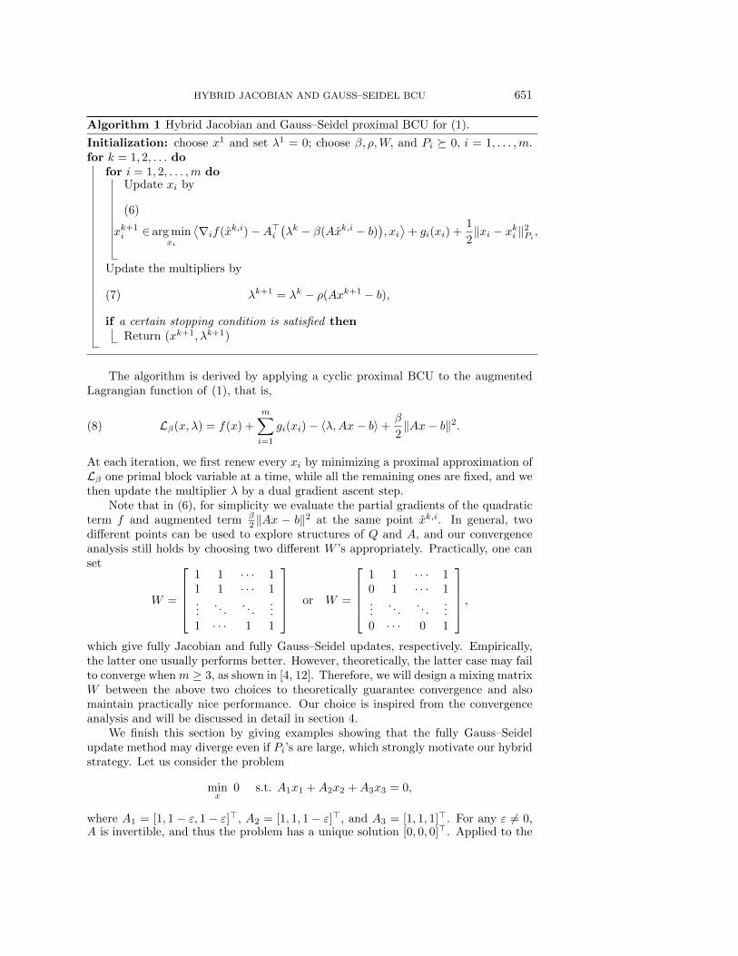
HYBRID JACOBIAN AND GAUSS–SEIDEL BCU 651

Algorithm 1 Hybrid Jacobian and Gauss–Seidel proximal BCU for (1).

Initialization: choose x1 and set λ1 = 0; choose β, ρ,W, and Pi 0, i = 1, . . . ,m.for k = 1, 2, . . . do

for i = 1, 2, . . . ,m doUpdate xi by

xk+1i ∈ arg min

xi

⟨∇if(xk,i)−A>i

(λk − β(Axk,i − b)

), xi⟩

+ gi(xi) +1

2‖xi − xki ‖2Pi

,

(6)

Update the multipliers by

(7) λk+1 = λk − ρ(Axk+1 − b),

if a certain stopping condition is satisfied thenReturn (xk+1, λk+1)

The algorithm is derived by applying a cyclic proximal BCU to the augmentedLagrangian function of (1), that is,

(8) Lβ(x, λ) = f(x) +

m∑i=1

gi(xi)− 〈λ,Ax− b〉+β

2‖Ax− b‖2.

At each iteration, we first renew every xi by minimizing a proximal approximation ofLβ one primal block variable at a time, while all the remaining ones are fixed, and wethen update the multiplier λ by a dual gradient ascent step.

Note that in (6), for simplicity we evaluate the partial gradients of the quadraticterm f and augmented term β

2 ‖Ax − b‖2 at the same point xk,i. In general, twodifferent points can be used to explore structures of Q and A, and our convergenceanalysis still holds by choosing two different W ’s appropriately. Practically, one canset

W =

1 1 · · · 11 1 · · · 1...

. . .. . .

...1 · · · 1 1

or W =

1 1 · · · 10 1 · · · 1...

. . .. . .

...0 · · · 0 1

,which give fully Jacobian and fully Gauss–Seidel updates, respectively. Empirically,the latter one usually performs better. However, theoretically, the latter case may failto converge when m ≥ 3, as shown in [4, 12]. Therefore, we will design a mixing matrixW between the above two choices to theoretically guarantee convergence and alsomaintain practically nice performance. Our choice is inspired from the convergenceanalysis and will be discussed in detail in section 4.

We finish this section by giving examples showing that the fully Gauss–Seidelupdate method may diverge even if Pi’s are large, which strongly motivate our hybridstrategy. Let us consider the problem

minx

0 s.t. A1x1 +A2x2 +A3x3 = 0,

where A1 = [1, 1 − ε, 1 − ε]>, A2 = [1, 1, 1 − ε]>, and A3 = [1, 1, 1]>. For any ε 6= 0,A is invertible, and thus the problem has a unique solution [0, 0, 0]>. Applied to the

652 YANGYANG XU

above problem with fully Gauss–Seidel update, β = ρ = 1, and Pi =maxj ‖Aj‖2

τ ∀i,Algorithm 1 becomes the following iterative method (see [12, section 3]):

xk+11

xk+12

xk+13

λk+1

=

1 0 0 01×3

τA>2 A1 1 0 01×3

τA>3 A1 τA>3 A2 1 01×3

A1 A2 A3 I3×3

−1

×

1− τA>1 A1 −τA>1 A2 −τA>1 A3 τA>1

0 1− τA>2 A2 −τA>2 A3 τA>20 0 1− τA>3 A3 τA>3

03×1 03×1 03×1 I3×3

xk1xk2xk3λk

.Denote Mτ as the iterating matrix. Then the algorithm converges if the spectralradius of Mτ is smaller than one and diverges if larger than one. For ε varyingamong 10−1, 10−2, 10−3, 10−4, we search for the largest τ with initial value 1

3 anddecrement 10−5 such that the spectral radius of Mτ is less than one. The resultsare listed in Table 1 below. They indicate that to guarantee the convergence of thealgorithm, a diminishing stepsize is required for the x-update, but note that τ can beas large as 1

3 for convergence if the fully Jacobian update is employed.

Table 1Values of ε and the corresponding largest τ such that spectral radius of Mτ is less than one.

ε 10−1 10−2 10−3 10−4

τ 1.45473× 10−1 1.34433× 10−2 1.33333× 10−3 1.33333× 10−4

3. Convergence analysis. In this section, we analyze the convergence of Al-gorithm 1. We establish its global iterate sequence convergence and O(1/t) rate bychoosing an appropriate mixing matrix W and assuming merely weak convexity onthe problem.

3.1. Notation and preliminary results. Before proceeding with our analysis,we introduce some notation and a few preliminary lemmas.

We let

g(x) =

m∑i=1

gi(xi), F = f + g.

A point x∗ is a solution to (1) if there exists λ∗ such that the KKT conditions hold:

0 ∈ ∂F (x∗)−A>λ∗,(9a)

Ax∗ − b = 0,(9b)

where ∂F denotes the subdifferential of F . Together with the convexity of F , (9)implies

(10) F (x)− F (x∗)− 〈λ∗, Ax− b〉 ≥ 0 ∀x.

We denote X ∗ as the solution set of (1). For any vector v and any symmetric matrixS of appropriate size, we define ‖v‖2S = v>Sv. Note this definition does not requireS to be PSD, so ‖v‖2S may be negative. I is reserved for the identity matrix and Efor the all-ones matrix, whose size is clear from the context. A ⊗ B represents the

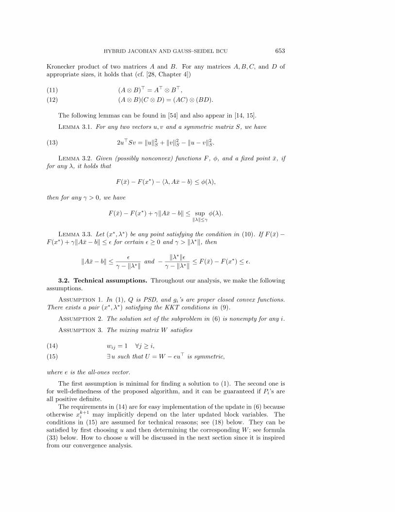
HYBRID JACOBIAN AND GAUSS–SEIDEL BCU 653

Kronecker product of two matrices A and B. For any matrices A,B,C, and D ofappropriate sizes, it holds that (cf. [28, Chapter 4])

(A⊗B)> = A> ⊗B>,(11)

(A⊗B)(C ⊗D) = (AC)⊗ (BD).(12)

The following lemmas can be found in [54] and also appear in [14, 15].

Lemma 3.1. For any two vectors u, v and a symmetric matrix S, we have

(13) 2u>Sv = ‖u‖2S + ‖v‖2S − ‖u− v‖2S .

Lemma 3.2. Given (possibly nonconvex) functions F , φ, and a fixed point x, iffor any λ, it holds that

F (x)− F (x∗)− 〈λ,Ax− b〉 ≤ φ(λ),

then for any γ > 0, we have

F (x)− F (x∗) + γ‖Ax− b‖ ≤ sup‖λ‖≤γ

φ(λ).

Lemma 3.3. Let (x∗, λ∗) be any point satisfying the condition in (10). If F (x)−F (x∗) + γ‖Ax− b‖ ≤ ε for certain ε ≥ 0 and γ > ‖λ∗‖, then

‖Ax− b‖ ≤ ε

γ − ‖λ∗‖and − ‖λ∗‖ε

γ − ‖λ∗‖≤ F (x)− F (x∗) ≤ ε.

3.2. Technical assumptions. Throughout our analysis, we make the followingassumptions.

Assumption 1. In (1), Q is PSD, and gi’s are proper closed convex functions.There exists a pair (x∗, λ∗) satisfying the KKT conditions in (9).

Assumption 2. The solution set of the subproblem in (6) is nonempty for any i.

Assumption 3. The mixing matrix W satisfies

wij = 1 ∀j ≥ i,(14)

∃u such that U = W − eu> is symmetric,(15)

where e is the all-ones vector.

The first assumption is minimal for finding a solution to (1). The second one isfor well-definedness of the proposed algorithm, and it can be guaranteed if Pi’s areall positive definite.

The requirements in (14) are for easy implementation of the update in (6) becauseotherwise xk+1

i may implicitly depend on the later updated block variables. Theconditions in (15) are assumed for technical reasons; see (18) below. They can besatisfied by first choosing u and then determining the corresponding W ; see formula(33) below. How to choose u will be discussed in the next section since it is inspiredfrom our convergence analysis.

654 YANGYANG XU

3.3. Convergence results of Algorithm 1. We show that with appropriateproximal terms, Algorithm 1 can have O(1/t) convergence rate, where t is the numberof iterations. The result includes several existing ones as special cases, and we willdiscuss it after presenting our convergence result.

We first establish a few inequalities. Since Q is PSD, there exists a matrix Hsuch that Q = H>H. Corresponding to the partition of x, we let H = (H1, . . . ,Hm).

Proposition 3.4. Let W satisfy the conditions in Assumption 3 and define

yi = Hixi, zi = Aixi ∀i.

Then for any α > 0,

m∑i=1

m∑j=1

wij⟨Hi(x

k+1i − xi), Hj(x

k+1j − xkj )

⟩(16)

≤ 1

2

(‖yk+1 − y‖2V − ‖yk − y‖2V + ‖yk+1 − yk‖2V

)+

1

2α‖H(xk+1 − x)‖2 +

α

2

∥∥(u> ⊗ I)(yk+1 − yk)∥∥2

and

m∑i=1

m∑j=1

wij⟨Ai(x

k+1i − xi), Aj(xk+1

j − xkj )⟩

(17)

≤ 1

2

(‖zk+1 − z‖2V − ‖zk − z‖2V + ‖zk+1 − zk‖2V

)+

1

2α‖A(xk+1 − b)‖2 +

α

2

∥∥(u> ⊗ I)(zk+1 − zk)∥∥2,

where V = U ⊗ I.

Proof. We only show (16), and (17) follows in the same way. By the definition ofy, we have

m∑i=1

m∑j=1

wij⟨Hi(x

k+1i − xi), Hj(x

k+1j − xkj )

⟩(18)

= (yk+1 − y)>(W ⊗ I

)(yk+1 − yk)

(15)= (yk+1 − y)>

(U ⊗ I

)(yk+1 − yk) + (yk+1 − y)>

((eu>)⊗ I

)(yk+1 − yk)

(12)= (yk+1 − y)>

(U ⊗ I

)(yk+1 − yk) + (yk+1 − y)>

((e⊗ I)

(u> ⊗ I

))(yk+1 − yk)

= (yk+1 − y)>(U ⊗ I

)(yk+1 − yk) +

(H(xk+1 − x)

)> (u> ⊗ I

)(yk+1 − yk)

≤ (yk+1 − y)>(U ⊗ I

)(yk+1 − yk) +

1

2α‖H(xk+1 − x)‖2 +

α

2

∥∥(u> ⊗ I)(yk+1 − yk)∥∥2

(13)=

1

2

(‖yk+1 − y‖2V − ‖yk − y‖2V + ‖yk+1 − yk‖2V

)+

1

2α‖H(xk+1 − x)‖2

+α

2

∥∥(u> ⊗ I)(yk+1 − yk)∥∥2,

where the inequality follows from the Cauchy–Schwarz inequality.

HYBRID JACOBIAN AND GAUSS–SEIDEL BCU 655

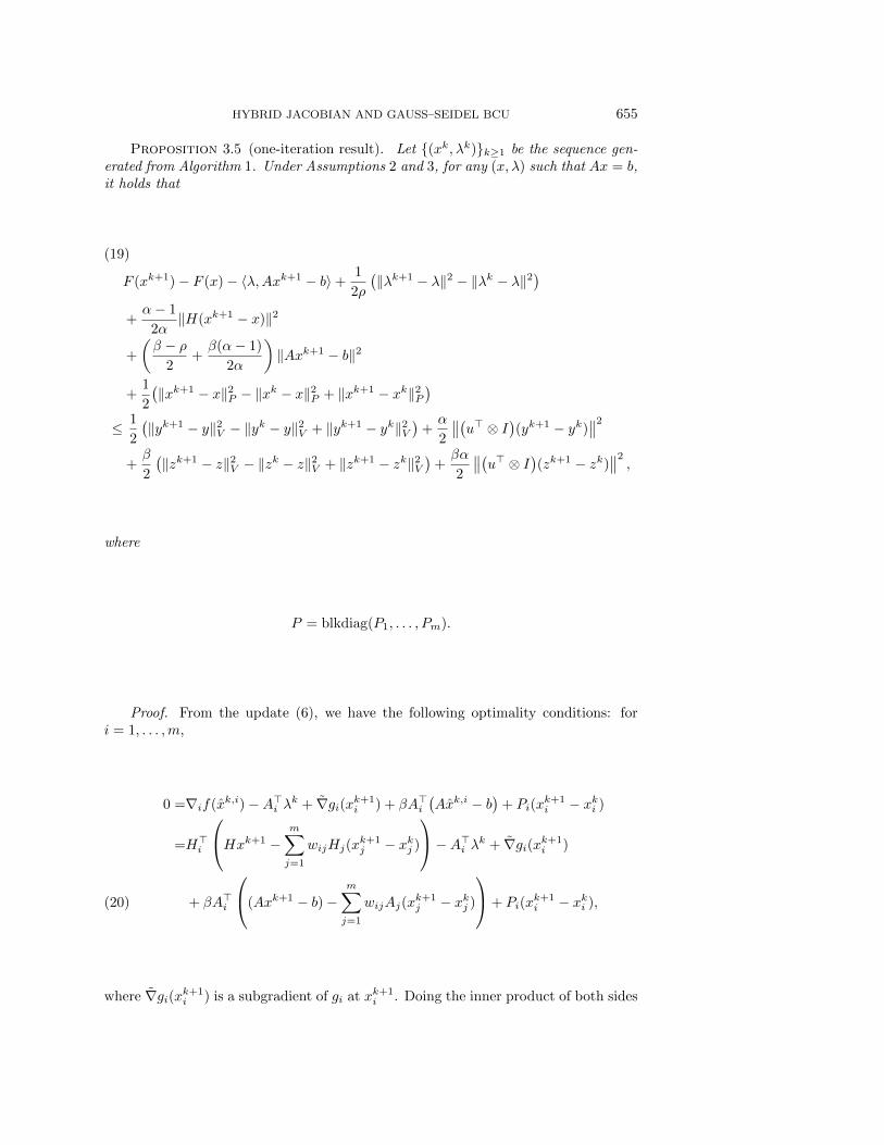
Proposition 3.5 (one-iteration result). Let (xk, λk)k≥1 be the sequence gen-erated from Algorithm 1. Under Assumptions 2 and 3, for any (x, λ) such that Ax = b,it holds that

F (xk+1)− F (x)− 〈λ,Axk+1 − b〉+1

2ρ

(‖λk+1 − λ‖2 − ‖λk − λ‖2

)(19)

+α− 1

2α‖H(xk+1 − x)‖2

+

(β − ρ

2+β(α− 1)

2α

)‖Axk+1 − b‖2

+1

2

(‖xk+1 − x‖2P − ‖xk − x‖2P + ‖xk+1 − xk‖2P

)≤ 1

2

(‖yk+1 − y‖2V − ‖yk − y‖2V + ‖yk+1 − yk‖2V

)+α

2

∥∥(u> ⊗ I)(yk+1 − yk)∥∥2

+β

2

(‖zk+1 − z‖2V − ‖zk − z‖2V + ‖zk+1 − zk‖2V

)+βα

2

∥∥(u> ⊗ I)(zk+1 − zk)∥∥2,

where

P = blkdiag(P1, . . . , Pm).

Proof. From the update (6), we have the following optimality conditions: fori = 1, . . . ,m,

0 =∇if(xk,i)−A>i λk + ∇gi(xk+1i ) + βA>i

(Axk,i − b

)+ Pi(x

k+1i − xki )

=H>i

Hxk+1 −m∑j=1

wijHj(xk+1j − xkj )

−A>i λk + ∇gi(xk+1i )

+ βA>i

(Axk+1 − b)−m∑j=1

wijAj(xk+1j − xkj )

+ Pi(xk+1i − xki ),(20)

where ∇gi(xk+1i ) is a subgradient of gi at xk+1

i . Doing the inner product of both sides

656 YANGYANG XU

of (20) with xk+1i − xi, and summing them together over i, we have

m∑i=1

m∑j=1

wij⟨Hi(x

k+1i − xi), Hj(x

k+1j − xkj )

⟩(21)

+ β

m∑i=1

m∑j=1

wij⟨Ai(x

k+1i − xi), Aj(xk+1

j − xkj )⟩

=⟨H(xk+1 − x), Hxk+1

⟩+⟨A(xk+1 − x),−λk + β(Axk+1 − b)

⟩+⟨xk+1 − x, ∇g(xk+1)

⟩+⟨xk+1 − x, P (xk+1 − xk)

⟩≥⟨H(xk+1 − x), Hxk+1

⟩+⟨A(xk+1 − x),−λk + β(Axk+1 − b)

⟩+ g(xk+1)− g(x)

+⟨xk+1 − x, P (xk+1 − xk)

⟩=

1

2

(‖H(xk+1 − x)‖2 − ‖Hx‖2 + ‖Hxk+1‖2

)− 〈λk+1, Axk+1 − b〉

+ (β − ρ)‖Axk+1 − b‖2 + g(xk+1)− g(x)

+1

2

(‖xk+1 − x‖2P − ‖xk − x‖2P + ‖xk+1 − xk‖2P

)=

1

2‖H(xk+1 − x)‖2 + F (xk+1)− F (x)− 〈λk+1, Axk+1 − b〉

+ (β − ρ)‖Axk+1 − b‖2 +1

2

(‖xk+1 − x‖2P − ‖xk − x‖2P + ‖xk+1 − xk‖2P

),

where the inequality uses the convexity of g, and in the second equality, we have used(13), the update rule (7), and the condition Ax = b.

Substituting (16) and (17) into (21), we have

F (xk+1)− F (x)− 〈λk+1, Axk+1 − b〉+α− 1

2α‖H(xk+1 − x)‖2

(22)

+

(β

2+β(α− 1)

2α− ρ)‖Axk+1 − b‖2

+1

2

(‖xk+1 − x‖2P − ‖xk − x‖2P + ‖xk+1 − xk‖2P

)≤ 1

2

(‖yk+1 − y‖2V − ‖yk − y‖2V + ‖yk+1 − yk‖2V

)+α

2

∥∥(u> ⊗ I)(yk+1 − yk)∥∥2

+β

2

(‖zk+1 − z‖2V − ‖zk − z‖2V + ‖zk+1 − zk‖2V

)+βα

2

∥∥(u> ⊗ I)(zk+1 − zk)∥∥2.

From update (7), we have

0 =〈λk+1 − λ,Axk+1 − b〉+1

ρ〈λk+1 − λ, λk+1 − λk〉

(13)= 〈λk+1 − λ,Axk+1 − b〉+

1

2ρ

(‖λk+1 − λ‖2 − ‖λk − λ‖2 + ‖λk+1 − λk‖2

)= 〈λk+1 − λ,Axk+1 − b〉+

1

2ρ

(‖λk+1 − λ‖2 − ‖λk − λ‖2

)+ρ

2‖Axk+1 − b‖2.(23)

HYBRID JACOBIAN AND GAUSS–SEIDEL BCU 657

Summing (22) and (23) together gives the desired result.Now we are ready to present our main result.

Theorem 3.6. Under Assumptions 1–3, let (xk, λk)k≥1 be the sequence gener-ated from Algorithm 1 with parameters

β ≥ ρ > 0,(24)

P−D>H((W−eu>+αuu>)⊗I

)DH−βD>A

((W−eu>+αuu>)⊗I

)DA := P 0,(25)

where α ≥ 1, and

DH = blkdiag(H1, . . . ,Hm), DA = blkdiag(A1, . . . , Am).

Let xt+1 =∑tk=1

xk+1

t . Then

∣∣F (xt+1)−F (x∗)∣∣≤ 1

2t

(max(1 + ‖λ∗‖)2, 4‖λ∗‖2

ρ+‖x1−x∗‖2P−‖y1−y∗‖2V −β‖z1−z∗‖2V

),

(26a)

‖Axt+1−b‖≤ 1

2t

(max(1 + ‖λ∗‖)2, 4‖λ∗‖2

ρ+‖x1−x∗‖2P−‖y1−y∗‖2V −β‖z1 − z∗‖2V

),

(26b)

where V is defined as in Proposition 3.4, and (x∗, λ∗) is any point satisfying the KKTconditions in (9).

In addition, if α > 1 and P 0, then (xk, λk) converges to a point (x∞, λ∞) thatsatisfies the KKT conditions in (9).

Proof. Summing the inequality (19) from k = 1 through t and noting β ≥ ρ, wehave

t∑k=1

[F (xk+1)− F (x)− 〈λ,Axk+1 − b〉

]+

1

2ρ‖λt+1 − λ‖2 +

1

2‖xt+1 − x‖2P

+

t∑k=1

(1

2‖xk+1 − xk‖2P +

α− 1

2α‖H(xk+1 − x)‖2 +

β(α− 1)

2α‖Axk+1 − b‖2

)≤ 1

2ρ‖λ1 − λ‖2 +

1

2‖x1 − x‖2P −

1

2‖y1 − y‖2V −

β

2‖z1 − z‖2V(27)

+1

2‖yt+1 − y‖2V +

1

2

t∑k=1

‖yk+1 − yk‖2V +α

2

t∑k=1

∥∥(u> ⊗ I)(yk+1 − yk)∥∥2

+β

2‖zt+1 − z‖2V +

β

2

t∑k=1

‖zk+1 − zk‖2V +βα

2

t∑k=1

∥∥(u> ⊗ I)(zk+1 − zk)∥∥2.

Note that

‖yk+1 − yk‖2V + α∥∥(u> ⊗ I)(yk+1 − yk)

∥∥2

= (yk+1 − yk)>(V + αuu> ⊗ I)(yk+1 − yk)

= (xk+1 − xk)>D>H((W − eu> + αuu>)⊗ I

)DH(xk+1 − xk),

and similarly,

‖zk+1 − zk‖2V + α∥∥(u> ⊗ I)(zk+1 − zk)

∥∥2

= (xk+1 − xk)>D>A((W − eu> + αuu>)⊗ I

)DA(xk+1 − xk).

658 YANGYANG XU

Hence, by the choice of P in (25), we have from (27) that

t∑k=1

[F (xk+1)− F (x)− 〈λ,Axk+1 − b〉

]+

1

2ρ‖λt+1 − λ‖2

+

t∑k=1

(1

2‖xk+1 − xk‖2

P+α− 1

2α‖H(xk+1 − x)‖2 +

β(α− 1)

2α‖Axk+1 − b‖2

)≤ 1

2ρ‖λ1 − λ‖2 +

1

2‖x1 − x‖2P −

1

2‖y1 − y‖2V −

β

2‖z1 − z‖2V .(28)

Since α ≥ 1 and P 0, it follows from the above inequality and the convexity ofF that

F (xt+1)− F (x∗)− 〈λ,Axt+1 − b〉(29)

≤ 1

2t

(1

ρ‖λ1 − λ‖2 + ‖x1 − x∗‖2P − ‖y1 − y∗‖2V − β‖z1 − z∗‖2V

).

Since λ1 = 0, we use Lemmas 3.2 and 3.3 with γ = max1 + ‖λ∗‖, 2‖λ∗‖ to obtain(26).

If α > 1 and P 0, then letting x = x∗, λ = λ∗ in (28) and also using (10), wehave

(30) limk→∞

(xk+1 − xk) = 0, limk→∞

(λk+1 − λk) = −ρ limk→∞

(Axk+1 − b) = 0,

and thus

(31) limk→∞

(xk − xk,i) = 0 ∀i.

On the other hand, letting (x, λ) = (x∗, λ∗) in (19), using (10), and noting α, α ≥ 1,we have

1

2ρ‖λk+1 − λ∗‖2 +

1

2

(‖xk+1 − x∗‖2P − ‖yk+1 − y∗‖2V − β‖zk+1 − z∗‖2V

)≤ 1

2ρ‖λk − λ∗‖2 +

1

2

(‖xk − x∗‖2P − ‖yk − y∗‖2V − β‖zk − z∗‖2V

),(32)

which, together with the choice of P, indicates the boundedness of (xk, λk)k≥1.Hence, it must have a finite cluster point (x∞, λ∞), and there is a subsequence(xk, λk)k∈K convergent to this cluster point. From (30), it immediately followsthat Ax∞ − b = 0. In addition, letting K 3 k → ∞ in (6) and using (30) and (31)gives

x∞i = arg minxi

〈∇if(x∞)−A>i λ∞, xi〉+ gi(xi) +1

2‖xi − x∞i ‖2Pi

∀i,

and thus the following optimality condition holds:

0 ∈ ∇if(x∞) + ∂gi(x∞i )−A>i λ∞ ∀i.

Therefore, (x∞, λ∞) satisfies the conditions in (9). Since (32) holds for any point(x∗, λ∗) satisfying (9), it also holds with (x∗, λ∗) = (x∞, λ∞). Denote

v = (x, λ), S =

[P −D>HV DH − βD>AV DA 0

0 Iρ

].

HYBRID JACOBIAN AND GAUSS–SEIDEL BCU 659

Then letting (x∗, λ∗) = (x∞, λ∞) in (32), we have ‖vk+1−v∞‖S ≤ ‖vk−v∞‖S . From(25) and P 0, it follows that S 0, and hence vk gets closer to v∞ as k increases.Because (x∞, λ∞) is a cluster point of (xk, λk)k≥1, we obtain the convergence of(xk, λk) to (x∞, λ∞) and complete the proof.

4. How to choose a mixing matrix. In this section, we discuss how to chooseW such that it satisfies Assumption 3. Note that the upper triangular part of Whas been fixed, and we need only set its strictly lower triangular part. Denote U(W )and L(W ), respectively, as the upper and strictly lower triangular parts of W , i.e.,W = L(W ) + U(W ), and thus (15) is equivalent to requiring the existence of u suchthat

L(W ) + U(W )− eu> = L(W )> + U(W )> − ue>.

It suffices to let

(33) L(W ) = L(W> + eu> − ue>) = L(eu> − ue> + E).

Therefore, given any vector u, we can find a corresponding W by setting its uppertriangular part to all ones and its strictly lower triangular part according to the aboveformula.

4.1. Finding u by solving an SDP. Theoretically, proximal terms help con-vergence guarantee of the algorithm. However, empirically, these terms can slow theconvergence speed. Based on these observations, we aim at finding a block diagonalP such that (25) holds and also is as close to zero as possible.

One choice of P satisfying (25) could be

(34) Pi = (1−Di)H>i Hi + β(1−Di)A

>i Ai + d(‖Hi‖22 + β‖Ai‖22)I, i = 1, . . . ,m,

where D = diag(D1, . . . , Dm) with each Di ∈ 0, 1 for each i, and

(35) dI (1 + β)(W − eu> + αuu>)− (1 + β)(I −D).

Note that if Pi = ηiI +H>i Hi, then (6) reduces to

(36) xk+1i ∈ arg min

xi

f(xi, xk,i6=i)−

⟨A>i(λk − β(Axk,i − b)

), xi⟩+gi(xi)+

ηi2‖xi−xki ‖2.

Hence, Di = 0 indicates no linearization to f or ‖Ax−b‖2 at xki , and Di = 1 indicateslinearization to them. If (36) is easy to solve, one can set Di = 0. Otherwise, Di = 1is recommended to have easier subproblems.

With D fixed, to obtain P according to (34), we need only specify the value ofd. Recall that we aim at finding a close-to-zero P , so it would be desirable to chooseu such that d is as small as possible. For simplicity, we set α = 1. Therefore, tominimize d, we solve the following optimization problem:

(37) minu,W

λmax

(W − eu> + uu> − I +D

)s.t. W − eu> = W> − ue>,

where λmax(B) denotes the maximum eigenvalue of a symmetric matrix B.Using (33), we represent W by u and write (37) equivalently to

(38) minuλmax

(L(eu> − ue>) + E − eu> + uu> − I +D

),

660 YANGYANG XU

which can be further formulated as an SDP by the relation between the positive-definiteness of a 2 × 2 block matrix and its Schur complement (cf. [1, AppendixA.5.5]):

(39)

[A BB> C

] 0⇔ A−BC−1B> 0,

where A is symmetric and C 0. Let

σ = λmax

(L(eu> − ue>) + E − eu> + uu> − I +D

).

ThenσI L(eu> − ue>) + E − eu> + uu> − I +D,

and by (39) it is equivalent to[(σ + 1)I −D − L(eu> − ue>)− E + eu> u

u> 1

] 0.

Therefore, (38) is equivalent to the SDP

(40) minσ,u

σ s.t.

[(σ + 1)I −D − L(eu> − ue>)− E + eu> u

u> 1

] 0.

Note that problem (1) can be extremely large. However, the dimension (i.e., m) ofthe SDP (40) could be much smaller (see examples in section 5) and can be efficientlyand accurately solved by the interior-point method. In addition, (40) does not dependon the data matrix H and A, so we can solve it offline.

If the sizes of H and A are not large, upon solving (40), one can explicitly form thematrix D>H

((W − eu>+uu>)⊗ I

)DH +βD>A

((W − eu>+uu>)⊗ I

)DA and compute

its spectral norm. This way, one can have a smaller P . However, for large-scale H orA, it can be overwhelmingly expensive to do so.

In addition, note that we can add more constraints to (40) to obtain a desiredW . For instance, we can partition the m blocks into several groups. Then we updatethe blocks in the same group in parallel in Jacobian manner and cyclically renew thegroups. This corresponds to fixing a few block matrices in the lower triangular partof W to all ones.

4.2. Special cases. A few special cases are as follows.• If u is the zero vector, then by (33), we have the lower triangular part ofW to be all ones, and this way gives a fully Jacobian BCU method. Hence,Theorem 3.6 applies for the Jacobian update method. In this case, if D = Iin (35), then we have d ≥ (1 + β)m that is significantly greater than theoptimal value of (40).

• If we enforce the lower triangular part of W to all zeros, Algorithm 1 will re-duce to a fully Gauss–Seidel BCU method. However, adding such constraintsinto (40) would lead to infeasibility. Hence, Theorem 3.6 does not apply tothis case.

• If m = 2 and D = 0, i.e., if there were only two blocks and no linearization isperformed, solving (40) would give the solution σ = 0 and u = (0, 1)>. Thisway, we have

W =

[1 10 1

], P =

[H>1 H1 + βA>1 A1 0

0 H>2 H2 + βA>2 A2

]

HYBRID JACOBIAN AND GAUSS–SEIDEL BCU 661

and thus recover the two-block ADMM with nonseparable quadratic termf in the objective. Theorem 3.6 implies an O(1/t) convergence rate for thiscase, and it improves the result in [5], which shows convergence of this specialcase but without rate estimate.

4.3. Different mixing matrices. We can choose two different W ’s to explorethe structures of A and Q. Let us give an example to illustrate this. Suppose A is ageneric matrix and Q block tridiagonal. The W used to linearize the augmented termβ2 ‖Ax − b‖

2 can be set in the way discussed in section 4.1. For the mixing matrixto Q, we note H>i Hj = 0 if |i − j| > 1. Then the left-hand side of (16) becomes∑|i−j|≤1 wij

⟨Hi(x

k+1i −xi), Hj(x

k+1j −xkj )

⟩. Hence, following our analysis, we would

require that there exist u such that W −e>u is symmetric, where wij = 0 if |i−j| > 1

and wij = 1 if i ≤ j ≤ i+ 1. To completely determine W , we need only set its valueson the subdiagonal. Similarly to (37), we can find u and wi+1,i’s through solving

minu,W

λmax

(W − eu> + uu> − I +D

)s.t. W − eu> = W> − ue>, wij = 0 ∀|i− j| > 1, wij = 1, i ≤ j ≤ i+ 1.

The optimal value of the above problem is significantly smaller than that of (37), andthus in (34) the coefficient before ‖Hi‖2 can be set smaller. This way, we will havesmaller Pi’s, which potentially can make the algorithm converge faster.

5. Numerical experiments. In this section, we apply Algorithm 1 to threeproblems: quadratic programming, compressive principal component pursuit, and theMSVM problem. We test it with two different mixing matrices: the all-ones matrixand the matrix given by the method discussed in section 4.1. The former correspondsto a fully Jacobian update method and the latter to a hybrid Jacobian and Gauss–Seidel method, dubbed Jacobi-PC and JaGS-PC, respectively. We compare them to arecently proposed randomized proximal BCU method (named random-PC) in [15], theADMM with Gauss back substitution (named as ADMM-GBS) in [21], and also thedirect ADMM. Note that the direct ADMM is not guaranteed to converge for problemswith more than two blocks, but empirically it can often perform well. ADMM-GBS isdesigned for separable multiblock convex problems. It does not allow linearization tothe augmented term. In addition, it requires all Ai’s to be full-column rank. Hence,the proposed algorithm is applicable to a broader class of problems, but we observethat JaGS-PC can be comparable to direct ADMM and ADMM-GBS.

We choose to compare with random-PC, direct ADMM, and ADMM-GBS be-cause, as well as the proposed methods, all of them have low per-iteration complexityand low memory requirement and belong to the inexact ALM framework. On solvingthe three problems, one can also apply some other methods, such as the interior-point method and the projected subgradient method. The interior-point method canconverge faster than the proposed ones in terms of iteration number. However, itsper-iteration complexity is much higher, and thus total running time can be longer(that is observed for quadratic programming). In addition, it has a high demandon machine memory and may be inapplicable for large-scale problems, such as thecompressive principal component pursuit. The projected subgradient method hasper-iteration complexity similar to the proposed ones but converges much slower.

In all our tests, we report the results based on the actual iterate xk, which isguaranteed to converge to an optimal solution. Although the convergence rate inTheorem 3.6 is based on the averaged point xt+1 (i.e., in ergodic sense), numerically

662 YANGYANG XU

we notice that the convergence speed based on the iterate xk is often faster than thatbased on the averaged point. This phenomenon also happens to the classic two-blockADMM. The work [24] shows that ADMM has an ergodic sublinear convergence rate,but all applications of ADMM still use the actual iterate as the solution.

5.1. Adaptive proximal terms. As we mentioned previously, the proximalterms used in (6) help the convergence guarantee but can empirically slow the conver-gence speed (see Figures 1 and 2). Here, we set Pi’s similarly to (34) but in a simpleadaptive way as follows:

(41) P ki = (1−Di)H>i Hi + β(1−Di)A

>i Ai + dk(‖Hi‖22 + β‖Ai‖22)I, i = 1, . . . ,m.

After each iteration k, we check whether the following inequality holds:

η‖xk+1 − xk‖2Pk ≤ ‖yk+1 − yk‖2V +∥∥(u> ⊗ I)(yk+1 − yk)

∥∥2(42)

+ β‖zk+1 − zk‖2V + β∥∥(u> ⊗ I)(zk+1 − zk)

∥∥2,

and set

(43) dk =

min

(dk−1 + dinc, dmax

)if (42) holds,

dk−1 otherwise,

where dinc is a small positive number, and η = 0.999 is used1 in all the tests. Forstability and also efficiency, we choose d1 and dinc such that (42) does not happenmany times. Specifically, we first run the algorithm to 20 iterations with (d1, dinc)selected from 0, 0.5, 1×0.01, 0.1. If there is one pair of values such that (42) doesnot always hold within the 20 iterations,2 we accept that pair of (d1, dinc). Otherwise,we simply set dk = dmax ∀k. For Jacobi-PC, we set dmax = λmax(E − I +D), and forJaGS-PC, we set dmax to the optimal value of (40), which is solved by SDPT3 [46]to high accuracy with stopping tolerance 10−12. Note that as long as dinc is positive,dk can only be incremented finitely many times, and thus (42) can only happen infinitely many iterations. In addition, note that both sides of (42) can be evaluated ascheaply as computing x>Qx and x>A>Ax.

The above adaptive way of setting P k is inspired by our convergence analysis. If,after k0 iterations, (42) never holds, then we can also show a sublinear convergenceresult by summing (19) from k = k0 through t and then following the same argumentsas those in the proof of Theorem 3.6.

5.2. Quadratic programming. We test Jacobi-PC and JaGS-PC on the non-negative linearly constrained quadratic programming

(44) minxF (x) =

1

2x>Qx+ c>x s.t. Ax = b, x ≥ 0,

where Q ∈ Rn×n is a symmetric PSD matrix, A ∈ Rp×n, and b ∈ Rp, c ∈ Rn. Inthe test, we set p = 200, n = 2000, and Q = H>H with H ∈ R(n−10)×n generated

1In the proof of Theorem 3.6, we bound the y- and z-terms by the x-term. If the left-handside of (42) with η < 1 can upper bound the right-hand side, then Theorem 3.6 guarantees theconvergence of xk to an optimal solution. Numerically, taking η close to 1 would make the algorithmmore efficient.

2We notice that if (42) happens many times, the iterate may be far away from the optimalsolution in the beginning, and that may affect the overall performance; see Figures 3 and 5.

HYBRID JACOBIAN AND GAUSS–SEIDEL BCU 663

0 100 200 300 400 500

Epoch numbers

100

102

104

106

Dis

tanc

e of

obj

ectiv

e to

opt

imal

val

ue

nonadaptive JaGS-PCnonadaptive Jacobi-PC

0 100 200 300 400 500

Epoch numbers

10-2

10-1

100

101

102

103

Vio

latio

n of

feas

ibili

ty

nonadaptive JaGS-PCnonadaptive Jacobi-PC

Fig. 1. Results by applying Jacobi-PC and JaGS-PC without adapting proximal terms on thequadratic programming (44). Left: the distance of the objective to optimal value |F (xk) − F (x∗)|.Right: the violation of feasibility ‖Axk − b‖.

according to the standard Gaussian distribution. This generated Q is degenerate,and thus the problem is only weakly convex. The entries of c follow i.i.d. standardGaussian distribution, and those of b follow from uniform distribution on [0, 1]. Weset A = [B, I] to guarantee feasibility of the problem, with B generated according tostandard Gaussian distribution.

We evenly partition the variable x into m = 40 blocks, each one consisting of 50coordinates. The same values of parameters are set for both Jacobi-PC and JaGS-PCas follows:

β = ρ = 1, D = I, d1 = 0.5, dinc = 0.1.

They are compared to random-PC that uses the same penalty parameter β = 1 andρ = 1

m according to the analysis in [15]. We also adaptively increase the proximalparameter of random-PC in a way similar to that in section 5.1. All three methods runto 500 epochs, where each epoch is equivalent to updating all blocks one time. Theirper-epoch complexity is almost the same. To evaluate their performance, we computethe distance of the objective to optimal value |F (xk) − F (x∗)| and the violation offeasibility ‖Axk − b‖ at each iteration k, where the optimal solution is obtained byMATLAB solver quadprog with the “interior-point-convex” option. Figures 1 and 2plot the results by the three methods in terms of both iteration number and runningtime (sec). In Figure 1, we simply set dk = dmax for Jacobi-PC and JaGS-PC, i.e.,without adapting the proximal terms, where in this test, dmax = 18.3273 for JaGS-PCand dmax = 40 for Jacobi-PC. From the figures, we see that JaGS-PC is significantlyfaster than Jacobi-PC in terms of both objective and feasibility for both adaptive andnonadaptive cases, and random-PC is slightly slower than JaGS-PC.

5.3. Compressive principal component pursuit. In this subsection, we testJacobi-PC and JaGS-PC on

(45) minX,Y

F (X,Y ) = µ‖X‖1 + ‖Y ‖∗ s.t. A(X + Y ) = b,

where ‖X‖1 =∑i,j |Xij |, ‖Y ‖∗ denotes the matrix operator norm and equals the

largest singular value of Y , A is a linear operator, and b contains the measurements.If A is the identity operator, (45) is called the principal component pursuit proposedin [3], and it is called compressive PCP [52] when A is an underdetermined measuringoperator. We consider the sampling operator, i.e., A = PΩ, where Ω is an index setand PΩ is a projection keeping the entries in Ω and zeroing out all others.

Assume M to be the underlying matrix and b = A(M). Upon solving (45),X + Y recovers M with sparse part X and low-rank part Y . We use the Escalator

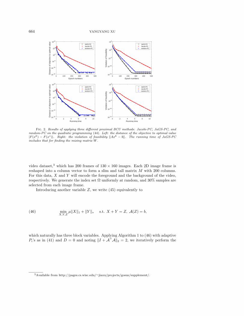
664 YANGYANG XU

0 100 200 300 400 500

Epoch numbers

10-15

10-10

10-5

100

105

1010

Dis

tanc

e of

obj

ectiv

e to

opt

imal

val

ue

JaGS-PCJacobi-PCrandom-PC

0 100 200 300 400 500

Epoch numbers

10-15

10-10

10-5

100

105

Vio

latio

n of

feas

ibili

ty

JaGS-PCJacobi-PCrandom-PC

0 2 4 6 8 10

Running time

10-15

10-10

10-5

100

105

1010

Dis

tanc

e of

obj

ectiv

e to

opt

imal

val

ue

JaGS-PCJacobi-PCrandom-PC

0 2 4 6 8 10

Running time

10-15

10-10

10-5

100

105

Vio

latio

n of

feas

ibili

ty

JaGS-PCJacobi-PCrandom-PC

Fig. 2. Results of applying three different proximal BCU methods: Jacobi-PC, JaGS-PC, andrandom-PC on the quadratic programming (44). Left: the distance of the objective to optimal value|F (xk) − F (x∗)|. Right: the violation of feasibility ‖Axk − b‖. The running time of JaGS-PCincludes that for finding the mixing matrix W .

video dataset,3 which has 200 frames of 130 × 160 images. Each 2D image frame isreshaped into a column vector to form a slim and tall matrix M with 200 columns.For this data, X and Y will encode the foreground and the background of the video,respectively. We generate the index set Ω uniformly at random, and 30% samples areselected from each image frame.

Introducing another variable Z, we write (45) equivalently to

(46) minX,Y,Z

µ‖X‖1 + ‖Y ‖∗ s.t. X + Y = Z, A(Z) = b,

which naturally has three block variables. Applying Algorithm 1 to (46) with adaptivePi’s as in (41) and D = 0 and noting ‖I + A>A‖2 = 2, we iteratively perform the

3Available from http://pages.cs.wisc.edu/∼jiaxu/projects/gosus/supplement/.

HYBRID JACOBIAN AND GAUSS–SEIDEL BCU 665

updates:

Xk+1 = arg minX

µ‖X‖1 − 〈Λk, X〉+β

2‖X + Y k − Zk‖2F +

dkβ

2‖X −Xk‖2,

(47a)

Y k+1 = arg minY

‖Y ‖∗ − 〈Λk, Y 〉+β

2‖Xk + Y − Zk‖2F +

dkβ

2‖Y − Y k‖2,

(47b)

Zk+1 =arg minZ〈Λk−A>(Πk), Z〉+ β

2‖Xk+Y k−Zk‖2F +

β

2‖A(Z)−b‖2+dkβ‖Z−Zk‖2,

(47c)

Λk+1 = Λk − ρ(Xk+1 + Y k+1 − Zk+1),

(47d)

Πk+1 = Πk − ρ(A(Zk+1)− b).(47e)

Since AA> = I, all three primal subproblems have closed-form solutions. We setβ = ρ = 0.05 and dinc = 0.01 for both JaGS-PC and Jacobi-PC methods, and setd1 = 0 for JaGS-PC and d1 = 1 for Jacobi-PC because the latter can deviate fromoptimality very far away in the beginning if it starts with a small d1 (see Figure3). They are compared to random-PC, direct ADMM, and ADMM-GBS. At everyiteration, random-PC performs one update among (47a)—(47c) with dk = 0 and thenupdates Λ and Π by (47d) and (47e) with ρ = β

3 ; the direct ADMM sets dk = 0∀k in(47); and ADMM-GBS runs the direct ADMM first and then performs a correctionstep by Gauss back substitution. We use the same β and ρ for the direct ADMMand ADMM-GBS and set the correction step parameter of ADMM-GBS to 0.99.On solving the SDP (40), we have for JaGS-PC dmax = 0.4270 and the mixing matrix,

W =

1 1 10.3691 1 1−0.2618 0.3691 1

.Figure 4 plots the results by all five methods, where the optimal solution is obtained byrunning JaGS-PC to 10,000 epochs. From the figure, we see that JaGS-PC performssignificantly better than Jacobi-PC. and JaGS-PC; direct ADMM and ADMM-GBSperform almost the same; and random-PC performs the worst. Note that althoughdirect ADMM works well on this example, its convergence is not guaranteed in general.

5.4. Multiclass support vector machine. In this subsection, we test Jacobi-PC, JaGS-PC, and random-PC on the MSVM problem that is considered in [55]:

(48) minX

F (X) =1

n

n∑i=1

c∑j=1

ι·6=j(bi)[x>j ai + 1]+ + µ‖X‖1 s.t. Xe = 0,

where xj is the jth column of X, (ai, bi)ni=1 is the training dataset with label bi ∈1, . . . , c ∀i, ι·6=j(bi) equals one if bi 6= j and zero otherwise, and [d]+ = max(0, d).We set the number of classes to c = 3 and randomly generate the data according toGaussian distribution N (vj ,Σj) for the jth class, where vj ∈ Rp and Σj ∈ Rp×p for

666 YANGYANG XU

0 100 200 300 400 500

Iteration numbers

100

1010

1020

1030

1040

Dis

tanc

e of

obj

ectiv

e to

opt

imal

val

ue

Jacobi-PC

0 100 200 300 400 500

Iteration numbers

1010

1020

1030

1040

Vio

latio

n of

feas

ibili

ty

Jacobi-PC

Fig. 3. Results of Jacobi-PC with d1 = 0 and dinc = 0.01 for solving the compressive PCP(46) on the Escalator dataset. Left: the relative error between the objective and optimal value|F (Xk,Y k)−F (X∗,Y ∗)|

F (X∗,Y ∗) . Right: relative violation of feasibility:‖Xk+Y k−Zk‖F+‖A(Zk)−b‖F

‖M‖F.

0 100 200 300 400 500

Iteration numbers

10-6

10-4

10-2

100

102

Dis

tanc

e of

obj

ectiv

e to

opt

imal

val

ue

direct ADMMJaGS-PCJacobi-PCADMM-GBSrandom-PC

0 100 200 300 400 500

Iteration numbers

10-4

10-3

10-2

10-1

100

101V

iola

tion

of fe

asib

ility

direct ADMMJaGS-PCJacobi-PCADMM-GBSrandom-PC

0 20 40 60 80 100

Running time

10-6

10-4

10-2

100

102

Dis

tanc

e of

obj

ectiv

e to

opt

imal

val

ue

direct ADMMJaGS-PCJacobi-PCADMM-GBSrandom-PC

0 20 40 60 80 100

Running time

10-4

10-3

10-2

10-1

100

101

Vio

latio

n of

feas

ibili

ty

direct ADMMJaGS-PCJacobi-PCADMM-GBSrandom-PC

Fig. 4. Results by five different methods for solving the compressive PCP (46) on the Escalator

dataset. Left: the relative error between the objective and optimal value|F (Xk,Y k)−F (X∗,Y ∗)|

F (X∗,Y ∗) .

Right: relative violation of feasibility:‖Xk+Y k−Zk‖F+‖A(Zk)−b‖F

‖M‖F. The running time of JaGS-PC

includes that for finding the mixing matrix W .

j = 1, 2, 3 are

v1 =

[Es×1

0

], v2 =

0s/2×1

Es×1

0

, v3 =

0s×1

Es×1

0

, Σ1 =

[σEs×s + (1− σ)I 0

0 I

],

Σ2 =

I s2×

s2

0 00 σEs×s + (1− σ)I 00 0 I

, Σ3 =

Is×s 0 00 σEs×s + (1− σ)I 00 0 I

,where E, I, 0, respectively, represent all-ones, identity, and all-zero matrices of appro-priate sizes, and the subscript specifies the size. The parameter σ measures correlationof features. This kind of dataset has also been used in [56] for testing binary SVM. In

HYBRID JACOBIAN AND GAUSS–SEIDEL BCU 667

0 100 200 300 400 500

Iteration numbers

10-4

10-2

100

102

104

106

Dis

tanc

e of

obj

ectiv

e to

opt

imal

val

ue

Jacobi-PC

0 100 200 300 400 500

Iteration numbers

10-4

10-2

100

102

104

106

Vio

latio

n of

feas

ibili

ty

Jacobi-PC

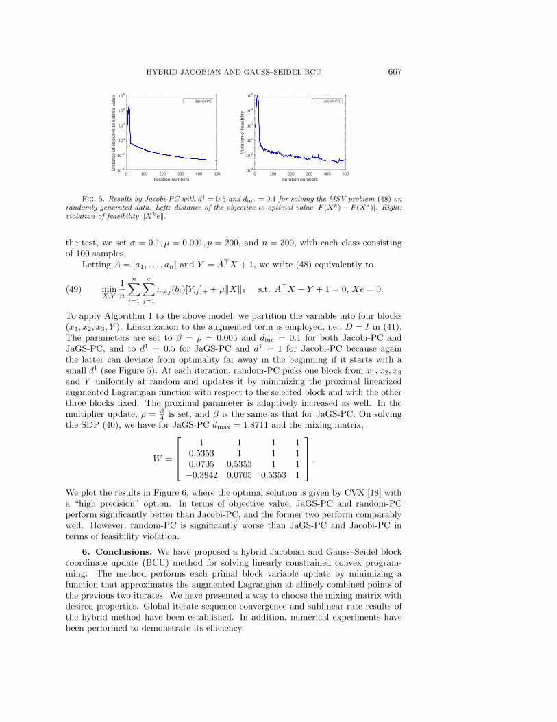
Fig. 5. Results by Jacobi-PC with d1 = 0.5 and dinc = 0.1 for solving the MSV problem (48) onrandomly generated data. Left: distance of the objective to optimal value |F (Xk)− F (X∗)|. Right:violation of feasibility ‖Xke‖.

the test, we set σ = 0.1, µ = 0.001, p = 200, and n = 300, with each class consistingof 100 samples.

Letting A = [a1, . . . , an] and Y = A>X + 1, we write (48) equivalently to

(49) minX,Y

1

n

n∑i=1

c∑j=1

ι·6=j(bi)[Yij ]+ + µ‖X‖1 s.t. A>X − Y + 1 = 0, Xe = 0.

To apply Algorithm 1 to the above model, we partition the variable into four blocks(x1, x2, x3, Y ). Linearization to the augmented term is employed, i.e., D = I in (41).The parameters are set to β = ρ = 0.005 and dinc = 0.1 for both Jacobi-PC andJaGS-PC, and to d1 = 0.5 for JaGS-PC and d1 = 1 for Jacobi-PC because againthe latter can deviate from optimality far away in the beginning if it starts with asmall d1 (see Figure 5). At each iteration, random-PC picks one block from x1, x2, x3

and Y uniformly at random and updates it by minimizing the proximal linearizedaugmented Lagrangian function with respect to the selected block and with the otherthree blocks fixed. The proximal parameter is adaptively increased as well. In themultiplier update, ρ = β

4 is set, and β is the same as that for JaGS-PC. On solvingthe SDP (40), we have for JaGS-PC dmax = 1.8711 and the mixing matrix,

W =

1 1 1 1

0.5353 1 1 10.0705 0.5353 1 1−0.3942 0.0705 0.5353 1

.We plot the results in Figure 6, where the optimal solution is given by CVX [18] witha “high precision” option. In terms of objective value, JaGS-PC and random-PCperform significantly better than Jacobi-PC, and the former two perform comparablywell. However, random-PC is significantly worse than JaGS-PC and Jacobi-PC interms of feasibility violation.

6. Conclusions. We have proposed a hybrid Jacobian and Gauss–Seidel blockcoordinate update (BCU) method for solving linearly constrained convex program-ming. The method performs each primal block variable update by minimizing afunction that approximates the augmented Lagrangian at affinely combined points ofthe previous two iterates. We have presented a way to choose the mixing matrix withdesired properties. Global iterate sequence convergence and sublinear rate results ofthe hybrid method have been established. In addition, numerical experiments havebeen performed to demonstrate its efficiency.

668 YANGYANG XU

0 100 200 300 400 500

Iteration numbers

10-4

10-2

100

102

Dis

tanc

e of

obj

ectiv

e to

opt

imal

val

ue

JaGS-PCJacobi-PCrandom-PC

0 100 200 300 400 500

Iteration numbers

10-4

10-2

100

102

104

Vio

latio

n of

feas

ibili

ty

JaGS-PCJacobi-PCrandom-PC

0 0.05 0.1 0.15 0.2

Running time

10-4

10-2

100

102

Dis

tanc

e of

obj

ectiv

e to

opt

imal

val

ue

JaGS-PCJacobi-PCrandom-PC

0 0.05 0.1 0.15 0.2

Running time

10-4

10-2

100

102

104

Vio

latio

n of

feas

ibili

ty

JaGS-PCJacobi-PCrandom-PC

Fig. 6. Results of Jacobi-PC and JaGS-PC for solving the MSVM problem (48) on randomlygenerated data. Left: distance of the objective to optimal value |F (Xk)− F (X∗)|. Right: violationof feasibility ‖Xke‖. The running time of JaGS-PC includes that for finding the mixing matrix W .

Acknowledgment. The author would like to thank the two anonymous refereesfor their careful review and constructive comments, which helped to greatly improvethe paper.

REFERENCES

[1] S. Boyd and L. Vandenberghe, Convex Optimization, Cambridge University Press, 2004.[2] X. Cai, D. Han, and X. Yuan, The Direct Extension of ADMM for Three-Block Separable

Convex Minimization Models Is Convergent When One Function is Strongly Convex, e-print, Optimization Online, 2014.

[3] E. J. Candes, X. Li, Y. Ma, and J. Wright, Robust principal component analysis?, J. ACM,58 (2011), 11.

[4] C. Chen, B. He, Y. Ye, and X. Yuan, The direct extension of ADMM for multi-block convexminimization problems is not necessarily convergent, Math. Programming, 155 (2016), pp.57–79.

[5] C. Chen, M. Li, X. Liu, and Y. Ye, Extended ADMM and BCD for Nonseparable ConvexMinimization Models with Quadratic Coupling Terms: Convergence Analysis and Insights,preprint, https://arxiv.org/abs/1508.00193, 2015.

[6] C. Chen, Y. Shen, and Y. You, On the convergence analysis of the alternating directionmethod of multipliers with three blocks, Abstract Appl. Anal., 2013, 183961.

[7] P. L. Combettes and J.-C. Pesquet, Stochastic quasi-Fejer block-coordinate fixed pointiterations with random sweeping, SIAM J. Optim., 25 (2015), pp. 1221–1248, https://doi.org/10.1137/140971233.

[8] Y. Cui, X. Li, D. Sun, and K.-C. Toh, On the Convergence Properties of a Majorized ADMMfor Linearly Constrained Convex Optimization Problems with Coupled Objective Func-tions, preprint, https://arxiv.org/abs/1502.00098, 2015.

[9] C. Dang and G. Lan, Randomized Methods for Saddle Point Computation, preprint, https://arxiv.org/abs/1409.8625, 2014.

[10] D. Davis and W. Yin, A Three-Operator Splitting Scheme and Its Optimization Applications,preprint, https://arxiv.org/abs/1504.01032, 2015.

[11] W. Deng, M.-J. Lai, Z. Peng, and W. Yin, Parallel multi-block ADMM with o(1/k) conver-gence, J. Sci. Comput., 71 (2017), pp. 712–736.

HYBRID JACOBIAN AND GAUSS–SEIDEL BCU 669

[12] J.-K. Feng, H.-B. Zhang, C.-Z. Cheng, and H.-M. Pei, Convergence analysis of l-ADMMfor multi-block linear-constrained separable convex minimization problem, J. Oper. Res.Soc. China, 3 (2015), pp. 563–579.

[13] D. Gabay and B. Mercier, A dual algorithm for the solution of nonlinear variational problemsvia finite element approximation, Comput. Math. Appl., 2 (1976), pp. 17–40.

[14] X. Gao, B. Jiang, and S. Zhang, On the Information-Adaptive Variants of the ADMM: AnIteration Complexity Perspective, e-print, Optimization Online, 2014.

[15] X. Gao, Y. Xu, and S. Zhang, Randomized Primal-Dual Proximal Block Coordinate Updates,preprint, https://arxiv.org/abs/1605.05969, 2016.

[16] X. Gao and S.-Z. Zhang, First-order algorithms for convex optimization with nonseparableobjective and coupled constraints, J. Oper. Res. Soc. China, 5 (2017), pp. 131–159.

[17] R. Glowinski and A. Marrocco, Sur l’approximation, par elements finis d’ordre un, et laresolution, par penalisation-dualite d’une classe de problemes de dirichlet non lineaires,ESAIM Math. Model. Numer. Anal., 9 (1975), pp. 41–76.

[18] M. Grant, S. Boyd, and Y. Ye, CVX: MATLAB Software for Disciplined Convex Program-ming, Version 2.1, 2017, http://cvxr.com/cvx/ (accessed 2-5-18).

[19] D. Han and X. Yuan, A note on the alternating direction method of multipliers, J. Optim.Theory Appl., 155 (2012), pp. 227–238.

[20] B. He, L. Hou, and X. Yuan, On full Jacobian decomposition of the augmented Lagrangianmethod for separable convex programming, SIAM J. Optim., 25 (2015), pp. 2274–2312,https://doi.org/10.1137/130922793.

[21] B. He, M. Tao, and X. Yuan, Alternating direction method with Gaussian back substitutionfor separable convex programming, SIAM J. Optim., 22 (2012), pp. 313–340, https://doi.org/10.1137/110822347.

[22] B. He, M. Tao, and X. Yuan, Convergence rate analysis for the alternating direction methodof multipliers with a substitution procedure for separable convex programming, Math. Oper.Res., 42 (2017), pp. 662–691.

[23] B. He, H.-K. Xu, and X. Yuan, On the proximal Jacobian decomposition of ALM for multiple-block separable convex minimization problems and its relationship to ADMM, J. Sci. Com-put., 66 (2016), pp. 1204–1217.

[24] B. He and X. Yuan, On the O(1/n) convergence rate of the Douglas–Rachford alternatingdirection method, SIAM J. Numer. Anal., 50 (2012), pp. 700–709, https://doi.org/10.1137/110836936.

[25] C. Hildreth, A quadratic programming procedure, Naval Res. Logist. Quart., 4 (1957), pp.79–85.

[26] M. Hong, T.-H. Chang, X. Wang, M. Razaviyayn, S. Ma, and Z.-Q. Luo, A Block Succes-sive Upper Bound Minimization Method of Multipliers for Linearly Constrained ConvexOptimization, preprint, https://arxiv.org/abs/1401.7079, 2014.

[27] M. Hong, X. Wang, M. Razaviyayn, and Z.-Q. Luo, Iteration complexity analysis of blockcoordinate descent methods, Math. Programming, 163 (2016), pp. 85–114.

[28] R. A. Horn and C. R. Johnson, Topics in Matrix Analysis, Cambridge University Press, NewYork, 1991.

[29] G. M. James, C. Paulson, and P. Rusmevichientong, The Constrained Lasso, Technicalreport, 2012.

[30] M. Li, D. Sun, and K.-C. Toh, A convergent 3-block semi-proximal ADMM for convex min-imization problems with one strongly convex block, Asia-Pacific J. Oper. Res., 32 (2015),1550024.

[31] X. Li, D. Sun, and K.-C. Toh, A Schur complement based semi-proximal ADMM for convexquadratic conic programming and extensions, Math. Programming, 155 (2016), pp. 333–373.

[32] T. Lin, S. Ma, and S. Zhang, On the global linear convergence of the ADMM with multiblockvariables, SIAM J. Optim., 25 (2015), pp. 1478–1497, https://doi.org/10.1137/140971178.

[33] T. Lin, S. Ma, and S. Zhang, On the sublinear convergence rate of multi-block ADMM, J.Oper. Res. Soc. China, 3 (2015), pp. 251–274.

[34] Y.-F. Liu, X. Liu, and S. Ma, On the Non-ergodic Convergence Rate of an Inexact AugmentedLagrangian Framework for Composite Convex Programming, preprint, http://arxiv.org/abs/1603.05738, 2016.

[35] R. D. C. Monteiro and B. F. Svaiter, Iteration-complexity of block-decomposition algorithmsand the alternating direction method of multipliers, SIAM J. Optim., 23 (2013), pp. 475–507, https://doi.org/10.1137/110849468.

670 YANGYANG XU

[36] I. Necoara and A. Patrascu, A random coordinate descent algorithm for optimization prob-lems with composite objective function and linear coupled constraints, Comput. Optim.Appl., 57 (2014), pp. 307–337.

[37] J. Nocedal and S. J. Wright, Numerical Optimization, Springer, 2006.[38] Z. Peng, T. Wu, Y. Xu, M. Yan, and W. Yin, Coordinate friendly structures, algorithms

and applications, Ann. Math. Sci. Appl., 1 (2016), pp. 57–119.[39] Z. Peng, Y. Xu, M. Yan, and W. Yin, ARock: An algorithmic framework for asynchronous

parallel coordinate updates, SIAM J. Sci. Comput., 38 (2016), pp. A2851–A2879, https://doi.org/10.1137/15M1024950.

[40] J.-C. Pesquet and A. Repetti, A Class of Randomized Primal-Dual Algorithms for Dis-tributed Optimization, preprint, https://arxiv.org/abs/1406.6404, 2014.

[41] M. Razaviyayn, M. Hong, and Z.-Q. Luo, A unified convergence analysis of block successiveminimization methods for nonsmooth optimization, SIAM J. Optim., 23 (2013), pp. 1126–1153, https://doi.org/10.1137/120891009.

[42] H.-J. M. Shi, S. Tu, Y. Xu, and W. Yin, A Primer on Coordinate Descent Algorithms,preprint, https://arxiv.org/abs/1610.00040, 2016.

[43] D. Sun, K.-C. Toh, and L. Yang, A convergent 3-block semiproximal alternating directionmethod of multipliers for conic programming with 4-type constraints, SIAM J. Optim., 25(2015), pp. 882–915, https://doi.org/10.1137/140964357.

[44] R. Sun, Z.-Q. Luo, and Y. Ye, On the Expected Convergence of Randomly Permuted ADMM,preprint, https://arxiv.org/abs/1503.06387, 2015.

[45] R. Tibshirani, Regression shrinkage and selection via the lasso, J. Roy. Statist. Soc. Ser. BMethodol., 58 (1996), pp. 267–288.

[46] K.-C. Toh, M. J. Todd, and R. H. Tutuncu, SDPT3—a MATLAB software package forsemidefinite programming, version 1.3, Optim. Methods Software, 11 (1999), pp. 545–581.

[47] P. Tseng, Convergence of a block coordinate descent method for nondifferentiable minimiza-tion, J. Optim. Theory Appl., 109 (2001), pp. 475–494.

[48] P. Tseng and S. Yun, Block-coordinate gradient descent method for linearly constrained non-smooth separable optimization, J. Optim. Theory Appl., 140 (2009), pp. 513–535.

[49] P. Tseng and S. Yun, A coordinate gradient descent method for nonsmooth separable mini-mization, Math. Programming, 117 (2009), pp. 387–423.

[50] Y. Wang, W. Yin, and J. Zeng, Global Convergence of ADMM in Nonconvex NonsmoothOptimization, preprint, https://arxiv.org/abs/1511.06324, 2015.

[51] J. Warga, Minimizing certain convex functions, J. Soc. Indust. Appl. Math., 11 (1963), pp.588–593, https://doi.org/10.1137/0111043.

[52] J. Wright, A. Ganesh, K. Min, and Y. Ma, Compressive principal component pursuit, Inf.Inference, 2 (2013), pp. 32–68.

[53] S. J. Wright, Coordinate descent algorithms, Math. Programming, 151 (2015), pp. 3–34.[54] Y. Xu, Accelerated first-order primal-dual proximal methods for linearly constrained composite

convex programming, SIAM J. Optim., 27 (2017), pp. 1459–1484, https://doi.org/10.1137/16M1082305.

[55] Y. Xu, I. Akrotirianakis, and A. Chakraborty, Alternating direction method of multipliersfor regularized multiclass support vector machines, in Proc. International Workshop onMachine Learning, Optimization and Big Data, Springer, 2015, pp. 105–117.

[56] Y. Xu, I. Akrotirianakis, and A. Chakraborty, Proximal gradient method for Huberizedsupport vector machine, Pattern Anal. Appl., 19 (2015), pp. 989–1005.

[57] Y. Xu and W. Yin, A block coordinate descent method for regularized multiconvex optimizationwith applications to nonnegative tensor factorization and completion, SIAM J. ImagingSci., 6 (2013), pp. 1758–1789, https://doi.org/10.1137/120887795.

[58] Y. Xu and W. Yin, A globally convergent algorithm for nonconvex optimization based on blockcoordinate update, J. Sci. Comput., 72 (2017), pp. 700–734.