Hunter Irrigation Sprinkler Systems - Irrigation Professionals with … · 2013-01-03 · Drawing...
161
Irrigation Professionals with questions about design or comments concerning this workbook can be directed to Hunter Technical Services at 800-733-2823 © Copyright 2012 by Hunter Industries Incorporated The Irrigation Innovators All Rights Reserved This workbook may not be reproduced in whole or in part by any means (with the exception of short quotes for the purpose of review) without the permission of the publisher For information on ordering additional Irrigation System Design workbooks or other literature or sales support materials contact: Hunter Industries Incorporated 1940 Diamond Street San Marcos, CA 92078 USA Phone: 760-744-5240 Fax: 800-848-6837 www.hunterindustries.com ED-004.B F 12/12 Information contained in this workbook is based upon generally accepted formulas, computations, and trade practices. Hunter Industries Incorporated and its affiliates assume no responsibility or liability for errors or for the use of the information contained herein.
Transcript of Hunter Irrigation Sprinkler Systems - Irrigation Professionals with … · 2013-01-03 · Drawing...

Irrigation Professionals with questions about design or comments
concerning this workbook can be directed to
Hunter Technical Services at 800-733-2823
© Copyright 2012 by Hunter Industries Incorporated
The Irrigation Innovators
All Rights Reserved
This workbook may not be reproduced in whole or in part by any means
(with the exception of short quotes for the purpose of review) without the
permission of the publisher
For information on ordering additional Irrigation System Design
workbooks or other literature or sales support materials contact:
Hunter Industries Incorporated
1940 Diamond Street
San Marcos, CA 92078 USA
Phone: 760-744-5240
Fax: 800-848-6837
www.hunterindustries.com
ED-004.B F 12/12
Information contained in this workbook is based upon generally accepted formulas,
computations, and trade practices. Hunter Industries Incorporated and its affiliates assume no
responsibility or liability for errors or for the use of the information contained herein.
Irrigation System Design
Introduction 8:00 - 8:15
Plot Plans 8:15 - 8:45
Basic Hydraulics 8:45 - 9:15
Break 9:15 - 9:25
Design Capacity 9:25 - 10:55
Break 10:55 - 11:05
Sprinkler Selection 11:05 - 11:50
Backflow Prevention 1:50 - 12:00
Lunch 12:00 - 12:45
Sprinkler Placement 12:45 - 1:30
Break 1:30 - 1:40
System Lay-out and Pipe Sizing 1:40 - 2:40
Break 2:40 - 2:50
Re-Calculating Friction Losses 2:50 - 3:20
Precipitation Rates 3:20 - 3:40
Irrigation Scheduling 3:40 - 3:50
Q&A/Conclusion 3:50 - 4:00
The above schedule is approximate and is subject to change

Plot Plans Introduction One of the most costly mistakes in developing an irrigation system is a
poor design stemming from inaccurate plot plan measurements. If the
designer has carefully determined the system’s design capacity and
working pressure at the sprinkler heads, and does not take the same care in
obtaining accurate measurements, the irrigation system may fail.
A mistake in the field measurements could mean the difference between
an irrigation system with good head-to-head coverage and a system where
the heads are stretched out too far. Or, the error could result in lost profits
because of having to add heads, pipe, and valves that may not have been
covered in the bid.
Designing the System
Designing an irrigation system is a matter of gathering the project’s site
information and systematically transferring that information to a large
sheet of paper, and adding sprinklers, pipes, and valves in the appropriate
places. In this section we will discuss the various steps involved in
gathering the site information, and completing the design.
First, in order to get accurate information from the site, you will need the
proper tools. While it is possible to design a sprinkler system without
some of these tools, you will find your job a lot easier with them.
Field Tools
At the project site, you will need to measure the static pressure and obtain
the size of the water supply lines, as well as measure the actual property.
You will need the following tools in order to accomplish this:
Pressure gauge with hose adapter
Tape measure (25 or 30 foot and at least one 100 foot)
Screwdriver
String
The pressure gauge should be of high quality, as you must have an
accurate pressure measurement if you are to design an efficient sprinkler
system. A pressure gauge can be purchased from your distributor.
Measuring a property is a great deal easier and more precise with two or
more tapes. The 100 foot tape is used for longer measurements, and can be
used in conjunction with your smaller, 25 or 30 foot tape measure to plot
out curves, or to make triangulation measurements faster and more
accurate. For larger triangulation measurements, two 100 foot tapes used
together will make your job a lot easier. (More on triangulation measuring
later.)
The screwdriver is used to hold the end of the 100 foot tape measure in
place while you unreel the tape and get your dimensions.
The string can be wrapped around the service line and delivery line in
order to get the sizes of those pipes. Simply wrap the string around the
pipe, measure how long the string is, and then compare to the chart on
page 11 of the Hunter Friction Loss Tables (located in the back of this
design workbook).
Drawing Tools There are just a few tools you will need to begin drawing sprinkler
systems.
Compass
Architect’s scale
Engineer’s scale
The compass is used to lightly draw small arcs when locating objects on
your plan which were triangularly measured in the field. Additionally, you
will use this tool a lot when drawing sprinkler locations.
Of the two scales, you will probably use the Engineer’s scale the most.
The graph section on the Hunter Design Tablet (LIT-247) measures 10 in.
by 15 in., so using the 20 to 1 on the Engineer’s scale (or 20 ft. equals 1
in.), you can draw a property as large as 200 ft by 300 ft.. Using the 10
scale, you can draw a property as large as 100 ft by 150 ft.
Other drafting tools are available, and as you gain more experience in
sprinkler system design, you may want to explore the use of some of these
other tools to draw your systems. Some of the more common tools
include:
T-square
45º triangle
30º/60º triangle
Circle template
French Curve
Drafting board
Erasing shield
Sketch the Property
The first step in designing an irrigation system is obtaining accurate field
measurements. Later, you will need to know how much water you have
available, and at what pressure. Additionally, once you leave the project
with your measurements, you don’t want to have to go back to check
measurements or to get a measurement that you forgot to get the first time.
Start by sketching the property on a large piece of paper. Include the
approximate location of property lines, buildings, all hardscape, trees,
shrubs, lawns, grade changes, etc. Once this is complete, you can begin to
record the appropriate site information and measure the property.
Record Site Information Connect the pressure gauge to a hose faucet, open the faucet and record
the static pressure on the sketch. Be sure there is no other water running
on the property while you are performing your test. Because pressure can
vary a great deal throughout the day, try to measure the pressure as close
to the planned watering time as possible.
Record the size of the water meter on your sketch; the size is stamped on
the top of the meter.
Later, when you are calculating working pressure, you will need a
reasonably accurate estimate of elevation change between the point where
you measured the static pressure, and where you will make the sprinkler
system tie-in (POC), so be sure to record this distance on your sketch. You
will also need to record the elevation change from the POC to the
proposed location of the highest head on the system.
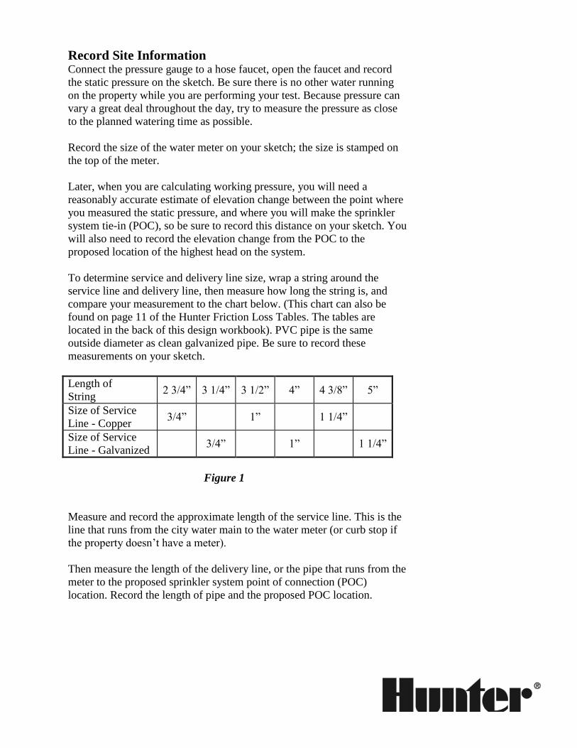
To determine service and delivery line size, wrap a string around the
service line and delivery line, then measure how long the string is, and
compare your measurement to the chart below. (This chart can also be
found on page 11 of the Hunter Friction Loss Tables. The tables are
located in the back of this design workbook). PVC pipe is the same
outside diameter as clean galvanized pipe. Be sure to record these
measurements on your sketch.
Length of
String
2 3/4”
3 1/4”
3 1/2”
4”
4 3/8”
5”
Size of Service
Line - Copper
3/4”
1”
1 1/4”
Size of Service
Line - Galvanized
3/4”
1”
1 1/4”
Figure 1
Measure and record the approximate length of the service line. This is the
line that runs from the city water main to the water meter (or curb stop if
the property doesn’t have a meter).
Then measure the length of the delivery line, or the pipe that runs from the
meter to the proposed sprinkler system point of connection (POC)
location. Record the length of pipe and the proposed POC location.
10 ft.
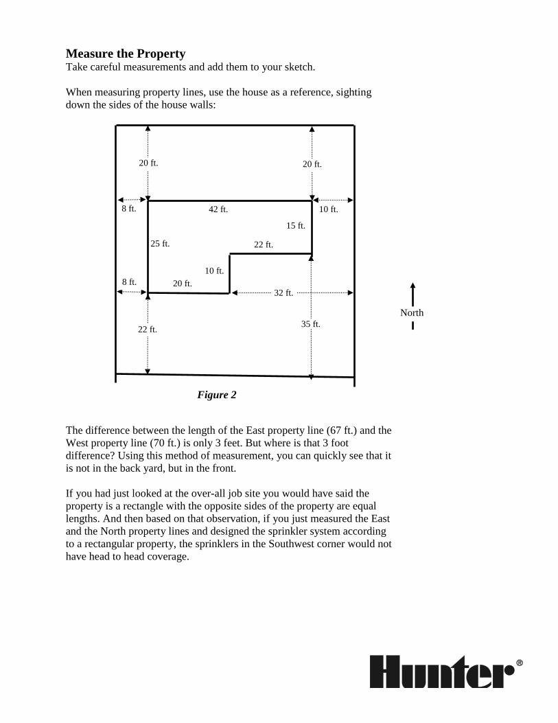
Measure the Property Take careful measurements and add them to your sketch.
When measuring property lines, use the house as a reference, sighting
down the sides of the house walls:
Figure 2
The difference between the length of the East property line (67 ft.) and the
West property line (70 ft.) is only 3 feet. But where is that 3 foot
difference? Using this method of measurement, you can quickly see that it
is not in the back yard, but in the front.
If you had just looked at the over-all job site you would have said the
property is a rectangle with the opposite sides of the property are equal
lengths. And then based on that observation, if you just measured the East
and the North property lines and designed the sprinkler system according
to a rectangular property, the sprinklers in the Southwest corner would not
have head to head coverage.
20 ft.
15 ft.
25 ft.
8 ft.
8 ft.
20 ft.
20 ft.
22 ft.
42 ft.
32 ft.
North
10 ft.
35 ft. 22 ft.
You could change the nozzle sizes and probably reach the additional 3
feet, but that may cause the system to exceed design capacity, so you may
need to add a valve, add pipe, and install a larger controller than what you
included in your bid.
You can see how sighting down the line of the wall of a house, then
continuing that imaginary line to the property line, and finally measuring
the distance from the house to the property line along that imaginary line
can be a very accurate way to set the house on the property. At the same
time, this method establishes the right locations for the property lines, and
ultimately the right locations for the sprinkler heads.
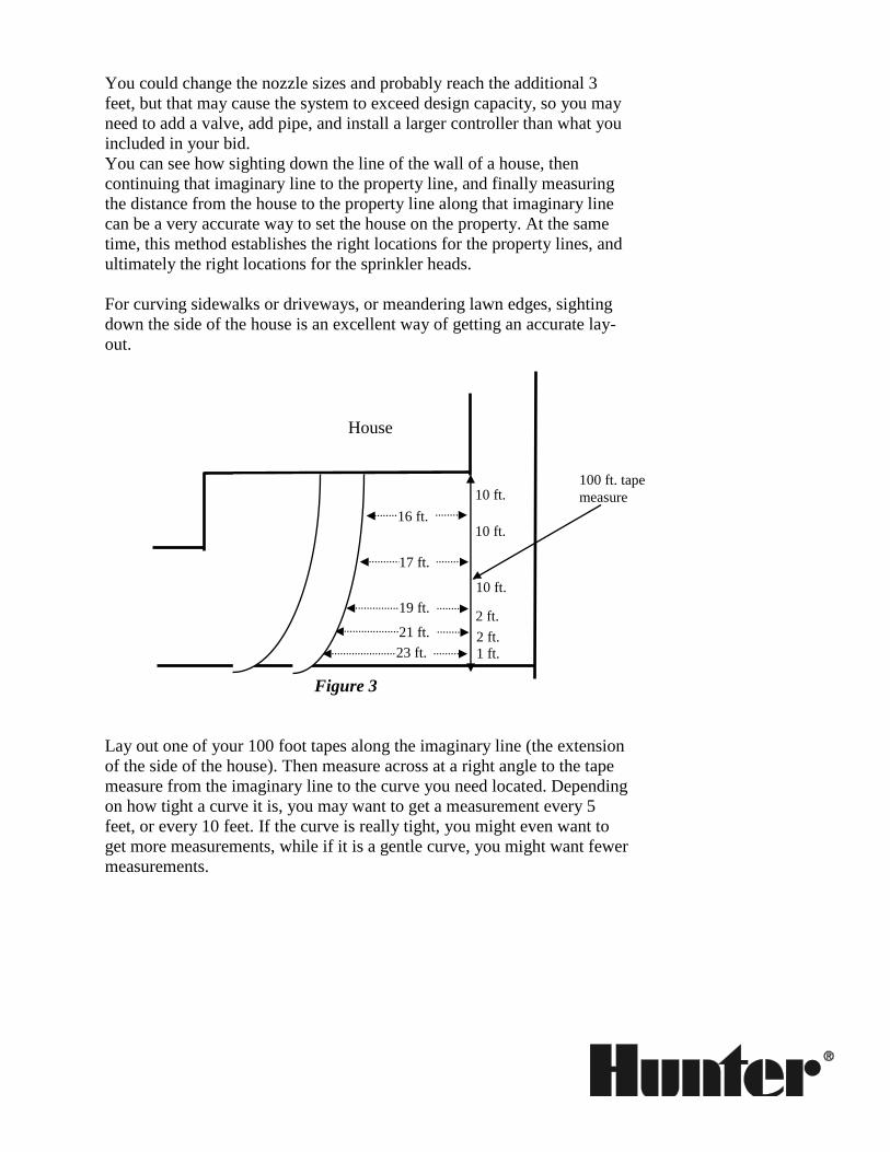
For curving sidewalks or driveways, or meandering lawn edges, sighting
down the side of the house is an excellent way of getting an accurate lay-
out.
Figure 3
Lay out one of your 100 foot tapes along the imaginary line (the extension
of the side of the house). Then measure across at a right angle to the tape
measure from the imaginary line to the curve you need located. Depending
on how tight a curve it is, you may want to get a measurement every 5
feet, or every 10 feet. If the curve is really tight, you might even want to
get more measurements, while if it is a gentle curve, you might want fewer
measurements.
100 ft. tape
measure 10 ft.
10 ft.
10 ft.
2 ft.
2 ft.
1 ft.
16 ft.
17 ft.
19 ft.
21 ft.
23 ft.
House
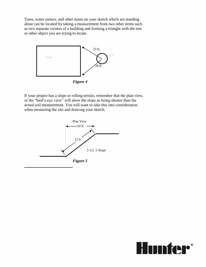
Trees, water meters, and other items on your sketch which are standing
alone can be located by taking a measurement from two other items such
as two separate corners of a building and forming a triangle with the tree
or other object you are trying to locate.
23 ft.
28 ft.
Figure 4
If your project has a slope or rolling terrain, remember that the plan view,
or the “bird’s-eye view” will show the slope as being shorter than the
actual soil measurement. You will want to take this into consideration
when measuring the site and drawing your sketch.
Figure 5
1-1/2 :1 Slope
12 ft
10 ft
Plan View
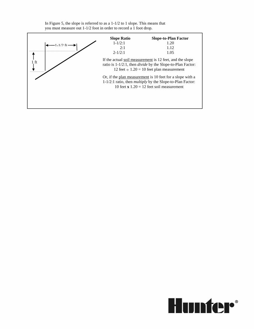
In Figure 5, the slope is referred to as a 1-1/2 to 1 slope. This means that
you must measure out 1-1/2 foot in order to record a 1 foot drop.
1 ft
1-1/2 ft
Slope Ratio Slope-to-Plan Factor
1-1/2:1 1.20
2:1 1.12
2-1/2:1 1.05
If the actual soil measurement is 12 feet, and the slope
ratio is 1-1/2:1, then divide by the Slope-to-Plan Factor:
12 feet ÷ 1.20 = 10 feet plan measurement
Or, if the plan measurement is 10 feet for a slope with a
1-1/2:1 ratio, then multiply by the Slope-to-Plan Factor:
10 feet x 1.20 = 12 feet soil measurement

Step 2 - Redraw On Graph Paper The next step is to redraw your sketch on graph paper. Be sure the
drawing is large enough to read, is positioned correctly, and fits on the
paper.
Using your drafting scale, see which scale will provide the largest drawing
possible. (Generally, the 10 or 20 scale works fine.) In the drawing in
figure 2, the longest property line is 70 feet, so you would first try the 10
scale and see if the 70 foot property line will fit on the paper. If when
using the 10 scale the property won’t fit, try the 20 scale.
Normally, you would want to position the property on the drawing so that
the North arrow is pointing up (North would be at the top of the page), and
the title block on the graph paper is to the right. In some cases, the
property will be very narrow and long with the North arrow running
parallel to the long property line. In a case such as this, you may have to
turn the property so that the North arrow is pointing side-ways in order to
use a scale where the drawing will be legible.
Be sure to transfer all of the information on your sketch to the new
drawing, including the house, property lines, driveway, trees, shrubs,
patios, decks, lawns, lamp posts, fences, walls, walkways, etc.
Once you have transferred the site information you will have a completed
plot plan on which you will be able to design your system. On the new
drawing, divide the property into areas. The areas should be as large as
possible, while considering the different watering needs of lawns and
shrubs in sunny or shady areas.
Step 3 - Select and Place Sprinklers
You are now ready to begin selecting and placing sprinklers in the
established areas. While there will be a thorough discussion of selecting
and placing sprinklers in two later sections, here is an overview of the
process:
Selecting Sprinklers Sprinkler selection is a matter of wading through the various sprinkler
characteristics and choosing the sprinkler that best suits the area you wish
to water. This information is found in the product catalog.
Information that will be important in your selection includes the
sprinkler’s operating pressure, flow range, and precipitation rate, and its
radius and arc of coverage. Additionally, each sprinkler has special
features (such as built-in check valves, side inlets, angles of trajectory)
which may be an instrumental part of the selection process.
Placing Sprinklers Begin placing sprinklers on the plan one area at a time. Start by placing
the sprinklers in the corners of the area. Be sure to draw the sprinkler’s arc
of coverage to insure head-to-head coverage.
To draw the sprinkler’s arc of coverage, set your compass to the
recommended radius according to the scale of the plot plan, and with the
pointed end on the location of the sprinkler, draw an arc. This arc should
touch or go beyond the sprinkler next to it in order to achieve head -to-
head coverage. If the arc does not reach the next head, add sprinklers
along the perimeters. Then, if necessary for full coverage, add sprinklers
in the middle.

Symbols
In order to distinguish between the sprinklers and valves and the other
products that you will be placing on the plan, you will need to draw
different symbols designating the various items.
The American Society of Irrigation Consultants (ASIC) and the American
Society of Agricultural Engineers (ASAE) have both proposed
standardized symbols for landscape irrigation. The irrigation industry,
however, has been reluctant to accept any set of standard symbols for
irrigation design.
Because of a lack of standardized symbols, many designers use some of
the proposed symbols along with symbols they have designed. In the case
of sprinkler heads, some designers have adopted a system of a circle with
an number inside. This works particularly well where sprinklers have
multiple nozzle options. The following are some suggestions for typical
symbols:
Sprinkler Heads Quarter
Half
Full
Automatic Control Valves
Isolation Valves
Controller
Lateral Line Pipe
Main Line Pipe
Symbols, no matter who designs them, should be easy to draw by hand,
and should be easily distinguishable from one to another.
Step 4 - Group Sprinklers Into Zones After you have selected and placed the sprinklers, you will need to group
them by area into zones based on the system’s design capacity.
The Design Capacity section of this Design workbook will provide you
with information on system capacity, and the System Layout section will
explain how to use that information to divide the area into separate
sprinkler zones.
To group the sprinklers into zones, write individual sprinkler GPM
requirement next to each sprinkler in the area. Add up the GPM
requirements for all sprinklers in one area, and divide by the total GPM so
that the design capacity is not exceeded.
After the individual sprinkler zones have been established, connect the
sprinklers together with pipe, size the pipe, and layout and size the valves
and backflow preventer.
Step 5 - Size Pipe and Recalculate Friction Losses To size the pipe, start at the last head on the zone and note the GPM
requirement for that head. Refer to the Hunter Friction Loss Tables for the
type of pipe you are using. Size the pipe according to the chart, then move
to the next pipe.
Add the GPM requirements of the next head to that of the last head on the
system together to size the pipe supplying the two heads.
To size the next pipe, add the GPM requirement of the next head to the
last total. Continue to do this until you get to the zone valve. Be sure to not
size a pipe smaller than the chart indicates.
After the pipes in all of the zones in all areas have been sized, refer to the
pressure loss chart in the product catalog for the valve you are using. Size
the valve according the those charts. Then size the main line pipe
according to the amount of flow needed by the zone control valves.
When you have completed the layout and pipe sizing, go back over your
design and calculate the friction loss on the most critical zones. A
thorough discussion of friction loss calculations is discussed in the
Friction Loss section.
More information on pipe layout and sizing is available in the System
Layout section.
Step 6 - Finalize Plan
Make sure the drawing is dated and if any changes are made, be sure the
date with a brief statement of those changes get noted on the plan. If your
final drawing includes more than one page, include the page numbers with
the total number of pages on all sheets (1 of 1, 1 of 3).
Irrigation designers will want to also include the following items on their
plans:
Installation details (Hunter LIT-141)
General and specific installation notes
Requirements for design or specification changes
Statement of design capacity and working pressure, for example: “This
design is based on ____ PSI at ____ GPM.”
Summary The importance of an accurate irrigation plan cannot be over stated. An
inaccurate design could mean poor coverage or lost profits. In addition to
accuracy, the completed design should be neat and include all information.
What You Need to Know While no two designers will develop a drawing the same, the following
step-by-step outline will help you in completing your sprinkler system
designs.
Step 1 - Sketch Property Sketch the property on a piece of paper
Place the house location on your sketch
Draw all concrete or brick walks, patios, and driveways
Include wood decks and their approximate height above grade
Locate walls and fences on the sketch, and note their heights
Mark the lawn areas and the locations, types, and sizes of all trees and
shrubs
Note the location of severe grade changes
Be sure to include plenty of measurements
Note the direction of North on your sketch
Take a static PSI measurement and write it on the sketch
Note the location of the water meter
Write down the sizes and the types of pipe for the service and delivery
lines
Note where you will probably make your Point of Connection (POC)
Step 2 - Redraw On Graph Paper On a separate sheet of paper, re-draw your sketch to scale
Be sure to include all walks, patios, decks, driveways, and landscape
Write the scale you are using on the plan; you do not need to include
measurements
Place the North arrow on the plot plan
Group like-landscape areas together
Step 3 - Select and Place Sprinklers Select sprinklers
Begin placing sprinklers on the plan one area at a time
Start with placing sprinklers in the corners
Draw sprinkler coverage arcs to insure head-to-head coverage
Add sprinklers along the perimeters to obtain head-to-head coverage
Add sprinklers in the middle if necessary

Step 4 - Group Sprinklers Into Zones Group sprinklers into zones
• Draw a line connecting all sprinklers on each zone
• Determine valve manifold locations
Draw a line connecting the sprinklers to zone valve
Add the main line connecting the valves to the backflow preventer and
the POC
Step 5 - Size Pipe and Recalculate Friction Losses
• Size the pipes
• Start at the last head on the zone
Size the pipe between each head adding the GPM requirements as you
go
Calculate the friction loss on the most critical zones
Step 6 - Finalize Plan Add the irrigation legend to the plan
Include any installation or other important notes
Complete the title block

On-Site Checklist
Location of trees, shrubs, other obstructions
Static Water Pressure
Water Meter Size
Elevation Change - from location of the static pressure measurement to
the POC
Elevation Change - from the POC to the where the highest head will be
located
Service Line Size, Length, and Type of Pipe
Delivery Line Size, Length, and Type of Pipe
Site Measurements for Plot Plan
Location for POC
Location of 115 Volt Electrical (for controller)
Slope Locations (note elevation changes)
Soil Type(s)
North Orientation
Direction of Prevailing Wind
Landscape and Hardscape Plan
Review Local Code Requirements
Basic Hydraulics Introduction Hydraulics is defined as a branch of science that deals with the effects of
water or other liquids in motion. In this section we will study
characteristics of water – both in motion and at rest. The emphasis will be
on the relationships between flow, velocity, and pressure. With this
knowledge we will be able to determine pressure losses in pipe and
fittings, and pressures at various points in an irrigation system.
A knowledge of the basic principles of irrigation hydraulics is essential to
designing and maintaining an economical and efficient irrigation system.
Understanding the principles outlined in this section will lead to irrigation
systems that have a more uniform distribution of water and cost less to
install and maintain.
How Does Hydraulics Affect an Irrigation System? Water pressure in an irrigation system will affect the performance of the
sprinklers. If the system is designed correctly, there will be enough
pressure throughout the system for all sprinklers to operate properly.
Maintaining this pressure in the system will help to ensure the most
uniform coverage possible. While a consistent pressure is the primary
goal, it is important to achieve this at the lowest cost. With a knowledge of
hydraulics, it is possible to design a system using the smallest and
therefore least expensive components while conserving sufficient pressure
for optimum system performance.
Water Pressure
Water pressure in irrigation systems is created in two ways: 1) by using
the weight of water (such as with a water tower) to exert the force
necessary to create pressure in the system or 2) by the use of a pump (a
mechanical pressurization).
In many municipal water delivery systems both of these methods may be
used to create the water pressure we have at our homes and businesses.
Water tanks use gravity to create pressure. These tanks are located on a
mountain top, tower or roof top. Because these storage tanks are located
above the homes they serve, the weight of the water creates pressure in the
pipes leading to those homes. In other cases, a “booster” pump is used to
increase the pressure where the elevation of the water storage tank is not
high enough above the home to provide sufficient pressure. In other areas,
the water source may be a well, lake or canal with a pump generating the
pressure.
In this section, we will explore how water pressure is affected by its
weight and what happens to water pressure when water moves through
irrigation pipes.
Water pressure can be measured or expressed in several ways:
1) psi; the most commonly used method in landscape irrigation,
pounds of pressure exerted per square inch,
2) feet of head; equivalent to the pressure at the bottom of a column of
water 1 ft. high [in this case the unit of measurement is feet of head
(ft./hd)].
How Pressure is Created By the Weight of Water What water weighs at 60° F:
• 1 cubic foot (ft.3) or 1728 cubic inches (in.3) of water = 62.43 lb.
• 1 cubic inch, (in.3) of water = 0.0361 lbs.
Water creates pressure in landscape irrigation systems by the accumulated
weight of the water.
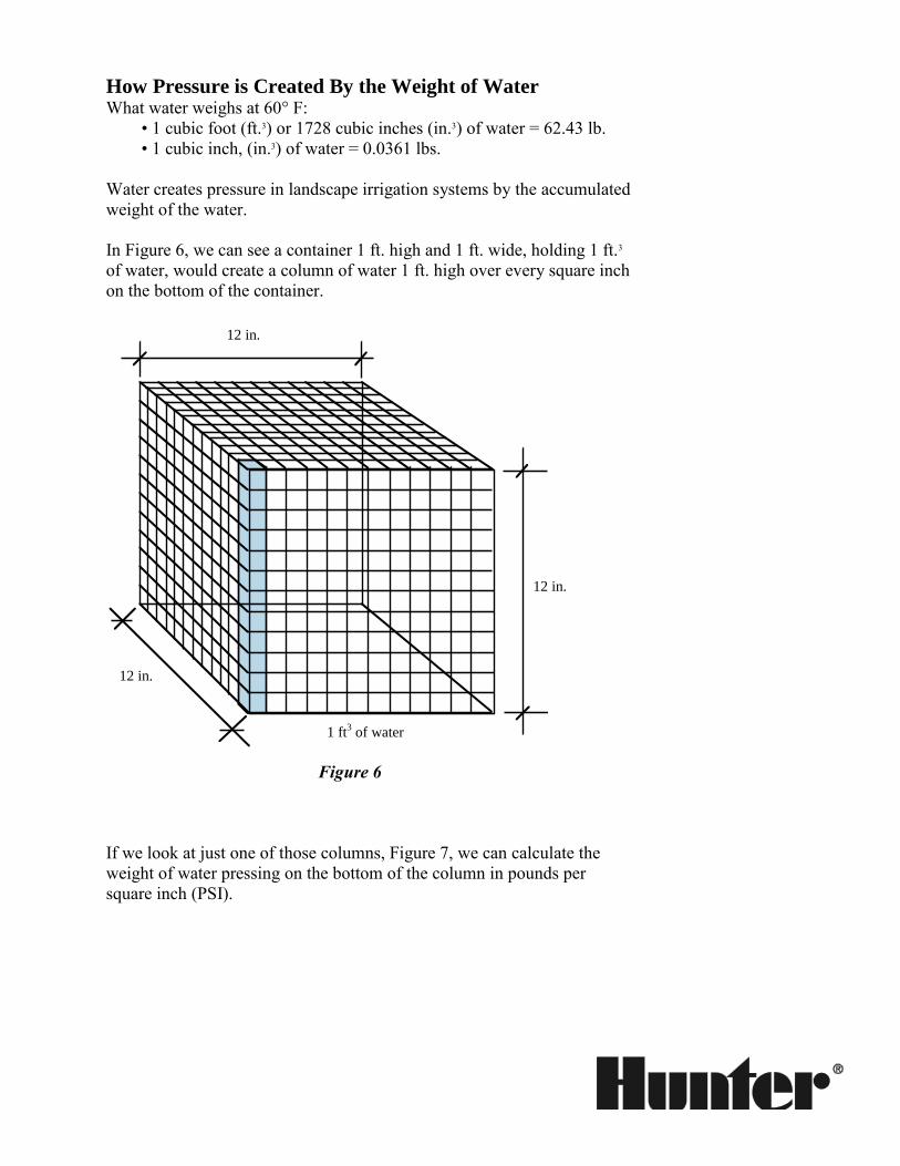
In Figure 6, we can see a container 1 ft. high and 1 ft. wide, holding 1 ft.3
of water, would create a column of water 1 ft. high over every square inch
on the bottom of the container.
Figure 6
If we look at just one of those columns, Figure 7, we can calculate the
weight of water pressing on the bottom of the column in pounds per
square inch (PSI).
12 in.
12 in.
12 in.
1 ft3 of water
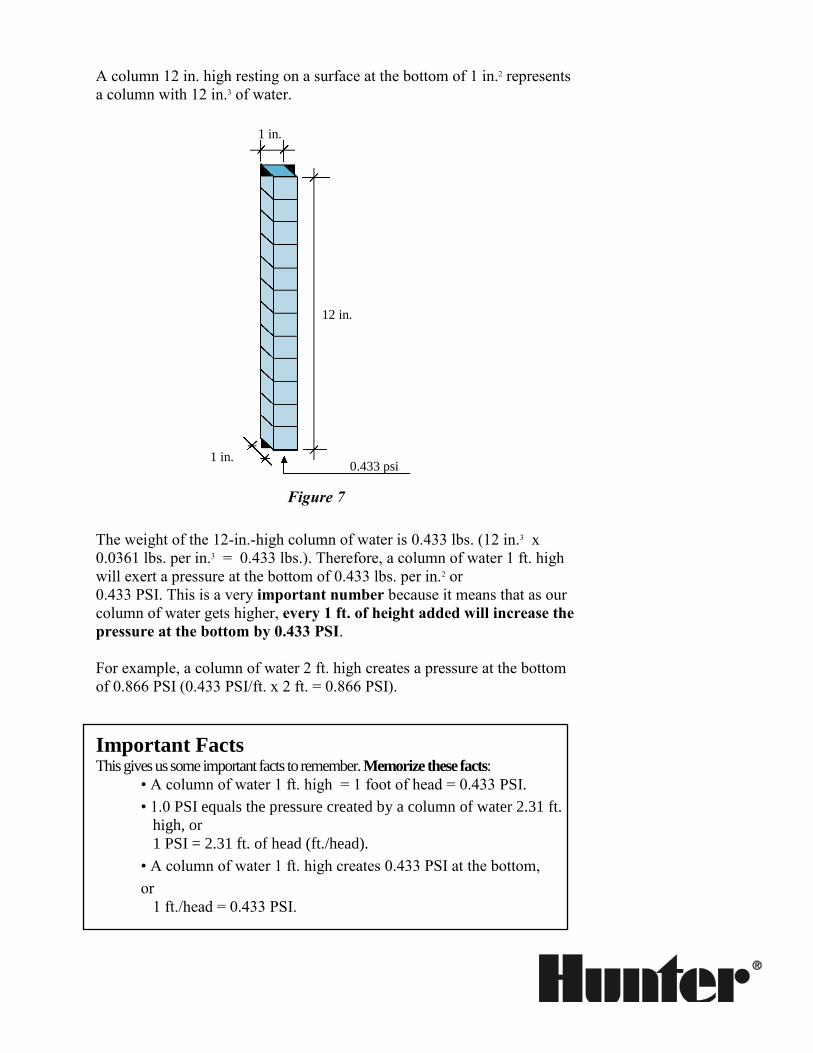
A column 12 in. high resting on a surface at the bottom of 1 in.2 represents
a column with 12 in.3 of water.
Figure 7
The weight of the 12-in.-high column of water is 0.433 lbs. (12 in.3 x
0.0361 lbs. per in.3 = 0.433 lbs.). Therefore, a column of water 1 ft. high
will exert a pressure at the bottom of 0.433 lbs. per in.2 or
0.433 PSI. This is a very important number because it means that as our
column of water gets higher, every 1 ft. of height added will increase the
pressure at the bottom by 0.433 PSI.
For example, a column of water 2 ft. high creates a pressure at the bottom
of 0.866 PSI (0.433 PSI/ft. x 2 ft. = 0.866 PSI).
Important Facts This gives us some important facts to remember. Memorize these facts:
• A column of water 1 ft. high = 1 foot of head = 0.433 PSI.
• 1.0 PSI equals the pressure created by a column of water 2.31 ft.
high, or
1 PSI = 2.31 ft. of head (ft./head).
• A column of water 1 ft. high creates 0.433 PSI at the bottom,
or
1 ft./head = 0.433 PSI.
1 in.
12 in.
1 in. 0.433 psi
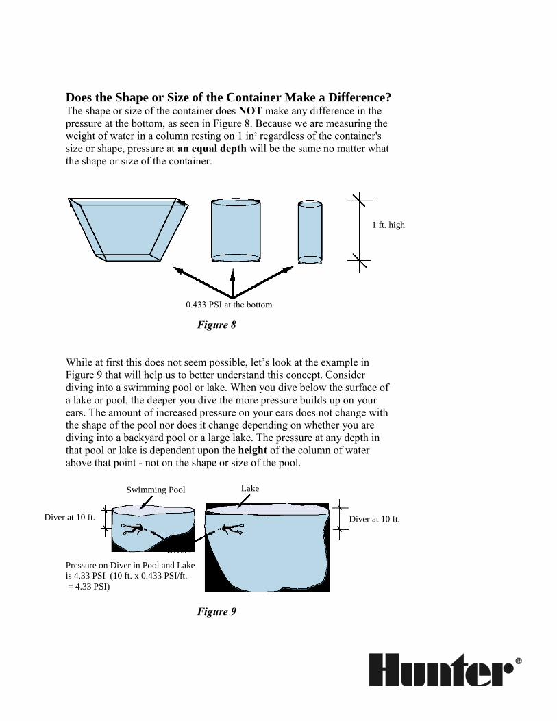
Does the Shape or Size of the Container Make a Difference? The shape or size of the container does NOT make any difference in the
pressure at the bottom, as seen in Figure 8. Because we are measuring the
weight of water in a column resting on 1 in2 regardless of the container's
size or shape, pressure at an equal depth will be the same no matter what
the shape or size of the container.
0.433 PSI at the bottom
Figure 8
While at first this does not seem possible, let’s look at the example in
Figure 9 that will help us to better understand this concept. Consider
diving into a swimming pool or lake. When you dive below the surface of
a lake or pool, the deeper you dive the more pressure builds up on your
ears. The amount of increased pressure on your ears does not change with
the shape of the pool nor does it change depending on whether you are
diving into a backyard pool or a large lake. The pressure at any depth in
that pool or lake is dependent upon the height of the column of water
above that point - not on the shape or size of the pool.
Figure 9
1 ft. high
Diver at 10 ft. Diver at 10 ft.
Pressure on Diver in Pool and Lake
is 4.33 PSI (10 ft. x 0.433 PSI/ft.
= 4.33 PSI)
Swimming Pool Lake
Divers
What Does This Mean in Irrigation Design? When designing landscape irrigation systems, for every 1 ft. of elevation
change there will be a corresponding change in pressure of 0.433 PSI.
Static and Dynamic Pressure There are two classifications of water pressure:
static and dynamic pressure:
• Static pressure is a measurement of water pressure when the
water is at rest. In other words, the water is not moving in the
system.
• Dynamic pressure (or working pressure) is a measurement of
water pressure with the water in motion (also known as
working pressure).
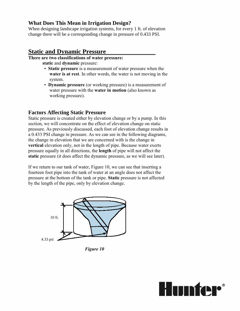
Factors Affecting Static Pressure Static pressure is created either by elevation change or by a pump. In this
section, we will concentrate on the effect of elevation change on static
pressure. As previously discussed, each foot of elevation change results in
a 0.433 PSI change in pressure. As we can see in the following diagrams,
the change in elevation that we are concerned with is the change in
vertical elevation only, not in the length of pipe. Because water exerts
pressure equally in all directions, the length of pipe will not affect the
static pressure (it does affect the dynamic pressure, as we will see later).
If we return to our tank of water, Figure 10, we can see that inserting a
fourteen foot pipe into the tank of water at an angle does not affect the
pressure at the bottom of the tank or pipe. Static pressure is not affected
by the length of the pipe, only by elevation change.
Figure 10
10 ft.
4.33 psi
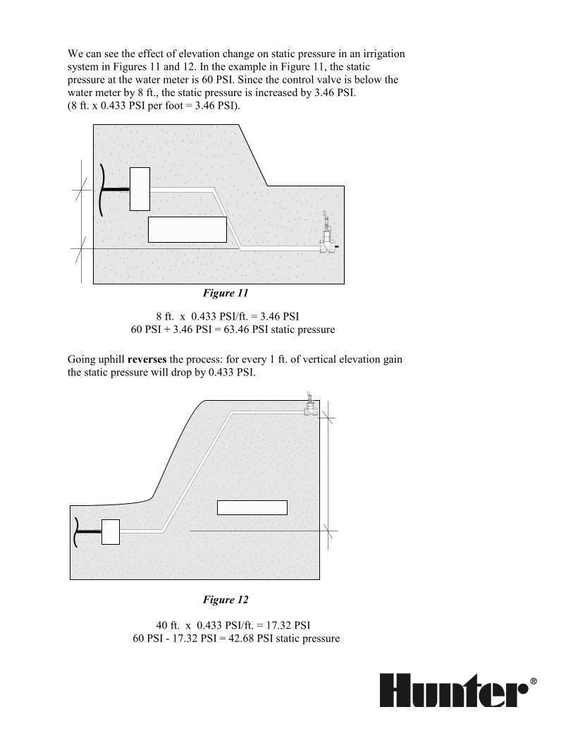
We can see the effect of elevation change on static pressure in an irrigation
system in Figures 11 and 12. In the example in Figure 11, the static
pressure at the water meter is 60 PSI. Since the control valve is below the
water meter by 8 ft., the static pressure is increased by 3.46 PSI.
(8 ft. x 0.433 PSI per foot = 3.46 PSI).
Figure 11
8 ft. x 0.433 PSI/ft. = 3.46 PSI
60 PSI + 3.46 PSI = 63.46 PSI static pressure
Going uphill reverses the process: for every 1 ft. of vertical elevation gain
the static pressure will drop by 0.433 PSI.
Figure 12
40 ft. x 0.433 PSI/ft. = 17.32 PSI
60 PSI - 17.32 PSI = 42.68 PSI static pressure
24 VAC
60mA
60mA
50-60 Hz
INRUSH
HOLDING
OFF ON
SO LEN O ID
LO W C U R R E NT
24 VAC
60mA
60mA
50-60 Hz
INRUSH
HOLDING
OFF ON
SO LE N O ID
L O W C U R RE N T
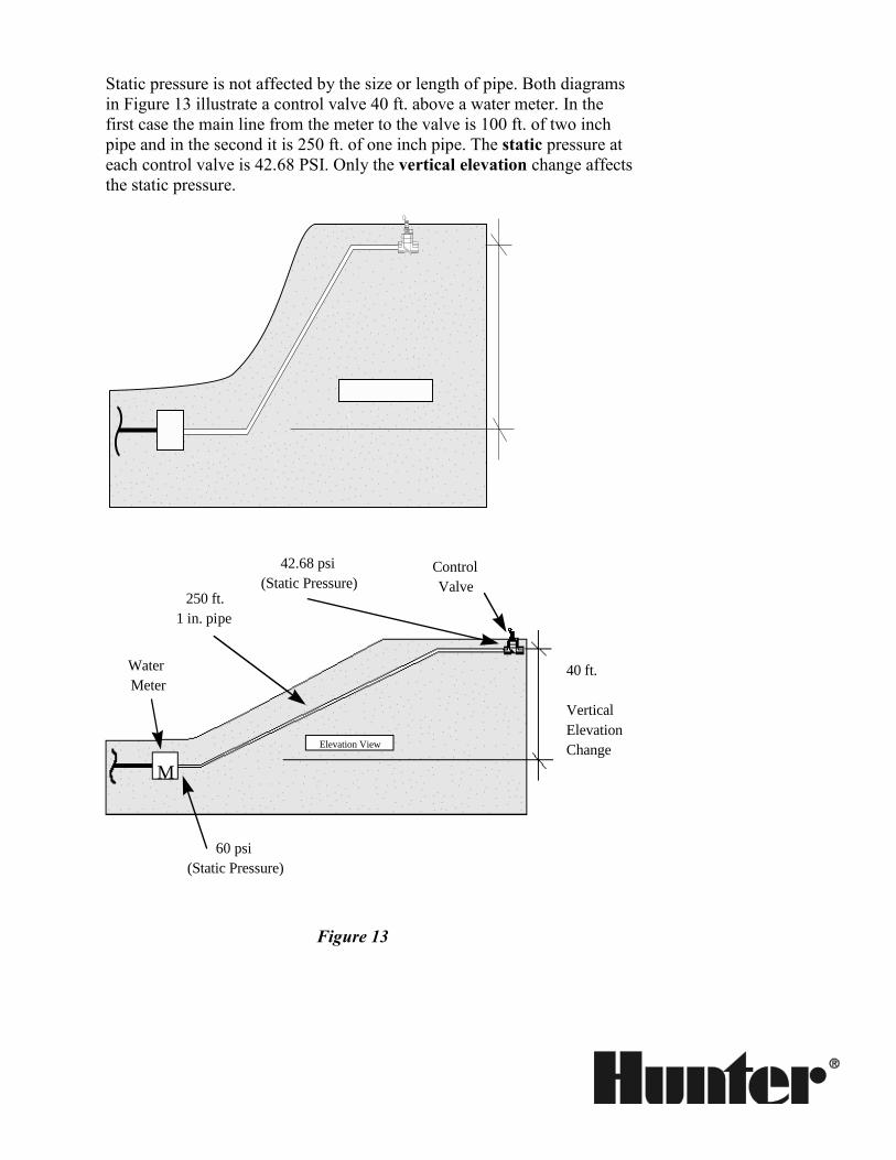
Static pressure is not affected by the size or length of pipe. Both diagrams
in Figure 13 illustrate a control valve 40 ft. above a water meter. In the
first case the main line from the meter to the valve is 100 ft. of two inch
pipe and in the second it is 250 ft. of one inch pipe. The static pressure at
each control valve is 42.68 PSI. Only the vertical elevation change affects
the static pressure.
Water
Meter
250 ft.
1 in. pipe
40 ft.
Vertical
Elevation
Change
60 psi
(Static Pressure)
42.68 psi
(Static Pressure) Control
Valve
M
Elevation View
Figure 13
24 VAC
60mA
60mA
50-60 Hz
INRUSH
HOLDING
OFF ON
S O LE NO ID
LO W C U R R EN T
Factors Affecting Dynamic Pressure When water moves through an irrigation system it is said to be in a
dynamic state. The movement of water is described in terms of velocity
(the speed at which it is moving) and flow (the amount of water moving
through the system). The velocity is measured in feet per second (fps) and
the flow is measured in gallons per minute (GPM). Dynamic water
pressure is measured in the same units as static pressure (PSI).
Dynamic pressure is affected by the following factors:
1) change in elevation (change in elevation affects static and dynamic
pressure in the same way)
2) friction losses in pipe, valves and fittings (pressure loss is caused
by water moving through the system)
3) velocity head (the pressure required to make water move within the
system; this is a minor loss and won’t be calculated here)
4) entrance losses (the pressure lost as water flows through openings;
this is also a minor loss and won’t be calculated here)
Friction Loss in Pipe When measuring dynamic pressure at any point in a landscape irrigation
system, we must first determine the static pressure at that point and then
subtract the pressure losses due to the movement of water.
As water moves through an irrigation system, pressure is lost because of
turbulence created by the moving water. This turbulence can be created in
pipes, valves or fittings. These pressure losses are referred to as “friction
losses.”
There are four factors that affect friction losses in pipe:
1) the velocity of the water,
2) the inside diameter of the pipe,
3) the roughness of the inside of the pipe and
4) the length of the pipe.
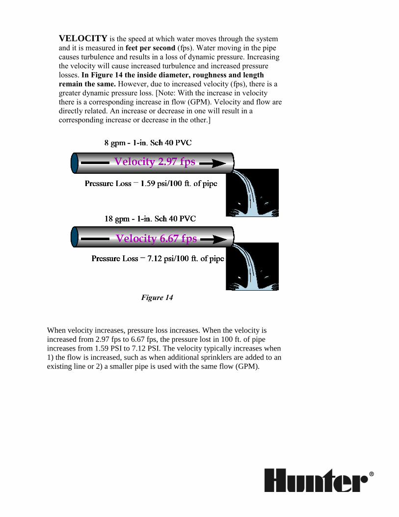
VELOCITY is the speed at which water moves through the system
and it is measured in feet per second (fps). Water moving in the pipe
causes turbulence and results in a loss of dynamic pressure. Increasing
the velocity will cause increased turbulence and increased pressure
losses. In Figure 14 the inside diameter, roughness and length
remain the same. However, due to increased velocity (fps), there is a
greater dynamic pressure loss. [Note: With the increase in velocity
there is a corresponding increase in flow (GPM). Velocity and flow are
directly related. An increase or decrease in one will result in a
corresponding increase or decrease in the other.]
Figure 14
When velocity increases, pressure loss increases. When the velocity is
increased from 2.97 fps to 6.67 fps, the pressure lost in 100 ft. of pipe
increases from 1.59 PSI to 7.12 PSI. The velocity typically increases when
1) the flow is increased, such as when additional sprinklers are added to an
existing line or 2) a smaller pipe is used with the same flow (GPM).
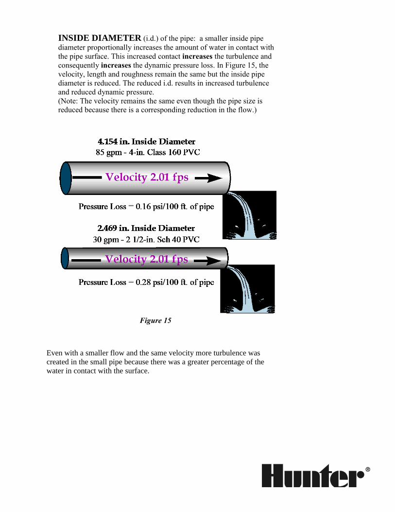
INSIDE DIAMETER (i.d.) of the pipe: a smaller inside pipe
diameter proportionally increases the amount of water in contact with
the pipe surface. This increased contact increases the turbulence and
consequently increases the dynamic pressure loss. In Figure 15, the
velocity, length and roughness remain the same but the inside pipe
diameter is reduced. The reduced i.d. results in increased turbulence
and reduced dynamic pressure.
(Note: The velocity remains the same even though the pipe size is
reduced because there is a corresponding reduction in the flow.)
Figure 15
Even with a smaller flow and the same velocity more turbulence was
created in the small pipe because there was a greater percentage of the
water in contact with the surface.
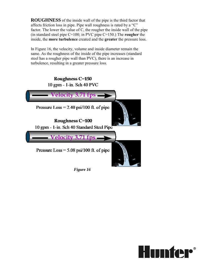
ROUGHNESS of the inside wall of the pipe is the third factor that
affects friction loss in pipe. Pipe wall roughness is rated by a “C”
factor. The lower the value of C, the rougher the inside wall of the pipe
(in standard steel pipe C=100; in PVC pipe C=150.) The rougher the
inside, the more turbulence created and the greater the pressure loss.
In Figure 16, the velocity, volume and inside diameter remain the
same. As the roughness of the inside of the pipe increases (standard
steel has a rougher pipe wall than PVC), there is an increase in
turbulence, resulting in a greater pressure loss.
Figure 16
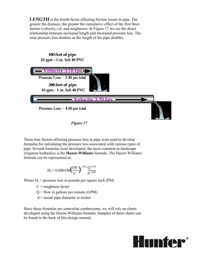
LENGTH is the fourth factor affecting friction losses in pipe. The
greater the distance, the greater the cumulative effect of the first three
factors (velocity, i.d. and roughness). In Figure 17 we see the direct
relationship between increased length and increased pressure loss. The
total pressure loss doubles as the length of the pipe doubles.
Figure 17
These four factors affecting pressure loss in pipe were used to develop
formulas for calculating the pressure loss associated with various types of
pipe. Several formulas were developed; the most common in landscape
irrigation hydraulics is the Hazen-Williams formula. The Hazen-Williams
formula can be represented as:
Hf = 0.090194( )
Where Hf = pressure loss in pounds per square inch (PSI)
C = roughness factor
Q = flow in gallons per minute (GPM)
d = inside pipe diameter in inches
Since these formulas are somewhat cumbersome, we will rely on charts
developed using the Hazen-Williams formula. Samples of these charts can
be found in the back of this design manual.
100
C
1.852 Q
d
1.852
4.866
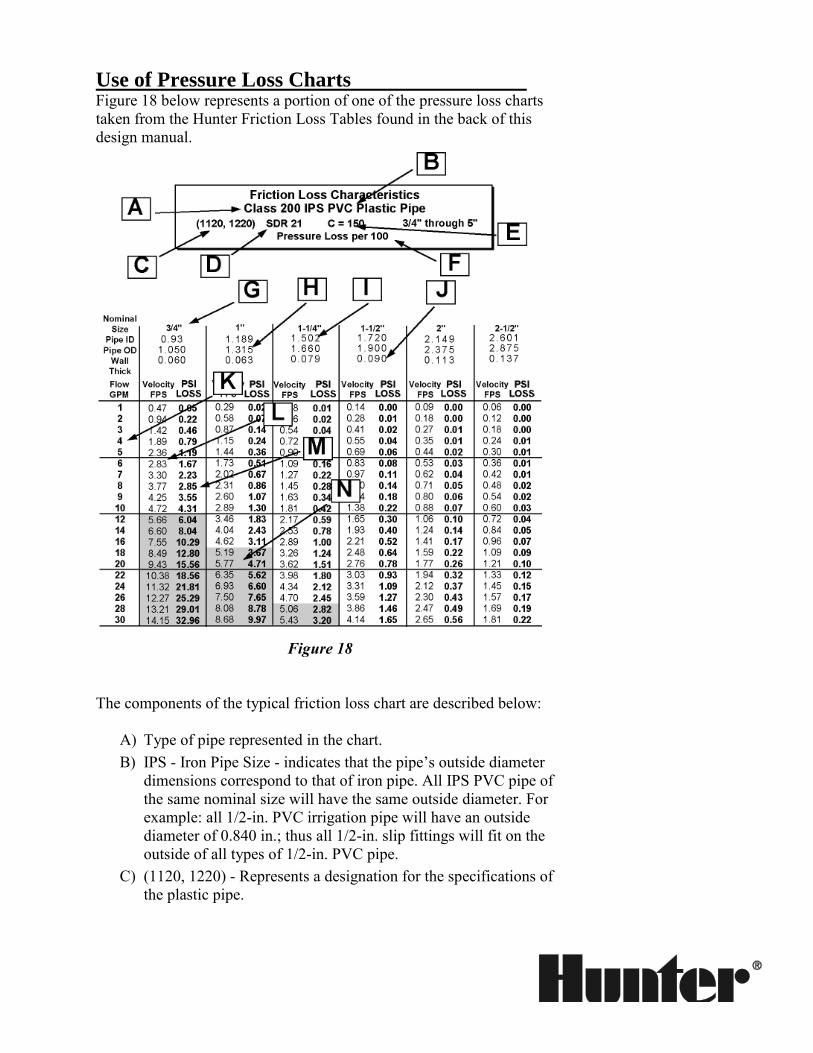
Use of Pressure Loss Charts Figure 18 below represents a portion of one of the pressure loss charts
taken from the Hunter Friction Loss Tables found in the back of this
design manual.
Figure 18
The components of the typical friction loss chart are described below:
A) Type of pipe represented in the chart.
B) IPS - Iron Pipe Size - indicates that the pipe’s outside diameter
dimensions correspond to that of iron pipe. All IPS PVC pipe of
the same nominal size will have the same outside diameter. For
example: all 1/2-in. PVC irrigation pipe will have an outside
diameter of 0.840 in.; thus all 1/2-in. slip fittings will fit on the
outside of all types of 1/2-in. PVC pipe.
C) (1120, 1220) - Represents a designation for the specifications of
the plastic pipe.
D) SDR –Standard Dimension Ratio – indicates the pipe’s wall
thickness as a ratio of the outside diameter. Outside diameter of 1-
in. pipe is 1.315 in. If you divide 1.315 by the SDR, 21, it will give
you a minimum wall thickness. (There may be some exceptions to
this rule.) Minimum wall thickness for 1-in. Class 200 PVC pipe
1.315/21=0.063 in. Class-rated pipes (SDR pipes) maintain a
uniform maximum operating pressure across all pipe sizes. This is
not true of schedule rated pipes such as Schedule 40 PVC. In
schedule rated pipes the maximum operating pressure decreases as
pipe size increases.
E) C=150 – indicates the value of the C factor, which is a measure of
the roughness of the inside of the pipe. The lower the number, the
rougher the inside of the pipe and the greater the pressure loss. For
PVC, C = 150; Galvanized Pipe C = 100.
F) Designated pressure losses shown in the chart are per 100 ft.
of pipe.
G Size – indicates the “nominal” pipe size. Nominal means “in name
only,” and none of the actual pipe dimensions are exactly that size.
For example, in the 3/4-in. pipe, none of the dimensions are actually 3/4-in.
H) OD – outside pipe diameter in inches.
I) ID – inside pipe diameter in inches.
J) Wall Thick – wall thickness in inches.
K) Flow (GPM) – flow rate in gallons per minute.
L) Velocity (fps) – speed of water in feet per second at the
corresponding flow rate.
M) PSI Loss – pressure loss per 100 ft. of pipe in pounds per square
inch at the corresponding flow rate.
N) The shaded area on the chart designates those flow rates that
exceed 5 fps. It is recommended that caution be used with flow
rates above 5 fps in main lines where water hammer will be a
concern.
What the Charts Are Used for These charts are used to:
• Determine the pressure loss in pipe due to friction losses
• Determine the velocity at various flow rates
• Use pressure losses and/or velocities to determine appropriate
pipe sizes (pipe sizing is covered in another section)
How to Use the Friction Loss Charts to Calculate Loss in a
Specific Length of Pipe Using the Hunter Friction Loss Tables in the back of this design manual:
1. Find the flow of water in gallons per minute (GPM) in the column
on the left.
2. Now read across the top of the chart looking for the size of the
pipe.
3. Read down this column, under the “PSI Loss” heading, and across
the row for the GPM.
4. Divide this number by 100 to find the PSI loss per foot.
5. Multiply this number times the length of the pipe in feet.
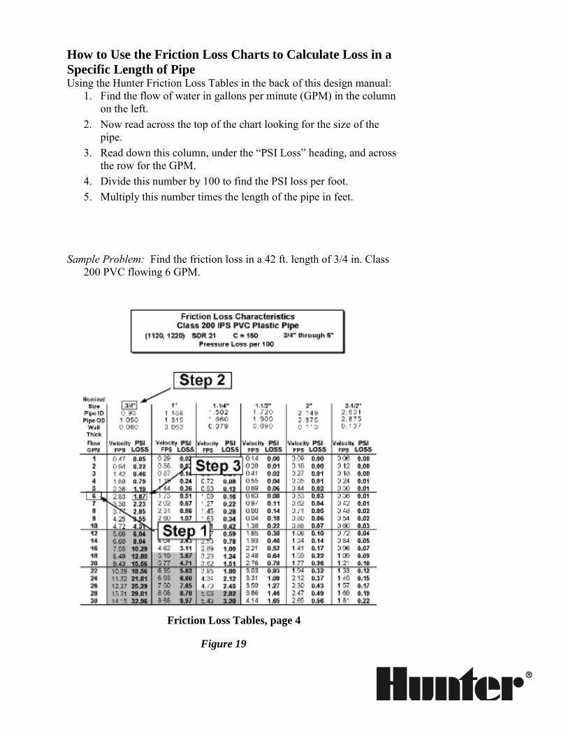
Sample Problem: Find the friction loss in a 42 ft. length of 3/4 in. Class
200 PVC flowing 6 GPM.
Friction Loss Tables, page 4
Figure 19
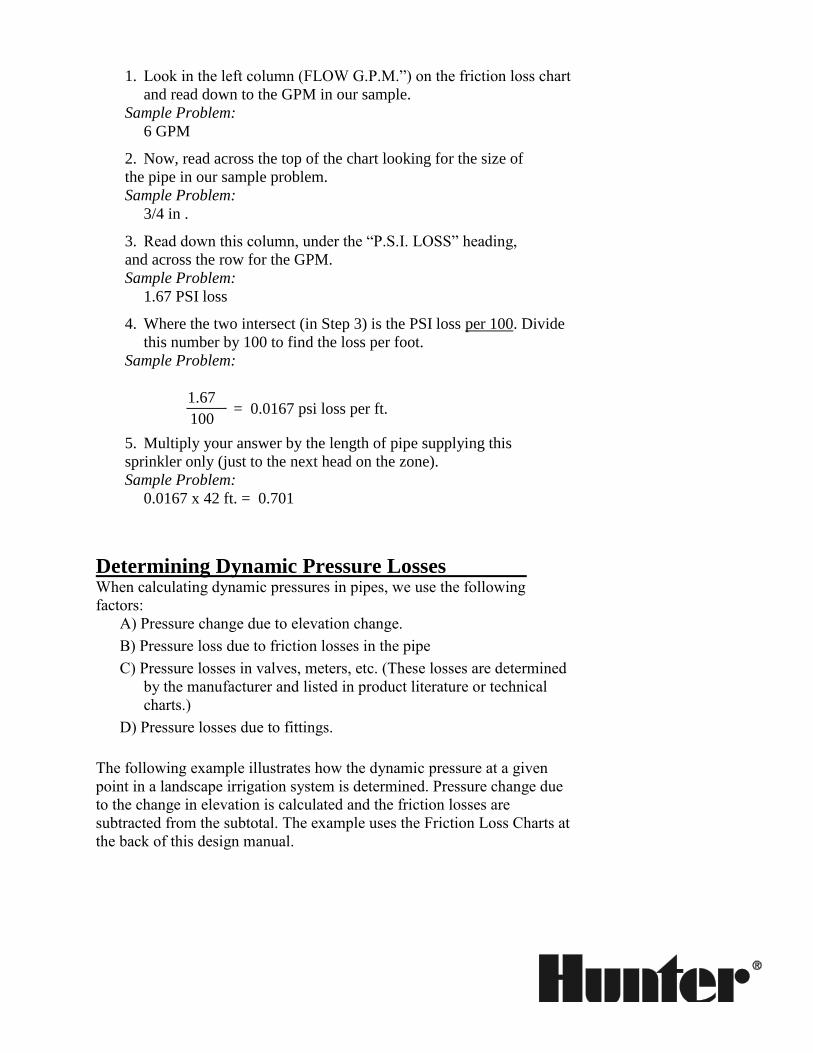
1. Look in the left column (FLOW G.P.M.”) on the friction loss chart
and read down to the GPM in our sample.
Sample Problem:
6 GPM
2. Now, read across the top of the chart looking for the size of
the pipe in our sample problem.
Sample Problem:
3/4 in .
3. Read down this column, under the “P.S.I. LOSS” heading,
and across the row for the GPM.
Sample Problem:
1.67 PSI loss
4. Where the two intersect (in Step 3) is the PSI loss per 100. Divide
this number by 100 to find the loss per foot.
Sample Problem:
5. Multiply your answer by the length of pipe supplying this
sprinkler only (just to the next head on the zone).
Sample Problem:
0.0167 x 42 ft. = 0.701
Determining Dynamic Pressure Losses When calculating dynamic pressures in pipes, we use the following
factors:
A) Pressure change due to elevation change.
B) Pressure loss due to friction losses in the pipe
C) Pressure losses in valves, meters, etc. (These losses are determined
by the manufacturer and listed in product literature or technical
charts.)
D) Pressure losses due to fittings.
The following example illustrates how the dynamic pressure at a given
point in a landscape irrigation system is determined. Pressure change due
to the change in elevation is calculated and the friction losses are
subtracted from the subtotal. The example uses the Friction Loss Charts at
the back of this design manual.
= 0.0167 psi loss per ft. 1.67
100
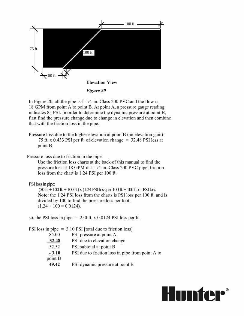
Elevation View
Figure 20
In Figure 20, all the pipe is 1-1/4-in. Class 200 PVC and the flow is
18 GPM from point A to point B. At point A, a pressure gauge reading
indicates 85 PSI. In order to determine the dynamic pressure at point B,
first find the pressure change due to change in elevation and then combine
that with the friction loss in the pipe.
Pressure loss due to the higher elevation at point B (an elevation gain):
75 ft. x 0.433 PSI per ft. of elevation change = 32.48 PSI less at
point B
Pressure loss due to friction in the pipe:
Use the friction loss charts at the back of this manual to find the
pressure loss at 18 GPM in 1-1/4-in. Class 200 PVC pipe: friction
loss from the chart is 1.24 PSI per 100 ft.
PSI loss in pipe:
(50 ft. + 100 ft. + 100 ft.) x (1.24 PSI loss per 100 ft. ÷ 100 ft.) = PSI loss
Note: the 1.24 PSI loss from the charts is PSI loss per 100 ft. and is
divided by 100 to find the pressure loss per foot,
(1.24 ÷ 100 = 0.0124).
so, the PSI loss in pipe = 250 ft. x 0.0124 PSI loss per ft.
PSI loss in pipe = 3.10 PSI [total due to friction loss]
85.00 PSI pressure at point A
- 32.48 PSI due to elevation change
52.52 PSI subtotal at point B
- 3.10 PSI due to friction loss in pipe from point A to
point B
49.42 PSI dynamic pressure at point B
Point A Point B
1-1/4 in. CL 200 PVC
85 psi at Point A
18 GPM
100 ft. 75 ft.
100 ft.
50 ft.
Summary
There is a limited amount of pressure helping to supply water to a sprinkler
system. As more sprinklers are added to a system, the GPM requirement
increases. As the GPM increases, the velocity of the water increases until the
pressure losses due to friction equal the pressure available at the source.
The design of a landscape irrigation system requires an understanding of
water movement. Changes in elevation and friction losses in pipe, valves,
and fittings affect pressure, which in turn affects sprinkler performance.
Irrigation hydraulics is used to determine the volume of water available
for use by the system, the pressure available at the sprinkler heads, and the
correct pipe sizes.
Understanding the principles of hydraulics outlined in this section will
lead to irrigation systems that have a more uniform distribution of water
and cost less to install and maintain.
What You Need to Know
Water pressure is created by:
weight of water
pump (mechanical pressurization)
Water pressure can be measured in:
PSI (pounds per square inch)
ft./hd. (feet of head)
For every one foot of elevation change, the water pressure:
Increases 0.433 PSI going downhill from the P.O.C.
Decreases 0.433 PSI going uphill from the P.O.C.
Design Capacity
Introduction The two questions that most frequently confuse someone learning
irrigation system design are, 1) “How much water will be available for
my irrigation system?” and, 2) “What pressure will I have available for
my sprinklers?”
The reason there is so much confusion surrounding this topic is that there
are many factors affecting how much water will be available (Design
Capacity), and what the pressure will be at the sprinkler head (Dynamic,
or Working Pressure); the static pressure at the source, net elevation
change, the size and length of the service line and delivery line, water
meter size, filters, backflow prevention devices, and the number and size
of gate valves. While many texts and references refer to “restricting flows
to conserve pressure”, or list “restrictions on appropriate flows”, most fail
to offer an orderly, step-by-step method to answering these two basic
questions.
This section will explain how to determine the flow available for use in
the sprinkler system and what pressure can be expected for sprinkler
operation.
Determining Water Supply and Available Pressure How to calculate the flow or design capacity and the dynamic pressure
available will vary depending upon the water source. This section is
divided into three parts depending on the water source:
I. Metered Municipal Water Sources (page 38)
II. Unmetered Municipal Water Sources (page 51)
III. Pump Delivered Well Sources (page 52)
.
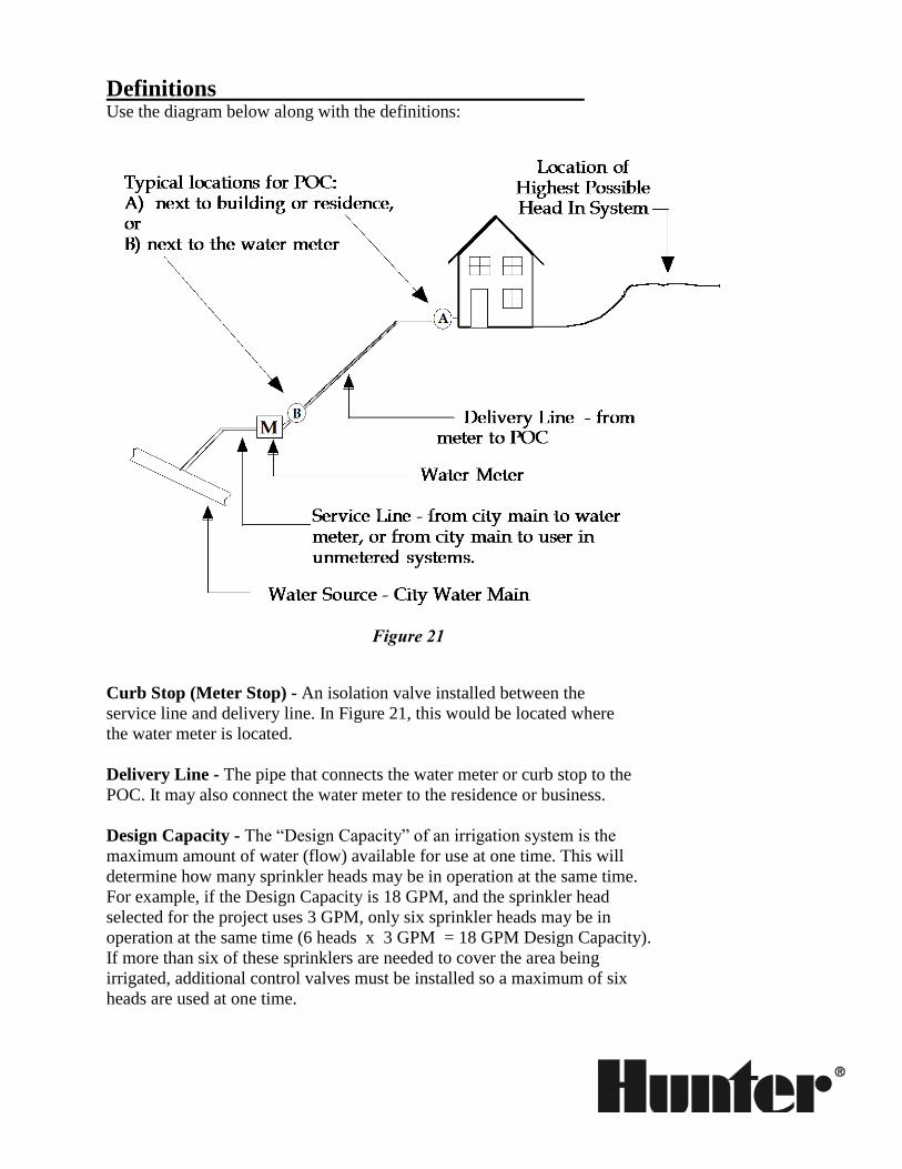
Definitions Use the diagram below along with the definitions:
Figure 21
Curb Stop (Meter Stop) - An isolation valve installed between the
service line and delivery line. In Figure 21, this would be located where
the water meter is located.
Delivery Line - The pipe that connects the water meter or curb stop to the
POC. It may also connect the water meter to the residence or business.
Design Capacity - The “Design Capacity” of an irrigation system is the
maximum amount of water (flow) available for use at one time. This will
determine how many sprinkler heads may be in operation at the same time.
For example, if the Design Capacity is 18 GPM, and the sprinkler head
selected for the project uses 3 GPM, only six sprinkler heads may be in
operation at the same time (6 heads x 3 GPM = 18 GPM Design Capacity).
If more than six of these sprinklers are needed to cover the area being
irrigated, additional control valves must be installed so a maximum of six
heads are used at one time.
Dynamic Pressure - The available dynamic pressure, also known as working
pressure, is simply the water pressure calculated while the water is flowing.
The “Dynamic Pressure at Design Capacity” is a calculation of the pressure
(PSI) available at the maximum system flow rate. This pressure is calculated
at the system Point of Connection (POC). The dynamic pressure at the POC
will influence your choice of sprinkler heads. For example, you would not
choose a head with an operating pressure rating that is above the available
dynamic pressure
Estimated Dynamic Pressure at Worst Case Head - Once the Dynamic
Pressure at Design Capacity is calculated, an estimate is made of the pressure
that will be available for the sprinklers. The “Worst Case Head” indicates this
head is the highest head in the system. The Design Capacity (GPM) and
Estimated Dynamic Pressure at Design Capacity (PSI) are used to select the
sprinklers. Pressure and flow limitations are two of the prime factors in
sprinkler selection.
Flow - The volume/velocity rate water moving through a system. This can be
measured in gallons per minute (GPM), gallons per hour (gph), liters per
second (l/s), liters per minute (l/min), or cubic meters per hour (m3/hr).
Point of Connection - The Point of Connection (POC) is where the irrigation
system is connected to the water source. This represents a logical or
convenient location to connect the irrigation system to the water supply.
Service Line - The service line is the pipe connection between the city main
in the street and the water meter. In the case of unmetered systems, it is the
pipe between the city water main and the curb stop.
Water Meter - A device used to measure water usage. In southern climates,
the meter is usually located near the property line, close to the city main line.
In northern climates, the meter is usually in a basement or other indoor
location.
Working Pressure - See Dynamic Pressure
Calculating Dynamic Pressure at Design Capacity The following sections explain how to determine design capacity and
dynamic pressure at design capacity, and estimate the dynamic pressure
for the worst case head for the three most common landscape irrigation
water sources. The three most common water sources are: 1) metered
municipal systems, 2) unmetered municipal systems, and 3) pumping from
a well.
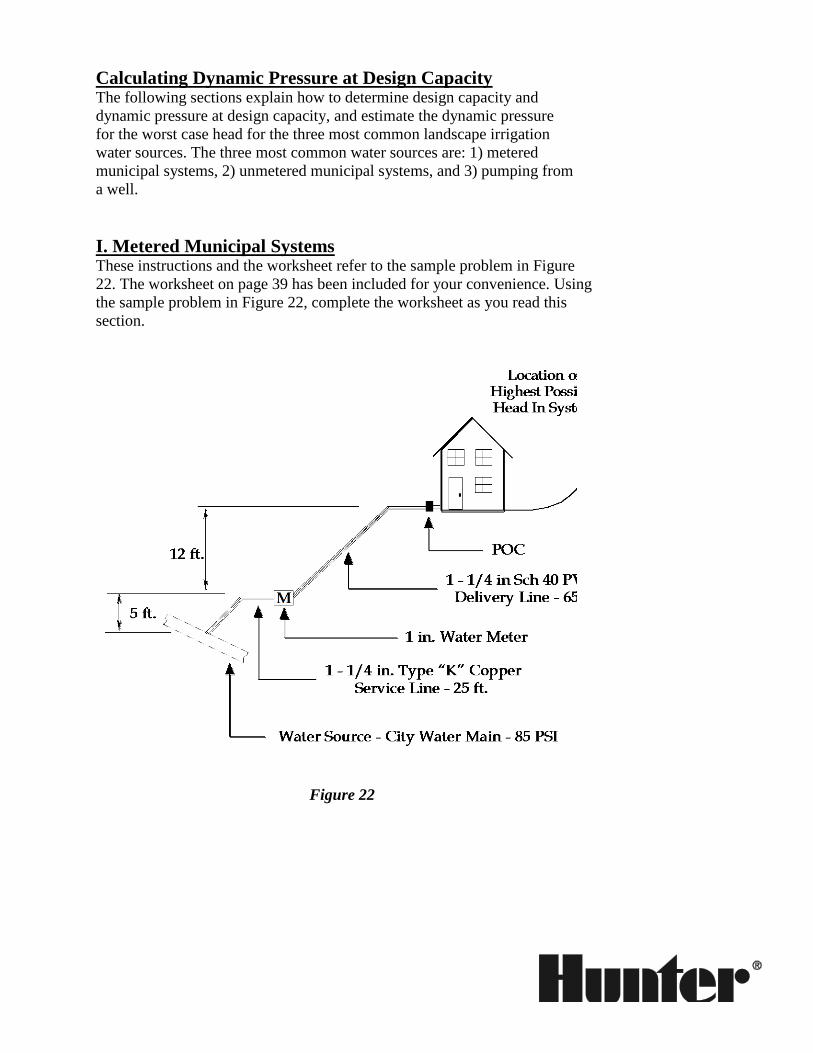
I. Metered Municipal Systems These instructions and the worksheet refer to the sample problem in Figure
22. The worksheet on page 39 has been included for your convenience. Using
the sample problem in Figure 22, complete the worksheet as you read this
section.
Figure 22

(METERED SYSTEMS)
Design Capacity and Working Pressure Worksheet
CALCULATING DESIGN CAPACITY AND DYNAMIC PRESSURE
A. Record Site Information
1 Static* Pressure at the Source (Main) PSI 2 Net elevation Change (Source to POC) ± FEET (+ uphill, - downhill) 3 Pressure change due to elevation: Line 2 x 0.433 = PSI 4 Static Pressure at POC: Line 1 +/- Line 3 = PSI Number/Length Size Type 5 Service Line 6 Delivery Line 7 Water Meter 8 Isolation Valves 9 Other
B. Determine Design Capacity GPM With Factor Restriction Restriction 10 Pressure loss through Not to exceed 10% of available the water meter. PSI at the source(Line 1) GPM 11 Volume through the Not to exceed 75% of maximum water meter. safe flow of the meter. GPM 12 Velocity through the Velocity not to exceed 7.5 fps service line. (Main to meter) GPM
13 Design Capacity Lowest GPM of the three flows rates - lines 10, 11, and
12. GPM
C. Calculate Dynamic Pressure at Design Capacity
Pressure Losses from Source(City Water Main) to the POC 14 Pressure loss in the Service Line PSI loss (per 100' ) x ft./100 = PSI 15 Pressure loss in the Delivery Line PSI loss (per 100' ) x ft./100 = PSI 16 Pressure loss in the Water Meter at design capacity = PSI 17 Pressure loss in the Gate Valves: _____ Equivalence Factor x _____ PSI loss per 100' of Standard Steel/100 x _____ Number of Gate Valves = PSI 18 Other pressure losses_____________________________ = PSI 19 Pressure loss from the source to POC (add Lines 14 through 18) PSI 20 Approximate Dynamic Pressure at Design Capacity Static Pressure at the POC (Line 4 above) PSI Subtract the PSI lost from the source to the POC (Line 19 ) PSI Approximate Dynamic Pressure at Design Capacity PSI

D. Estimate Pressure Available at “Worst-Case” Head
21 Pressure change due to elevation change from the POC to the highest head in the system. ft. x 0.433 = PSI 22 Pressure subtotal (subtract Line 21 from Line 20; for worst case heads which are lower than the POC, add Lines 20 and 21) PSI 23 Estimated Pressure Available at worst case-head two-thirds of subtotal: Line 22 PSI x 0.67 = PSI
Pressure Available for Sprinkler Selection and Operation PSI
*Although this is referred to as static pressure, in municipal systems it is taken to mean the minimum dynamic
pressure at the water main.

A. Record Site Information Line #1 - Static* Pressure at the Source: For municipal systems,
the static pressure at the source can be obtained from the water purveyor.
This is usually a municipal water utilities department, quasi-governmental
agency, or a private water company. It is suggested that this information
be obtained from the water company rather than by using a gauge because
the water company can also tell you what minimum pressure you would
expect in the main line. Service line size and type can be obtained at the
same time, or you can use a string to wrap around the pipe and compare
that length to the chart on page 11 in the Hunter Friction Loss Tables. The
water meter size is stamped on the meter.
Sample Problem: Minimum static pressure in the city main = 85 PSI
* In a municipal system the water in the city main would seldom, if ever,
be at a static state. However, since the pressure in the city main would
unlikely change because of the irrigation system demand, the pressure in
the main is considered to be static.
Line #2 - Net Elevation Change: The net elevation change is
determined by estimating the difference in elevation from the point where
the static water pressure is taken (line #1) to the POC. More accurate
estimates may be made if civil engineering plans are available.
Sample Problem: Elevation gain 5’ + 12’ = 17’
Line #3 - Pressure Change Due to Elevation: This is calculated
by multiplying the elevation change from the source to the POC (line #2)
by 0.433 PSI (PSI change per foot of elevation change).
Sample Problem: 17’ x 0.433 PSI per ft. = 7.36 PSI
Line #4 - Static Pressure at POC: For most systems the POC is
higher in elevation (uphill) in relation to the water main or source. In these
cases the pressure change (line #3) is subtracted from the pressure at the
source. If the POC is lower in elevation (downhill), the change in pressure
would be added to the pressure at the source (line #1).
Sample Problem:
85 PSI at the city main - 7.36 PSI (POC is uphill from main) = 77.64 PSI

Line #5 - Service Line: This is the line in a municipal system that
runs from the city main in the street to the water meter. Data on size and
type should be obtained when contacting the water purveyor about static
pressure (line #1).
Sample Problem: 1-1/4 in. Type “K” Copper, 25 ft.
Line #6 - Delivery Line: The delivery line is installed by the
contractor that built the house or commercial project. It is not information
the water purveyor will be able to provide. The information can be
obtained from project plans or on-site investigation. (Note: If the POC is
at the water meter there will not be a delivery line and this portion can be
ignored.)
Sample Problem: 1-1/4 in. Sch. 40 PVC - 65 ft
Line #7 - Water Meter: This is installed by, or under the direction
of, the water purveyor. Data on size and type can be obtained when
inquiring about static pressure (line #1). In some cases, size can be
determined during a site inspection.
Sample Problem: 1 inch water meter
Line #8 - Isolation Valves: These are often used to isolate portions
of the system. They may be a gate valve, ball valve, or globe type valve.
There are none used in this example.
Note: the meter stop will not be considered in this example because the
pressure losses are considered to be minor.
Line #9 - Other: This line would be for other system components
which could cause a pressure loss in the system – such as a water filter,
pressure regulator, or a backflow prevention device. Manufacturers
publish pressure loss (also known as friction loss) information in their
product catalogs. There are no other components for this example.
B. Determine Design Capacity The Design Capacity is the maximum flow rate available for system
operation. There are three factors that restrict the available flow (GPM) in
a landscape irrigation system:
1) Pressure loss through the water meter - because pressure is limited to
that available at the main, no more than 10% of that pressure should be
expended through the meter.
2) Volume through the water meter - because a safety margin for possible
changes in the system or for other uses on the project should be
included in the design, no more than 75% of the maximum safe
capacity of the meter should be used for irrigation.
3) Velocity through the service line - because excessive water velocity can
result in excessive pressure losses and potential system failure, velocity
through the service line should be limited to 7.5 feet per second (fps).
Lines 10 -12 will determine a maximum flow under each restrictive factor.
The Design Capacity is the lowest of these three flow rates.
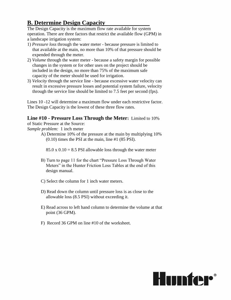
Line #10 - Pressure Loss Through the Meter: Limited to 10%
of Static Pressure at the Source:
Sample problem: 1 inch meter
A) Determine 10% of the pressure at the main by multiplying 10%
(0.10) times the PSI at the main, line #1 (85 PSI).
85.0 x 0.10 = 8.5 PSI allowable loss through the water meter
B) Turn to page 11 for the chart “Pressure Loss Through Water
Meters” in the Hunter Friction Loss Tables at the end of this
design manual.
C) Select the column for 1 inch water meters.
D) Read down the column until pressure loss is as close to the
allowable loss (8.5 PSI) without exceeding it.
E) Read across to left hand column to determine the volume at that
point (36 GPM).
F) Record 36 GPM on line #10 of the worksheet.
Line #11 - Volume Through the Meter: Limited to 75% of Water
Meter Capacity
Sample problem: 1 inch water meter
A) Turn to page 11 for the chart “Pressure Loss Through Water
Meters” in the Hunter Friction Loss Tables at the end of this
design manual.
B) Locate the column for size of water meter (1 inch).
C) Read down the pressure loss column under 1 inch meters until
pressure loss figures stop.
D) Read across to left hand column to determine the volume at that
point (50 GPM). This represents the maximum safe flow for that
size meter.
E) Determine 75% of maximum safe flow by multiplying the flow
by 75% (0.75).
50 GPM x 0.75 = 37.5 GPM
F) Record 37.5 GPM on line #11 of the worksheet.
Line #12 - Velocity in the Service Line: This is the friction loss
due to the speed at which water flows through the service line. Because
excessive water velocity can result in excessive pressure losses and
potential system failure, velocity through the service line is limited to 7.5
Feet Per Second (fps)*.
Sample Problem: 1-1/4 inch Type “K” Copper
A) Turn to the chart for the type of service line used, page 9 in the
Hunter Friction Loss Tables at the end of this design manual.
B) Locate the column for the size of service line (1-1/4 inch).
C) Read down the column for velocity (fps) until the velocity
reaches 7.5 fps (or as high a velocity as listed without exceeding
7.5 fps).
D) Read across from that point to the left hand column to
determine volume (GPM) at allowed 7.5 fps (28 GPM).
E) Record 28 GPM on line #12 of the worksheet.

Note: This 7-1/2 fps restriction is sometimes disregarded in the industry
because service line is usually copper and is unlikely to be damaged by
water hammer. If you disregard this restriction, a check of actual
pressure loss through the service line must be made to insure the
pressure loss incurred due to high velocity is not excessive. Conversely,
some areas will not allow a velocity as high as 7-1/2 fps -- check the
local restrictions.
Line #13 - Design Capacity: Lowest of the three flow rates listed on
Lines 10 - 12. The lowest flow rate is selected because this flow rate is the
only one that will not exceed any of the three restrictions on Design
Capacity: Pressure Loss Through the Meter, Volume Through the Meter,
and Velocity Through the Service Line. List the lowest of the three flow
rates on line #13.
Sample Problem: 28 GPM
C. Calculate Dynamic Pressure at Design Capacity Now that a flow rate (Design Capacity) has been established, this flow rate
can be used to estimate the dynamic pressure at the Point of Connection.
Pressure losses from the source to the POC include those through the
service line, delivery line, water meter, isolation valves, or other system
components. Note: not all components listed are present in all systems.
Line #14 - Pressure Loss in the Service Line: Determine the
pressure loss in the service line.
Sample Problem: 1-1/4 inch Type “K” Copper
A) Turn to the chart for the type of service line used, page 9 in the
Hunter Friction Loss Tables at the end of this design manual.
B) Read down the left hand column (Flow GPM) to the design
capacity, line #13.
Sample Problem: 28 GPM
C) Read across to the right from that point to the column for PSI
loss in 1-1/4” “K” copper.
Sample Problem: 7.97 PSI per 100 ft.
D) Record this in the first space on line #14.
Sample Problem: 7.97
E) Record the length of the service line in the second space on line
#14, this information was recorded on line #5 of the worksheet.
Sample Problem: 25 ft.
F) Determine the pressure loss through the service line by
multiplying the pressure loss per 100 ft. times the length of the
service line and dividing the answer by 100 to find the actual
PSI loss in the service line.
Sample Problem:
(7.97 x 25) = 1.99 PSI loss in the service line
100
G) Record this PSI loss on line #14 of the worksheet.
Sample Problem: 1.99
Line #15 - Pressure Loss in the Delivery Line: Determine the
pressure loss in the delivery line.
Sample Problem: Schedule 40 PVC
A) Turn to the chart for the type of delivery line used, page 2 in the
Hunter Friction Loss Tables at the end of this design manual.
B) Read down the left hand column (Flow GPM) to the design
capacity, line #13.
Sample Problem: 28 GPM
C) Read across to the right from that point to the column for PSI
loss in 1-1/4” Schedule 40 PVC.
Sample Problem: 4.25 PSI per 100 ft.
D) Record this in the first space on line #15.
Sample Problem: 4.25
E) Record the length of the delivery line in the second space on
line #15. This information was recorded on line #6 of the
worksheet.
Sample Problem: 65
F) Determine the pressure loss through the delivery line by
multiplying the pressure loss per 100 ft. times the length of the
delivery line and dividing the answer by 100 to find the actual
PSI loss in the delivery line.
Sample Problem:
(4.25 x 65) = 2.76 PSI loss in the service line
100
G) Record this PSI loss on line #15 of the worksheet.
Sample Problem: 2.76
Line #16 - Pressure Loss in the Water Meter: Determine the
pressure loss in the water meter.
A) Turn to page 11 for the chart “Pressure Loss Through Water
Meters” in the Hunter Friction Loss Tables at the end of this
design manual.
B) Read down the left hand column (Flow GPM) to the design
capacity, line #13.
Sample Problem: 28 GPM
C) Read across to the right from that point to the column for
pressure loss in 1 inch water meters.
Sample Problem: 4.60 PSI loss
D) Record this PSI loss on line #16 of the worksheet.
Sample Problem: 4.60
Line #17 - Pressure Loss in the Isolation Valves: Isolation
valves may be gate valves, ball valves, globe valves, meter cocks or curb
stops. While there will be a meter cock or curb stop in most municipal
systems, the pressure losses incurred are generally considered minimal. If
they are included, pressure losses can be estimated by use of the
equivalent length chart, “Pressure Loss in Valves and Fittings,” on page
10 in the Hunter Friction Loss Tables at the end of this design manual.
There are no isolation valves included in this example.
Line #18 - Other Pressure Losses: These may include pressure
losses through backflow prevention devices, filters or other system
components located between the water source and the POC.
Manufacturers publish pressure loss (also known as friction loss)
information in their product catalogs. There are no other components for
this example.
Line #19 - Pressure Loss from the Source to POC: Add the
pressure losses recorded on lines 14 - 18.
Sample Problem: 1.99 + 2.76 + 4.60 + 0.0 + 0.0 = 9.35 PSI

Line #20 - Approximate Dynamic Pressure at Design
Capacity:
1) Record the static pressure previously determined on line #4.
2) Record the pressure loss subtotal from line #19.
3) Subtract these two lines to determine the approximate dynamic
pressure expected at the POC at the maximum system flow rate
(Design Capacity).
Sample Problem:
static pressure from line #4 77.64 PSI
pressure loss subtotal from line #19 - 9.35 PSI
approximate Dynamic Pressure at the POC 68.29 PSI
D. Estimate Pressure Available at
"Worst Case" Head At this point the Design Capacity (GPM from line #13) and Dynamic
Pressure at the POC (PSI from line #20) have been calculated. The Design
Capacity establishes the maximum flow rate for the system and the
Dynamic Pressure at the POC provides us with a basis for estimating the
dynamic pressure that will be available to operate the sprinklers.
In order to begin our irrigation system design, an estimate of the available
dynamic pressure at the worst case head must be made. This is calculated
by:
1) Adding or subtracting the pressure change due to the change in
elevation between the POC and the highest head in the system.
2) Estimating the amount of pressure that would remain after normal
pressure losses between the POC and the highest head; typically 1/3 of
the available dynamic pressure is lost and 2/3 remains available for
sprinkler operation.

Line #21 - Pressure Change Due to Elevation Change:
Calculate the pressure change due to elevation between the POC and the
highest head.
Sample Problem: the highest head is 10 ft. above the POC. 10 x
0.433 = 4.33 PSI
Line #22 - Estimated Pressure Subtotal: If the highest head in
the system is above the POC, subtract the pressure change calculated on
line #21 from line #20, if the highest head is lower than the POC, the
pressure change from line #21 must be added to the pressure on line #20.
Sample Problem: 68.29 - 4.33 = 63.96 PSI
Line #23 - Two Thirds Estimate: A normal landscape irrigation
system will lose approximately one third (1/3) of the dynamic pressure
available between the POC and the highest head. These losses occur
because of friction loss in pipe, pressure loss in valves and fittings, and
pressure loss through backflow prevention devices or other system
components. Because of these losses, only two thirds of the dynamic
pressure available at the POC is available for sprinkler operation. In this
step, multiply the pressure subtotal calculated on line #22 by 2/3 (0.67).
Sample Problem: 63.96 x 0.67 = 42.85 PSI

How To Use The Worksheet Information With this worksheet you have determined the following:
• Design Capacity (line #13): The Design Capacity is the maximum safe
flow available for use in the sprinkler system. This flow will determine
how many heads can be operated at any one time. For example, if the
design capacity is 18 GPM, the system can have six 3 GPM heads
operating at one time (6 heads x 3 GPM = 18 GPM). If more than 6 heads
are needed for the project, additional valves must be added so that no more
than 18 GPM would be used at one time.
• Dynamic Pressure at Design Capacity (line #20): This is the dynamic
pressure that can be expected at the POC when the system is using the
maximum safe flow (Design Capacity, line #13). This figure is used 1) as
a starting point in estimating the pressure that will be available at the
worst case head, and 2) as a guideline when the irrigation design is
completed to check total system pressure required and assure the system is
designed correctly.
• Estimated Pressure Available for Sprinkler Operation (line #23):
This is an estimate of the dynamic pressure available for sprinkler
operation at the highest head in the system. If there is a significant drop in
elevation to the location of other heads in the system, the pressure gain due
to the drop in elevation could be added to this figure. This pressure should
be used as a guide for selecting sprinklers. For example, if the pressure on
line #23 is 40 PSI, then sprinklers selected for the project should have
operating pressures of 40 PSI or less.
After the preliminary design has been completed, a thorough calculation
of the friction loss in the system should be made before committing to the
final irrigation plan. This calculation should include friction loss in the
lateral lines and all other components back to the point of connection, and
should be based on the GPM actually expected to be used by the sprinkler
heads chosen. This subject is covered later under “Friction Losses”.

Design Problem Many times, you will use a pressure gauge attached to an outside faucet to
measure the static pressure. When measuring the PSI in this manner, be
sure that no water is running anywhere on the property. Be aware that the
static pressure can vary throughout the day; it’s best to take the pressure
measurement at the same time of day as you plan on watering.
Remember: the static pressure at the POC will be greater if the
measurement is taken at a point above the POC, and lower at the POC if
the measurement is taken at a point below the POC.
Using the following design and the information below, complete a Design
Capacity and Working Pressure worksheet :
Static Pressure at P.O.C. 72 PSI
Net elevation change - P.O.C. to highest head +3 ft.
Service Line 15 ft. 1-1/4” Type K Copper
Delivery Line 5 ft. 1” Type K Copper
Water Meter size 5/8”
70 psi
Measured
3 ft. - POC to
Highest Head 5 ft. to POC
Sprinkler
System POC
1 in. Type “K” Copper
Delivery Line - 5 ft.
1-1/4 in Type “K” Copper
Service Line - 15 ft.
City Water Main
Static Pressure at POC is measured as follows:
1. Static pressure measured at the hose bib is 70 psi.
2. Elevation change from the hose bib to the POC is 5 feet (POC is lower).
3. 5 ft x .433 psi/ft = 2.165 psi
4. 70 psi + 2.165 psi = 72.165 psi at the POC
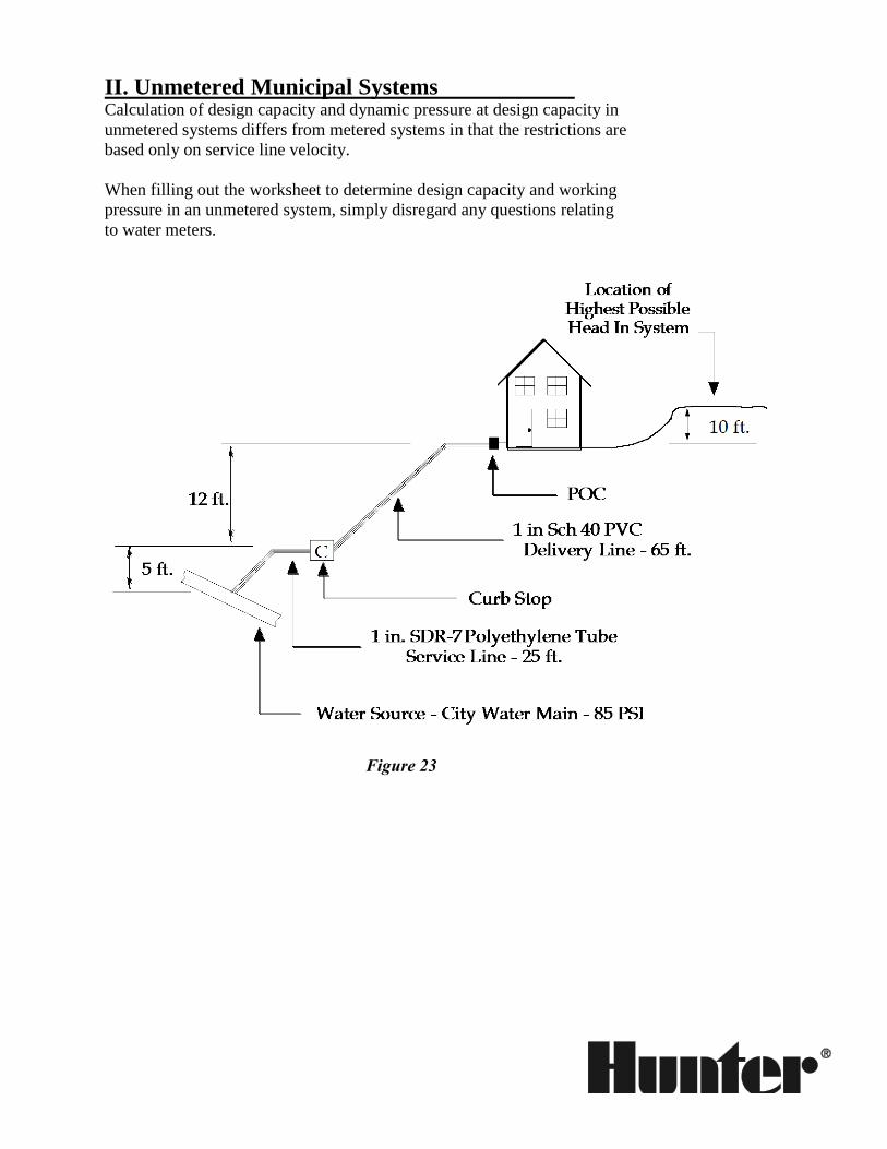
II. Unmetered Municipal Systems Calculation of design capacity and dynamic pressure at design capacity in
unmetered systems differs from metered systems in that the restrictions are
based only on service line velocity.
When filling out the worksheet to determine design capacity and working
pressure in an unmetered system, simply disregard any questions relating
to water meters.
Figure 23
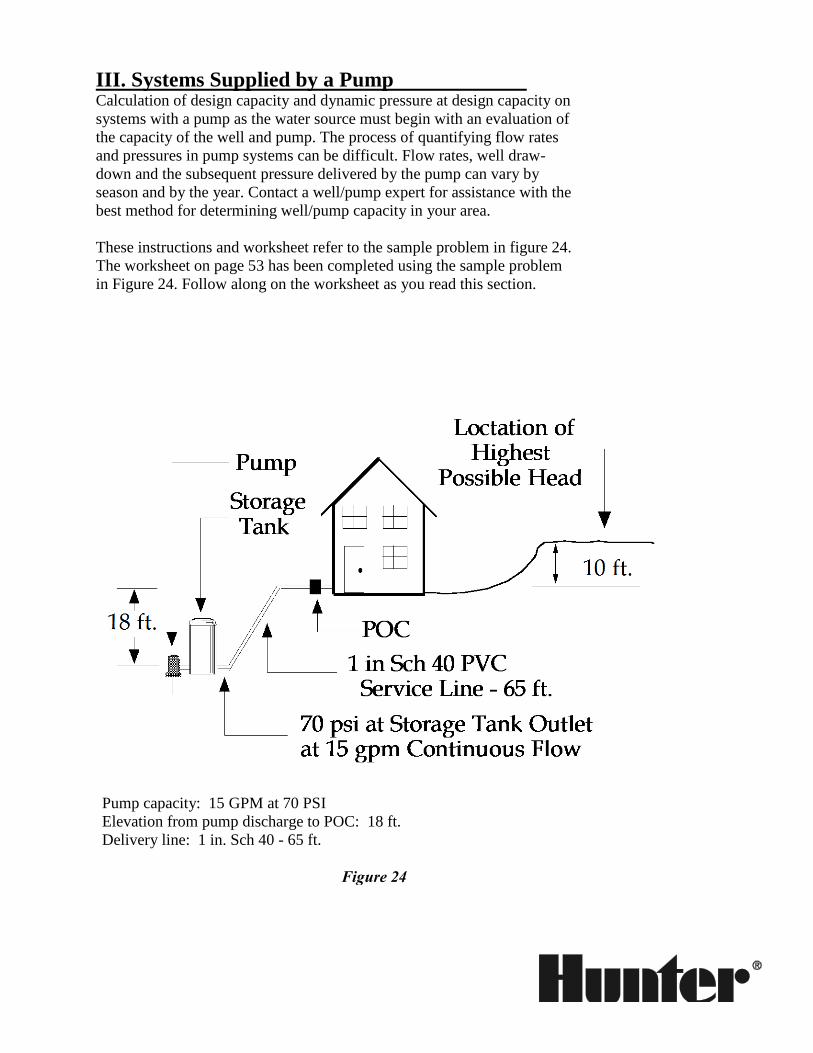
III. Systems Supplied by a Pump Calculation of design capacity and dynamic pressure at design capacity on
systems with a pump as the water source must begin with an evaluation of
the capacity of the well and pump. The process of quantifying flow rates
and pressures in pump systems can be difficult. Flow rates, well draw-
down and the subsequent pressure delivered by the pump can vary by
season and by the year. Contact a well/pump expert for assistance with the
best method for determining well/pump capacity in your area.
These instructions and worksheet refer to the sample problem in figure 24.
The worksheet on page 53 has been completed using the sample problem
in Figure 24. Follow along on the worksheet as you read this section.
Pump capacity: 15 GPM at 70 PSI
Elevation from pump discharge to POC: 18 ft.
Delivery line: 1 in. Sch 40 - 65 ft.
Figure 24
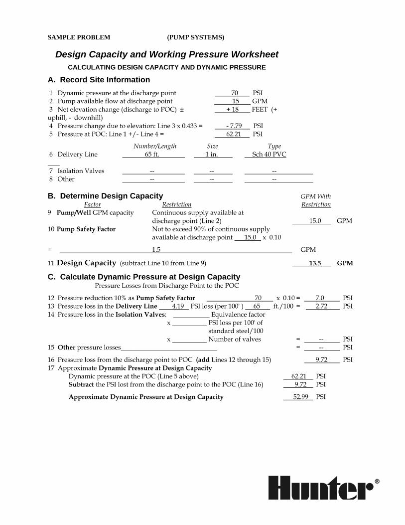
SAMPLE PROBLEM (PUMP SYSTEMS)
Design Capacity and Working Pressure Worksheet
CALCULATING DESIGN CAPACITY AND DYNAMIC PRESSURE
A. Record Site Information
1 Dynamic pressure at the discharge point 70 PSI 2 Pump available flow at discharge point 15 GPM 3 Net elevation change (discharge to POC) ± + 18 FEET (+ uphill, - downhill) 4 Pressure change due to elevation: Line 3 x 0.433 = - 7.79 PSI 5 Pressure at POC: Line 1 +/- Line 4 = 62.21 PSI
Number/Length Size Type 6 Delivery Line 65 ft. 1 in. Sch 40 PVC 7 Isolation Valves -- -- -- 8 Other -- -- --
B. Determine Design Capacity GPM With Factor Restriction Restriction 9 Pump/Well GPM capacity Continuous supply available at discharge point (Line 2) 15.0 GPM 10 Pump Safety Factor Not to exceed 90% of continuous supply available at discharge point 15.0 x 0.10
= 1.5 GPM
11 Design Capacity (subtract Line 10 from Line 9) 13.5 GPM
C. Calculate Dynamic Pressure at Design Capacity Pressure Losses from Discharge Point to the POC
12 Pressure reduction 10% as Pump Safety Factor 70 x 0.10 = 7.0 PSI 13 Pressure loss in the Delivery Line 4.19 PSI loss (per 100' ) 65 ft./100 = 2.72 PSI 14 Pressure loss in the Isolation Valves: Equivalence factor x PSI loss per 100' of standard steel/100 x Number of valves = -- PSI 15 Other pressure losses_____________________________ = -- . PSI
16 Pressure loss from the discharge point to POC (add Lines 12 through 15) 9.72 PSI 17 Approximate Dynamic Pressure at Design Capacity Dynamic pressure at the POC (Line 5 above) 62.21 PSI Subtract the PSI lost from the discharge point to the POC (Line 16) 9.72 PSI
Approximate Dynamic Pressure at Design Capacity 52.99 PSI

D. Estimate Pressure Available at “Worst-Case” Head
18 Pressure change due to elevation change from the POC to the highest head in the system. 10 ft. x 0.433 = 4.33 PSI 19 Pressure subtotal (subtract Line 18 from Line 17; for worst case heads which are lower than the POC, add Lines 17 and 18) 48.66 PSI 20 Estimated Pressure Available at worst case-head two-thirds of subtotal: Line 19 48.66 PSI x 0.67 = 32.60 PSI
Pressure Available for Sprinkler Selection and Operation 32.60 PSI

A. Record Site Information Line #1 - Dynamic Pressure at the Discharge Point: The
pressure and the design capacity of pump/well systems differ from
municipal systems in that they are dependent on the capacity of individual
pumps and wells. These flow rates and pressures vary widely even
between wells located close to one another. Well/pump systems differ in
the determination of design capacity because of the need to establish the
capacity of the well or pump. This flow can vary from just a few gallons
per minute to hundreds of gallons per minute. The pump/well capacity and
the pump's discharge pressure may be obtained from:
1) The property owner - if they have records from past pump/well
tests.
2) The company installing the pump.
3) An on-site test conducted by a pump engineer or well drilling
firm.
Sample Problem: Dynamic pressure at the discharge point = 70 PSI
Line #2 - Available Flow at the Discharge Point: This is
obtainable from the above sources. (With pump systems, available flow is
generally stated as "___ GPM at ___ PSI".)
Sample Problem: 15 GPM
Line #3 - Net Elevation Change: The net elevation change is
determined by estimating the difference in elevation from the discharge
point of the pump or well (point used on line #1) to the sprinkler system
POC.
Sample Problem: Elevation gain = 18’
Line #4 - Pressure Change Due to Elevation: This is calculated
by multiplying the elevation change from the discharge point to the POC
(line #3) by 0.433 PSI (PSI change per foot of elevation change).
Sample Problem: 18’ x 0.433 PSI per ft. = 7.79 PSI
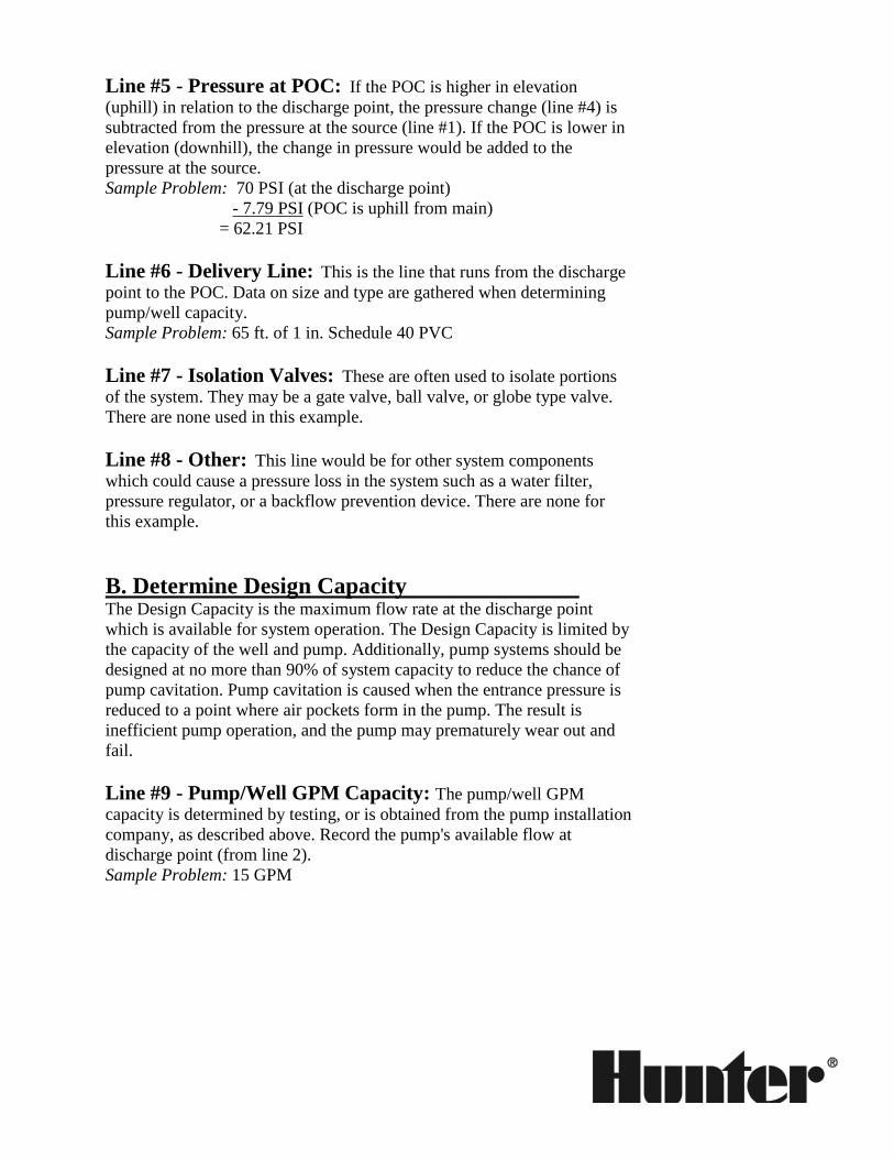
Line #5 - Pressure at POC: If the POC is higher in elevation
(uphill) in relation to the discharge point, the pressure change (line #4) is
subtracted from the pressure at the source (line #1). If the POC is lower in
elevation (downhill), the change in pressure would be added to the
pressure at the source.
Sample Problem: 70 PSI (at the discharge point)
- 7.79 PSI (POC is uphill from main)
= 62.21 PSI
Line #6 - Delivery Line: This is the line that runs from the discharge
point to the POC. Data on size and type are gathered when determining
pump/well capacity.
Sample Problem: 65 ft. of 1 in. Schedule 40 PVC
Line #7 - Isolation Valves: These are often used to isolate portions
of the system. They may be a gate valve, ball valve, or globe type valve.
There are none used in this example.
Line #8 - Other: This line would be for other system components
which could cause a pressure loss in the system such as a water filter,
pressure regulator, or a backflow prevention device. There are none for
this example.
B. Determine Design Capacity The Design Capacity is the maximum flow rate at the discharge point
which is available for system operation. The Design Capacity is limited by
the capacity of the well and pump. Additionally, pump systems should be
designed at no more than 90% of system capacity to reduce the chance of
pump cavitation. Pump cavitation is caused when the entrance pressure is
reduced to a point where air pockets form in the pump. The result is
inefficient pump operation, and the pump may prematurely wear out and
fail.
Line #9 - Pump/Well GPM Capacity: The pump/well GPM
capacity is determined by testing, or is obtained from the pump installation
company, as described above. Record the pump's available flow at
discharge point (from line 2).
Sample Problem: 15 GPM
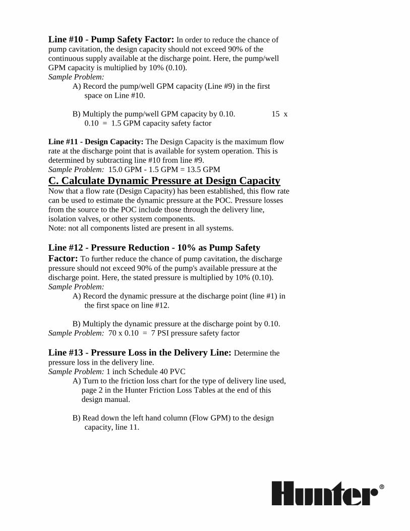
Line #10 - Pump Safety Factor: In order to reduce the chance of
pump cavitation, the design capacity should not exceed 90% of the
continuous supply available at the discharge point. Here, the pump/well
GPM capacity is multiplied by 10% (0.10).
Sample Problem:
A) Record the pump/well GPM capacity (Line #9) in the first
space on Line #10.
B) Multiply the pump/well GPM capacity by 0.10. 15 x
0.10 = 1.5 GPM capacity safety factor
Line #11 - Design Capacity: The Design Capacity is the maximum flow
rate at the discharge point that is available for system operation. This is
determined by subtracting line #10 from line #9.
Sample Problem: 15.0 GPM - 1.5 GPM = 13.5 GPM
C. Calculate Dynamic Pressure at Design Capacity Now that a flow rate (Design Capacity) has been established, this flow rate
can be used to estimate the dynamic pressure at the POC. Pressure losses
from the source to the POC include those through the delivery line,
isolation valves, or other system components.
Note: not all components listed are present in all systems.
Line #12 - Pressure Reduction - 10% as Pump Safety
Factor: To further reduce the chance of pump cavitation, the discharge
pressure should not exceed 90% of the pump's available pressure at the
discharge point. Here, the stated pressure is multiplied by 10% (0.10).
Sample Problem:
A) Record the dynamic pressure at the discharge point (line #1) in
the first space on line #12.
B) Multiply the dynamic pressure at the discharge point by 0.10.
Sample Problem: 70 x 0.10 = 7 PSI pressure safety factor
Line #13 - Pressure Loss in the Delivery Line: Determine the
pressure loss in the delivery line.
Sample Problem: 1 inch Schedule 40 PVC
A) Turn to the friction loss chart for the type of delivery line used,
page 2 in the Hunter Friction Loss Tables at the end of this
design manual.
B) Read down the left hand column (Flow GPM) to the design
capacity, line 11.
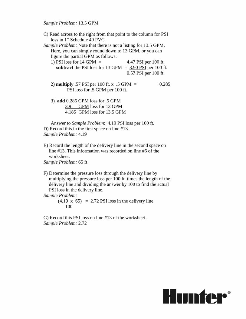
Sample Problem: 13.5 GPM
C) Read across to the right from that point to the column for PSI
loss in 1” Schedule 40 PVC.
Sample Problem: Note that there is not a listing for 13.5 GPM.
Here, you can simply round down to 13 GPM, or you can
figure the partial GPM as follows:
1) PSI loss for 14 GPM = 4.47 PSI per 100 ft.
subtract the PSI loss for 13 GPM = 3.90 PSI per 100 ft.
0.57 PSI per 100 ft.
2) multiply .57 PSI per 100 ft. x .5 GPM = 0.285
PSI loss for .5 GPM per 100 ft.
3) add 0.285 GPM loss for .5 GPM
3.9 GPM loss for 13 GPM
4.185 GPM loss for 13.5 GPM
Answer to Sample Problem: 4.19 PSI loss per 100 ft.
D) Record this in the first space on line #13.
Sample Problem: 4.19
E) Record the length of the delivery line in the second space on
line #13. This information was recorded on line #6 of the
worksheet.
Sample Problem: 65 ft
F) Determine the pressure loss through the delivery line by
multiplying the pressure loss per 100 ft. times the length of the
delivery line and dividing the answer by 100 to find the actual
PSI loss in the delivery line.
Sample Problem:
(4.19 x 65) = 2.72 PSI loss in the delivery line
100
G) Record this PSI loss on line #13 of the worksheet.
Sample Problem: 2.72

Line #14 - Pressure Loss in the Isolation Valves: Isolation
valves may be gate valves, ball valves, or globe valves. While there will
be a meter cock or curb stop in most municipal systems, the pressure
losses incurred are generally considered minimal. If they are included,
pressure losses can be estimated by use of the equivalent length chart,
“Pressure Loss in Valves and Fittings,” on page 10 in the Hunter Friction
Loss Tables at the end of this design manual.
There are no isolation valves in this example.
Line #15 - Other Pressure Losses: These may include pressure
losses through backflow prevention devices, filters, or other system
components located between the water source and the POC. There are
none in this example.
Line #16 - Pressure Loss from the Source to POC: Add the
pressure losses recorded on lines 12 - 15.
Sample Problem: 7.0 + 2.72 + 0.0 + 0.0 = 9.72 PSI
Line #17 - Approximate Dynamic Pressure at Design
Capacity:
1) Record the pressure previously determined on line #5.
2) Record the pressure loss subtotal from line #16.
3) Subtract these two lines to determine the approximate dynamic
pressure expected at the POC at the maximum system flow rate
(Design Capacity).
Sample Problem:
pressure from line #5 62.21 PSI
pressure loss subtotal from line #16 - 9.72 PSI
approximate Dynamic Pressure at the POC 52.99 PSI

D. Estimate Pressure Available at
"Worst Case" Head At this point the Design Capacity (GPM from line #11) and Dynamic
Pressure at the POC have been calculated. The Design Capacity
establishes the maximum flow rate for the system and the Dynamic
Pressure at the POC provides us with a basis for estimating the dynamic
pressure that will be available to operate the sprinklers.
In order to begin our irrigation system design an estimate of the available
dynamic pressure at the worst case head must be made. This is calculated
by:
1) Adding or subtracting the pressure change due to the change in
elevation between the POC and the highest head in the system.
2) Estimating the amount of pressure that would remain after normal
pressure losses between the POC and the highest head; typically 1/3 of
the available dynamic pressure is lost and 2/3 remains available for
sprinkler operation
Line #18 - Pressure Change Due to Elevation Change:
Calculate the pressure change due to elevation between the POC and the
highest head.
Sample Problem: the highest head is 10 ft. above the POC.
10 x 0.433 = 4.33 PSI
Line #19 - Estimated Pressure Available for Sprinkler
Operation: If the highest head in the system is above the POC, subtract
the pressure change calculated on line #18 from line #17, if the highest
head is lower than the POC, the pressure change from line #18 must be
added to the pressure on line #17.
Sample Problem: 52.99 - 4.33 = 48.66 PSI
Line #20 - Two Thirds Estimate: A normal landscape irrigation
system will lose approximately one third (1/3) of the dynamic pressure
available between the POC and the highest head. These losses occur
because of friction loss in pipe, pressure loss in valves and fittings, and
pressure loss through check valves or other system components. Because
of these losses, only two thirds of the dynamic pressure available at the
POC is available for sprinkler operation. In this step, multiply the pressure
subtotal calculated on line #19 by 2/3 (0.67).
Sample Problem: 48.66 x 0.67 = 32.60 PSI
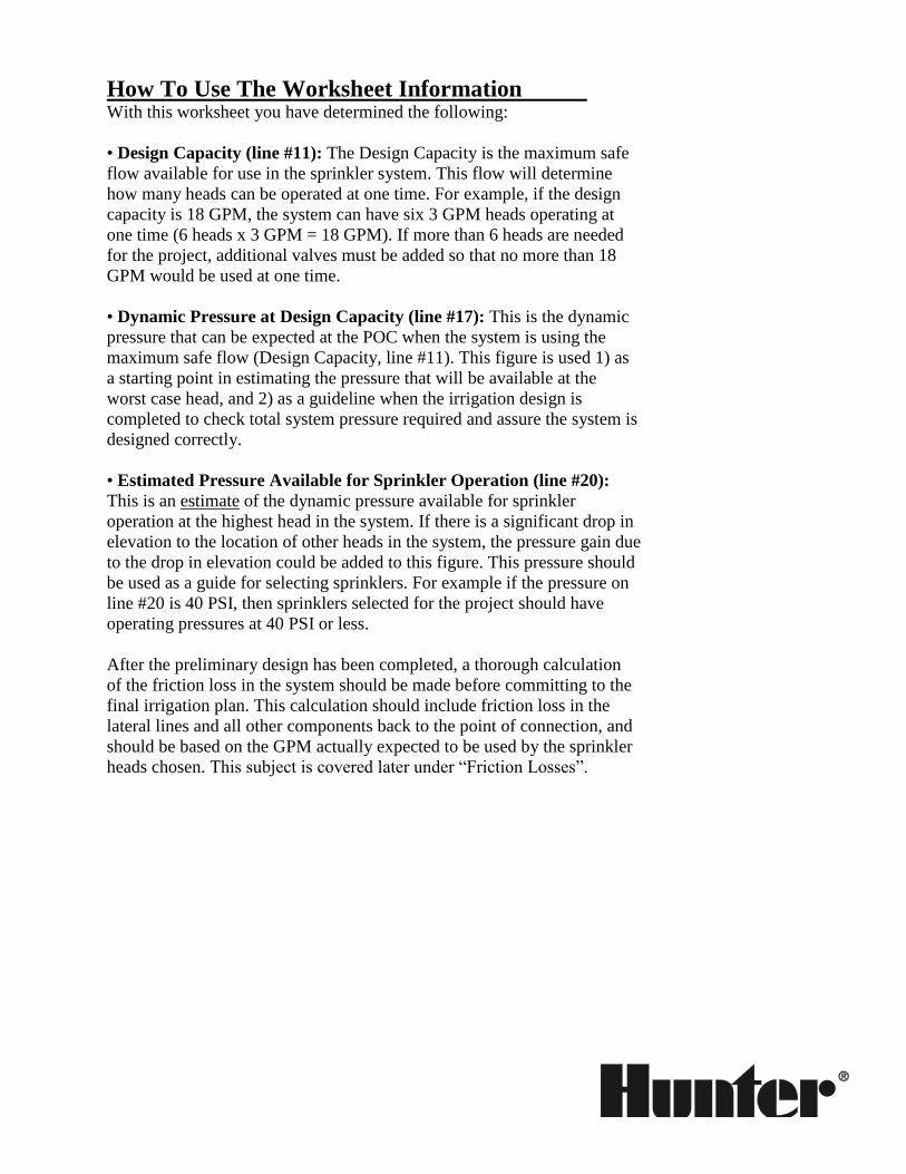
How To Use The Worksheet Information With this worksheet you have determined the following:
• Design Capacity (line #11): The Design Capacity is the maximum safe
flow available for use in the sprinkler system. This flow will determine
how many heads can be operated at one time. For example, if the design
capacity is 18 GPM, the system can have six 3 GPM heads operating at
one time (6 heads x 3 GPM = 18 GPM). If more than 6 heads are needed
for the project, additional valves must be added so that no more than 18
GPM would be used at one time.
• Dynamic Pressure at Design Capacity (line #17): This is the dynamic
pressure that can be expected at the POC when the system is using the
maximum safe flow (Design Capacity, line #11). This figure is used 1) as
a starting point in estimating the pressure that will be available at the
worst case head, and 2) as a guideline when the irrigation design is
completed to check total system pressure required and assure the system is
designed correctly.
• Estimated Pressure Available for Sprinkler Operation (line #20):
This is an estimate of the dynamic pressure available for sprinkler
operation at the highest head in the system. If there is a significant drop in
elevation to the location of other heads in the system, the pressure gain due
to the drop in elevation could be added to this figure. This pressure should
be used as a guide for selecting sprinklers. For example if the pressure on
line #20 is 40 PSI, then sprinklers selected for the project should have
operating pressures at 40 PSI or less.
After the preliminary design has been completed, a thorough calculation
of the friction loss in the system should be made before committing to the
final irrigation plan. This calculation should include friction loss in the
lateral lines and all other components back to the point of connection, and
should be based on the GPM actually expected to be used by the sprinkler
heads chosen. This subject is covered later under “Friction Losses”.

(METERED SYSTEMS)
Design Capacity and Working Pressure Worksheet
CALCULATING DESIGN CAPACITY AND DYNAMIC PRESSURE
A. Record Site Information
1 Static* Pressure at the Source (Main) PSI 2 Net elevation Change (Source to POC) ± FEET (+ uphill, - downhill) 3 Pressure change due to elevation: Line 2 x 0.433 = PSI 4 Static Pressure at POC: Line 1 +/- Line 3 = PSI Number/Length Size Type 5 Service Line 6 Delivery Line 7 Water Meter 8 Isolation Valves 9 Other
B. Determine Design Capacity GPM With Factor Restriction Restriction 10 Pressure loss through Not to exceed 10% of available the water meter. PSI at the source(Line 1) GPM 11 Volume through the Not to exceed 75% of maximum water meter. safe flow of the meter. GPM 12 Velocity through the Velocity not to exceed 7.5 fps service line. (Main to meter) GPM
13 Design Capacity Lowest GPM of the three flows rates - lines 10, 11, and 12. GPM
C. Calculate Dynamic Pressure at Design Capacity Pressure Losses from Source(City Water Main) to the POC
14 Pressure loss in the Service Line PSI loss (per 100' ) x ft./100 = PSI 15 Pressure loss in the Delivery Line PSI loss (per 100' ) x ft./100 = PSI 16 Pressure loss in the Water Meter at design capacity = PSI 17 Pressure loss in the Gate Valves: _____ Equivalence Factor x _____ PSI loss per 100' of Standard Steel/100 x _____ Number of Gate Valves = PSI 18 Other pressure losses_____________________________ = PSI 19 Pressure loss from the source to POC (add Lines 14 through 18) PSI 20 Approximate Dynamic Pressure at Design Capacity Static Pressure at the POC (Line 4 above) PSI Subtract the PSI lost from the source to the POC (Line 19 ) PSI Approximate Dynamic Pressure at Design Capacity PSI

D. Estimate Pressure Available at “Worst-Case” Head
21 Pressure change due to elevation change from the POC to the highest head in the system. ft. x 0.433 = PSI 22 Pressure subtotal (subtract Line 21 from Line 20; for worst case heads which are lower than the POC, add Lines 20 and 21) PSI 23 Estimated Pressure Available at worst case-head two-thirds of subtotal: Line 22 PSI x 0.67 = PSI
Pressure Available for Sprinkler Selection and Operation PSI
*Although this is referred to as static pressure, in municipal systems it is taken to mean the minimum
dynamic pressure at the water main.
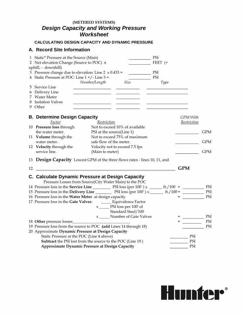
(METERED SYSTEMS)
Design Capacity and Working Pressure Worksheet
CALCULATING DESIGN CAPACITY AND DYNAMIC PRESSURE
A. Record Site Information
1 Static* Pressure at the Source (Main) PSI 2 Net elevation Change (Source to POC) ± FEET (+ uphill, - downhill) 3 Pressure change due to elevation: Line 2 x 0.433 = PSI 4 Static Pressure at POC: Line 1 +/- Line 3 = PSI Number/Length Size Type 5 Service Line 6 Delivery Line 7 Water Meter 8 Isolation Valves 9 Other
B. Determine Design Capacity GPM With Factor Restriction Restriction 10 Pressure loss through Not to exceed 10% of available the water meter. PSI at the source(Line 1) GPM 11 Volume through the Not to exceed 75% of maximum water meter. safe flow of the meter. GPM 12 Velocity through the Velocity not to exceed 7.5 fps service line. (Main to meter) GPM
13 Design Capacity Lowest GPM of the three flows rates - lines 10, 11, and
12. GPM
C. Calculate Dynamic Pressure at Design Capacity Pressure Losses from Source(City Water Main) to the POC
14 Pressure loss in the Service Line PSI loss (per 100' ) x ft./100 = PSI 15 Pressure loss in the Delivery Line PSI loss (per 100' ) x ft./100 = PSI 16 Pressure loss in the Water Meter at design capacity = PSI 17 Pressure loss in the Gate Valves: _____ Equivalence Factor x _____ PSI loss per 100' of Standard Steel/100 x _____ Number of Gate Valves = PSI 18 Other pressure losses_____________________________ = PSI 19 Pressure loss from the source to POC (add Lines 14 through 18) PSI 20 Approximate Dynamic Pressure at Design Capacity Static Pressure at the POC (Line 4 above) PSI Subtract the PSI lost from the source to the POC (Line 19 ) PSI Approximate Dynamic Pressure at Design Capacity PSI

D. Estimate Pressure Available at “Worst-Case” Head
21 Pressure change due to elevation change from the POC to the highest head in the system. ft. x 0.433 = PSI 22 Pressure subtotal (subtract Line 21 from Line 20; for worst case heads which are lower than the POC, add Lines 20 and 21) PSI 23 Estimated Pressure Available at worst case-head two-thirds of subtotal: Line 22 PSI x 0.67 = PSI
Pressure Available for Sprinkler Selection and Operation PSI
*Although this is referred to as static pressure, in municipal systems it is taken to mean the minimum dynamic pressure at the water main

(METERED SYSTEMS)
Design Capacity and Working Pressure Worksheet
CALCULATING DESIGN CAPACITY AND DYNAMIC PRESSURE
A. Record Site Information
1 Static* Pressure at the Source (Main) PSI 2 Net elevation Change (Source to POC) ± FEET (+ uphill, - downhill) 3 Pressure change due to elevation: Line 2 x 0.433 = PSI 4 Static Pressure at POC: Line 1 +/- Line 3 = PSI Number/Length Size Type 5 Service Line 6 Delivery Line 7 Water Meter 8 Isolation Valves 9 Other
B. Determine Design Capacity GPM With Factor Restriction Restriction 10 Pressure loss through Not to exceed 10% of available the water meter. PSI at the source(Line 1) GPM 11 Volume through the Not to exceed 75% of maximum water meter. safe flow of the meter. GPM 12 Velocity through the Velocity not to exceed 7.5 fps service line. (Main to meter) GPM
13 Design Capacity Lowest GPM of the three flows rates - lines 10, 11, and
12. GPM
C. Calculate Dynamic Pressure at Design Capacity Pressure Losses from Source(City Water Main) to the POC
14 Pressure loss in the Service Line PSI loss (per 100' ) x ft./100 = PSI 15 Pressure loss in the Delivery Line PSI loss (per 100' ) x ft./100 = PSI 16 Pressure loss in the Water Meter at design capacity = PSI 17 Pressure loss in the Gate Valves: _____ Equivalence Factor x _____ PSI loss per 100' of Standard Steel/100 x _____ Number of Gate Valves = PSI 18 Other pressure losses_____________________________ = PSI 19 Pressure loss from the source to POC (add Lines 14 through 18) PSI 20 Approximate Dynamic Pressure at Design Capacity Static Pressure at the POC (Line 4 above) PSI Subtract the PSI lost from the source to the POC (Line 19 ) PSI Approximate Dynamic Pressure at Design Capacity PSI

D. Estimate Pressure Available at “Worst-Case” Head
21 Pressure change due to elevation change from the POC to the highest head in the system. ft. x 0.433 = PSI 22 Pressure subtotal (subtract Line 21 from Line 20; for worst case heads which are lower than the POC, add Lines 20 and 21) PSI 23 Estimated Pressure Available at worst case-head two-thirds of subtotal: Line 22 PSI x 0.67 = PSI
Pressure Available for Sprinkler Selection and Operation PSI
*Although this is referred to as static pressure, in municipal systems it is taken to mean the minimum
dynamic pressure at the water main.

(METERED SYSTEMS)
Design Capacity and Working Pressure Worksheet
CALCULATING DESIGN CAPACITY AND DYNAMIC PRESSURE
A. Record Site Information
1 Static* Pressure at the Source (Main) PSI 2 Net elevation Change (Source to POC) ± FEET (+ uphill, - downhill) 3 Pressure change due to elevation: Line 2 x 0.433 = PSI 4 Static Pressure at POC: Line 1 +/- Line 3 = PSI Number/Length Size Type 5 Service Line 6 Delivery Line 7 Water Meter 8 Isolation Valves 9 Other
B. Determine Design Capacity GPM With Factor Restriction Restriction 10 Pressure loss through Not to exceed 10% of available the water meter. PSI at the source(Line 1) GPM 11 Volume through the Not to exceed 75% of maximum water meter. safe flow of the meter. GPM 12 Velocity through the Velocity not to exceed 7.5 fps service line. (Main to meter) GPM
13 Design Capacity Lowest GPM of the three flows rates - lines 10, 11, and
12. GPM
C. Calculate Dynamic Pressure at Design Capacity Pressure Losses from Source(City Water Main) to the POC
14 Pressure loss in the Service Line PSI loss (per 100' ) x ft./100 = PSI 15 Pressure loss in the Delivery Line PSI loss (per 100' ) x ft./100 = PSI 16 Pressure loss in the Water Meter at design capacity = PSI 17 Pressure loss in the Gate Valves: _____ Equivalence Factor x _____ PSI loss per 100' of Standard Steel/100 x _____ Number of Gate Valves = PSI 18 Other pressure losses_____________________________ = PSI 19 Pressure loss from the source to POC (add Lines 14 through 18) PSI 20 Approximate Dynamic Pressure at Design Capacity Static Pressure at the POC (Line 4 above) PSI Subtract the PSI lost from the source to the POC (Line 19 ) PSI Approximate Dynamic Pressure at Design Capacity PSI

D. Estimate Pressure Available at “Worst-Case” Head
21 Pressure change due to elevation change from the POC to the highest head in the system. ft. x 0.433 = PSI 22 Pressure subtotal (subtract Line 21 from Line 20; for worst case heads which are lower than the POC, add Lines 20 and 21) PSI 23 Estimated Pressure Available at worst case-head two-thirds of subtotal: Line 22 PSI x 0.67 = PSI
Pressure Available for Sprinkler Selection and Operation PSI
*Although this is referred to as static pressure, in municipal systems it is taken to mean the minimum
dynamic pressure at the water main.

(PUMP SYSTEMS)
Design Capacity and Working Pressure Worksheet
CALCULATING DESIGN CAPACITY AND DYNAMIC PRESSURE
A. Record Site Information
1 Dynamic pressure at the discharge point PSI 2 Pump available flow at discharge point GPM 3 Net elevation change (discharge to POC) ± FEET (+ uphill, - downhill) 4 Pressure change due to elevation: Line 3 x 0.433 = PSI 5 Pressure at POC: Line 1 +/- Line 4 = PSI
Number/Length Size Type 6 Delivery Line 7 Isolation Valves 8 Other
B. Determine Design Capacity GPM With Factor Restriction Restriction 9 Pump/Well GPM capacity Continuous supply available at discharge point (Line 2) GPM 10 Pump Safety Factor Not to exceed 90% of continuous supply available at discharge point x 0.10
= GPM
11 Design Capacity (subtract Line 10 from Line 9) GPM
C. Calculate Dynamic Pressure at Design Capacity Pressure Losses from Discharge Point to the POC
12 Pressure reduction 10% as Pump Safety Factor x 0.10 = PSI 13 Pressure loss in the Delivery Line PSI loss (per 100' ) x ft./100 = PSI 14 Pressure loss in the Isolation Valves: Equivalence factor x PSI loss per 100' of standard steel/100 x Number of valves = PSI 15 Other pressure losses_____________________________ = . PSI
16 Pressure loss from the discharge point to POC (add Lines 12 through 15) PSI 17 Approximate Dynamic Pressure at Design Capacity Dynamic pressure at the POC (Line 5 above) PSI Subtract the PSI lost from the discharge point to the POC (Line 16) PSI
Approximate Dynamic Pressure at Design Capacity PSI

D. Estimate Pressure Available at “Worst-Case” Head
18 Pressure change due to elevation change from the POC to the highest head in the system. ft. x 0.433 = PSI 19 Pressure subtotal (subtract Line 18 from Line 17; for worst case heads which are lower than the POC, add Lines 17 and 18) PSI 20 Estimated Pressure Available at worst case-head two-thirds of subtotal: Line 19 PSI x 0.67 = PSI
Pressure Available for Sprinkler Selection and Operation
PSI

(PUMP SYSTEMS)
Design Capacity and Working Pressure Worksheet
CALCULATING DESIGN CAPACITY AND DYNAMIC PRESSURE
A. Record Site Information
1 Dynamic pressure at the discharge point PSI 2 Pump available flow at discharge point GPM 3 Net elevation change (discharge to POC) ± FEET (+ uphill, - downhill) 4 Pressure change due to elevation: Line 3 x 0.433 = PSI 5 Pressure at POC: Line 1 +/- Line 4 = PSI
Number/Length Size Type 6 Delivery Line 7 Isolation Valves 8 Other
B. Determine Design Capacity GPM With Factor Restriction Restriction 9 Pump/Well GPM capacity Continuous supply available at discharge point (Line 2) GPM 10 Pump Safety Factor Not to exceed 90% of continuous supply available at discharge point x 0.10
= GPM
11 Design Capacity (subtract Line 10 from Line 9) GPM
C. Calculate Dynamic Pressure at Design Capacity Pressure Losses from Discharge Point to the POC
12 Pressure reduction 10% as Pump Safety Factor x 0.10 = PSI 13 Pressure loss in the Delivery Line PSI loss (per 100' ) x ft./100 = PSI 14 Pressure loss in the Isolation Valves: Equivalence factor x PSI loss per 100' of standard steel/100 x Number of valves = PSI 15 Other pressure losses_____________________________ = PSI
16 Pressure loss from the discharge point to POC (add Lines 12 through 15) PSI 17 Approximate Dynamic Pressure at Design Capacity Dynamic pressure at the POC (Line 5 above) PSI Subtract the PSI lost from the discharge point to the POC (Line 16) PSI
Approximate Dynamic Pressure at Design Capacity PSI

D. Estimate Pressure Available at “Worst-Case” Head
18 Pressure change due to elevation change from the POC to the highest head in the system. ft. x 0.433 = PSI 19 Pressure subtotal (subtract Line 18 from Line 17; for worst case heads which are lower than the POC, add Lines 17 and 18) PSI 20 Estimated Pressure Available at worst case-head two-thirds of subtotal: Line 19 PSI x 0.67 = PSI
Pressure Available for Sprinkler Selection and Operation
PSI
Sprinkler Selection Introduction The multitude of variables in sprinkler characteristics and features can
make head selection a daunting task for first time designers. While there is
no single method of head selection that works in all situations, this section
of the design manual will provide a step-by-step process for choosing the
best sprinkler for the area. If the designer follows this method in the order
presented it will narrow the list of acceptable heads to a limited number
for final selection.
The first step in the process is to have a good understanding of the types
(categories) of sprinklers available. Then, knowing what category each
sprinkler fits in to, choosing the correct sprinkler becomes easier; you
select a category which contains just a few sprinklers, then you select a
sprinkler within that category.
Types of Landscape Sprinklers
Generally speaking, there are three different types, or categories of
sprinklers which are most commonly used on the smaller irrigation
projects. Drip is used in some areas of the country, but it is not as widely
accepted as the three categories that we will discuss in this section.
1) Bubblers
2) Sprays
3) Gear Drive Rotors
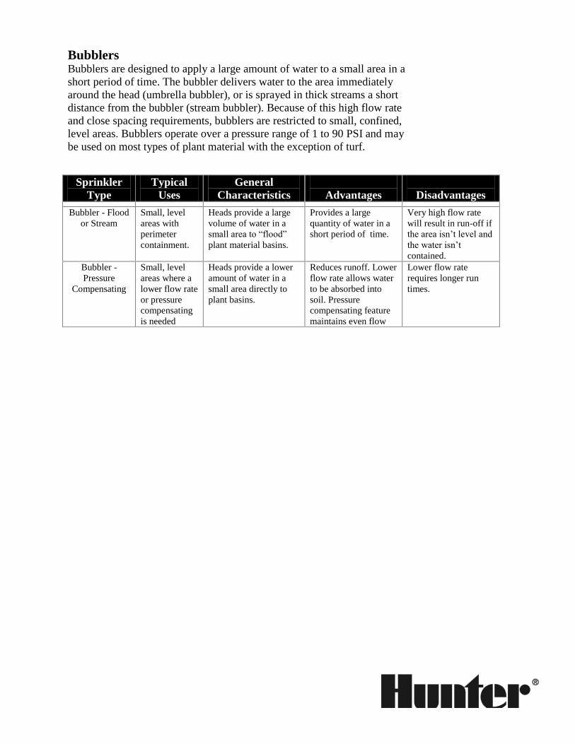
Bubblers Bubblers are designed to apply a large amount of water to a small area in a
short period of time. The bubbler delivers water to the area immediately
around the head (umbrella bubbler), or is sprayed in thick streams a short
distance from the bubbler (stream bubbler). Because of this high flow rate
and close spacing requirements, bubblers are restricted to small, confined,
level areas. Bubblers operate over a pressure range of 1 to 90 PSI and may
be used on most types of plant material with the exception of turf.
Sprinkler
Type
Typical
Uses
General
Characteristics
Advantages
Disadvantages
Bubbler - Flood
or Stream
Small, level
areas with
perimeter
containment.
Heads provide a large
volume of water in a
small area to “flood”
plant material basins.
Provides a large
quantity of water in a
short period of time.
Very high flow rate
will result in run-off if
the area isn’t level and
the water isn’t
contained.
Bubbler -
Pressure
Compensating
Small, level
areas where a
lower flow rate
or pressure
compensating
is needed
Heads provide a lower
amount of water in a
small area directly to
plant basins.
Reduces runoff. Lower
flow rate allows water
to be absorbed into
soil. Pressure
compensating feature
maintains even flow
Lower flow rate
requires longer run
times.
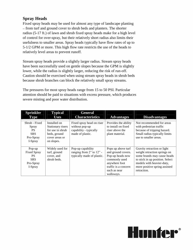
Spray Heads Fixed spray heads may be used for almost any type of landscape planting
– from turf and ground cover to shrub beds and planters. The shorter
radius (5-17 ft.) of lawn and shrub fixed spray heads make for a high level
of control for over-spray, but their relatively short radius also limits their
usefulness to smaller areas. Spray heads typically have flow rates of up to
5-1/2 GPM or more. This high flow rate restricts the use of the heads to
relatively level areas to prevent runoff.
Stream spray heads provide a slightly larger radius. Stream spray heads
have been successfully used on gentle slopes because the GPM is slightly
lower, while the radius is slightly larger, reducing the risk of run-off.
Caution should be exercised when using stream spray heads in shrub beds
because shrub branches can block the relatively small spray streams.
The pressures for most spray heads range from 15 to 50 PSI. Particular
attention should be paid to situations with excess pressure, which produces
severe misting and poor water distribution.
Sprinkler
Type
Typical
Uses
General
Characteristics
Advantages
Disadvantages
Shrub - Fixed
Spray
PS
SRS
Pro-Spray
I-Spray
Installed on
Stationary risers
for use in shrub
beds, ground
cover areas or
on slopes.
Fixed spray head on riser
without pop-up
capability - typically
made of plastic.
Provides the ability
to install on fixed
riser above the
plant material.
Not recommended for areas
with pedestrian traffic
because of tripping hazard.
Small radius typically limits
use to smaller areas.
Pop-up
Fixed Spray
PS
SRS
Pro-Spray
I-Spray
Widely used for
turf, ground
cover, and
shrub beds.
Pop-up capability
ranging from 2” to 12” -
typically made of plastic.
Pops up above turf
and ground covers.
Pop-up heads now
commonly used
anywhere foot
traffic is a concern
such as near
walkways.
Gravity retraction or light
weight retraction springs on
some brands may cause heads
to stick in up position. Select
models with heavier-duty,
more positive spring assisted
retraction.
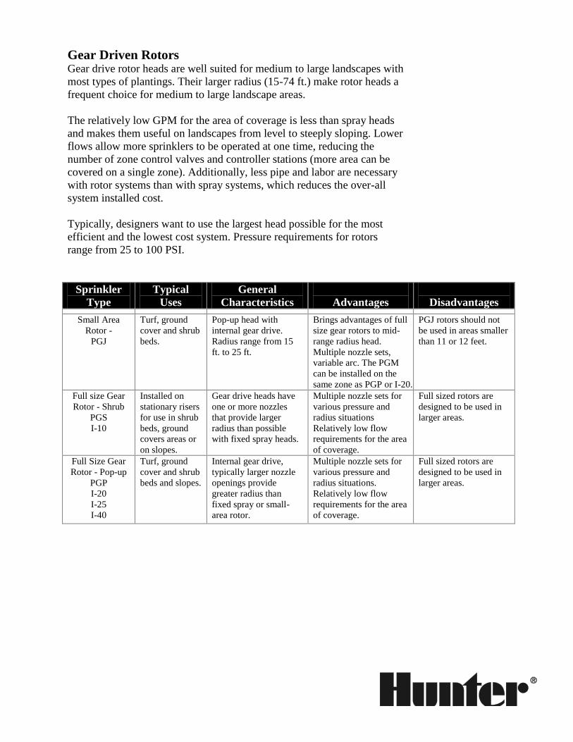
Gear Driven Rotors Gear drive rotor heads are well suited for medium to large landscapes with
most types of plantings. Their larger radius (15-74 ft.) make rotor heads a
frequent choice for medium to large landscape areas.
The relatively low GPM for the area of coverage is less than spray heads
and makes them useful on landscapes from level to steeply sloping. Lower
flows allow more sprinklers to be operated at one time, reducing the
number of zone control valves and controller stations (more area can be
covered on a single zone). Additionally, less pipe and labor are necessary
with rotor systems than with spray systems, which reduces the over-all
system installed cost.
Typically, designers want to use the largest head possible for the most
efficient and the lowest cost system. Pressure requirements for rotors
range from 25 to 100 PSI.
Sprinkler
Type
Typical
Uses
General
Characteristics
Advantages
Disadvantages
Small Area
Rotor -
PGJ
Turf, ground
cover and shrub
beds.
Pop-up head with
internal gear drive.
Radius range from 15
ft. to 25 ft.
Brings advantages of full
size gear rotors to mid-
range radius head.
Multiple nozzle sets,
variable arc. The PGM
can be installed on the
same zone as PGP or I-20.
PGJ rotors should not
be used in areas smaller
than 11 or 12 feet.
Full size Gear
Rotor - Shrub
PGS
I-10
Installed on
stationary risers
for use in shrub
beds, ground
covers areas or
on slopes.
Gear drive heads have
one or more nozzles
that provide larger
radius than possible
with fixed spray heads.
Multiple nozzle sets for
various pressure and
radius situations
Relatively low flow
requirements for the area
of coverage.
Full sized rotors are
designed to be used in
larger areas.
Full Size Gear
Rotor - Pop-up
PGP
I-20
I-25
I-40
Turf, ground
cover and shrub
beds and slopes.
Internal gear drive,
typically larger nozzle
openings provide
greater radius than
fixed spray or small-
area rotor.
Multiple nozzle sets for
various pressure and
radius situations.
Relatively low flow
requirements for the area
of coverage.
Full sized rotors are
designed to be used in
larger areas.
Selecting the Proper Sprinkler Now that you have an understanding of the three categories of sprinklers
available, selecting the proper sprinkler for a project is simply a matter of
analyzing the project and the areas to be watered.
The following are general rules-of-thumb for sprinkler selection.
Remember, there will always be exceptions to these guidelines.
1) Pressure Limitations
2) Flow Limitations
3) Precipitation Rate
4) Large to Small Radius
5) Spray Patterns
6) Angles of Trajectory
7) Special Features
Pressure Limitations The first consideration when choosing the correct sprinkler for an area is
pressure. If the sprinkler’s operating pressure is greater than the estimated
dynamic pressure available (estimated dynamic pressure is discussed in
the Design Capacity section of this manual) the sprinkler must be
eliminated from the list of sprinklers to use. For example, our project has
an estimated dynamic pressure of 50 PSI. For the larger area on this
project, any sprinkler that has an operating pressure over 50 PSI for the 35
ft. radius needed would be scratched from the list of available sprinklers.
Operating Pressure and Head Selection. The operating pressure is the
pressure range that provides optimum sprinkler performance. Hunter
establishes the range of operating pressures for our sprinklers and
publishes those specifications in our catalogs and other product literature.
When selecting a sprinkler the operating pressure must be less than the
estimated dynamic pressure available for the project. Operating pressures
range from as low as 1 to 2 PSI for some bubbler heads to as high as 100
PSI in large turf rotor heads.
Too Little or Too Much Pressure. Attempting to use sprinklers for
which there is insufficient pressure results in distorted spray patterns or
failure of the sprinkler to operate. Applying too much pressure to a head
can cause fogging, misting or structural damage to the sprinkler head. In
general, it is easier to deal with a system that has too much pressure than
one with insufficient pressure. Operating pressures that are too high or too
low will result in uneven water distribution and poor plant growth.
What To Do for Insufficient Pressure. When insufficient pressure is
available for the sprinkler head chosen, there are several alternatives:
check system pressure losses to determine if sufficient pressure can
be conserved elsewhere in the system
select an alternative nozzle for the sprinkler that operates at a lower
pressure (Note: this may affect head spacing and layout)
select an alternative sprinkler model with a lower operating pressure
install a booster pump (Note: this is usually the last choice because
of the high initial cost and continuing operating expenses associated
with booster pumps.)
What To Do With Too Much Pressure. When there is too much
pressure, the pressure may be reduced with a pressure regulator for the
entire system, or with a pressure regulator built into the control valve
(such as Hunter’s ICV). In many cases, minor pressure reductions may be
made using the valve’s flow control.
Flow Limitations The “Design Capacity” that was determined earlier may limit the selection
further. For example: our project has a design capacity of 14 GPM.
Efficient irrigation designs will usually have at least 3 or more heads per
control valve. Using that rule-of-thumb, 14 GPM divided by 3 equals 4.6
GPM as the maximum GPM per sprinkler. Those sprinklers or nozzles
with flow rates in excess of 4.6 GPM should be dropped from
consideration.
Sprinkler Flow Rates and Head Selection. In irrigation system design,
the water available for irrigation on a project is limited to the design
capacity. Once the amount of available water (design capacity) is
established, sprinkler heads that have flow rates of one third the design
capacity or less are selected. The flow rates are published in Hunter’s
catalogs and specification sheets. These flow rates will vary for each type
of sprinkler depending on the operating pressure. It is important to
remember the pressure being used for the design should be no more than
the estimated pressure from the design capacity worksheet.
Selecting sprinklers with flow rates of 1/3 or less of design capacity allows
the use of at least three heads per control valve. This reduces system cost
by keeping the number of control valves to a minimum. For example: if
the design capacity for a project is 18 GPM, sprinklers with a flow rate of
6 GPM or less would be preferred (3 heads x 6 GPM = 18 GPM, which is
within the 1/3 range of the design capacity). There are exceptions to this
general rule, but in most cases, if there are less than three heads per
control valve the system cost will increase substantially.

Precipitation Rate Expressed in inches per hour (in/hr), precipitation rate is the rate at which
water is being applied. Large area rotors and small area sprays may use the
same GPM, but because the size of the areas they cover are not the same,
the inches per hour of water applied is very different. Precipitation rate
affects sprinkler selection and irrigation scheduling. Site conditions,
including slopes or slow soil infiltration rates, may require low
precipitation rate heads or nozzles (less than 0.50 in./hr.). If low
precipitation rates are necessary for the area, eliminate the higher
precipitation rate heads.
Precipitation Rate and Runoff. Caution must be used when selecting
high precipitation rate sprinklers (over 1.0 in./hr.) for use on areas with
slopes. Precipitation rates that exceed soil infiltration rates on sloping soils
can result in runoff. While it is not always possible to select a sprinkler
with a precipitation rate lower than soil infiltration rate, low precipitation
rate sprinklers will reduce the potential for runoff and allow longer run
times per cycle.
Sprinklers are generally described as either :
• Low Precipitation Rate - Less than 0.50 in/hr
• Moderate Precipitation Rate - 0.50 to 1.0 in/hr
• High Precipitation Rate - More than 1.0 in/hr
The chart below shows the range of precipitation rates found in common
sprinkler types. Sprinkler types may fall into more than one category
depending on the nozzle selected.
TYPICAL PRECIPITATION RATE RANGES
LOW MODERATE HIGH
BUBBLERS 1-1/2 to 12 in./hr.
FIXED SPRAYS 1 to 5 in./hr.
GEAR DRIVE ROTORS 0.1 to 1.0 in./hr.
0.1 1.0 2.0
Precipitation Rate versus Sprinkler Run Time. In discussions of
precipitation there is often a misconception about longer run times
associated with low precipitation rate sprinklers. The amount of time
required to irrigate a project is not typically affected by the sprinkler
precipitation rate. While it is true that each low precipitation rate head
must be run for a longer period of time, more heads can be installed on a
zone and, therefore, the total irrigation time for an entire project will be
the same for high precipitation-rate heads with many zones, and low
precipitation-rate heads with few zones.
Rule: Never install sprinklers with different
precipitation rates on the same zone.
Similar run times can be confirmed by checking the design capacity. If
designs with both high and low precipitation-rate heads use the maximum
flow rate available for the project (design capacity) then both projects will
have similar total run times.
Sprinkler Radius Distance of throw is one of the most important criteria in sprinkler
selection. Since the area to be irrigated cannot be changed, the sprinklers
must fit the area. It is usually more cost effective to use fewer sprinklers,
so the sprinklers with the largest radius that can be used is a major
consideration. For example, when the smaller of the two dimensions of an
area to be watered is 35 feet, a sprinkler with a radius that cannot be
adjusted to 35 feet or less would be deleted from the list of possible heads
for the area.
Head Selection Criteria With Regard to Radius. The following
questions should be answered in order to select the best sprinkler for a
project.
What is the largest radius head that can be used in this area?
Is the perimeter straight or curved and irregular?
Is there sufficient pressure to operate large radius sprinkler heads?
Large Radius vs. Small Radius Sprinklers. As a general rule, using
large radius sprinklers on a project will result in less initial system cost.
For example using several valves and numerous 15 ft. radius fixed spray
heads on a football field would be considerably more expensive than using
half-a-dozen valves and a few 60 ft. radius full-size gear drive rotors.
Since using the head with the largest possible radius generally saves
money on system installation, one of the main steps in selecting a
sprinkler is to determine the largest sprinkler radius that can be used on
the area without excessive over-spray; small radius sprinklers tend to
provide coverage with less over-spray in small areas or areas with
irregular perimeters. To determine the largest radius that can be used in an
area, the dimension of the shorter side should be considered.
Generally, for larger areas a larger radius sprinkler is chosen. In some
cases, large areas with irregular perimeters may have large radius
sprinklers in the interior with smaller radius sprinklers along the edges.
If the sprinklers in the smaller areas have a different precipitation rate than
those in the larger area they must be valved separately so sprinkler run
times can be adjusted to provide equal water application.
The range of radius covered is, in part, determined by the type of
sprinkler. Small area spray heads are limited to about 17 feet while full
sized gear rotors have a radius range of up to 100 feet.

Sprinkler Watering Patterns Most sprinklers distribute water in a circular pattern. For these sprinklers
the “pattern” refers to the portion of a circle covered by the sprinkler. The
spray patterns typically available for sprinklers are as follows:
1) Fixed Arc - The fixed arc patterns are set portions of a circle
such as: full is 360°; three-quarter is 270°; two-thirds is 240°; half is 180°;
one-third is 120°; and quarter is 90°. Some manufacturers include other
arcs in addition to these common patterns while other sprinklers may not
be available in as many settings.
2) Adjustable Arc - Adjustable arc sprinklers can be adjusted to
accommodate any landscape including the popular meandering, or curved
lawns and ground covers. Hunter’s adjustable arc patterns are available in
either the smaller area spray sprinklers or the larger area gear drive rotors.
This adjustable arc feature provides additional flexibility in obtaining
coverage in odd shaped landscape areas.
Many contractors now use 100% adjustable arc products on their sites to
assure custom-tailored watering and to reduce the need to stock multiple
parts.
3) Strip Spray Patterns - Fixed pattern spray heads are also
available in rectangular patterns. While a rectangular pattern may seem
ideal for small, narrow landscape areas it is difficult to maintain
satisfactory water distribution when using strip spray heads. These heads
should be used with this potential drawback in mind.
4) Stream Spray Patterns - Stream sprays distribute the water as
small distinct streams as opposed to solid spray patterns. The advantage of
the stream spray is a lower precipitation and flow rate as well as a slightly
larger radius than fixed spray heads. Caution should be used where plant
material might disrupt the small streams.
Angles of Trajectory The trajectory range for most sprinklers is from 0° to 35°. Hunter offers
sprinklers with standard trajectories ranging from 18° to 28° and low angle
trajectories from 13° to 15°, depending on the model sprinkler. Some
considerations for choosing low angle trajectory sprinklers are as follows:
1) Distance of throw - Low angle heads typically have a smaller
radius and higher precipitation rate than standard trajectories for the same
head or nozzle.
2) Wind - The amount of spray pattern distortion caused by wind is
less with a low angle head than one with a standard trajectory.
3) Spraying under barriers - Low angle heads are sometimes used
where the objective is to have the spray pattern below the low hanging
branches and foliage of trees or large shrubs.
Special Sprinkler Features Many times the installation will require a sprinkler with a special feature
such as side inlets, variable arcs, or a built-in check valve to reduce low
head drainage. The following are some of the most popular special
features on many sprinklers and should be reviewed when choosing
sprinklers.
Built-in Check Valves - This feature will prevent water drainage or
puddling at heads located at the lowest elevation on the circuit or zone.
Check valves in these sprinklers typically provide low head drainage
protection for heads from 7 to 15 feet below the highest head.
Reclaimed Water Identifier - Purple identification caps may be
added to identify the sprinkler water source as reclaimed water.
Built-in Filter - Filters built into the body of the sprinkler are common
in sprinklers with small water flows or small orifices.
Multiple Pop-up Heights - The choice of sprinkler pop-up heights
allows selection of a pop-up height from 2 inches to 12 inches. Higher
pop-up heights facilitate irrigating in ground covers or low shrubs.
Side/Bottom Inlets - On higher pop-up models (typically 6 inch or
more) a side inlet may be available. The side inlet allows the taller
pop-up body to be installed with the lateral line buried at a shallower
depth than the overall height of the sprinkler body.
Adjustable Arc - Adjustable arcs have been standard features of gear
drive and impact drive rotors for years. More recently, manufacturers
have developed adjustable arc spray heads. The adjustable arc reduces
the need for numerous sprinklers of various arc patterns, thereby
simplifying inventories, installation and maintenance.
Adjustable Radius - Most sprinklers are designed with radius
adjustment. Sprinkler radius can be adjusted from 75% to 99% of
normal full radius and is useful in reducing over-spray. A note of
caution: reducing the radius may alter the uniformity of water
distribution.
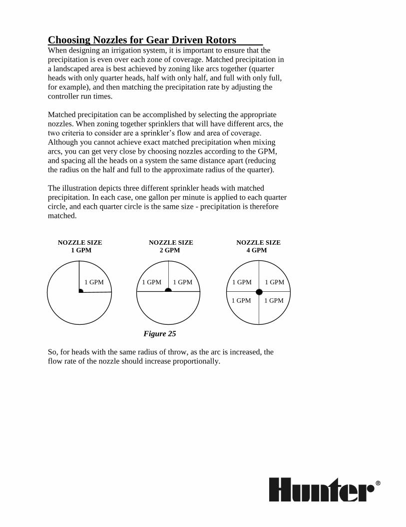
Choosing Nozzles for Gear Driven Rotors When designing an irrigation system, it is important to ensure that the
precipitation is even over each zone of coverage. Matched precipitation in
a landscaped area is best achieved by zoning like arcs together (quarter
heads with only quarter heads, half with only half, and full with only full,
for example), and then matching the precipitation rate by adjusting the
controller run times.
Matched precipitation can be accomplished by selecting the appropriate
nozzles. When zoning together sprinklers that will have different arcs, the
two criteria to consider are a sprinkler’s flow and area of coverage.
Although you cannot achieve exact matched precipitation when mixing
arcs, you can get very close by choosing nozzles according to the GPM,
and spacing all the heads on a system the same distance apart (reducing
the radius on the half and full to the approximate radius of the quarter).
The illustration depicts three different sprinkler heads with matched
precipitation. In each case, one gallon per minute is applied to each quarter
circle, and each quarter circle is the same size - precipitation is therefore
matched.
NOZZLE SIZE NOZZLE SIZE NOZZLE SIZE
1 GPM 2 GPM 4 GPM
1 GPM 1 GPM 1 GPM 1 GPM 1 GPM
1 GPM 1 GPM
Figure 25
So, for heads with the same radius of throw, as the arc is increased, the
flow rate of the nozzle should increase proportionally.
For nozzle selection in areas that will require odd arcs, such as 35º or 270º,
use the following formula.
GPMU = (ARCU/ARCK) x GPMK
Where:
GPMU is the flow rate (in GPM) of the unknown head
ARCU is the arc (in degrees) of the unknown head
ARCK is the arc (in degrees) of the known head
GPMK is the flow rate (in GPM) of the known head
Precipitation rates will be more thoroughly discussed in a later section.
Summary The list of sprinklers available for designing a sprinkler system is huge.
Throughout this section we have discussed various criteria for selecting
the proper sprinkler for a particular use.
Use the product catalog and the following seven points to choose
sprinklers. Remember, these are general rules-of-thumb; there will always
exceptions to these guidelines.
1) Pressure Limitations - If the sprinkler’s operating pressure is greater
than the estimated dynamic pressures available, the sprinkler must be
eliminated from the list of sprinklers to use. On higher pressure
projects, pressure regulation may be necessary.
2) Flow Limitations - The Design Capacity that was determined earlier
may limit the selection further. Efficient irrigation designs will usually
have at least 3 or more heads per control valve. Using that rule-of-
thumb, those sprinklers (or nozzles)with flow rates in excess of 1/3 of
the design capacity should be dropped from consideration.
3) Precipitation Rate - Site conditions including slope and slow soil
infiltration rates may require low precipitation rates (less than 0.50
in./hr.). If low precipitation rates are necessary for the area, eliminate
the high precipitation rate heads such as sprays.
4) Sprinkler Radius - Since it is usually more cost effective to use less
sprinklers, the sprinklers with the largest radius that can be
accommodated in an area are considered first. Sprinklers with a radius
that cannot be adjusted to the shortest distance in an area would not be
placed on the list of possible heads for that area. (Large area rotors are
typically used in areas that are larger than 25 feet, while small area
rotors and sprays are usually placed in areas smaller than 25 feet.)

5) Sprinkler Watering Patterns - Be sure all heads remaining on the list
have the necessary spray patterns for the area being watered.
6) Trajectory - If flat or low angle trajectories are necessary, further
limit the list to those heads with optional low angle trajectories.
7) Special Sprinkler Features - The remaining heads should be
reviewed to check for those needed special features such as side inlets,
variable arcs or built-in check valves.
The list of sprinklers that meet the needed criteria for the area has now
been narrowed to only the appropriate heads. Selection at this point will
depend on your past experience, manufacturer warranty and support, and
project budget.
The seven step checklist approach to head selection will take less time as
you gain experience. With the added experience, you will often know the
sprinkler to choose for a given area from the first glance at a design.
What You Need to Know Do not exceed the systems pressure or flow limitations when choosing
sprinklers.
Never mix sprinklers with different precipitation rates on the same
zone.
Consider the sprinkler’s precipitation rate verses the soil’s infiltration
rate when choosing heads.
Use the largest sprinkler available to cover the area. Using too many
heads unnecessarily increases installation costs, while using too few
heads leads to poor results and inadequate coverage in dry periods.
The adjustable arc reduces the need for numerous sprinklers of various
arc patterns, thereby simplifying inventories, installation and
maintenance.
Use sprinklers with low angle trajectories in areas where wind can be a
problem, or where it is necessary to spray under low growing tree
branches.

Sprinkler Placement Introduction The importance of proper sprinkler placement can not be over-
emphasized. Once installed, if an irrigation system performs inefficiently,
changing the nozzles or even the sprinklers may not be sufficient to
correct the problem. And changing the sprinkler spacing after installation
requires a great deal of additional time and money.
This section is designed to give an overview of head placement. Because
design criteria and preferences vary from one geographical region to the
next, no two designers will arrive at exactly the same placement pattern.
The design criteria on some projects may emphasize sprinkler uniformity
with minimal overspray while other projects may not be as concerned with
uniformity and overspray as with system installation cost. Because of the
varying design criteria and designer preferences, this section will provide
a starting point for learning the art and science of head placement.
Key Factors
While there are different approaches to sprinkler head layout and spacing,
certain factors must be considered for any placement plan. Key among
these is the type and size of the planting areas (also called hydrozones),
the manufacturer’s maximum spacing ratings and the designers choice of
spacing methods, and the effect of wind on those spacing values.
Hydrozones A hydrozone is a portion of the landscape that has similar plants and/or
water requirements. The hydrozone is irrigated by one or more valves
using a common irrigation schedule. Before head placement can begin the
designer must establish hydrozones, or areas with plants that would
logically be watered on a similar irrigation schedule. Examples of
hydrozones include an area of turf grass, a shrub bed, or a slope with
ground cover.
The purpose of establishing hydrozones is to divide the landscape into
areas that would use similar sprinkler equipment and can later be
subdivided into circuits or zones. These circuits or zones are areas with the
identical irrigation requirements. Subdividing the hydrozone into circuits
or zones is presented later in the System Layout section. Once the
hydrozones are established, the process of head spacing and layout begins.
Maximum Spacing Ratings
Traditional head spacing methods try to balance the need for uniform
coverage and sufficient sprinkler overlap with the financial advantage
gained by installing the fewest number of heads possible. This usually
means installing the sprinkler with largest radius possible. (Large area
rotors are typically used in areas that are larger than 15 feet, while small
area sprays are usually placed in areas smaller than 15 feet.) The
recommended sprinkler radius information is found in the Hunter
Irrigation Products Catalog.
The traditional spacing methods are based on either square or triangular
spacing patterns. The distance between sprinklers in a row and the
distance between rows of sprinklers is based on the sprinkler’s radius of
throw. The distance is reduced as the average wind speed increases or as
required by the distribution pattern of the sprinkler.

Square Spacing Patterns In a square spacing pattern the sprinklers in a row are the same distance
apart as the rows of sprinklers. It is sometimes considered that square
spacing provides less uniform coverage than equilateral triangle spacing.
However, in many small landscape areas it provides the best protection
against overspray, and therefore is the preferred spacing pattern.
Figure 26
Triangular Spacing Patterns In a triangular spacing pattern, the heads are placed at the corners of an
equilateral triangle as shown. With triangular head spacing, the uniformity
of coverage will be slightly higher than with square spacing patterns.
Figure 27
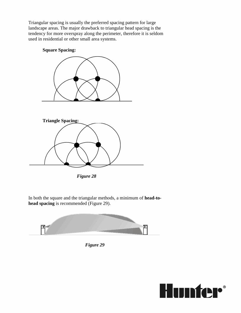
Triangular spacing is usually the preferred spacing pattern for large
landscape areas. The major drawback to triangular head spacing is the
tendency for more overspray along the perimeter, therefore it is seldom
used in residential or other small area systems.
Square Spacing:
Triangle Spacing:
Figure 28
In both the square and the triangular methods, a minimum of head-to-
head spacing is recommended (Figure 29).
Figure 29
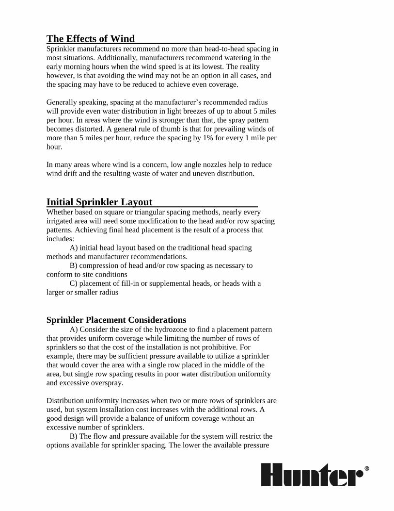
The Effects of Wind
Sprinkler manufacturers recommend no more than head-to-head spacing in
most situations. Additionally, manufacturers recommend watering in the
early morning hours when the wind speed is at its lowest. The reality
however, is that avoiding the wind may not be an option in all cases, and
the spacing may have to be reduced to achieve even coverage.
Generally speaking, spacing at the manufacturer’s recommended radius
will provide even water distribution in light breezes of up to about 5 miles
per hour. In areas where the wind is stronger than that, the spray pattern
becomes distorted. A general rule of thumb is that for prevailing winds of
more than 5 miles per hour, reduce the spacing by 1% for every 1 mile per
hour.
In many areas where wind is a concern, low angle nozzles help to reduce
wind drift and the resulting waste of water and uneven distribution.
Initial Sprinkler Layout Whether based on square or triangular spacing methods, nearly every
irrigated area will need some modification to the head and/or row spacing
patterns. Achieving final head placement is the result of a process that
includes:
A) initial head layout based on the traditional head spacing
methods and manufacturer recommendations.
B) compression of head and/or row spacing as necessary to
conform to site conditions
C) placement of fill-in or supplemental heads, or heads with a
larger or smaller radius
Sprinkler Placement Considerations A) Consider the size of the hydrozone to find a placement pattern
that provides uniform coverage while limiting the number of rows of
sprinklers so that the cost of the installation is not prohibitive. For
example, there may be sufficient pressure available to utilize a sprinkler
that would cover the area with a single row placed in the middle of the
area, but single row spacing results in poor water distribution uniformity
and excessive overspray.
Distribution uniformity increases when two or more rows of sprinklers are
used, but system installation cost increases with the additional rows. A
good design will provide a balance of uniform coverage without an
excessive number of sprinklers.
B) The flow and pressure available for the system will restrict the
options available for sprinkler spacing. The lower the available pressure
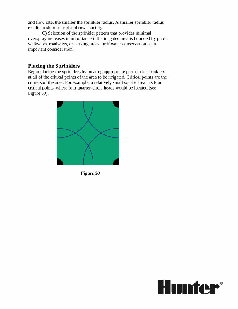
and flow rate, the smaller the sprinkler radius. A smaller sprinkler radius
results in shorter head and row spacing.
C) Selection of the sprinkler pattern that provides minimal
overspray increases in importance if the irrigated area is bounded by public
walkways, roadways, or parking areas, or if water conservation is an
important consideration.
Placing the Sprinklers Begin placing the sprinklers by locating appropriate part-circle sprinklers
at all of the critical points of the area to be irrigated. Critical points are the
corners of the area. For example, a relatively small square area has four
critical points, where four quarter-circle heads would be located (see
Figure 30).
Figure 30
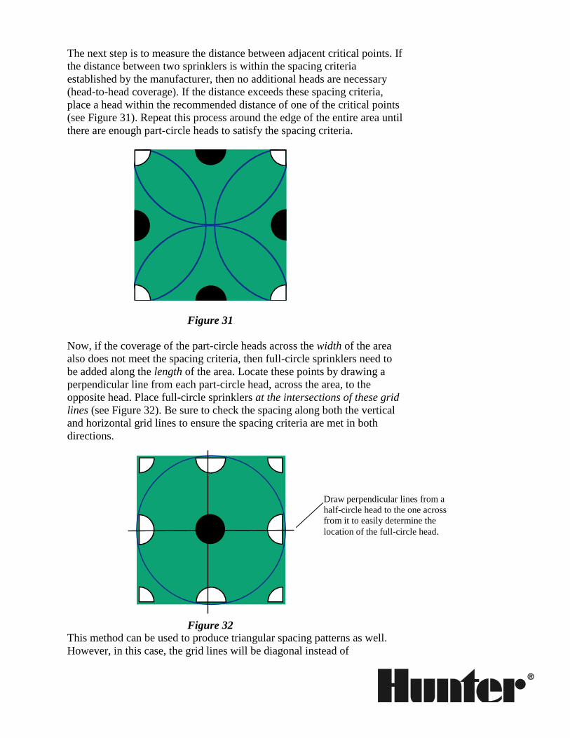
The next step is to measure the distance between adjacent critical points. If
the distance between two sprinklers is within the spacing criteria
established by the manufacturer, then no additional heads are necessary
(head-to-head coverage). If the distance exceeds these spacing criteria,
place a head within the recommended distance of one of the critical points
(see Figure 31). Repeat this process around the edge of the entire area until
there are enough part-circle heads to satisfy the spacing criteria.
Figure 31
Now, if the coverage of the part-circle heads across the width of the area
also does not meet the spacing criteria, then full-circle sprinklers need to
be added along the length of the area. Locate these points by drawing a
perpendicular line from each part-circle head, across the area, to the
opposite head. Place full-circle sprinklers at the intersections of these grid
lines (see Figure 32). Be sure to check the spacing along both the vertical
and horizontal grid lines to ensure the spacing criteria are met in both
directions.
Figure 32
This method can be used to produce triangular spacing patterns as well.
However, in this case, the grid lines will be diagonal instead of
Draw perpendicular lines from a
half-circle head to the one across
from it to easily determine the
location of the full-circle head.
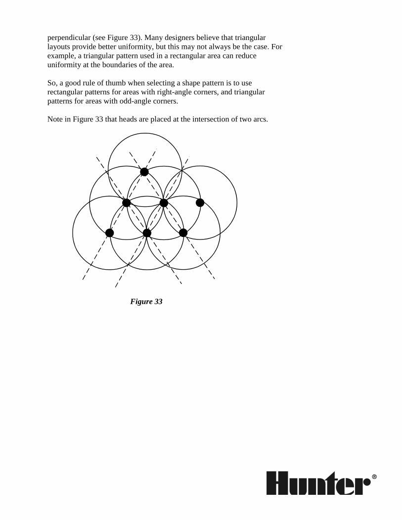
perpendicular (see Figure 33). Many designers believe that triangular
layouts provide better uniformity, but this may not always be the case. For
example, a triangular pattern used in a rectangular area can reduce
uniformity at the boundaries of the area.
So, a good rule of thumb when selecting a shape pattern is to use
rectangular patterns for areas with right-angle corners, and triangular
patterns for areas with odd-angle corners.
Note in Figure 33 that heads are placed at the intersection of two arcs.
Figure 33
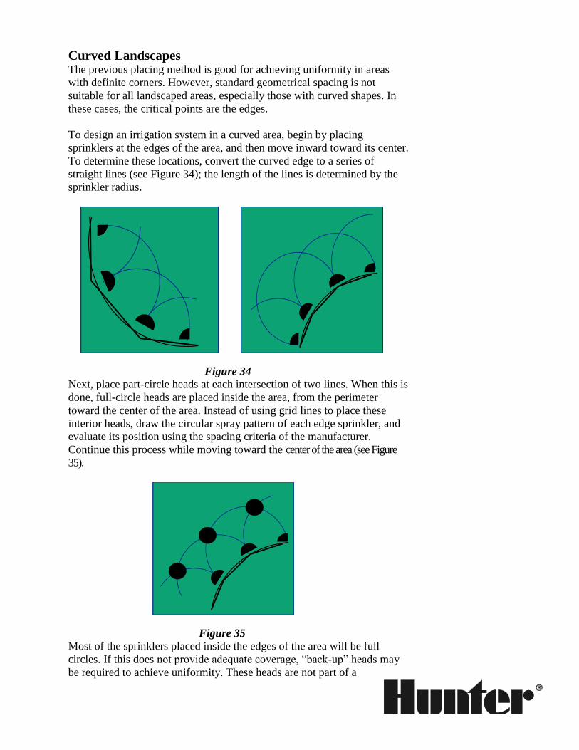
Curved Landscapes The previous placing method is good for achieving uniformity in areas
with definite corners. However, standard geometrical spacing is not
suitable for all landscaped areas, especially those with curved shapes. In
these cases, the critical points are the edges.
To design an irrigation system in a curved area, begin by placing
sprinklers at the edges of the area, and then move inward toward its center.
To determine these locations, convert the curved edge to a series of
straight lines (see Figure 34); the length of the lines is determined by the
sprinkler radius.
Figure 34 Next, place part-circle heads at each intersection of two lines. When this is
done, full-circle heads are placed inside the area, from the perimeter
toward the center of the area. Instead of using grid lines to place these
interior heads, draw the circular spray pattern of each edge sprinkler, and
evaluate its position using the spacing criteria of the manufacturer.
Continue this process while moving toward the center of the area (see Figure
35).
Figure 35
Most of the sprinklers placed inside the edges of the area will be full
circles. If this does not provide adequate coverage, “back-up” heads may
be required to achieve uniformity. These heads are not part of a

“symmetrical” layout, and they are placed to water areas that do not
receive sufficient overlapping coverage from the other sprinklers.
Square, rectangular, and slightly curving landscape areas with no
obstructions are the exception rather than the rule. Most landscape areas
contain curves, obstructions, or size variations that make head placement
more challenging. No two designers approach head placement for an area
in the same way. With that in mind, the following are some typical
problems faced by irrigation designers.
Solutions to the Design Problems There are many solutions to every design problem. All of the solutions,
however, will be undesirable to some degree depending on the design
criteria.
When designing for minimum cost, uniformity is jeopardized.
When trying to reduce head count, overspray becomes a
concern.
Designing for maximum coverage with minimal overspray
results in additional sprinklers and higher installation cost
(lower operating costs may offset higher installation costs
where water rates are high).
Sprinkler head layout is a process of selecting between conflicting design
criteria and reaching a compromise. The following design solutions
emphasize minimal overspray and maximum uniformity at the expense of
additional sprinklers and higher initial expense.
Special Situations Shrub Beds - Shrub beds where plants are spaced close together present
the designer with the problem of dense foliage which blocks spray
patterns.
With dense shrub beds the design options include: 1) shrub heads on tall
risers to spray top of the foliage, 2) low angle trajectory nozzles to spray
under the foliage, 3) bubblers in level areas with contained borders, or 4)
drip irrigation. All of these solutions have their own limitations but
represent possible options.
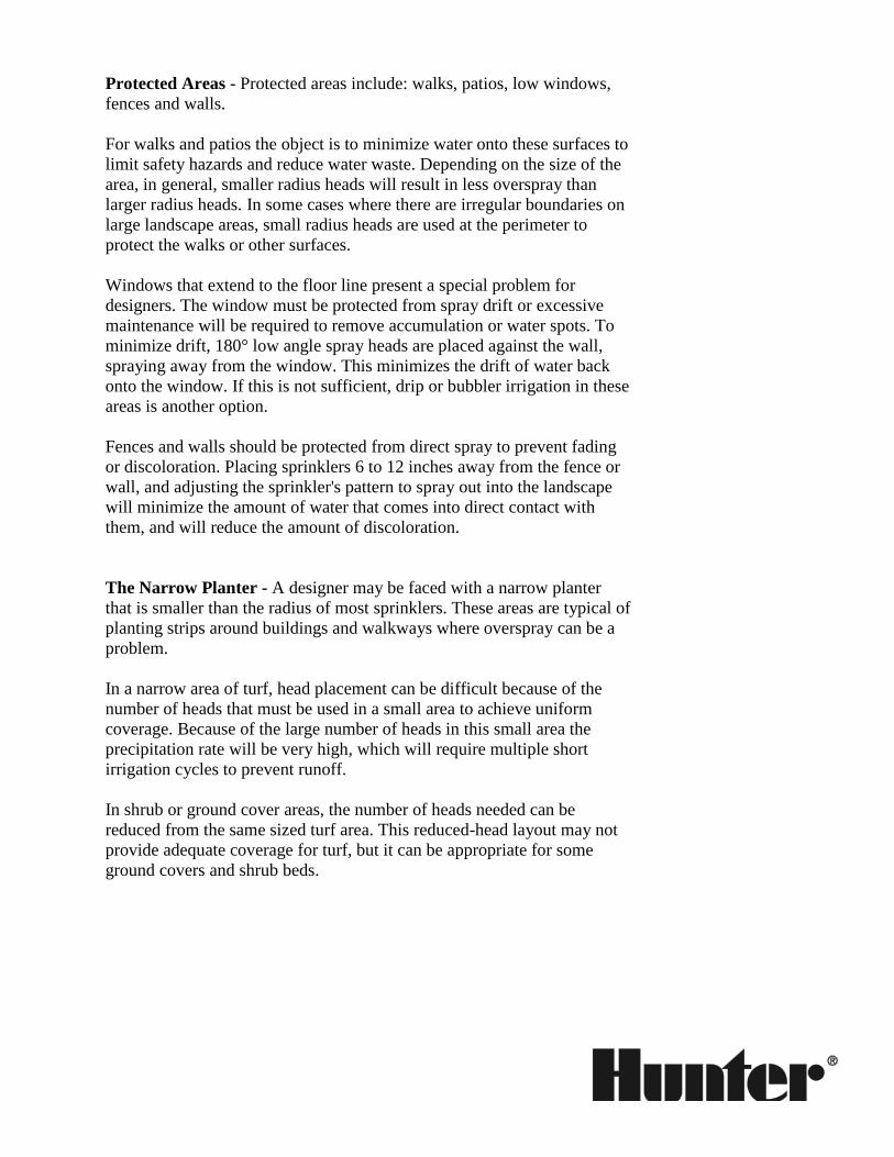
Protected Areas - Protected areas include: walks, patios, low windows,
fences and walls.
For walks and patios the object is to minimize water onto these surfaces to
limit safety hazards and reduce water waste. Depending on the size of the
area, in general, smaller radius heads will result in less overspray than
larger radius heads. In some cases where there are irregular boundaries on
large landscape areas, small radius heads are used at the perimeter to
protect the walks or other surfaces.
Windows that extend to the floor line present a special problem for
designers. The window must be protected from spray drift or excessive
maintenance will be required to remove accumulation or water spots. To
minimize drift, 180° low angle spray heads are placed against the wall,
spraying away from the window. This minimizes the drift of water back
onto the window. If this is not sufficient, drip or bubbler irrigation in these
areas is another option.
Fences and walls should be protected from direct spray to prevent fading
or discoloration. Placing sprinklers 6 to 12 inches away from the fence or
wall, and adjusting the sprinkler's pattern to spray out into the landscape
will minimize the amount of water that comes into direct contact with
them, and will reduce the amount of discoloration.
The Narrow Planter - A designer may be faced with a narrow planter
that is smaller than the radius of most sprinklers. These areas are typical of
planting strips around buildings and walkways where overspray can be a
problem.
In a narrow area of turf, head placement can be difficult because of the
number of heads that must be used in a small area to achieve uniform
coverage. Because of the large number of heads in this small area the
precipitation rate will be very high, which will require multiple short
irrigation cycles to prevent runoff.
In shrub or ground cover areas, the number of heads needed can be
reduced from the same sized turf area. This reduced-head layout may not
provide adequate coverage for turf, but it can be appropriate for some
ground covers and shrub beds.
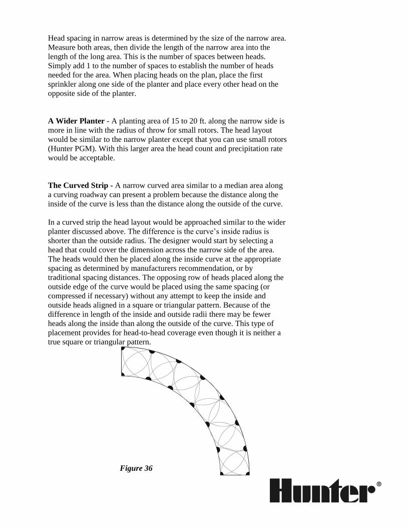
Head spacing in narrow areas is determined by the size of the narrow area.
Measure both areas, then divide the length of the narrow area into the
length of the long area. This is the number of spaces between heads.
Simply add 1 to the number of spaces to establish the number of heads
needed for the area. When placing heads on the plan, place the first
sprinkler along one side of the planter and place every other head on the
opposite side of the planter.
A Wider Planter - A planting area of 15 to 20 ft. along the narrow side is
more in line with the radius of throw for small rotors. The head layout
would be similar to the narrow planter except that you can use small rotors
(Hunter PGM). With this larger area the head count and precipitation rate
would be acceptable.
The Curved Strip - A narrow curved area similar to a median area along
a curving roadway can present a problem because the distance along the
inside of the curve is less than the distance along the outside of the curve.
In a curved strip the head layout would be approached similar to the wider
planter discussed above. The difference is the curve’s inside radius is
shorter than the outside radius. The designer would start by selecting a
head that could cover the dimension across the narrow side of the area.
The heads would then be placed along the inside curve at the appropriate
spacing as determined by manufacturers recommendation, or by
traditional spacing distances. The opposing row of heads placed along the
outside edge of the curve would be placed using the same spacing (or
compressed if necessary) without any attempt to keep the inside and
outside heads aligned in a square or triangular pattern. Because of the
difference in length of the inside and outside radii there may be fewer
heads along the inside than along the outside of the curve. This type of
placement provides for head-to-head coverage even though it is neither a
true square or triangular pattern.
Figure 36
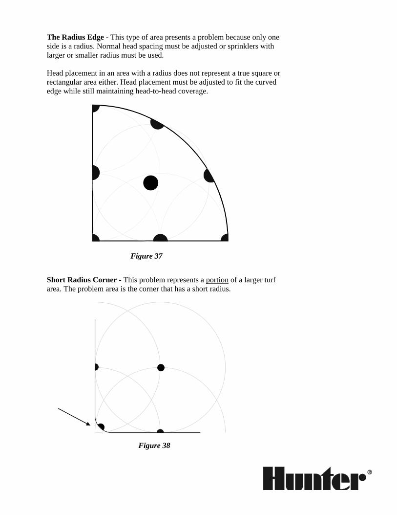
The Radius Edge - This type of area presents a problem because only one
side is a radius. Normal head spacing must be adjusted or sprinklers with
larger or smaller radius must be used.
Head placement in an area with a radius does not represent a true square or
rectangular area either. Head placement must be adjusted to fit the curved
edge while still maintaining head-to-head coverage.
Figure 37
Short Radius Corner - This problem represents a portion of a larger turf
area. The problem area is the corner that has a short radius.
Figure 38
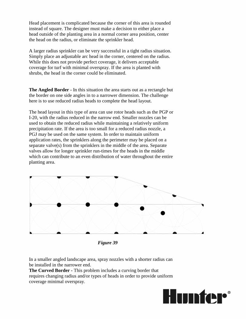
Head placement is complicated because the corner of this area is rounded
instead of square. The designer must make a decision to either place a
head outside of the planting area in a normal corner area position, center
the head on the radius, or eliminate the sprinkler head.
A larger radius sprinkler can be very successful in a tight radius situation.
Simply place an adjustable arc head in the corner, centered on the radius.
While this does not provide perfect coverage, it delivers acceptable
coverage for turf with minimal overspray. If the area is planted with
shrubs, the head in the corner could be eliminated.
The Angled Border - In this situation the area starts out as a rectangle but
the border on one side angles in to a narrower dimension. The challenge
here is to use reduced radius heads to complete the head layout.
The head layout in this type of area can use rotor heads such as the PGP or
I-20, with the radius reduced in the narrow end. Smaller nozzles can be
used to obtain the reduced radius while maintaining a relatively uniform
precipitation rate. If the area is too small for a reduced radius nozzle, a
PGJ may be used on the same system. In order to maintain uniform
application rates, the sprinklers along the perimeter may be placed on a
separate valve(s) from the sprinklers in the middle of the area. Separate
valves allow for longer sprinkler run-times for the heads in the middle
which can contribute to an even distribution of water throughout the entire
planting area.
Figure 39
In a smaller angled landscape area, spray nozzles with a shorter radius can
be installed in the narrower end.
The Curved Border - This problem includes a curving border that
requires changing radius and/or types of heads in order to provide uniform
coverage minimal overspray.

A possible solution for this problem would be to use fixed spray heads
(Hunter PS or SRS) to provide uniform coverage with minimal overspray.
Another solution if the area is large with a tight curved border would be to
use a combination of Hunter PGP or I-20 rotors and PGJ rotors on the
same zone, or even Pro-Spray or I-Spray spray heads on a separate zone
from the rotors. If you would need to use the spray heads, the use of the
rotor heads in the same area substantially reduced the overall cost for the
larger area even though the spray and rotor heads would have to be on
separate valves. The difficult portion of this solution is to decide where to
stop the spray heads and start the rotors.
PGP

Figure 40
PGJ
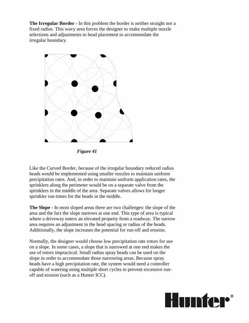
The Irregular Border - In this problem the border is neither straight nor a
fixed radius. This wavy area forces the designer to make multiple nozzle
selections and adjustments to head placement to accommodate the
irregular boundary.
Figure 41
Like the Curved Border, because of the irregular boundary reduced radius
heads would be implemented using smaller nozzles to maintain uniform
precipitation rates. And, in order to maintain uniform application rates, the
sprinklers along the perimeter would be on a separate valve from the
sprinklers in the middle of the area. Separate valves allows for longer
sprinkler run-times for the heads in the middle.
The Slope - In most sloped areas there are two challenges: the slope of the
area and the fact the slope narrows at one end. This type of area is typical
where a driveway enters an elevated property from a roadway. The narrow
area requires an adjustment in the head spacing or radius of the heads.
Additionally, the slope increases the potential for run-off and erosion.
Normally, the designer would choose low precipitation rate rotors for use
on a slope. In some cases, a slope that is narrowed at one end makes the
use of rotors impractical. Small radius spray heads can be used on the
slope in order to accommodate those narrowing areas. Because spray
heads have a high precipitation rate, the system would need a controller
capable of watering using multiple short cycles to prevent excessive run-
off and erosion (such as a Hunter ICC).
On larger slopes, a combination of rotors in the larger areas and sprays in
the smaller areas with separate valves controlling the application of water
can be a possible solution.
In order to provide greater control, three separate valves would be
installed on the slope; one controlling the heads at the top of the slope, one
for the middle heads, and one for the heads at the bottom of the slope.
Obstructions in the Landscape - With obstructions in the landscape,
such as tree trunks, light poles or signs, care must be taken to prevent dry
spots behind the obstruction caused by a blocked spray pattern. When
obstructions are present, design options include: 1) adjusting head
placement so the obstruction is at equal distance between adjoining heads
or, 2) placing an additional fill-in head next to the obstruction spraying
into the area where the spray pattern is blocked or 3) selecting larger
radius heads where pattern is blocked in order to reach the dry spot.
Solutions to the problem of obstructions in the landscape require: 1)
adjusting head placement so the obstruction is at equal distance between
adjoining heads or, 2) placing additional fill-in heads near the obstruction
spraying into the area where the spray pattern is blocked or, 3) selecting
larger radius heads where pattern is blocked to reach the dry spot.
Residential Landscape: Adjoining Large and Small Areas - With this
residential yard the designer is presented with the typical problem of a
lawn area that has a small narrow area attached to a larger lawn area. In
these situations, the designer must either maintain uniform precipitation
rates in the large and small areas or separate valves must be used to
accommodate the different precipitation rates when using different types
of heads.
The small and large adjoining areas problem presents a difficult design
situation which is common on small residential areas. The designer is
faced with: 1) turf areas with east and west exposure which will require
different irrigation schedules, 2) large and small turf areas that require
different sprinkler types, 3) challenges to maintain uniform coverage with
minimal overspray.
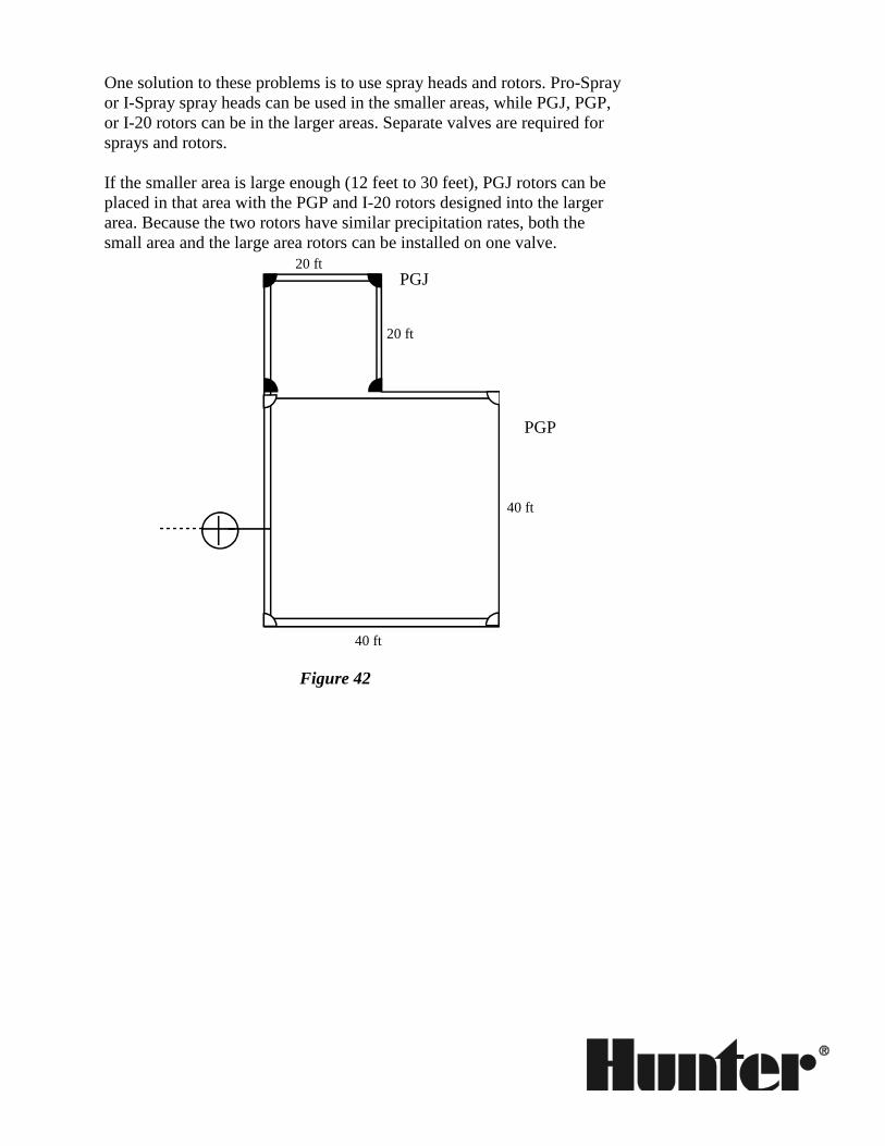
One solution to these problems is to use spray heads and rotors. Pro-Spray
or I-Spray spray heads can be used in the smaller areas, while PGJ, PGP,
or I-20 rotors can be in the larger areas. Separate valves are required for
sprays and rotors.
If the smaller area is large enough (12 feet to 30 feet), PGJ rotors can be
placed in that area with the PGP and I-20 rotors designed into the larger
area. Because the two rotors have similar precipitation rates, both the
small area and the large area rotors can be installed on one valve.
Figure 42
20 ft
20 ft
40 ft
40 ft
PGJ
PGP

Summary Sprinkler head placement is the most difficult and one of the most
important steps in sprinkler system design. System uniformity, and
installation and operating costs are determined by head placement plans.
Improved head placement will occur when:
1. manufacturer’s recommendations are followed
2. careful analysis of head layout is included in the design process
3. head placement plans are compared with field installations
While no head placement plan will result in perfect water distribution
uniformity, well thought out placement patterns will result in improved
system performance and plant health over the lifetime of the irrigation
system.
What You Need to Know
Decide where you will be installing large area sprinklers and where you
will be installing small area sprinklers.
Always design your sprinkler systems with head-to-head coverage.
Design the system by placing sprinklers in one area at a time.
The critical points are the corners. Mark the corners to receive
heads, then using a compass, draw an arc showing the
sprinkler’s pattern.
If the quarter circle heads will not spray each other, place
sprinklers along the perimeters. Draw these sprinkler’s watering
patterns.
If the perimeter heads will not spray across the area to the heads
on the other side, add full circle heads in the middle. Draw these
sprinkler’s watering patterns.
Minimal overspray and maximum uniformity is achieved at the expense
of additional sprinklers and higher initial expense.
Sprinkler head layout is a process of selecting between conflicting design
criteria and reaching a compromise. Your design solutions will be driven
by the budget – with a higher the budget, your design can be more
efficient.
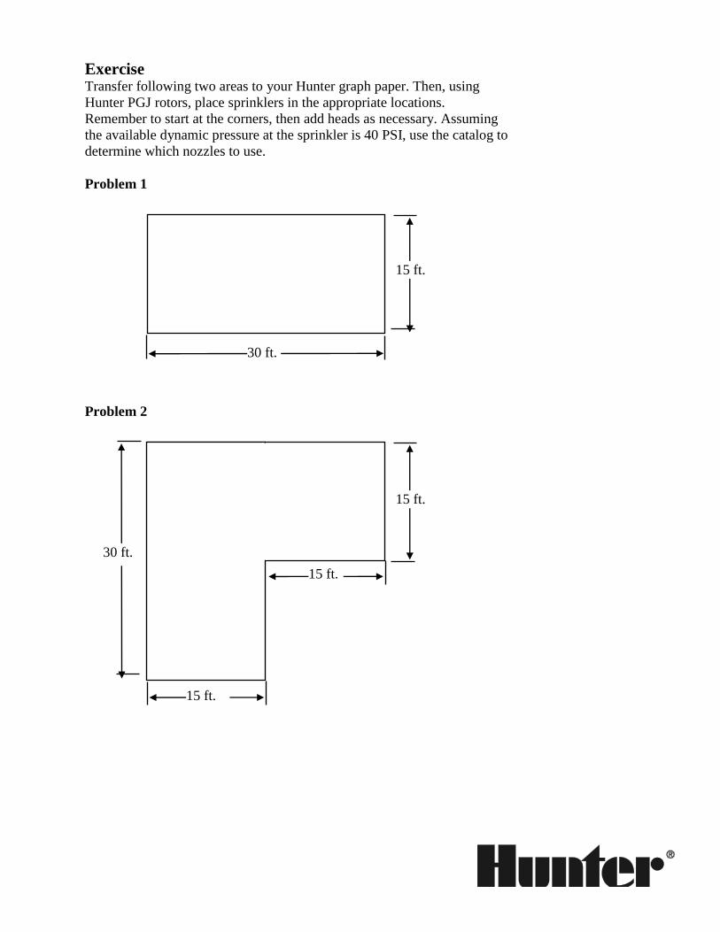
Exercise Transfer following two areas to your Hunter graph paper. Then, using
Hunter PGJ rotors, place sprinklers in the appropriate locations.
Remember to start at the corners, then add heads as necessary. Assuming
the available dynamic pressure at the sprinkler is 40 PSI, use the catalog to
determine which nozzles to use.
Problem 1
Problem 2
30 ft.
15 ft.
15 ft.
15 ft.
15 ft.
30 ft.
Backflow Prevention Introduction Backflow in sprinkler systems is the reversal of the flow of water from the
sprinkler system back into the potable water system. This undesirable
reversal of flow can draw contaminated water back into the drinking water
system. There are many case studies where the backflow of contaminated
water has caused severe and widespread illnesses, and in some cases
deaths.
The intent of this section is to make you aware of the need for backflow
prevention on all projects. Additionally, because you will understand the
need of reducing this risk, you will have a better understanding of proper
installation practices.
The following booklet on backflow preventers is very well written and
includes a thorough discussion of what backflow is, and case studies to
support the use of backflow prevention devices.
Various types of backflow prevention devices are discussed in the booklet.
The Device Selection portion will help you decide which backflow
preventer to use, and the Installation section provides you with details for
the proper installation of each device.
As the various municipalities will require different types of devices, we
recommend that in each separate area where you plan on installing a
sprinkler system, you check the requirements for that area.
System Layout
and Pipe Sizing Introduction Many hydrozone areas on a property will require more water than the
property has available (system design capacity). The design pressure and
flow must not exceed the calculated system design capacity and the
pressure available for sprinkler selection and operation.
When backflow preventers, valves, or main line or lateral line pipe is sized
too small, the system may experience water hammer. Severe water
hammer will cause the pipes to vibrate or create a pounding noise. In
extreme conditions, damage to the system may occur.
When the components are sized too large, the initial cost of the system is
higher than necessary. Automatic control valves which are sized too large
may not close due to the slow moving water.
This section discusses the procedures for correctly laying out and sizing
the pipe and other components that go into a sprinkler system.
System Layout
Laying out a system begins with the information learned in the Sprinkler
Selection and the Sprinkler Placement sections. Once the sprinkler
locations for each hydrozone have been established, circuit the sprinklers
into zones based on the design capacity as determined in the Design
Capacity section. After the individual sprinkler zones have been
established, connect the sprinklers together with pipe, size the pipe, and
layout and size the valves and backflow preventer.
Circuiting Sprinklers Into Zones Dividing the area into zones so that the design capacity is not exceeded is
an easy process.
Working in one area at a time, write individual sprinkler GPM
requirement next to each sprinkler in the area. Add up the GPM
requirements for all sprinklers in one hydrozone, and divide by the total
GPM (Design Capacity) available.
: =
total GPM of all heads in one area design capacity in GPM number of zones in this area
If the “number of zones in this area” is not a whole number, round the
number up to establish how many zones there will be. (1.2 zones becomes
2 zones.) This is the total number of valves needed for the sprinklers in
that area.
If more than one zone will be needed for the area, divide up the sprinklers
so that all zones in the area will have approximately the same GPM flow
requirement. Don’t place too many heads on the same zone; stay within
the system’s design capacity.
Repeat this process for each area on the property.
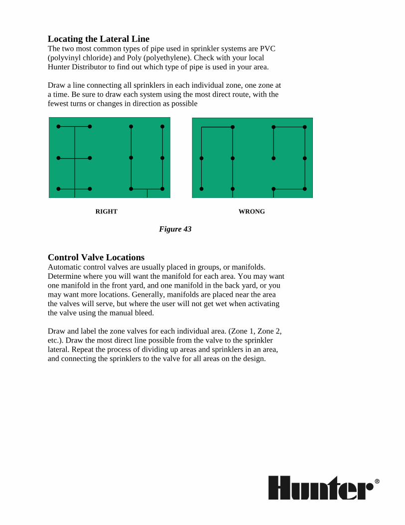
Locating the Lateral Line
The two most common types of pipe used in sprinkler systems are PVC
(polyvinyl chloride) and Poly (polyethylene). Check with your local
Hunter Distributor to find out which type of pipe is used in your area.
Draw a line connecting all sprinklers in each individual zone, one zone at
a time. Be sure to draw each system using the most direct route, with the
fewest turns or changes in direction as possible
RIGHT WRONG
Figure 43
Control Valve Locations Automatic control valves are usually placed in groups, or manifolds.
Determine where you will want the manifold for each area. You may want
one manifold in the front yard, and one manifold in the back yard, or you
may want more locations. Generally, manifolds are placed near the area
the valves will serve, but where the user will not get wet when activating
the valve using the manual bleed.
Draw and label the zone valves for each individual area. (Zone 1, Zone 2,
etc.). Draw the most direct line possible from the valve to the sprinkler
lateral. Repeat the process of dividing up areas and sprinklers in an area,
and connecting the sprinklers to the valve for all areas on the design.

Backflow Preventer Location
Local plumbing codes govern the installation of backflow preventers.
Usually, you will be required to place them in a position on the property
where they are a minimum of 12” above the highest head. Check your
local codes. Draw the location for the backflow preventer on the plan.
Main Line Location
In most systems, the main line will be under continuous pressure. Class
315 or Sch 40 PVC is the most common choice for main line pipe in these
situations.
Determine the location for the point of connection (POC). Draw a line
connecting all of the zone valve manifolds together, and then draw a line
connecting this line to the backflow preventer, and then to the POC.
If the installation is in a freezing climate and the POC is in a basement,
install a gate valve and a boiler drain immediately after the POC to drain
the system in the winter. Install a slip x slip x 1 inch threaded tee with a
riser and a threaded cap after the backflow preventer to be used for
blowing out the system before the first deep freeze.
Copper pipe may be required between the POC and the backflow
preventer. Always check the local plumbing codes for the requirements in
your area. In general, above ground connections to backflow preventers
should use metal pipe and fittings for durability and sunlight resistance.
Isolation Valve Locations
Isolation valves are great to use when performing maintenance on the zone
control valves. On large commercial properties, it is not uncommon to
place an isolation valve at each control valve manifold. On smaller
properties, it is usually sufficient to place one main shutoff valve at the
POC only. Many times, residential designers place isolation valves at the
POC, and at both sides of a tee in a main line system for ease of
maintenance.
Today’s low cost PVC ball valves make isolation valves for residential
installations economically feasible easy to install. Note all isolation valve
locations on the design.
Controller Placement and Wire Routing Controllers (sometimes called clocks) are available in indoor mount and
outdoor mount. Indoor mount controllers such as a Hunter SRC should be
in a weatherproof enclosure or in an indoor location, such as a garage,
shed, or covered porch, which is protected from moisture and direct
sunlight. Outdoor-approved controllers can be mounted outside without an
additional enclosure. An example of an outdoor-approved controller is a
Hunter ICC-PL or a Hunter ICC-M
Indoor controllers should be mounted near a 120 volt AC outlet where the
24 volt plug-in transformer is connected. Outdoor controllers are
frequently “hard wired” from the 120 volt source to the controller location.
Hard wiring often requires the use of conduit – check local electrical codes
for the type of wire and wire conduit to use.
For new construction, the controller location can be pre-planned and the
120 volt wiring can be installed in the wall before the wall is finished. The
wire can then be installed through the back of the controller, in most cases
eliminating the need for a conduit. Note the controller location and the 120
volt source on the plan.
The low voltage wire which runs from the controller to the valves is
usually installed in the main line trench. You may want to indicate wire
runs on your plan.
Wire connectors which are not exposed to moisture can be electrical “wire
nuts” or insulated electrical connectors. Connections that will be located at
the valves or in other areas subject to moisture should always be
waterproof direct burial type. The low voltage control wire running from
the controller to the valves should be rated for direct burial. This type of
wire is available as an insulated single strand or as a jacketed multi-
conductor. Either is acceptable for small irrigation systems, but the
jacketed multi-conductor is generally less expensive.
Remote Control/Remote Programmer
A remote control can save time during installation and routine system
maintenance. A receiver is installed at the controller, and a transmitter
activates the sprinklers from a location on the property some distance from
the controller. This allows the contractor or property owner to remotely
activate a manual watering or system blow-out without the need to visit
the controller.
There are a few different models of remotes available at various price
points. The Hunter ICR receiver is plugged into an easy to hook-up wiring
harness and can be used at up to 450 feet away from the receiver.
Watering can be remotely controlled for all stations, or for one station at a

time. Station run time can be temporarily changed to permit custom
operation. The ICR is very affordable and is available for use on Hunter
SRC and ICC controllers.
Rain Sensor
Rain sensors are small sensing units which collect rainfall. They are used
to stop the controller from sending the low voltage signal to the control
valves during periods of rain.
Rain sensors are usually mounted near the controller on the eaves of a
roof, or on a fence, away from possible irrigation interruption due to
sprinkler water. Be sure to install the sensor away from obstructions so
that rain can freely fall onto the sensor.
If a Hunter controller is not being installed, it is helpful to wire-in a bypass
switch to turn off a sensor when its operation is undesirable (e.g. testing a
system after rainfall). Hunter controllers have a built-in feature to
accommodate this.

Pipe Sizing You are now ready to begin sizing the pipe throughout the system. As
previously mentioned, sizing pipes is a matter of friction loss
management.
In many areas of the country, when installing a sprinkler system on a small
residence, it is a standard practice to use just one size of polyethylene
(poly) or PVC pipe for all lateral lines. This practice saves installation
time, reduces fitting inventory costs, and in most cases will not present
any problems as long as the installer does not exceed the maximum flow
rate for the size of the pipe used.
The larger the project however, the more important it becomes to manage
the system’s friction losses. When installing larger systems, sizing all
lateral lines the same can be quite wasteful. The material costs are higher,
and the amount of water required to fill an over-sized pipe, which is then
lost to low head drainage, can be significant.
Here, we are going to discuss pipe sizing so that you are familiar with the
procedure. Many times when a sprinkler is not performing according to
manufacturer’s specifications, it is because of improper pressure or flow.
Correct pipe sizing will uncover potential pressure or flow problems in
sprinkler systems.
When sizing pipes, you can use the friction loss tables developed from the
Hazen-Williams formula, or you can use the Friction Factor formula.
Pipe Sizing Using the Friction Loss Tables
Lateral Lines. Refer to the Hunter Friction Loss Tables in the back of
this Design Manual and begin sizing the pipe:
1. Start at the head furthest from the zone valve. The pipe
connecting the last head to the second to the last head should be
3/4”. (It is acceptable to use 1/2” PVC pipe, but do so with
caution; watch the sprinkler’s flow requirements.)
2. Add the GPM requirements of the last head and the second to
the last head together to size the next pipe.
3. On the Friction Loss Table for the type of pipe you have
designed, find the GPM total from step 2 in the far left column.
4. On that row, go across to the first column that is not shaded*.
At the top of this column is the pipe size necessary to carry the
flow for these two heads.
5. Add the GPM requirements of the next head to the last GPM
total.
6. Find this total in the Friction Loss Tables.
7. Continue to do this until you get to the zone valve. Do not try to
size a pipe smaller than the chart indicates.
8. Repeat steps 1 through 7 for each zone.
Main Lines. Refer to the Hunter Friction Loss Tables for sizing the main
line. The main line should be sized large enough to handle the
requirements of the zone valves it is serving; use the zone with the largest
flow requirements. (Note: This assumes only one valve will be operating
at one time on an automatic system.)
*Note: The shaded area on the chart designates those flow rates that exceed 5 fps.
It is recommended that caution be used with flow rates exceeding 5 fps in pipes.

Pipe Sizing Using the Friction Factor Formula
The Friction Factor formula is used to determine the maximum flow in
gallons per minute through any section of lateral line pipe while not
exceeding a predetermined pressure loss variation. In order to minimize
uneven distribution, sprinklers on a zone should operate with pressure
variation between sprinklers of not more than
10% to 20 % of the desired sprinkler operating pressure.
Friction Factor = sprinkler operating pressure x allowable % of PSI variation
critical length of pipe from the valve to the furthest head
(in hundreds of feet)
Once the acceptable PSI loss has been calculated, refer to the Hunter
Friction Loss Tables to size the pipe.
1. Beginning with the smallest sized pipe on the friction loss chart
for the pipe you are using, locate the calculated Friction Factor
under the column labeled “P.S.I. LOSS”
2. Now go across the row at this point to the left hand column to
find how much water should be allowed to flow through this
size pipe.
3. Repeat step one and step two for all sizes of pipe until you have
reached your design capacity.
4. Starting at the head furthest from the zone valve, begin sizing
the pipe based on the numbers obtained in steps 1 through 3.
The pipe connecting the last head to the second to the last head
should be 3/4”. (It is acceptable to use 1/2” PVC pipe, but do so
with caution; watch the sprinkler’s flow requirements.)
5. Add the GPM requirements of those two heads together, and
note how it compares to the allowable GPM in steps 1 through
3.
6. Add the GPM requirements of the next head to the last GPM
total. Again note how the total GPM requirement compares to
the allowable GPM in steps 1 through 3.
7. Continue to do this until you get to the zone valve. Do not try to
size a pipe smaller than the Friction Formula indicates.
8. Repeat steps 4 through 7 for each zone.
The Friction Factor formula is the most accurate method of pipe sizing,
and will provide the most uniform application of water. Hunter’s
Handbook of Technical Irrigation Information (LIT-194) has a section
titled Friction Factor Short Cuts. In this section, pipe sizing charts are
provided for various types of pipe and Friction Factors.
Backflow Preventer and Valve Sizing Backflow preventers and automatic control valves can be large pressure
consumers. Sizing these valves is easy – simply use the manufacturer’s
pressure loss charts. Isolation valves can be great tools if valve
maintenance is necessary, and are mandatory for winterization if the
system is installed in freezing climates.
Backflow Preventers
Backflow preventers are generally sized the same size as, or one size
smaller than the mainline. Check the pressure loss chart in the
manufacturer’s product catalog to be sure it is not sized too small. Use
caution when sizing backflow preventers. If they are sized too small, high
friction losses may occur.
Isolation Valve Sizing Isolation valves (gate valves or ball valves) should be line size. In other
words, if the main line is 1”, the isolation valve should be 1”; if the main
line is 1-1/4”, the isolation valve should be 1-1/4”.
Automatic Zone Control Valve Sizing
Size automatic control valves according to the zone flow rate
requirements. Generally speaking, automatic control valves can be sized
as small as one size smaller than the lateral line it is serving. Check the
pressure loss chart in the product catalog to be sure it is not sized too
small. Use caution when sizing control valves. If the valves are sized too
small, high friction losses are inevitable, and water hammer is likely.
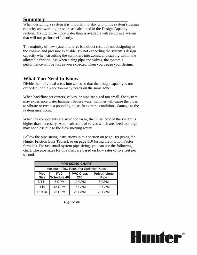
Summary
When designing a system it is important to stay within the system’s design
capacity and working pressure as calculated in the Design Capacity
section. Trying to use more water than is available will result in a system
that will not perform efficiently.
The majority of new system failures is a direct result of not designing to
the volume and pressure available. By not exceeding the system’s design
capacity when circuiting the sprinklers into zones, and staying within the
allowable friction loss when sizing pipe and valves, the system’s
performance will be just as you expected when you began your design.
What You Need to Know
Divide the individual areas into zones so that the design capacity is not
exceeded; don’t place too many heads on the same zone.
When backflow preventers, valves, or pipe are sized too small, the system
may experience water hammer. Severe water hammer will cause the pipes
to vibrate or create a pounding noise. In extreme conditions, damage to the
system may occur.
When the components are sized too large, the initial cost of the system is
higher than necessary. Automatic control valves which are sized too large
may not close due to the slow moving water.
Follow the pipe sizing instructions in this section on page 109 (using the
Hunter Friction Loss Tables), or on page 110 (using the Friction Factor
formula). For fast small-system pipe sizing, you can use the following
chart. The pipe sizes for this chart are based on flow rates of five feet per
second.
PIPE SIZING CHART
Maximum Flow Rates For Sprinkler Pipes
Pipe Size
PVC Schedule 40
PVC Class 200
Polyethylene Pipe
3/4 in. 8 GPM 10 GPM 8 GPM
1 in 13 GPM 16 GPM 13 GPM
1 1/4 in. 23 GPM 26 GPM 23 GPM
Figure 44
Friction Losses Introduction Calculating the friction losses on your design is a critical step in providing
an accurately completed plan. In the Design Capacity section, we
estimated how much pressure would be available at a particular flow. In
the System Layout section, those estimates were used to design the
system. This system design establishes the actual flow that will be used to
water the landscaped area. But remember, the system was designed using
estimates; the plan must be checked to verify that the sprinkler system will
operate as designed.
Excessive friction losses results in a system that may not work efficiently,
or a system that may fail in the future due to pressure changes occurring in
the neighborhood. This section will lead you through the process of
checking the design to make sure that the friction losses will not be
excessive.

Most Critical Zone While checking the friction losses for each zone on the plan is a good
idea, it is not always a requirement. For example, if one zone on the
property has a 15 GPM flow rate, it may not be necessary to check the
zone with a flow rate of 10 GPM.
If, however, the 10 GPM zone is several feet higher than the 15 GPM
zone, then it would be wise to check the friction losses on that zone as
well. Additionally, the zone with the highest flow rate may not be the
furthest away from the POC, and as previously discussed, distance is a
factor in friction losses.
So, when deciding which zone is the most critical zone for calculating
friction losses, consider the following factors:
the most GPM, or highest flow rate
highest head(s)
furthest distance from the POC
This may mean that the friction losses must be calculated on several, or all
of the zones.
Calculating Friction Losses Using the completed plan with the sprinkler’s GPM requirements marked
at each head location, and the Friction Loss Tables located in the back of
this design manual, begin calculating the PSI losses on the critical zones.
Calculate one zone at a time.
PSI Losses in Lateral Line Pipe
Turn to the Hunter Friction Loss Tables in the back of this design
workbook for the type of lateral line pipe used in the design. On the plan,
note the GPM requirement for the last head on the zone that you have
chosen to calculate.
1. Look in the “FLOW G.P.M.” column on the friction loss
chart and read down to the GPM for the last head.
2. Now, read across the top of the chart looking for the size of
the pipe that supplies water to this head.
3. Read down this column, under the “P.S.I. LOSS” heading,
and across the row for the GPM (6 GPM)
4. Where the two intersect is the PSI loss per 100 feet of pipe.
Divide this number by 100 for the pressure loss per foot.

5. Multiply your answer by the length of pipe supplying this
sprinkler only (just to the next head on the zone).
6. Write this number down.
On the plan, note the GPM requirement for the next to the last head on the
zone which you have chosen to calculate. Add the two GPM rates together
(the last head and the next to the last head). This number is the amount of
water that will flow through the next length of pipe. Repeat steps 1 - 6 to
calculate the friction loss for this section of pipe.
Repeat this process for all lengths of pipe on the zone back to the valve.
Losses Through Main Line Pipe
Continuing toward the POC, use the total GPM for the zone, and calculate
the friction losses in the main line. Don’t forget, you may have changed
the type of pipe for the main line, so use the appropriate friction loss chart.
Friction Losses for Fittings
The friction losses for couplings, elbows, and tees can be high. Use the
chart on page 10, in the Hunter Friction Loss Tables to figure the losses.
An acceptable pressure loss figure to use if you don’t want to calculate
each fitting is 10% of the losses established for the pipe. It is
recommended that you calculate several systems first to see if a 10%
figure is accurate to your designs.
Losses Through Valves and Other Components
See the manufacturer’s catalog for the friction loss through valves and
other components:
control valves
isolation valves
backflow preventer
pressure regulator
filter
Total System Losses
Add the friction losses for all of the pipe and other components all the way
back to the irrigation POC. Remember to include pressure losses for
elevation gain from the highest head in the system to the POC (or pressure
gains for heads which are lower than the POC).
Refer back to the original calculation for design capacity and dynamic
pressure. Make sure the system requirements that you just added up are
within the calculated design capacity. Subtract the system’s friction loss

from the dynamic pressure at design capacity at the POC (line #20 on the
worksheet for metered and unmetered systems, line #17 for pump
systems). Make sure the final dynamic pressure is sufficient to operate the
sprinklers chosen for the project.
Repeat this process for each critical zone, and for the critical zone(s) for
each different type of sprinkler chosen.
Sample Problem
Here, we will use the following simple example to calculate friction losses
as we have just discussed.
Note in the example that the pipe connecting Sprinkler A and B will only
supply water to Sprinkler A, while the pipe between Sprinkler D and E
will supply water to four sprinklers: D, C, B, and A. In other words, each
length of pipe will supply a different amount of water than the next length.
Therefore, we will calculate the friction losses separately for each length
of pipe.
POC
Main Line:
300 ft. 1-1/2 in. Class 315 PVC
A
6 GPM
C
6 GPM
D
6 GPM
B
6 GPM
E
6 GPM
Valve:
1-1/2 in. ICV
1-1/2 in.
50 ft
1-1/4 in.
50 ft
1-1/4 in.
50 ft
1 in.
50 ft
3/4 in.
50 ft
Lateral Line:
Cl 200 PVC
There is no elevation change
on this example

Friction Loss Calculations
Type of
Pipe Size of
Size GPM Flow
Loss per 100 ft.
Loss per Foot
Length of Pipe
Loss per Length
Lateral Line
Lateral Line
Lateral Line
Lateral Line
Lateral Line
Lateral Line
Lateral Line
Lateral Line
Lateral Line
Lateral Line
Lateral Line
Lateral Line
Main Line
Main Line
Main Line
Zone GPM
Size PSI Loss
Subtotal Pressure Losses in Pipe (above)
Fittings - Subtotal of the Pressure Losses in Pipe __________ x 10%
Control Valve
Isolation Valve
Isolation Valve
Backflow Preventer
Pressure Regulator
Filter
Miscellaneous
Miscellaneous
Miscellaneous
Loss or (Gain) - Elevation
Zone Number
Notes:
Total Pressure Loss
Pressure Required at the Head
Minimum Pressure Required for Sprinkler Operation as Designed
(Compare to Dynamic Pressure at Design Capacity at the POC, above)
Project
Design Capacity
Dynamic Pressure (at Design Capacity, at the POC -
Line #20 on the Design Capacity Worksheet)

Turn to the Hunter Friction Loss Tables located in the back of this design
workbook for the type of lateral line pipe used in the design.
Sample Problem:
Class 200 PVC, page 4
Figure 45
Calculate the friction losses in the pipe between Sprinklers A and B:
1. Look in the “FLOW G.P.M.” column on the friction loss
chart and read down to the GPM for the last head on the zone in
our design (Sprinkler A).
Sample Problem:
6 GPM
2. Now, read across the top of the chart looking for the size of
the pipe that supplies water to this head.
Sample Problem:
3/4 in.
3. Read down this column, under the “P.S.I. LOSS” heading,
and across the row for the GPM (6 GPM).
Sample Problem:
1.67 PSI loss
4. Where the two intersect (in Step 3) is the PSI loss per 100 feet
of pipe. Divide this number by 100 for the pressure loss per foot
of pipe.
Sample Problem:
5. Multiply your answer by the length of pipe supplying this
sprinkler only (just to the next head on the zone).
Sample Problem:
0.0167 x 50 ft. = 0.84
6. Write this number down.
Sample Problem:
0.84 PSI loss in the pipe
between Sprinkler A and Sprinkler B
On the example, note the GPM requirement for the next to the last head (Sprinkler B)
on the zone we are calculating. Add the two GPM rates together (the last head, A, and
the next to the last head, B). This total is the amount of water that will flow through
the next length of pipe.
Repeat steps 1 - 6 to calculate the friction loss for this section of pipe.
Calculate the friction losses in the pipe between Sprinklers B and C:
Sample Problem:
Step 1
Sprinkler A: 6 GPM
Sprinkler B: 6 GPM
Total A/B: 12 GPM
Step 2
1 in.
Step 3
1.83 PSI loss
Step 4
Step 5
0.0183 PSI loss x 50 ft. = 0.915
Step 6
0.92 PSI loss in the pipe between Sprinkler B and Sprinkler C
1.67
100
1.83
100
= 0.0167 psi loss per ft.
= 0.0183 psi loss per ft.
Calculate the friction losses in the pipe between Sprinklers C and D:
Sample Problem:
Step 1
Sprinkler A: 6 GPM
Sprinkler B: 6 GPM
Sprinkler C: 6 GPM
Total A/B/C: 18 GPM
Step 2
1-1/4 in.
Step 3
1.24 PSI loss
Step 4
Step 5
0.0124 PSI loss x 50 ft. = 0.62
Step 6
0.62 PSI loss in the pipe between Sprinkler C and Sprinkler D
Calculate the friction losses in the pipe between Sprinklers D and E:
Sample Problem:
Step 1
Sprinkler A: 6 GPM
Sprinkler B: 6 GPM
Sprinkler C: 6 GPM
Sprinkler D: 6 GPM
Total A/B/C/D: 24 GPM
Step 2
1-1/4 in.
Step 3
2.12 PSI loss
Step 4
Step 5
0.0212 PSI loss x 50 ft. = 1.06
Step 6
1.06 PSI loss in the pipe between Sprinkler D and Sprinkler E
Calculate the friction losses in the pipe between Sprinklers E and the
Automatic Control Valve:
Sample Problem:
Step 1
1.24
100
2.12
100
= 0.0124 psi loss per ft.
= 0.0212 psi loss per ft.
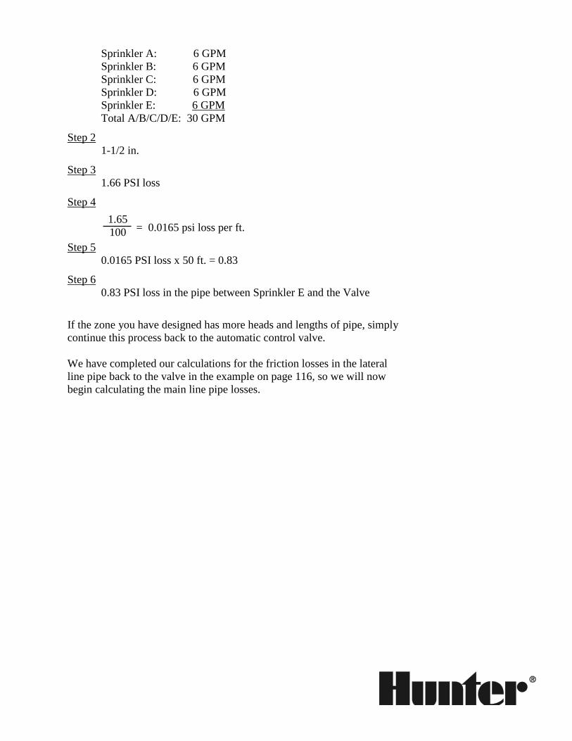
Sprinkler A: 6 GPM
Sprinkler B: 6 GPM
Sprinkler C: 6 GPM
Sprinkler D: 6 GPM
Sprinkler E: 6 GPM
Total A/B/C/D/E: 30 GPM
Step 2
1-1/2 in.
Step 3
1.66 PSI loss
Step 4
Step 5
0.0165 PSI loss x 50 ft. = 0.83
Step 6
0.83 PSI loss in the pipe between Sprinkler E and the Valve
If the zone you have designed has more heads and lengths of pipe, simply
continue this process back to the automatic control valve.
We have completed our calculations for the friction losses in the lateral
line pipe back to the valve in the example on page 116, so we will now
begin calculating the main line pipe losses.
1.65
100 = 0.0165 psi loss per ft.
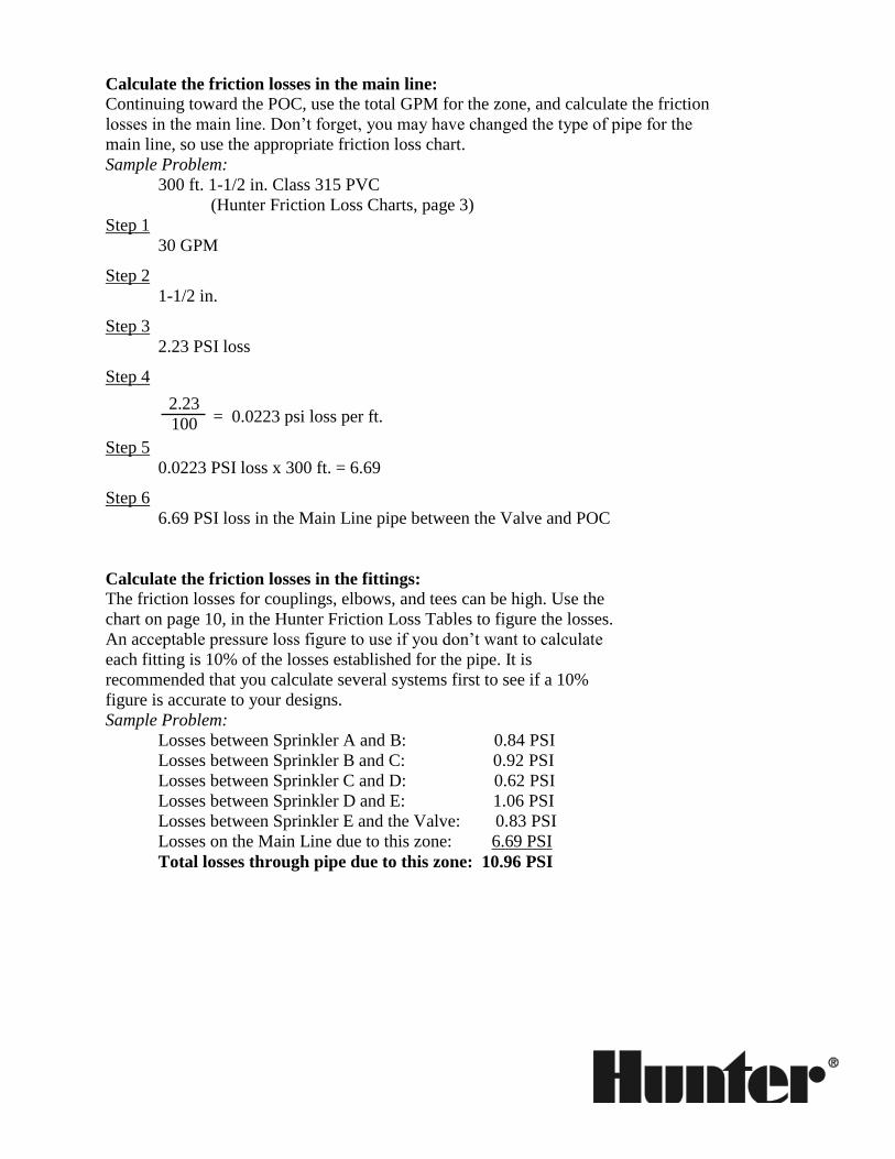
Calculate the friction losses in the main line:
Continuing toward the POC, use the total GPM for the zone, and calculate the friction
losses in the main line. Don’t forget, you may have changed the type of pipe for the
main line, so use the appropriate friction loss chart.
Sample Problem:
300 ft. 1-1/2 in. Class 315 PVC
(Hunter Friction Loss Charts, page 3)
Step 1
30 GPM
Step 2
1-1/2 in.
Step 3
2.23 PSI loss
Step 4
Step 5
0.0223 PSI loss x 300 ft. = 6.69
Step 6
6.69 PSI loss in the Main Line pipe between the Valve and POC
Calculate the friction losses in the fittings:
The friction losses for couplings, elbows, and tees can be high. Use the
chart on page 10, in the Hunter Friction Loss Tables to figure the losses.
An acceptable pressure loss figure to use if you don’t want to calculate
each fitting is 10% of the losses established for the pipe. It is
recommended that you calculate several systems first to see if a 10%
figure is accurate to your designs.
Sample Problem:
Losses between Sprinkler A and B: 0.84 PSI
Losses between Sprinkler B and C: 0.92 PSI
Losses between Sprinkler C and D: 0.62 PSI
Losses between Sprinkler D and E: 1.06 PSI
Losses between Sprinkler E and the Valve: 0.83 PSI
Losses on the Main Line due to this zone: 6.69 PSI
Total losses through pipe due to this zone: 10.96 PSI
2.23
100 = 0.0223 psi loss per ft.
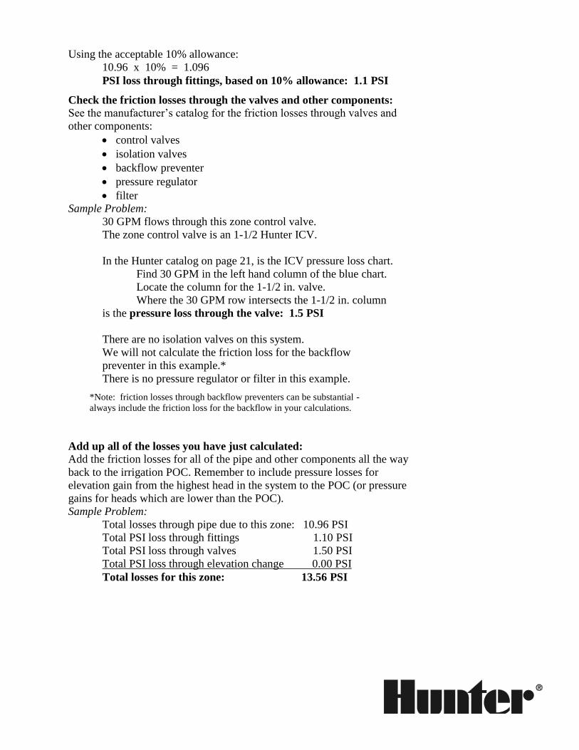
Using the acceptable 10% allowance:
10.96 x 10% = 1.096
PSI loss through fittings, based on 10% allowance: 1.1 PSI
Check the friction losses through the valves and other components:
See the manufacturer’s catalog for the friction losses through valves and
other components:
control valves
isolation valves
backflow preventer
pressure regulator
filter
Sample Problem:
30 GPM flows through this zone control valve.
The zone control valve is an 1-1/2 Hunter ICV.
In the Hunter catalog on page 21, is the ICV pressure loss chart.
Find 30 GPM in the left hand column of the blue chart.
Locate the column for the 1-1/2 in. valve.
Where the 30 GPM row intersects the 1-1/2 in. column
is the pressure loss through the valve: 1.5 PSI
There are no isolation valves on this system.
We will not calculate the friction loss for the backflow
preventer in this example.*
There is no pressure regulator or filter in this example.
*Note: friction losses through backflow preventers can be substantial -
always include the friction loss for the backflow in your calculations.
Add up all of the losses you have just calculated: Add the friction losses for all of the pipe and other components all the way
back to the irrigation POC. Remember to include pressure losses for
elevation gain from the highest head in the system to the POC (or pressure
gains for heads which are lower than the POC).
Sample Problem:
Total losses through pipe due to this zone: 10.96 PSI
Total PSI loss through fittings 1.10 PSI
Total PSI loss through valves 1.50 PSI
Total PSI loss through elevation change 0.00 PSI
Total losses for this zone: 13.56 PSI

Check to be sure that the PSI losses do not exceed the available PSI
for the system. Refer back to the original calculation for design capacity and dynamic
pressure. Make sure the system requirements that you just added up are
within the calculated design capacity. Subtract the system’s friction loss
from the dynamic pressure at design capacity at the POC (line #20 on the
Design Capacity worksheet for metered and unmetered systems, line #17
for pump systems). Make sure the final dynamic pressure is sufficient to
operate the sprinklers chosen for the project.
Many designers will add the PSI requirement for the sprinkler to the total
PSI losses. (For instance: if the operating pressure for the head in our
example is 50 PSI, then you would add 50 PSI to the 13.56 PSI loss
calculated, for a total of 63.56 minimum PSI requirement.)
Total losses for this zone: 13.56 PSI
Operating pressure required for head 50.0 PSI
Minimum PSI requirement for system 63.56 PSI
If the dynamic pressure at design capacity at the POC (line #20 on the
Design Capacity worksheet) is 70 PSI, then you have sufficient pressure to
operate this system.
If however, the pressure on your Design Capacity worksheet is 60 PSI,
then you will need to resize the pipe, valves, and/or other components, or
reduce the number of heads in order to lower the friction losses through
the system.
Repeat this friction loss calculation process for each critical zone, and for
the critical zone(s) for each different type of sprinkler chosen.
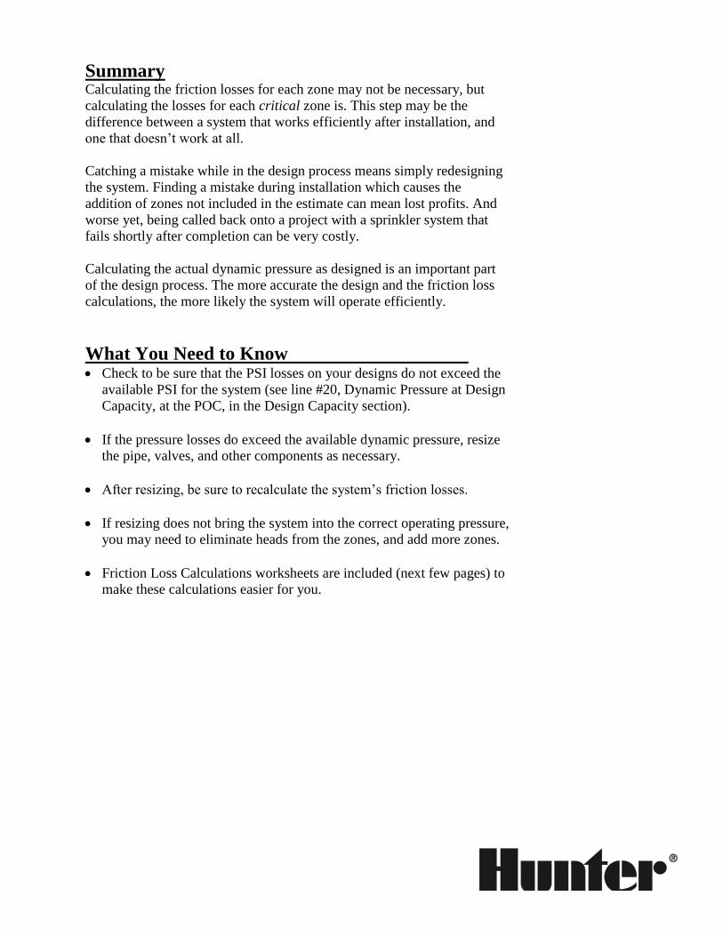
Summary
Calculating the friction losses for each zone may not be necessary, but
calculating the losses for each critical zone is. This step may be the
difference between a system that works efficiently after installation, and
one that doesn’t work at all.
Catching a mistake while in the design process means simply redesigning
the system. Finding a mistake during installation which causes the
addition of zones not included in the estimate can mean lost profits. And
worse yet, being called back onto a project with a sprinkler system that
fails shortly after completion can be very costly.
Calculating the actual dynamic pressure as designed is an important part
of the design process. The more accurate the design and the friction loss
calculations, the more likely the system will operate efficiently.
What You Need to Know
Check to be sure that the PSI losses on your designs do not exceed the
available PSI for the system (see line #20, Dynamic Pressure at Design
Capacity, at the POC, in the Design Capacity section).
If the pressure losses do exceed the available dynamic pressure, resize
the pipe, valves, and other components as necessary.
After resizing, be sure to recalculate the system’s friction losses.
If resizing does not bring the system into the correct operating pressure,
you may need to eliminate heads from the zones, and add more zones.
Friction Loss Calculations worksheets are included (next few pages) to
make these calculations easier for you.

Friction Loss Calculations
Type of
Pipe Size of
Size GPM Flow
Loss per 100 ft.
Loss per Foot
Length of Pipe
Loss per Length
Lateral Line
Lateral Line
Lateral Line
Lateral Line
Lateral Line
Lateral Line
Lateral Line
Lateral Line
Lateral Line
Lateral Line
Lateral Line
Lateral Line
Main Line
Main Line
Main Line
Zone GPM
Size PSI Loss
Subtotal Pressure Losses in Pipe (above)
Fittings - Subtotal of the Pressure Losses in Pipe __________ x 10%
Control Valve
Isolation Valve
Isolation Valve
Backflow Preventer
Pressure Regulator
Filter
Miscellaneous
Miscellaneous
Miscellaneous
Loss or (Gain) - Elevation
Project
Design Capacity
Dynamic Pressure (at Design Capacity, at the POC -
Line #20 on the Design Capacity Worksheet) Zone Number
Notes:
Total Pressure Loss
Pressure Required at the Head
Minimum Pressure Required for Sprinkler Operation as Designed
(Compare to Dynamic Pressure at Design Capacity at the POC, above)
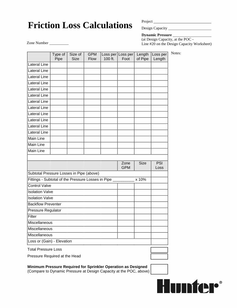
Precipitation Rates Introduction Today's irrigation designer or system manager faces a multitude of
concerns including:
• increased costs for water
• higher bills for pumping
• excessive runoff
• too much or too little water applied
• wet spots that do not allow use of a turf or landscape
• dry spots that are unsightly or cause lost plant material
• increased pests and diseases
Each of these concerns can be related to precipitation rates. Thus,
understanding precipitation rates can help you avoid these common
problems, leading to improved landscapes and reduced costs through
better irrigation design and management.
What Is “Precipitation Rate?” If someone said they were caught in a rainstorm that dropped one inch of
water in an hour you would have some idea of how “hard” or “heavily”
the rain came down. A rainstorm that covers an area with one inch of
water in one hour has a “precipitation rate” of one inch per hour (1 in./hr).
Similarly, if a sprinkler system applies enough water to cover the irrigated
area with one inch of water in one hour, the sprinkler system also has a
precipitation rate of 1 in./hr. Thus, the precipitation rate is the speed at
which a sprinkler or an irrigation system applies water.
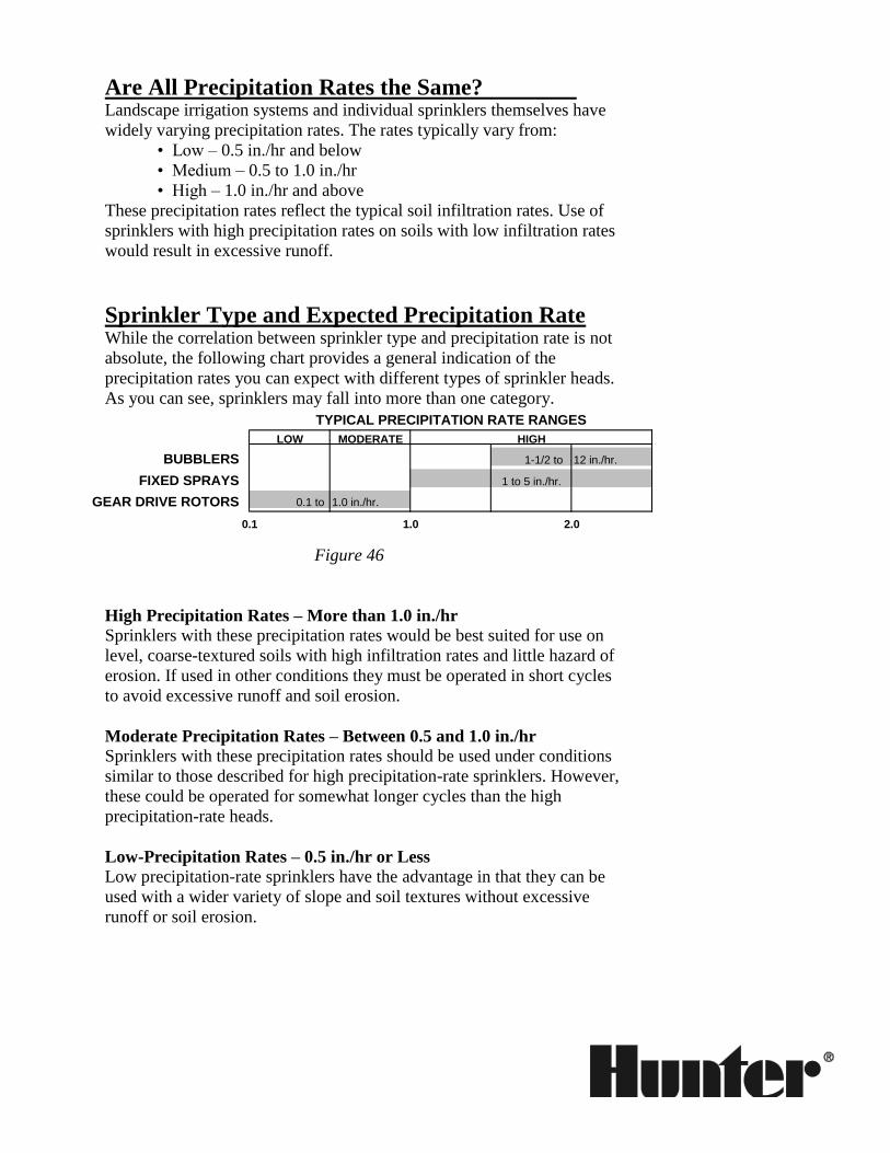
Are All Precipitation Rates the Same? Landscape irrigation systems and individual sprinklers themselves have
widely varying precipitation rates. The rates typically vary from:
• Low – 0.5 in./hr and below
• Medium – 0.5 to 1.0 in./hr
• High – 1.0 in./hr and above
These precipitation rates reflect the typical soil infiltration rates. Use of
sprinklers with high precipitation rates on soils with low infiltration rates
would result in excessive runoff.
Sprinkler Type and Expected Precipitation Rate While the correlation between sprinkler type and precipitation rate is not
absolute, the following chart provides a general indication of the
precipitation rates you can expect with different types of sprinkler heads.
As you can see, sprinklers may fall into more than one category.
TYPICAL PRECIPITATION RATE RANGES
LOW MODERATE HIGH
BUBBLERS 1-1/2 to 12 in./hr.
FIXED SPRAYS 1 to 5 in./hr.
GEAR DRIVE ROTORS 0.1 to 1.0 in./hr.
0.1 1.0 2.0
Figure 46
High Precipitation Rates – More than 1.0 in./hr
Sprinklers with these precipitation rates would be best suited for use on
level, coarse-textured soils with high infiltration rates and little hazard of
erosion. If used in other conditions they must be operated in short cycles
to avoid excessive runoff and soil erosion.
Moderate Precipitation Rates – Between 0.5 and 1.0 in./hr
Sprinklers with these precipitation rates should be used under conditions
similar to those described for high precipitation-rate sprinklers. However,
these could be operated for somewhat longer cycles than the high
precipitation-rate heads.
Low-Precipitation Rates – 0.5 in./hr or Less
Low precipitation-rate sprinklers have the advantage in that they can be
used with a wider variety of slope and soil textures without excessive
runoff or soil erosion.
Sprinkler Precipitation Rates
Versus System Precipitation Rates Depending on the construction of the irrigation system, the precipitation
rate may be quoted as either a “sprinkler” or a “system” rate.
The precipitation rate of a system is inversely related to head spacing and
row spacing. With the sprinkler flow rate remaining the same, increasing
head or row spacing decreases the precipitation rate while reducing head
or row spacing increases the precipitation rate.
Sprinkler Precipitation Rates The precipitation rate for a “sprinkler” refers to the rate for a system in
which only one specific type of head and nozzle is used. The precipitation
rate for a single sprinkler is calculated using the Sprinkler Spacing
Method. This method calculates the precipitation rate for those sprinkler
heads with the same spacing, rate of flow (in gallons per minute, or GPM)
and arc of spray.
System Precipitation Rates The precipitation rate for a “system” is the average precipitation rate of all
sprinklers in an area regardless of the arc, spacing, or flow rate for each
head. The system precipitation rate is calculated using the Total Area
Method. The area for which the calculation is made usually corresponds
to all the heads on one irrigation control valve, but can include many
valves in an area. While individual heads in an area may have different
precipitation rates, this method gives you an average over the entire area.
The Total Area Method is most useful and accurate when all the heads in
the area have similar precipitation rates. Where the precipitation rates of
the sprinkler heads vary considerably, the average precipitation rate can be
misleading. Where there are differences in precipitation rates, the
irrigation system may have applied enough water to the “average” area,
but there very likely will be dry spots and wet spots as well.
Note: It is important to remember that precipitation rates and
system uniformity are two completely separate issues. Calculated
precipitation rates do not reflect how uniformly the water is being
applied. System uniformity is an important variable and should
always be taken into account when scheduling irrigation systems
or determining minimum water supply requirements.
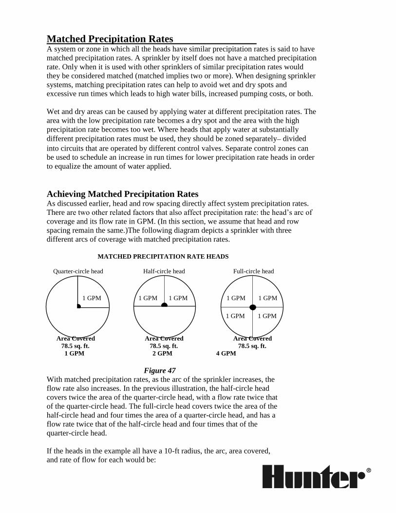
Matched Precipitation Rates A system or zone in which all the heads have similar precipitation rates is said to have
matched precipitation rates. A sprinkler by itself does not have a matched precipitation
rate. Only when it is used with other sprinklers of similar precipitation rates would
they be considered matched (matched implies two or more). When designing sprinkler
systems, matching precipitation rates can help to avoid wet and dry spots and
excessive run times which leads to high water bills, increased pumping costs, or both.
Wet and dry areas can be caused by applying water at different precipitation rates. The
area with the low precipitation rate becomes a dry spot and the area with the high
precipitation rate becomes too wet. Where heads that apply water at substantially
different precipitation rates must be used, they should be zoned separately– divided
into circuits that are operated by different control valves. Separate control zones can
be used to schedule an increase in run times for lower precipitation rate heads in order
to equalize the amount of water applied.
Achieving Matched Precipitation Rates As discussed earlier, head and row spacing directly affect system precipitation rates.
There are two other related factors that also affect precipitation rate: the head’s arc of
coverage and its flow rate in GPM. (In this section, we assume that head and row
spacing remain the same.)The following diagram depicts a sprinkler with three
different arcs of coverage with matched precipitation rates.
MATCHED PRECIPITATION RATE HEADS
Quarter-circle head Half-circle head Full-circle head
1 GPM 1 GPM 1 GPM 1 GPM 1 GPM
1 GPM 1 GPM
Area Covered Area Covered Area Covered
78.5 sq. ft. 78.5 sq. ft. 78.5 sq. ft.
1 GPM 2 GPM 4 GPM
Figure 47 With matched precipitation rates, as the arc of the sprinkler increases, the
flow rate also increases. In the previous illustration, the half-circle head
covers twice the area of the quarter-circle head, with a flow rate twice that
of the quarter-circle head. The full-circle head covers twice the area of the
half-circle head and four times the area of a quarter-circle head, and has a
flow rate twice that of the half-circle head and four times that of the
quarter-circle head.
If the heads in the example all have a 10-ft radius, the arc, area covered,
and rate of flow for each would be:
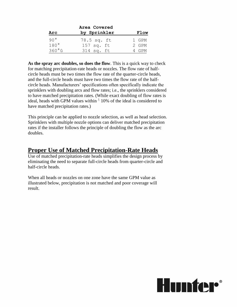
Area Covered
Arc by Sprinkler Flow
90° 78.5 sq. ft 1 GPM
180° 157 sq. ft 2 GPM
360°û 314 sq. ft 4 GPM
As the spray arc doubles, so does the flow. This is a quick way to check
for matching precipitation-rate heads or nozzles. The flow rate of half-
circle heads must be two times the flow rate of the quarter-circle heads,
and the full-circle heads must have two times the flow rate of the half-
circle heads. Manufacturers’ specifications often specifically indicate the
sprinklers with doubling arcs and flow rates; i.e., the sprinklers considered
to have matched precipitation rates. (While exact doubling of flow rates is
ideal, heads with GPM values within + 10% of the ideal is considered to
have matched precipitation rates.)
This principle can be applied to nozzle selection, as well as head selection.
Sprinklers with multiple nozzle options can deliver matched precipitation
rates if the installer follows the principle of doubling the flow as the arc
doubles.
Proper Use of Matched Precipitation-Rate Heads Use of matched precipitation-rate heads simplifies the design process by
eliminating the need to separate full-circle heads from quarter-circle and
half-circle heads.
When all heads or nozzles on one zone have the same GPM value as
illustrated below, precipitation is not matched and poor coverage will
result.
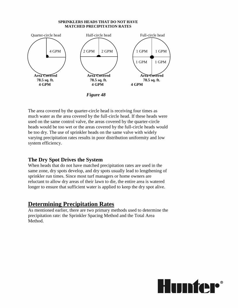
SPRINKLERS HEADS THAT DO NOT HAVE
MATCHED PRECIPITATION RATES
Quarter-circle head Half-circle head Full-circle head
4 GPM 2 GPM 2 GPM 1 GPM 1 GPM
1 GPM 1 GPM
Area Covered Area Covered Area Covered
78.5 sq. ft. 78.5 sq. ft. 78.5 sq. ft.
4 GPM 4 GPM 4 GPM
Figure 48
The area covered by the quarter-circle head is receiving four times as
much water as the area covered by the full-circle head. If these heads were
used on the same control valve, the areas covered by the quarter-circle
heads would be too wet or the areas covered by the full-circle heads would
be too dry. The use of sprinkler heads on the same valve with widely
varying precipitation rates results in poor distribution uniformity and low
system efficiency.
The Dry Spot Drives the System When heads that do not have matched precipitation rates are used in the
same zone, dry spots develop, and dry spots usually lead to lengthening of
sprinkler run times. Since most turf managers or home owners are
reluctant to allow dry areas of their lawn to die, the entire area is watered
longer to ensure that sufficient water is applied to keep the dry spot alive.
Determining Precipitation Rates As mentioned earlier, there are two primary methods used to determine the
precipitation rate: the Sprinkler Spacing Method and the Total Area
Method.
The Sprinkler Spacing Method This method is used to determine the precipitation rate for a single
sprinkler. The rate is calculated assuming the sprinkler is used in
conjunction with other sprinklers of the same kind (i.e., same arc, flow,
and spacing). With this method, one can compare the precipitation rate of
similar types of sprinkler heads with each other.
The following Sprinkler Spacing Method formula is applicable to heads of
any arc.
Pr = 34650 x GPM (for any arc)
Degrees of Arc x Head Spacing x Row
Spacing
Where:
Pr is the precipitation rate in inches per hour.
34650 is a constant that converts gallons per minute to inches per
hour for sprinklers with any arc. It is derived from 60 min/hr
divided by 7.48 gallons per cu ft, multiplied by 12 in. per ft times
360 degrees. (Note: If the flow of the head is in gallons per hour
(GPH), instead of gallons per minute (GPM), the constant should be
changed to 577.5).
GPM is the rated flow of the head used, regardless of its arc, in
gallons per minute.
Degrees of Arc is the arc of the spray pattern, in degrees, for
the sprinkler selected (full circle = 360°, half circle = 180°, etc.).
Head Spacing is the distance in feet between heads in the same
row.
Row Spacing is the distance in feet between the rows of
sprinklers.
While this information is helpful when comparing the precipitation rate of
similar types of sprinkler heads with each other, extreme caution should be
exercised when using the manufacturer’s
published precipitation rate information for a single sprinkler.
1. Often these are calculated for different degrees of arc (e.g.
360° vs. 180°) from manufacturer to manufacturer.
2. The manufacturer’s stated precipitation rate is calculated at an
exact pressure and spacing. Most layouts have specific
conditions that are different from one job to another.
We recommend you always calculate the precipitation rate for your
situation using the Total Area Method.
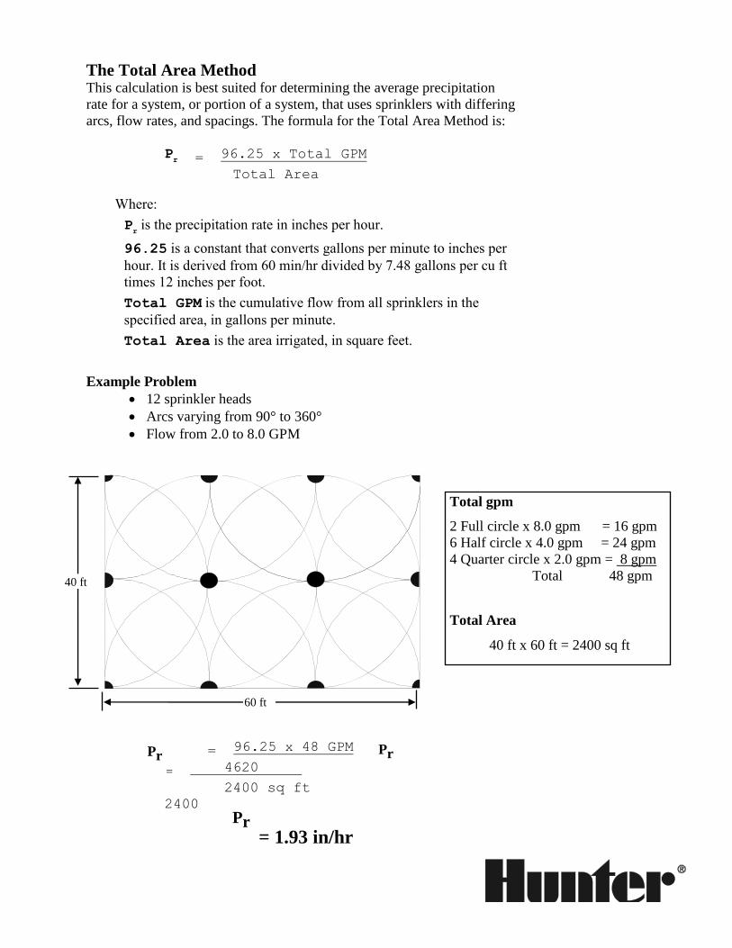
The Total Area Method This calculation is best suited for determining the average precipitation
rate for a system, or portion of a system, that uses sprinklers with differing
arcs, flow rates, and spacings. The formula for the Total Area Method is:
Pr = 96.25 x Total GPM
Total Area
Where:
Pr is the precipitation rate in inches per hour.
96.25 is a constant that converts gallons per minute to inches per
hour. It is derived from 60 min/hr divided by 7.48 gallons per cu ft
times 12 inches per foot.
Total GPM is the cumulative flow from all sprinklers in the
specified area, in gallons per minute.
Total Area is the area irrigated, in square feet.
Example Problem
12 sprinkler heads
Arcs varying from 90° to 360°
Flow from 2.0 to 8.0 GPM
= 96.25 x 48 GPM =
= 4620
2400 sq ft
2400
= 1.93 in/hr
Pr Pr Pr
Pr
Total gpm
2 Full circle x 8.0 gpm = 16 gpm
6 Half circle x 4.0 gpm = 24 gpm
4 Quarter circle x 2.0 gpm = 8 gpm
Total 48 gpm
Total Area
40 ft x 60 ft = 2400 sq ft
60 ft
40 ft
Use of Precipitation Rates in Landscape Irrigation Precipitation rate is critical to the selection of sprinkler heads for a system
and scheduling sprinkler run times.
When selecting sprinkler heads, it is necessary to limit the amount of
water applied to the infiltration rate of the soil. The infiltration rate is
affected by the soil texture, soil structure, plant material, and the slope.
Failure to limit the amount of water applied to the infiltration rate of the
soil can result in excessive runoff and erosion. Matching the amount of
water applied to the soil’s infiltration rate can be done either by selecting a
sprinkler according to its precipitation rate or by scheduling the sprinkler
system’s run time.
This concept will be further discussed in the section on Irrigation
Scheduling.
Precipitation Rate versus Sprinkler Run Time. As previously stated,
the amount of time required to irrigate a project is not typically affected by
the sprinkler precipitation rate. While it is true that lower precipitation rate
heads must be run for a longer periods of time, more heads can be
installed on a zone and, therefore, the total irrigation time for an entire
project will be the same for high precipitation-rate heads with many zones,
and low precipitation-rate heads with few zones.
Similar run times can be confirmed by checking the design capacity. If
designs with both high and low precipitation-rate heads use the maximum
flow rate available for the project (design capacity) then both projects will
have similar total run times.
Summary
Scheduling sprinkler run times without knowing the precipitation rate is
like trying to estimate your arrival time without knowing how fast you are
traveling. The precipitation rate represents the speed at which an amount
of water is applied. Knowing this is important because it helps us estimate
how long it will take to apply the water needed by the plants in the
landscape. The precipitation rate is also required for proper irrigation
scheduling to prevent dry or wet areas. If the precipitation rate is not
known, the tendency is to over water to be sure enough water is applied.

What You Need to Know
Precipitation rate, measured in inches per hour (in./hr.), is the speed at
which a sprinkler or an irrigation system applies water.
Matched precipitation means that all of the sprinklers on one zone have
similar precipitation rates. In other words, as the arc of a sprinkler
increases, the flow should increase proportionally.
The formula for determining the precipitation rate for a given area is:
Pr = 96.25 x Total GPM
Total Area
Irrigation Scheduling Introduction Ultimately, the goal of the landscape manager is to apply only the amount
of water needed, and to apply that water only when it is needed. Plants
have an effective root zone (RZ), and water in the soil below that root
zone is unusable by the plants. The effective root zone for turf grass, for
instance, is about six inches to a foot deep.
A basic truth of plant irrigation is this: Irrigation is not meant to water the
plants; rather, it is meant to refill the reservoir from which those plants
will draw the water they need. If the reservoir gets too “empty,” the plants
begin to wilt. When they are deprived of water for too long, a “permanent
wilting point” is reached, and permanent plant damage occurs.
If the reservoir is allowed to get “too full,” the soil may reach “field
capacity” at levels below the plant’s effective root zone, and water would
go unused. Field capacity is the upper limit of storable water in a layer of
soil after the water has drained through.
It might seem that a slow and constant supply of water would be the best
way to fulfill the watering requirement. However, in most circumstances,
daily watering is wasteful. Water evaporates quite rapidly from the top
few inches of soil; the rate of evaporation can reach as much as 50% per
day. The deeper the moisture level in the soil, the lower the daily
evaporation rate.
It becomes important then, to manage the amount of water in the root zone
to maximize application efficiency. When scheduling irrigation, provide
enough water, at the proper times to keep the moisture level at the root
zone between the permanent wilting point, and the field capacity.
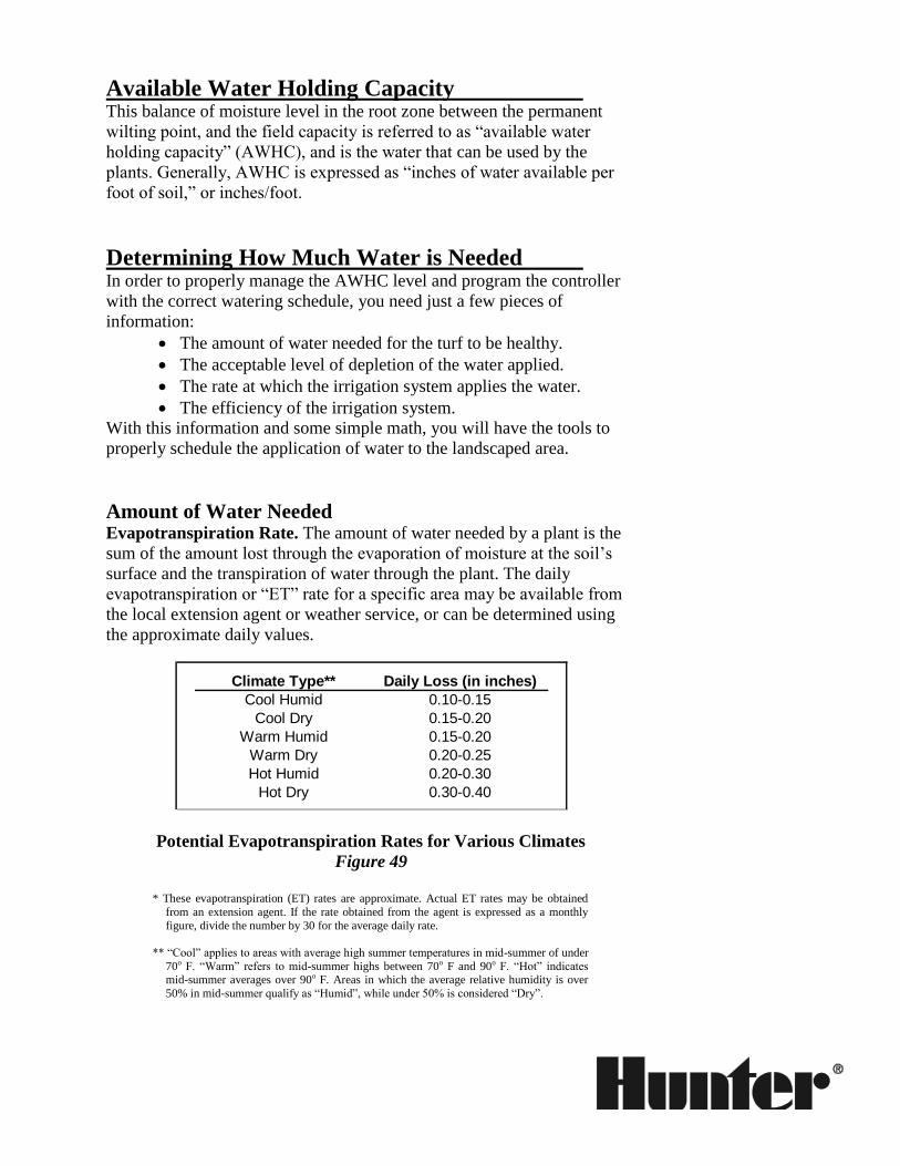
Available Water Holding Capacity This balance of moisture level in the root zone between the permanent
wilting point, and the field capacity is referred to as “available water
holding capacity” (AWHC), and is the water that can be used by the
plants. Generally, AWHC is expressed as “inches of water available per
foot of soil,” or inches/foot.
Determining How Much Water is Needed
In order to properly manage the AWHC level and program the controller
with the correct watering schedule, you need just a few pieces of
information:
The amount of water needed for the turf to be healthy.
The acceptable level of depletion of the water applied.
The rate at which the irrigation system applies the water.
The efficiency of the irrigation system.
With this information and some simple math, you will have the tools to
properly schedule the application of water to the landscaped area.
Amount of Water Needed Evapotranspiration Rate. The amount of water needed by a plant is the
sum of the amount lost through the evaporation of moisture at the soil’s
surface and the transpiration of water through the plant. The daily
evapotranspiration or “ET” rate for a specific area may be available from
the local extension agent or weather service, or can be determined using
the approximate daily values.
Climate Type** Daily Loss (in inches)
Cool Humid 0.10-0.15
Cool Dry 0.15-0.20
Warm Humid 0.15-0.20
Warm Dry 0.20-0.25
Hot Humid 0.20-0.30
Hot Dry 0.30-0.40
Potential Evapotranspiration Rates for Various Climates
Figure 49
* These evapotranspiration (ET) rates are approximate. Actual ET rates may be obtained
from an extension agent. If the rate obtained from the agent is expressed as a monthly
figure, divide the number by 30 for the average daily rate.
** “Cool” applies to areas with average high summer temperatures in mid-summer of under
70o F. “Warm” refers to mid-summer highs between 70o F and 90o F. “Hot” indicates mid-summer averages over 90o F. Areas in which the average relative humidity is over
50% in mid-summer qualify as “Humid”, while under 50% is considered “Dry”.
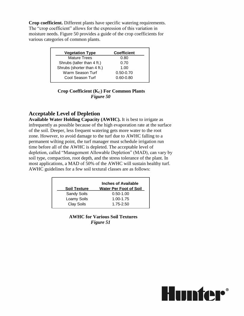
Crop coefficient. Different plants have specific watering requirements.
The “crop coefficient” allows for the expression of this variation in
moisture needs. Figure 50 provides a guide of the crop coefficients for
various categories of common plants.
Vegetation Type Coefficient
Mature Trees 0.80
Shrubs (taller than 4 ft.) 0.70
Shrubs (shorter than 4 ft.) 1.00
Warm Season Turf 0.50-0.70
Cool Season Turf 0.60-0.80
Crop Coefficient (KC) For Common Plants
Figure 50
Acceptable Level of Depletion Available Water Holding Capacity (AWHC). It is best to irrigate as
infrequently as possible because of the high evaporation rate at the surface
of the soil. Deeper, less frequent watering gets more water to the root
zone. However, to avoid damage to the turf due to AWHC falling to a
permanent wilting point, the turf manager must schedule irrigation run
time before all of the AWHC is depleted. The acceptable level of
depletion, called “Management Allowable Depletion” (MAD), can vary by
soil type, compaction, root depth, and the stress tolerance of the plant. In
most applications, a MAD of 50% of the AWHC will sustain healthy turf.
AWHC guidelines for a few soil textural classes are as follows:
Inches of Available
Soil Texture Water Per Foot of Soil
Sandy Soils 0.50-1.00
Loamy Soils 1.00-1.75
Clay Soils 1.75-2.50
AWHC for Various Soil Textures
Figure 51
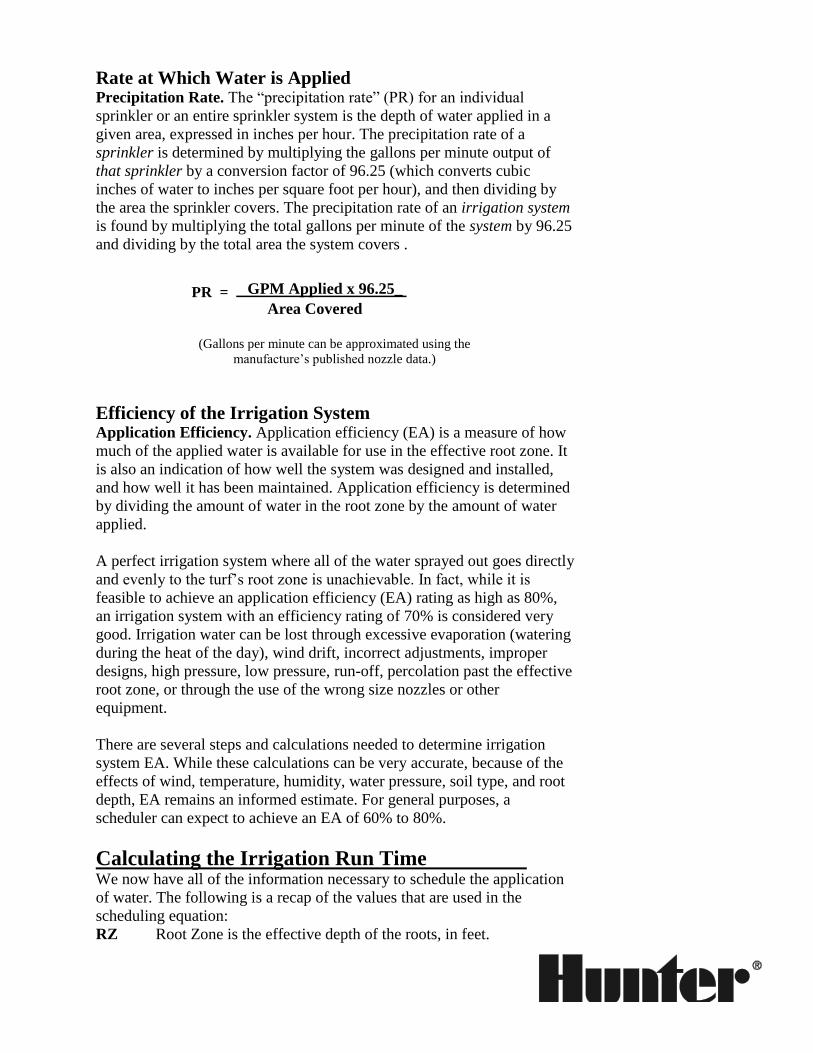
Rate at Which Water is Applied
Precipitation Rate. The “precipitation rate” (PR) for an individual
sprinkler or an entire sprinkler system is the depth of water applied in a
given area, expressed in inches per hour. The precipitation rate of a
sprinkler is determined by multiplying the gallons per minute output of
that sprinkler by a conversion factor of 96.25 (which converts cubic
inches of water to inches per square foot per hour), and then dividing by
the area the sprinkler covers. The precipitation rate of an irrigation system
is found by multiplying the total gallons per minute of the system by 96.25
and dividing by the total area the system covers .
PR = GPM Applied x 96.25_
Area Covered
(Gallons per minute can be approximated using the
manufacture’s published nozzle data.)
Efficiency of the Irrigation System
Application Efficiency. Application efficiency (EA) is a measure of how
much of the applied water is available for use in the effective root zone. It
is also an indication of how well the system was designed and installed,
and how well it has been maintained. Application efficiency is determined
by dividing the amount of water in the root zone by the amount of water
applied.
A perfect irrigation system where all of the water sprayed out goes directly
and evenly to the turf’s root zone is unachievable. In fact, while it is
feasible to achieve an application efficiency (EA) rating as high as 80%,
an irrigation system with an efficiency rating of 70% is considered very
good. Irrigation water can be lost through excessive evaporation (watering
during the heat of the day), wind drift, incorrect adjustments, improper
designs, high pressure, low pressure, run-off, percolation past the effective
root zone, or through the use of the wrong size nozzles or other
equipment.
There are several steps and calculations needed to determine irrigation
system EA. While these calculations can be very accurate, because of the
effects of wind, temperature, humidity, water pressure, soil type, and root
depth, EA remains an informed estimate. For general purposes, a
scheduler can expect to achieve an EA of 60% to 80%.
Calculating the Irrigation Run Time We now have all of the information necessary to schedule the application
of water. The following is a recap of the values that are used in the
scheduling equation:
RZ Root Zone is the effective depth of the roots, in feet.
ET Evaporation of soil surface water plus Transpiration of water
through the plant. (Figure 49)
KC Crop coefficient is the specific water requirement of the plant.
(Figure 50)
AWHC Available Water Holding Capacity is the moisture level in
the soil (expressed in inches per foot) which is above the plant’s
permanent wilting point, and below the soil’s field capacity. (Figure 51)
MAD Management Allowable Depletion of water from the
AWHC. (In most applications, a MAD of 50% will sustain a
healthy landscape.)
PR Precipitation Rate is the depth of water per unit of time.
(Multiply the total gallons per minute of the system by 96.25
and divide by the total area the system covers.)
EA Application Efficiency is a measure of the overall efficiency
of the sprinkler system. (60% to 80%)
The frequency (F), or “Set Days To Water”, is calculated using the
following formula:
F = AWHC x RZ x MAD
ET x KC
The amount of run time (RT) or “Set Station Run Times” each watering is
calculated:
RT = 60 x F x ET x KC
PR x EA
Example: A valve in your system is irrigating established warm season
turf which is growing in a sandy loam on a slight slope. The average
precipitation rate is 0.49 inches/hour. The system is located in San
Marcos, CA, where the daily moisture loss (ET) to be replenished is 0.20
inches. The system application efficiency is approximately 65%.
Answer:
Watering Frequency
F = 1.0” x 0.75” x 50% = 1.0 x 0.75 x 0.50 = 0.375 = 2.68
0.20 x 0.70 0.20 x 0.70 0.14
The answer is a 2 or 3 day watering interval. The scheduler may decide to
use a 3 day interval (water on day #1, wait day #2 and day #3, and then
begin the watering interval again on the next day), and monitor the turf’s
condition.
Run Time per Frequency
RT = 60 x 3 x 0.20 x 0.70 = 180 x 0.14 = 25.2 = 79
0.49 x 65% 0.49 x 0.65 0.319
Water 79 minutes each watering.
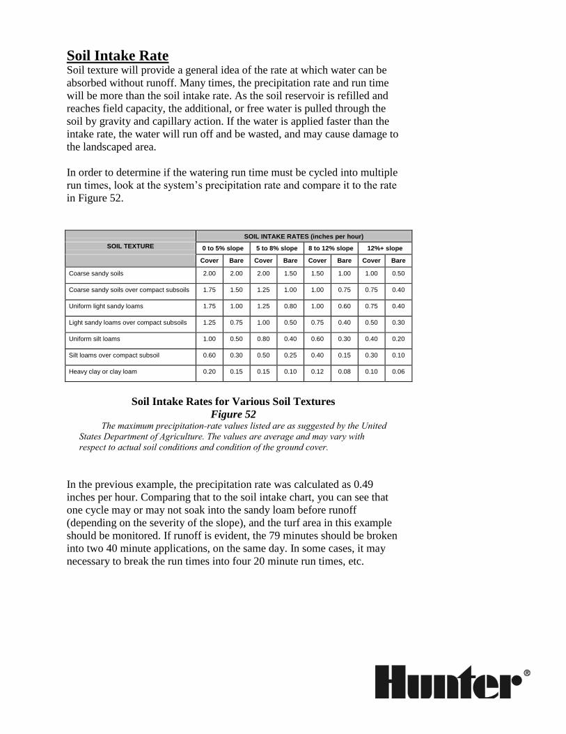
Soil Intake Rate
Soil texture will provide a general idea of the rate at which water can be
absorbed without runoff. Many times, the precipitation rate and run time
will be more than the soil intake rate. As the soil reservoir is refilled and
reaches field capacity, the additional, or free water is pulled through the
soil by gravity and capillary action. If the water is applied faster than the
intake rate, the water will run off and be wasted, and may cause damage to
the landscaped area.
In order to determine if the watering run time must be cycled into multiple
run times, look at the system’s precipitation rate and compare it to the rate
in Figure 52.
SOIL INTAKE RATES (inches per hour)
SOIL TEXTURE
0 to 5% slope
5 to 8% slope
8 to 12% slope
12%+ slope
Cover
Bare
Cover
Bare
Cover
Bare
Cover
Bare
Coarse sandy soils
2.00
2.00
2.00
1.50
1.50
1.00
1.00
0.50
Coarse sandy soils over compact subsoils
1.75
1.50
1.25
1.00
1.00
0.75
0.75
0.40
Uniform light sandy loams
1.75
1.00
1.25
0.80
1.00
0.60
0.75
0.40
Light sandy loams over compact subsoils
1.25
0.75
1.00
0.50
0.75
0.40
0.50
0.30
Uniform silt loams
1.00
0.50
0.80
0.40
0.60
0.30
0.40
0.20
Silt loams over compact subsoil
0.60
0.30
0.50
0.25
0.40
0.15
0.30
0.10
Heavy clay or clay loam
0.20
0.15
0.15
0.10
0.12
0.08
0.10
0.06
Soil Intake Rates for Various Soil Textures
Figure 52 The maximum precipitation-rate values listed are as suggested by the United
States Department of Agriculture. The values are average and may vary with
respect to actual soil conditions and condition of the ground cover.
In the previous example, the precipitation rate was calculated as 0.49
inches per hour. Comparing that to the soil intake chart, you can see that
one cycle may or may not soak into the sandy loam before runoff
(depending on the severity of the slope), and the turf area in this example
should be monitored. If runoff is evident, the 79 minutes should be broken
into two 40 minute applications, on the same day. In some cases, it may
necessary to break the run times into four 20 minute run times, etc.
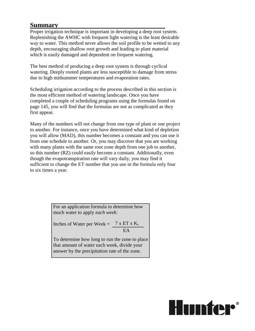
Summary
Proper irrigation technique is important in developing a deep root system.
Replenishing the AWHC with frequent light watering is the least desirable
way to water. This method never allows the soil profile to be wetted to any
depth, encouraging shallow root growth and leading to plant material
which is easily damaged and dependent on frequent watering.
The best method of producing a deep root system is through cyclical
watering. Deeply rooted plants are less susceptible to damage from stress
due to high midsummer temperatures and evaporation rates.
Scheduling irrigation according to the process described in this section is
the most efficient method of watering landscape. Once you have
completed a couple of scheduling programs using the formulas found on
page 145, you will find that the formulas are not as complicated as they
first appear.
Many of the numbers will not change from one type of plant or one project
to another. For instance, once you have determined what kind of depletion
you will allow (MAD), this number becomes a constant and you can use it
from one schedule to another. Or, you may discover that you are working
with many plants with the same root zone depth from one job to another,
so this number (RZ) could easily become a constant. Additionally, even
though the evapotranspiration rate will vary daily, you may find it
sufficient to change the ET number that you use in the formula only four
to six times a year.
For an application formula to determine how
much water to apply each week:
Inches of Water per Week =
To determine how long to run the zone to place
that amount of water each week, divide your
answer by the precipitation rate of the zone.
7 x ET x Kc
EA
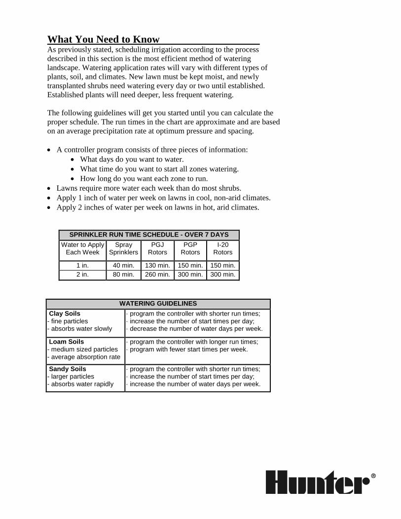
What You Need to Know
As previously stated, scheduling irrigation according to the process
described in this section is the most efficient method of watering
landscape. Watering application rates will vary with different types of
plants, soil, and climates. New lawn must be kept moist, and newly
transplanted shrubs need watering every day or two until established.
Established plants will need deeper, less frequent watering.
The following guidelines will get you started until you can calculate the
proper schedule. The run times in the chart are approximate and are based
on an average precipitation rate at optimum pressure and spacing.
A controller program consists of three pieces of information:
What days do you want to water.
What time do you want to start all zones watering.
How long do you want each zone to run.
Lawns require more water each week than do most shrubs.
Apply 1 inch of water per week on lawns in cool, non-arid climates.
Apply 2 inches of water per week on lawns in hot, arid climates.
SPRINKLER RUN TIME SCHEDULE - OVER 7 DAYS
Water to Apply Each Week
Spray Sprinklers
PGJ Rotors
PGP Rotors
I-20 Rotors
1 in. 40 min. 130 min. 150 min. 150 min.
2 in. 80 min. 260 min. 300 min. 300 min.
WATERING GUIDELINES
Clay Soils - fine particles - absorbs water slowly
· program the controller with shorter run times; · increase the number of start times per day; · decrease the number of water days per week.
Loam Soils - medium sized particles - average absorption rate
· program the controller with longer run times; · program with fewer start times per week.
Sandy Soils - larger particles - absorbs water rapidly
· program the controller with shorter run times; · increase the number of start times per day; · increase the number of water days per week.