Hungr 2010 - Manual de Clara-w
99
USER’S MANUAL CLARA-W SLOPE STABILITY ANALYSIS IN TWO OR THREE DIMENSIONS FOR MICROCOMPUTERS O.Hungr Geotechnical Research Inc. 4195 Almondel Road, West Vancouver B.C., Canada, V7V 3L6 Tel. (604) 926-9129 © O. Hungr Geotechnical Research Inc. March 2010 All rights reserved
-
Upload
kevin-mendoza -
Category
Documents
-
view
215 -
download
1
description
GEOTECNIA
Transcript of Hungr 2010 - Manual de Clara-w

USER’S MANUAL
CLARA-W
SLOPE STABILITY ANALYSIS IN TWO OR THREE DIMENSIONS FOR MICROCOMPUTERS
O.Hungr Geotechnical Research Inc. 4195 Almondel Road, West Vancouver
B.C., Canada, V7V 3L6 Tel. (604) 926-9129
© O. Hungr Geotechnical Research Inc. March 2010 All rights reserved

i
TABLE OF CONTENTS
PART A - DESCRIPTION OF THE PROGRAM AND ITS FUNCTIONS......................1
A.1 INTRODUCTION....................................................................................................2 A.1.1 Purpose...................................................................................................................2 A.1.2 Solution Algorithms...............................................................................................2 A.1.3 Typical Applications..............................................................................................3 A.1.4 Copyright and Licensing........................................................................................3 A.1.5 Precautions.............................................................................................................3 A.1.6 How to Use This Manual .......................................................................................5 A.1.7 List of Program Features........................................................................................5 A.1.8 Problem Size Limits...............................................................................................6
A.2 INPUT DATA ORGANIZATION..............................................................................7
A.2.1 Data Files ...............................................................................................................7 A.2.2 Coordinate System.................................................................................................7 A.2.3 Column Assembly (“Mesh”)..................................................................................7 A.2.4 Types of Surfaces: Cross-section-Based, Digital and At-Constant-Depth ............9 A.2.5 Input Cross-Sections ..............................................................................................9 A.2.6 Interpolation Methods..........................................................................................10 A.2.7 Sliding Surfaces ...................................................................................................13 A.2.8 Hard Layer Option ...............................................................................................17 A.2.9 Tension Cracks ....................................................................................................17 A.2.10 Two-Dimensional Configuration ........................................................................17 A.2.11 Material Properties..............................................................................................19 A.2.12 Discontinuities ....................................................................................................20 A.2.13 Piezometric Conditions .......................................................................................20 A.2.14 Toe Submergence................................................................................................22 A.2.15 External Loads ....................................................................................................22
A.3 PROGRAM CONTROL ...........................................................................................24
A.3.1 The Main Menu ...................................................................................................24 A.3.2 Input Screens........................................................................................................29 A.3.3 Error/warning Messages ......................................................................................29
PART B - DATA INPUT AND MANAGEMENT ..............................................................31
B.1 STARTING THE PROGRAM .................................................................................32 B.1.1 General.................................................................................................................32 B.1.2 Opening and Saving a Data File ..........................................................................32
B.2 CREATING AN INPUT DATA FILE .....................................................................34
ii
B.2.1 Data Preparation ..................................................................................................34 B.2.2 New File Sequence................................................................................................36 B.2.3 Control Parametres Screen...................................................................................36 B.2.4 Interpolation Method Screen ...............................................................................39 B.2.5 Material Properties Screen...................................................................................39 B.2.6 Discontinuity Properties ......................................................................................41 B.2.7 Stratigraphic Layer Surfaces Screen....................................................................41 B.2.8 Piezometric Surfaces Screen................................................................................42 B.2.9 Cross-section Positions screen.............................................................................42
B.3 GEOMETRY INPUT..................................................................................................43
B.3.1 Edit Cross-sections Screen...................................................................................43 B.3.2 Rules of Geometry Input......................................................................................44 B.3.3 How to Input/Edit Cross-Section Geometry........................................................45 B.3.4 Load and Scale Image Feature.............................................................................47 B.3.5 Using Digital Elevation Model (*.GRD) Files ....................................................48
PART C - SLOPE STABILITY ANALYSIS ......................................................................50
C.1 ANALYSIS OPTIONS ..............................................................................................51 C.1.1 General.................................................................................................................51 C.1.2 Earthquake Acceleration......................................................................................51 C.1.3 External Forces Screen ........................................................................................51 C.1.4 Tension Crack Screen ..........................................................................................51 C.1.5 Rotation of the Reference Frame ........................................................................53
C.2 DEFINITION OF SLIDING SURFACES AND SEARCHES...............................52
C.2.1 Input of a Single Ellipsoidal Sliding Surface.......................................................52 C.2.2 Grid Search For the Critical Ellipsoid-Description .............................................53 C.2.3 How to Input a Grid Search .................................................................................54 C.2.4 Automatic Search For the Critical Ellipsoid-Description....................................55 C.2.5 How to Input an Automatic Search......................................................................57 C.2.6 Grid Search and Auto Search Solution Screens...................................................58 C.2.7 Input of a Multi-Planar Wedge Surface ...............................................................59 C.2.8 Input of a General Sliding Surface ......................................................................58 C.2.9 Input of a Composite Ellipsoid/Wedge Sliding Surface or Search......................62 C.2.10 Input of a Composite General/Wedge Sliding Surface .......................................62
C.3 PROGRAM OPTIONS .............................................................................................63
C.3.1 Grid Option ..........................................................................................................63 C.3.2 Graphics Options .................................................................................................63 C.3.3 Colours.................................................................................................................64
C.4 PROGRAM OUTPUT...............................................................................................66 C.4.1 Summary Output Screen ......................................................................................66
iii
C.4.2 Error/Warning Window .......................................................................................68 C.4.3 Lateral Force Balance ..........................................................................................68 C.4.4 Instant Report.......................................................................................................69 C.4.5 Detailed Output....................................................................................................70 C.4.6 Graphics Output ...................................................................................................71 C.4.7 Improving Results Precision................................................................................72
PART D - TUTORIAL EXAMPLES...................................................................................73
D.1 INTRODUCTION......................................................................................................74 D.1.1 General.................................................................................................................74 D.1.2 How to Run Tutorial Examples ...........................................................................74
D.2 DESCRIPTION OF THE EXAMPLES...................................................................75
D.2.1 Example 1 - 2D section with toe submergence....................................................75 D.2.2 Example 2 - composite ellipsoid/wedge surface..................................................75 D.2.3 Example 3 - oblique interpolation .......................................................................76 D.2.4 Example 4 - axisymmetric interpolation..............................................................76 D.2.5 Example 5 - a multi-planar wedge surface ..........................................................76 D.2.6 Example 6 - a general sliding surface, non-linear material .................................76 D.2.7 Example 7 - an asymmetric wedge (landfill failure).............................................77 D.2.8 Example 8 - hard layer option...............................................................................77 D.2.9 Example 9 - surfaces at constant depth.................................................................77 D.2.10 Example 10 - surface defined by a digital elevation model file .........................77 D.2.11 Example11 - comparison of methods of analysis ...............................................77
APPENDIX A - REFERENCES, THEORETICAL BACKGROUND APPENDIX B - DERIVATION OF THE SPENCER AND MORGENSTERN-PRICE ALGORITHMS APPENDIX C - MATERIAL STRENGTH MODELS APPENDIX D - LIST OF WARNINGS AND ERROR MESSAGES

1
______________________________________________________
PART A
DESCRIPTION OF THE PROGRAM AND ITS FUNCTIONS
______________________________________________________
Clara-W A.1 INTRODUCTION
2
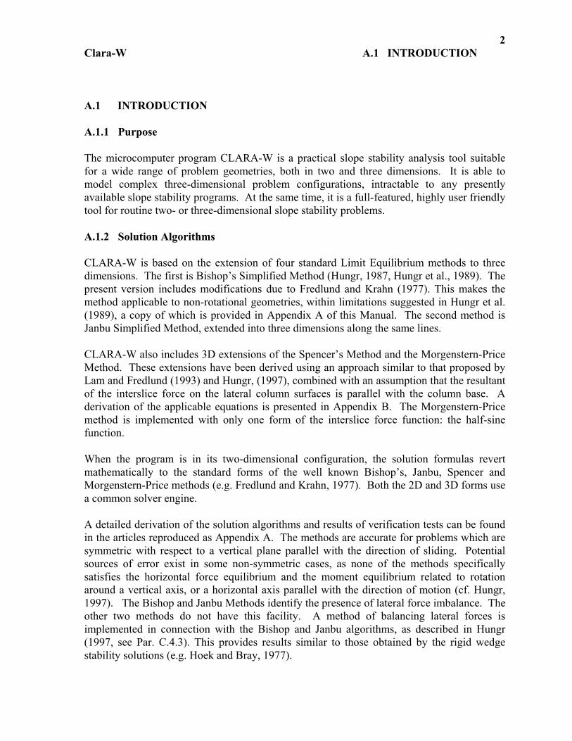
A.1 INTRODUCTION A.1.1 Purpose The microcomputer program CLARA-W is a practical slope stability analysis tool suitable for a wide range of problem geometries, both in two and three dimensions. It is able to model complex three-dimensional problem configurations, intractable to any presently available slope stability programs. At the same time, it is a full-featured, highly user friendly tool for routine two- or three-dimensional slope stability problems. A.1.2 Solution Algorithms CLARA-W is based on the extension of four standard Limit Equilibrium methods to three dimensions. The first is Bishop’s Simplified Method (Hungr, 1987, Hungr et al., 1989). The present version includes modifications due to Fredlund and Krahn (1977). This makes the method applicable to non-rotational geometries, within limitations suggested in Hungr et al. (1989), a copy of which is provided in Appendix A of this Manual. The second method is Janbu Simplified Method, extended into three dimensions along the same lines. CLARA-W also includes 3D extensions of the Spencer’s Method and the Morgenstern-Price Method. These extensions have been derived using an approach similar to that proposed by Lam and Fredlund (1993) and Hungr, (1997), combined with an assumption that the resultant of the interslice force on the lateral column surfaces is parallel with the column base. A derivation of the applicable equations is presented in Appendix B. The Morgenstern-Price method is implemented with only one form of the interslice force function: the half-sine function. When the program is in its two-dimensional configuration, the solution formulas revert mathematically to the standard forms of the well known Bishop’s, Janbu, Spencer and Morgenstern-Price methods (e.g. Fredlund and Krahn, 1977). Both the 2D and 3D forms use a common solver engine. A detailed derivation of the solution algorithms and results of verification tests can be found in the articles reproduced as Appendix A. The methods are accurate for problems which are symmetric with respect to a vertical plane parallel with the direction of sliding. Potential sources of error exist in some non-symmetric cases, as none of the methods specifically satisfies the horizontal force equilibrium and the moment equilibrium related to rotation around a vertical axis, or a horizontal axis parallel with the direction of motion (cf. Hungr, 1997). The Bishop and Janbu Methods identify the presence of lateral force imbalance. The other two methods do not have this facility. A method of balancing lateral forces is implemented in connection with the Bishop and Janbu algorithms, as described in Hungr (1997, see Par. C.4.3). This provides results similar to those obtained by the rigid wedge stability solutions (e.g. Hoek and Bray, 1977).

Clara-W A.1 INTRODUCTION
3
The Bishop, Spencer and Morgenstern-Price methods usually give similar results for rotational sliding surface geometries. There will be differences between the three methods in case of some non-rotational sliding surfaces, similar as experienced in two-dimensional analyses. The Janbu Method usually yields lower Factors of Safety than the other methods, both for rotational and non-rotational surfaces. Bishop’s Simplified Method may be inaccurate when used with horizontal external loads or large water thrusts. Spencer and Morgenstern-Price methods may fail to converge in some cases, or may yield unacceptable solutions. A.1.3 Typical Applications In its 2D configuration, CLARA-W can be applied to a range of routine problems, familiar to users of other slope stability programs. The 3D configuration is suitable for the following types of problems:
- Slopes curved or discontinuous in plan: ends and corners of embankments, narrow excavations, earth dam abutments and spillways, bridge approach fills, conical heaps, shafts, pits, ridges and re-entrants.
- Narrow failure surfaces: spoon-shaped slides, failures situated between lateral
constraints. - Slopes with significant lateral variation in steepness, failure surface geometry,
stratigraphy, strength properties, piezometric conditions, loads, or all of the above. - Complex wedge geometries with or without anchor support. - Slope failures under concentrated loading situated on the slope face or at the crest.
A.1.4 Copyright and Licensing CLARA-W is not copy-protected, in order to permit legitimate backup. It is copyrighted, however, and all rights of distribution are reserved by O. Hungr Geotechnical Research Inc. (OHGRI). Its use is permitted only to authorized licensees, under the terms and conditions of the licensing agreement signed between them and OHGRI. The name of the licensee appears on the program title screen. A.1.5 Precautions IMORTANT: General precautions common to any advanced geotechnical analysis should be followed (see Krahn, 2001). Specific precautions are listed below:
Clara-W A.1 INTRODUCTION
4
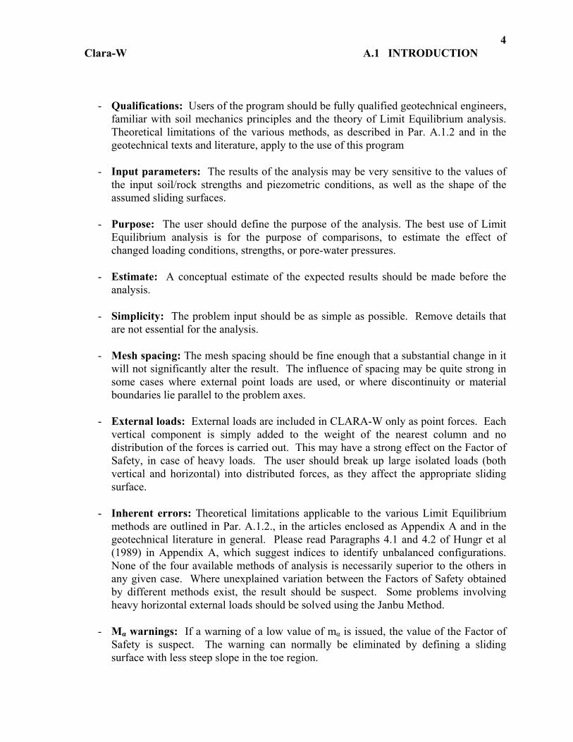
- Qualifications: Users of the program should be fully qualified geotechnical engineers, familiar with soil mechanics principles and the theory of Limit Equilibrium analysis. Theoretical limitations of the various methods, as described in Par. A.1.2 and in the geotechnical texts and literature, apply to the use of this program
- Input parameters: The results of the analysis may be very sensitive to the values of
the input soil/rock strengths and piezometric conditions, as well as the shape of the assumed sliding surfaces.
- Purpose: The user should define the purpose of the analysis. The best use of Limit
Equilibrium analysis is for the purpose of comparisons, to estimate the effect of changed loading conditions, strengths, or pore-water pressures.
- Estimate: A conceptual estimate of the expected results should be made before the
analysis. - Simplicity: The problem input should be as simple as possible. Remove details that
are not essential for the analysis.
- Mesh spacing: The mesh spacing should be fine enough that a substantial change in it will not significantly alter the result. The influence of spacing may be quite strong in some cases where external point loads are used, or where discontinuity or material boundaries lie parallel to the problem axes.
- External loads: External loads are included in CLARA-W only as point forces. Each
vertical component is simply added to the weight of the nearest column and no distribution of the forces is carried out. This may have a strong effect on the Factor of Safety, in case of heavy loads. The user should break up large isolated loads (both vertical and horizontal) into distributed forces, as they affect the appropriate sliding surface.
- Inherent errors: Theoretical limitations applicable to the various Limit Equilibrium
methods are outlined in Par. A.1.2., in the articles enclosed as Appendix A and in the geotechnical literature in general. Please read Paragraphs 4.1 and 4.2 of Hungr et al (1989) in Appendix A, which suggest indices to identify unbalanced configurations. None of the four available methods of analysis is necessarily superior to the others in any given case. Where unexplained variation between the Factors of Safety obtained by different methods exist, the result should be suspect. Some problems involving heavy horizontal external loads should be solved using the Janbu Method.
- Mα warnings: If a warning of a low value of mα is issued, the value of the Factor of
Safety is suspect. The warning can normally be eliminated by defining a sliding surface with less steep slope in the toe region.

Clara-W A.1 INTRODUCTION
5
- Negative normal stress: If the normal stress on the column base has a negative value in more than a few % of the slide volume, the Factor of Safety may be suspect. It may be necessary to include a tension crack to eliminate this condition.
- Other indices: In case of Spencer's or Morgenstern Price analyses, the thrust line
should be acceptable in more than about 75% of the slide volume and the internal strength should not be exceeded in more than a few % of the slide volume. Otherwise, the relevant Factors of Safety are suspect.
- Verification: Results should be verified by carrying out spot checks of selected
parameters against hand calculations and by comparing results with simplified solutions or against other analytical methods.
- Sliding Direction: CLARA-W resolves equilibrium only in the assumed direction of
sliding, i.e. the negative y-direction. The user must ensure that the mesh of columns is constructed in such a way that a kinematically viable sliding mechanism exists in that direction and that it is the most unfavourable direction of movement from the point of stability. For example, when analysing classical wedges formed of two intersecting planes, the mesh should be constructed so that the y-axis is exactly parallel with the intersection line.
A.1.6 How to Use This Manual It is recommended that engineers intending to use the program professionally should read the entire text of the Manual, including the Appendices. The manual is organized into four parts, distinguished by the header. Part A is a description of the program, explaining its various functions. Part B contains detailed instructions for using the program to input and manage data. Part C contains instructions for using the solution modules and receiving output. Part D is a brief set of instructions required to test run the program using Tutorial Examples supplied. Running these examples is perhaps the best way to become acquainted with the main functions of the program. To find out only what the capabilities of the program are, the user should read Paragraphs A.1.3 and A.1.7. Those interested in the theoretical background and in assessing the results accuracy under various conditions, should read Appendices A and B. An alphabetic listing of error and warning messages appears in Appendix D. A.1.7 List of Program Features
- General two or three-dimensional slope geometry with multiple material layers.
Clara-W A.1 INTRODUCTION
6
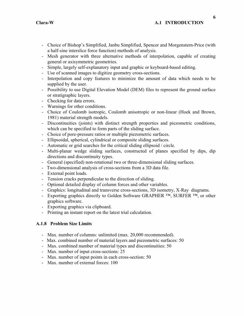
- Choice of Bishop’s Simplified, Janbu Simplified, Spencer and Morgenstern-Price (with a half-sine interslice force function) methods of analysis.
- Mesh generator with three alternative methods of interpolation, capable of creating general or axisymmetric geometries.
- Simple, largely self-explanatory input and graphic or keyboard-based editing. - Use of scanned images to digitize geometry cross-sections. - Interpolation and copy features to minimize the amount of data which needs to be
supplied by the user. - Possibility to use Digital Elevation Model (DEM) files to represent the ground surface
or stratigraphic layers. - Checking for data errors. - Warnings for other conditions. - Choice of Coulomb isotropic, Coulomb anisotropic or non-linear (Hoek and Brown,
1981) material strength models. - Discontinuities (joints) with distinct strength properties and piezometric conditions,
which can be specified to form parts of the sliding surface. - Choice of pore-pressure ratios or multiple piezometric surfaces. - Ellipsoidal, spherical, cylindrical or composite sliding surfaces. - Automatic or grid searches for the critical sliding ellipsoid / circle. - Multi-planar wedge sliding surfaces, constructed of planes specified by dips, dip
directions and discontinuity types. - General (specified) non-rotational two or three-dimensional sliding surfaces. - Two-dimensional analysis of cross-sections from a 3D data file. - External point loads. - Tension cracks perpendicular to the direction of sliding. - Optional detailed display of column forces and other variables. - Graphics: longitudinal and transverse cross-sections, 3D isometry, X-Ray diagrams. - Exporting graphics directly to Golden Software GRAPHER ™, SURFER ™, or other
graphics software. - Exporting graphics via clipboard. - Printing an instant report on the latest trial calculation.
A.1.8 Problem Size Limits
- Max. number of columns: unlimited (max. 20,000 recommended). - Max. combined number of material layers and piezometric surfaces: 50 - Max. combined number of material types and discontinuities: 50 - Max. number of input cross-sections: 25 - Max. number of input points in each cross-section: 50 - Max. number of external forces: 100

Clara-W A.2 INPUT DATA ORGANIZATION
7
A.2 INPUT DATA ORGANIZATION A.2.1 Data Files Each file contains all the input data describing a slope problem, including material and discontinuity properties and the geometry of material and piezometric surfaces. The file name is specified by the user. CLARA-W appends the file name with an extension .CLW. The data file should be saved frequently during each editing session. A.2.2 Coordinate System CLARA-W uses a Cartesian coordinate system as shown in Fig. A.1. The origin is located at or beyond the left-hand margin of the problem mesh, looking in the direction of movement. Axis X is horizontal and perpendicular to the movement direction. Axis Y is opposite to the movement direction. Axis Z is vertical. MESH ALIGNMENT: 1) The analysis must always be carried out so that the slope falls from right to left, in
the negative-Y direction. The “Edit-Geometry Options- Mirror” feature allows the user to rotate any existing geometry to the correct sense.
2) The user is responsible for aligning the Y-axis parallel with the direction of motion. The equilibrium equations are resolved in the Y-direction. Should the actual movement direction be different, the factor of safety may be overestimated. CLARA-W permits small perturbation of the direction in which the equilibrium equations are resolved, as described in Par. C.1.5, to examine the effect of movement direction. However, it is preferable to have the mesh oriented correctly, as the rotation feature may not always produce results of comparable accuracy. If in doubt, set up several column assemblies with different orientations of the coordinate system and seek the direction which yields the least factor of safety.
A.2.3 Column Assembly (“Mesh”) The analysis is carried out on an assembly of columns of equal rectangular plan referred to as the mesh, as shown in Fig. A.1. To define the problem extent, the user specifies the following:
- mesh limits in the X- (transverse) direction: XS (start, left margin) and XE (end, right margin).
- mesh limits in the Y-direction (direction of motion): YS (start, near the toe) and YE (end, near the crest of the slope).
- number of rows, NX and the number of columns in each row, NY.
Clara-W A.2 INPUT DATA ORGANIZATION
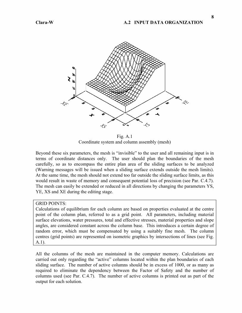
8
Fig. A.1 Coordinate system and column assembly (mesh)
Beyond these six parameters, the mesh is “invisible” to the user and all remaining input is in terms of coordinate distances only. The user should plan the boundaries of the mesh carefully, so as to encompass the entire plan area of the sliding surfaces to be analyzed (Warning messages will be issued when a sliding surface extends outside the mesh limits). At the same time, the mesh should not extend too far outside the sliding surface limits, as this would result in waste of memory and consequent potential loss of precision (see Par. C.4.7). The mesh can easily be extended or reduced in all directions by changing the parameters YS, YE, XS and XE during the editing stage. GRID POINTS: Calculations of equilibrium for each column are based on properties evaluated at the centre point of the column plan, referred to as a grid point. All parameters, including material surface elevations, water pressures, total and effective stresses, material properties and slope angles, are considered constant across the column base. This introduces a certain degree of random error, which must be compensated by using a suitably fine mesh. The column centres (grid points) are represented on isometric graphics by intersections of lines (see Fig. A.1). All the columns of the mesh are maintained in the computer memory. Calculations are carried out only regarding the “active” columns located within the plan boundaries of each sliding surface. The number of active columns should be in excess of 1000, or as many as required to eliminate the dependency between the Factor of Safety and the number of columns used (see Par. C.4.7). The number of active columns is printed out as part of the output for each solution.
Clara-W A.2 INPUT DATA ORGANIZATION
9
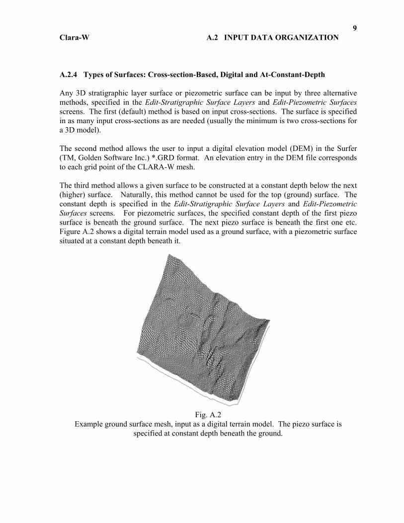
A.2.4 Types of Surfaces: Cross-section-Based, Digital and At-Constant-Depth Any 3D stratigraphic layer surface or piezometric surface can be input by three alternative methods, specified in the Edit-Stratigraphic Surface Layers and Edit-Piezometric Surfaces screens. The first (default) method is based on input cross-sections. The surface is specified in as many input cross-sections as are needed (usually the minimum is two cross-sections for a 3D model). The second method allows the user to input a digital elevation model (DEM) in the Surfer (TM, Golden Software Inc.) *.GRD format. An elevation entry in the DEM file corresponds to each grid point of the CLARA-W mesh. The third method allows a given surface to be constructed at a constant depth below the next (higher) surface. Naturally, this method cannot be used for the top (ground) surface. The constant depth is specified in the Edit-Stratigraphic Surface Layers and Edit-Piezometric Surfaces screens. For piezometric surfaces, the specified constant depth of the first piezo surface is beneath the ground surface. The next piezo surface is beneath the first one etc. Figure A.2 shows a digital terrain model used as a ground surface, with a piezometric surface situated at a constant depth beneath it.
Fig. A.2 Example ground surface mesh, input as a digital terrain model. The piezo surface is
specified at constant depth beneath the ground.
Clara-W A.2 INPUT DATA ORGANIZATION
10
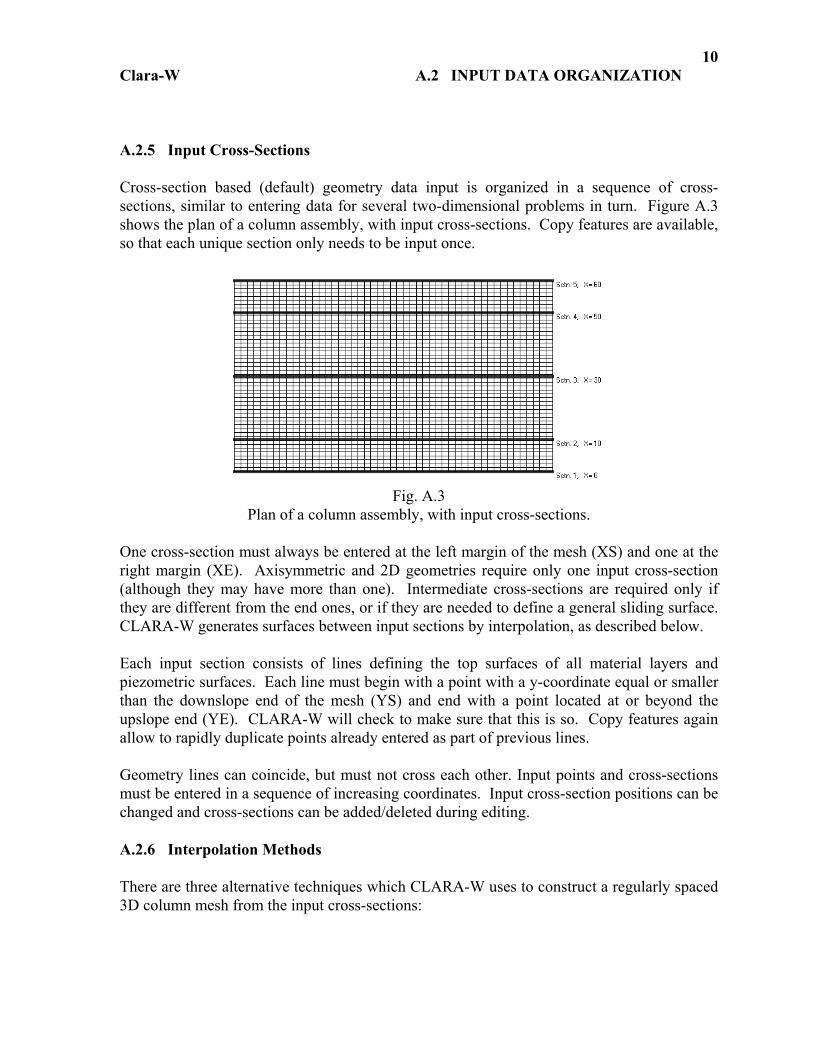
A.2.5 Input Cross-Sections Cross-section based (default) geometry data input is organized in a sequence of cross-sections, similar to entering data for several two-dimensional problems in turn. Figure A.3 shows the plan of a column assembly, with input cross-sections. Copy features are available, so that each unique section only needs to be input once.
Fig. A.3
Plan of a column assembly, with input cross-sections.
One cross-section must always be entered at the left margin of the mesh (XS) and one at the right margin (XE). Axisymmetric and 2D geometries require only one input cross-section (although they may have more than one). Intermediate cross-sections are required only if they are different from the end ones, or if they are needed to define a general sliding surface. CLARA-W generates surfaces between input sections by interpolation, as described below. Each input section consists of lines defining the top surfaces of all material layers and piezometric surfaces. Each line must begin with a point with a y-coordinate equal or smaller than the downslope end of the mesh (YS) and end with a point located at or beyond the upslope end (YE). CLARA-W will check to make sure that this is so. Copy features again allow to rapidly duplicate points already entered as part of previous lines. Geometry lines can coincide, but must not cross each other. Input points and cross-sections must be entered in a sequence of increasing coordinates. Input cross-section positions can be changed and cross-sections can be added/deleted during editing. A.2.6 Interpolation Methods There are three alternative techniques which CLARA-W uses to construct a regularly spaced 3D column mesh from the input cross-sections:

Clara-W A.2 INPUT DATA ORGANIZATION
11
1) Orthogonal Interpolation: As illustrated in Fig. A.4a, this involves linear interpolation between each pair of adjacent input points, first in the Y-direction and then in the X-direction from one cross-section to another. This method is most suitable for uniform geometries, or for general geometries or specified sliding surfaces. An example is shown in Fig. A.4b.
2) Oblique Interpolation: With this option, interpolation occurs first in the oblique
directions between each pair of input points located in adjacent cross-sections. The rest of the mesh is filled by interpolating in the Y-direction (Fig. A.5a). Each input cross-section must have the same number of points, otherwise an incomplete mesh would result. The method is especially suitable for surfaces containing inclined planar segments, such as man-made embankments or cuttings (Fig. A.5b). General (specified) sliding surfaces cannot be used with this option.
3) Axisymmetric Interpolation: Only one cross-section needs to be input with this
option. The column mesh will be generated by rotating this cross-section around a vertical axis, placed at any selected pair of X and Y-coordinates. The rotation radius is always measured in the y-direction, as if the input cross-section was located at the same X-coordinate as the rotation centre (see Fig. A.6a). All the surfaces defined in the cross-section are rotated, including piezometric surfaces. A concave slope will result from a centre located downslope from the toe; a convex one if the centre is located beyond the slope crest (Fig. A.6b). General sliding surfaces cannot be used.
Fig. A.4
a) Orthogonal interpolation. b) Example of a slope surface created by orthogonal interpolation

Clara-W A.2 INPUT DATA ORGANIZATION
12
Fig. A.5
a) Oblique interpolation. b) Surface generated from the same data, using oblique interpolation.
Fig. A.6
a) Axisymmetric interpolation method. b) Example result.

Clara-W A.2 INPUT DATA ORGANIZATION
13
A.2.7 Sliding Surfaces Sliding surfaces are generated by the solution modules, independently of the problem data file. A given slope problem can thus be analyzed with respect to five types of surfaces:
- An ellipsoidal surface is symmetrical around a horizontal axis of rotation, perpendicular to the direction of sliding. Each ellipsoid is specified by the coordinates of its centre, the elevation of a horizontal tangent plane and an aspect ratio (Fig. A.7). The aspect ratio is the ratio between ellipsoid semi-axes perpendicular and parallel with the direction of sliding. A ratio of 1.0 defines a spherical surface. A very large number (e.g. 1,000) locally defines a cylinder.
- Multi-planar wedges are non-rotational surfaces assembled from up to 10 planes
with various orientations and surface properties such as joints, seams or faults (Fig. A.8). The planes are specified by dip and dip-direction angles and positions in space. The program does not calculate the intersections of the planes, but assembles the wedge by choosing the highest situated plane below ground surface at each column center. The user must ensure beforehand that movement of the wedge is kinematically feasible and that the movement direction is correct. Discontinuity properties can be assigned to each individual plane, to over-ride the properties of the material. This is suitable for modeling structurally-controlled rupture surfaces which follow discontinuities in the soil or rock.
IMPORTANT: CLARA-W is less suited to classical two-plane wedge solutions than rigid-body wedge programs and should not be extensively used for these surfaces.
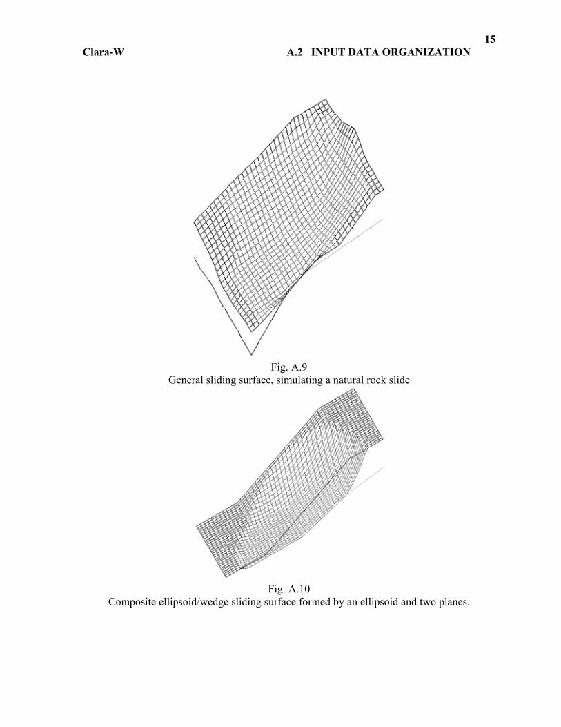
- A general (specified) surface is a surface of arbitrary shape, assembled in the same way as any other surface, e.g. a material surface. This module is useful for modeling irregular surfaces of known geometry, especially those in existing slides (Fig. A.9).
- A composite ellipsoid/wedge surface is a combination of an ellipsoid and a wedge.
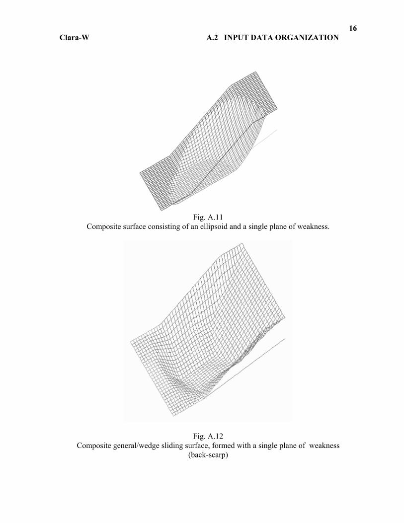
An ellipsoidal surface is truncated by a wedge composed of one or several planes specified by their reference points, dips and dip directions (Fig. A.10). In any given column, the highest of the two surfaces will be effective, resulting in an ellipsoid, truncated by planes. The simplest type of a composite surface is an ellipsoid truncated by a single plane, such as a planar surface of weakness (Fig. A.11). Discontinuity properties and piezo conditions may or may not be associated with the individual wedge-forming planes, as described in Par. C.2.7.
- A composite general/wedge surface is similarly made-up of a cross-section
specified surface, truncated by a wedge made up of one or several planes (Fig. A.12). In any given column, the higher of the two surfaces will be effective, resulting in a general surface, truncated by planes. The simplest type of composite surface is a

Clara-W A.2 INPUT DATA ORGANIZATION
14
general surface truncated by a single plane, such as a planar surface of weakness. Discontinuities may or may not be associated with the individual wedge-forming planes, as described in Par. C.2.7.
- The parameters of each type of the latest surface used are saved in the problem data file. This enables the user to interrupt and re-commence work with a variety of sliding surfaces or searches as required.
Fig. A.7
Example ellipsoidal sliding surface.
Fig. A.8
Example of a multi-planar wedge.
Clara-W A.2 INPUT DATA ORGANIZATION
15
Fig. A.9
General sliding surface, simulating a natural rock slide
Fig. A.10
Composite ellipsoid/wedge sliding surface formed by an ellipsoid and two planes.
Clara-W A.2 INPUT DATA ORGANIZATION
16
Fig. A.11
Composite surface consisting of an ellipsoid and a single plane of weakness.
Fig. A.12 Composite general/wedge sliding surface, formed with a single plane of weakness
(back-scarp)
Clara-W A.2 INPUT DATA ORGANIZATION
17
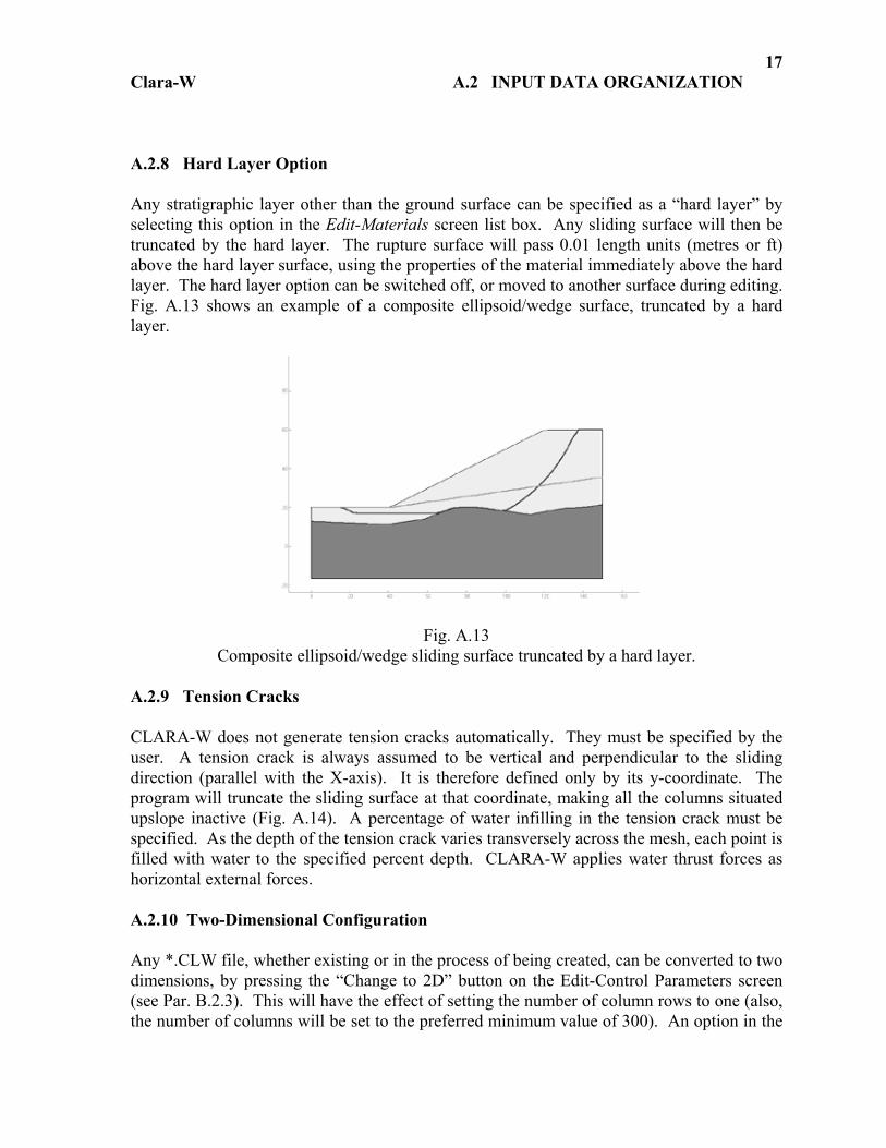
A.2.8 Hard Layer Option Any stratigraphic layer other than the ground surface can be specified as a “hard layer” by selecting this option in the Edit-Materials screen list box. Any sliding surface will then be truncated by the hard layer. The rupture surface will pass 0.01 length units (metres or ft) above the hard layer surface, using the properties of the material immediately above the hard layer. The hard layer option can be switched off, or moved to another surface during editing. Fig. A.13 shows an example of a composite ellipsoid/wedge surface, truncated by a hard layer.
Fig. A.13 Composite ellipsoid/wedge sliding surface truncated by a hard layer.
A.2.9 Tension Cracks CLARA-W does not generate tension cracks automatically. They must be specified by the user. A tension crack is always assumed to be vertical and perpendicular to the sliding direction (parallel with the X-axis). It is therefore defined only by its y-coordinate. The program will truncate the sliding surface at that coordinate, making all the columns situated upslope inactive (Fig. A.14). A percentage of water infilling in the tension crack must be specified. As the depth of the tension crack varies transversely across the mesh, each point is filled with water to the specified percent depth. CLARA-W applies water thrust forces as horizontal external forces. A.2.10 Two-Dimensional Configuration Any *.CLW file, whether existing or in the process of being created, can be converted to two dimensions, by pressing the “Change to 2D” button on the Edit-Control Parameters screen (see Par. B.2.3). This will have the effect of setting the number of column rows to one (also, the number of columns will be set to the preferred minimum value of 300). An option in the

Clara-W A.2 INPUT DATA ORGANIZATION
18
“Graphics-Export” menu allows the user to record a 2D *.CLW file at a given x-coordinate in the current directory while working with a 3D model (including problems containing surfaces defined by *.GRD files).
Fig. A.14
Ellipsoidal sliding surface with a tension crack.
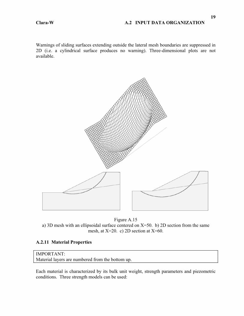
If a file is specified as two-dimensional at the point of being created, it is sufficient to have only one input cross-section, situated at an X coordinate of zero. CLARA-W will then operate like any 2D program and no interpolation will be done. If a file is converted from 3D to 2D by pressing the “Change to 2D” button, the interpolation procedures will still be carried out. However, these will be done only with respect to a 2D “mesh” consisting of one row of columns, situated at an X-coordinate specified by the minimum X (XS) variable. In this way, any selected 2D section from a 3D file can be analyzed. Another section can be set up simply by changing XS in the Control Parameters screen. The file can be converted back to 3D by pressing the “Change to 3D” button and re-entering the appropriate values for minimum X (XS) and maximum X (XE). Figure A.15a shows an example of a 3D mesh with an ellipsoidal surface centered at X=50m. Two sections, at X=20 and X=60 are shown in Figures A.15b and c.
Whenever the program is in the 2D configuration, all lateral slope angles are zero. Apart from this, the solution of a 2D mesh is carried out by the same routines that are used for a 3D analysis. The solver routines of CLARA-W recognize no difference between a mesh consisting of many rows, or one containing only a single row of columns.
Clara-W A.2 INPUT DATA ORGANIZATION
19
Warnings of sliding surfaces extending outside the lateral mesh boundaries are suppressed in 2D (i.e. a cylindrical surface produces no warning). Three-dimensional plots are not available.
Figure A.15 a) 3D mesh with an ellipsoidal surface centered on X=50. b) 2D section from the same
mesh, at X=20. c) 2D section at X=60. A.2.11 Material Properties IMPORTANT: Material layers are numbered from the bottom up. Each material is characterized by its bulk unit weight, strength parameters and piezometric conditions. Three strength models can be used:

Clara-W A.2 INPUT DATA ORGANIZATION
20
a) Coulomb isotropic strength is the routine strength model, characterized by a friction angle and a cohesion.
b) Anisotropic Coulomb strength requires two values each of cohesion and friction
angle, specified for the horizontal and vertical orientations of the sliding surface. The actual values used in each column depend on the dip angle of the sliding surface in that column, following an elliptic function defined in Appendix C. They can be viewed using the detailed output option. Typical use of this model is for a thinly horizontally interbedded sequence of weak and strong layers.
c) Non-linear model uses a parabolic shear strength envelope as developed by Hoek and
Brown (1980, Chapter 6 - see reference in Appendix C), characterized by four constants. CLARA-W uses the model to calculate an apparent cohesion and a friction angle in each iteration, based on the effective normal stress at the base of each column (see Appendix C). The solution algorithm is not influenced by the use of the non-linear model. Table 12 of Hoek and Brown (1980) gives typical values of the parameters for jointed rock masses. Values for other materials (e.g. rockfill) can be derived from laboratory or field test data by curve fitting.
A.2.12 Discontinuities Discontinuity properties are defined in the same way as those of materials. While material properties are assigned to the rupture surface depending on its position within the stratigraphy, discontinuity properties are imposed on specific parts of the sliding surface by one of the following means:
a) Properties of a discontinuity can be associated with the plane part of a composite ellipsoid-plane surface (cf. Fig. A.11).
b) A different discontinuity type can be assigned to each of several planes forming a
multi-planar wedge, or to a specified “field” of a general surface.
Various discontinuity types are referenced by code numbers. Whenever a reference is made to Discontinuity Code 0, this means that material properties corresponding to the stratigraphy will be used over that part of the sliding surface. Discontinuities may be defined and not used. Their use is specified only at the time of referencing a discontinuity code number in connection with one of the above geometries. A.2.13 Piezometric Conditions Pore-pressures acting on the sliding surface can be specified by three methods, as described in Fig. A.16 and below:

Clara-W A.2 INPUT DATA ORGANIZATION
21
a) A pore-pressure ratio “ru” can be associated with a material or a discontinuity. The pore-pressure will be calculated by multiplying the total vertical stress at the centre of each column base by the ratio:
uru σ= Eqn.[1]
Here, σ is the total vertical overburden stress at a point and u is the pore pressure. When ru is zero, there is no pore-pressure, unless there is a piezo surface.
b) A piezometric surface of a given number can be associated with a material or a
discontinuity. The pore-pressure will be calculated as the hydrostatic pressure corresponding to the elevation of the piezo surface above the base of each column.
IMPORTANT: The use of a particular piezometric surface is specified by referencing its number in course of the definition of material/ discontinuity properties. Piezo surfaces may thus be defined and shown in plots, but not used in the analysis. CLARA-W will issue a warning during analysis where this is the case. Always check for proper pore-pressure ratio/piezo surface specification for each material, as listed in the properties summary table supplied in the output. Also, carry out spot checks of pore pressure in detailed output.
c) A “ B ” value can be entered for each material layer other than the uppermost material. If a non-zero B value is specified for a material, the piezometric pressures in that material will be increased by adding an excess pore-pressure equal to B times the total weight of the uppermost layer (“fill”):
ffww hBhu γγ +=∆ Eqn. [2]
where γw is the unit weight of water, γf is the unit weight of the fill and hw and hf are defined in Fig. A.16.
Fig. A.16 Three alternative methods of piezometric pressure specifications.
hw
hf
hw
h

Clara-W A.2 INPUT DATA ORGANIZATION
22
IMPORTANT: The user must keep in mind the difference between a piezometric surface and the phreatic surface (water table) as explained in texts of hydrogeology. A.2.14 Toe Submergence Water is specified using a list box in the Edit-Materials screen. It will be characterized by zero strength and the appropriate unit weight. No other provisions need be made to analyze a submerged slope. As an alternative to the above method, submerged weights for material located below the water table can be used. No water stratum should then be specified. A material specified as "water" should always be the uppermost material over that part of the mesh where it is of non-zero thickness. When a fluid is encountered, the program will truncate the sliding surface as shown in Fig. A.17 and automatically apply a horizontal hydrostatic thrust pressure corresponding to the water depth. The magnitude of the thrust pressure is printed during output.
Fig. A.17
Automatic adjustments for submergence made by the program. Water can be located only at the toe of the sliding surface. CLARA-W cannot analyze situations where the head of the slide is submerged (such as at the crest of a full reservoir). An error message will be issued in these cases. A.2.15 External Loads Up to 100 point loads can be specified. Each load is defined by the x, y and z coordinates of its point of application, and its horizontal (Py) and vertical (Pz) components. The loads have no lateral (x) components. IMPORTANT: External loads are included in CLARA-W only as point forces. Each vertical component is simply added to the weight of the nearest column and no distribution of the forces is carried out. This may have a strong effect on the Factor of Safety, in case of heavy loads. The user should break up large isolated loads (both vertical and horizontal) into distributed forces, as they affect the appropriate sliding surface.

Clara-W A.2 INPUT DATA ORGANIZATION
23
The vertical component of each external force located within the sliding area boundaries is added to the total weight of the column directly beneath, irrespective of the elevation at which the force is applied (it may even be above ground). The horizontal components of the external forces are included in the moment or horizontal force equilibrium equations (see Eqns. 1 and 3, of Hungr et al., 1989, see Appendix A). IMPORTANT: The vertical components of any forces situated outside the plan outline of the sliding surface or beneath the sliding surface will not be included in the calculation. The horizontal components of any forces where the horizontal projection of the force does not intersect the sliding body will also not be included in the calculations. In 2D analyses, the external forces must lie in the plane of the section being analyzed. External loads are line loads in the 2D configuration, with units of force per unit width. External force components not used in calculations will not appear in graphics displayed after analysis and will not be added to the external force totals presented in the output. The latter feature can be used to check whether any forces have been left out of the analysis.
Clara-W A.3 PROGRAM CONTROL
24
A.3 PROGRAM CONTROL A.3.1 The Main Menu The program flow is controlled primarily by the Main Menu (see Fig. B.3), which allows the user to select both the main utility functions and solution types. The Main Menu returns at the conclusion of each function or solution. Some menu items are disabled or enabled at times, depending on their availability. The following is a list of all the options found in the Main Menu with a short description of each: - File: The options under this menu deal with file manipulation. This menu is enabled at all
times.
- File-New: Opens a new file with all data either empty or set to a default value. Also initializes the Input Sequence (see Par. B.2.2), which guides the user through the process of creating a new problem file. Shortcut key → Ctrl+N.
- File-Open: Allows the user to open a previously saved *.CLW file. Shortcut key
→ Ctrl+O.
- File-Save: Saves the current project in the current directory and under the current *.CLW file name. Shortcut key → Ctrl+S.
- File-Save As: Allows the user to save the current project in any available directory
as a *.CLW file.
- File-Open *.CLA File: Allows the user to open a *.CLA file previously created and saved in CLARA (DOS version).
- File-Print:
- Current View: Sends the current screen graphic to the default system printer. Shortcut key → Ctrl+P.
- File-Exit: Ends and closes CLARA-W. The user is prompted to save the current
file before the program closes.
- Edit: Options under this menu allow separate editing of the problem geometry, material and discontinuity properties, external forces, and tension crack screens. This menu is enabled only when a file is loaded.
- Edit-Control Parameters: Opens the Control Parameters Screen (see Par. B.2.3)
which allows the user to input and modify the current file's identifying labels,
Clara-W A.3 PROGRAM CONTROL
25
problem boundaries, mesh spacing, units and earthquake acceleration. This screen also allows the user to switch from 2D to 3D or vice versa.
- Edit-Material Properties: Opens the Material Properties screen (see Par. B.2.5)
which allows the user to input and edit the current problem's material properties as described in Par. A.2.11. This screen also allows the user to add and delete discontinuity layers.
- Edit-Stratigraphic Layer Surfaces: Opens the Stratigraphic Layer Surfaces screen
(see Par. B.2.7) which allows the user to define the type of input surface used for each layer as described in Par. A.2.4. This is the only screen which allows the user to add and delete stratigraphic layers.
- Edit-Piezometric Surfaces: Opens the Piezometric Surfaces screen (see Par. B.2.8)
which allows the user to define the type of input surface used for each piezo surface as described in Par. A.2.4. This screen also allows the user to add and delete piezo surfaces.
- Edit-Cross-section Positions: Opens the Cross-section Positions screen (see Par.
B.2.9) which allows the user to define the position along the X-axis of each cross-section for cross-section-based layers and surfaces. This screen also allows the user to add and delete cross-sections or move existing cross-sections to different positions.
- Edit-Cross-sections: Opens the Edit Cross-sections screen (see Par. B.3.1) which
allows the user to input or edit geometry data for any cross-section.
- Edit-External Forces: Opens the External Forces screen (see Par. C.1.3) which allows the user to define the application coordinates and the vertical and horizontal components of any external forces acting on the surface. This screen also allows the user to add and delete forces.
- Edit-Tension Crack: Opens the Tension Crack screen (see Par. C.1.4) which
allows the user to input a tension crack as described in Par. A.2.9.
- Edit-Geometry Options: - Edit-Geometry Options-Interpolation: Opens the Interpolation Method
screen (see Par. B.2.4) which allows the user to select one of the three interpolation methods as described in Par. A.2.6.
- Edit-Geometry Options-Mirror: Allows the user to rotate any existing
geometry by 180 degrees. As specified in Par. A.2.2, the slope being
Clara-W A.3 PROGRAM CONTROL
26
analyzed by CLARA-W should always face from right to left. This option is useful to invert existing geometries which slope in the wrong direction.
- Surface: The options under this menu allow the user to define either a single sliding
surface or a search. This menu is enabled only when a file is loaded.
- Surface-Ellipsoid:
- Single Ellipsoidal Surface: Opens the Single Ellipsoidal Surface Input screen (see Par. C.2.1) which allows the user to enter an ellipsoidal, spherical, or cylindrical sliding surface as described in Par. A.2.7.
- Grid Search: Opens the Grid Search Input screen (see Par. C.2.3) which
allows the user to set up an ellipsoidal grid search as described in Par. C.2.2.
- Auto Search: Opens the Auto Search Input screen (see Par. C.2.5) which
allows the user to set up an ellipsoidal auto search as described in Par. C.2.4.
- Surface-Wedge: Opens the Multi-Planar Wedge Surface Input screen (Par. C.2.7)
which allows the user to set up the planes that make up a wedge sliding surface as described in Par. A.2.7.
- Surface-General: Begins the General Sliding Surface Sequence (Par. C.2.8) which
allows the user to enter a general, cross-section specified sliding surface into the problem, as described in Par. A.2.7.
- Surface-Composite-Ellipsoid/Wedge:
- Single Composite Surface: Begins the Composite Ellipsoid/Wedge Surface
Sequence (see Par. C.2.9) which allows the user to enter a single composite ellipsoid/wedge sliding surface into the problem as described in Par. A.2.7.
- Grid Search: Begins the Composite Ellipsoid/Wedge Grid Search
Sequence (see Par. C.2.9) which allows the user to set up a composite ellipsoid/wedge grid search as described in Par. C.2.2 and C.2.3.
- Auto Search: Begins the Composite Ellipsoid/Wedge Auto Search
Sequence (see Par. C.2.9) which allows the user to set up a composite ellipsoid/wedge auto search as described in Par. C.2.4 and C.2.5.
Clara-W A.3 PROGRAM CONTROL
27
- Surface-Composite-General/Wedge: Begins the Composite General/Wedge Surface Sequence (see Par. C.2.10) which allows the user to enter a single composite general/wedge sliding surface into the problem as described in Par. A.2.7.
- Solve: The options under this menu activate the solver routines for the corresponding
input sliding surface or search. The availability of these options depends on the type of sliding surface or search entered into the problem.
- Solve-Single Trial Surface: Activates the solver routine for a single trial surface of
any type, as described in Par. A.1.2. The Plan of Active Columns screen (see Par. C.4.1) is displayed. This option is only available if a single sliding surface of any type has been created.
- Solve-Grid Search: Activates the Grid Search Solve routine as described in Par.
C.2.6. This option is only available if a grid search of any type has been set up.
- Solve-Auto Search: Activates the Automatic Search Solve routine as described in Par. C.2.6. This option is only available if an auto search of any type has been set up.
- Solve-Set Rotation Angle: Opens the Rotation Angle screen which allows the user
to change the direction in which the equilibrium equations are resolved, as described in Par. C.1.5. Once a file has been opened, this option is available at all times. However, a non-zero rotation angle can be specified only for a single sliding surface (not for a search).
- Results: The Options under this menu deal with the printable “instant report” on the latest
trial calculation. This menu is always available.
- Results-Preview Report: Allows the user to view the report on screen before printing it, as described in Par. C.4.4.
- Results-Print Report: Sends the report directly to the printer, as described in Par.
C.4.4.
- Results-Save Report in *.txt File: Allows the user to save the text of the instant report in a *.txt file which can then be opened and modified in a word processor (see Par. C.4.4).
- Graphics: The options under this menu deal with the various screen graphics available in
CLARA-W.
Clara-W A.3 PROGRAM CONTROL
28
- Graphics-Isometry: Draws the appropriate three-dimensional isometric view of the chosen layer. The currently drawn layer is checked. This option is not available when the currently loaded file is in a two-dimensional form.
- Graphics-Longitudinal Section: Displays a longitudinal cross-sectional view of the
problem and allows the user to scroll this view through the mesh along the X-axis. This option is only available when a file is loaded.
- Graphics-Lateral Section: Displays a lateral cross-sectional view of the problem
and allows the user to scroll this view through the mesh along the Y-axis. This option is not available for two-dimensional problems.
- Graphics-Plan: Displays the plan view of the mesh, showing the positions of the
input cross-sections in red. This option is only available when a file is loaded.
- Graphics-X-ray: Displays an x-ray view of the geometry. This option is not available for two-dimensional problems.
- Graphics-Copy to Clipboard: Places the current screen graphic on the clipboard.
Shortcut key → Ctrl+C.
- Graphics-Export: - Isometry: *.GRD file: Allows the user to export the chosen three-
dimensional isometric view as a digital elevation model (DEM) in the Surfer (TM, Golden Software Inc.) *.GRD format.
- Two-dimensional .CLW file: Create a separate 2D file. - Longitudinal Section *.DAT File: Allows the user to export a selected
longitudinal cross-section view at a specified X-coordinate in *.DAT (ASCII) format, suitable for processing by Grapher (TM, Golden Software Inc.), or other compatible graphing software.
- Lateral Section *.DAT File: Allows the user to export a lateral cross-
section view at a specified Y-coordinate in *.DAT format. - Options: The items under this menu access various screens and graphical options and
preferences. This menu is enabled at all times.
- Options-Grid: Turns the background grid on or off in the Edit Cross-Sections screen, as described in Par. B.3.1.
Clara-W A.3 PROGRAM CONTROL
29
- Options-Graphics Options: Opens the Graphics Options screen (see Par. C.3.2) which allows the user to change the vertical exaggeration ratio, the cross-section fill style, and the isometry rotation angle.
- Colours: Opens the Colour Editor screen (see Par. C.3.3) which allows the user to
change the colours used for the graphics in the current file. - Window: Allows the user to access any of the currently open windows in the main screen
only. - Help: Provides access to the CLARA-W Help system, as well as copyright and licensing
information about CLARA-W. Secondary menus are used by all the Edit and Surface modules. The first and last menu options on all these secondary menus are Continue and Cancel, respectively. The Continue option places all the current information in that module into memory, applies it to the problem, and then returns to the main screen. The Cancel option exits the module without saving or applying any new information. CAUTION: The Cancel option should be used with care if in the middle of a sequence. It is better to finish a sequence and then redo it completely, rather than exit in the middle and potentially leave some unwanted information in the memory. A.3.2 Input Screens Apart from the main screen, CLARA-W input is carried out through secondary screens, each with their own menus. The secondary screens accept graphical or tabular input and user instructions. There are input screens, sliding surface screens, and solution screens. All the secondary screens are accessed from the main screen menu as described in the previous paragraph. The input screens are described in detail in Section B.2. The sliding surface and solution screens are described in Section C.2. A.3.3 Error/warning Messages CLARA-W keeps an eye out for a variety of input errors or other conditions which could potentially reduce the accuracy of the results. For an interpretation of the meaning of the individual messages, see Appendix D, where they are listed alphabetically. Many of the warning messages are of little consequence, in which case, the program will continue running. Others, however, may be important and CLARA-W will generally not accept the unsuitable input and will wait for it to be changed.

Clara-W A.3 PROGRAM CONTROL
30
The solver modules also have error and warning messages (listed in Appendix D). These are kept track of and counted for individual trial surfaces. Their number is reported as part of the output and the messages themselves are displayed in a separate window for each individual surface, after the solver module has finished running (see Par. C.4.2). During searches, messages are issued in connection with each individual trial surface rather than for all the surfaces as a whole. If you wish to see the specific messages, reanalyze the surface in question using the single ellipsoid or composite module.

31
_________________________________
PART B
DATA INPUT AND MANAGEMENT
_________________________________
Clara-W B.1 STARTING THE PROGRAM
32
B.1 STARTING THE PROGRAM B.1.1 General Run program Setup in the distribution folder. This will install CLARA-W and its Help Files in a chosen sub-directory on the hard drive. If setup does not work, it is sometimes possible to start the program by double-clicking the CLW.EXE file. The user may create a shortcut to CLARA-W using Windows facilities. Run CLARA-W through the Start menu, or by double-clicking its name or shortcut. On starting, CLARA-W presents a title screen which disappears by clicking the mouse or any key on the keyboard. An Initial Menu appears, prompting for one of three choices:
- Create a new file - Open an existing file - Other
The last choice opens the main screen and enables the Main Menu, with no file in the memory. B.1.2 Opening and Saving a Data File Using the menu selection File-Open, a *.CLW file can be read into the memory. The file will bring with it information concerning all the recent sliding surface and/or search parameters. In the case that any of the surfaces in the file are specified by DEM files, CLARA-W will attempt to open the appropriate *.GRD files in the directories where they were when the problem file was saved. Should the *.GRD files be erased or moved to other locations in the meantime, an error message will appear. The user may then browse for the applicable *.GRD files from the Stratigraphic Surfaces screen. CLARA-W can also read data files created by DOS CLARA, with an extension .CLA. Please note that not all data regarding searches will be correctly read from the *.CLA files and thus the search specifications may have to be re-defined by the user. To escape file opening, pressing the Cancel button will bring back the Main Menu. Names of files not in the current directory, misspelled names or names with wrong extensions will produce error messages. Selections File-Save and File-Save As will save the *.CLW file on the disk. IMPORTANT: CLARA-W will not function properly on computers where the decimal marker is a comma. The user must specify the use of a period in Windows International Settings.

Clara-W B.1 STARTING THE PROGRAM
33
Clara-W B.3 GEOMETRY INPUT
34
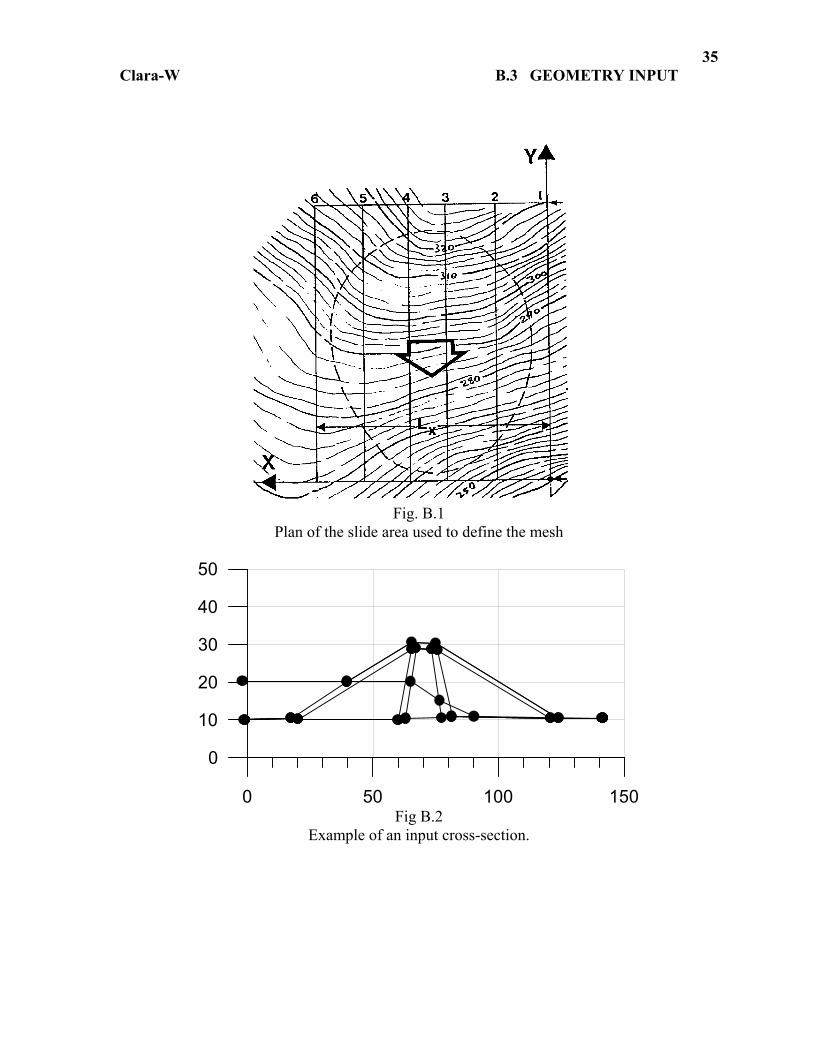
B.2 CREATING AN INPUT DATA FILE B.2.1 Data Preparation The preparation of a data file should begin with a plan of the potential slide area, showing contours and/or available stratigraphic cross-sections (Fig. B.1). The largest expected outline of the slide area is sketched on the plan and the expected direction of movement is determined. A baseline, perpendicular to the direction of movement, is selected at a convenient distance downhill from the expected slide toe. This will be parallel with the x-axis of the coordinate system. The X-coordinate origin is chosen at the left-hand end of the baseline, facing downhill, so as to lie some distance outside the expected left-hand margin of the slide area. A line drawn through the origin in a direction opposite to the direction of movement will become the coordinate Y-axis. The last input cross-section is located just outside the right-hand margin of the slide area. The distance between the first and last input cross-sections is the mesh width. Any intermediate input cross-sections, if required, should be located at such X-coordinates where slope geometry, properties or piezometric conditions change. A sufficient number of cross-sections should be defined to avoid excessive distortion of the geometry by the selected interpolation process. In the cross-sections where the stratigraphy has not been explored, it must be approximated using extrapolation from the nearest boreholes or exposures. The need for such approximation should not cause much concern. It is commonplace in routine slope stability analyses, except that one usually remains unaware of it when working in two dimensions. Slope problems involving a constant cross-section can be defined with two sections only, for use with ellipsoidal sliding surfaces or wedges. However, a sufficient number of intermediate cross-sections must be created to completely define a general (specified) sliding surface, in case it is to be used in the analysis. The beginning and end of the mesh, YS and YE, are defined downslope of the toe and beyond the crown scarp. Each unique section is drawn to scale, as shown on Figure B.2.
Clara-W B.3 GEOMETRY INPUT
35
Fig. B.1
Plan of the slide area used to define the mesh
0 50 100 150
0
10
20
30
40
50
Fig B.2
Example of an input cross-section.

Clara-W B.3 GEOMETRY INPUT
36
B.2.2 New File Sequence The New File Sequence, launched by the menu selection File-New, or from the Initial Menu, is a sequence of screens that guides the user through the process of creating a new file, to ensure that all the necessary variables are filled in. Once the sequence is completed, the problem is sufficiently defined to allow for proper functioning of the solver modules. The sequence of screens is as follows:
1. Control Parameters screen. 2. Interpolation Method screen. 3. Material Properties screen. 4. Stratigraphic Layer Surfaces screen. 5. Piezometric Surfaces screen (this screen is skipped if the number of piezo surfaces
was defined as zero in the Control Parameters screen). 6. Cross-section Positions screen (this screen is skipped if all the material layers and
piezo surfaces were input in the *.GRD format). 7. Edit Cross-sections screen (this screen is skipped if all the material layers and piezo
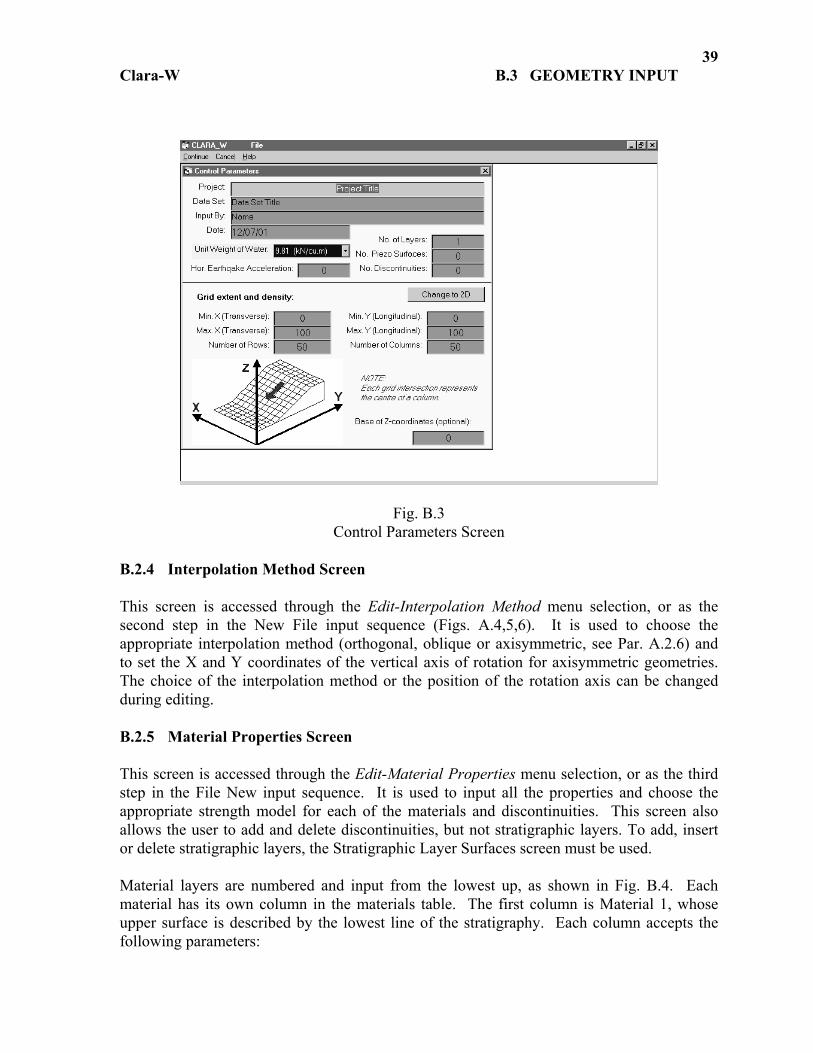
surfaces were input in the *.GRD format). Note that in the Edit Cross-sections screen, the user is responsible for inputting the data for all the cross-sections by toggling between them. The sequence will not lead the user through each cross-section. After finishing the last input screen in the sequence, CLARA-W returns to the main screen. Each screen forming the sequence can be re-visited individually through the Main Menu system to allow for editing of various parameters. The individual screens are described in detail in the following paragraphs: Each of the screens in the sequence has a Continue and Cancel option in its menu. The Continue option is used to store all the input information in the memory and move to the next screen in the sequence (or back to the Main Menu, if the screen was accessed individually). The Cancel option will cause the program to either return to the main screen without saving any modifications or to exit the New File sequence. B.2.3 Control Parameters Screen The Control Parameters screen, accessed through the Edit-Control Parameters menu selection, or appearing as the first step in the New File input sequence, is shown in Fig. B.3. It is used to name the problem file and to assign labels which will identify program output. The screen also collects information on the number of required layers and surfaces, problem boundaries, mesh spacing, earthquake acceleration and the selection of units.

Clara-W B.3 GEOMETRY INPUT
37
The following is a list of all the labels and a description of each:
- PROJECT NAME: Any alphanumeric string of any length. It may contain blanks, or remain entirely blank.
- DATA SET: Any alphanumeric string of any length. It may contain blanks, or
remain entirely blank.
- INPUT BY: The user's initials or name. May remain blank.
- DATE: taken by CLARA-W from the system calendar. It can be changed or replaced by any string.
- UNIT WEIGHT OF WATER: anticipated by CLARA-W as 9.81 (kN/m3). This
means that all subsequent input will be in terms of SI metric units: metres, kilonewtons (kN) and kilopascals (kPa). The Imperial units of feet, pounds and pounds per square foot (psf) can be selected by changing the unit weight to 62.4 (lbs/ft3).
- NUMBER OF LAYERS: specifies the number of material layers forming the
stratigraphy, including water in case of toe submergence (see Par. A.2.14). There must be at least one material layer. The maximum combined number of material and piezometric layers is 50. The maximum combined number of materials and discontinuities is also 50. NOTE: When used to edit an existing file, this screen does not allow the user to change the number of stratigraphic or piezo layers. To add, insert or delete stratigraphic layers, the Edit-Stratigraphic Layer Surfaces screen must be used.
- NUMBER OF PIEZOMETRIC SURFACES: Can be zero. Some or all of these
may eventually remain unused. The maximum combined number of material and piezometric layers is 50. For use of piezometric surfaces and other pore-water options refer to Par. A.2.13.
- NUMBER OF DISCONTINUITIES: The number of discontinuity types that the
user wishes to define (can be zero). Some or even all of these may remain unused. The maximum combined number of materials and discontinuities is 50. The use of discontinuities is described in Par. A.2.12.
- HORIZONTAL EARTHQUAKE ACCELERATION: A horizontal earthquake
acceleration for pseudo-static analysis can be entered, in terms of g units. If not required, enter 0. Eqns. 3 and 4 of Hungr et al. (1989), see Appendix A, describes the use of the coefficient in the equilibrium equations.
Clara-W B.3 GEOMETRY INPUT
38
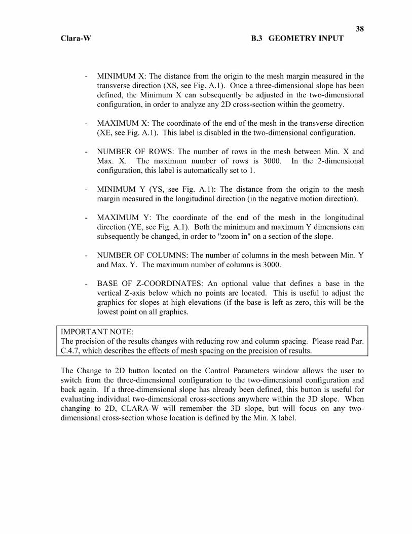
- MINIMUM X: The distance from the origin to the mesh margin measured in the transverse direction (XS, see Fig. A.1). Once a three-dimensional slope has been defined, the Minimum X can subsequently be adjusted in the two-dimensional configuration, in order to analyze any 2D cross-section within the geometry.
- MAXIMUM X: The coordinate of the end of the mesh in the transverse direction
(XE, see Fig. A.1). This label is disabled in the two-dimensional configuration.
- NUMBER OF ROWS: The number of rows in the mesh between Min. X and Max. X. The maximum number of rows is 3000. In the 2-dimensional configuration, this label is automatically set to 1.
- MINIMUM Y (YS, see Fig. A.1): The distance from the origin to the mesh
margin measured in the longitudinal direction (in the negative motion direction).
- MAXIMUM Y: The coordinate of the end of the mesh in the longitudinal direction (YE, see Fig. A.1). Both the minimum and maximum Y dimensions can subsequently be changed, in order to "zoom in" on a section of the slope.
- NUMBER OF COLUMNS: The number of columns in the mesh between Min. Y
and Max. Y. The maximum number of columns is 3000.
- BASE OF Z-COORDINATES: An optional value that defines a base in the vertical Z-axis below which no points are located. This is useful to adjust the graphics for slopes at high elevations (if the base is left as zero, this will be the lowest point on all graphics.
IMPORTANT NOTE: The precision of the results changes with reducing row and column spacing. Please read Par. C.4.7, which describes the effects of mesh spacing on the precision of results. The Change to 2D button located on the Control Parameters window allows the user to switch from the three-dimensional configuration to the two-dimensional configuration and back again. If a three-dimensional slope has already been defined, this button is useful for evaluating individual two-dimensional cross-sections anywhere within the 3D slope. When changing to 2D, CLARA-W will remember the 3D slope, but will focus on any two-dimensional cross-section whose location is defined by the Min. X label.
Clara-W B.3 GEOMETRY INPUT
39
Fig. B.3 Control Parameters Screen
B.2.4 Interpolation Method Screen This screen is accessed through the Edit-Interpolation Method menu selection, or as the second step in the New File input sequence (Figs. A.4,5,6). It is used to choose the appropriate interpolation method (orthogonal, oblique or axisymmetric, see Par. A.2.6) and to set the X and Y coordinates of the vertical axis of rotation for axisymmetric geometries. The choice of the interpolation method or the position of the rotation axis can be changed during editing. B.2.5 Material Properties Screen This screen is accessed through the Edit-Material Properties menu selection, or as the third step in the File New input sequence. It is used to input all the properties and choose the appropriate strength model for each of the materials and discontinuities. This screen also allows the user to add and delete discontinuities, but not stratigraphic layers. To add, insert or delete stratigraphic layers, the Stratigraphic Layer Surfaces screen must be used.
Material layers are numbered and input from the lowest up, as shown in Fig. B.4. Each material has its own column in the materials table. The first column is Material 1, whose upper surface is described by the lowest line of the stratigraphy. Each column accepts the following parameters:
Clara-W B.3 GEOMETRY INPUT
40
- MATERIAL IDENTIFICATION LABEL: An alphanumeric string, which can contain blanks or remain blank. Example: FIRM CLAY.
- UNIT WEIGHT: in kN/m3 or pcf (disabled for discontinuities).
- STRENGTH PROPERTIES: CLARA-W uses three alternative material strength
models (described in Appendix C). Depending on the choice of model, certain fields in the column become yellow, which means that they are inaccessible for editing:
1) Coulomb Isotropic Model: The standard linear strength model described
by a single pair of friction angles (in degrees) and cohesion values.
2) Coulomb Anisotropic Model: Described by two friction angles (in degrees), one for horizontal planes and another for vertical. Similarly, there are two cohesion values. The actual friction angle and cohesion used in each column will depend on the local dip of the sliding surface.
3) Non-Linear Model: Described by four parameters: A,B,D and Uniaxial
Compressive Strength. An apparent friction angle and cohesion is derived from these in each iteration depending on the normal effective stress.
- Two special types of material are described as follows:
1) Water: this material has no strength and no editing of the properties is
possible.
2) Hard Layer: Specifying a certain material layer as a hard layer will force all sliding surfaces to pass just above the top surface of the hard layer, as described in Par. A.2.8.
- PIEZOMETRIC SURFACE: This field allows for the specification of the
piezometric surface associated with each material or discontinuity. The three possible ways to specify the pore-pressure conditions are described in Par. A.2.13 and in Fig. A.16.
- PORE-PRESSURE RATIO (ru): As an alternative to a Piezo Surface, the pore-
pressure in a layer or discontinuity can be specified by a pore-pressure ratio (Par. A.2.13). Each material or discontinuity can have either a piezo surface or a pore-pressure. CLARA-W will not allow both to be defined at the same time.
- B COEFFICIENT: This can only be specified for layers other than the uppermost
layer, which have a piezo surface associated with them. When a zero value is

Clara-W B.3 GEOMETRY INPUT
41
specified, there will be no excess pore-pressure. Values between 0 and 1 will result in an excess pore pressure equal to B times the total weight of the uppermost layer (fill) to be added to the piezometric pressure (see Eqn 2 and Fig. A.16).
Fig. B.4 Material and Discontinuity Properties Definition Screen.
B.2.6 Discontinuity Properties The definition of discontinuity properties is the same as for a Material, except that Unit Weight is not needed (see Fig. B.4). The discontinuities will be associated with parts of the sliding surface, by methods described in Par. C.2.7. B.2.7 Stratigraphic Layer Surfaces Screen This screen is accessed through the Edit-Stratigraphic Layers menu selection, or as the fourth step in the New File input sequence (Fig. B.5). It is used to determine the type of input surface used for each layer. The choices are: cross-section based input, *.GRD file and at-constant depth, as described in Par. A.2.4. This screen also allows the user to add, insert or delete stratigraphic layers.
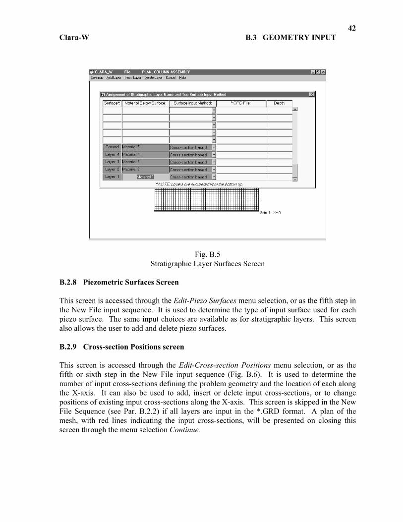
Clara-W B.3 GEOMETRY INPUT
42
Fig. B.5 Stratigraphic Layer Surfaces Screen
B.2.8 Piezometric Surfaces Screen This screen is accessed through the Edit-Piezo Surfaces menu selection, or as the fifth step in the New File input sequence. It is used to determine the type of input surface used for each piezo surface. The same input choices are available as for stratigraphic layers. This screen also allows the user to add and delete piezo surfaces. B.2.9 Cross-section Positions screen This screen is accessed through the Edit-Cross-section Positions menu selection, or as the fifth or sixth step in the New File input sequence (Fig. B.6). It is used to determine the number of input cross-sections defining the problem geometry and the location of each along the X-axis. It can also be used to add, insert or delete input cross-sections, or to change positions of existing input cross-sections along the X-axis. This screen is skipped in the New File Sequence (see Par. B.2.2) if all layers are input in the *.GRD format. A plan of the mesh, with red lines indicating the input cross-sections, will be presented on closing this screen through the menu selection Continue.

Clara-W B.3 GEOMETRY INPUT
43
Fig. B.6 Cross-section Positions Screen
B.3 GEOMETRY INPUT B.3.1 Edit Cross-sections Screen This screen is accessed through the Edit-Cross-sections menu selection, or as the sixth or seventh step in the New File input sequence, and is the last part of the Input Sequence (Fig. B.7). It is used to input or edit the data for each cross-section graphically or numerically. It is skipped in the New File Sequence (see Par. B.2.2) if all layers are input in the *.GRD format. In this screen, the problem geometry is entered or modified as a sequence of input cross-sections whose positions are defined in the Cross-Section Positions screen (refer to Par. B.2.9). The preparation of the data for input is described in Par. B.2.1. The user can toggle between sections by pressing the Section Number button, and between lines by pressing the Layer No. button on the data table. Alternatively, the user can go directly to a different layer or section using the appropriate menu entry. Each cross-section is input in succession, always beginning with Cross-Section 1. Each layer is drawn on the screen as a series of points, input graphically or numerically and connected by a line. The layers are selected and input or modified one at a time. The currently selected
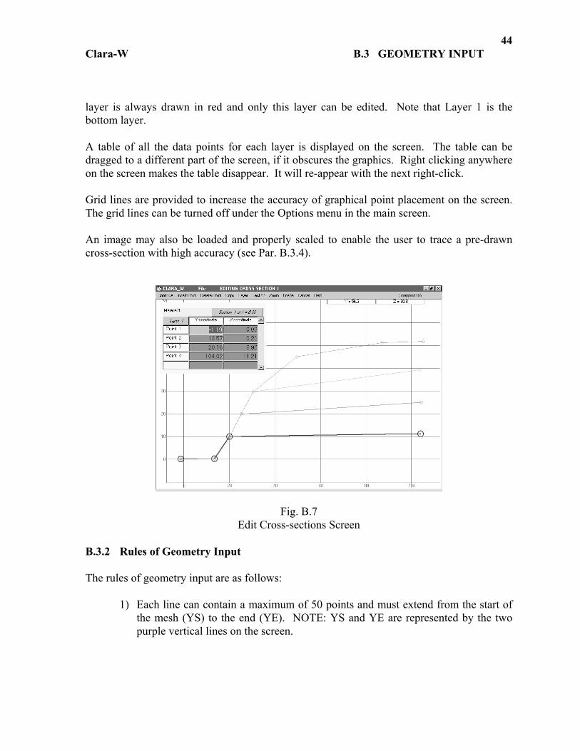
Clara-W B.3 GEOMETRY INPUT
44
layer is always drawn in red and only this layer can be edited. Note that Layer 1 is the bottom layer. A table of all the data points for each layer is displayed on the screen. The table can be dragged to a different part of the screen, if it obscures the graphics. Right clicking anywhere on the screen makes the table disappear. It will re-appear with the next right-click. Grid lines are provided to increase the accuracy of graphical point placement on the screen. The grid lines can be turned off under the Options menu in the main screen. An image may also be loaded and properly scaled to enable the user to trace a pre-drawn cross-section with high accuracy (see Par. B.3.4).
Fig. B.7 Edit Cross-sections Screen
B.3.2 Rules of Geometry Input The rules of geometry input are as follows:
1) Each line can contain a maximum of 50 points and must extend from the start of the mesh (YS) to the end (YE). NOTE: YS and YE are represented by the two purple vertical lines on the screen.

Clara-W B.3 GEOMETRY INPUT
45
2) Lines may touch, or join and travel together. However, to avoid conflict, lines that cross each other will be automatically adjusted once the screen is closed. This does not apply for Piezometric surfaces, which may cross other layers.
IMPORTANT: Adjustment to eliminate lines-crossing conflict. Wherever a lower line in the stratigraphic succession projects above an upper line, the upper line will be brought down to the level of the lower line. Clara-W will issue a warning message: "Line crossing conflict has been corrected by adjusting Surface 1". Note that by purposely drawing the highest stratigraphic line so as to intersect lower lines, one can conveniently simulate the effect of an excavation. The warning is issued each time the problem geometry is recompiled.
3) CLARA-W will not tolerate negatively sloping lines. Therefore, clicking to the
left of the last entered point will have no effect (although it is possible to insert points using the menu, see Par. B.3.3).
4) When the next cross-section is selected, all data input for the previous section will
be entered in the memory. NOTE: The Cancel option on the menu only cancels data input for the current section.
B.3.3 How to Input/Edit Cross-Section Geometry The following is a list of the functions available in the Edit Cross-Sections screen:
- ADDING AND INSERTING POINTS: Points may be added graphically by
clicking in the appropriate place on the screen to the right of any previous points. Points can also be added numerically by entering the coordinates in the table. Inserting a point may be done by choosing the Insert Point option in the menu and then clicking in either the appropriate place on the screen, or on the appropriate line in the data table. After selecting the Insert Point option, the action may be canceled by clicking the Cancel button in the lower left corner of the screen.
- DELETING POINTS: Points may be deleted by selecting the Delete Point option
in the menu and then clicking on either the appropriate point on the screen, or on the appropriate line in the data table. Pressing the cancel button on the lower left corner of the screen will cancel the action.
- SNAP OPTION: The Snapping feature, which is turned on by default, causes a
point that is drawn near enough to another point, located either on the line immediately below or above the current line, to snap to the other point's exact location. This feature may be turned off by clicking the option on the far right of the menu bar.
Clara-W B.3 GEOMETRY INPUT
46
- MOVING LINE CLUSTERS: When a point containing more than one line is
moved, all points on other lines with exactly the same coordinates will be moved with it. This can considerably speed up the editing of a geometry. This feature can be turned off or on by toggling the "Clusters on/off" entry on the Edit-cross-sections screen menu. Please remember that points will only form clusters if drawn with the "Snapping on" feature. Without it, the point coordinates may not be exactly identical and the points may thus not be recognized as part of a cluster.
- LINE SLOPE: When an existing geometry point is clicked in the Edit-cross-
sections screen, in order to be moved, CLARA-W will show a label on which the slope of the line segment immediately to the left is displayed. This will aid in constructing slopes of known inclination. The format of the label is "1 vertical : x horizontal" (example, 1 : 2.5).
- COPY ABOVE / COPY BELOW: The Copy Above option under the Copy menu
allows the user to copy the next point to the right on the layer above the current one. This function is disabled if there is no layer above the current one. The Copy Below option works identically to the Copy Above option except that it copies the point on the layer below the current layer. These functions can be operated from the keyboard by pressing Ctrl+A or Ctrl+B. This allows for a rapid input of long lines identical to other lines already present.
- COPY LAYER: The Copy Layer option under the Copy menu allows the user to
copy any layer already entered in the section. Note that all previous points on the current layer will be replaced by the copied points.
- COPY SECTION: The Copy Section option under the Copy menu allows the user
to replace all the points in all the layers and piezo surfaces of the current cross-section with those of any other section. NOTE: This option must be used carefully, as there is no Undo function.
- MOVING BETWEEN LAYERS: By choosing the appropriate layer under the
Layer menu, another layer in a cross-section can be selected. Alternatively, by clicking the command button on the data table displaying the current layer or piezo number, it is possible to toggle to the next layer.
- MOVING BETWEEN SECTIONS: By choosing the appropriate section under
the Section menu, it is possible to move to another cross-section. Alternatively, by clicking the command button on the data table, it is possible to toggle to the next section. The data table displays the current section and its X-coordinate. Note that all the points in the current section will be stored in the memory as soon as another cross-section is loaded.
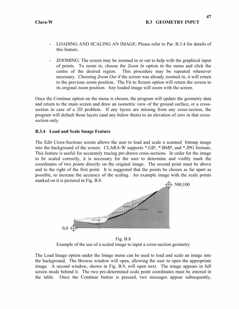
Clara-W B.3 GEOMETRY INPUT
47
- LOADING AND SCALING AN IMAGE: Please refer to Par. B.3.4 for details of this feature.
- ZOOMING: The screen may be zoomed in or out to help with the graphical input
of points. To zoom in, choose the Zoom In option in the menu and click the centre of the desired region. This procedure may be repeated whenever necessary. Choosing Zoom Out if the screen was already zoomed in, it will return to the previous zoom position. The Fit to Screen option will return the screen to its original zoom position. Any loaded image will zoom with the screen.
Once the Continue option on the menu is chosen, the program will update the geometry data and return to the main screen and draw an isometric view of the ground surface, or a cross-section in case of a 2D problem. If any layers are missing from any cross-section, the program will default those layers (and any below them) to an elevation of zero in that cross-section only. B.3.4 Load and Scale Image Feature The Edit Cross-Sections screen allows the user to load and scale a scanned bitmap image into the background of the screen. CLARA-W supports *.GIF, *.BMP, and *.JPG formats. This feature is useful for accurately tracing pre-drawn cross-sections. In order for the image to be scaled correctly, it is necessary for the user to determine and visibly mark the coordinates of two points directly on the original image. The second point must be above and to the right of the first point. It is suggested that the points be chosen as far apart as possible, to increase the accuracy of the scaling. An example image with the scale points marked on it is pictured in Fig. B.8.
Fig. B.8 Example of the use of a scaled image to input a cross-section geometry
The Load Image option under the Image menu can be used to load and scale an image into the background. The Browse window will open, allowing the user to open the appropriate image. A second window, shown in Fig. B.9, will open next. The image appears in full screen mode behind it. The two pre-determined scale point coordinates must be entered in the table. Once the Continue button is pressed, two messages appear subsequently,
0,0
500,100
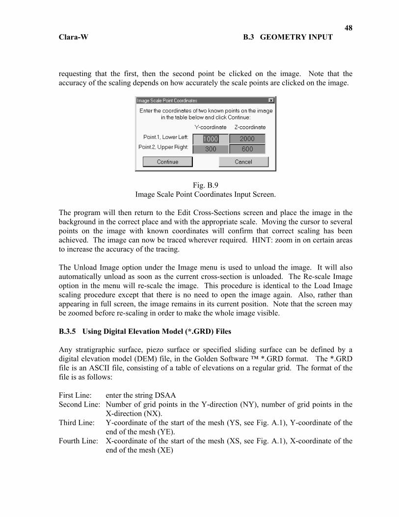
Clara-W B.3 GEOMETRY INPUT
48
requesting that the first, then the second point be clicked on the image. Note that the accuracy of the scaling depends on how accurately the scale points are clicked on the image.
Fig. B.9 Image Scale Point Coordinates Input Screen.
The program will then return to the Edit Cross-Sections screen and place the image in the background in the correct place and with the appropriate scale. Moving the cursor to several points on the image with known coordinates will confirm that correct scaling has been achieved. The image can now be traced wherever required. HINT: zoom in on certain areas to increase the accuracy of the tracing. The Unload Image option under the Image menu is used to unload the image. It will also automatically unload as soon as the current cross-section is unloaded. The Re-scale Image option in the menu will re-scale the image. This procedure is identical to the Load Image scaling procedure except that there is no need to open the image again. Also, rather than appearing in full screen, the image remains in its current position. Note that the screen may be zoomed before re-scaling in order to make the whole image visible. B.3.5 Using Digital Elevation Model (*.GRD) Files Any stratigraphic surface, piezo surface or specified sliding surface can be defined by a digital elevation model (DEM) file, in the Golden Software ™ *.GRD format. The *.GRD file is an ASCII file, consisting of a table of elevations on a regular grid. The format of the file is as follows: First Line: enter the string DSAA Second Line: Number of grid points in the Y-direction (NY), number of grid points in the
X-direction (NX). Third Line: Y-coordinate of the start of the mesh (YS, see Fig. A.1), Y-coordinate of the
end of the mesh (YE). Fourth Line: X-coordinate of the start of the mesh (XS, see Fig. A.1), X-coordinate of the
end of the mesh (XE)

Clara-W B.3 GEOMETRY INPUT
49
Subsequent Lines: Rows of elevation values. Each row is NY members long and there are NX rows. Thus, the values represent points increasing in the y-direction, then in X-direction.
An example of the first six lines of a *.GRD file follows: DSAA 71 127 0 350 0 630 141.818 273.535 177.218 177.779 178.438 179.197 180.389 181.733 183.027 184.376 185.815 NOTE: If creating the *.GRD file by Golden Software SURFER ™ program, remember that the SURFER X-coordinate will be the Y-coordinate in CLARA-W. The *.GRD file must be saved in the ASSCII format, as CLARA-W will not read a binary file. If any surface in a problem is specified as a *.GRD surface, the control parameters NX, NY, XS,XE, YS and YE, defining the extent and density of the mesh, will automatically be set to those specified by the *.GRD file. The control parameters cannot then be changed. Cross-section input or at-constant depth input can be used in combination with a *.GRD file, to define surfaces below those specified by the *.GRD file. An example file using a DEM is given in Example 10, Part D.

50
______________________________
PART C
SLOPE STABILITY ANALYSIS
_____________________________

Clara-W C.2 DEFINITION OF SLIDING SURFACES AND SEARCHES
51
C.1 ANALYSIS OPTIONS C.1.1 General The general procedure for producing slope stability solutions is as follows:
1) Assemble the problem geometry and material/discontinuity properties, as
described in Section B. 2) Define a single sliding surface (ellipsoid, compound, wedge or general), or search
(automatic or grid) as described in Section C.2. When this is completed, a graphical representation of the sliding surface will appear on the screen. This will be either an isometric view for a 3D problem, or a section for a 2D problem. The Solve menu selection will now become enabled.
3) Define solution options (earthquake acceleration, external forces, tension crack or angle of rotation).
4) Select Solve, with the appropriate surface or search. 5) Print out or export a table of results and graphics.
C.1.2 Earthquake Acceleration A horizontal earthquake acceleration for pseudo-static analysis can be entered in terms of g units. Hungr et al. (1989) in Appendix A (Eqns 3 and 4) describes the use of this coefficient in the equilibrium equations. C.1.3 External Forces Screen This screen is accessed through the Edit-External Forces menu selection (Fig. C.1). It is used to define the application coordinates and the vertical and horizontal components of any external forces acting on the surface. This screen also allows the user to add and delete external forces. C.1.4 Tension Crack Screen This screen is accessed through the Edit-Tension Crack menu selection (Fig. C.2). It is used to input a tension crack as described in Par. A.2.9. The tension crack can be specified by a Y-coordinate where it is located. Alternatively, if the depth of the tension crack is specified, it will be moved to an appropriate Y-coordinate so that the specified depth results in the cross-section central to the current mesh (i.e. in the longitudinal section located at an X-coordinate which is an average of XS and XE). The percentage filling of the tension crack by water will also be specified (see Par. A.2.9). NOTE: if the percentage filling is zero, no tension crack water thrust will be generated.

Clara-W C.2 DEFINITION OF SLIDING SURFACES AND SEARCHES
52
Fig. C.1
External Forces Screen
Fig. C.2
Tension Crack Screen

Clara-W C.2 DEFINITION OF SLIDING SURFACES AND SEARCHES
53
C.1.5 Rotation of the Reference Frame CLARA-W resolves the equations of equilibrium in the direction of the Y-coordinate axis. Therefore, the direction of sliding must be pre-determined when the coordinate axes and the mesh are set (see Par. B.2.1). A feature has been provided which allows the direction of resolution to be changed by several degrees, positively and negatively, without changing the mesh. The rotation angle is set through the Solve-Rotation Angle selection in the main menu. The rotation angle θ can be set only for the analysis of a single sliding surface, using the Bishop or Janbu Methods. It cannot be used with searches, or with the Spencer or Morgenstern-Price methods. The rotation angle is set for one analysis only, then re-set automatically to zero. The solution technique consists of finding slope angles at the base of each column, perpendicular and parallel to the chosen perturbation direction. The external horizontal loads and water forces are reduced by the cosine of the rotation angle. The solution is then carried out in the usual way. The new slope angles are calculated as follows:
)costansinarctan(tan' θαθαα yxy += Eqn.[3]
)]2/cos(tan)2/sin(arctan[tan' πθαπθαα +++= yxx Eqn.[4] Here, αx and αy are the slope angles of the sliding surface perpendicular and parallel with the sliding direction respectively. IMPORTANT: The rotation feature may not be able to correct the situation if the mesh directions do not correspond to kinematically-favourable movement directions. C.2 DEFINITION OF SLIDING SURFACES AND SEARCHES C.2.1 Input of a Single Ellipsoidal Sliding Surface The types of sliding surfaces are described in Par. A.2.7. The input screen for an Ellipsoidal Sliding Surface is shown in Fig. C.3. The position of the ellipsoid center and the tangent plane elevation may be input numerically in the table or graphically by dragging the dark green square handles on the main screen. The X-coordinate of the centre and the Aspect Ratio can only be entered numerically in the table. The screen can also be zoomed in or out as required. When the Continue option on the menu is chosen, the program returns to the main screen and draws an isometric view of the sliding surface (or a cross-section, if two-dimensional). Also the Single Trial Surface option under the Solve menu is enabled. This allows the user to solve the surface.
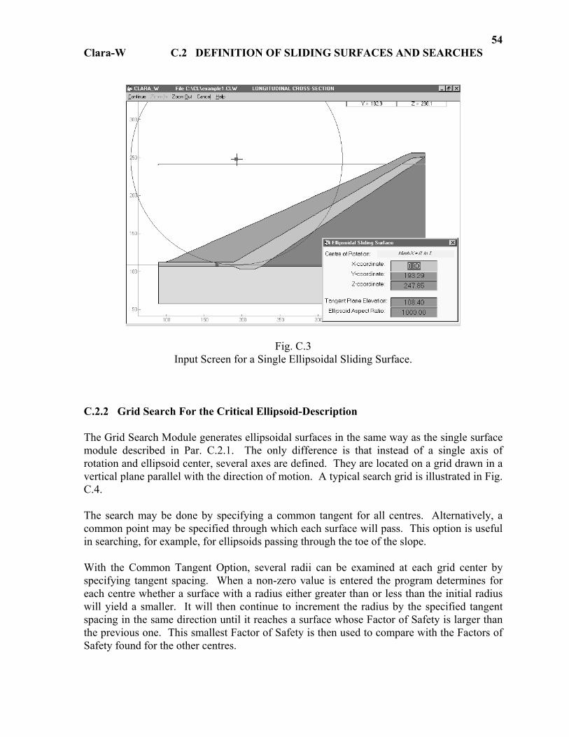
Clara-W C.2 DEFINITION OF SLIDING SURFACES AND SEARCHES
54
Fig. C.3 Input Screen for a Single Ellipsoidal Sliding Surface.
C.2.2 Grid Search For the Critical Ellipsoid-Description The Grid Search Module generates ellipsoidal surfaces in the same way as the single surface module described in Par. C.2.1. The only difference is that instead of a single axis of rotation and ellipsoid center, several axes are defined. They are located on a grid drawn in a vertical plane parallel with the direction of motion. A typical search grid is illustrated in Fig. C.4. The search may be done by specifying a common tangent for all centres. Alternatively, a common point may be specified through which each surface will pass. This option is useful in searching, for example, for ellipsoids passing through the toe of the slope. With the Common Tangent Option, several radii can be examined at each grid center by specifying tangent spacing. When a non-zero value is entered the program determines for each centre whether a surface with a radius either greater than or less than the initial radius will yield a smaller. It will then continue to increment the radius by the specified tangent spacing in the same direction until it reaches a surface whose Factor of Safety is larger than the previous one. This smallest Factor of Safety is then used to compare with the Factors of Safety found for the other centres.
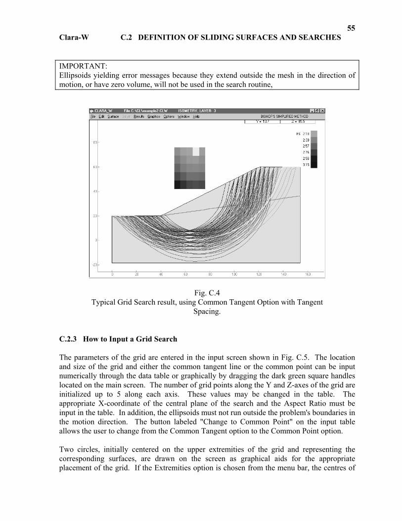
Clara-W C.2 DEFINITION OF SLIDING SURFACES AND SEARCHES
55
IMPORTANT: Ellipsoids yielding error messages because they extend outside the mesh in the direction of motion, or have zero volume, will not be used in the search routine,
Fig. C.4 Typical Grid Search result, using Common Tangent Option with Tangent
Spacing.
C.2.3 How to Input a Grid Search The parameters of the grid are entered in the input screen shown in Fig. C.5. The location and size of the grid and either the common tangent line or the common point can be input numerically through the data table or graphically by dragging the dark green square handles located on the main screen. The number of grid points along the Y and Z-axes of the grid are initialized up to 5 along each axis. These values may be changed in the table. The appropriate X-coordinate of the central plane of the search and the Aspect Ratio must be input in the table. In addition, the ellipsoids must not run outside the problem's boundaries in the motion direction. The button labeled "Change to Common Point" on the input table allows the user to change from the Common Tangent option to the Common Point option. Two circles, initially centered on the upper extremities of the grid and representing the corresponding surfaces, are drawn on the screen as graphical aids for the appropriate placement of the grid. If the Extremities option is chosen from the menu bar, the centres of

Clara-W C.2 DEFINITION OF SLIDING SURFACES AND SEARCHES
56
the two circles are changed to the lower extremities of the grid. The screen may be zoomed in or out using the Zoom options on the menu bar. Once the input screen is complete, the Continue option on the menu bar returns the user to the main screen. The initial trial surface will be shown graphically. The Grid Search option under the Solve menu will now be enabled. Once clicked, the program will begin the Grid Search solution routine (see Par. C.2.6). In general, it will be necessary to repeat the search for several Aspect Ratios in order to find the smallest Factor of Safety.
Fig. C.5 Grid Search Input Screen.
C.2.4 Automatic Search For the Critical Ellipsoid-Description The Automatic Search works similarly to the Grid Search. Ellipsoidal surfaces are generated with centres lying in a vertical plane parallel to the direction of motion. The method of searching is shown in Fig. C.6. An initial center of rotation and grid spacing are specified. Eight centres surrounding the initial one are tested and the one with the least Factor of Safety is chosen as the center of the next grid. The search ceases when a point is found surrounded by 8 higher safety factors. The function of tangent plane spacing is as described in Par. C.2.2.
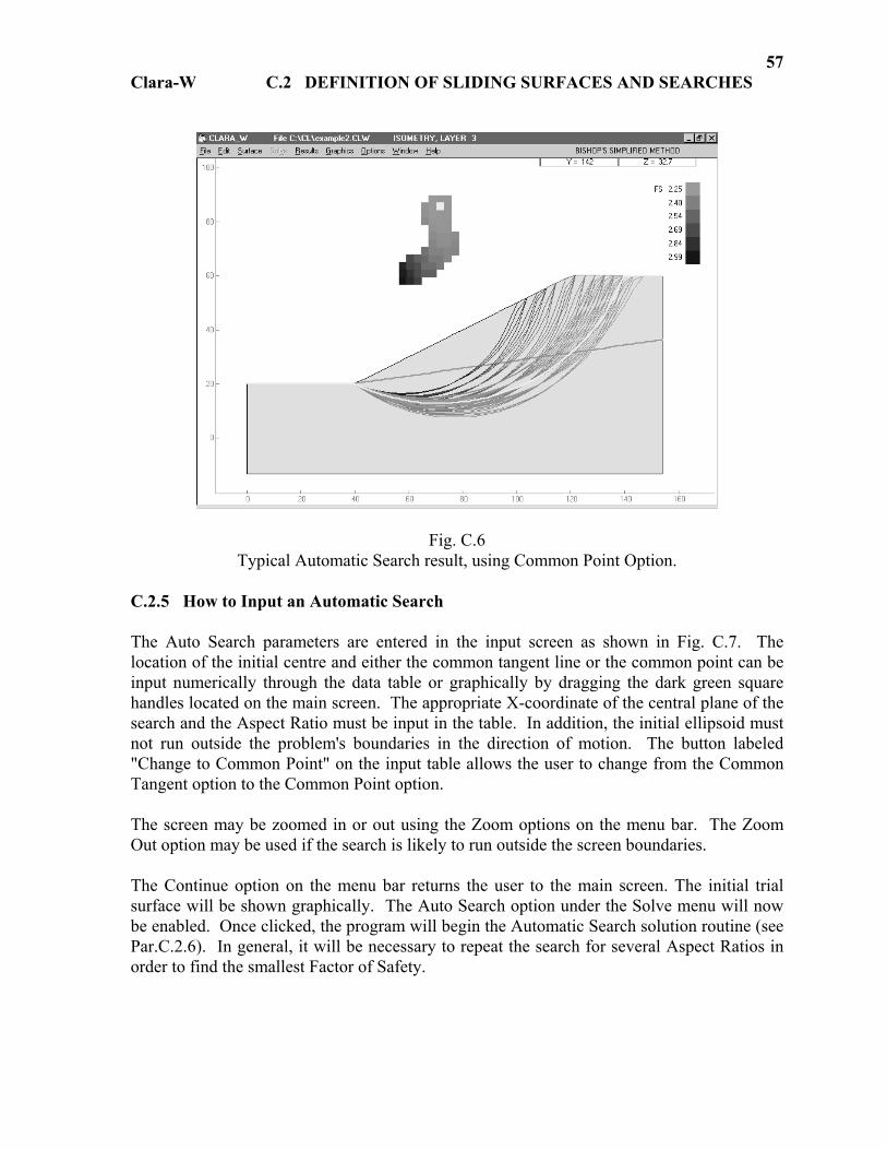
Clara-W C.2 DEFINITION OF SLIDING SURFACES AND SEARCHES
57
Fig. C.6 Typical Automatic Search result, using Common Point Option.
C.2.5 How to Input an Automatic Search The Auto Search parameters are entered in the input screen as shown in Fig. C.7. The location of the initial centre and either the common tangent line or the common point can be input numerically through the data table or graphically by dragging the dark green square handles located on the main screen. The appropriate X-coordinate of the central plane of the search and the Aspect Ratio must be input in the table. In addition, the initial ellipsoid must not run outside the problem's boundaries in the direction of motion. The button labeled "Change to Common Point" on the input table allows the user to change from the Common Tangent option to the Common Point option. The screen may be zoomed in or out using the Zoom options on the menu bar. The Zoom Out option may be used if the search is likely to run outside the screen boundaries. The Continue option on the menu bar returns the user to the main screen. The initial trial surface will be shown graphically. The Auto Search option under the Solve menu will now be enabled. Once clicked, the program will begin the Automatic Search solution routine (see Par.C.2.6). In general, it will be necessary to repeat the search for several Aspect Ratios in order to find the smallest Factor of Safety.

Clara-W C.2 DEFINITION OF SLIDING SURFACES AND SEARCHES
58
Fig. C.7 Automatic Search Input Screen.
C.2.6 Grid Search and Auto Search Solution Screens Once the Grid Search or Auto Search Input screen has been completed, the first trial sliding surface will be shown in isometry or section on the screen and the corresponding option under the Solve menu will be enabled. This option begins the search solution routine. As the routine proceeds, all tested surfaces are drawn on the screen in the appropriate colour scheme. The resulting critical surface is drawn in yellow. While the search is running, the Information Window shown in Fig. C.8 (which can be dragged across the screen), displays some of the output results for each corresponding surface. After the search is completed, the window displays the output for the Critical Surface. During execution, the search may be paused by clicking the Pause button in the Information Window. The user may then either continue or exit the search. Once a Critical Surface is found, the caption on the Pause button changes to "Tentative Critical Surface." This button now calls up the Plan of Active Columns screen for this Critical Surface. IMPORTANT: The sliding surface resulting from the automatic search must only be regarded as a first approximation of the "critical" surface. For an accurate result, several automatic and grid searches should be combined, each with different starting points. The user should also exercise experienced judgment in selecting the critical surface according to the stratigraphic conditions and structure of the slope.

Clara-W C.2 DEFINITION OF SLIDING SURFACES AND SEARCHES
59
Fig. C.8 Grid and Automatic Search Information Window.
C.2.7 Input of a Multi-Planar Wedge Surface Each line in the input table shown in Fig. C.9 describes one of the component planes by means of a reference point, dip angle and dip direction (with respect to the direction of sliding: positive clockwise). The reference point is any point in space lying on the plane, inside or outside the slide area. Each plane has an associated discontinuity code number referring to a defined discontinuity type. If this number is zero, the properties of that plane will be taken from the material stratigraphy. Planes may be added either by choosing the Add Plane option from the menu or by moving the cursor down to the next empty line. The Delete Plane option in the menu will delete the line on which the cursor is currently placed. The method for assembling the sliding surface is described in Par. A.2.7. The user is responsible for choosing plane combinations which will yield a kinematically feasible slide. IMPORTANT: CLARA-W is less suited to classical wedge solutions than rigid-body wedge programs and should not be extensively used for these surfaces. C.2.8 Input of a General Sliding Surface The input is initiated by the screen shown in Fig. C.10. The General Surface may be cross-section based or it may be loaded from a *.GRD Grid File. The combo box on the input table offers both choices. When the Grid File option is chosen, the Browse window opens, thus allowing the user to choose the appropriate *.GRD file. Once loaded, the path and file name will be displayed in the cell adjacent to the above mentioned combo box. The file may be changed by clicking
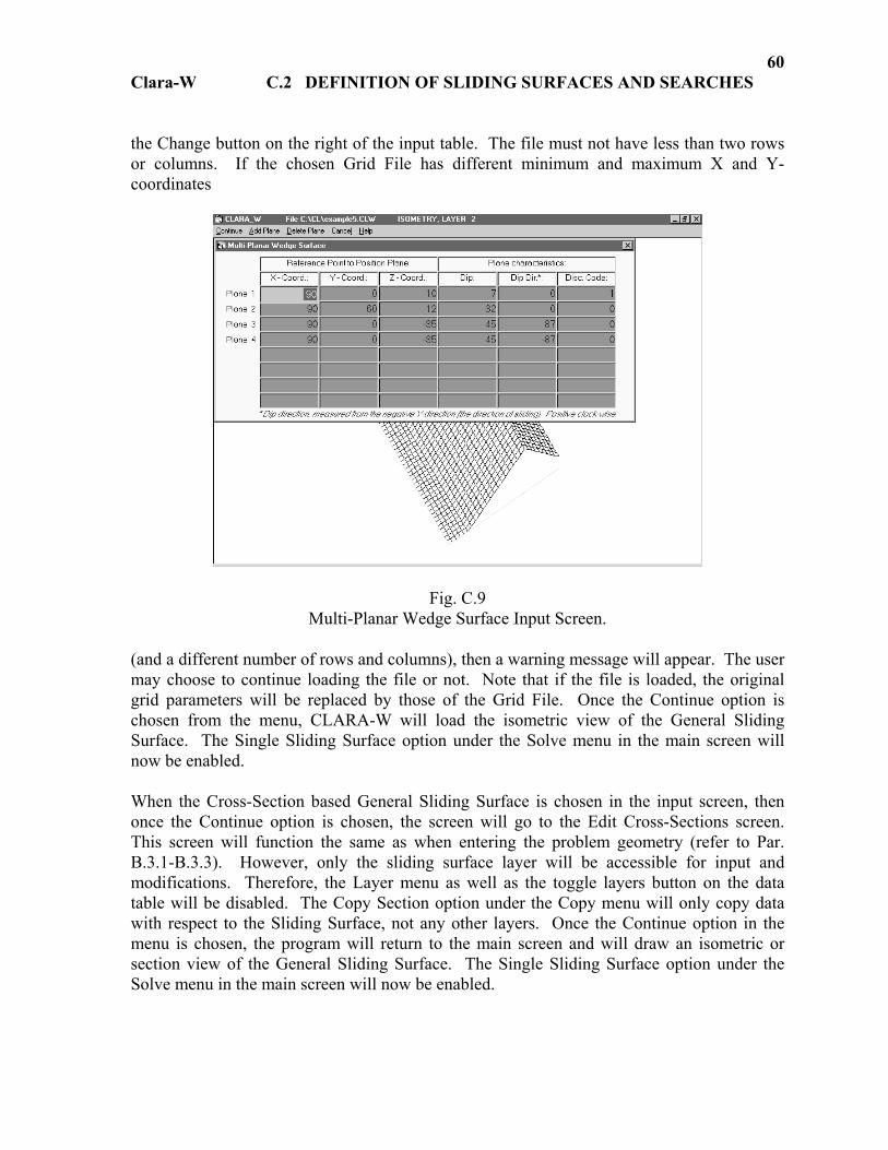
Clara-W C.2 DEFINITION OF SLIDING SURFACES AND SEARCHES
60
the Change button on the right of the input table. The file must not have less than two rows or columns. If the chosen Grid File has different minimum and maximum X and Y-coordinates
Fig. C.9 Multi-Planar Wedge Surface Input Screen.
(and a different number of rows and columns), then a warning message will appear. The user may choose to continue loading the file or not. Note that if the file is loaded, the original grid parameters will be replaced by those of the Grid File. Once the Continue option is chosen from the menu, CLARA-W will load the isometric view of the General Sliding Surface. The Single Sliding Surface option under the Solve menu in the main screen will now be enabled. When the Cross-Section based General Sliding Surface is chosen in the input screen, then once the Continue option is chosen, the screen will go to the Edit Cross-Sections screen. This screen will function the same as when entering the problem geometry (refer to Par. B.3.1-B.3.3). However, only the sliding surface layer will be accessible for input and modifications. Therefore, the Layer menu as well as the toggle layers button on the data table will be disabled. The Copy Section option under the Copy menu will only copy data with respect to the Sliding Surface, not any other layers. Once the Continue option in the menu is chosen, the program will return to the main screen and will draw an isometric or section view of the General Sliding Surface. The Single Sliding Surface option under the Solve menu in the main screen will now be enabled.

Clara-W C.2 DEFINITION OF SLIDING SURFACES AND SEARCHES
61
The Continue option in the menu will return the program to the main screen and display the sliding surface. The Single Trial Surface option under the Solve menu will now be enabled. Interpolation between cross-sections will be done by means of orthogonal interpolation. NOTE: This sliding surface option cannot be used with the oblique or axisymmetric interpolation methods. Should the user accidentally enter points so that a part of the sliding surface extends above the ground, the solver routine will make this part coincide with the slope surface. The general sliding surface geometry is recorded in the problem file.
Fig. C.10 General Sliding Surface Input Screen.
“FIELDS” OPTION for general sliding surfaces: The strength parameters used by a general (cross-section-specified) sliding surface are normally set according to the position of the sliding surface within the stratigraphy. With the Fields Option, it is possible to over-ride the strength (and groundwater) properties within a rectangular field defined on the plan of the column assembly. To invoke this option, follow this procedure: - Select “sliding surface-general”. - In the “general surface” screen, select “Set Discontinuity Field”.

Clara-W C.2 DEFINITION OF SLIDING SURFACES AND SEARCHES
62
- The discontinuity field screen will appear as depicted in Figure C11. -Note: At least one discontinuity must be defined. The field will always take the
properties of Discontinuity #1. - IMPORTANT: The parameters defining the field boundaries are not recorded in the
project file. They must be re-set every time the general sliding surface is defined or re-defined. Please confirm correct assignment of the strength and groundwater parameters using detailed column output (p. 70 of the Manual).
- An example, a 3D model of the 1963 Vaiont Slide, is included among the Tutorial
Examples. The example should yield a Factor of Safety of 1.00 with the Morgenstern-Price method, provided that a field is set with the coordinates x=0 to 1300 and y=0 to 2000 (Figure C12). (Note: Stratigraphy Layer 1 is defined by the Vaiont-Ground-Surface.grd file. Layer 2 (“ground” by the Vaiont-Lake.grd file).
Figure C11: The new “set discontinuity field” screen
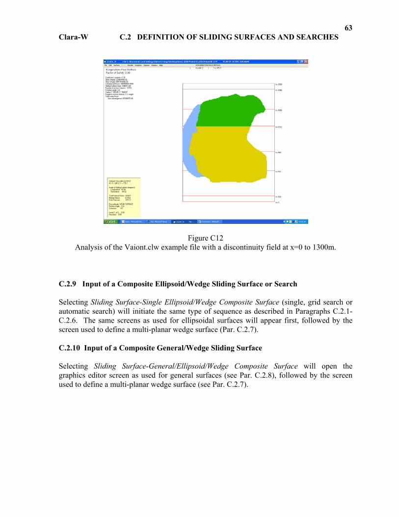
Clara-W C.2 DEFINITION OF SLIDING SURFACES AND SEARCHES
63
Figure C12 Analysis of the Vaiont.clw example file with a discontinuity field at x=0 to 1300m.
C.2.9 Input of a Composite Ellipsoid/Wedge Sliding Surface or Search Selecting Sliding Surface-Single Ellipsoid/Wedge Composite Surface (single, grid search or automatic search) will initiate the same type of sequence as described in Paragraphs C.2.1-C.2.6. The same screens as used for ellipsoidal surfaces will appear first, followed by the screen used to define a multi-planar wedge surface (Par. C.2.7). C.2.10 Input of a Composite General/Wedge Sliding Surface Selecting Sliding Surface-General/Ellipsoid/Wedge Composite Surface will open the graphics editor screen as used for general surfaces (see Par. C.2.8), followed by the screen used to define a multi-planar wedge surface (see Par. C.2.7).

Clara-W C.3 PROGRAM OPTIONS
64
C.3 PROGRAM OPTIONS C.3.1 Grid Option The Grid option under the Options menu in the main screen turns the grid lines in the Edit Cross-Sections screen on or off. The grid is initially turned on by default. Once turned off, the grid lines disappear and are replaced by a ruler-type scale running along the left and bottom edges of the screen. C.3.2 Graphics Options When Graphics Options is selected from the Options menu in the main screen, the window shown in Fig. C.11 appears. This window allows the user to change the Vertical Exaggeration Ratio, the fill style in the section drawings and the Rotation Angle for the isometry. These three options are described below:
- VERTICAL EXAGGERATION RATIO: This is the ratio between the vertical (z-
axis) and horizontal (x and y-axis) scales. A ratio of 1 signifies equal scales. A ratio greater than 1 specifies vertical exaggeration. This ratio is useful in a problem, for example, whose geometry is defined by long horizontal distances but comparatively small elevation changes. This ratio is also useful when creating the geometry cross-sections. It allows the scale in the Edit Cross-Sections screen to be stretched or shrunk in case the geometry does not fit in the default scale. NOTE: The Vertical Exaggeration Ratio must not be less than 0.
- FILL STYLE: The user may choose from three fill styles for all the Longitudinal
and Lateral Cross-Section drawings. Each layer can be drawn either in full colour, with vertical hatching, or with lines and no fill. Each layer will be drawn and filled with its corresponding colour chosen in the Colour Editor (see Par. C.3.3).
- ISOMETRY ROTATION ANGLE: The standard orientation of the isometric
plots is: Y-axis 30º up from the horizontal, X-axis at a right angle from that and Z-axis vertical. The Graphics Options window permits the user to change the angle between the Y-axis and the horizontal. The specified angle should be between 0º (side view) and 90º (front view).

Clara-W C.3 PROGRAM OPTIONS
65
Fig. C.11 Graphics Options Window.
C.3.3 Colours All surfaces and materials have different colours to help distinguish between them. The default colour for the sliding surface is purple. Piezometric surfaces are blue. The default for the selected layer in the Edit Cross-Sections screen is red. The colours of the sliding surface, the selected layer, and the first fifteen layers and piezo surfaces can be changed if desired. The Colours option under the Options menu is used to change the graphics colours. The Colour Editor, shown in Fig. C.12, will appear when this option is chosen. All the colours that may be edited are shown in the two columns on the left of the window. The colour sampler window on the upper right part of the window shows a range of colours with a certain intensity of blue. The slider, located below the sampler, can be moved to change the intensity of blue in the sampler. Once an appropriate colour has been located, it can be selected by clicking on it in the sampler. Clicking on the desired box on the left will then change its colour to the one selected. Pressing the Default button will cause the program to revert to the default colour scheme. The Save and Exit button will save the current colour scheme. This will be used in all subsequent sessions, even if the program is re-started.

Clara-W C.3 PROGRAM OPTIONS
66
Fig. C.12 Colour Editor.
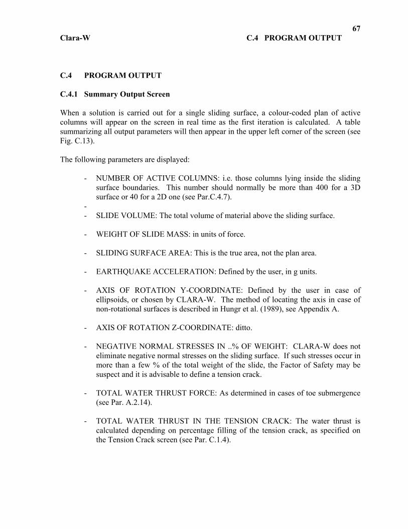
Clara-W C.4 PROGRAM OUTPUT
67
C.4 PROGRAM OUTPUT C.4.1 Summary Output Screen When a solution is carried out for a single sliding surface, a colour-coded plan of active columns will appear on the screen in real time as the first iteration is calculated. A table summarizing all output parameters will then appear in the upper left corner of the screen (see Fig. C.13). The following parameters are displayed:
- NUMBER OF ACTIVE COLUMNS: i.e. those columns lying inside the sliding
surface boundaries. This number should normally be more than 400 for a 3D surface or 40 for a 2D one (see Par.C.4.7).
- - SLIDE VOLUME: The total volume of material above the sliding surface. - WEIGHT OF SLIDE MASS: in units of force. - SLIDING SURFACE AREA: This is the true area, not the plan area. - EARTHQUAKE ACCELERATION: Defined by the user, in g units. - AXIS OF ROTATION Y-COORDINATE: Defined by the user in case of
ellipsoids, or chosen by CLARA-W. The method of locating the axis in case of non-rotational surfaces is described in Hungr et al. (1989), see Appendix A.
- AXIS OF ROTATION Z-COORDINATE: ditto.
- NEGATIVE NORMAL STRESSES IN ..% OF WEIGHT: CLARA-W does not
eliminate negative normal stresses on the sliding surface. If such stresses occur in more than a few % of the total weight of the slide, the Factor of Safety may be suspect and it is advisable to define a tension crack.
- TOTAL WATER THRUST FORCE: As determined in cases of toe submergence
(see Par. A.2.14). - TOTAL WATER THRUST IN THE TENSION CRACK: The water thrust is
calculated depending on percentage filling of the tension crack, as specified on the Tension Crack screen (see Par. C.1.4).
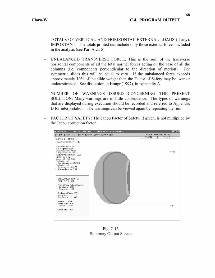
Clara-W C.4 PROGRAM OUTPUT
68
- TOTALS OF VERTICAL AND HORIZONTAL EXTERNAL LOADS (if any). IMPORTANT: The totals printed out include only those external forces included in the analysis (see Par. A.2.15)
- UNBALANCED TRANSVERSE FORCE: This is the sum of the transverse
horizontal components of all the total normal forces acting on the base of all the columns (i.e. components perpendicular to the direction of motion). For symmetric slides this will be equal to zero. If the unbalanced force exceeds approximately 10% of the slide weight then the Factor of Safety may be over or underestimated. See discussion in Hungr (1997), in Appendix A.
- NUMBER OF WARNINGS ISSUED CONCERNING THE PRESENT
SOLUTION: Many warnings are of little consequence. The types of warnings that are displayed during execution should be recorded and referred to Appendix D for interpretation. The warnings can be viewed again by repeating the run.
- FACTOR OF SAFETY: The Janbu Factor of Safety, if given, is not multiplied by
the Janbu correction factor.
Fig. C.13 Summary Output Screen
Clara-W C.4 PROGRAM OUTPUT
69
C.4.2 Error/Warning Window This window displays either a list of the data input errors or a list of the errors (if any) that occurred during the solution of a sliding surface. The list of data input errors appears before the Plan of Active Columns screen opens. If some fatal errors, such as missing material properties, are included in the list then CLARA-W will not allow a sliding surface to be solved. Instead, after this window is closed, it will return to the main screen and wait until the user corrects all the fatal errors. If no fatal errors are found, then CLARA-W will continue with the solver routine after this error window is closed. After the solver routine has completed, this window will appear again with any errors that occurred during the solution. When finished with this window, close it to continue. C.4.3 Lateral Force Balance
All existing 3D Limit Equilibrium methods, like their 2D equivalents, use only equilibrium conditions defined in the vertical plane parallel with the direction of movement. Force equilibrium in the lateral direction (horizontal, perpendicular to the direction of motion) is satisfied implicitly only in problems which are laterally symmetrical. Lateral force imbalance results from the neglect of vertical shear stresses on the lateral column boundaries. Balance can be established by imposing a suitable distribution of internal vertical shear stress, without compromising the other equilibrium conditions. Hungr et al. (1989), see Appendix A, defined an index to identify the presence of the lateral force imbalance:
WP
I hL = Eqn.[5]
Here, Ph is the resultant of the horizontal lateral components of all forces acting on the sliding body and W is the sliding body weight. This index is printed out by CLARA-W when a Bishop or Janbu analysis is carried out, and when the index value exceeds 0.01 (1%). The user is then presented with the choice to carry out a balancing procedure, as described in Par. 3.4 of Hungr (1997). IMPORTANT: If the “balanced” Factor of Safety is not significantly different from the unbalanced, the effect of lateral disequilibrium can be considered tolerable. If the two are different, then neither result should be relied on. It is sometimes possible to remove the imbalance by changing the direction in which the equilibrium equations are resolved (see Par. C.1.5). The “balanced” Factor of Safety is equivalent to the Factor of Safety that would be obtained using the method of rigid wedge analysis (see Hoek and Bray, 1977).

Clara-W C.4 PROGRAM OUTPUT
70
C.4.4 Instant Report Printable output for CLARA-W consists of a report that: outlines the results for an evaluated sliding surface, lists all the materials and discontinuities and their properties, lists all the external forces and includes a choice of graphics. The report may be previewed in CLARA-W or printed directly. It may also be saved in a *.txt file and then edited in a word processor. The Preview Report option under the Results menu in the main screen allows for a preview of the report (see Fig. C.14). A window will open requesting the user to choose which graphic is to be displayed on the report. Note that only currently displayed graphics can be used. All the currently displayed graphics are listed under the Window menu in the main screen. Once an appropriate graphic is chosen, the Continue button on the Report Graphics window will open a new window, displaying a preview of the report. If the report spans to the next page, a set of buttons with front and back arrows will appear on the top left corner of the preview window. These buttons allow the user to scroll between pages. The Print button on the top left corner will send the report to the default system printer. The Cancel button will exit the preview window without printing. Choosing the Print Report option under the Results menu in the main screen will print the report without previewing. The Report Graphics window will appear requesting the user to choose the appropriate graphic (see above paragraph). The Continue button will send the report to the default system printer. To save the report in a *.txt file, choose the Save Report in *.txt File option under the Results menu in the main screen. The Browse window will open, allowing the user to save the report in a file. Only the text in the printable report will be saved. Graphics cannot be saved in the file but may be copied to the Clipboard by either choosing the appropriate option under the Graphics menu or by pressing Ctrl+C in the main screen. The copied image may then be pasted into the saved report file using a word processor. All the lists of data, such as the list of materials and their properties, will be separated by commas. When editing the *.txt file, the "Convert text to table" function in the word processor must be used, with the commas as delimiters, to automatically place the data into tables.

Clara-W C.4 PROGRAM OUTPUT
71
Fig. C.14 Report Preview Screen
C.4.5 Detailed Output Detailed output of parameters for each individual column can be obtained by clicking the Plan of Active Columns, immediately after the analysis of a single sliding surface. The parameters displayed include:
- X and Y coordinate - ALPHA-X: The lateral inclination angle of the column base in degrees, positive
in the X-direction. - ALPHA-Y: The longitudinal inclination angle of the column base in degrees,
positive in the direction of motion (opposite to Y). - TOTAL VERTICAL STRESS: overburden pressure at the centre of the column
- TOTAL NORMAL STRESS: The total normal stress calculated at the centre of
the column base, using Equation 1 of Hungr et al. (1989), Appendix A.
Clara-W C.4 PROGRAM OUTPUT
72
- PORE-PRESSURE: The neutral (pore-water) pressure acting at the centre of the column base.
- MATERIAL/DISCONTINUITY: The material layer or discontinuity, whose
properties apply at the base of this column.
- FRICTION ANGLE: The apparent effective friction angle on the base of the column.
- C: The apparent cohesion on the column base.
- LOCAL FACTOR OF SAFETY: The ratio between available shear strength and
the shear stress at the base of the column (100 is set as a maximum, as this parameter could theoretically reach an infinite value).
C.4.6 Graphics Output Graphics generated on the screen can be output by several methods:
- Copying to the clipboard: The image on the current screen can be copied to the clipboard by choosing the appropriate option from the Graphics menu or by pressing Ctrl+C in the main screen. The graphic can then be pasted into a word processor or a graphics program.
- Printing the current view: The image on the current screen can be sent directly
to the default system printer by choosing the Print-Current View option under the main menu or by pressing Ctrl+P.
- Exporting graphics as *.GRD files: The three-dimensional isometry layers can
each be saved as a digital elevation model (DEM) in the Surfer ™, Golden Software Inc. ASCII *.GRD format by choosing the appropriate layer in the Graphics-Export-Isometry *.GRD File menu. The user can save the file in the appropriate directory and under a chosen file name.
- Exporting graphics as *.DAT files: Any selected longitudinal or lateral cross-
section view at a specified X or Y-coordinate can be saved in an ASCII *.DAT format (suitable for processing by Grapher ™, Golden Software Inc, or in any compatible graphing software, by choosing the appropriate option under the Graphics-Export menu. The user can save the file in the appropriate directory and under a chosen file name.
Clara-W C.4 PROGRAM OUTPUT
73
C.4.7 Improving Results Precision This paragraph provides several tips for obtaining the highest possible precision of the Factor of Safety calculations:
- Influence of Mesh Spacing: The relationship between mesh spacing and the Factor of Safety may vary somewhat with the complexity of the problem. For important analyses, it is recommended that this is checked by repeating the calculation for the critical sliding surface using a different (increased or reduced) spacing. The spacing should be fine enough that a substantial change in it will not significantly alter the result. The influence of spacing may be quite strong in some cases where external point loads are used, or where discontinuity or material boundaries lie parallel to the problem axes.
- Detailed output checking: It is good practice, especially with important and
complex analyses, to view detailed parameters at selected points (by clicking the plan of active columns displayed during an analysis) and to check that the strength parameters, stresses, pore-pressures and slope angles correspond to the user’s intentions (see Par. C.4.5).
- General precaution: In case of critical analyses which may directly influence
important engineering decisions, it is recommended that selected cross-sections be analyzed independently using several solution methods and other suitable software.
74
_______________________
PART D
TUTORIAL EXAMPLES
_______________________
75 Clara-W D.2 EXAMPLES
D.1 INTRODUCTION D.1.1 General The purpose of the Tutorial Examples supplied with the program is to acquaint the user with CLARA-W’s data files and solution techniques. Because of the program’s ability to “recollect” every parameter entered in course of an analysis session, it is very easy to run through the examples. The user needs only to make the correct menu choices and generally accept each screen by clicking the "Continue" menu selection. A guide to these, together with a brief description of each example problem, is provided in this Chapter. Pictorial illustrations of the Tutorial Examples are not provided, as the user can easily view the geometries with the built-in graphics. As soon as a file is read in from the disk the slope geometry will be shown. Sliding surfaces can only be viewed once they are assembled using an appropriate Surface menu selection. NOTE: Do not save the examples if you wish to maintain the original data. D.1.2 How to Run Tutorial Examples The example files are recorded on the Distribution Disk. To start CLARA-W, follow instructions given in Paragraphs B.1.1 or B.1.2. Please read Par. B.1.7 for a brief description of the available menu selections. Some of the selections may be unavailable with given problem configurations. If so, CLARA-W will point this out. D.2 DESCRIPTION OF THE EXAMPLES D.2.1 Example 1 - 2D section with toe submergence Example 1 (File example1.CLW) is a two-dimensional problem. It is an upstream cross-section of an earth dam with a sloping clay core surrounded by granular material. The topmost material is water, so that CLARA-W will invoke the toe submergence procedures described in Par. A.2.14. Select Surface-Single Ellipsoidal Surface to display a single circle analysis. The values are self-explanatory, except for the Aspect Ratio. Although in the 2D form, CLARA-W still analyzes the circle as if it were an ellipsoid. Its aspect (width to length) ratio is set at 1,000 in order to make the ellipsoid become a cylinder. Only a 1 ft width is analyzed. Press Continue to accept the values displayed and return to the main screen. Next, select Solve-Single Trial Surface to begin analysis of the sliding surface. The Plan of Active

76 Clara-W D.2 EXAMPLES
Columns screen will appear and each active column will be drawn on the screen as it is solved. The final quantities shown at the top left corner of the screen are explained in Par. C.4.1. Once the analysis is completed, click on any active column to display its detailed output in the yellow window (as explained in Par. C.4.5). It is also possible to define a General sliding surface by selecting Surface-General, followed by Solve-Single Trial Surface. The sliding surface must be re-defined following each analysis for this problem, due to the presence of toe submergence. Example 1a (File example 1a.CLW) is the same problem, extended to three dimensions. Ellipsoidal surfaces can be defined. A graphics image file (example1.BMP) is provided to demonstrate the built-in digitizing function of CLARA-W. Select Edit-Cross-sections to show the geometry editor screen. Select Image-Load Image and choose the file example1.BMP. Scale the image by entering the coordinates of the two reference points, clicking Continue and then carefully clicking on the circled reference crosses on the image. D.2.2 Example 2 - composite ellipsoid/wedge surface This example is a 2 : 1 clay slope with a horizontal weak plane and a single piezo surface, based on an example problem presented by Fredlund and Krahn (1977). The example demonstrates the use of a composite ellipsoid/wedge sliding surface (the "wedge" is only a single plane in this case). Data is entered for a single composite surface, an automatic search and grid search. Note that Discontinuity Code 1 in the wedge definition screen refers to the corresponding discontinuity, defined in the material and discontinuity properties screen. The Aspect Ratio of the ellipsoid is set at 0.75, indicating an ellipsoid somewhat narrower than it is longer. An alternative solution could be obtained by setting the X-coordinate of the ellipsoid centre as zero. This would analyze only one-half of the symmetrical problem. A warning: “SURFACE OUTSIDE LATERAL BOUNDARIES” would appear during the analysis in this case, but with no consequence. D.2.3 Example 3 - oblique interpolation This is a problem representing an embankment corner and illustrating the use of oblique interpolation between three input cross-sections. Data is entered for a single ellipsoidal surface, an automatic search and grid search.
77 Clara-W D.2 EXAMPLES
D.2.4 Example 4 - axisymmetric interpolation This is an example of an axisymmetric geometry with three material layers and a piezometric surface. In all other aspects, the example is similar to the previous examples. Data is entered for a single ellipsoidal surface, an automatic search and grid search. D.2.5 Example 5 - a multi-planar wedge surface This is an example of the use of the multi-planar wedge module, representing a waste pile failure controlled by a weak interface between the waste material and its foundation. The weak surface is defined by Discontinuity No. 1. The remaining three planes forming the wedge have the properties of the waste material. The Spencer's Method does not converge for this configuration. D.2.6 Example 6 - a general sliding surface, non-linear material This example illustrates the use of the general sliding surface module. The problem is defined by five cross-sections, with orthogonal interpolation between them. By selecting Surface-General, the various cross-sections of the sliding surface can be reviewed or edited. The shale bedrock material in this example is a non-linear material defined by the Hoek-Brown model. Following analysis, click several points on the plan of active columns to obtain detailed output for individual columns. The values of the apparent cohesion and friction angle in the shale will vary from one column to another, as a function of effective normal stress.
78 Clara-W D.2 EXAMPLES
D.2.7 Example 7 - an asymmetric wedge (landfill failure) This example represents the actual failure of a waste landfill, as described by Seed et al. (1990). The shaped and lined excavation is modeled by a multi-planar wedge surface. A Bishop's Method analysis produces a warning of lateral force unbalance and a balanced solution produces a significantly different Factor of Safety. A balance solution with a lower Factor of Safety can be obtained by using a rotation angle of -14º (counter-clockwise). Spencer's and Morgenstern-Price methods do not have the rotation angle feature, so should not be used in this case. D.2.8 Example 8 - hard layer option This is a simple symmetrical slope problem (only one-half is analyzed), using an ellipsoidal sliding surface. Material 1 (the lowest material surface) is a hard layer, producing a shallow slide of oval plan. Spencer's Method does not converge in this problem. D.2.9 Example 9 - surfaces at constant depth This is an example of the use of surfaces specified by the "at-constant-depth option", as described in Par. A.2.4. Only the slope surface in this example is specified by cross-section. Four layers exist parallel with the ground, at constant depth intervals. Each layer is associated with a different piezometric surface in order to simulate the condition of upward seepage. D.2.10 Example 10 - surface defined by a digital elevation model file The ground surface in this example is specified by a grid Digital Elevation Model (*.GRD) file. The DEM file is called Example10.GRD and should be located in the same subdirectory as the example10.CLW file. Once the file is loaded, select Edit-Stratigraphic Surfaces and check that the correct subdirectory and file name for the example10.GRD file appears. If the subdirectory name is incorrect, press the Change button and browse for the file. Once the correct subdirectory is entered, click Continue and the diagram shown in Figure A.2 should appear. Select Surface-wedge to construct a non-rotational sliding surface with a weak plane. This is a model of an actual landslide near Vancouver, Canada. D.2.11 Example 11 - comparison of methods of analysis This is a simple example of a 2D wedge surface, consisting of two planes. The flatter basal plane has a φ angle of 10º and the steeper back scarp 30º. For this configuration, the Factor of Safety is approximately the same for Bishop's, Spencer and Morgenstern-Price Methods. In example 12a, the two planes are reversed, with the stronger one forming the base and the weaker one in the back scarp. In this case, there is a substantial difference between the two methods, as described in Hungr (1997).
____________________________________________
APPENDIX A
REFERENCES, THEORETICAL BACKGROUND
____________________________________________

A1 Clara-W APPENDIX A - REFERENCES
REFERENCES (*Copy enclosed with program package): Fredlund, D.G. and Krahn, J., 1977. Comparison of slope stability methods of analysis. Canadian Geotechnical Journal, 14: 429-439. Hoek, E., and Bray, J., 1977. Rock slope engineering. The Institution of Mining and Metallurgy, London, 250p. Hoek, E. and Brown, E.T., 1981. Underground excavations in rock. Inst. Mining and Metallurgy, London. *Hungr, O., 1987. An extension of Bishop’s Simplified Method of slope stability analysis to three dimensions. Géotechnique, 37: 113-117. (Copy enclosed in Appendix A). *Hungr O.,1994. A general limit equilibrium model for three-dimensional slope stability analysis. Discussion of an article by L.Lam and D.G. Fredlund. Canadian Geotechnical Journal, 31: 793-795. (Copy enclosed in Appendix A). *Hungr, O., 1997. Slope stability analysis. Keynote paper, Procs., 2nd. Panamerican Symposium on Landslides, Rio de Janeiro, Int. Society for Soil Mechanics and Geotechnical Engineering, 3: 123-136. (Copy enclosed in Appendix A). *Hungr, O., Salgado, F.M. and Byrne, P.M., 1989. Evaluation of a three-dimensional method of slope stability analysis. Canadian Geotechnical Journal 26: 679-686. (Copy enclosed in Appendix A). Krahn, J., 2001. Slope stability analysis. A presentation at the N.R.Morgenstern Symposium, Department of Civil and Environmental Engineering, University of Alberta (available on a CD). Lam, L. and Fredlund, D.G., 1993. A general limit equilibrium model for 3-D slope stability analysis. Canadian Geotechnical Journal, 30: 905-919. Seed, R.B., Mitchell, J.K. and Seed, H.B., 1990. Kettleman Hills waste landfill slope failure. ASCE Journal of Geotechnical Engineering, 116:669-690).
_________________________________________________________________________
APPENDIX B DERIVATION OF THE SPENCER AND MORGENSTERN-PRICE ALGORITHMS
_________________________________________________________________________

B APPENDIX B - DERIVATION OF THE SPENCER AND MORGENSTERN- PRICE ALGORITHMS
1
The solution is carried out by the same iteration scheme as used for Bishop''s Simplified Method, as described in Hungr (1967) and Hungr et al., 1989. However, both normal and shear forces on the column faces are included in the analysis, as shown in Figure B1. Considering the column shown in Figure B1 (W is the weight of the column and a is the horizontal earthquake acceleration):
Fz:∑ [B1]
W X X X X N Ty y x x z y+ − + − − − =( ' ) ( ' ) cos sinγ α 0
Fy:∑ [B2]
aW E E Y Y N Ty y x x y y+ − + − + − =( ' ) ( ' ) cos cosγ α 0 The Mohr-Coulomb strength criterion is:
[B3]
T cA
FN uA
F= + −( ) tanφ
Internal strength mobilization:
[B4]
XE
y
yi= tanφ
The assumption is made that the resultant of the side forces (Xx and Yx) is parallel to the base of the column:
[B5]
X XY Y
XY
x x
x x
x
xy
−−
= ='
'tan∆
∆α
Substitute from [3], [4] and [5] into [1]:
W E E Y Y N cAF
N uAFy y i x x y z y
y+ − + − − − − − =( ')tan ( ')tan cos sin ( )tan sin
φ α γ αφ α
0

B APPENDIX B - DERIVATION OF THE SPENCER AND MORGENSTERN- PRICE ALGORITHMS
2
Fig. B1 Free body diagram of a single column.
Rearrange and solve for N:
[B6]
NW E E Y Y uA
FcAF
F
y y i x x yy
y
zy
=+ − + − + −
+
( ')tan ( ')tantan sin
sin
costan sin
φ αφ α
α
γφ α
Substitute from [3], [4] and [5] into [2]:

B APPENDIX B - DERIVATION OF THE SPENCER AND MORGENSTERN- PRICE ALGORITHMS
3
aW E E Y Y N cA
FN uA
Fy y x x y yy+ − + − + − − − =( ' ) ( ' ) cos cos ( )
tan cosγ α
φ α0
Rearrange and solve for N:
[B7]
NaW E E Y Y cA
FuA
F
F
y y x x yy
yy
=− − − − − + −
−
( ' ) ( ' ) costan cos
costan cos
αφ α
γφ α
Eliminate N by equating [6] and [7] and define coefficients mα and mβ:
[B8]
m
Fzy
α γφ α
= +costan sin
[B9]
m
Fyy
β γφ α
= −costan cos
[ ( ' ) ( ' ) costan cos
]
[ ( ' ) tan ( ' ) tan sintan sin
]
− − − − − + −
= + − + − − +
aW E E Y Y cAF
uAF m
W E E Y Y cAF
uAF m
y y x x yy
y y i x x y yy
αφ α
φ α αφ α
β
α
1
1
Collect terms: [B10]
WS E E S Y Y S u c A
FSy y x x1 2 3 4 0+ − + − + − =( ' ) ( ' ) ( tan )φ
Where:
[B11]
S
ma
m11
= +α β
[B12]
S
m mi
21
= +tanφ
α β [B13]
S
m my
31
= +tanα
α β [B14]
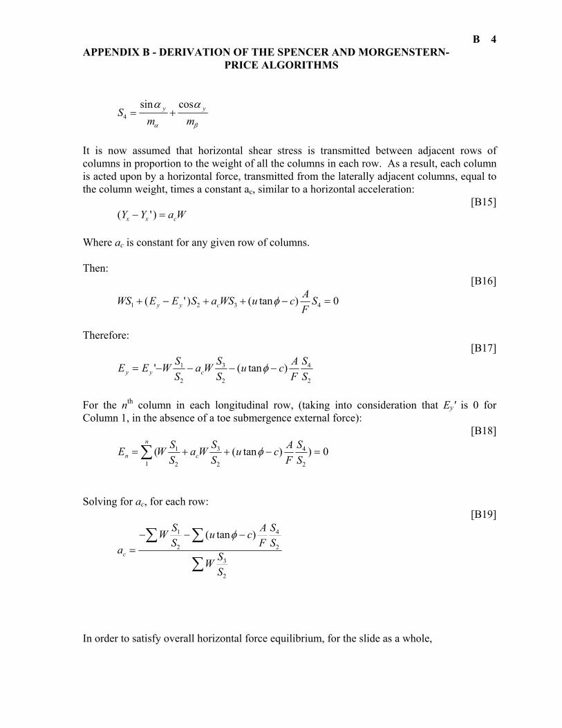
B APPENDIX B - DERIVATION OF THE SPENCER AND MORGENSTERN- PRICE ALGORITHMS
4
S
m my y
4 = +sin cosα α
α β It is now assumed that horizontal shear stress is transmitted between adjacent rows of columns in proportion to the weight of all the columns in each row. As a result, each column is acted upon by a horizontal force, transmitted from the laterally adjacent columns, equal to the column weight, times a constant ac, similar to a horizontal acceleration:
[B15] ( ' )Y Y a Wx x c− = Where ac is constant for any given row of columns. Then:
[B16]
WS E E S a WS u c A
FSy y c1 2 3 4 0+ − + + − =( ' ) ( tan )φ
Therefore:
[B17]
E E W S
Sa W S
Su c A
FSSy y c= − − − −' ( tan )1
2
3
2
4
2
φ
For the nth column in each longitudinal row, (taking into consideration that Ey' is 0 for Column 1, in the absence of a toe submergence external force):
[B18]
E W S
Sa W S
Su c A
FSSn
n
c= + + − =∑ ( ( tan ) )1
1
2
3
2
4
2
0φ
Solving for ac, for each row:
[B19]
aW S
Su c A
FSS
W SS
c =− − −∑∑
∑
1
2
4
2
3
2
( tan )φ
In order to satisfy overall horizontal force equilibrium, for the slide as a whole,

B APPENDIX B - DERIVATION OF THE SPENCER AND MORGENSTERN- PRICE ALGORITHMS
5
[B20] a W Fc n− =∑∑ 0
Where ΣFn is the sum of the horizontal forces and the sumation of acW is made over all the rows. The relationship between the vertical shear force, Xy and normal force, Ey, is given by an interslice force function, as defined by Morgenstern Price (1965):
λ)(xfEX yy = [B21] Where λ is a constant. The interslice force function is a constant for the Spencer's Method, or a half-sine function of distance from the crest and toe of the slide for the Morgenstern-Price method. The calculation now proceeds as follows: 1) Assume a value for λ 2) Calculate the value of ac for each column row from Eq. B19 3) Calculate the value of the normal forces Ey from Eq. B18 4) Calculate the value of the shear forces Xy from Eq. B21 5) Proceed with an iterative solution as used for Bishop's Simplified Method, adding the Xy
force resultants to the weights of the columns. 6) Change the value of λ iteratively, so as to satisfy Eq. B20
Reference: Morgenstern, N.R. and Price, V.E., 1965. The analysis of the stability of general slip surfaces. Geotechnique, 15:79-93.

________________________________
APPENDIX C
MATERIAL STRENGTH MODELS
________________________________

C APPENDIX C - MATERIAL STRENGTH MODELS
1
1) COULOMB ANISOTROPIC MODEL: This strength model is characterized by two cohesion values, cv and ch and two friction angles, φv and φh. The first value applies to the vertical orientation of the siding surface, the second to the horizontal. The actual cohesion and friction angle values in each column are calculated as elliptic functions of the dip of the sliding surface, γz. They are independent of the dip direction.
)21
(22 ]})(1[cos1{−
−−=h
vzv c
ccc γ
Eqn. [C1]
)21
(22 ]})(1[cos1{−
−−=h
vzv φ
φγφφ
Eqn. [C2] An example plot of cohesion variation with the dip angle is shown in Fig.C1. This model is useful for analysis of thinly interbedded horizontal sequences of weaker and stronger materials and weak rocks with horizontal fissility or closely spaced bedding joints. The use of an elliptic strength variation must be regarded as an approximation.
Fig. C1 Example of cohesion anisotropy
COHESION ON VERTICAL PLANES: cv = 500 kPa
COHESION ON HORIZONTAL PLANES: ch = 200 kPa
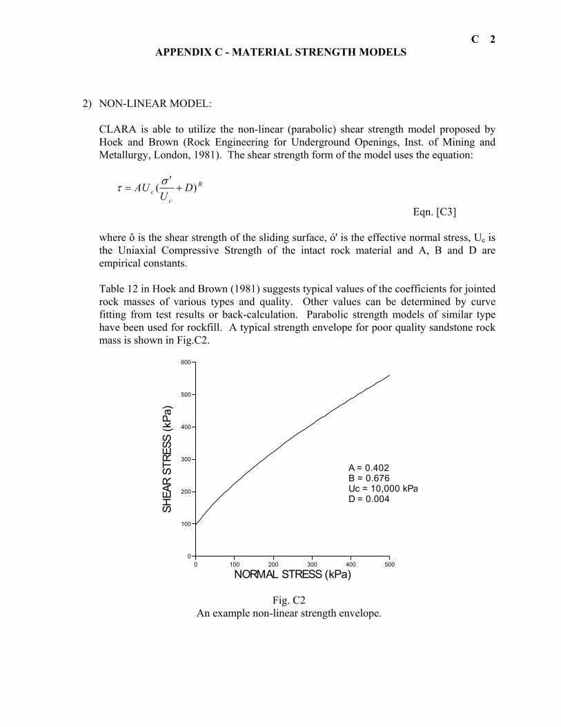
C APPENDIX C - MATERIAL STRENGTH MODELS
2
2) NON-LINEAR MODEL: CLARA is able to utilize the non-linear (parabolic) shear strength model proposed by Hoek and Brown (Rock Engineering for Underground Openings, Inst. of Mining and Metallurgy, London, 1981). The shear strength form of the model uses the equation:
B
cc D
UAU )( +
′=
στ
Eqn. [C3] where ô is the shear strength of the sliding surface, ó' is the effective normal stress, Uc is the Uniaxial Compressive Strength of the intact rock material and A, B and D are empirical constants. Table 12 in Hoek and Brown (1981) suggests typical values of the coefficients for jointed rock masses of various types and quality. Other values can be determined by curve fitting from test results or back-calculation. Parabolic strength models of similar type have been used for rockfill. A typical strength envelope for poor quality sandstone rock mass is shown in Fig.C2.
0 100 200 300 400 500
NORMAL STRESS (kPa)
0
100
200
300
400
500
600
SHEA
R ST
RESS
(kPa
)
A = 0.402B = 0.676Uc = 10,000 kPaD = 0.004
Fig. C2 An example non-linear strength envelope.

____________________________________________
APPENDIX D
LIST OF WARNINGS AND ERROR MESSAGES
____________________________________________

D APPENDIX D - LIST OF WARNINGS AND ERROR MESSAGES
1
CAN'T HAVE LESS THAN 1 ROW. The minimum number of rows is 1, which defines the problem as two-dimensional (see Par. B.2.3).
CAN'T HAVE MORE THAN 3000 COLUMNS.
The maximum number of columns is 3000. Note that using a large number of columns will affect the speed of the program.
CAN'T HAVE MORE THAN 3000 ROWS.
The maximum number of rows is 3000. Note that using a large number of rows will affect the speed of the program.
CAN'T HAVE MORE THAN 50 MATERIAL LAYERS. The maximum combined number of material layers is 50. CAN'T HAVE MORE THAN ONE SECTION IN 2D.
A two-dimensional problem can have only one input cross-section. The Control Parameters screen is used to change to three-dimensions.
CHOICE OF POINTS IS INCORRECT
The first scale point must be located to the left and below the second scale point (see Par. B.3.4).
COMBINED NUMBER OF MATERIALS AND DISCONTINUITIES MUST NOT EXCEED 50. The maximum combined number of material layers and discontinuities is 50. COMBINED NUMBER OF MATERIALS AND PIEZO SURFACES MUST NOT EXCEED 50. The maximum combined number of material layers and piezometric surfaces is 50. DISCONTINUITY # ... IS NOT ASSOCIATED WITH ANY PART OF THE SLIDING SURFACE.
This is just a reminder that the specified discontinuity is currently superfluous. Either delete it or associate it with a wedge surface plane (see Par. C.2.7).
ERR. HEAD OF SLIDE SUBMERGED.
CLARA-W has automatic provisions for toe submergence, (see Par. A.2.14). However, there is no provision for submergence of the head of the slide. Thus, CLARA-W cannot analyze a slide on the downstream face of an earth dam, the head of which extends into the reservoir on the upstream side.
ERR. LATERAL EQUILIBRIUM CANNOT BE ACHIEVED WITH THIS GEOMETRY. The balancing procedure requires that a part of the sliding surface has positive lateral slopes, while another has negative slopes. This is not the case, for example, where only one-half of a symmetrical problem is being solved.
D APPENDIX D - LIST OF WARNINGS AND ERROR MESSAGES
2
ERROR: MATERIAL # … : PROPERTIES INCORRECT. The specified material's properties are incorrect and must be changed in the Material Properties screen. The following problems cause this error to appear:
- The unit weight is missing. - The cohesion and/or the friction angle are negative for a coulomb isotropic
material. - The cohesion and the friction angle are both = 0 for a coulomb isotropic material. - The Cohesion and/or the friction angle are negative for an anisotropic coulomb
material. - The cohesion and the friction angle are both = 0 for an anisotropic coulomb
material. - The vertical cohesion and vertical friction angle are both = 0 for an anisotropic
coulomb material. - The uniaxial strength is negative for a non-linear material.
ERR. TENSION CRACK SPECIFIED TOO DEEP. The sliding surface is not sufficiently deep to accommodate the specified tension crack depth. ERR.: WRONG *.GRD FILE. USE 'EDIT STRATIGRAPHIC LAYER SURFACES' TO CORRECT. CLARA-W cannot read this grid file. Please modify it or load a different one.
ERR. - ZERO DRIVING FORCE. The specified sliding surface probably does not intersect the geometry. ERROR # … OCCURRED: .
An unknown error has occurred. It is advisable to restart the program to avoid any mishaps. FILE NOT FOUND. PLEASE TRY AGAIN.
The chosen file is not found in the chosen directory. Check spelling or check another directory.
GRID FILE USES DIFFERENT GRID PARAMETERS IN THE X (TRANSVERSE) DIRECTION. DO YOU WANT TO CONTINUE READING THIS FILE?.
The chosen grid file has a different Minimum X value, Maximum X value, and/or Number of Rows than those specified in the Control Parameters screen. If the file is read, then the current problem's Y dimensions will change to those of the grid file.
GRID FILE USES DIFFERENT GRID PARAMETERS IN THE Y (LONGITUDINAL) DIRECTION. DO YOU WANT TO CONTINUE READING THIS FILE?.
The chosen grid file has a different Minimum Y value, Maximum Y value, and/or Number of Columns than those specified in the Control Parameters screen for the current problem. If the file is read, then the current problem's Y dimensions will change to those of the grid file.
D APPENDIX D - LIST OF WARNINGS AND ERROR MESSAGES
3
INCORRECT *.GRD FILE.
The chosen grid file has less than two rows and/or columns, therefore it is not three-dimensional. Either modify the file or load a different one.
MIN. X MUST BE SMALLER THAN MAX. X. The mesh must extend from one X-coordinate to another which is larger (see Par. B.2.1). MIN. Y MUST BE SMALLER THAN MAX. Y. The mesh must extend from one Y-coordinate to another which is larger (see Par. B.2.1). MUST HAVE AT LEAST ONE MATERIAL LAYER. CLARA-W cannot define the problem geometry if there are no material layers. NO FILE LOADED.
Can't save because there is either no file loaded, or the file has no file name. Either start a new file, open a file, or use the Save As option under the File menu.
NO POINTS IN SECTION ... , LAYER ...
The specified layer in the specified section has no geometry points. Please complete the layer in the Edit Cross-sections screen.
ONLY … PIEZO SURFACES EXIST.
The Piezo Surface Number property of a material must be a positive integer equal to or less than the total number of piezometric surfaces in the problem.
ONLY 25 SECTIONS ALLOWED. The maximum number of input cross-sections allowed is 25. ONLY 50 POINTS ALLOWED.
The maximum permitted number of geometry input points for each layer is 50. Note that the first and last points must, respectively, lie before and beyond the defined start and end of the mesh.
PATH NOT FOUND. PLEASE TRY AGAIN. The chosen path is incorrect. Try another directory. PATH UNAVAILABLE.
No disk, drive is unavailable, or drive does not exist. Directory C:\ is automatically chosen instead.
SECTION … MUST BE ON OR BEYOND THE MAX. X POSITION.
To correctly define the mesh geometry, the last input cross-section must be on or beyond the Maximum X position.

D APPENDIX D - LIST OF WARNINGS AND ERROR MESSAGES
4
SECTION 1 MUST BE ON OR BEFORE THE MIN. X POSITION.
To correctly define the mesh geometry, the first input cross-section must be on or before the Minimum X position.
SECTIONS MUST INCREASE IN ORDER. The positions of all input cross-sections must increase in order from first to last. SELECTED DRIVE DOES NOT EXIST OR IS UNAVAILABLE.
The selected drive either does not exist on your machine or the drive door is open. Please select a disk drive available on your machine or insert a disk.
SURFACE DOES NOT INTERSECT GEOMETRY. Please re-define the sliding surface parameters.
THICKNESS CANNOT BE SPECIFIED FOR THIS SURFACE.
The ground layer is the highest layer, therefore it cannot be specified at a constant depth with respect to another surface.
THIS GRAPHIC HAS NOT BEEN CREATED YET.
The chosen graphic does not appear under the Window menu in the main screen, therefore has not been created yet or is not loaded. Please choose another graphic or create the appropriate one.
THIS SOLUTION IS NOT CONVERGING, TRY A DIFFERENT METHOD. The Spencers and Morgenstern-Price Methods sometimes fail to converge for certain problems. Try to change column spacing.
UBF/WT = … DO YOU WISH TO BALANCE LATERAL FORCES?. This geometry is unbalanced in the lateral direction. See Paragraph C.4.3 UNIDENTIFIED ERROR # … OCCURRED: … An unidentified error, as described, has occurred. It is advisable that you restart the program to avoid any mishaps. WAR. LESS THAN … ACTIVE COLUMNS FOR THIS SURFACE. The precision of the results may be impaired. Please read Par. C.4.7. WAR. M-ALPHA = … IN COLUMN … ROW … MAT'L …
The absolute value of the mα coefficient (Eqn. 2 of Hungr et al., 1989, see Appendix A) in a column is less than 0,001, indicating that the column may be carrying an unrealistically high portion of the total load. This is a common limitation with Bishop's method. The warning is associated with a beep sound. The value of the Factor of Safety is suspect. The sliding surface should be re-defined to make the angle in the vicinity of the subject column flatter.

D APPENDIX D - LIST OF WARNINGS AND ERROR MESSAGES
5
WAR. PIEZO SURFACE # ... IS NOT ASSOCIATED WITH ANY MATERIAL OR DISCONTINUITY.
This is just a reminder that the specified piezometric surface is currently superfluous. Either delete it or associate it with a material or discontinuity surface (see Par. C.2.7).
WAR. SLIDING MASS IS DISCONTINUOUS IN ROW … This message appears if, in any cross-section, the sliding surface daylights and then again dips under the ground surface. If an unnecessary part of the sliding surface projects downslope from the toe, you may truncate it by a discontinuity plane (see Par. C.2.7) with a Discontinuity Code 0, situated just above the toe and horizontal. Some 3D surfaces are legitimately discontinuous in certain cross-sections.
WAR. SLIDING SURFACE OUTSIDE PROBLEM BOUNDARY IN LATERAL DIRECTION. The sliding surface does not daylight in the lateral direction within the boundaries of the mesh. Please extend the mesh if necessary in the Control Parameters screen (see Par. B.2.3).
WAR. SLIDING SURFACE OUTSIDE PROBLEM BOUNDARY IN MOTION DIRECTION.
The sliding surface does not daylight in the motion direction within the boundaries of the mesh. Please extend the mesh if necessary in the Control Parameters screen (see Par.B.2.3).
WARNING, EXTERNAL FORCE ... IS OUTSIDE SLIDE BOUNDARIES.
The vertical components of any forces located outside the margins of the sliding surface will be ignored. Please read Par. A.2.15.
WARNING: LAYER ... IN SECTION ... DOES NOT EXTEND TO LEFT BOUNDARY.
Each layer in every section must start at a y-coordinate less than or equal to the start of the mesh y-coordinate, as specified in the Control Parameters screen (Par. B.2.3). Please complete the layer in the Edit Cross-sections screen (see Par. B.3.1).
WARNING: LAYER ... IN SECTION ... DOES NOT EXTEND TO RIGHT BOUNDARY.
Each layer in every section must finish at a y-coordinate greater than or equal to the end of the mesh y-coordinate, as specified in the Control Parameters screen (Par. B.2.3). Please complete the layer in the Edit Cross-sections screen.
WRONG FILE EXTENSION. MUST BE: … The saved file must have the specified extension, or enter the file name without any extension and the appropriate one will be automatically appended to the name.