Human-orthotic Integrated Biomechanical Model for Comfort Analysis … · Human-orthotic Integrated...
110
Human-orthotic Integrated Biomechanical Model for Comfort Analysis Evaluation Joana Evaristo Midões Baptista Dissertação para obtenção do Grau de Mestre em Engenharia Biomédica Júri Presidente: Professor Doutor Paulo Jorge Peixeiro de Freitas Orientador: Professor Doutor Miguel Pedro Tavares da Silva Professor Doutor Jorge Manuel Mateus Martins Vogais: Professor Doutor Paulo Rui Alves Fernandes Doutor Manuel Cassiano Neves Novembro 2011
Transcript of Human-orthotic Integrated Biomechanical Model for Comfort Analysis … · Human-orthotic Integrated...

Human-orthotic Integrated Biomechanical Model for Comfort Analysis Evaluation
Joana Evaristo Midões Baptista
Dissertação para obtenção do Grau de Mestre em Engenharia Biomédica
Júri
Presidente: Professor Doutor Paulo Jorge Peixeiro de Freitas Orientador: Professor Doutor Miguel Pedro Tavares da Silva Professor Doutor Jorge Manuel Mateus Martins Vogais: Professor Doutor Paulo Rui Alves Fernandes Doutor Manuel Cassiano Neves
Novembro 2011

II

I
Agradecimentos
Este espaço é dedicado àqueles que deram a sua contribuição para que esta tese fosse realizada.
A todos eles deixo aqui o meu agradecimento sincero.
Aos meus pais, Fátima e António, pela forma como me educaram e me incutiram os seus
melhores valores. Por serem os meus melhores amigos, pela força que me deram em todos os
momentos da minha vida e finalmente, pela confiança que depositaram em mim e nas minhas
escolhas desde sempre.
Ao Professor Miguel Tavares da Silva e ao Professor Jorge Manuel Mateus Martins pela orientação
do meu trabalho, pelas recomendações e incentivo que sempre me deram e pela boa-disposição com
que sempre me receberam. Um especial agradecimento ao Professor Miguel Tavares da Silva, pelas
muitas horas que generosamente me dedicou, transmitindo-me os seus conhecimentos com
paciência, lucidez e confiança e pelas palavras de ânimo que imprimiu sempre que necessário.
Aos meus colegas Marta Menezes, Sérgio Gonçalves e Carlos Vasconcelos, pelo apoio, ajuda e
disponibilidade que me dedicaram sempre que necessitei e pelo companheirismo e palavra de
incentivo nas alturas mais complicadas.
À Margarida Machado, pelos conhecimentos que me passou acerca do software e que me
ajudaram a progredir.
À comunidade OpenSim, e em especial ao Prof. Dr. Jeffrey Reinbolt e ao Prof. Dr. Ayman Habib,
pelo tempo que disponibilizaram a responder às minhas questões, pelos conhecimentos a nível do
software OpenSim e por algumas sugestões dadas, que contribuíram para o progresso do meu
trabalho, i. e., my sincere thanks to the OpenSim community, and especially to Prof. Dr. Jeffrey
Reinbolt. and to Prof. Dr. Ayman Habib, who provided the time to answer my questions, the
knowledge level of the OpenSim software and some suggestions, which contributed to the progress
of my work.
Aos meus colegas de trabalho por terem permitido que, numa última fase, pudesse ter o tempo e
disponibilidade necessários para a conclusão desta tese.
A todos os meus amigos e familiares, que de uma forma ou de outra me apoiaram durante este
tempo.
Por fim, queria dedicar um especial agradecimento ao Rodrigo Gomes, a pessoa que sempre
esteve ao meu lado. Pelas palavras de incentivo e confiança, pelo entusiasmo demonstrado pelo meu
trabalho, pelos momentos bons e outros menos bons, que fizeram parte deste percurso. Obrigada
por estares sempre lá.

II

III
Resumo
Nesta tese, foi desenvolvido um modelo de simulação e análise dinâmica, com o objectivo de
estudar a distribuição de forças de contact desenvolvidas na interface corpo humano/dispositivo
ortótico. O software utilizado para o desenvolvimento deste modelo foi o OpenSim, um software
para modelação, simulação, controlo e análise do sistema músculo-esquelético, que utiliza o Simbody
como interface de programação, e que é baseado baseado na dinâmica de corpos múltiplos.
Foram desenvolvidos dois modelos tridimensionais distintos: um modele de uma perna e pé
articulados entre si e um modelo de uma ortótese pé-tornozelo articulada. Estes dois modelos
tridimensionais foram definidos num só sistema multi-corpo, utilizando para tal os conceitos e
formulação disponibilizados pelo Simbody. O modelo de contacto Elastic Foundation foi aplicado
entre os dois protótipos, estabelecendo contacto entre eles. Foram prescritos alguns graus-de-
liberdade do sistema, utilizando dados experimentais cinemáticos e cinéticos adquiridos em
laboratório, de forma a garantir que o movimento resultante da simulação correspondesse a um ciclo
de marcha normal, não-patológica.
Finalmente, o valor da resultante das forças de contacto foi obtido, analisado e discutido e
algumas limitações do modelo de simulação desenvolvido são apresentadas assim como algumas
sugestões e direcções futuras para o posterior desenvolvimento e continuação deste trabalho.
Palavras-Chave: Modelo de simulação, análise dinâmica, distribuição de pressões, OpenSim,
Simbody, ortótese pé-tornozelo, Elastic Foundation, marcha não-patológica.

IV

V
Abstract
In this thesis, a dynamic analysis simulation model for analysis of contact forces distribution in the
human/orthosis interface is presented. The software used to develop this simulation model was
OpenSim, software for modeling, simulating, controlling, and analyzing the neuromusculoskeletal
system, which uses Simbody as the multibody dynamics engine to perform simulations.
Two distinct prototypes were developed: an articulated human leg and foot prototype and an
articulated ankle-foot orthosis prototype. These two prototypes were defined as a multibody system,
based on the multibody dynamic concepts and formulation of Simbody. The Elastic Foundation
contact model was used to establish contact between both prototypes. Some degrees of freedom of
the system were prescribed with kinematic and kinetic data, acquired in laboratory, ensuring that the
resulting movement of the simulation corresponds to a non-pathological gait cycle.
Finally, the resultant contact forces between both sub-systems were analyzed and discussed, and
some limitations of the simulation model were presented and future directions suggested, in order
continuing the development of the presented work.
Keywords: Simulation model, dynamic analysis, pressure distribution, OpenSim, Simbody, ankle-
foot orthosis, Elastic Foundation, non-pathological gait.

VI

VII
Contents
Resumo ................................................................................................................................................... III
Abstract ................................................................................................................................................... V
List of Figures .......................................................................................................................................... XI
List of Tables .......................................................................................................................................... XV
List of Symbols ..................................................................................................................................... XVII
Glossary .................................................................................................................................................. XI
Chapter I .................................................................................................................................................. 1
Introduction ............................................................................................................................................. 1
1.1 Motivation ..................................................................................................................................... 1
1.2 Literature Review .......................................................................................................................... 2
1.3 Objectives ...................................................................................................................................... 4
1.4 Main Contributions ....................................................................................................................... 5
1.5 Structure and Organization ........................................................................................................... 5
Chapter II ................................................................................................................................................. 7
Human Gait ............................................................................................................................................. 7
2.1 Coordinate Reference System for Gait Analyses ........................................................................... 8
2.2 Gait Cycle ....................................................................................................................................... 9
2.3 Gait Phases .................................................................................................................................. 11
2.3.1 Weight Acceptance .............................................................................................................. 11
2.3.2 Single Limb Support .............................................................................................................. 12
2.3.3 Limb Advancement ............................................................................................................... 13
2.4 Temporal Parameters .................................................................................................................. 14
2.5 Gait analysis ................................................................................................................................. 14
2.5.1 Kinematics ............................................................................................................................ 15
2.5.2 Kinetics ................................................................................................................................. 15
2.5.3 Electromyography ................................................................................................................ 16
Chapter III .............................................................................................................................................. 17
Orthoses ................................................................................................................................................ 17
3.1 Types of orthoses ........................................................................................................................ 17
3.1.1 Lower limb Orthoses ............................................................................................................ 17
3.2 Ankle Foot Orthoses .................................................................................................................... 21
3.2.1 Solid Ankle Foot Orthoses .................................................................................................... 21

VIII
3.2.2 Articulated Ankle Foot Orthoses .......................................................................................... 22
3.2.3 Leaf Spring Ankle Foot Orthosis ........................................................................................... 22
3.2.4 Ankle-Foot Orthoses Fabrication .......................................................................................... 23
3.3 Comfort and Tolerance Areas.................................................................................................. 24
Chapter IV ................................................................................................................................... 29
Simbody and Multibody Dynamics ........................................................................................................ 29
4.1 SimTK, Simbody and OpenSim .................................................................................................... 29
4.2 Fundamental Concepts and Multibody Mechanics Formulation ................................................ 30
4.2.1 Coordinate Frame ................................................................................................................. 30
4.2.2 Topology and Body Representation ..................................................................................... 31
4.2.3 Euler Angles .......................................................................................................................... 32
4.2.4 Generalized Coordinates ...................................................................................................... 34
4.2.5 Equations of Motion ............................................................................................................. 34
4.2.5.1 Kinematic Analysis ........................................................................................................ 34
4.2.5.2 Dynamic Analysis .......................................................................................................... 36
4.2.6 Bodies Mobilizers vs. Bodies Joints ...................................................................................... 38
4.2.7 Simbody Constraints ............................................................................................................. 40
4.2.8 Contact Models .................................................................................................................... 41
4.2.8.1 Hunt Crossley Contact Model ....................................................................................... 42
4.2.8.2 Elastic Foundation Model ............................................................................................. 44
Chapter V ............................................................................................................................................... 47
Simulation Model Definition ................................................................................................................. 47
5.1 3D acquisition of human anatomy .............................................................................................. 47
5.2 Geometric Modeling of the Leg and AFO Meshes ...................................................................... 47
5.3 Geometry Visualization Files ....................................................................................................... 50
5.4 Mass Properties ........................................................................................................................... 51
5.5 Defining Mobilizers between the Bodies .................................................................................... 53
5.6 Defining Contact Forces Between the Multibody System Bodies ............................................... 54
5.7 Prescribed Motion ....................................................................................................................... 56
5.7.1 Experimental Kinematic Data Acquisition ............................................................................ 56
5.7.2 Determining Joint Angles ..................................................................................................... 57
5.7.3 Trajectories ........................................................................................................................... 59
5.7.4 Ground Reaction Forces ....................................................................................................... 61
5.8 Running the Simulation ............................................................................................................... 65

IX
Chapter VI .............................................................................................................................................. 67
Results ................................................................................................................................................... 67
6.1 Computational Simulations ......................................................................................................... 67
Chapter VII ............................................................................................................................................. 79
Conclusions and Future Developments ................................................................................................. 79
7.1 Conclusions .................................................................................................................................. 79
7.2 Future Developments .................................................................................................................. 81
References ............................................................................................................................................. 83

X
XI
List of Figures
Figure 2.1- Marks described the walking process in eight organized phases and discussed the
relationship between prosthetic design and gait function (Marks 1907). .............................................. 7
Figure 2.2- Spatial reference system adopted. (Based on Winter, 1991) ............................................... 8
Figure 2. 3 - Divisions of the gait cycle. On the left it is represented the stance period. On the right it
is represented the swing period. In the sequence it is possible to see the onset of stance with IC, end
of stance/beginning of swing by roll off of the toes, and end of swing by floor contact again (Perry
1992)........................................................................................................................................................ 9
Figure 2. 4 - Step length is the interval between IC of each foot. Stride length continues until there is
a second contact by the same foot (Based on Perry J. 1992). .............................................................. 10
Figure 2. 5 - Divisions of the gait cycle (Based on Perry 1992). ............................................................ 11
Figure 2. 6 - Weight Acceptance period divided by two phases: Initial Contact and Loading Response
(Perry 1992). .......................................................................................................................................... 12
Figure 2. 7 - - Single Limb Support: Mid Stance, Terminal Stance and Pre Swing phases (Perry 1992).13
Figure 2. 8 - Limb Advancement Phases: Initial Swing, Mid Swing and Terminal Swing (Perry 1992). . 14
Figure 3.1 - Foot Orthosis types. Left: Custom made FO; Right: Off the Shelf FO. (Source:
www.orthotics-online.co) ..................................................................................................................... 18
Figure 3.2 - Knee Orthosis. a) Athletic KO; b) Non-Articulated KO; c) OTS KO. .................................... 19
Figure 3.3 - KAFO Types. a) Single/Double bar KAFO; b) Total contact KAFO; c) Weight Bearing KAFO.
............................................................................................................................................................... 19
Figure 3.4 - Hip Orthosis: a) Hip Abduction Orthosis; b) Hip Abduction Orthosis with KAFO extension;
c) S.W.A.S.H Orthosis............................................................................................................................. 20
Figure 3.5 - a) Example of a Hip Knee Ankle Foot Orthosis (HKAFO); b) Trunk Hip Knee Ankle Foot
Orthosis (THKAFO). ................................................................................................................................ 21
Figure 3.6 - Ankle Foot Orthosis Types a) Solid Ankle Foot Orthosis; b) Articulated AFO; c) Leaf Spring
AFO. ....................................................................................................................................................... 23
Figure 3. 7 - Areas and structures to be avoided in the lower limb: 1) Head of the fibula, 2)Patella, 3)
Knee condyles, 4) Tibial process, 5) Anckle malleolus, 6) Trochanter, 7) Achilles tendon, 8) Quadriceps
tendon, 9) Ischi-tibial tendons, 10) Groin, 11) Popliteal cavity, 12) Hip movement area 13) Knee
movement area, 14) Ankle movement area (Belda-Lois, Poveda et al., 2008). .................................... 25
Figure 3. 8 - Points for the analysis of PPT in the lower limb (Belda-Lois, Poveda et al., 2008). .......... 25
Figure 3. 9 – Hypothetical relationship between perceived sensation and contact area (Based on
(Goonetilleke, 1998)) ............................................................................................................................. 27
Figure 4. 1 - OpenSim organization and hierarchy structure: The base layer is the computational layer
provided by Simbody (blue); The next layer up is the modeling layer (green) that defines the model
and all its components. The analysis layer (orange) comprises a set of analyses, which fall into three
categories: modeler, solver, and reporter. The application layer (red) contains the OpenSim GUI, and
a set of utilities that exercise the OpenSim API directly. (Scott Delp, 2010). ........................................ 30
Figure 4.2 - Coordinate frame and axes convention in Simbody (Based on Sherman 2010). ............... 31
Figure 4.3 - Ground body representing the “0th” body in Simbody with his inertial reference frame
(left). Body В*i+, defined by his reference frame and origin OB[i]. ......................................................... 31

XII
Figure 4.4 - Rotations defining Euler Angles. The first rotation is about the X axis by an angle
followed by a rotation about the Y’ axis by an angle . The last rotation is about the Z’’ axis and is
rotated by an angle . (Based on (FERREIRA, 2008)). ....................................................................... 33
Figure 4.5 - Adding a body B to a multibody tree already containing parent body P (Based on Sherman
2010)...................................................................................................................................................... 40
Figure 4.6 - Constraint topology. This shows a single Constraint C with three constrained bodies Bk
and the outmost common ancestor body A (based on (Sherman 2010)). ............................................ 41
Figure 4.7 - Hunt and Crossley force Spheres, attached to different rigid bodies to simulate the
contact between the foot and the floor (Sherman, Seth et al., 2011). ................................................. 42
Figure 4.8 - Contact geometry for the Hertz/Hunt and Crossley model, for the two spheres contact
example (Sherman 2010). ..................................................................................................................... 43
Figure 4.9 - Elastic Foundation mesh-based forces for representing foot-floor contact in OpenSim
(Sherman, Seth et al., 2011). ................................................................................................................. 45
Figure 4.10 – Left and Middle: Two triangular mesh spheres (A and B), in contact. Right: Contact
between body A and body B with the Elastic Foundation Contact Model: Simbody determines each
triangles of A whose centroids are inside body B. S represents a point on body’s B surface, closest to
a centroid c located on body’s A polygon. A displacement x is determined as the distance from the
centroid to point S, for each polygon. ................................................................................................... 45
Figure 5. 1 - Left: First step on the 3D scanning, marking the reference points for the points cloud
creation; Middle: Reference points marked. Lower limb prepared to be scanned; Right: Points cloud
generated after the 3D scanning. This technique often introduces some points that are not part of
the scanned object, so the points cloud needs to be edited (Ana Luisa, 2010). .................................. 47
Figure 5. 2 - Creation of the lower limb geometry. Left: Points cloud obtained after the 3D scanning;
Middle: Transformation of the points cloud into a mesh, in SolidWorks; Right: Final mesh created in
SolidWorks, representing the human anatomy scanned. ..................................................................... 48
Figure 5. 3 - Creation of the Ankle-Foot Orthosis geometry based on the lower limb geometry. ....... 48
Figure 5. 4 - a) Articulated Ankle-Foot Orthosis with straps included that allow to adjust the AFO to
the patient’s leg (source: www.orthopedicmotion.com); b) Strap geometries, created in SolidWorks,
added to the former orthosis prototype. .............................................................................................. 49
Figure 5. 5 - Foot and Leg geometries obtained from cutting the lower limb prototype at the ankle
level. The images were taken from OpenSim software and illustrate the foot and leg rotation about
the ankle joint. ...................................................................................................................................... 49
Figure 5. 6 - The individual origin location for the six bodies defined in the multibody system. By
choice, the origin of all the bodies was placed at the same location, coincident with the ankle joint. 51
Figure 5. 7 - Definition of the different contact forces existing in the model: Only the contact forces
between the pairs of contact of interest to this work were defined. ................................................... 55
Figure 5. 8 - Marker set protocol: markers in anterior view (left) and lateral (right) view. .................. 56
Figure 5. 9 - Reference frames in QTM and OpenSim are not coincident. In order to have the
kinematic data consistent with the OpenSim reference frame it was necessary to make the
equivalent changes. ............................................................................................................................... 57
Figure 5. 10 - Definition of joint angles of lower limbs in sagittal plane (Winter 1991). ...................... 58
Figure 5. 11 - Joint angles obtained for the leg (top) and the ankle (bottom). ..................................... 59

XIII
Figure 5. 12 - Representation of body B and its Inertial frame trajectory vector, r. To translate body B
from a point P1 to a point P2 OpenSim expects to be given the body’s local frame trajectory vector, r’,
instead of vector r, as it would be expected. ........................................................................................ 60
Figure 5. 13 - Representation of arrangement in space of the eight IR cameras (red) used to acquire
the motion and the three force plates used to acquire the ground reaction forces (GRF) during the
stride period (white) (Based on (Gonçalves 2010). ............................................................................... 61
Figure 5. 14 - Conversion from action-oriented coordinate system (left) to reaction-oriented
coordinate system (right). ..................................................................................................................... 62
Figure 5. 15 - Conversion from reaction-oriented coordinate system (left) to OpenSim coordinate
system (right). ....................................................................................................................................... 63
Figure 5. 16 – Ground Reaction Forces in the antero-posterior axis. ................................................... 64
Figure 5. 17 – Ground Reaction Forces in the vertical y axis. ............................................................... 64
Figure 5. 18 – Ground Reaction Forces in the medial-lateral z axis. ..................................................... 65
Figure 5. 19 - COP values in the antero-posterior axis (left) and medial-lateral axis (right). Please note
that the vertical component of the COP is zero, at any instant. ........................................................... 65
Figure 6. 1 - Simulations kinematics obtained for the two distinct situations. Top: lower limb DOF
prescribed with experimental kinematic data and GRF applied to the plantar module of the orthosis.
Bottom: leg DOF prescribed and ankle joint left free for rotational movement. Orthosis joint
prescribed with the same kinematic as for ankle joint in the first situation. GRF also applied to the
orthosis’ plantar module. ...................................................................................................................... 67
Figure 6. 2 - Ground reaction forces represented as a single vector that combines, simultaneously,
vertical, sagittal and coronal forces. ..................................................................................................... 68
Figure 6. 3 – Critical points for analysis of PPT defined for the lower limb prototype. ........................ 69
Figure 6. 4 – Contact forces between the leg and the lateral module of the orthosis (normalized by
body mass). Top: results for the passive orthosis simulation; Bottom: results for the active orthosis
simulation. ............................................................................................................................................. 71
Figure 6. 5 - Contact forces between the leg and the lateral module of the orthosis (normalized by
body mass). Left: results for the passive orthosis simulation with no kinetics prescribed; Right: results
for the active orthosis simulation with no kinetics prescribed. ............................................................ 72
Figure 6. 6 - Contact forces between the foot and the plantar module of the orthosis (normalized by
body mass). Top: results for the passive orthosis simulation; Bottom: results for the active orthosis
simulation. ............................................................................................................................................. 73
Figure 6. 7 - Contact forces between the foot and the plantar module of the orthosis (normalized by
body mass). Left: results for the passive orthosis simulation with no kinetics prescribed; Right: results
for the active orthosis simulation with no kinetics prescribed. ............................................................ 74
Figure 6. 8 - Contact forces between the leg and the strap (normalized by body mass). Top: results for
the passive orthosis simulation; Bottom: results for the active orthosis simulation. .......................... 75
Figure 6. 9 - Contact forces between the foot and the strap (normalized by body mass). Top: results
for the passive orthosis simulation; Bottom: results for the active orthosis simulation. ..................... 77

XIV

XV
List of Tables
Table 2.1 - Sub-phases of the gait cycle as defined by major classification systems .............................. 8
Table 4.1 - Mobilizer types available in Simbody .................................................................................. 38
Table 5. 2 - Bodies and mobilizers used to connect these to their parent bodies. ............................... 53
Table 5. 1 - Anthropometric Data (Winter, 1991). ................................................................................ 53
Table 6. 1 - Point of pressure sensibility in the lower limb prototype. ................................................. 70
Table 6. 2 – Comparison of the contact forces maximum values with the MFT values established .... 78

XVI

XVII
List of Symbols
P - Pressure
F - Force
A - Area
θa – Ankle angle
θft – Foot angle
θh – Hip angle
θk – Knee angle
θlg – Leg angle
θth – Thigh angle
q – Vector of generalized coordinates
q – Vector of generalized velocities
q – Vector of generalized accelerations
– Kinematic constraints expressions
q – Jacobean matrix of in order to q
– Right-hand-side of the velocity equation
– Right-hand-side of the acceleration equation
*P - Virtual power produced by the external forces
f – Vector of all forces that produce virtual power (external and inertial forces)
g – Vector of generalized force *g – Vector of the generalized forces that contains the internal constraint forces
– Vector of Lagrange multipliers
M – Global mass matrix
fcontact – Contact force
fstiffness – Stiffness component of the contact force
fdissipation- Dissipation component of the contact force
ffriction - Friction component of the contact force
R -Relative radius of curvature E* - Composite elastic modulus
- Eccentricity factor K – Material stiffness of the Elastic Foundation model
*c - Effective dissipation coefficient
e - Coefficient of restitution

XVIII

XI
Glossary
AFOs - Ankle Foot Orthoses
PPT - Pain Pressure Thresholds
SRS - Spatial Reference System
CRS - Coordinate Reference System
IC - Initial Contact
GC - Gait Cycle
DLT - Direct Linear Transform
3D - Three-Dimensional
2D - Two-Dimensional
GRF - Ground Reaction Forces
EMG - Electromyography
FO - Foot Orthosis
AFO - Ankle Foot Orthoses
KO - Knee Orthosis
KAFO - Knee Ankle Foot Orthosis
HO - Hip Orthosis
HKAFO - Hip Knee Ankle Foot Orthoses
THKAFO - Trunk Hip Knee Ankle Foot Orthoses
OTS - Off the Shelf
SST - Spatial Summation Theory
CAD - Computer Aided-Design
MPT - Maximum Pressure Tolerance
MFT – Maximum Force Tolerance
PPT – Pain Pressure Threshold
API - Application Programming Interface
ODE - Ordinary Differential Equations
DAES - Differential Algebraic Equations

XII

1
Chapter I
Introduction
1.1 Motivation
Ankle foot orthoses (AFOs) are orthotic devices often prescribed to support, re-align or
redistribute pressure across a musculoskeletal system. The use of these devices can lead to a
reduction in symptoms, improvement in function, and may result in an increase of the patient’s
quality of life and walking performance (Braddom and Buschbacher, 2000).
AFOs and orthotic devices in general, have undergone a huge evolution over the past 50 years
with regard to materials used in its manufacturing. From stainless steel (Felts, 2005) to thermoplastic
materials (Meyer Jr, 1974), changes had lead to an advancement and improvement on AFOs
characteristics. Therefore, these advances reflected in increased performance, efficiency and comfort
for patients.
The techniques used in AFOs manufacturing have also been subject of intense study, since current
techniques are time-consuming and do not rely on systematic engineering. Instead, techniques used
nowadays require experienced craft-persons that make their decisions based on experience and trial-
and-error methods (Silva P., 2008; Pallari, Dalgarno et al., 2010). The development of different
methods for manufacturing orthotic devices, customized for specific patients, could lead to AFOs
topology optimization and enhancing of patients performance while using these devices.
Although much has been done in research of new materials and manufacturing techniques,
almost no research has been done regarding the pressure distribution in the patient/orthosis
interface.
Motion control and comfort are the primary objectives in orthotics and one of the principal
parameters to evaluate comfort is the pressure distribution in the human body/orthosis surface.
However, the ideal pressure distribution between the human body and any given surface area is not
well defined (Goonetilleke, 1998).
Comfort is an important variable and could have many definitions. For example, it could be the
lack of discomfort or a feeling of well-being (Zhang, Helander et al., 1996), which are two different
types of comfort measure. It is, in fact, much easier to define discomfort. Discomfort or pain
originates when special nerve endings, called nociceptors, detect an unpleasant stimulus and some
believe that pain signals must reach a threshold before they are relayed (Goonetilleke, 1998).
Most studies on the issue of comfort are made in the field of Foot Orthoses or Shoe Inserts,
especially regarding their prescription and benefits in sport activities (Nigg, NURSE et al., 1999;
Mündermann, Stefanyshyn et al., 2001; Mündermann, Nigg et al., 2002; Mündermann, Nigg et al.,
2003; Davis, Zifchock et al., 2008). Nothing has been done to date in order to study the distribution
of pressures in AFOs and consequently, the interface forces developed in the patient/orthotic device
interface. Furthermore, no study has compared these pressures/forces with levels of pain pressure
thresholds (PPT)/maximum force tolerance (MFT), that may be on the basis of the discomfort felt by
people who use these orthotic devices. The information and results of such studies can lead to a
“revolution” in AFOs topology, and can be applied clinically in old and new AFOs projects/prototypes,
improving and analyzing their efficiency.

2
1.2 Literature Review
The concept of assistive technology, namely orthotic devices, exists for many centuries.
Historically, orthotic devices have been used for the treatment of musculoskeletal injuries or
dysfunctions and have provided support, protection, immobilization and correction.
In the 1950s new materials and fabrication techniques started to be used, which changed and
improved orthotic devices. At that time, stainless steel was the most used material by orthotists
because of its strength, adaptability and durability (Poitout, 2004; Felts, 2005).
The aluminum spring brace was introduced in the late 60s (Magora, Robin et al., 1968; Robin and
Magora, 1969). Although with less strength, aluminum was easier to work and cosmetically more
attractive then stainless steel.
Due to the demand of orthotic devices with a more attractive appearance, in the 1970s new
techniques like plastic coating were developed, allowing the improvement of the orthoses
appearance by applying a tinted rubber-based plastic film (Meyer Jr, 1974). Also in this decade, the
use of thermoplastic materials was adopted in the rehabilitation field (Doxey, 1985). Polypropylene
and polyethylene were the most popular ones due to their high fatigue resistance, strength, light
weight and good molding characteristics.
In the early 1980s new varieties of thermoplastic ankle foot orthoses (AFOs) were designed and
prescribed and gait patterns were studied with these new orthotic devices (Meyer Jr, 1974). Leone
predicted the force on AFOs using a simple structural model analysis (Leone, 1987) and the stress
distribution in a polypropylene ankle foot orthosis (AFO) was determined with a two-dimensional
(2D) finite-element model (Reddy NP, 1985).
In the 1990s decade, three-dimensional (3D) finite-element models were developed in order to
study the stress distribution in polypropylene AFOs (T. Chu, 1990; T. Chu, 1995), determining failure
mechanisms and localization of weak points. Researches were also carried out to study the effect of
patient’s body geometry on the design parameters (T. Chu, 1998; Chu, 2000), concluding that
variations of stress had their individual characteristics, varying according to different motions, foot
geometry, and types of AFOs. Chu et al. tried to develop a new design and manufacture technique
for polypropylene AFOs, integrating computer-aided design and manufacturing software, in order to
reduce manufacturing steps and costs (A. Candan, 2000).
In addition to studying design, many researchers started to investigate the effects of different
types of AFOs on patients’ walking patterns. Mueller et al. studied the effect of a Dynamic AFO
(DAFO) on the foot-loading pattern in hemiplegic patients, concluding about the positive and
immediate effect of these particular type of AFOs (Mueller, Cornwall et al., 1992). Dieli et al. also
studied the effect of DAFOs on Hemiplegic adults finding good results in the application of these
orthotic devices as an alternative treatment to conventional thermoplastic orthoses (Dieli, Ayyappa
et al., 1997). Abel et al. studied gait assessment of fixed ankle-foot orthoses in children with Spastic
Diplegia (Abel, Juhl et al., 1998), while Thomson et al. studied the effects of ankle-foot orthoses on
the ankle and knee in persons with Myelomeningocele (Thomson, Ounpuu et al., 1999). The
influence of AFOs on gait and energy expenditure in patients with Spina-Bifida and the long-term
effects of ankle-foot orthosis on patients with unilateral Foot Drop were also explored (Duffy,
Graham et al., 2000; Geboers, Drost et al., 2002).
Ahead, the effectiveness of custom foot orthoses in different types of foot pain were evaluated by
Hawke (Hawke, Burns et al., 2008). This study revealed that the evidences on which to base clinical

3
decisions for prescription of custom foot orthoses were limited, concerning the treatment of foot
pain.
A few years ago the feasibility of using new technique approaches, in the manufacture of
customized orthoses and prosthetics, started to be investigated. The studies were performed both in
orthotic and prosthetic fields since the manufacturing of both devices was, and still is, very similar.
These new techniques explored the use of 3D human scanning, orthotic or prosthesis design with
CAD and automated production.
Faustini developed compliant structures for prosthesis, based on these new techniques, and
analyzed them using the finite element method. He found that contact pressures between the
residual limb and the produced prosthesis could be significantly reduced with an integrated
compliant surface (Faustini, 2004). Further, Faustini et al. investigate the feasibility of custom made
AFOs and on how to adjust their stiffness, concluding that these new methods approach were well
suited for AFO production (Faustini, Neptune et al., 2008).
Pallari et al. explored additive manufacturing techniques such as selective laser sintering (SLS), a
technique that uses a high power laser to fuse small particles of plastic, metal and others (Langer,
Wilkening et al., 2000), into a mass with the desired 3D shape. They stated that the clinical
performance of foot orthoses (FOs) fabricated using SLS was comparable to those produced using
traditional methods. They compared their results to the processes used nowadays, and in
comparison with these artisan manufacturing methods, they enhanced the potential of this approach
in the improvement of quality, consistency and patient care (Pallari, Dalgarno et al., 2010; Pallari,
Dalgarno et al., 2010). Pallari et al. concluded that SLS process was ideally suited in this application,
suggesting that future studies should focus on modifying the AFOs design, in order to optimize and
improve patient performance, developing a manufacturing framework for fabricating customized
AFOs to specific patients. Pallari et al. also investigate the effect of different materials and different
design characteristics on functional parameters of AFOs. Topology optimization was used to find the
optimal material distribution for the AFO. Examples of where improvements to current systems could
be made, using tailored software solutions, were showed (Pallari, Dalgarno et al., 2010).
In general, comfort is an important and relevant feature of AFOs. Evaluations of these orthotic
devices concerning comfort will reflect personal perceptions and differences due to biomechanical
variables. Defining the relationship between comfort and biomechanical variables such as material
modifications, surface area and different modes of locomotion is crucial in the optimization of AFOs
topology. Most of the studies done so far concerning comfort are made relative to Footwear, and
until date no study about comfort in AFOs was found.
Mündermann tried to determine the relationship between comfort and changes in lower limb
kinematic, kinetic variables and muscle activity, in response to foot orthoses (Mündermann, Nigg et
al., 2003). He claimed that footwear modifications including material and shape showed to affect
these functional variables during locomotion. Based on his research, he stated that footwear
modifications can be perceived by subjects and that these modifications affect their subjective
comfort in locomotor tasks such as running and walking. He also stated that these effects may be
different between walking and running. However, he concluded that no evidences had been
provided as to whether comfort was in fact related to lower extremity kinematics, kinetics, and
muscle activity during locomotion and suggested that the factors that are important for orthotic
comfort are not well understood.
Finestone et al. studied the acceptance rates and comfort scores of soft custom, soft
prefabricated, semi-rigid biomechanical, and semi-rigid prefabricated orthoses and their effect on

4
the incidence of stress fractures, ankle sprains, and foot problems (Finestone, Novack et al., 2004).
They proved that soft-custom and soft-prefabricated orthoses had significantly higher comfort scores
than the semi-rigid biomechanical and prefabricated orthoses.
Silva et al. developed a multibody model in 2D consisting of two sub-models: an AFO sub-model
and a human sub-model attached by means of non-linear force elements. Contact was defined
between both sub-systems using a non-linear continuous contact/impact force model that accounts
for the stiffness and damping characteristics of the surfaces in contact. Their main goal was to
optimize the force distribution at the lower limb/orthosis interface for comfort design. Preliminary
results showed that interface forces and corresponding contact areas can be carried out and used in
the design of orthotic devices (Silva P., 2008).
The latest literature indicates that the assumption of using different methods for manufacturing
orthotic devices is feasible. Some studies tried to show how the shape of the orthotic devices can be
altered to save weight, improve functional properties, be more suitable and patient customized.
Orthoses can be highly customized, through the incorporation of gait and surface pressure
measurement analysis into the design process. However, this is not done in current clinical practice.
This is mostly because of time, cost and manufacturing constraints since the orthotic and prosthetic
industry does not have a tradition of engineering and expert design.
Orthoses are widely prescribed both to treat existing pathological conditions and to prevent
overuse injuries but little is known about the effect of their material composition and fabrication
technique on patients’ comfort. The inclusion of parameters such as comfort, in the orthotic devices
design, and the development of engineering software to design and analyze orthoses, may improve
orthotic product design creating completely new kinds of products. This will change the industry
currently restricted by old and inefficient manufacturing methods.
1.3 Objectives
The main objective of this work is to calculate the contact forces distribution at the interface of an
orthotic device prototype with a human leg and foot, both in contact, through a forward dynamic
simulation. The simulation will be performed for a non-pathological gait cycle movement.
To reach that objective, it is necessary to model two 3D prototypes: a detailed 3D prototype of a
hinged AFO, in this specific case; a detailed 3D prototype of a human leg and foot, articulated. After
developing these two prototypes, a multibody system must be defined and its topological structure
settled. In addition, it is also essential to define a contact model between the two prototypes, to
obtain the interface forces.
Once defined the multibody system, in order to simulate the non-pathological gait cycle it is
necessary to prescribe some degrees of freedom of the multibody system, and for that experimental
kinematic and kinetic data will be used.
Finally, the interface forces resulting from contact between the two sub-systems is analyzed and
the peaks of high interface forces are evaluated ,concerning the MFT and tolerance areas (Belda-Lois,
Poveda et al., 2008), to discuss matters of comfort.
This work was developed under the scope of the FCT project DACHOR-Multibody Dynamics and
Control of Active Hybrid Orthoses (MIT-Pt/BS-HHMS/0042/2008).

5
1.4 Main Contributions
This thesis aims to be a step in the study of interface forces distribution in the area of Ankle-Foot
Orthoses. Also, this work is intended to relate these forces with MFT values, relate these with
comfort issues and analyze possible changes that could be made concerning the topology of these
orthotic devices. Therefore, this work is the first effort towards the advance of AFOs topology
optimization.
To date, this is the first detailed tridimensional model of an articulated AFO and articulated
human leg and foot system whose definition is based on the dynamic multibody formulation,
completely customizable and capable of adapting to different geometries of human body or other
orthoses.
The adaptability of this model turns it into a potential tool of analysis of actual, and yet to come,
orthoses prototypes/projects. Also, this model can be adapted to study the orthoses efficiency not
also in different non-pathological human gaits, but also in pathological gaits of different types, since
the experimental data used to simulate movement was acquired in a biomechanical laboratory.
In addition, this is the first known dynamic analysis attempting to study this subject in this area or
similar areas, like Foot Orthoses or Lower Limb Orthoses, since most of the studies are made using
static analysis.
The work in this thesis is a step forward in biomechanical simulation, trying to merge several
areas together in order to take full advantage of each individual area. Areas like Multibody Dynamics,
3D scanning, 3D modeling and meshing, Kinematic and kinetic acquisition and contact modeling are
used in this work in order to create a simulation model that in the future might be developed and
used as a powerful analysis tool.
1.5 Structure and Organization
Chapter I – The first chapter is an introduction to work in this thesis. A literature review and the main
motivations and objectives of this work are presented, as well as the major contributions that arise
after its development.
Chapter II – In this chapter, a review in the study of human gait is presented. Some terminology and
concepts needed to describe gait analysis are referred and the gait phases of a gait cycle are
explained in detail. A brief review on the concepts behind kinematic, kinetic and electromyography
analysis is made.
Chapter III – The third chapter presents a brief review to the lower limb orthoses with special
attention to the AFOs, since they represent the type of orthosis used in this thesis. The current and
different techniques of manufacture of these devices are described and listed the most used
materials. Finally, the Spatial Summation Theory is presented and described, which relates the
pressure values with the contact area and possible comfort / discomfort sensations. The pressure
tolerance areas for the lower limb are also described.
Chapter IV – Simbody, OpenSim’s multibody dynamics engine to perform simulations, is presented. A
brief introduction and overview is made, followed by a detailed description on the mechanical
concepts and multibody dynamics formulation used by this software. The equations of motion for
kinematic and dynamic analyses are described. Finally, the contact models available by this
biomechanical simulation tool are briefly described.

6
Chapter V –In this chapter, the methodologies used to create the 3D multibody system and
simulation model are presented. The process of acquisition of human morphology for the
construction of the lower limb prototype and posterior development of the articulated AFO
prototype is explained in detail. The 3D modeling and meshing techniques are presented as well as
the multibody system definition and topology structure adopted. The contact model implementation
is explained and the contact forces parameters are defined. Finally, the methods and equipment
used in the acquisition of kinematic and kinetic experimental data are presented as well as the
calculations necessary to perform, in order to prescribe the non-pathological movement to the
system.
Chapter VI – The results of prescribing kinematic and kinetic data to the simulation model are
showed. The analysis and discussion of the results is made concerning several simulations performed
for two distinct situations: Passive ankle foot orthosis and Active ankle foot orthosis.
Chapter VII – Most relevant conclusions of the work are discussed and presented and some
considerations for future developments and related works are also mentioned and described. Future
applications for the simulation model developed in this work are suggested.

7
Chapter II
Human Gait
Normal human gait can be defined as a method of locomotion involving the use of the two legs,
alternately to provide both support and locomotion (Whittle, 2001). In the last decades, gait science
has been suffered an enormous development, producing a series of terms and concepts related to
observational gait analysis (Ayyappa, 1997).
In 1907, A.A. Marks, an American prosthetic, offered a precise qualitative description of normal
human locomotion when he illustrated and analyzed the walking process in eight organized phases
and discussed the implications of prosthetic design on the function of amputee gait (see Figure 2.1)
(Marks, 1907).
Figure 2.1- Marks described the walking process in eight organized phases and discussed the relationship
between prosthetic design and gait function (Marks 1907).
Over the years, a series of contributions have increased the understanding of gait science and
terminology. Among others, Saunders et al. studied the major determinants in normal and
pathological gait (Saunders, Inman et al., 1953); Sutherland et al., studied gait disorders and gait
kinematics and kinetics (Sutherland, Schottstaedt et al., 1969; Sutherland, Olshen et al., 1980;
Sutherland, 1984; Sutherland, Kaufman et al., 1994); The work of Jacquelin Perry resulted in
descriptive terms for the phases and functional tasks of gait (Hospital, 1977; Perry, 1992).
There have been various classifications explaining the phases, sub-phases and events occurring
during a complete gait cycle. The most commonly used classification systems were those developed
by Olney, Perry, Whittle, Sutherland and Vaughan (Perry, 1992; Sutherland, Kaufman et al., 1994;
Vaughan CL, 1999; Whittle, 2001; Olney, 2005).
Although there are several distinct classifications, all the classifications agree on the division of
gait cycle into two phases: stance and swing phases. The phases are further categorized to sub-
phases, which are periods in the gait cycle spanning two points in the gait cycle, and events: specific
points in the gait cycle which are considered to be relevant. The sub-phases described by various
authors are compared in Table 2.1.

8
It can be seen from Table 1 that Whittle has adopted Perry classification of sub-phases. Also
Vaughan suggested that the gait of some pathological individuals cannot be described using his
terminology (Vaughan CL, 1999).
Table 2.1 - Sub-phases of the gait cycle as defined by major classification systems
Perry (1992) Sutherland (1994) Vaughan (1999) Whittle (2001) Olney (2005)
Initial contact
Initial Double Support
Initial contact Initial contact
Heel Strike Loading response
Foot Flat Loading
response
MidStance Single Limb Support MidStance MidStance MidStance
Terminal Stance Second Double Support
Heel Off Terminal Stance Push Off
Pre-Swing Toe Off Pre-Swing
Initial Swing Initial Swing Acceleration Initial Swing Acceleration
Mid-Swing Mid-Swing Mid-Swing Mid-Swing Mid-Swing
Terminal Swing Terminal Swing Deceleration Terminal Swing Deceleration
Although these classifications could be perfectly applied to describe the gait of non-pathological
subjects, the nomenclature presented by Perry proved to be the most generally applicable to
describe any type of gait (Vaughan CL, 1999).
2.1 Coordinate Reference System for Gait Analyses
A spatial reference system (SRS) or coordinate reference system (CRS) is a coordinate-based local
or global system used to locate geographical entities. The spatial reference system usually changes
from author to author, but all follow the right hand rule to define the three orthogonal vectors
(Winter, 1991). Vaughan uses X to define the direction of progression, Y lateral direction and Z to
vertical direction and Winter uses the X axis to define the direction of progression, Y vertical
direction and Z lateral direction (Winter, 1991; Vaughan CL, 1999). In this thesis the reference system
used is the same as Winter (see Figure 2.2).
Figure 2.2- Spatial reference system adopted. (Based on Winter, 1991)

9
2.2 Gait Cycle
Walking uses a repetitious sequence of limb motion to move the body forward while
simultaneously maintaining stance stability. Because each sequence involves a series of interactions
between two multi-segmented lower limbs and the total body mass, identification of the numerous
events that occur necessitates viewing gait from several different aspects (Perry, 1992).
According to Perry, the gait cycle can be approached from three different ways. The simplest way
is to divide the gait cycle in phases according to the variations in reciprocal floor contact of the two
feet, the second way divides the gait cycle by the time and distance qualities of the stride and the
third way (the most common) is to identify the most significant events within the gait cycle,
designating these intervals as the functional phases of gait.
The gait cycle is the period of time between any two identical events in the walking cycle. One gait
cycle of a limb normally extends from the point when the heel of the reference limb touches the
ground, to the same happening again (Olney, 2005). Generally, in gait studies, the gait descriptions
considers only a single cycle, assuming that all the cycles are equal. However, this fact is not strictly
true, but it is a reasonable approximation (Vaughan CL, 1999). Hence, any event could be selected as
the onset of the gait cycle. Normal persons initiate floor contact with their heel (i.e., heel strike)
although, not all patients have this capability. Perry named this event with the generic term Initial
Contact (IC), and this term will be used as the offset of the gait cycle.
According to all classifications reviewed each gait cycle is divided into two periods, stance and
swing (see Figure 2.3). The stance phase forms 60% of the gait cycle and occurs when the reference
limb is contact with the ground, beginning with initial contact. Swing phase occurs when the
reference limb is not in contact with the ground (swinging), which forms the remaining 40% of the
gait cycle, and applies to the time the foot is in the air.
Figure 2. 3 - Divisions of the gait cycle. On the left it is represented the stance period. On the right it is represented the swing period. In the sequence it is possible to see the onset of stance with IC, end of stance/beginning of swing by roll off of the toes, and end of swing by floor contact again (Perry 1992).
Stance period can be divided in three intervals depending on the contact of the feet with the
floor. The first interval is the Initial Double Stance that begins the gait cycle, when both feet are on
the floor (after IC).After that, the Single limb Support begins when the opposite foot is lifted for
swing. The stance period ends with the Terminal Double Stance, when the other foot contacts the
floor and goes until the reference foot is lifted for swing.
A gait cycle can also be identified by the term stride which is the equivalent of a gait cycle (see
Figure 2.4). The duration of a stride is the interval between two sequential initial floor contacts by
the same limb. The interval between IC of each foot is a step (i.e., left and then right).

10
Figure 2. 4 - Step length is the interval between IC of each foot. Stride length continues until there is a second
contact by the same foot (Based on Perry J. 1992).
Despite this approaches, classify a gait by phases allows to a better interpretation of the different
motions that occur during a gait cycle. According to Perry, there are three basic tasks that should be
accomplished by the limb: Weight Acceptance, Single Limb Support and Limb Advancement. Within
these tasks, eight distinct phases were defined: Initial Contact, Loading Response, Mid-Stance,
Terminal Stance, Pre-Swing, Initial Swing, Mid-Swing and Terminal Swing.
Weight Acceptance begins the stance period and uses the first two gait phases: Initial Contact and
Loading Response. Then Single Limb Support continues stance with Mid-Stance and Terminal-Stance
phases. Finally, Limb Advancement begins in the final phase of stance with the Pre-Swing phase and
continues through the three phases of swing: Initial Swing, Mid-Swing and Terminal Swing.

11
.3 Gait Phases
As mentioned above, there are three main tasks that should be accomplished by the limb and
within those tasks Perry divided the gait cycle in eight phases. Figure 2.5 illustrates this division, for a
better understanding.
2.3.1 Weight Acceptance
The Weight Acceptance is the most demanding task, requiring the abrupt transfer of body weight
into the limb that has just finished swinging forward. It begins with the shock absorption then, the
limb stability and the preservation of progression. These three functional patterns are divided in two
phases: Initial Contact and Loading Response (see Figure 2.6).
Initial Contact (Phase 1)
This phase occurs in the moment the foot touches the floor, representing 2% of the gait cycle
(GC). During the IC the floor contact is made with the heel, the hip is flexed at approximately 300, the
knee totally extended and the ankle is dorsiflexed to neutral.
Loading Response (Phase 2)
Loading Response represents about 10% of the GC and begins with the initial floor contact by the
foot, continuing until the other foot is lifted for swing. This phase is characterized by the absorption
of the shock from the impact of foot with ground and by the weight acceptance. At this stage, the
body weight is transferred onto the forward limb (reference limb) and, using the heel as a rocker, the
knee is flexed for shock absorption. The opposite limb is in its Pre-Swing phase.
Figure 2. 5 - Divisions of the gait cycle (Based on Perry 1992).

12
Figure 2. 6 - Weight Acceptance period divided by two phases: Initial Contact and Loading Response (Perry
1992).
2.3.2 Single Limb Support
This period begins when the other foot is lifted for swing, continuing until that same foot contacts
the floor, being the reference limb totally responsible for supporting the body weight in sagittal and
coronal planes. There are two phases involved in this period: Mid Stance and Terminal Stance.
Mid Stance (Phase 3)
Mid Stance represents the first half of the Single Limb Support period when the limb advances
over the stationary foot by ankle dorsiflexion while the knee and hip extend (see Figure 2.7). The
opposite Iimb is advancing in its Mid-Swing phase with the restrained ankle dorsiflexion, knee
extension and hip stabilization in coronal plane. This phase corresponds to the interval [10%, 30%] of
the GC.
Terminal Stance (Phase 4)
The second half of the Single Limb Support is the Terminal Stance (see Figure 2.7), representing
30%-50% of the GC. In this phase, the heel rises, the knee increases its extension and then just begins
to flex slightly and continues until the other foot strikes the ground.
Pre Swing (Phase 5)
Pre-Swing is the final phase of Stance and the initial phase of Swing, beginning with IC of the
opposite limb and ending with ipsilateral toe-off (see Figure 2.7). It represents 50%-60% of the gait
cycle. In this phase the body weight transfer unloads the reference limb while this prepares for the
Swing period. The reference limb responds with increased ankle plantar flexion, greater knee flexion
and loss of hip extension. The opposite limb is in Loading Response.

13
Figure 2. 7 - - Single Limb Support: Mid Stance, Terminal Stance and Pre Swing phases (Perry 1992).
2.3.3 Limb Advancement
Initial Swing (Phase 6)
The Initial Swing phase begins when the foot is lifted from the floor and ends when the swinging
foot is opposite the stance foot (see Figure 2.8). This phase is characterized by an increased knee
flexion (about 600), preventing the dragging of the foot in the ground and also by the hip flexion, in
order to advance the limb. The other limb is in early Mid-Stance. This phase occurs approximately at
60%-73% of the GC.
Medial Swing (Phase 7)
During the Medial-Swing phase the swinging limb is opposite the stance limb (see Figure 2.8) and
it will go until the swinging limb is forward and the hip and knee flexion postures are equal. This
phase occurs in the 73%-87% of the GC interval and it is marked by a knee flexion decrease (until
300).
Terminal Swing (Phase 8)
In the Terminal Swing phase (87%-100% of the GC) the reference limb advancement is completed
by the knee extension. The hip maintains its earlier flexion and the ankle remains dorsiflexed to
neutral. The phase ends when the foot contacts the floor (Figure 2.8), preparing the Stance phase
again, while the opposite limb is in Terminal Stance.

14
Figure 2. 8 - Limb Advancement Phases: Initial Swing, Mid Swing and Terminal Swing (Perry 1992).
2.4 Temporal Parameters
Gait parameters related to time are referred to as temporal parameters. Stride length, cadence
and velocity are three important interrelated temporal parameters. Commonly misused, the terms
step length and stride length are not synonymous. Like explained above, the duration of a stride is
the interval between two sequential initial floor contacts by the same limb and a step is defined by
the interval between IC of each foot (see Figure 2.4).
Cadence refers to the number of steps taken per unit of time and is the rate at which a person
walks expressed in steps per minute. Natural or free cadence describes a self-selected walking
rhythm (Ayyappa, 1997).
Velocity combines stride length and cadence and is the resultant rate of forward progression
along the direction of progression, measured over one or more strides, and is expressed in meters
per second (Ayyappa, 1997).
2.5 Gait analysis
There are a wide variety of different types of human walking gait, for example that on an average
human being, which is generally described as normal gait, and that of a physically impaired human
being, which is generally referred to as abnormal gait. Physically impaired human beings include
persons that suffer from cerebral palsy, and people who had suffer strokes, head injuries or spinal
injuries (O'Malley and de Paor, 1993), just to mention some of the most usual gait pathologies.
Gait analysis is the study of walking gait and is used as a clinical tool by medical doctors to decide
on the treatment of abnormal gait.
There are three distinct categories of gait analysis: kinematics, i.e. the study of movement both
temporal and spatial (Winter 1991); kinetics of the foot-floor and joint forces; and the study of the
muscle activity, i.e., electromyography.

15
2.5.1 Kinematics
Measurements of individual joint angular rotations, as well as translations of segments and of
whole body mass, allow the comparisons with normal that are necessary to distinguish pathological
from normal gait (Sutherland, 2002).
Kinematic analysis observes and describes the motion of objects without consideration of the
causes leading to the motion (Robertson, 1997), focusing on joint motion, linear and angular
displacements, velocities, accelerations and decelerations of body segments.
Kinematic gait analysis can be subdivided into direct measurement techniques and imaging
measurement techniques. Examples of direct measurement techniques include goniometers (Perry
1992), accelometers, resistive grid walkway, and others (O'Malley and de Paor, 1993). These
techniques are adequate for some applications but in general are difficult to use, and the information
produced lacks in detail.
Kinematics imaging analysis uses strategically placed reflective markers on the body and motion
capture video cameras to record the individual’s gait in a three dimensional space. In a traditional
gait analysis environment, multiple cameras are used to capture the displacement of each reflective
sphere in a 3D calibrated volume. The three-dimensional (3D) position of each reflective marker is
estimated via a direct linear transform (DLT) algorithm. This algorithm uses the two-dimensional (2D)
marker position in relation to each camera to estimate the respective 3D marker position
(Syngellakis, Arnold et al., 2000). From the captured video, it is possible for researchers to calculate
the joint angles and velocities during gait.
2.5.2 Kinetics
Kinetics describes the factors resulting in movement and principally looks at the forces involved
(Robertson, 1997). Kinetic/dynamic analysis of gait generally addresses joint moments and powers.
Internal moments are generated by muscle activity, ligamentous constraints, joint and structural
limitations, whereas external moments are forces produced by the Ground Reaction Forces (GRF)
acting on the joints.
Essentially, the main external forces involved in human locomotion are the gravity and the GRF
between the ground and the foot. During the gait cycle the body applies force to the ground, while
the ground also applies force back to the body and this is equally matched by the reaction of the
floor or ground (Olney, 2005). The reactions exerted by the floor on the sole of the foot are the GRF,
which can be resolved in a vertical and a horizontal component. The horizontal can be further
resolved in an anteroposterior and a laterolateral component (that corresponds to friction) (Ayyappa
1997). In the case that an internal moment produced in a joint i.e., the ankle joint, by a muscle or a
muscle group is greater than the moment produced by the GRF, a motion (plantar flexion) of the
ankle joint will appear.
To perform a kinetic/dynamic analysis, it is necessary to know the location of the joints and the
external forces, acting in the body. The first can be provided by a kinematic analysis, while the
second usually requires measurement (García de Jalón and Bayo, 1994).
Kinetics analysis uses force plates to collect quantitative information of the reaction forces in the
vertical direction. Force plates also provide information of the moment in the plane of the force
plate, the propagation of centre of pressure, and the shear forces transmitted along the surface of
the plate (Parker, 1995).

16
2.5.3 Electromyography
Electric signals are produced during muscle function and, with the use of electrodes it is possible
to record these signals that represent the main muscle group functions. Electromyography (EMG) is
the process of graphically recording the electrical activity of muscle, which normally generates an
electric current only when contracting or when its nerve is stimulated. Electrical impulses are shown
as wavelike tracings on a cathode-ray oscilloscope and recorded as an electromyogram, usually along
with audible signals (Sutherland, 2001).
Two types of electrode are used in EMG Signal acquisition, surface electrode and intramuscular
wire electrode. Surface electrodes have gained more acceptance due to their ease of application and
because skin penetration is not required. EMG is generally recorded using either passive or active
surface electrodes. Active electrodes have a built-in amplifier and are less susceptible to artifacts due
to wire motion.
Surface electrodes cannot readily be used to detect the activity of deep muscles, e.g., the tibialis
posterior muscle. In addition, surface EMG is subject to cross-talk, particularly when a rather small
muscle is adjacent to larger muscles with overlapping firing patterns. If the EMG of such muscles is
required, fine wire electrodes are used. Wire electrodes have the advantage of precise placement
and are less likely to register "cross-talk" from adjacent muscles. Wire electrodes are essential for
measuring deep muscles. Surface electrodes provide a noninvasive alternative for measuring muscle
activity of superficial groups (Kamen, 2004). Intramuscular EMG may be considered too invasive or
unnecessary in some cases. Instead, a surface electrode may be used to monitor the general picture
of muscle activation, as opposed to the activity of only a few fibers as observed using an
intramuscular EMG (Kamen, 2004).
Although useful information about muscle action is obtained from joint moments and power
(kinetics), only the net moment created by all of the forces crossing the joint is obtained, thus the
contribution of single muscles cannot be determined without additional information. This added
component is only provided through dynamic EMG or by using advance multibody models and
optimization procedures (Sutherland 2002).

17
Chapter III
Orthoses
3.1 Types of orthoses
As defined by the International Standards Organization of the International Society for Prosthetics
and Orthotics, an orthosis is any externally applied device used to modify structural and functional
characteristics of the neuromuscular skeletal system (Braddom and Buschbacher, 2000).
Orthoses can be divided in many subtypes, namely Upper Limb Orthoses, Spinal Orthoses and
Lower Limb Orthoses. Inside of each one of these it’s possible to find many other types.
An orthosis is classified as a static or dynamic device. A static orthosis is rigid and is used to
support the weakened or paralyzed body parts in a particular position. As the word static implies,
these devices do not allow motion. They serve as a rigid support in fractures, inflammatory
conditions of tendons and soft tissue, and nerve injuries. A dynamic orthosis is used to facilitate body
motion to allow optimal function. In contrast to static orthoses, these devices do allow motion on
which its own effectiveness depends. This type is used primarily to assist movement of weak muscles
(Braddom and Buschbacher, 2000).
Despite of the many types of orthoses, they all have the same basic functions like correction of
the musculoskeletal system, conservation or improvement of posture, stability and walk,
sustentation or support of body weight, deletion or relief of pain and reduction of loads on certain
parts of the body.
The features to consider when selecting an orthosis should be: simplicity, weight, durability, and
cosmetic acceptance. The considerations to prescribe an orthotic device should include the dynamic
or static stabilization, the flexibility and shear force of the material, and the tissue tolerance to
compression (Braddom and Buschbacher 2000).
As mentioned before, the main objective of this work is to calculate the pressure distribution at
the interface of an orthotic device prototype with a human leg and foot, both in contact. This chapter
is a general approach to lower limb orthoses, with particular focus on ankle foot orthoses, the type of
orthotic device chosen to be used in this work as a 3D prototype.
A more detailed explanation about types of ankle foot orthoses existing is given, while also
addressing the most common methods for their manufacture. At the end of the chapter, two
fundamental features in design of orthotic devices are approached: comfort and tolerance areas.
Understanding what has been done and what is known is crucial for the conclusions at the end of this
work, since the loads transmitted from the devices to the human interface produce contact
pressures that can compromise safety and comfort, and the aim of this work is to study these contact
pressures for a non-pathological gait cycle and compared them to maximum levels of pressure that
anatomical areas and structures are able to support.
3.1.1 Lower limb Orthoses
Lower Limb Orthoses are indicated to assist gait, reduce pain, decrease weight bearing, control
movement, and minimize progression of a deformity (Braddom and Buschbacher 2000).
A lower limb orthosis is applied or attached to a lower limb segment improving his function by
giving support through gait stabilization, relieving pain by transferring load to some other area,

18
helping in the flexible deformities correction, controlling motion and preventing the progression of
fixed deformities.
In the scope of this thesis, the terminology used to define the lower limb is the one adopted by
Braddom: the term lower extremity specifically refers to the foot; the term leg should be used to
refer to the portion of the lower limb between the knee and ankle joints; the thigh is located
between the hip and knee joints and Lower limb refers to the thigh, leg, and foot.
Lower Limb Orthoses are frequently referred according for the parts of the body where they are
located:
Foot Orthoses (FO) – these orthotic devices can range from arch supports, easy to find in any
pharmacy or athletic store, to customized orthoses fabricated by an orthotist. Their effectiveness
depends on proper diagnosis of the foot condition, the appropriate selection of orthotic material,
and proper molding. FO affects the ground reaction forces acting on the joints of the lower limb.
They also have an effect on the rotational components of gait.
FO can be accommodative, when the foot cannot attain neutral, filling the gap to that fixed
position or can have a corrective function helping the foot to attain a neutral position. They may also
unload compromised tissue or provide total contact. Foot orthoses can be full custom or Off the Shelf
(OTS) (see Figure 3.1).
Ankle foot orthoses (AFO) – Ankle-foot orthoses are the most commonly prescribed lower limb
orthoses. A detailed explanation and information will be provided in the following Section 3.2.
Figure 3.1 - Foot Orthosis types. Left: Custom made FO; Right: Off the Shelf FO. (Source: www.orthotics-
online.co)
Knee Orthoses (KO) – The KO is used to control minor to moderate knee hyperextension, allowing full
knee flexion and preventing hyperextension. Also, they can be applied to osteoarthritis of the knee
helping to relief the pain (Matsuno H, 1997). Can be useful to protect knee structures from undue
loading/stress and may be used like preventative or corrective treatment or as a permanent
treatment for repaired/compromised knee structures (see Figure 3.2). Some examples of KO are
given below.
a) Athletic KOs are used as a preventative treatment, although the short lever arms may not be
sufficient to diminish realistic damaging forces.
b) Non-articulated KOs are usually for short term use.
c) Custom or OTS KOs offer limited control of the knee.

19
Figure 3.2 - Knee Orthosis. a) Athletic KO; b) Non-Articulated KO; c) OTS KO.
Knee ankle foot orthoses (KAFO) – Knee-ankle-foot orthoses were formerly referred to as long leg
braces. The components are the same as those of an AFO but also include knee joints, thigh uprights,
and a proximal thigh band. Various knee joints and knee locks are available for a variety of
conditions. KAFOs are used in patients with severe knee extensor and hamstring weakness, structural
knee instability, and knee flexion spasticity. The purpose of the KAFO is to provide stability at the
knee, ankle, and subtalar joints during ambulation. They are most commonly prescribed bilaterally
for patients with spinal cord injuries, and unilaterally for patients with poliomyelitis (Braddom and
Buschbacher 2000).
Motion at all three of these lower limb areas (knee, ankle and foot) is affected by a KAFO and can
include stopping motion, limiting motion, or assisting motion in any or all of the 3 planes of motion in
a human joint: sagittal, coronal, and axial. There are several types of KAFO (see Figure 3.3) and some
examples are given below.
a) Single/Double bar (upright) KAFO: accommodates volume fluctuation and it’s cooler than a total
contact KAFO. Made of highest material strength provides several lock options (lock for
ambulation, unlock for sitting, and can incorporate hyperextension stops) and a variety of knee
joints.
b) Total contact KAFO: more customizable and provide a better load distribution.
c) Ischial Weight Bearing (unweighting) KAFO: are generally used with paralytic limbs
Figure 3.3 - KAFO Types. a) Single/Double bar KAFO; b) Total contact KAFO; c) Weight Bearing KAFO.

20
Hip Orthoses (HO) - Hip orthosis is designed to maintain the length of the involved muscles and to
control or prevent the recurrence of deformity after soft tissue release or other related hip surgeries.
The most common applied orthoses are the hip abduction orthoses and the Standing Walking And
Sitting Hip Orthoses (S.W.A.S.H.) orthoses:
a) Hip Abduction Orthoses: A hip abduction orthosis is a brace that is typically used following a
revision of a hip replacement or after a hip dislocation. It is used to help prevent excessive
flexion or extension (forward and backward movement) of the hip and to limit adduction
keeping the legs from moving together in order to position the femoral head optimally within
the acetabulum. Hip Abduction orthoses can be an HO only or can have a KAFO extension (see
Figure 3.4).
b) S.W.A.S.H Orthoses: are a specific case of hip orthosis that maintains femoral abduction in
standing, walking and sitting. SWASH is the first and only orthosis that ensures variable
abduction during both extension and flexion to help children with cerebral palsy control scissor
gait and sit independently.
Figure 3.4 - Hip Orthosis: a) Hip Abduction Orthosis; b) Hip Abduction Orthosis with KAFO extension; c) S.W.A.S.H Orthosis.
Hip Knee Ankle Foot Orthoses (HKAFO) - This device is a basically a KAFO with the addition of a hip
joint and pelvic section (see Figure 3.5). The addition of the hip joint and pelvic section provide
control to selected hip motions (front to back, side to side, and rotation). One reason the hip section
is added to a KAFO is to reduce or minimize the risk of the hip moving out of proper position or
dislocating. Another common reason is to stabilize the hip and lower spine in cases where the patient
is weak or paralyzed.
Trunk hip knee ankle foot orthoses (THKAFO) - A trunk-hip-knee-ankle-foot orthosis (THKAFO)
consists of a spinal orthosis in addition to a HKAFO for control of trunk motion and spinal alignment.
A THKAFO is indicated in patients with paraplegia and is very difficult to dress on and dress off.

21
Figure 3.5 - a) Example of a Hip Knee Ankle Foot Orthosis (HKAFO); b) Trunk Hip Knee Ankle Foot Orthosis (THKAFO).
3.2 Ankle Foot Orthoses
Ankle-foot orthoses (AFOs) are the most commonly prescribed lower limb orthoses. They could be
Metal AFOS or Plastic AFOs and can be used effectively to control ankle joint stability in the anterior-
posterior and medial-lateral directions and also to permit and stabilize motions at the subtalar joint.
Because of their weight, Metal AFOs are contraindicated in children, being the Plastic AFOs the more
common in all age groups (Braddom and Buschbacher 2000).
Ankle-foot orthoses assist the leg on the support of body weight and also helps to correct gait by
modifying motion at the ankle joint (Lee, Choi et al., 2006). Also, AFOs should give stability to the
ankle, preventing joint twisting and the ligaments straining (Lehmann, 1979).
These orthotic devices could also be prescribed for conditions affecting the knee stability, like
knee hyperextension, helping to stabilize the knee during gait (Simon, Deutsch et al., 1978). When
prescribing AFOs for conditions affecting the knee the biomechanical influence of the orthosis in all
planes of movement should be considered (Braddom and Buschbacher 2000).
Plastic AFOs are the most commonly used AFOs because of their cost, cosmetic appearance, light
weight, interchangeability with shoes, ability to control varus and valgus deformities, provision of
better foot support with the customized foot portion, and ability to achieve what is offered by the
metal AFO. They can be rigid or have a hinge at the angle joint (articulated) depending on the degree
of ankle mobility that is required. Are mostly used by children and youth who have medical
conditions such as cerebral palsy or spina bifida, and by adults who have neuro-musculoskeletal
conditions (Parker, Kimberley, 1995). There is also custom plastic AFOs with no ankle joint, although
still flexible, molded on the patient’s leg, called leaf spring AFO (Braddom and Buschbacher, 2000).
3.2.1 Solid Ankle Foot Orthoses
Solid Plastic AFOs are the most prescribed AFOs due to the variety of purposes they can have. A
solid AFO is made of a single piece of plastic (see Figure 3.6), with no ankle joints but still flexible
enough allowing some ankle motion (Braddom and Buschbacher 2000).
A solid AFO help to hold up the foot when a person walks, providing maximum multi-planar
motion control at the ankle with moderate knee control. They support the ankle foot complex in

22
coronal and sagittal planes and offers moderate support to knee instabilities in the sagittal plane. It
also limits movement to the point where a person can get indirect support at the knee joint,
although the brace does not come up to the knee (Braddom and Buschbacher 2000).
The most common prescription of solid AFO is in the treatment of drop foot. The orthotic device
is set in a few degrees of dorsiflexion with a posterior trim line. The few degrees of dorsiflexion
assure foot clearance during the swing phase of gait (Geboers, Drost et al., 2002).
Solid AFOs are also applied as post-operative support and/or protection (Dunteman, Vankoski et
al., 2000), used when a patient needs knee stability during stance and mild knee hyperextension
control (Isakov, Mizrahi et al., 1992) and are indicated for severe ankle instability (Chen, Yeung et al.,
1999), Achilles tendonitis/injuries and degenerative Joint Disease (Burdett, Borello-France et al.,
1988).
3.2.2 Articulated Ankle Foot Orthoses
Also called dynamic AFOs, articulated AFOs have the ability to move at the ankle joint. There are
different limitations that are included in an articulated AFO. With an articulated AFO, the brace
allows the knee to move forward or even backward, if required, as a result of more mobility at the
ankle (Braddom and Buschbacher 2000).
An articulated AFO allows more movement while still providing support in specific directions. This
type of orthosis has a single axis of rotation joint at the ankle that can have free or limited motion,
depending on the patient’s needs. Provides support to the ankle foot complex in the coronal plane,
positioning patient’s foot in dorsiflexion during swing while allowing tibial progression during stance
without limiting sagittal motion. In addition, articulated AFOs can be adjustable, with double action
joints, for patients requiring specific multi-planar control at ankle and knee. In this case, joints
provide maximum adjustability. Finally, it could also provide maximum frontal and plantar control
without limiting dorsiflexion (plantar stop) (Braddom and Buschbacher 2000).
Articulated AFOs are the most common orthotic devices prescribed in cases of plantar spasticity
(Mulroy, Eberly et al., 2010).
3.2.3 Leaf Spring Ankle Foot Orthosis
The leaf spring AFO is a brace that is made from an impression, or mold of a patient's leg and foot.
Leaf spring AFOs positions patient’s foot in dorsi-flexion during swing phase of gait, although being
designed to be semi-flexible during stance phase to allow for normal tibial progression (Braddom and
Buschbacher 2000).
The primary function of the posterior leaf spring orthosis (PLS) is to prevent excessive equinus or
drop foot in swing. The name of the orthosis, posterior leaf spring, suggests that it also mechanically
augments push-off in stance (Ounpuu, Bell et al., 1996). Also in cases of lumbar spinal cord injury,
leaf spring AFOs are indicated (Braddom and Buschbacher 2000).

23
Figure 3.6 - Ankle Foot Orthosis Types a) Solid Ankle Foot Orthosis; b) Articulated AFO; c) Leaf Spring AFO.
3.2.4 Ankle-Foot Orthoses Fabrication
Ankle-Foot Orthotic devices can be made of thermoplastics, metal or can be made by a
combination of both materials. Because of the metal weight, thermoplastics are usually preferred in
the manufacture of AFOs. There are many other reasons for preferring the use of thermoplastic
rather than metal. They retain their shape even if the cast is reheated, and allow for good shock
absorption and cushioning, reducing the heel strike impact (Braddom and Buschbacher 2000).
Thermoplastics can also be fitted into various shoe types, have a better cosmetic appearance (Parker,
1995), and provide a better alignment control in severe ankle instability (Braund, Kroontje et al.,
2005). Other materials on the AFO may include metal hinging, leather or synthetic fabric cover and
lacing.
There are different methods for manufacturing AFOs. The most common method is the one that
uses casts to acquire the morphology of the patient’s lower leg. This method involves an orthotist
casting the lower limb of the patient with the tibia and foot in the desired position, which is usually a
neutral position with the foot at 90° to the tibia(Fatone and Hansen, 2007). A plaster mold is then
made from the cast and a heated thermoplastic is vacuum-formed over the mould and cooled. Once
the thermoplastic is cool, the mold is removed and the plastic is trimmed to the appropriate shape.
Computer design techniques are used to determine the specifics of each casting and milling and
minor corrections can be made to the design before fabrication (Valmassy, 1996). Manufacturing
AFOs through the use of casts involves numerous faults and imprecision in the final device. The long
time required to obtain a full functional orthosis and the discomfort caused, during the procedure,
for the patient are another disadvantages related to this method.
Therefore, biomedical engineers have been exploring new technologies of the other fields in
order to improve the methods of manufacturing orthotic devices. Due to technological advances, the
methods of manufacturing orthoses have evolved a lot in the last years, taking advantage of
technologies from other fields. This high technology method of manufacturing an orthosis begins
with the acquisition of the morphology of the patient’s lower-leg with a 3D scanner, scanning the
lower limb. This scan will create a cloud of points that can be worked in a CAD system (computer
aided-design) allowing the manipulation of the cloud of points as needed. It is noteworthy that there
are some limitations in some kind of objects that can’t be digitized, like shiny and transparent

24
objects. Another innovation in the orthotics field is the 3D printing, which will print the orthosis using
the cloud of points as its reference. All of these innovations can improve the whole process of
fabricating an orthosis, not only speeding the process but also enhancing the quality of the device,
without increasing the costs (Ana Luisa, 2010).
There are many factors to consider on the fabricating of an AFO. Weight is one major concern
because additional weight can reduce the foot clearance, causing negative changes to the leg.
Factors such as incorporating a hinge at the ankle are also significant. Research shows that hinged
AFOs most commonly use a Tamarack flexure joint (Fatone and Hansen 2007, Radtka et al. 2006,
Thomas et al. 2002). The fatigue and stiffness properties of the AFO are important factors in ensuring
that the AFO will not plastically deform. Studies proved that fatigue and stiffness of the AFO were
related to the curvature of the device and that the more curvature presented in the AFO, the higher
the fatigue resistance and the lower the stiffness (Braund, Kroontje et al., 2005). If an AFO has a low
fatigue resistance that will result in elastic deformation while high fatigue resistance prevents failure
of the AFO. Another concern in AFOs fabrication is the temperature experienced by the AFO during
use (Syngellakis, Arnold et al., 2000).
In sum, the design specifications for Ankle-Foot Orthosis must be biocompatible, easily
customizable for the patient’s geometry, should provide proper proportions between ankle
dorsiflexion and plantarflexion resistance and range of motion, be easily fabricated at low cost and
also provide comfort and versatility.
3.3 Comfort and Tolerance Areas
Comfort and tolerance areas of high stress concentration are two aspects that must be taken into
account when designing orthotic devices. The anatomical areas and structures able to support
effective loads must be known as well as the maximum levels of pressure that these structures can
handle without rising safety and comfort issues (Belda-Lois, Poveda et al., 2008).
The loads transmitted from the devices to the human interface produce contact pressures that
can compromise safety and comfort. Towards safety, it is necessary to avoid pressures above the
ischemia level which would compromise the tissue. This pressure level has been estimated in 30
mmHg (Branchereau and Jacobs, 1999).
Within the framework of wearable robots design, Belda-Lois et al. studied the anatomical
constraints and tolerance areas for load transmission on the lower limb. They stated that not all parts
of the body are appropriate to transmit loads to the skeleton systems and that there are many body
structures and areas that must be avoided in the design of systems for load transmission. With
regard to the human body in general, for each joint one must consider to keep free an area to allow
the joint move in its whole range. Also it is necessary to avoid bony prominences, bony processes and
tendons because bones in these areas can act as stressors and increase the likelihood to suffer an
injury. Areas with surface vessels or nerves must also be prevented in order to avoid the likelihood of
injuries as well as highly irrigated and enervated areas such as axilla, to avoid pain or discomfort
(Belda-Lois, Poveda et al., 2008).
Regarding the lower limb, and according to the work developed by Belda-Lois et al., the main
structures to protect are: Head of the fibula; Patella; Knee condyles; Tibial process; Anckle malleolus;
Trochanter; Achilles tendon; Quadriceps tendon; Ischi-tibial tendons; Groin; Popliteal cavity; Hip
movement area; Knee movement area; Ankle movement area (see Figure 3.7).

25
Figure 3. 7 - Areas and structures to be avoided in the lower limb: 1) Head of the fibula, 2)Patella, 3) Knee
condyles, 4) Tibial process, 5) Anckle malleolus, 6) Trochanter, 7) Achilles tendon, 8) Quadriceps tendon, 9)
Ischi-tibial tendons, 10) Groin, 11) Popliteal cavity, 12) Hip movement area 13) Knee movement area, 14) Ankle
movement area (Belda-Lois, Poveda et al., 2008).
In order to investigate possible differences in the pressure tolerance at the lower limb, Belda-Lois
et al. measured the Pressure Pain Threshold (PPT) or Maximum Pressure Tolerance (MPT) (the point
where the user begin to feel pain) taking into account the common placement of load transmission
elements of lower-limb wearable devices (see Figure 3.8).
Figure 3. 8 - Points for the analysis of PPT in the lower limb (Belda-Lois, Poveda et al., 2008).
They found significant differences between these points identifying three homogeneous groups
depending on its sensibility: high, medium (supporting pressures up to 416 KPa) or low (supporting

26
pressures up to 557 KPa). Although the external pressures used were punctual and instantaneous
forces they can give an indication of the behavior that the different points have on the lower leg.
Table 4.1 resumes the results obtained for the PPT of each point and its respective homogeneous
group.
Table 3. 1 – Homogeneous groups of pressure sensibility in the lower limb (Belda-Lois, Poveda et al., 2008)
Anatomical PPT Homogeneous
Point (KPa) Group
P1 281.7 1
P2 545.5 3
P3 588.1 3
P4 628.1 3
P5 482.7 2
P6 281.9 1
P7 557.7 3
P8 416.6 2
P9 470.5 2
Understanding the relation between pressure and the comfort issue is a complex problem, since
the pressure perception is different from individual to individual and varies from a part of the body
to another. However, in the orthotic practice it is common to increase the surface of contact
between the body and the devices in order to reduce the contact pressures, preventing injuries due
to high pressures. In general forces can be uniformly distributed or concentrated.
According to the Spatial Summation Theory (SST) there might be an optimal surface to distribute
the load resulting from a balance between the applied pressure and the contact area. This theory
states that the larger the area stimulated, the greater the sensory response experienced
(Goonetilleke, 1998). When the applied pressure is increased, the pressure perception can move
towards discomfort and if so, a force distributed over a large area may induce greater discomfort
than the same force over a small area.
Goonetilleke studied the relation between the MPT and the contact area of stimulus, using probes
with different diameters (5mm and 13mm). He then related the mean values for the MPT obtained
with the values of MFT, assuming that
MFT = MPT * Area (3.1)
He realized that for the probe with the smaller diameter, although the values for MFT were half
the values obtained for the probe with the biggest diameter, the values of MPT were three times
bigger. This means that the load exerted over a bigger area, can be shared among a number of
smaller areas, without reaching the maximum tolerable values of pressure, since for smaller areas
these values are bigger.
Goonetilleke concluded that at high forces, a larger area may cause a higher level of discomfort
that a smaller area. However, it is unknown whether if at low forces, distribution over larger areas
increases comfort. He suggested that the perceived sensation and contact area have a relationship
similar to the one illustrated in Figure 3.9.

27
In the graphic, the term sensation is used to describe the individual perception, although negative
sensations may be viewed as discomfort. The traditional distribution of forces over the largest area
possible may be successfully when forces are very low or below Fcrit. For higher forces, a bigger area
will result in an increase of negative sensations.
SST suggests that the decision to distribute or concentrate forces depends on the magnitude of
the pressure that exceeds a critical or threshold pressure for a given surface area.
Figure 3. 9 – Hypothetical relationship between perceived sensation and contact area (Based on (Goonetilleke, 1998))

28

29
Chapter IV
Simbody and Multibody Dynamics
4.1 SimTK, Simbody and OpenSim
Biosimulation has been a constantly evolving field. Many methods to model muscle (Cheng, Brown
et al., 2000; Bhargava, Pandy et al., 2004), simulation of contact (Fregly, Bei et al., 2003; Kry and Pai,
2006) and musculoskeletal geometry representation (Gao, Damsgaard et al., 2002; Menegaldo, de
Toledo Fleury et al., 2004) have been developed by investigators, contributing to its development.
Simbios, in Stanford University, is developing new open source biosimulation software called
SimTK containing programming tools (application programming interfaces) for this purpose.
Simbody is an Application Programming Interface (API) of SimTK, which allows performing
simulations of multibody systems. Applications using Simbody have been implemented in areas of
biomedical research such as studying the motion of biomolecular machines built from amino and
nucleic acid components ( F l o r e s , S h e r m a n e t a l . , 2 0 1 0 ) , pathological gait in
musculoskeletal models of humans (Delp, Anderson et al., 2007), design of biologically inspired
robots and avatars (Sherman, Seth et al., 2011).
In 2005, an open-source simulation environment called OpenSim has been developed, a n d
maintained on Simtk.org by a growing group of participants, to accelerate the development and
sharing of simulation technology and to better integrate dynamic simulations into the field of
movement science (Delp, Anderson et al., 2007). OpenSim API is built on Simbody, allowing
performing simulations of multibody systems.
OpenSim enables the construction of musculoskeletal models, the visualization of their motion,
and a set of tools for extracting meaningful information. These tools include inverse kinematics, to
resolve internal coordinates from available spatial marker positions corresponding to known
landmarks on rigid segments; inverse dynamics to determine the set of generalized forces necessary
to match estimated accelerations; static optimization to decompose net generalized forces amongst
redundant actuators (muscles) and forward dynamics to generate trajectories of states by
integrating system dynamical equations in response to input controls and external forces.
Specialized tools are provided for generating patient-specific simulations. These include scaling of an
existing model to match patient-specific measurements, and determination of dynamic muscle
activations that cause the model to track experimental data (Thelen, Anderson et al., 2003).
OpenSim is organized into computational and functional layers (see Figure 4.1). The base layer is
the computational layer provided by Simbody (blue), particularly for creating and solving the
multibody dynamics System.
This chapter will explain in detail the mechanical concepts and multibody dynamics formulation
used by Simbody, which is the base of OpenSim’s biomechanical simulations. The equations of
motion for kinematic and dynamic analyses are described as well as the contact models available in
this biomechanical simulation tool.

30
4.2 Fundamental Concepts and Multibody Mechanics Formulation
Simbody uses a multibody formulation that allows for systematic formulation and solution of the
equations of motion of multibody systems. Before understanding the concepts behind the kinematic
and dynamic analysis, it is necessary to define what is meant by a multibody system.
In this chapter the general concepts needed to specify a multibody system in Simbody will be
described as well as the formulation in multibody dynamics. The concepts and formulation in
multibody dynamics are based in the description of (García de Jalón and Bayo, 1994; da Silva, 2003;
Sherman, 2010).
4.2.1 Coordinate Frame
In Simbody a coordinate frame F is d e f i ne d a s a set of three mutually orthogonal directions
(axes) and a point (frame‘s origin). The axes are denoted as unit vectors xF,yF,zF and follow a
right-handed (“dextral”) convention so that zF=xFx yF. The frame’s origin is defined as OF (see
Figure 4.2).
Figure 4. 1 - OpenSim organization and hierarchy structure: The base layer is the computational layer
provided by Simbody (blue); The next layer up is the modeling layer (green) that defines the model and
all its components. The analysis layer (orange) comprises a set of analyses, which fall into three categories:
modeler, solver, and reporter. The application layer (red) contains the OpenSim GUI, and a set of utilities
that exercise the OpenSim API directly. (Scott Delp, 2010).

31
Figure 4.2 - Coordinate frame and axes convention in Simbody (Based on Sherman 2010).
4.2.2 Topology and Body Representation
A body B is fundamentally a moving reference frame, called the body frame B. The set of all
bodies in a multibody system is defined as В, with the ith body designated as В[i]. В[i]’s body frame
is В[i] with origin OB[i]. In particular, body G is the distinguished body Ground representing the
inertial (non-accelerating, non-rotating) reference frame. The ground frame provides a global origin
and fixed orthogonal directions x, y, z. By convention, we identify ground with the “0th” body, that is,
В[0] ≡ G. Figure 4.3 illustrates the Ground body and a body В*i+, defined by his reference frame.
Figure 4.3 - Ground body representing the “0th
” body in Simbody with his inertial reference frame (left). Body В*i+, defined by his reference frame and origin O
B[i].
To describe the multibody system topology it is necessary to define the follow properties:
- A set of bodies (that is, reference frames), including one distinguished body Ground that needs
to be always present.

32
- The mass structure of each body. The possible mass structures are: (1) ground, (2) massless,
(3) particle (inertialess), (4) line, (5) rigid body, and (6) flexible body. Mass properties for a rigid
body include the total mass (a scalar), the center of mass and an inertia tensor.
- An unique “parent” body for each body (except Ground), with respect to which the body‘s
mobility needs to be defined. This leads to a tree topology for the system as a whole, with the
ground body at its root.
- A set of topological constraints, i.e., kinematic constraints which are always present and
active, to restrict the allowable mobility between bodies, if such is required for the correct
definition of system’s topology.
4.2.3 Euler Angles
To describe all rotational movements Simbody uses the Euler Angles. According to Euler’s rotation
theorem, any rotation may be described using three angles, ( , , ), the so called Euler angles. If
the rotations are written in terms of rotation matrices , and , then a general rotation can be
written as R (4.1)
There are several conventions for Euler angles, depending on the axes about which the rotations
are carried out. In this work the convention used will be XYZ axes, as represented in Figure 4.4, which
corresponds to the same convention used in Simbody (Senan, 2010). According to this convention,
the first rotation of the initial system of XYZ axes is about the X axis by an angle counterclockwise.
The rotation matrix representing this rotation is given by
1 0 0
0 cos sin
0 sin cos
(4.2)
The resultant reference frame is denoted X’Y’Z’ (see Figure 4.4). This intermediate set is then
rotated about the Y’ axis counterclockwise by an angle to produce another intermediate reference
frame, the X’’Y’’Z’’ axes (see Figure 4.4). This rotation is represented by the rotation matrix
cos 0 sin
0 1 0
sin 0 cos
(4.3)
In the last step, the X’’Y’’Z’’ axes are rotated counterclockwise about Z’’ by an angle and the
final reference frame X’’’Y’’’Z’’’ is obtained (see Figure 4.4). The rotation matrix that defines this last
rotation is
cos sin 0
sin cos 0
0 0 1
(4.4)

33
The angles , and are the three parameters that act as independent coordinates, since they
can identify completely the orientation of the X’’’Y’’’Z’’’ coordinate system relative to the initial one
(Nikravesh, 1988; Ferreira, A. V. S. 2008).
Figure 4.4 - Rotations defining Euler Angles. The first rotation is about the X axis by an angle followed by a
rotation about the Y’ axis by an angle . The last rotation is about the Z’’ axis and is rotated by an angle .
(Based on (FERREIRA, 2008)).
The complete transformation matrix is given by the product of these matrices and it is defined by
cos cos cos sin sin θ
cos sin cos sin sin θ cos cos sin sin θsin cosθsin
sin sin cos cos sin θ cos sin cos sin θsin cos cosθ
R (4.5)
Through Equation 4.5 it is possible to deduce the Euler angles from the elements of the rotation
matrix R:
23
33
13
2 2
11 12
12
11
tg ψ =
tg θ=
tg σ
R
R
R
R R
R
R
(4.6)
where Rij is the value on the ith line and jth column of matrix R.

34
This is particular important because matrix R is usually calculated experimentally, for each time
step, from the acquired kinematic data. The Euler angles are then obtained from these matrices and
used as input in the analyses in Simbody.
4.2.4 Generalized Coordinates
In the study of multibody dynamics, different sets of coordinates are often used to describe rigid
body orientations with respect to a fixed frame O. Generalized coordinates are defined as a set of
coordinates, usually independent of one another, that are used to describe the configuration of a
particular system in a unique way (Amirouche, 2006).
If the system is subject to some additional constraints, that will result in some dependency
between the generalized coordinates. The number of independent generalized coordinates defines
the number of degrees of freedom (DOFs) of the system. For instance, if n generalized coordinates
are used to describe a particular configuration and there are m constraints equations (m < n), the
difference n-m is equal to the total degrees of freedom of the system. The advantage of finding the
exact number of independent generalized coordinates to describe the configuration of the multibody
system is that the constraint forces do not need to be computed even if the system is subject to
constraints (Amirouche 2006).
When a body moves in space without any restrictions, its current location is defined by the
position of any point, such as the center of mass, and a set of three independent direction angles
locating direction lines in the body. Thus, in the absence of kinematical constraints, any rigid body
moving in space has six DOF, and a possible set of generalized coordinates are three position
coordinates of the center of mass relative to a convenient fixed reference frame and three Euler
Angles defined relative to that reference frame.
4.2.5 Equations of Motion
In what concerns multibody systems, there are essentially three types of analyses that can be
performed: kinematic analyses, forward dynamic analysis, and inverse dynamic analysis. In this
section, a multibody formulation using generalized coordinates will be described (García de Jalón and
Bayo, 1994; da Silva, 2003; Sherman, 2010). The formulation described represents the structure used
to model all the three-dimensional multibody systems in Simbody, allowing for the resolution of the
equations of motion in a systematic way.
4.2.5.1 Kinematic Analysis
Before starting to describe the equations of motion underlying the dynamic analysis, a few
conventions in kinematic analysis must be established.
Common to all types of kinematic and dynamic analyses, a set of coordinates must be specified to
describe, in a unique way, the position and orientation of each element of the multibody system. In
Simbody, as mentioned before, generalized coordinates are chosen primarily to facilitate good
numerical behavior during computation (Sherman 2010). These coordinates, that define the
configuration of the system in a unique way, at any instant of time, can be grouped in a vector q
organized as follows:

35
{ ... }ni i i
T
i i i n n n n nx y z x y z q (4.7)
where xi, yi and zi represent the three position coordinates of the center of mass of the ith rigid body
relative to a convenient fixed reference frame and i , i and i the correspondent Euler Angles
defined with respect to the referred reference frame.
In Simbody, parameters for velocity are called generalized speeds. The symbol q is used to
represent a vector of generalized coordinates, and u is a vector of generalized speeds, which are the
time derivatives of the generalized coordinates of the system. The number of a body‘s generalized
speeds u is always the same as that body‘s mobility, i.e., DOFs. If a body has five DOF with respect to
its parent, then it will also have five u‘s. The u‘s are thus mutually independent. The systems
equations of motion are written in terms of the time derivatives of u, which are denoted u and
referred as generalized accelerations. In this work, we will refer to the vector of generalized speeds
u, as the first time derivative of the generalized coordinatesq , and will refer to generalized
accelerations u as the second time derivative of the generalized coordinatesq .
The total number of DOF n of a multibody system is the sum of the bodies’ individual mobilities
and represents the number of independent system mobilities. The total number of system’s
constraint equations is denoted by m.
The general coordinates in vector q are said to be independent if they can vary independently or
dependent when and if they are related by constraints. Constraints are algebraic equations that need
to be introduced whether to describe the topology of the system or to describe driver actuators used
to guide the multibody system through the analysis (da Silva, 2003). These algebraic equations, like
the generalized coordinates, can be gathered in a vector (q, t). This vector represents the
kinematic constraint equations and must be fulfilled at every instant of time which means that
,t q 0 (4.8)
When performing a kinematic analysis the movement of bodies and of the entire system is
studied without considering the external forces that produce and cause that movement. In a
kinematic analysis the position, velocity and acceleration of every element of the system is obtained
and analyzed but in order to achieve that, it is necessary to specify the motion of the system in a
unique way, which means that is essential to prescribe the position, velocity and acceleration of
some elements while the remaining are obtained using bodies properties, kinematic constraint
equations and mobilizers that describe the topology of the system (da Silva 2003).
To obtain kinematic consistent positions, i.e. those that satisfy, at any instant of time, the
kinematic constraint equations defined by (q, t) it is necessary to solve 4.8 with respect to the
vector of generalized coordinates q. Because kinematic constraints are usually non-linear equations,
4.8 represent a system of non-linear equations that needs to be solved. In order to solve that system
the Simbody uses the Runge-Kutta Merson method, and then a time stepper study seeks to find
trajectories (Sherman, 2010).
The generalized velocities of the elements that describe the multibody system are calculated
differentiating 4.8 with respect to time, obtaining the velocity constraint equations vector:

36
( , ) ( , ) ( , )( , )
d t t t dt
dt t dt
q q q q0
qq,q
(4.9)
where ( , ) /t t q represents the vector of partial derivatives of the constraints with respect to
time, ( , ) /t q q is the Jacobian matrix of constraints (dimension mxn) and the term /d dtq is the
vector of generalized velocities, also represented asq . Defining the vector (t) as the right-hand-
side of the velocity equation, 4.9 can be rewritten as:
t
(4.10)
In the same way, the generalized acceleration vector is calculated. The velocity constraint
equations from 4.9 are differentiated with respect to time, obtaining:
, ), ) ( ) 0t
d tt
dt
q q q
Φ(q,qΦ(q,q,q Φ q Φ q q (4.11)
where t represents the vector of partial derivatives of vector with respect to time. Defining the vector γ as
the right-hand-side of the acceleration equation, the previous equation can be rewritten as:
( )t q q qΦ q Φ q q γv (4.12)
4.2.5.2 Dynamic Analysis
Inverse dynamic analysis is a method that allows evaluating the internal and external forces
developed by the system, when taking into account the systems topology, kinematic constraints and
observed motion. It is a very important analysis when it’s necessary to evaluate and/or calculate the
reaction forces and net moments of force developed in the joints and by the muscle apparatus of a
biomechanical model, as a result of performing a task that has been previously observed (da Silva
2003). This type of problem is frequently applied in gait analysis, since the motion and external forces
can be measured. The velocity and the acceleration of body parts can be calculated by kinematic
analysis, while the external forces can be obtained by direct acquisition of GRFs.
On the other hand, forward dynamic analysis simulates the motion of a multibody system when
known forces and moments are applied, allowing calculating the system dynamic response. With this
analysis one is able to calculate internal reaction forces developed by the system between the bodies
of the multibody system during the analysis (in order to prevent the motion of the DOF constrained).
It is also possible to calculate external forces that depend on the relative position between the
multibody system elements, such as the forces generated by springs, dampers and actuators, as well
as to estimate external forces that are generated as a consequence of the system’s interaction with
the surrounding environment, such as contact and friction forces (da Silva 2003).
Equations of motion in Simbody are obtained using the principle of virtual power (García de Jalón
and Bayo, 1994; da Silva, 2003; Sherman, 2010). The principle of virtual power establishes that the
sum of the virtual power produced by the inertial and external forces that act on the multibody
system must be zero, at any instant of the analyses. This principle can be expressed as follows:
* *= ( =0TP q Mq - g)
(4.13)

37
where *q T is the virtual velocity vector containing a set of imaginary velocities consistent with the
homogeneous form of the velocity constraint equations. The term Mq is the vector of inertial forces
where nxnM represents the global mass matrix of the system and q the vector of generalized
accelerations, like mentioned before. At last, the term g represents the vector of generalized forces,
which includes the set of all applied forces and torques appf (nx1) (including gravity), mapped into an
equivalent set of n generalized forces acting along the DOF and, the velocity-dependent inertial
forces biasf (nx1) (which includes centrifugal and Coriolis forces). The term g can be expressed as
app bias g f f (4.14)
Internal forces, associated to the constraint forces, do not produce virtual power as they
introduce pairs of unknown forces and moments into the system. These internal forces can be added
to 4.13 as Lagrange multipliers, represented by a vector λ of length m, using the Lagrange multipliers
method (da Silva 2003): * T
qg Φ λ (4.15)
where *g represents the generalized force vector that contains the internal constraint forces and λ
is the vector of Lagrange multipliers. The columns of the Jacobian matrix indicate the direction of the
internal forces vector, while the Lagrange multipliers correspond to its magnitude.
Considering Equation 4.13 we can rewrite the equation as: * * ( + ) 0TP T
qq Mq - g Φ λ (4.16)
and in its final form, obtain: T
qMq +Φ λ = g
(4.17)
This expression represents the equations of motion of a constrained multibody system. Equation
4.17 represents a system of n second-order ordinary differential equations (ODE) with (n+m)
unknowns corresponding to the generalized acceleration vector and to the vector of Langrange
multipliers. In order to solve this expression, additional equations are needed and the acceleration
equation given by Equation 4.12 can be used, which results in a system of (n+m) second order ODEs,
rearranged in matrix forms as:
T
q
q
M Φ q g=
Φ 0 λ γ (4.18)
Simbody states that any constraints that are not actively enforced will gradually drift apart during
a dynamic simulation. Because of that, the original algebraic constraints are kept in the problem and
solved along with the ODE Equation 4.17 and 4.12, which results in a mixed of DAEs. To solve this
system, Simbody uses the method known as coordinate projection, which is very accurate and
reliable in practice (Sherman 2010). It is also possible to use the popular but less robust technique
called Baumgarte stabilization.
To perform an inverse dynamic analysis the equations of motion used are the same as the ones
presented above for forward dynamic analysis. The difference between both is the unknown terms
to calculate and the different goals of each analysis. In an inverse dynamic analysis, the motion that
corresponds to the task being evaluated is already known and consistent with the kinematic
constraints imposed by the multibody system.

38
It is necessary to use several techniques and methodologies to calculate the consistent motion
needed to perform an inverse dynamic analysis. Digitalization techniques, filtering procedures and
kinematic consistency methodologies assure the quality and accuracy of the results of the analysis
(da Silva 2003).
Several methods can be used to solve the inverse dynamics problem in order to obtain the values of
the external and internal forces, depending on the type of coordinates used, on the type of results
needed and on the multibody system under analysis (García de Jalón and Bayo, 1994; da Silva, 2003).
More detailed information on this issue is provided by (Sherman 2010).
4.2.6 Bodies Mobilizers vs. Bodies Joints
In Simbody, a Mobilizer connects a body to its unique “parent” body and provides the degrees of
freedom (DOF) allowed between that body with respect to its parent‘s frame.
The reason that mobilizers are called in that way, and are not called “Joints” is because in
Simbody, bodies start out with no mobility at all, meaning that the body‘s frame and its parent‘s
frame are locked together and would stay that way forever. Thus, there is no motion to be
constrained. In general, joints are implemented as a combination of mobilizers and constraints
introducing kinematic relations between the bodies in a way that the number of DOF between the
bodies is reduced to the number of DOF allowed by the specific joint. While a joint may add or
remove DOF, in Simbody a mobilizer can only add DOF to a system giving to a body the ability to
move relative to its “parent”, allowing translation and/or rotational motion of the body frame and
providing a parameterization of that motion. It is not possible to create topological loops with
mobilizers because they are restricted to connect bodies to their unique parents. The body Ground is
the unique body that has no parent and no mobility.
The most common mobilizer types are sliding, torsion, and orientation. A sliding mobilizer
provides a single DOF representing translation along a defined axis, adding a single coordinate to the
system‘s set of generalized coordinates. A torsion mobilizer provides a single DOF representing
rotation about a defined axis and adds a single generalized coordinate with angular units (in
Simbody, radians are used as angular units). An orientation mobilizer permits unrestricted relative
orientation between its pair of bodies, that is, three DOF and at least three corresponding
generalized coordinates (for dynamics these require a four-element quaternion).
Other mobilizers are compositions of the three basic types. For example, a cartesian mobilizer is a
composition of three sliding joints with orthogonal axes and allowing unrestricted relative translation
(three DOF) between the bodies it connects. A free mobilizer is a composition of a cartesian and an
orientation mobilizer and allows six DOF between its bodies. This last one serves to introduce
independent rigid bodies into the system simply providing a convenient reference frame and
corresponding coordinates with which to express their motion. Like all other mobilizers, a free
mobilizer can be placed between any two bodies. Table 4.1 shows the mobilizers available in
Simbody illustrating the DOF allowed by each of these mobilizers.
Table 4.1 - Mobilizer types available in Simbody

39
Mobilizer Type Translational/Rotational Axis Number of DOF
Free
6 DOF
Cartesian
3 DOF
Orientation
3 DOF
Universal
2 DOF
Sliding
1 DOF
Torsion
1 DOF
Welded
0 DOF
Figure 4.5 illustrates a body B being added to a tree already containing its parent P, like described
above. When this information is supplied to the appropriate Simbody method, the new body
becomes part of the growing tree. The frames M and F are used to define a reference configuration
for each body with respect to its parent. For most mobilizers, that is the configuration in which M
and F are overlaid, and corresponds to a value of zero for the mobilizers generalized coordinates.

40
Figure 4.5 - Adding a body B to a multibody tree already containing parent body P (Based on Sherman
2010).
In Simbody a multibody system is represented as a multibody tree, that is, tree-structured
interconnected bodies of which Ground (body 0) is the root. To add a body B to the multibody
system it’s necessary to specify the following properties:
- A reference frame (axes and origin) for the body B (body frame B).
- The parent body P (with body frame P), which must already be in the multibody tree (or
it could be the Ground body).
- Mass properties for the body B with the center of mass location and the inertia matrix.
- The mobilizer’s moving frame M attached to B.
- The mobilizer’s fixed frame F, attached to P.
- The kind of mobilizer to be used to connect B to its parent body P.
4.2.7 Simbody Constraints
Constraints represent arbitrary restrictions on the generalized coordinates and generalized
speeds, and linear restrictions on accelerations. Each Simbody constraint generates one or more
constraint equations (see Figure 4.6). Each independent constraint equation removes one degree of
freedom from the system. In this sense constraints are the complement of mobilizers, whose
generalized speeds each add one degree of freedom to the system.
Constraints among the moving bodies of a physical system act by introducing internal forces and
moments. These forces can act on bodies or along mobilities (joint axes), and as with applied forces
they can always be reduced to a system of forces acting only along the mobilities. The only difference
between constraint forces and externally applied forces is that the constraint forces are unknown
and must be solved simultaneously with the system accelerations.

41
Figure 4.6 - Constraint topology. This shows a single Constraint C with three constrained bodies Bk and the
outmost common ancestor body A (based on (Sherman 2010)).
4.2.8 Contact Models
In the absence of experimental data, or when trying to predict new motions, contact with
the environment (e.g. ground) must be modeled. To obtain usable results in a multibody context, it
is necessary a method that can calculate forces produced during contact, treating it like another
force among the many that influence the behavior of multibody systems, ensuring that an
accurate behavior will result.
Simbody provides two compliant contact models that take deformations into account to generate
contact forces. The first is the Hunt-Crossley force model (Hunt and Crossley, 1975), which is based
on Hertz contact theory (Hertz, 1881). This method analytically computes deformations from
linear elasticity theory, but it is limited to simple geometric forms. The second is the Elastic
Foundation Model (Pérez-González, Fenollosa-Esteve et al., 2008), which uses a mesh to
represent t h e arbitrary complicated geometric surfaces in contact, and calculates deformations
and forces using a simplified bed-of-springs elastic model.
For each contact element, a force composed of three effects (stiffness, dissipation, and friction) is
produced:
f f f fcontact stiffness dissipation friction (4.19)
Calculation of fstiffness differs between the two contact models but the same method is used for
the dissipation and friction terms, once the stiffness force has been determined (Sherman 2010).
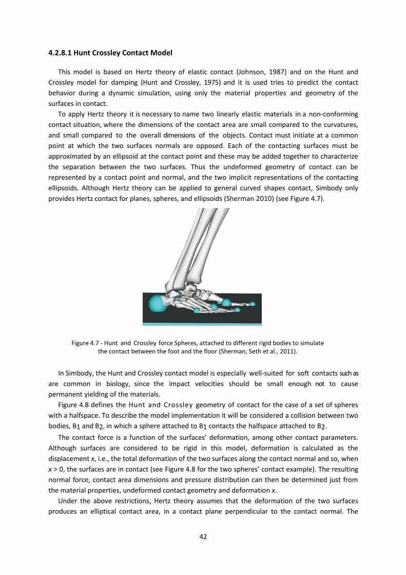
42
4.2.8.1 Hunt Crossley Contact Model
This model is based on Hertz theory of elastic contact (Johnson, 1987) and on the Hunt and
Crossley model for damping (Hunt and Crossley, 1975) and it is used tries to predict the contact
behavior during a dynamic simulation, using only the material properties and geometry of the
surfaces in contact.
To apply Hertz theory it is necessary to name two linearly elastic materials in a non-conforming
contact situation, where the dimensions of the contact area are small compared to the curvatures,
and small compared to the overall dimensions of the objects. Contact must initiate at a common
point at which the two surfaces normals are opposed. Each of the contacting surfaces must be
approximated by an ellipsoid at the contact point and these may be added together to characterize
the separation between the two surfaces. Thus the undeformed geometry of contact can be
represented by a contact point and normal, and the two implicit representations of the contacting
ellipsoids. Although Hertz theory can be applied to general curved shapes contact, Simbody only
provides Hertz contact for planes, spheres, and ellipsoids (Sherman 2010) (see Figure 4.7).
In Simbody, the Hunt and Crossley contact model is especially well-suited for soft contacts such as
are common in biology, since the impact velocities should be small enough not to cause
permanent yielding of the materials.
Figure 4.8 defines the Hunt and Crossley geometry of contact for the case of a set of spheres
with a halfspace. To describe the model implementation it will be considered a collision between two
bodies, B1 and B2, in which a sphere attached to B1 contacts the halfspace attached to B2.
The contact force is a function of the surfaces’ deformation, among other contact parameters.
Although surfaces are considered to be rigid in this model, deformation is calculated as the
displacement x, i.e., the total deformation of the two surfaces along the contact normal and so, when
x > 0, the surfaces are in contact (see Figure 4.8 for the two spheres’ contact example). The resulting
normal force, contact area dimensions and pressure distribution can then be determined just from
the material properties, undeformed contact geometry and deformation x.
Under the above restrictions, Hertz theory assumes that the deformation of the two surfaces
produces an elliptical contact area, in a contact plane perpendicular to the contact normal. The
Figure 4.7 - Hunt and Crossley force Spheres, attached to different rigid bodies to simulate the contact between the foot and the floor (Sherman, Seth et al., 2011).

43
resulting normal force, contact area dimensions, and pressure distribution can then be determined
just from material properties, undeformed contact geometry, and deformation x. The force
magnitude is
(4.19)
where R is a composite relative radius of curvature, E* is a composite elastic modulus, and 0
is an eccentricity factor with 1 for circular contact, and slowly growing as a function of elliptic
integrals of the ratio of the two relative curvatures. R and σ depend only on the curvatures of the
separation ellipsoid, so the parenthesized quantity above is independent of x. Although the materials
are assumed linear elastic, the force-displacement relationship is nonlinear because of the changing
geometry during contact (Johnson, 1987).
Figure 4.8 - Contact geometry for the Hertz/Hunt and Crossley model, for the two spheres contact example
(Sherman 2010).
To apply this force, Simbody calculates an instantaneous contact point P, located along the line
separating the initiation points on each surface, with the exact location dependent on the
relative stiffness’s of the two contacting materials (Sherman 2010). If the materials are the
same, P will be located midway between the two surfaces. If one surface is much stiffer than the
other then P will be located much closer to the undeformed surface of the stiff (non-deforming)
body than to the undeformed surface of the soft body. P determines the height of the contact patch
ellipse along the contact normal and is the center point of the contact area ellipse. The contact
31*2 2
4
3HzstifnessR E xf f

44
force is applied to each body at P along the contact normal in opposite directions, such that the
force is always pushing on each surface, never pulling (Sherman 2010).
Once the magnitude of the stiffness force has been determined as above, the Hunt and Crossley
dissipation force may be calculated as .
*3
2HC Hzf f c x (4.20)
where *c is an effective dissipation coefficient combining the individual dissipation properties of the
two contacting materials. The material property c may be determined from impact experiments as
the negated slope of the coefficient of restitution vs. impact velocity curve at low velocities, using
the relationship
1e cv (4.21)
where e is the measured coefficient of restitution and v is the impact speed. The coefficient of
restitution is not a material property. More detailed explanation on computation of c* from
individual material properties in (Sherman, 2010).
Hunt and Crossley showed that the total force
0Hz HCf f (4.22)
under typical conditions, and that negative total forces are due to un-modeled losses, not allowing
the total dissipative force to become negative
'max( )dissipation HC Hzf f f
(4.23)
This account for all contact forces in the normal direction that is
normal stifness dissipationf f f (4.24)
Finally, the friction force is calculated as follows. Find the body points coincident with the
contact point P and calculate their relative velocity v in the contact plane. With slip rate v v it is
possible to calculate the magnitude of the friction
( )friction normalf f v (4.25)
where μ represents an effective coefficient of friction that is dependent only on the slip velocity, but
is parameterized by given surface properties of the materials in contact: static, dynamic, and viscous
coefficients of friction, and a transition speed at which static friction reaches its peak value.
4.2.8.2 Elastic Foundation Model
The Elastic Foundation Model (EFM) assumes that contacting solids may be considered rigid
bodies for a thin layer of elastic material of thickness h at the surfaces. Linear elastic properties are
determined for the material properties in contact and combined into a composite stiffness modulus
E* as for Hertz contact, though with a different combining formula (Johnson, 1987; Sherman, Seth et
al., 2011)

45
The geometry of each surface, which can be arbitrarily complicated, is approximated with a
triangular mesh of suitable density. This force is only applied to contacts involving a triangle mesh,
though the object colliding with the mesh may be of any type (see Figure 4.9). Contacts which do not
involve a triangle mesh are ignored.
At the centroid of each triangle, on each surface, is placed a spring whose stiffness k can be
determined from the area of its triangle, the composite material property E* and thickness h. This
forms a “bed of springs” on the surface of each body that can be used to generate forces during
contact.
When an EFM body A contacts another body B, Simbody determines all the triangles of A whose
centroids c are inside body B, considering only undeformed geometry. For each of these
triangles, the point S on body B’s surface closest to the centroid c is determined. A displacement
x is determined as the distance from the centroid to S (see Figure 4.10). A spring is considered to
be displaced if its base location is inside the other object, and the contact point is taken to be the
nearest point on that object's surface.
Figure 4.10 – Left and Middle: Two triangular mesh spheres (A and B), in contact. Right: Contact between body
A and body B with the Elastic Foundation Contact Model: Simbody determines each triangles of A whose centroids are inside body B. S represents a point on body’s B surface, closest to a centroid c located on body’s
A polygon. A displacement x is determined as the distance from the centroid to point S, for each polygon.
Figure 4.9 - Elastic Foundation mesh-based forces for representing foot-floor contact in OpenSim (Sherman,
Seth et al., 2011).

46
Then a force kx is applied to both bodies using a contact point P along the line segment between the centroid and S. The force exerted by each spring along its displacement direction is given by
*(1 )f kax c v (4.26)
where k is the spring stiffness, a is the area of the triangular face the spring belongs to, x is the displacement distance, c is the spring's dissipation coefficient, and v the velocity along x.
A Hunt and Crossley-like dissipation term kx(*c x ) is added to complete the normal force, and
relative velocities are calculated at P and used to generate friction forces in the plane of the triangle using
( )friction normalf v f
(4.27)
If the springs are assumed to represent a uniform layer of elastic material over a rigid substrate, the stiffness is given by
(1 )
(1 )(1 2 )
p Ek
p p h
(4.28)
where E is the Young's modulus of the elastic layer, p is its Poisson's ratio, and h is its thickness.
The friction force exerted by each spring is
2
min ,1 ( 2(
.
1 .
)
normal
vsud us u
vsuv vs
vt
dvt
f f
(4.29)
where normalf is the normal force at the contact point, vs is the slip (tangential) velocity of the two
bodies at the contact point, vt is a transition velocity, and us , ud , and uv are the coefficients of
static, dynamic, and viscous friction respectively.
This is repeated independently for each overlapping triangle. When two meshes collide, the
springs on each mesh are treated independently: each mesh is assumed to be rigid for purposes of
calculating the force exerted by the other mesh's springs. If B is also an EFM body, then the same
calculation is performed for each of B’s triangles whose centroids are inside A. All force contributions
from each triangle are summed up and used to calculate the net force and moment applied to the
two rigid bodies. The distribution of normal forces is also used to calculate the center of pressure
for the irregular contact area.
EFM produces results that are inferior to the finite element method (FEM) but take much less
time to compute. In contrast to Hertz and FEM, EFM does not account for coupling between
elements and hence does not converge to the result predicted by linear elastic material theory even
at very fine mesh resolutions (Sherman, Seth et al. 2011). Despite this limitation, EFM can give very
good agreement with FEM for total force even though patch geometry may not agree as well
(Pérez-González, Fenollosa-Esteve et al., 2008).
In this work, the EFM will be used to simulate the contact between the rigid bodies, since it would
be very difficult to implement the Hunt-Crossley model given the complex geometries of the
prototypes.

47
Chapter V
Simulation Model Definition
5.1 3D acquisition of human anatomy
The lower limb model used in this work was acquired using a 3D scanner technique (Ana Luisa,
2010). This technique analyses a real-world object or environment in order to collect data on its
shape and possibly its appearance. The objective of 3D scanner is to obtain a points cloud of
geometric samples on the surface of the subject and collect distance information about surfaces, at
each point. These points can then be used to create a virtual surface, in a specific program (Ana
Luisa, 2010).
There are two kinds of scanners: Contact 3D scanners, which require physical touch and are
slower than other scanning methods, and non-contact 3D scanners that can be active (emitting and
detecting their own radiation or light) or passive (detecting reflected ambient radiation). The points
cloud produced by the 3D scanners can be used directly in some CAD software, where it can be
edited (Ana Luisa, 2010).
To obtain the points cloud it was used a non contact 3D active scanner, provided by the
Mechanics Department of Instituto Superior Técnico (IST), in Lisbon. Figure 5.1 illustrates the method
used in the application of this technique. Some marks were placed on the lower limb, as reference
points. This reference points were slowly scanned and saved to a computer in order to make the
points cloud. After the scan, the points cloud had to be edited, in order to eliminate disconnected
points that might be mistakenly introduced.
Figure 5. 1 - Left: First step on the 3D scanning, marking the reference points for the points cloud creation;
Middle: Reference points marked. Lower limb prepared to be scanned; Right: Points cloud generated after the 3D scanning. This technique often introduces some points that are not part of the scanned object, so the points
cloud needs to be edited (Ana Luisa, 2010).
5.2 Geometric Modeling of the Leg and AFO Meshes
After the 3D scan, the collected data was used to construct the 3D prototype of the lower limb
and the articulated AFO. Geometric Modeling creates 3D objects directly from a geometric database
without specific tooling or human intervention, in CAD software. This type of software use computer
technology for the process of design. SolidWorks is CAD software, based in parametric computation,

48
which makes tridimensional shapes from basic geometric shapes. SolidWorks CAD system was used
to transform the points cloud into a mesh as illustrated in Figure 5.2 (Ana Luisa, 2010).
After having the lower limb geometry (see Figure 5.2) the articulated AFO was constructed using
also SolidWorks, creating the lateral module and the plantar module of the orthosis separately. The
construction process is illustrated in Figure 5.3.
Figure 5. 2 - Creation of the lower limb geometry. Left: Points cloud obtained after the 3D scanning; Middle:
Transformation of the points cloud into a mesh, in SolidWorks; Right: Final mesh created in SolidWorks, representing the human anatomy scanned.
Figure 5. 3 - Creation of the Ankle-Foot Orthosis geometry based on the lower limb geometry.
Both geometries were used as starting point. Since one of the main goals of this work was to
simulate contact between the lower limb and the orthosis, it turned out to be necessary the creation
of other geometries to represent the straps, usually incorporated in every type of orthotic devices to
maintain the device adjusted to the patient’s body (see Figure 5.4 a). These straps were introduced in

49
the former model in order to simulate, as faithfully as possible, the patient’s condition during
walking. To create these geometries, similarly to what was done before, SolidWorks software was
used. The resulting meshes are illustrated in Figure 5.4 b)
Also, it was necessary to divide the lower limb prototype in two distinct parts to simulate the
ankle joint. The lower limb was divided at the ankle joint level resulting in two different geometries:
foot and leg (see Figure 5.5).
Figure 5. 4 - a) Articulated Ankle-Foot Orthosis with straps included that allow to adjust the AFO to the patient’s
leg (source: www.orthopedicmotion.com); b) Strap geometries, created in SolidWorks, added to the former orthosis prototype.
Figure 5. 5 - Foot and Leg geometries obtained from cutting the lower limb prototype at the ankle level. The
images were taken from OpenSim software and illustrate the foot and leg rotation about the ankle joint.
The extension files recognized by OpenSim are not the same as the extension files created in
SolidWorks being necessary to use other software to make this conversion. Also, the collision
detection algorithm used by OpenSim (see Section 4.2.8.2) assumes that only closed water-tight

50
surfaces can be used. Additionally the number of faces in the triangle meshes must not be too high,
otherwise the meshes are not recognized by OpenSim and the computational cost will be
tremendous (making that each simulation takes too long to get to the final result). The maximum
recommended number of faces for each mesh is approximately 10.000. Because some of the meshes
created in SolidWorks had more faces than the recommended, and to ensure that all the other
features were fulfilled, it was necessary to use two different softwares: Geomagic Studio 12 and
MeshLab.
Geomagic Studio 12 is a 3D software for creating digital models of physical objects and integrates
tools for rapid creation and correction of meshes. This software was used in this work as a tool to
edit and correct the meshes created in SolidWorks. Specifically, it was necessary to remove all the
spikes and holes presented in the mesh, using ‘MeshDoctor’ tool. Next, the ‘Close Manifold’ tool was
used to create a water-tight mesh. These steps were performed in all the meshes and the output files
were recorded in ‘.stl’ extension files, so they could be used in the next software: MeshLab.
MeshLab is open source software for processing and editing 3D triangular meshes. In this case,
MeshLab Decimate Filter was used to decrease the number of faces of each mesh, until the
maximum number of faces was not exceeded. With this software was also possible to align all the
meshes, using the Transform Filter that allows rotating and translating the meshes until everything is
perfectly aligned. Among all the formats available to output the data, the ‘.obj’ format is the one
required by OpenSim. At this point, the meshes were prepared to be used in the Elastic Foundation
Contact model.
5.3 Geometry Visualization Files
As mentioned above, OpenSim API is built on Simbody, which allows performing simulations of
multibody systems. As described in Chapter IV, a body defined in Simbody is just a moving reference
frame with the mass properties (mass, center of mass and an inertia tensor) associated, but with no
geometry attached. Because of this, when performing simulations with Simbody, bodies have no
geometry visualization files attached and therefore, it is not possible to visualize them in OpenSim
GUI, although their correct definition.
Hence, the geometry visualization file does not interfere in bodies’ definition. The only
contribution of the geometry file, besides the ability to visualize the body in the OpenSim GUI, is to
locate the body fixed frame as this is coincident with the origin of the geometry file created to
represent that same rigid body.
To create the geometry visualization files Paraview software was used. ParaView is an open-
source, multi-platform data analysis and visualization application, where is possible to create 3D
geometries.
In this work, the geometries were already created from MeshLab, and consequently from
SolidWorks, although in a different format. Paraview reads the ‘.obj’ files outputted from MeshLab
and convert these to ‘.vtp’ files. In this way, the geometry visualization files will match the geometry
meshes, which will be necessary to implement the contact model. The only modification necessary to
perform in the ‘.vtp’ files was to redefine their origin. Figure 5.6 illustrates the bodies and their origin
location defined in Paraview. Note that the reference axes notation in Paraview is the same as in
OpenSim.

51
Figure 5. 6 - The individual origin location for the six bodies defined in the multibody system. By choice, the
origin of all the bodies was placed at the same location, coincident with the ankle joint.
5.4 Mass Properties
The mass properties needed to define a body in Simbody include: mass, center of mass and the
moments of inertia.
The calculations for leg and foot mass were based on the work of Winter, illustrated in Table 5.1
(Winter 1991). Knowing the total weight of the person whose leg was scanned (Ana Luisa, 2010) the
masses for both foot and leg were calculated as follows:
Foot Total
Leg Total
M = 0.0145*M = 0.0145*72Kg=1.044Kg
M = 0.0465*M = 0.0465*72Kg=3.348Kg (5.1)
Since the AFO prototype model was actually manufactured (Ana Luisa, 2010), the AFO elements
were weighed and the individual masses obtained:
_
_
M = 0.170Kg
M = 0.320Kg
M 0.020
Down part
Up part
Straps Kg
(5.2)
OpenSim uses the SI convention (length in meters; mass in kilograms; time in seconds; forces in
Newton; and moments/torques in Newton.meters). Angles can be in degrees or radians; internally,

52
OpenSim uses radians. Also, the center of mass and moments of inertia are defined with respect to
the body’s local reference frame, located on the body itself which is coincident with the origin of the
body’s geometry file defined in Paraview. Taking this into account, the values for the center of mass
and inertia were taken from SolidWorks and the coordinates were calculated as the distance
between the center of mass given by SolidWorks and the origin of the reference frame, coincident
with the origin reference frame defined in Paraview. The coordinate values for the center of mass of
the six rigid bodies follow:
_
_
C
C
C
C
= (0.00183, 0.17849, -0.02869) [m]
= (0.03524 , -0.03765 , -3.22) [m]
= ( 0.02226, -0.06392, -0.00885) [m]
= ( -0.01364, 0.17797, 0.00692)
MassLeg
MassFoot
MassDown part
MassUp part
r
r
r
r
_
_
C
C
[m]
= ( 0.13192, -0.04731, 0.00307) [m]
= ( 0.05025, 0.26411, 0.00265) [m]
MassFoot Strap
MassLeg Strap
r
r
(5.3)
The principal moments of inertia for each body were calculated in SolidWorks, relative to the
bodies’ center of mass. Since Simbody expects these values to be given relative to the bodies’ local
fixed frame it was necessary to apply the Parallel axis theorem (or Steiner Theorem). The parallel axis
theorem says that given the body's moment of inertia, about a parallel axis through the object's
centre of mass, and the perpendicular distance r between the axes, the moment of inertia about new
axis is given by:
2
z cm= +mI I r (5.4)
Hence, the principal moments of inertia, (Ix, Iy, Iz) obtained for each body were:
(5.5)
Leg
Foot
Up_part
Down_part
2
o
-4 2
o
2
o
-4 -4 2
o
= (0.024, 0.111, 0.027) [Kg.m ]
= (0.002, 0.005, 3.542x10 ) [Kg.m ]
= (0.0032, 0.0113, 0.0025) [Kg.m ]
= (2.033x10 , 0.0012, 4.423x10 ) [Kg.m ]
I
I
I
I
Foot_Strap
Leg_Strap
-5 -5 -6 2
o
-5 -5 2
o
= (3.685x10 , 6.192x10 , 6.376x10 ) [Kg.m ]
= (5.965x10 , 0.0014, 2.954x10 ) [Kg.m ]
I
I

53
5.5 Defining Mobilizers between the Bodies
Chapter IV describes how bodies in a Simbody multibody system connect with each other. In
Simbody, a multibody system is represented as a multibody tree of interconnected bodies, where
Ground (body 0) represents the root. Bodies are connected to a parent body through a mobilizer,
which provides mobility between this and the body. Table 5.2 illustrates the types of mobilizers used
between the different bodies and the ground.
Table 5. 2 - Bodies and mobilizers used to connect these to their parent bodies.
Body Mobilizer Parent Body
Leg Free
Ground
Table 5. 1 - Anthropometric Data (Winter, 1991).

54
Foot Torsion
Leg
Lateral Module
Free
Ground
Plantar Module
Torsion
Lateral Module
Leg
Strap Weld
Lateral Module
Foot
Strap Weld
Plantar Module
5.6 Defining Contact Between the Multibody System Bodies
In section 4.2.8 the two contact models provided by Simbody were described. In this work, the
Elastic Foundation contact model is used instead of Hunt-Crossley model.
Hunt Crossley contact model proved to be less accurate and more difficult to implement, given
the irregular geometry of the prototypes. In addition, it would be necessary to define too many
contact spheres in order to simulate a real contact between the bodies, and the computational cost
of this implementation would be enormous and time consuming (see Section 4.2.8.1).
Since the meshes for all the bodies defined in the multibody system were already created in
SolidWorks, the Elastic Foundation model proved to be the most consistent choice, in order to obtain
results closer to reality and more accurate in terms of distribution of forces. Hence, after assigning all
the meshes to the respective bodies creating the contact geometries, it was necessary to define the
different pairs of contact. In order to study the contact forces between the lower limb and the AFO,
the following pairs of contact were defined: a contact force between the foot and the plantar module
of the orthosis prototype; a contact force between the foot and the Foot Strap; a contact force

55
between the leg and the Lateral module of the AFO; a contact force between the leg and the Leg
Strap (see Figure 5.7).
Figure 5. 7 - Definition of the different contact forces existing in the model: Only the contact forces between
the pairs of contact of interest to this work were defined.
Equation 4.28 represents the stiffness, k, for the Elastic Foundation contact model. From the
literature, it was founded that the Young’s modulus and Poisson’s ratio for human flesh is E = 50 kPa
and ν=0.36, for human bone is E = 9 GPa and ν=0.4 and for Polyvinyl Chloride (PVC) is E = 3.4 GPa and
ν=0.36 (Creations; Leon Bennett; Beer, Junior et al., 2006). With these values, the stiffness for each
pair of contact was calculated, opting to consider the material with the lower stiffness for its
calculation. Hence, the stiffness values obtained for a 1mm thickness (h) were:
3
3
3
93
3
93
3
(1 0.36)(50 10 )1.78 8 (N.m )
(1 0.36)(1 2*0.36)(1*10 )
(1 0.4)(9 10 )4.5 13 (N.m )
(1 0.4)(1 2*0.4)(1*10 )
(1 0.36)(3.4 10 )1.21 13 (N.m )
(1 0.36)(1 2*0.36)(1*10 )
Flesh
Bone
PVC
xk e
xk e
xk e
(5.1)

56
To store the net resultant contact forces in a *.mot file, the ForceReporter analysis was used,
allowing to record not only the net resultant contact forces defined, but also other prescribed forces
applied to the model, during the simulation.
5.7 Prescribed Motion
This section describes how the kinematic and kinetic experimental data were acquired as well as
the calculations necessary to obtain the joint angles and trajectories necessary to prescribe a non-
pathological gait movement to the system. Ahead, the calculations necessary to obtain the ground
reaction forces values and to convert the kinetic data from the action-oriented coordinate system to
OpenSim’s coordinate system are explained.
5.7.1 Experimental Kinematic Data Acquisition
The experimental kinematic data was acquired in the Lisbon Biomechanics Laboratory (LBL). The
acquisition of kinematic data was made by means of eight IR cameras – Qualisys ProReflex and the
acquisition software used was Qualisys Track Manager (QTM) (QUALYSIS 2010). The markers used in
the trials were spherical passive markers with flat base and 19mm of diameter. They were made of
polystyrene hemispheres covered in special retro-reflective tape. (Gonçalves 2010).
The total number of markers used was 14, distributed along the lower limbs (7 markers in each).
The distribution of the left lower limb markers is illustrated in Figure 5.8: two markers were placed
around the knee, on the medial and lateral side; two markers were placed on the ankle, one at the
lateral side and another one on the medial side. One marker was placed on the heel, and the
remaining two markers were placed on the II and V metatarsal head. Two markers were used in the
ankle and knee joints because this enables an easy and more precise determination of the articular
center of those joints, by computing the medial point of the two markers (Gonçalves 2010).
Figure 5. 8 - Marker set protocol: markers in anterior view (left) and lateral (right) view.
QTM was used to acquire the markers positions and treat the trajectories. The Initial Contact (left
foot) was chosen as the first event. Depending on the stride to be analyzed (right or left), one should
consider at least 10 frames before the IC of the foot in analysis and at least 10 frames after the

57
second IC of the same foot (Gonçalves 2010). This measure is essential to a correct data filtering.
Kinematic data was then exported to a *.tsv file. In order to filter data and change from the QTM to
OpenSim reference frame (see Figure 5.9) it was necessary to develop some routines in MatLab. The
data was filtered with a 3rd order low pass digital Butterworth Filter with a cutoff frequency of
0.16Hz.
Figure 5. 9 - Reference frames in QTM and OpenSim are not coincident. In order to have the kinematic data
consistent with the OpenSim reference frame it was necessary to make the equivalent changes.
5.7.2 Determining Joint Angles
In gait analysis, human body segments are generally modeled as rigid bodies and their rotation is
assumed to take place about a fixed point in the proximal segment, which is considered to be the
center of the joint. Euler angles have been successfully applied to describe a relative rotation of one
segment with respect to another segment in 3D space (see section 4.2.3). Other methods can be
used, for example Lewis and Lew defined the orthopedic angles that are the same as Euler angles but
they are defined according to the clinical terms (flexion, extension, abduction, among others)
(Kadaba, Ramakrishnan et al., 1990).
The joint angles definition used in this thesis follows the convention of Winter and the
International Society of Biomechanics. Winter states that all segments must be defined as positive in
a counter-clockwise direction from the horizontal in order that the first and second time derivatives
have the correct polarity for subsequent kinetic analyses (energy, moment of force and power). Thus,
the joint angles have a positive value if these are in dorsiflexion and negative value if these are in
plantar flexion (Winter 1991).
In the sagittal plane, it is assumed that the right side of the subject is being viewed as he
progresses from left to right. Angles reported for the left limb should have the same convention as
the right limb, in order to allow the direct comparison between the results of the two legs. According
to Winter (see Figure 5.10) the sagittal angles for the lower limb are defined as follows:
- Foot Angle (θft) – the angle between the horizontal and a line along the bottom of foot
measured for the distal end (V metatarsalphalangeal joint).
- Leg Angle (θlg) – represents the angle between the horizontal and the line defined by knee
joint and ankle joint measured from the distal end of leg (ankle joint).
- Thigh Angle (θth) – is the angle between the horizontal and the line defined by the thigh (hip
joint to knee joint) measured from the distal end of thigh (knee joint).

58
- Pelvic Tilt – represents the angle between a horizontal line and the pelvis (line between PSIS
iliac and the ASIS)
- Trunk Angle (θtr) – represents the angle between the horizontal and the line defined by the
axis of spine (C7 to L5)
- Ankle Angle (θa) – represents the angle between the foot and the leg minus 90º. (θa=θft-θlg-
90º)
- Knee Angle (θk) – represents the angle between the thigh and the leg. (θk=θth-θlg)
- Hip Angle (θh) – is the angle measured between the thigh and the trunk. (θh=θth-θtr)
To calculate the leg ankle angle for the kinematic data acquired, some routines in MatLab were
developed. Figure 5.11 illustrates the results obtained from those calculations, which are consistent
with the literature (Winter 1991).
Figure 5. 10 - Definition of joint angles of lower limbs in sagittal plane (Winter 1991).

59
Figure 5. 11 - Joint angles obtained for the leg (top) and the ankle (bottom).
5.7.3 Trajectories
For every mobilizer defined in OpenSim, it is possible do define a CoordinateSet representing all
the DOF allowed by that mobilizer. For example, if we define a Free mobilizer between two bodies,
the CoordinateSet will represent the six DOF allowed by the Free Mobilizer: three rotations and three
translations along the x, y and z axes. For Torsion mobilizer there will be only one DOF allowed
between the two bodies. In this case the CoordinateSet, by default, will define only one rotation
along the z axis.
OpenSim also enables the setPrescribedFunction which receives as an input a function of time and
will apply that function to a "coordinate" rather than to a "body". If a body is attached to another
using a mobilizer, that has multiple coordinates (defined by the CoordinateSet) and it is possible to
specify a different function for each coordinate.
One of the objectives of this work was to prescribe a non-pathological gait movement to the
system in order to study the interface contact forces developed between the surfaces. This section
explains how the movement can be prescribed to the leg and foot sub-system.
As described in Section 5.5, the Leg is connected to the Ground Body with a Free Mobilizer and
the Foot is connected to the Leg by a Torsion Mobilizer. This means that, in order to prescribe any
movement to the Leg-Foot system, it will be necessary to specify the six degrees of freedom of the
Free mobilizer and the unique degree of freedom of the Torsion mobilizer (between the Foot and the
Leg).

60
By default, the orientations in OpenSim are described using body-fixed X-Y-Z Euler angles and the
translational coordinates are given about the body’s local reference frame. One would expect that
the trajectories of the kinematic data obtained in section 5.7.1 corresponded to the trajectories
necessary to prescribe the translations, over time, in the three axes x, y and z. However, by default,
the translational coordinates represented by the CoordinateSet represent the coordinates in the
body's local frame, instead of representing the coordinates in the inertial frame (Ground reference
frame) (see Figure 5.12).
Through Equation 4.5 it was possible to deduce the Euler angles (Ψ, θ, σ) corresponding to the x, y
and z orientations of the leg’s body, for each time step. Since the trajectory vector with coordinates
(x, y, z) expected by OpenSim is given in the body’s local frame, r’, it was necessary to calculate the
values for this vector using the trajectory vector r, given by the experimental kinematic data, and the
body’s rotation matrix. Using Equation 4.5, that represents the general rotation matrix of the
individual rotations about the x, y and z axes, respectively, the r’ values were obtained by multiplying
the r vector and the correspondent inverse matrix of Equation 4.5:
' ' -1 = =r Ar r A r⇔ (5.2)
To systematically perform these calculations some MatLab routines were developed and after
calculating the r’ vectors, the NaturalCubicSpline function was applied in order to obtain the
trajectories interpolation along the x, y and z axes individually as a function of time.
Figure 5. 12 - Representation of body B and its Inertial frame trajectory vector, r. To translate body B from a
point P1 to a point P2 OpenSim expects to be given the body’s local frame trajectory vector, r’, instead of vector
r, as it would be expected.
Assuming that the ankle is stabilized and that there is only rotation along the medial-lateral
direction, the unique DOF allowed by the torsion mobilizer was prescribed using the ankle angles (θa)
of Winter’s definition (see Figure 5.10).

61
5.7.4 Ground Reaction Forces
The reaction force generated from the contact between the orthoses and the ground is the
ground reaction force (GRF), which is basically the reaction to the force the body exerts on the
ground. The GRF is measured by the force plate.
The GRFs were acquired in the LBL with three AMTI-OR6-7 force platforms (508mm x 464mm).
Since the data yielded by the force plates represents voltage, it was necessary to use some MatLab
routines in order to obtain the corresponding forces and moments of force in Newton. The spatial
arrangement of the force plates used is represented in Figure 5.13.
Figure 5. 13 - Representation of arrangement in space of the eight IR cameras (red) used to acquire the
motion and the three force plates used to acquire the ground reaction forces (GRF) during the stride period (white) (Based on (Gonçalves 2010).
The AMTI force plates use the action-oriented coordinate system (see Figure 5.14a)). According to
Kwon, the reference used to calculate the GRF should be the reaction-oriented coordinate system so
it was necessary to convert one reference to the other (see Figure 5.14b)) (Kwon, 1998).

62
Figure 5. 14 - Conversion from action-oriented coordinate system (left) to reaction-oriented coordinate system (right).
To convert the data from the action-oriented system to the reaction-oriented system it is necessary to change the sign of the components of the GRF and moments, like described above:
x x' x x'
y y' y y'
z z' z z'
'
'
'
F F M M x x
F F M M y y
z zF F M M
(5.3)
All the forces acting between the foot and the ground can be summed to yield a single ground
reaction force vector and a free torque vector. The point of application of the ground reaction force
on the plate is the center of pressure (COP). The Z component of the COP position is always 0.The
moment measured from the plate is equal to the moment caused by F about the true origin of the
force plate, thus:
' '' '
' ' ' '
' ' ' '' '
( )0 0
0 ( ' ) 0 ( )
( ' ) 0 ( ) ( )
z yx x
y y x z
z y x zz z
y b F cFM Fc y b
M c x a F cF x a F
y b x a T x a F y b F TM F
(5.4)
According to Equation 5.4 is it possible to determine the x and y values of the COP for each plate:
' '
'
'
' '
'
' ' ' '
COP
COP'
( ' ) ( )
y x
x
z
x y
y
z z y x
M cFa
F
M cFb
Fz
T M x a F y b F
(5.5)
where (a,b,c) corresponds to the true origin of each force plate, which can be found in the calibration
data sheet.

63
Because it is necessary to combine the ground reaction force data with the kinematic data
obtained through motion analysis and because the GRF are prescribed to the model in the
simulation, it was essential that the reference frame was the one according to OpenSim reference
frame. In order to achieve that, another conversion had to be made from the reaction-oriented
coordinate system to the OpenSim coordinate system (see Figure 5.15).
Figure 5. 15 - Conversion from reaction-oriented coordinate system (left) to OpenSim coordinate system (right).
Again, the data had to be converted from one coordinate system to another. Please note that in
this specific case, the foot under analysis corresponds to the left-foot which, according to the
acquisition reference frame, causes a rotation of 180o around the Y axis. So, the conversion from the
force-plate reaction reference frame to the OpenSim reference frame had to be as followed:
x'' y' x'' y'
y'' z' y'' z'
z'' x' z'' x'
'' '
'' '
'' '
F F M M x y
F F M M y z
z xF F M M
(5.6)
Also, according to Figure 5.13 and Equation 5.5:
'' '
'' ''
'' '
'' '
'' '
''
0.508 COP COP
2Force Plate 1
0.464 COP COP
2
0.508 COP (0.1 ) COP
2Force Plate 2
0.464 COP (0.1 ) COP
2
3*0.508 COP 0.1 COP
2Force Plate 3
COP (0.1
x y
y x
x y
y x
x y
y
'
0.464) COP
2
x
(5.7)
After performing all the necessary changes, the values for the components of the COP and GRF
were obtained according to the OpenSim reference frame (see Figure 5.16; Figure 5.17; Figure 5.18;

64
and Figure 5.19) and were in line with the expected values (Perry, 1992). To remove the residual
noise from the data a Butterworth filter was applied with a cut-off frequency of 20Hz. Figure 5.16 to
Figure 5.19 shows the graphics for the filtered data. To systematically perform these calculations
some MatLab routines were used as well and, after calculating the components for the GRF,
moments and COP coordinates, the NaturalCubicSpline function was applied in order to obtain the
trajectories interpolation along the x, y and z axes individually as a function of time. OpenSim
enables a function called PrescribedForce which prescribed these values to a body in the defined
system. The GRFs were applied to the plantar module of the orthosis.
Figure 5. 16 – Ground Reaction Forces in the antero-posterior axis.
Figure 5. 17 – Ground Reaction Forces in the vertical y axis.

65
Figure 5. 18 – Ground Reaction Forces in the medial-lateral z axis.
Figure 5. 19 - COP values in the antero-posterior axis (left) and medial-lateral axis (right). Please note that the vertical component of the COP is zero, at any instant.
5.8 Running the Simulation
After the simulation file is prepared it is necessary to run the simulation. The OpenSim model is
saved into a *.osim file, which will allow to visualize the model in the OpenSim GUI. The motion file
will be saved in a *.mot file that can be loaded in the OpenSim GUI and added to the model in order
to visualize the model performing the prescribed motion. Also, a *.mot file will be created, resulting
from the ForceReporter function, which records the Forces applied to the model during a simulation.
To run the simulation, two different softwares were required: Cmake and Visual Studio C++.s
Cmake is an open-source build system that creates software build systems for a wide variety of
platforms being, basically, a “makefile maker”. It is used to control the software compilation process
using simple platform and compiler independent configuration files, generating native makefiles and
workspaces that can be used in the compiler environment of one’s choice (Visual Studio, in this case).
A simple CMake project will need only a single CMakeLists.txt control file and the source code. In this

66
case, a CMakeLists.txt was defined referring to the C++ code created. Visual C++ Studio is the
development environment for creating Windows applications. It has tools for developing and
debugging C++ code, especially code written for the Microsoft Windows API. This software will be
necessary to build and compile the C++ code developed.
After running Cmake a *.sln file is generated. After launching Visual Studio, the *.sln file is loaded
and it is possible to compile and run the program to create the files needed in the OpenSim GUI.

67
Chapter VI
Results
6.1 Computational Simulations
In this section, the results of several computational simulations are shown and discussed. The
biomechanical simulation model developed was used to simulate two distinct situations. In the first
situation, all the DOF of the lower limb sub-system were prescribed using the experimental kinematic
and kinetic data of a normal gait acquired in the gait laboratory, as described in section 5.7. The DOF
of the orthosis sub-system were left free, in order to analyze its response to the leg’s movements
and the contact forces generated. With this simulation it was intended to simulate the behavior of
the orthosis prototype as a passive orthosis. Passive orthoses do not help in the movement of the
limb, just immobilize or limit the activity of one or more joints due to a muscle imbalance and
thereby correcting improper positioning of the limb.
For the second situation, no rotational angles were prescribed to the ankle’s joint, allowing the
foot to move free simulating the absence of muscle strength in the foot. Instead, the rotational
angles used in the previous situation to prescribe the ankle’s joint were prescribed to the orthosis
joint, in order to correct the foot movement through the orthosis action. In this second simulation it
was intended to simulate an active orthosis prototype, i.e., that assists the movement of the foot.
Active AFOs are devices used to increase the ability of persons suffering from foot pathologies by
augmenting power at the AFO joint.
The contact between the lower limb and the orthosis prototypes was defined through several
pairs of contact, using the Elastic Foundation contact model (see Section 5.6).
Figure 6. 1 - Simulations kinematics obtained for the two distinct situations. Top: lower limb DOF prescribed with experimental kinematic data and GRF applied to the plantar module of the orthosis. Bottom: leg DOF prescribed and ankle joint left free for rotational movement. Orthosis joint prescribed with the same kinematic as for ankle joint in the first situation. GRF also applied to the orthosis’ plantar module.

68
All simulations were performed in a forward dynamic analysis perspective where some of the
degrees of freedom of both sub-systems, depending on the situation, were prescribed. In the
acquisition made in the laboratory, the Initial Contact of the left foot was chosen to be the first
event. Figure 6.1 illustrates the kinematics obtained for both simulations. The observation of these
two movements reveals that the kinematic is consistent with the normal gait movement described in
Section 2.3.
The kinetic data used was the same for all the simulations and was always applied to the plantar
module of the orthosis.
Ground reaction forces can be represented as a single vector that combines vertical, sagittal and
coronal forces, whose slop is equivalent to the ratio of the vertical force to horizontal shear present
(Perry, 1992). Figure 6.2 illustrates the GRF vector applied to the plantar module of the orthosis. The
images were taken from OpenSim’s GUI.
Figure 6. 2 - Ground reaction forces represented as a single vector that combines, simultaneously, vertical,
sagittal and coronal forces.
OpenSim provides no information about the values of individual contact forces developed on each
mesh polygon, allowing only knowing the values for the resultant contact forces for each time step of
integration. In addition to this limitation, OpenSim also does not provide information about the
application points for these resultant contact forces. This limitation of software represents a barrier
in the analysis of the results.
Besides not being able to know the contact force distribution along the surfaces, which was the
intended, it was not possible to infer about the resultant contact forces point of application, i.e.,
where the contact forces are being most applied, since OpenSim also does not provide this
information. For this reason, in order to visualize these forces in OpenSim’s GUI, it was chosen to
represent the resultant contact forces on the bodies’ center of mass, though this does not
correspond to reality. The discussion of results will be based on these values, for each pair of contact
established.
In order to compare the resultant contact forces values with the different MFT values tolerated by
the lower limb, some critical points of analysis were determined and their approximate values for
PPT and MFT established, based on Figure 3.8 and Table 3.1.

69
The location of points 1, 2, 3 and 4 (see Figure 6.3) correspond to the exact location of the points
2, 3, 7 and 8 in Figure 3.8, therefore the same values of PPT were assigned for these points:
545.5kPa, 588.1kPa, and 557.7kPa 416.6kPa respectively. For the PPT value of point 5 (see Figure
6.3), located at the dorsal foot, it was assigned the value of the nearest point in terms of location
(point 1 in Figure 3.8): 281.7kPa. Point 6, located in the heel (see Figure 6.3), corresponds to a very
sensitive area therefore, since there isn’t an exact match to its location, the lowest PPT value of the
highest sensibility group (see Table 3.1) was assumed: 281.7kPa. Similar, point 7, located in the
plantar foot (see Figure 6.3), was considered a point of high sensibility, considering the lowest value
of PPT of the highest sensibility group (see Table 3.1): 281.7kPa.
Figure 6. 3 – Critical points for analysis of PPT defined for the lower limb prototype.
In order to calculate the MFT, the surface areas of the orthosis prototype were obtained through
SolidWorks software:
(7.1)
Based on the values of PPT considered by Belda-Lois et al. and the area of each surface, the values
of MFT were calculated. These values correspond to the maximum load that each of the points may
be subject, taking into account the areas of each element of the orthosis in contact with the lower
limb. Table 6.1 illustrates the PPT and MFT values obtained for each defined point.
2
2
2
2
A 0.1105 m
A 0.0315 m
A 0.0105 m
A 0.0062 m
Up Part
Down Part
Leg Strap
Foot Strap

70
Table 6. 1 - Points of pressure sensibility in the lower limb prototype.
Body
Part
Anatomical
Point
PPT
[kPa]
MFT
[kN]
Orthosis surface in
contact
Leg (anterior) P1 545.5 51.95 Strap
Leg (anterior) P2 588.1 56.01 Strap
Leg (posterior) P3 557.7 5.05 Lateral Module
Leg (posterior) P4 416.6 3.77 Lateral Module
Foot (dorsal) P5 ≈281,7 ≈45.44 Strap
Foot (heel) P6 ≈281.7 ≈8.94 Plantar Module Foot (plantar) P7 ≈281.7 ≈8.94 Plantar Module
Figure 6.4 shows the contact forces exerted by the lateral module of the orthosis on the leg for
both simulations. The results show that contact occurs mostly during the stance period, i.e.,
approximately 60% of the gait cycle. For the swing period, since there are no forces applied to the
orthosis neither to the lower limb and the orthosis is suspended on the lower limb during this phase,
the contact forces are low and stable during the entire period.
Analyzing the magnitude of the forces between the lateral module of the orthosis and the lower
limb for both simulations, it is possible to notice that the contact forces in the medial-lateral
direction (z axis) are higher than the expected. These interface forces might be due to the application
point of the GRF, to the 3D geometry of the models, or both simultaneously.
If the application point of the GRF is too deviated from the medial axis of the plantar module of
the orthosis, the binary caused by these forces tend to rotate the orthosis causing high lateral
contact forces between the lateral module of the orthosis and the lower limb, since there is no
complacency of the orthosis.
A mismatch between the geometry of the two sub-systems will mean that when prescribing the
experimental kinematic data, the lower limb will move and its rotation axis will misalign with the
orthosis rotation axis. Because of the constraints imposed to the degrees of freedom of the ankle
joint and the orthosis joint, the two 3D prototypes cannot accommodate to each other causing high
contact forces between the geometries. If both are contributing for these elevated values, this means
that the application point of the GRF forces is also causing misalign in both models geometry and
therefore, the interface forces are high when in fact that does not happen in reality.

71
Figure 6. 4 – Contact forces between the leg and the lateral module of the orthosis (normalized by body mass).
Top: results for the passive orthosis simulation; Bottom: results for the active orthosis simulation.

72
To study the origin of these high interface forces another simulation was performed to test these
hypotheses. In this new simulation only the kinematic data was prescribed to the model, in order to
see if the magnitude of the interface forces remains high even without the prescription of GRF. If so,
one may conclude that the cause will be related to the model’s geometries incompatibility, given the
kinematic data. If not, then probably the problem is associated with the GRF and their application
point.
The results of the new simulation are illustrated in figure 6.5. For the contact forces between the
lateral module and the leg, in both situations (passive and active orthosis), it is clear that there was a
decrease in the forces in the medial-lateral direction, as well as in the other directions, although
there is still some high frequency oscillating movement.
Figure 6. 5 - Contact forces between the leg and the lateral module of the orthosis (normalized by body
mass). Left: results for the passive orthosis simulation with no kinetics prescribed; Right: results for the active
orthosis simulation with no kinetics prescribed.
Figure 6.6 illustrates the contact forces between the plantar module and the foot for the passive
and active orthosis simulation. Looking to the graphic, it is possible to recognize the pattern of the
GRF in the vertical direction (applied to the plantar module of the orthosis) during the stance phase.
In the progression direction (x axis) the interface forces are probably due to the GRF components in
this direction. In the medial-lateral direction the oscillatory movement is almost nonexistent.
During the swing phase there is no external loads applied and the orthosis is suspended on the
lower limb and therefore, the small interface forces obtained during this period are in agreement
with the expected results.
Also for this case, the new simulation with no kinetics prescribed was performed, in order to
study the influence of the GRF on the forces magnitude. Figure 6.7 illustrates the results obtained for
this simulation in both situations (passive and active orthosis). The results show that also for this
case, no significant contact forces occur during the entire movement since the foot is well
accommodated to the orthosis and there is no forces applied to the plantar module of the orthosis,
although there is a small increase in the forces in the x and y direction in the Terminal Swing phase,
probably due to the extending movement of the knee which causes the sliding of the plantar module
of the orthosis on the foot.

73
Figure 6. 6 - Contact forces between the foot and the plantar module of the orthosis (normalized by body mass). Top: results for the passive orthosis simulation; Bottom: results for the active orthosis simulation.

74
Figure 6. 7 - Contact forces between the foot and the plantar module of the orthosis (normalized by body
mass). Left: results for the passive orthosis simulation with no kinetics prescribed; Right: results for the active orthosis simulation with no kinetics prescribed.
Through the results obtained it is possible to conclude that probably the application points of the
GRF are causing high contact forces between the lateral module and the leg, which do not
correspond to reality. This problem could be solved if the acquisition of experimental kinematic and
kinetic data was performed by a subject with an orthosis instead of a barefoot subject, since the
forces and centers of pressure recorded for a normal subject walking barefoot are different from the
forces and centers of pressure recorded with a normal subject wearing an orthosis or a shoe.
The straps function, for every orthotic device, is adjusting the orthosis to the body preventing
undesired movements of the orthosis relative to the body. This adjustment is called pre-tightening
and represents a deformation of the skin tissue and the strap, resulting in interface forces between
the surfaces. The pre-tightening is a very important parameter, since it is responsible for preventing
relative movement between the surfaces that could cause skin irritation and lead to discomfort
although, if the pre-tightening is excessive it will provoke high deformations on the skin tissue and
consequently high interface forces that could also lead to discomfort.
In this model it was not possible to set a pre-tightening because this would imply to previously
overlap the meshes of the 3D prototypes. Using OpenSim and the Elastic Foundation model, the
calculations for 3D models with overlapping meshes would result in very high contact forces that
would not correspond to reality. Instead of setting a pre-tightening, the adjustment of the straps
mesh and the lower limb mesh was made as tight as possible. Although this previous adjustment, a
small gap between the straps and the lower limb was left, in order to avoid the overlapping. Ideally
this would never happen because the straps are usually made of an elastic and adjustable material.
Even if a pre-tightening was defined between the straps and the limb interface, there would still be
oscillating movements between the orthosis and the lower limb since the orthosis is also not
completely adjusted to the leg. This issue is one of the major problems for no-customizable orthotic
devices, and is one of the main reasons leading to discomfort in AFOs design.
For this model, the straps behave like rigid and undeformable bodies, although currently they are
usually made of deformable materials. Therefore, this rigid behavior might cause an increase of
magnitude of the interface forces obtained.

75
Figure 6. 8 - Contact forces between the leg and the strap (normalized by body mass). Top: results for the
passive orthosis simulation; Bottom: results for the active orthosis simulation.

76
Figure 6.8 illustrate the results obtained for the strap adjusting the orthosis to the leg in both
situations (passive and active orthosis). Analyzing the graphic in Figure 6.8 for the passive orthosis
case it is possible to visualize that the most relevant forces occur during the stance period, with a
peak in the weight acceptance phase. The oscillatory movements in the vertical and medial-lateral
directions are caused by the relative movement between surfaces, which could be easily corrected if
a better mesh adjustment could be made. During the swing phase the results suggest that there is no
contact between the strap and the leg, probably due to the absence of pre-tightening between them.
For the active orthosis case, there is a higher oscillation movement between the orthosis and the
leg during the swing phase, caused by the ankle joint instability and the inability of the ankle joint to
keep the neutral position, tending to flex the foot.
Figure 6.9 represents the contact forces for the foot strap, in both situations. It is possible to see
that for the case of simulation of a passive orthosis the interface forces between the foot and the
strap follows the pattern of the forces between the plantar module and the foot, although in
negative direction. During the swing phase there were no interface forces between the straps and
the lower limb, probably due to the lack of pre-tightening.
For the active orthosis, there is a peak coincident with the Pre-swing phase which might also be
caused by the ankle joint instability. These results suggest that the normal kinematic data prescribed
to the orthosis might not be enough for it to control the foot during the gait movement although, in
practice, the usage of shoes help the foot to accommodate the orthosis and also helps the orthosis to
stabilize the foot movement.
For both simulations the most significant contact forces occur during the weight acceptance/
onset of mid stance phase. For the plantar module and the foot strap, the most significant forces
occur in the vertical axis and followed the GRF pattern due to the kinetic prescription of GRF applied
to the plantar module of the orthosis.
In terms of comfort/discomfort of the subject, the maximum force values obtained were
compared to the MFT values of table 6.1. All contact forces developed are below the MFT values of
the corresponding critical points (see Table 6.2). For the active orthosis, the contact forces developed
were significantly higher. This is due to the fact that the work necessary for the orthosis to control
the leg is higher than the work done by the leg to control the orthosis, since the orthosis modules are
much lighter than the lower limb.
Although these results suggest that the forces developed by the orthosis prototype are not
enough to cause discomfort, the results showed some high frequency oscillating movements
occurring that could lead to skin irritation and to the patient’s discomfort. These oscillating
movements between the orthosis and the lower limb might be suppressed by the proper adjustment
and pre-tightening of the straps and also by the orthosis proper design and subject customization.
Please note that the dissipation coefficient considered for these simulations was 0.9 in a scale from 0
to 1.

77
Figure 6. 9 - Contact forces between the foot and the strap (normalized by body mass). Top: results for the
passive orthosis simulation; Bottom: results for the active orthosis simulation.

78
Table 6. 2 – Comparison of the contact forces maximum values with the MFT values established
Body
Part
MFT
[N/Kg]
Passive Orthosis
Maximum Force
[N/Kg]
Active Orthosis
Maximum Force
[N/Kg]
Orthosis part
in contact
Leg (anterior) 721.53 (P1) 777.92 (P2)
x axis: 3
x axis: 1.1
Leg Strap y axis: 1
y axis: 1.1
z axis: 1
z axis: 0.4
Leg (posterior) 70.14 (P3) 52.36 (P4)
x axis: 1.5
x axis: 8
Lateral
Module
y axis: 3.5
y axis: 3
z axis: 13
z axis: 9
Foot (dorsal) 631.11 (P5)
x axis: 20
x axis: 90
Foot Strap y axis: 45
y axis: 200
z axis: 12
z axis: 43
Foot (heel) 124.17 (P6) 124.17 (P7)
x axis: 20
x axis: 8
Plantar Module
y axis: 55
y axis: 18
z axis: 4
z axis: 4.5

79
Chapter VII
Conclusions and Future Developments
7.1 Conclusions
Ankle foot orthoses design and materials have suffered a tremendous evolution since its first
appearance. AFOs are prescribed for several conditions like stroke, cerebral palsy, spina bifida,
multiple sclerosis, paraplegia, polio, ankle and foot deformity or fractures. Therefore, there are a
variety of ankle foot orthoses available, depending on the diagnosis and physical needs of the
individual.
Ankle foot orthosis design can and should be altered to save weight, improve functional
properties, be more suitable and patient customized, since all patients differ in terms of
anthropometric features.
Researchers begin to apply engineering methodologies and techniques in the manufacture of
orthoses, as opposed to almost artisan manufacturing techniques previously used. However, most of
the research work has not taken into account the patient/orthotic device interface, although
orthoses can be highly customized through the incorporation of surface pressure measurement
analysis into the design process.
There is little information on this subject, and each case is unique since all patients respond
differently to each orthotic devices, either because of different anthropometric features, because of
the orthosis design and material used or because they have greater or no sensibility at all, depending
on the pathology. An ankle-foot orthosis should provide the patient the ability to recover his
biological function of the lower limb, without experiencing discomfort. This issue is directly related
with the interface forces developed in the patient/orthotic device interface.
The main objective of this work was to develop a simulation model to analyze the contact forces
developed in the patient/orthotic device interface, prescribing experimental kinematic and kinetic
data of a normal gait stride. To achieve this goal, several subjects were addressed.
Chapter II resumed the terminology adopted in this work to describe the non-pathological human
gait and the most common analyses used in the study of the same. Chapter III is an overview on
types of lower limb orthoses most commonly used nowadays. The manufacturing methods and
materials used in their manufacturing are approached. In addition, a study about the tolerance areas
in the lower limb and other about the Spatial Summation Theory are presented and described, in the
end of the chapter the pain pressure thresholds for some critical points in the lower limb are
established.
Chapter IV briefly introduced OpenSim, and Simbody. The mechanical concepts and multibody
dynamic formulation, used to define the multibody system, were presented. Chapter IV also
described the contact models available within Simbody, namely the Elastic Foundation contact model
used to define contact between the prototypes’ interfaces.
Chapter V approached all the methods and techniques used to develop the simulation model. As a
starting point, was chosen to use a prototype of a human leg and foot anatomy, acquired by 3D
scanning and a prototype of an articulated AFO, modeled through CAD with the SolidWorks software.
From these two prototypes some changes were made, like creating two distinct geometries to
represent the leg and the foot separately, instead of keeping the prototype as a single geometry,
since it was necessary to create an articulated model to represent the ankle articulation. In addition,

80
two more geometries were developed and added to the orthosis prototype: two straps, created to
adjust the orthosis to the leg and foot prototype. The final multibody system was defined by six rigid
bodies: the lower limb sub-system composed of one leg and one foot, and the orthosis sub-system
composed of the lateral module, the plantar module and two straps in each module.
Still in Chapter V, the calculations used to define the center of mass and the principal moments of
inertia are described. OpenSim do not allow the visualization of the bodies’ center of mass, does not
calculate moments of inertia or allows visualizing the local reference frame for each body. This leads
to the necessity to use different software besides OpenSim, like Paraview and SolidWorks, to
perform these calculations. Hence, the process for calculating these parameters revealed ambiguous
and susceptible to error. The multibody structure is presented, describing the mobilizers used to
connect all rigid bodies and the implementation of the Elastic foundation contact model is also
presented. Finally, the calculations required to treat the experimental kinematic and kinetic data are
given in detail.
Two distinct situations were analyzed in this work: simulation of a passive AFO that do not help in
the movement of the limb and simulation of an active AFO, which assists the movement of the foot
when its ability to perform flexion and dorsiflexion movements is reduced.
The analyzes of the kinematics obtained for both simulations showed that these were similar,
meaning that the Elastic Foundation contact model implemented was efficiently enough to allow the
orthosis prototype to drive the foot during the gait cycle, increasing its biological function, without
developing forces that exceed the limits of MFT.
The numerical results obtained showed that all the contact forces developed for both simulations
were below the MFT values of the corresponding critical points set, meaning that this orthosis could
be used comfortably, since the contact forces applied to the leg and foot would not exceed the
comfort threshold forces established.
Although none of the contact forces obtained in the results exceed the MFT limits, some high
medial-lateral forces were developed between the lateral module of the orthosis and the leg,
concluding that the points of application of the GRF in the plantar module of the orthosis were at the
origin of these forces. This problem can be solved easily, by performing the acquisition of
experimental kinematic and kinetic data with a subject using an orthosis instead of being barefoot, in
order to obtain the correct force values and centers of pressure.
Besides these lateral forces developed, there were also some interface forces resulting from the
oscillating movement of the orthosis. These oscillation movements are the major reason for
discomfort felt by the patients and could be removed if the proper adjustment of the orthosis and
the lower limb could be made. The proper pre-tightening of the straps would help to stabilize the
orthosis oscillating movements, although in reality these movements occur if the AFO could is not
customizable to the shape of the lower limb of the patient.
An oscillation increase is verified in the simulation of the active orthosis during the swing phase,
suggesting that the orthosis is not controlling the foot completely. This in practice is attenuated by
the use of shoes, since the foot and the orthosis are accommodated inside the same which helps the
orthosis to stabilize the foot movement.
The obtained results show that the simulation model is sensitive to the mesh geometries of both
3D models and their anthropometric features. The model is also sensitive to the orthosis
characteristics in terms of the general adjustment between the orthosis and the lower limb and also
by the straps position and pre-tightening. The contact forces developed are also influenced by the
properties of the surfaces in contact.

81
This simulation model has the advantage of easily change all these parameters, in order to study
their influence on the contact forces developed between the prototypes interface.
7.2 Future Developments
In this work, many of the limitations that arise in the development of both prototypes and
analysis of results were due to limitations within the software itself.
The code on which the OpenSim software relies is being tested, analyzed and improved and OpenSim
provides each user the opportunity to collaborate. Users can modify the code, so that it matches
their needs and applications, and are encouraged to share these changes as contributions to the
development of the software. This, along with the opportunity to suggest to the OpenSim developers
community new features, brings to this work the possibility to evolve in the future.
Despite all the advantages that arise with the use of OpenSim software, it is necessary to develop
new analysis tools, as well as improving existing ones. Specifying to this work, an analysis tool
enabling more detailed information on the forces resulting from the contact model established is
crucial to a better understanding of patients/orthotic device interface. It is important that one can
access the values of individual forces developed on each mesh polygon (rigid body), and not just the
resultant of those forces. Consequently, knowing their exact localization is essential to infer about
the forces distribution and where the highest values occur. In addition to these analysis tools, the
development of new visualization tools will surely greatly improve the study and analysis of pressure
distribution, as it allows the user to readily see where and how they are being applied within the
model.
Still about the visualization tools, would be of great importance that one could visualize the local
fixed reference frame of each individual body as well as the localization of its center of mass, in the
OpenSim GUI. Currently, the need to use distinct software in order to define these characteristics
(see Section 5.3 and 5.4), makes this an ambiguous process, subject to error by the user.
For the simulation model developed and within its capabilities, future research should focus more
on tests for pathological and non-pathological gaits, with one or more consecutive strides. Future
studies, in which simulations of many subjects are conducted, are also needed to determine if
general principles for orthoses topology optimization can be clarified from these simulations results.
In addition, the potential of using subject-specific simulations to better understand the causes of
discomfort on AFOs should be explored, as well as the possibility to provide specific and relevant
insights in this field in order to improve orthoses efficiency for individuals with movement disorders.
Because simulations include assumptions and approximations, it is important to perform
laboratory experiments, characterizing the effects of topology and pathology on orthoses efficiency,
compare experimental data with the simulations results and to test the assumptions made.
A major challenge in improving the simulation model developed is to create a general human
model, making it available so one could simplify it to solve a particular issue or biomechanical
problem. Consequently, new possibilities would emerge like the use of different types of orthoses. In
addition, it would be possible to simulate whole-body movements such as walking or running.
All the studies suggested are possible to perform within the simulation model developed,
although it may require more development both of the software used and the model itself. The
validation of results applied to different problems is also essential to proceed with the development
of this simulation model, since the results in this work were obtained for one acquisition only.

82
Nevertheless, this work provides a platform on which it is possible to generate and analyze 3D
simulations of many subjects providing new research opportunities and an advance in biomechanical
simulation. Also it can be the basis for the development of optimization software that allows
analysing and optimizing the orthoses topology with basis on different features and pathologies.

83
References
A. Candan, T. C., J. Hodgins. (2000). A new concept in prosthetic socket mold design using CAD/CAM. Proceedings of the Fifth World Conference on Integrated Design and Process Technology. Abel, M. F., G. A. Juhl, et al. (1998). "Gait assessment of fixed ankle-foot orthoses in children with spastic diplegia* 1." Archives of physical medicine and rehabilitation 79(2): 126-133. Amirouche, F. M. L. (2006). Fundamentals of multibody dynamics: theory and applications, Birkhauser. Ana Luisa, B. G., Helena Barros, Joana Morais (2010). Advanced Manufacturing Methods of orthotic devices to support locomotion. Lisboa, Instituto Superior Técnico. Ayyappa, E. (1997). "Normal human locomotion, part 1: Basic concepts and terminology." JPO: Journal of Prosthetics and Orthotics 9(1): 10. Beer, F. P., E. R. J. Junior, et al. (2006). Resistência dos materiais: mecânica dos materiais, McGraw-Hill. Belda-Lois, J., R. Poveda, et al. (2008). "5.6 CASE STUDY: ANALYSIS OF PRESSURE DISTRIBUTION AND TOLERANCE AREAS FOR WEARABLE ROBOTS." Wearable robots: biomechatronic exoskeletons: 154. Bhargava, L. J., M. G. Pandy, et al. (2004). "A phenomenological model for estimating metabolic energy consumption in muscle contraction." Journal of Biomechanics 37(1): 81-88. Braddom, R. L. and R. M. Buschbacher (2000). Physical medicine & rehabilitation, Saunders Philadelphia, Pa. Branchereau, A. and M. Jacobs (1999). Critical limb ischemia, Wiley-Blackwell. Braund, M., D. Kroontje, et al. (2005). "Analysis of stiffness reduction in varying curvature ankle foot orthoses." Biomedical sciences instrumentation 41: 19. Burdett, R. G., D. Borello-France, et al. (1988). "Gait comparison of subjects with hemiplegia walking unbraced, with ankle-foot orthosis, and with Air-Stirrup® brace." Physical Therapy 68(8): 1197. Chen, C. L., K. T. Yeung, et al. (1999). "Anterior ankle-foot orthosis effects on postural stability in hemiplegic patients* 1." Archives of physical medicine and rehabilitation 80(12): 1587-1592. Cheng, E. J., I. E. Brown, et al. (2000). "Virtual muscle: a computational approach to understanding the effects of muscle properties on motor control." Journal of neuroscience methods 101(2): 117-130. Chu, T. (2000). "DETERMINATION OF PEAK STRESS ON POLYPROPYLENE ANKLE FOOT ORTHOSES DUE TO WEIGHT CHANGE USING STRAIN GAGE TECHNOLOGY." Experimental Techniques 24(2): 28-30. Creations, A. Inc. MatWeb material property data.

84
da Silva, M. P. T. (2003). Human motion analysis using multibody dynamics and optimization tools. Davis, I. S., R. A. Zifchock, et al. (2008). "A comparison of rearfoot motion control and comfort between custom and semicustom foot orthotic devices." Journal of the American Podiatric Medical Association 98(5): 394. Delp, S. L., F. C. Anderson, et al. (2007). "OpenSim: open-source software to create and analyze dynamic simulations of movement." Biomedical Engineering, IEEE Transactions on 54(11): 1940-1950. Dieli, J., E. Ayyappa, et al. (1997). "Effect of dynamic AFOs on three hemiplegic adults." JPO: Journal of Prosthetics and Orthotics 9(2): 82. Doxey, G. E. (1985). "Clinical use and fabrication of molded thermoplastic foot orthotic devices." Physical Therapy 65(11): 1679. Duffy, C., H. Graham, et al. (2000). "The influence of ankle-foot orthoses on gait and energy expenditure in spina bifida." Journal of Pediatric Orthopaedics 20(3): 356. Dunteman, R. C., S. J. Vankoski, et al. (2000). "Internal derotation osteotomy of the tibia: pre-and postoperative gait analysis in persons with high sacral myelomeningocele." Journal of Pediatric Orthopaedics 20(5): 623. Fatone, S. and A. H. Hansen (2007). "Effect of ankle-foot orthosis on roll-over shape in adults with hemiplegia." Journal of Rehabilitation Research and Development 44(1): 11. Faustini, M. C. (2004). "Modeling and fabrication of prosthetic sockets using selective laser sintering." Faustini, M. C., R. R. Neptune, et al. (2008). "Manufacture of passive dynamic ankle–foot orthoses using selective laser sintering." Biomedical Engineering, IEEE Transactions on 55(2): 784-790. Felts, R. J. (2005). "Transition from a Metal/Leather Leg Brace to a Plastic/Metal Hybrid." Post-Polio Health 21(1): 2. FERREIRA, A. V. S. (2008). Multibody Model of the Cervical Spine and Head for the Simulation of traumatic and Degenerative Disorders. Biomecânica. Lisboa, Instituto Superior Técnico. MS. Finestone, A., V. Novack, et al. (2004). "A prospective study of the effect of foot orthoses composition and fabrication on comfort and the incidence of overuse injuries." Foot & ankle international/American Orthopaedic Foot and Ankle Society [and] Swiss Foot and Ankle Society 25(7): 462. Flores, S. C., M. Sherman, et al. (2010). "Fast flexible modeling of RNA structure using internal coordinates." IEEE IEEE/ACM Transactions on Computational Biology and Bioinformatics. Fregly, B. J., Y. Bei, et al. (2003). "Experimental evaluation of an elastic foundation model to predict contact pressures in knee replacements." Journal of Biomechanics 36(11): 1659-1668. Gao, F., M. Damsgaard, et al. (2002). "Computational method for muscle-path representation in musculoskeletal models." Biological cybernetics 87(3): 199-210.

85
García de Jalón, J. and E. Bayo (1994). Kinematic and dynamic simulation of multibody systems: The real-time challenge, Springer-Verlag, New York. Geboers, J. F., M. R. Drost, et al. (2002). "Immediate and long-term effects of ankle-foot orthosis on muscle activity during walking: a randomized study of patients with unilateral foot drop." Archives of physical medicine and rehabilitation 83(2): 240-245. Goonetilleke, R. S. (1998). "The" Comfort" slip." Hawke, F., J. Burns, et al. (2008). "Custom-made foot orthoses for the treatment of foot pain." Cochrane database of systematic reviews (Online)(3): CD006801. Hertz, H. (1881). "On the contact of elastic solids." J. reine angew. Math 92: 156-171. Hospital, R. L. A. (1977). Normal and pathological gait syllabus. Downey, California, Pathokinesiology Service, Physical Therapy Department. Hunt, K. and F. Crossley (1975). "Coefficient of restitution interpreted as damping in vibroimpact." Journal of Applied Mechanics 42: 440. Isakov, E., J. Mizrahi, et al. (1992). "The control of genu recurvatum by combining the Swedish knee-cage and an ankle-foot brace." Disability & Rehabilitation 14(4): 187-191. Johnson, K. L. (1987). Contact mechanics, Cambridge Univ Pr. Kadaba, M. P., H. Ramakrishnan, et al. (1990). "Measurement of lower extremity kinematics during level walking." Journal of orthopaedic research 8(3): 383-392. Kamen, G. (2004). Electromyographic Kinesiology. Research Methods in Biomechanics, Human Kinetics Publ. Kry, P. G. and D. K. Pai (2006). "Interaction capture and synthesis." ACM Transactions on Graphics (TOG) 25(3): 872-880. Kwon, Y.-H. (1998). "Forca-Plate Issues." from http://www.kwon3d.com/theory/grf.html. Langer, H., C. Wilkening, et al. (2000). Method for use in casting technology, US Patent 6,155,331. Lee, Y. S., K. J. Choi, et al. (2006). "Plastic ankle foot orthosis for hemiplegics and structural analysis." Key Engineering Materials 326: 855-858. Lehmann, J. (1979). "Biomechanics of ankle-foot orthoses: prescription and design." Archives of physical medicine and rehabilitation 60(5): 200. Leon Bennett, H. P. TRANSFERRING LOAD TO FLESH : PART IX. CUSHION STIFFNESS EFFECTS. Leone, D. (1987). "A structural model for molded thermoplastic ankle-foot orthoses." Journal of biomechanical engineering 109: 305. Magora, A., G. Robin, et al. (1968). "Dynamic strain analysis of below-knee orthopedic braces. A preliminary report." American journal of physical medicine 47(1): 31.
86
Marks, G. E. (1907). Manual of artificial limbs, AA Marks. Matsuno H, K., Tsjui H. (1997). "Generation II knee bracing for severe medial compartment osteoarthritis of the kneeGeneration II knee bracing for severe medial compartment osteoarthritis of the knee." Arch Phys Med Rehabil 78: 745-749. Menegaldo, L. L., A. de Toledo Fleury, et al. (2004). "Moment arms and musculotendon lengths estimation for a three-dimensional lower-limb model." Journal of Biomechanics 37(9): 1447-1453. Meyer Jr, P. R. (1974). "Lower limb orthotics." Clinical orthopaedics and related research 102: 58. Mueller, K., M. Cornwall, et al. (1992). "Effect of a tone-inhibiting dynamic ankle-foot orthosis on the foot-loading pattern of a hemiplegic adult: a preliminary study." J Prosthet Orthot 4(2): 86-92. Mündermann, A., B. M. Nigg, et al. (2003). "Orthotic comfort is related to kinematics, kinetics, and EMG in recreational runners." Medicine & science in sports & exercise 35(10): 1710. Mündermann, A., B. M. Nigg, et al. (2002). "Development of a reliable method to assess footwear comfort during running." Gait & posture 16(1): 38-45. Mündermann, A., D. J. Stefanyshyn, et al. (2001). "Relationship between footwear comfort of shoe inserts and anthropometric and sensory factors." Medicine & science in sports & exercise 33(11): 1939. Mulroy, S. J., V. J. Eberly, et al. (2010). "Effect of AFO design on walking after stroke: Impact of ankle plantar flexion contracture." Prosthetics and orthotics international 34(3): 277-292. Nigg, B. M., M. A. NURSE, et al. (1999). "Shoe inserts and orthotics for sport and physical activities." Medicine & science in sports & exercise 31(7): S421. O'Malley, M. and D. L. A. M. de Paor (1993). "Kinematic analysis of human walking gait using digital image processing." Medical and Biological Engineering and Computing 31(4): 392-398. Olney, S. (2005). "Gait." Joint Structure and Function: A Comprehensive Analysis. 4th ed. Philadelphia, PA: FA Davis Company: 517-568. Ounpuu, S., K. Bell, et al. (1996). "An evaluation of the posterior leaf spring orthosis using joint kinematics and kinetics." Journal of Pediatric Orthopaedics 16(3): 378. Pallari, J., K. Dalgarno, et al. (2010). DESIGN AND ADDITIVE FABRICATION OF FOOT AND ANKLE-FOOT ORTHOSES. Pallari, J. H. P., K. W. Dalgarno, et al. (2010). "Mass customization of foot orthoses for rheumatoid arthritis using selective laser sintering." Biomedical Engineering, IEEE Transactions on 57(7): 1750-1756. Parker, K. (1995). Analysis and Design Modification of a Paediatric Ankle-Foot Orthosis. Department of Mechanical Engineering University of Toronto. MASc. Pérez-González, A., C. Fenollosa-Esteve, et al. (2008). "A modified elastic foundation contact model for application in 3D models of the prosthetic knee." Medical engineering & physics 30(3): 387-398.

87
Perry, J. (1992). Gait analysis: normal and pathological function. Thorofare, NJ: Slack, Inc. Poitout, D. G. (2004). Biomechanics and biomaterials in orthopedics, Springer Verlag. Reddy NP, P. G., Lam PC, Grotz RC. (1985). Finite element modeling of ankle-foot orthoses. Proceedings of the International Conference on Biomechanics and Clinical Kinesiology of Hand and Foot: 97–99. Robertson, D. G. E. (1997). Introduction to Biomechanincs for Human Motion Analysis, Waterloo: Waterloo Biomechanics. Robin, G. and A. Magora (1969). "Dynamic stress analysis of below-knee drop foot braces; studies on patients with paralysis of the lower limb." Medical and Biological Engineering and Computing 7(2): 221-226. Saunders, J. B., V. T. Inman, et al. (1953). "The major determinants in normal and pathological gait." The Journal of bone and joint surgery. American volume 35(3): 543. Schneider, T. and O. Freiburg (2010). "Foot strike patterns and collision forces in habitually barefoot versus shod runners." Nature 463. Scott Delp, A. S., Jeff Reinbolt, et al. (2010) OpenSim: User's Guide. Senan, N. A. F. (2010). Figuring out joints and coordinates OpenSim. Sherman, M. (2010). "Simbody™ Theory Manual." Sherman, M., A. Seth, et al. (2011). "Simbody: multibody dynamics for biomedical research." Procedia IUTAM, International Union of Theoretical and Applied Mechanics, Elsevier Science. Silva P., S. M., Martins J. (2008). "OPTIMIZATION OF THE FORCE DISTRIBUTION AT THE LOWER LIMB/ORTHOSIS INTERFACE FOR COMFORT DESIGN." Simon, S., S. Deutsch, et al. (1978). "Genu recurvatum in spastic cerebral palsy. Report on findings by gait analysis." The Journal of bone and joint surgery. American volume 60(7): 882. Sutherland, D., K. Kaufman, et al. (1994). "Kinematics of normal human walking." Human walking: 23-44. Sutherland, D. H. (1984). Gait disorders in childhood and adolescence, Williams & Wilkins Baltimore. Sutherland, D. H. (2001). "The evolution of clinical gait analysis part l: kinesiological EMG." Gait & posture 14(1): 61-70. Sutherland, D. H. (2002). "The evolution of clinical gait analysis* 1:: Part II Kinematics." Gait & posture 16(2): 159-179. Sutherland, D. H., R. Olshen, et al. (1980). "The development of mature gait." J Bone Joint Surg Am 62(3): 336-353.

88
Sutherland, D. H., E. Schottstaedt, et al. (1969). "Clinical and electromyographic study of seven spastic children with internal rotation gait." The Journal of bone and joint surgery. American volume 51(6): 1070. Syngellakis, S., M. Arnold, et al. (2000). "Assessment of the non-linear behaviour of plastic ankle foot orthoses by the finite element method." Proceedings of the Institution of Mechanical Engineers, Part H: Journal of Engineering in Medicine 214(5): 527. T. Chu, N. R., J. Padovan (1995). "Three-dimensional finite element stress analysis of the polypropylene, ankle-foot orthosis: static analysis." Medical engineering & physics 17(5): 372-379. T. Chu, N. R., PC. Lam, M. Yanke (1990). "Mechanics of ankle-foot orthoses." J Rehabil Res Dev 82. T. Chu, R. F. (1998). "Determination of stress distribution in various ankle-foot orthoses: Experimental stress analysis." JPO: Journal of Prosthetics and Orthotics 10(1): 11. Thelen, D. G., F. C. Anderson, et al. (2003). "Generating dynamic simulations of movement using computed muscle control." Journal of Biomechanics 36(3): 321-328. Thomson, J., S. Ounpuu, et al. (1999). "The effects of ankle-foot orthoses on the ankle and knee in persons with myelomeningocele: an evaluation using three-dimensional gait analysis." Journal of Pediatric Orthopaedics 19(1): 27. Valmassy, R. L. (1996). Clinical biomechanics of the lower extremities, Mosby. Vaughan CL, D. B., O'connor JC (1999). Dynamics of Human Gait, Koboho Publishers. Whittle, M. (2001). Gait analysis: an introduction, 3rd edn (book with CD-ROM), Butterworth-Heinemann, Burlington MA. Winter, D. A. (1991). "Biomechanics and motor control of human gait: normal, elderly and pathological." Zhang, L., M. G. Helander, et al. (1996). "Identifying factors of comfort and discomfort in sitting." Human Factors: The Journal of the Human Factors and Ergonomics Society 38(3): 377-389.