Northeastern University

Mechanical Engineering Undergraduate CapstoneProjects

Department of Mechanical and IndustrialEngineering

April 17, 2007

Human jaw motion simulatorBryan GalerNortheastern University

Nathaniel HockenberryNortheastern University

James MaloofNortheastern University

Mia Monte-LowryNortheastern University

Katelyn O'DonnellNortheastern University

This work is available open access, hosted by Northeastern University.

Recommended CitationGaler, Bryan; Hockenberry, Nathaniel; Maloof, James; Monte-Lowry, Mia; and O'Donnell, Katelyn, "Human jaw motion simulator"(2007). Mechanical Engineering Undergraduate Capstone Projects. Paper 65. http://hdl.handle.net/2047/d10011456

Human Jaw Motion Simulator

MIMU702

Technical Design Report

April 17, 2007

Department of Mechanical, Industrial and Manufacturing Engineering College of Engineering, Northeastern University

Boston, MA 02115

Human Jaw Motion Simulator Project #05

Final Report

Design Advisor: Prof. Muftu

Design Team

Bryan Galer, Nathaniel Hockenberry, James Maloof, Mia Monte-Lowrey, Katelyn O’Donnell

1

HUMAN JAW MOTION SIMULATOR

Design Team Bryan Galer, Nathaniel Hockenberry, James Maloof,

Mia Monte-Lowrey, Katelyn O’Donnell

Design Advisor / Sponsor Professor Sinan Muftu

Abstract

The following report describes the anatomy and biomechanics of the human jaw along with design ideas for the development of a realistic jaw simulator. Creating a physical simulation gives hope that controls can be applied to study the jaw’s mechanical properties, dynamic loadings, joint thresholds, and joint degeneration. This knowledge could lead to the ability to test and improve current jaw prosthetics or even to the eventual understanding and treatment of the temporomandibular joint (TMJ) disease. The problems that exist in creating a realistic simulator are the unknown order, direction, and magnitude of muscle forces, the functions of the various ligaments, and the complex TMJ. The project has been broken down into four stages, with the goal of this first stage being simulation of jaw closing. In order to accomplish this goal, three muscles were used: the temporal, the masseter, and the lateral pterygoid muscles. This will be accomplished using servo motors to act as the muscles. The system control is position-based rather than force-based, a decision that was made because the force equations were statically indeterminate. A LabVIEW interface was created to control the position of the jaw and monitor the lengths of each muscle group. The virtual and physical model indicated unrealistic results. Based on our assumptions of perpendicularity, the mandible fell away from the jaw while simulating the closing motion. More analysis needs to be done on jaw movement to continue on with the project in the future.

2

TABLE OF CONTENTS TABLE OF CONTENTS ..............................................................................................................................................2 LIST OF TABLES.........................................................................................................................................................5 Copyright.......................................................................................................................................................................6 1 CHAPTER 1 BACKGROUND INFORMATION .....................................................................................................7 1.1 Introduction .............................................................................................................................................................7

1.1.1 Problem Statement............................................................................................................................................7 1.1.2 Motivation ........................................................................................................................................................7 1.1.3 Problem/ Design Concerns ...............................................................................................................................7

1.2 Temporomandibular Complex (TMC).....................................................................................................................7 1.2.1 Teeth .................................................................................................................................................................7 1.2.2 Bones ................................................................................................................................................................7 1.2.3 Blood vessels and nerves ..................................................................................................................................8 1.2.4 Ligaments .........................................................................................................................................................8

1.2.4.1 Collateral Ligament ...................................................................................................................................8 1.2.4.2 Capsular Ligament.....................................................................................................................................9 1.2.4.3 Temporomandibular Ligament ..................................................................................................................9 1.2.4.4 Sphenomandibular Ligament .....................................................................................................................9 1.2.4.5 Stylomandibular Ligament ........................................................................................................................9

1.2.5 Temporomandibular Joint...............................................................................................................................10 1.2.5.1 Components and Functions......................................................................................................................10 1.2.5.2 Finite Element Analysis and Models .......................................................................................................11 1.2.5.3 TMJ Failures and Disorders.....................................................................................................................13

1.2.6 Muscles...........................................................................................................................................................14 1.2.6.1 Skeletal Muscle Introduction ...................................................................................................................14 1.2.6.2 Skeletal Muscle Motion ...........................................................................................................................15 1.2.6.3 Skeletal Muscle in the Jaw.......................................................................................................................17

1.3 Mechanical Simulations of the TMC.....................................................................................................................23 1.3.1 Muscles...........................................................................................................................................................23

1.3.1.1 Requirements ...........................................................................................................................................23 1.3.1.2 Hydraulic and Pneumatic Rams...............................................................................................................23 1.3.1.3 Servo Drives ............................................................................................................................................24 1.3.1.4 Air Muscles..............................................................................................................................................24 1.3.1.5 Electroactive Polymers ............................................................................................................................25 1.3.1.6 Muscle Wire ............................................................................................................................................26

1.3.2 Ligaments .......................................................................................................................................................27 1.3.3 Articulating Disc.............................................................................................................................................27

1.4 Products and Patents ..............................................................................................................................................27 1.4.1 Implant............................................................................................................................................................28 1.4.2 Manual Applications.......................................................................................................................................28 1.4.3 Virtual Applications........................................................................................................................................28

2 CHAPTER 2 – STAGE I: JAW CLOSING .............................................................................................................32 2.1 Introduction ...........................................................................................................................................................32

2.1.1 Problem Statement..........................................................................................................................................32 2.2 Muscle and Ligament Use Decisions.....................................................................................................................32 2.3 Skull Research .......................................................................................................................................................33 2.4 TMJ Simulation .....................................................................................................................................................34

2.4.1 TMJ Friction Testing ......................................................................................................................................35 2.5 System Control and Analysis.................................................................................................................................35

2.5.1 Positional Analysis .........................................................................................................................................36 2.5.2 Force Analysis ................................................................................................................................................39

2.6 Muscle Simulation.................................................................................................................................................40 2.6.1 Decision Matrix ..............................................................................................................................................40

3

2.7 Electric Motors ......................................................................................................................................................41 2.7.1 Motor Basics...................................................................................................................................................41 2.7.2 Stepper Motors ...............................................................................................................................................42 2.7.3 DC Servo Motors............................................................................................................................................42 2.7.4 Shunt and Series Motors .................................................................................................................................43 2.7.5 Motor Choice..................................................................................................................................................43 2.7.6 Controlling A Motor .......................................................................................................................................44

3 CHAPTER 3 – DETAILED DESIGN......................................................................................................................45 3.1 Digital Simulation..................................................................................................................................................45 3.2 Design....................................................................................................................................................................45

3.2.1 Frame..............................................................................................................................................................46 3.2.2 Motor and Controls.........................................................................................................................................46 3.2.3 Pulleys ............................................................................................................................................................47 3.2.4 Wire Attachments and Guides ........................................................................................................................47 3.2.5 Skull................................................................................................................................................................48

3.3 Motion Control ......................................................................................................................................................49 3.3.1 LabVIEW........................................................................................................................................................50

4 CHAPTER 4 – Results and Conclusions ..................................................................................................................51 4.1 Results ...................................................................................................................................................................51

4.1.1 Physical Testing and Debugging ....................................................................................................................51 4.1.2 Virtual Testing and Debugging.......................................................................................................................51

4.2 Conclusion.............................................................................................................................................................52 4.3 Future Progress ......................................................................................................................................................52 5 CHAPTER 5 – REFERENCES................................................................................................................................53 5.1 Sources Cited.........................................................................................................................................................53 APPENDIX A Patents .................................................................................................................................................55 APPENDIX B Matlab Code for Positional and Force Calculations and Interface ......................................................58 APPENDIX C Equations.............................................................................................................................................70 APPENDIX D ProE/Mechanica Mandible Model Properties .....................................................................................74 APPENDIX E Financial Management ........................................................................................................................76 APPENDIX F Matlab Interface...................................................................................................................................79 APPENDIX G Engineering Design Drawings ............................................................................................................81 APPENDIX H LabVIEW Settings ............................................................................................................................103 APPENDIX I Gantt Chart .........................................................................................................................................112

4

LIST OF FIGURES Figure 1 – Side view of human skull showing masticatory bone structures [2] ............................................................8 Figure 2 – Capsular and temporomandibular ligaments [2] ..........................................................................................9 Figure 3 – Sphenomandibular and stylomandibular ligaments [2] ..............................................................................10 Figure 4 – Sagittal view of the TMJ ............................................................................................................................11 Figure 5 – TMJ in relaxed state (left); TMJ during clenching (right) [5] ....................................................................11 Figure 6 – Von Mises stresses during normal opening of the jaw [8] .........................................................................13 Figure 7 – Von Mises stress comparison with and without anterior force applied [8] ................................................13 Figure 8 – Disc failure causing audible clicking [5]....................................................................................................14 Figure 9 – Muscle in relaxed (left) and flexed (right) state .........................................................................................15 Figure 10 – Nerve ending and T-tubule.......................................................................................................................16 Figure 11 – Skeletal muscle breakdown ......................................................................................................................16 Figure 12 - Depressor muscles ....................................................................................................................................17 Figure 13 - Hyoid bone and mastoid process...............................................................................................................17 Figure 14 - Temporal muscle vector force [11] and muscle [2] ..................................................................................18 Figure 15 - Masseter muscle vector force and muscle.................................................................................................18 Figure 16 - Sphenoid bone including the pterygoid plate [2] ......................................................................................19 Figure 17 - Medial and lateral pterygoid muscles in skull [2] and medial pterygoid muscle[11]................................19 Figure 18 - Vector forces from masseter and medial pterygoid muscles [11] .............................................................20 Figure 19 – Lateral pterygoid muscle[11] and condylar neck[2].................................................................................20 Figure 20 - Summarized 3-D vector forces on the jaw[11] .........................................................................................21 Figure 21 - Jaw opening at 100% muscle activation [12]............................................................................................22 Figure 22 - Jaw closing at 5% muscle activation [12] .................................................................................................22 Figure 23 - Hydraulic ram ...........................................................................................................................................24 Figure 24 – Servo drives in spider robot......................................................................................................................24 Figure 25 - Relaxed and flexed air muscle ..................................................................................................................25 Figure 26 - Force vs. length output of air muscle ........................................................................................................25 Figure 27 - EAP claw ..................................................................................................................................................26 Figure 28 - Muscle wire arm .......................................................................................................................................26 Figure 29 - Common dental articulator [23] ................................................................................................................28 Figure 30 - CT scanning ..............................................................................................................................................29 Figure 31 - Separating the mandible............................................................................................................................29 Figure 32 - Meshed sections ........................................................................................................................................30 Figure 33 - Motion and forces of chewing [25]...........................................................................................................30 Figure 34 – Pro/Mechanica model...............................................................................................................................30 Figure 35 – Beginning 3-D Studio Max animation of lower jaw [26].........................................................................31 Figure 36 – Final 3-D Studio Max animation of lower jaw [26] .................................................................................31 Figure 37 - Model of jaw kinematics [27] ...................................................................................................................31 Figure 38 – Maxilla and mandible created in Mimics .................................................................................................33 Figure 39 – Skull showing zero point and axes ...........................................................................................................34 Figure 40 - Cross section of the TMJ with static analysis point locations...................................................................37 Figure 41. Path of Travel Plot......................................................................................................................................38 Figure 42. Muscle Lengths vs. Position Plot ...............................................................................................................38 Figure 43 - Mandible free body diagram.....................................................................................................................39 Figure 44 – The internal construction of a standard electric motor [29]......................................................................42 Figure 45 – A sample coil and magnet setup for a stepper motor [31] ........................................................................42 Figure 46 – The brushes of the brushed motor (left), as pointed out by the red arrow, provide power to the coil. The brushless motor (right) has a stationary coil that is directly wired shown by the blue arrow. .....................................43 Figure 48 – Digital Simulation Interface .....................................................................................................................45 Figure 49 – Final Design .............................................................................................................................................46 Figure 50 – Motor and Pulley Connection...................................................................................................................47 Figure 51 – Pulley to String Connection .....................................................................................................................48 Figure 52 – Skull with Anchor and Attachment Points ...............................................................................................49 Figure 53 – Virtual and Physical Failure .....................................................................................................................51

5

Figure 54. Updated Path of Travel for Points on the Lower Jaw.................................................................................52 Figure 55. Theoretical Mucle Force Profile.................................................................................................................80 Figure 56. Muscle Lengths Comparison Plot ..............................................................................................................80 LIST OF TABLES Table 1 - Finite element analysis TMJ stresses [7]......................................................................................................12 Table 2 - Properties of muscles in simulation [6] ........................................................................................................23 Table 3 - Commonly used synthetic ligaments. [21] ...................................................................................................27 Table 4 - Stage outline.................................................................................................................................................32 Table 5 - Muscle force values [6] ................................................................................................................................32 Table 6 – Muscle attachment values [37] ....................................................................................................................34 Table 7 – Coefficients of Friction................................................................................................................................35 Table 8 – Muscle simulation decision matrix ..............................................................................................................40

6

Copyright “We the team members, Bryan Galer Nathaniel Hockenberry James Maloof Mia Monte-Lowrey Katelyn O’Donnell Sinan Muftu Hereby assign our copyright of this report and of the corresponding Executive Summary to the Mechanical, and Industrial Engineering (MIE) Department of Northeastern University.” We also hereby agree that the video of our Oral Presentations ifs the full property of the MIE Department. Publication of this report does not constitute approval by Northeastern University, the MIE Department or its faculty members of the findings or conclusions contained herein. It is published for the exchange and stimulation of ideas.

7

1 CHAPTER 1 BACKGROUND INFORMATION 1.1 Introduction 1.1.1 Problem Statement The goal of this project is to realistically simulate the motion of the human jaw with a LabVIEW user interface. In order to do this, mechanical components will be used to re-create the muscles, ligaments, and temporomandibular joint (TMJ) disc in conjunction with a 3-D model skull. 1.1.2 Motivation The TMJ is one of the least understood joints in the human body. By creating a life-like simulation there is hope that controls can be applied to study its mechanical properties, dynamic loadings, joint thresholds, and joint degeneration. This knowledge could lead to the ability to test and improve current jaw prosthetics or even to the eventual understanding and treatment of the (TMJ) disease. [1] 1.1.3 Problem/ Design Concerns The lack of knowledge of how the muscles and ligaments control the motions of the jaw creates difficulty in replicating the motions mechanically. The true order of muscle contraction and force required to move the jaw in a definite direction is unknown. This coupled with the lack of information about the ligaments, specifically the modulus of elasticity, requires deeper research and testing to produce an accurate design. 1.2 Temporomandibular Complex (TMC) 1.2.1 Teeth The human skull is composed of an upper jaw, lower jaw, and teeth. There are thirty-two teeth, sixteen top and sixteen bottom, in the jaw. There are two main tooth sections, the crown and root. The crown is the part of the tooth that can be seen above the gum line while the root is hidden in the jaw. The tooth is connected to the jaw through the periodontal ligament. This ligament acts as a cushion between the tooth and jaw, holding the tooth in place. The teeth play a very important role in mastication, but the scope of this project only entails the opening and closing of the jaw, therefore, specific tooth properties are not relevant at this juncture. 1.2.2 Bones The bones act as the structural support to the body. The three main structural components in the skull associated with mastication are the lower jaw (mandible), the upper jaw (maxilla), and the lateral side of the skull (temporal) as shown in Figure 1. The maxilla is the fixed part of the jaw and the mandible pivots at the TMJ in relation to it. Muscles and ligaments connect each of these bone structures to each other allowing movement of the jaw. More specific information pertaining to the different bones and how they interact with the muscles and ligaments will be discussed in their appropriate sections.

8

Figure 1 – Side view of human skull showing masticatory bone structures [2]

1.2.3 Blood vessels and nerves Like any other portion of the body the jaw is surrounded by blood vessels and nerves. The blood vessels carry blood to the muscles and bones, supplying them with necessary nutrients such as oxygen. They also connect to the bones to carry new blood out of the bone marrow. The nerves work as the communication system between the brain and all parts of the body. They carry electrical signals from the brain to the muscles, telling them to move. In reverse the bones, muscles, and skin can send signals back to the brain to indicate such things as pain and pressure. 1.2.4 Ligaments A ligament is a band of fibrous tissue that attaches bone to bone or bone to cartilage. The purpose for ligaments in the TMJ is to guide and prohibit excessive movements of the mandible while also protecting sensitive tissues such as nerves and blood vessels. Due to the range of motion of the TMJ several ligaments are needed to control the movement of the mandible and are as follows: collateral (discal) ligament, capsular ligament, temporomandibular ligament, sphenomandibular ligament, and stylomandibular ligament. [2]

1.2.4.1 Collateral Ligament The collateral ligament attaches the medial and distal surfaces of the articular disc to the condyle of the mandible. Movement of the articular disc in the anterior and posterior directions is permitted and guided by the collateral ligament. The collateral ligament combines with the capsular ligament to create the synovial cavity around the articular disc. [2]

9

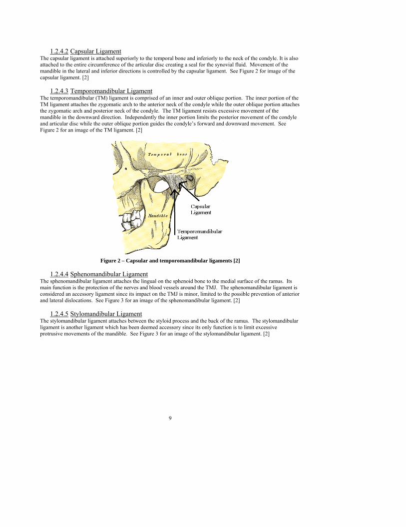
1.2.4.2 Capsular Ligament The capsular ligament is attached superiorly to the temporal bone and inferiorly to the neck of the condyle. It is also attached to the entire circumference of the articular disc creating a seal for the synovial fluid. Movement of the mandible in the lateral and inferior directions is controlled by the capsular ligament. See Figure 2 for image of the capsular ligament. [2]

1.2.4.3 Temporomandibular Ligament The temporomandibular (TM) ligament is comprised of an inner and outer oblique portion. The inner portion of the TM ligament attaches the zygomatic arch to the anterior neck of the condyle while the outer oblique portion attaches the zygomatic arch and posterior neck of the condyle. The TM ligament resists excessive movement of the mandible in the downward direction. Independently the inner portion limits the posterior movement of the condyle and articular disc while the outer oblique portion guides the condyle’s forward and downward movement. See Figure 2 for an image of the TM ligament. [2]

Figure 2 – Capsular and temporomandibular ligaments [2]

1.2.4.4 Sphenomandibular Ligament

The sphenomandibular ligament attaches the lingual on the sphenoid bone to the medial surface of the ramus. Its main function is the protection of the nerves and blood vessels around the TMJ. The sphenomandibular ligament is considered an accessory ligament since its impact on the TMJ is minor, limited to the possible prevention of anterior and lateral dislocations. See Figure 3 for an image of the sphenomandibular ligament. [2]

1.2.4.5 Stylomandibular Ligament The stylomandibular ligament attaches between the styloid process and the back of the ramus. The stylomandibular ligament is another ligament which has been deemed accessory since its only function is to limit excessive protrusive movements of the mandible. See Figure 3 for an image of the stylomandibular ligament. [2]

10

Figure 3 – Sphenomandibular and stylomandibular ligaments [2]

1.2.5 Temporomandibular Joint

1.2.5.1 Components and Functions The motion of the human jaw is made possible by the TMJ. It is composed of the temporal bones’ articulating surfaces (the mandible fossa and the articular tubercle), the upper portion of the mandible (the condyle), the articular cartilage and disc, ligaments (the temporomandibular and capsular), and muscles; as shown in Figure 4 [3]. The TMJ is a diarthrodial joint, or “movable joint”, because it allows relative movement between two bony surfaces separated by cartilage [4]. The system could be considered as two joints that work together to allow the motion of the jaw. The lower portion of the articular disc and the condyle allows the jaw to act as a hinge and rotate. The upper portion of the disc and the temporal bones articulating surfaces allow the jaw to slide forward and backward, and limitedly from side to side [2]. Functions of the disc include shock absorption, bone fit in the TMJ, facilitating complex movements, force distribution over a larger area, protecting the edges of the articulating surfaces, and spreading lubrication [5]. The articular disc is a complicated system. The thin disc that is considered to act as non-ossified (non-hardened) bone [3] sits below the mandible fossa and articular tubercle and above the condyle. When compressed it creates a concavo-convex shape on its upper surface and its concave lower surface facilitates the various motions of the jaw during each of its functions [2]. A loose fibrous structure connects the bone to the cartilage creating an articular capsule [6]. The disc itself is primarily a mesh of collagen fibers with interstices filled with proteoglycans. During loading the collagen maintains the disc’s shape. The elastin fibers assist in the recovery after unloading. Between the disc and the bones are synovial cavities which are lined with endothelial cells that create synovial fluid which lubricates the joint to reduce friction during motion [3].

11

Figure 4 – Sagittal view of the TMJ

The TMJ is not controlled by the neuromuscular system, rather it is controlled by existing biomechanical restraints. There is very little blood and few nerves in the disc itself [3]. Both Rees in 1954 and Isberg-Holm &Westesson in 1982 showed with cadavers that in the absence of the neuromuscular control system the disc and condyle behaved normally and suggested that biomechanical restraints dictated the movements of the TMJ. During jaw opening the condyle rotates approximately 10-15o on the disc. The taut temporomandibular ligament pulls the disc and condyle down the anterior of the articular eminence. The force from the elevator muscle pulls the condyle into the articular eminence compressing the disc creating an annulus to hold the condyle in place. The annulus is a bulging rim around the disc. The disc shape is not genetically predetermined and the size and shape of the annulus will change depending on the direction of the force. This can be seen in Figure 5. The amorphous disc actually destabilizes the condyle allowing its complex movements of sliding and rotating [5].

Figure 5 – TMJ in relaxed state (left); TMJ during clenching (right) [5]

1.2.5.2 Finite Element Analysis and Models

Progress has been made in understanding the forces withstood by the disc and other TMJ components. However, currently the most advanced finite element analysis (FEA) is done based on assumptions. The most detrimental assumption is that the disc acts with linear elastic properties, which is known not to be true. Other assumptions that have been made are that direct muscle contact and interaction with the disc is negligible even though the upper head of the lateral pterygoid muscle is attached to the disc and the condyle. Another assumption is that friction can be neglected due to an extremely small coefficient of friction. It has been found that during grinding, chewing of food,

12

or bruxism is when the condyle is subject to its greatest load “acting as a fulcrum” [5]. During grinding the jaw is balanced by the muscles and the condyle and disc are located on the posterior slope of the articular eminence. The condyle is kept in place by the annulus that is created when the disc is compressed. One FEA model that has been created to calculate the stresses in the articulating surfaces was done by Chen and Xu [7]. They created a 2-D model of the human TMJ using the assumptions discussed. The inputs for their model were the condylar displacements recorded with an MRI during jaw closing. A measured displacement that they used in their calculation was 0.61mm with a 1.3o counterclockwise rotation (d = -0.55i + 0.27j mm from the initial position). The model was used to simulate a jaw dropping to create a 9mm incisal opening. The disc experienced the greatest von Mises and compressive stress at 8.0 MPa. This occurred in the middle portion of the upper boundary of the disc. The articular eminence experienced the greatest tensile stress of 4.2 MPa [7]. See Table 1 for the stress results from this FEA. Table 1 - Finite element analysis TMJ stresses [7]

Max Von Mises Stress Max Compressive Stress Max Tensile Stress Articular Disc 8.0 MPa 8.0 MPa 3.7 MPa

Condyle 3.0 MPa 4.0 MPa 1.0 MPa Articular Eminence 3.9 MPa 2.8 MPa 4.2 MPa

A 3-D FE model of the TMJ was done by the Biomedical Engineering Department at the University of Iowa [21]. The 3-D model compared the motion of the articular disc and condyle when the disc was not loaded to the motion when the disc was additionally loaded with lateral and medial forces. The model was based on a 20 step static analysis of the normal opening of the jaw. It was found that muscle contractions and elastin fibers attached to the disc were not needed to create the motion observed. Although it was found that without these attachments the overall stress in the TMJ was greater. Figure 6 is a plot of the von Mises stresses during normal opening of the jaw. The springs represent attachments to the disc, which includes ligaments and elastin fibers. Figure 7 shows the differences in von Misses stresses when the anterior forces are applied.

13

Figure 6 – Von Mises stresses during normal opening of the jaw [8]

Figure 7 – Von Mises stress comparison with and without anterior force applied [8]

1.2.5.3 TMJ Failures and Disorders

TMJ disorders have been attributed to the disc sliding out from underneath the condyle. In these conditions the disc is malformed and it is not behaving as it should. When this happens patients have reported an audible click that occurs each time they open and close their jaw. With the disc out of place the condyle pushes up against it. As the disc wedges underneath, it builds up elastic potential energy. When this energy is released the disc slips back under the condyle; that is when the click occurs again [5]. This can be seen in Figure 8.

14

Figure 8 – Disc failure causing audible clicking [5]

1.2.6 Muscles In the human body there are three basic types of muscle: skeletal, smooth, and cardiac. These control everything from blood flow to digestion. The skeletal muscle is the most prominent muscle in the body. Its main function is to control the motion of bones. Smooth muscle makes up the digestive system, blood vessels, bladder, airways, and the uterus. This muscle is capable of staying contracted for long periods of time or stretching. The last type of muscle, known as the cardiac muscle, is found only in the heart. This muscle is very unique in that it has the ability to both stretch like smooth muscle and has the power to contract like a skeletal muscle with a higher endurance level then either of the others. The human jaw is controlled by skeletal muscles [9].

1.2.6.1 Skeletal Muscle Introduction Skeletal muscle is only capable of contraction, but this action is the sum of several complex processes. Sarcomeres are the contractile unit of muscles composed of myosin and actin fibers (See Figure 9) [10]. The basic motion of a muscle resembles the way a millipede uses its legs to walk. The fundamentals of both muscle contraction and millipede movement consist of two layers moving laterally in comparison to each other. For the millipede the two layers are the ground and its body. It stretches out its legs, grips the ground, and pulls its body forward. The protein fibers in muscle called myosin consist of many golf club shaped “legs”. These “legs” bond to the actin fibers (See Figure 9). The myosin is capable of producing a power stroke when attached to actin, pulling the layers laterally opposite of each other causing the contraction. This action happens repeatedly until the muscle is fully flexed [9].

15

Figure 9 – Muscle in relaxed (left) and flexed (right) state

1.2.6.2 Skeletal Muscle Motion

When someone decides to move a muscle the brain sends an electrical signal along a nerve to that muscle to tell it that it is time to perform. This signal travels all the way to the end of the nerve which terminates with a small gap between it and the muscle cell, called the synapse. The electrical signal jumps the gap and binds to a protein known as a receptor. The signal then travels along the cell until it enters the T-tubule. The T-tubule is the gateway for nerve signals to enter the cell. The signal then proceeds to tell the muscle to release its calcium stores. These stores are held in the area called the sarcoplasmic reticulum. Once the calcium leaves the sarcoplasmic reticulum it travels to the actin fibers in the muscle as can be seen in Figure 10. These fibers are shaped like a double pearl string spun in a helical pattern. The fibers are covered by a rod like layer known as tropomyosin along with troponin molecules as shown in Figure 9 and Figure 11 [10]. These two act together to prevent the myosin from connecting with the actin when the muscle is in its relaxed state. The calcium joins with the troponin to change the shape of the tropomyosin. The binding surfaces of the actin layer are exposed at this point for the finger-like myosin to connect to. The myosin contract, pulling the two layers laterally to each other. One stroke can shorten the muscle by 1%. Since a muscle can shorten 40 to 50%, this process must be repeated many times. For the myosin to release its bind from the actin, an adenosine triphosphate (ATP) must come and connect to the myosin as seen in Figure 9. Once this has occurred the ATP is broken down into adenosine diphosphate (ADP) and a phosphate group (Pi) causing the myosin return to its original position, ready for the action to begin again. When the muscle contraction is complete the calcium returns to the sarcoplasmic reticulum and the muscle relaxes [9].

16

Figure 10 – Nerve ending and T-tubule

Figure 11 – Skeletal muscle breakdown

17

1.2.6.3 Skeletal Muscle in the Jaw Since the jaw is capable of motion on all three axes, there are several muscles in place to facilitate the movement. The sides of the jaw are mirrors of one another. In order to focus on the opening and closing of the jaw there are seven main muscles. The temporal, masseter, medial pterygoid, and lateral pterygoid muscles are the main muscles for closing or elevating the jaw. The digastric, suprahyoid, and infrahyoid muscles are depressor muscles involved in jaw opening. There are also ligaments that effect the opening and closing motions; the collateral discal, the capsular, and the temporomandibular ligament [3]. The depressor muscles attach the mastoid process to the mandible and the hyoid. The digastric muscle connects the mastoid process to the mandible and is connected to the hyoid by a tendon. The suprahyoid muscles are connected from the mandible to the hyoid, and the infrahyoid muscles are connected from the hyoid to the sternum and clavicle. The depressor muscles work to open the jaw and also in swallowing. The digastic muscle works mainly when quick opening is required and when the mandible is opened against resistance [11]. The muscle and bone structures are shown below in Figure 12 and Figure 13 [2]. As a group the main forces to overcome are that of the elevator muscles and ligaments in order to open the jaw [12]. The ligaments act as springs, with no resistance when in compression and a spring stiffness value of 10.9-16.35 kN/m when in tension [3].

Figure 12 - Depressor muscles

Figure 13 - Hyoid bone and mastoid process

18

The elevator muscles are somewhat more complex because they also function in positioning the jaw. The temporal muscle is a large fan shaped muscle attached to the temporal bone, which comes together through the zygomatic arch and attaches to the coronoid process of the mandible. The temporal muscle is often explained as having three distinct parts: anterior, middle, and posterior. The temporal muscle acts as an elevator and positioner. As an elevator it is used more for speed and not to resist high forces. The three sections of the temporal muscle can activate separately allowing it to work as a positioner. The vector force that the temporal muscle exerts on the jaw line can be seen below in Figure 14 [11].

Figure 14 - Temporal muscle vector force [11] and muscle [2]

The masseter muscle generates the high forces that the temporal muscle does not. It connects the angle of the mandible to the zygomatic arch. It can generate very high loads in the molar area, and is the most powerful muscle of the mandible. The vector forces can be seen in Figure 15. [11]

Figure 15 - Masseter muscle vector force and muscle

The medial pterygoid muscle works with the masseter muscle. It is connected to the internal section of the mandibular angle and to the pterygoid plate which is internally part of the mouth. The pterygoid plate can be seen in Figure 16. The medial pterygoid can exert high forces, but not quite as large as the masseter. Though the medial muscle can act as a positioning muscle this is not its main function. It acts to move the jaw in closing as well as lateral, or side to side, motion. The medial muscle acts upward, forward and inward on the mandibular angle, and can be seen in Figure 17. [11]

19

Figure 16 - Sphenoid bone including the pterygoid plate [2]

Figure 17 - Medial and lateral pterygoid muscles in skull [2] and medial pterygoid muscle[11]

The muscles of the masseter and medial pterygoid are braided in order to increase the strength of the muscle. The muscle fibers are at an angle, an arrangement typical of strong muscles, unlike the parallel arrangement of the temporal muscle. A view of the vector forces caused by these muscles can be seen in Figure 18. [11]

20

Figure 18 - Vector forces from masseter and medial pterygoid muscles [11]

The lateral pterygoid muscle is actually two muscles, superior (upper) and inferior (lower). The upper lateral pterygoid muscle connects to the sphenoid bone, to the condylar neck, capsular ligament, and the articular disc. The lower lateral pterygoid muscle connects from the pterygoid plate to the condylar neck as seen in Figure 19. The two muscles must work in unison moving both the disc and the condylar neck in opening the jaw or else the jaw may ‘click’. They work to create lateral and protrusive movement of the mandible. The upper lateral muscle affects upward, forward, and medial forces on the condyle and disc. This is used for positioning and to ensure the disc remains between the condylar and eminence. The upper moves the disc down and forward and the lower moves the condyle down and forward.[11]

Figure 19 – Lateral pterygoid muscle[11] and condylar neck[2]

The teeth and the condylar process create reactive forces against the closing of the jaw. The ligaments and elevator muscles create reactive forces against the depressor muscles. The total forces can be seen in 1-D and 3-D in Figure 20.[11]

21

Figure 20 - Summarized 3-D vector forces on the jaw[11]

In order to focus on opening and closing the jaw, assumptions must be made. Lateral motion of the jaw will be ignored for the time being. Opening and closing of the jaw are not the reverse of each other. According to Koolstra (1997), in opening the jaw slides forward while rotating and then continues to rotate to complete opening, regardless of the different levels of muscle activation. Different degrees of opening result in different steps of sliding and rotating. The sliding varies somewhat with different levels of muscle activation. The motions of 100% activation can be seen in Figure 21; the different outlines indicate the position of the jaw at sequential steps of time. In opening the jaw the inferior lateral pterygoid is important in causing the sliding motion. In Koolstra’s study, the researchers deactivated different muscles, and the inferior lateral pterygoid created the biggest difference in sliding. When the digastric was deactivated, the jaw slid, but did not open as wide as the others. In order to fully simulate opening motions, five muscles per side of the jaw would need to be modeled: three depressor muscles, the temporal, and the lateral pterygoid muscle. The temporal and lateral pterygoid muscles can be further broken down into three and two components respectively for even further accuracy. [12]

22

Figure 21 - Jaw opening at 100% muscle activation [12]

The closing motions of the jaw can be seen below in Figure 22 at 5% of the total muscle force. The muscles of closing can produce much higher forces than are needed just for closing in order to chew and clench. Therefore, a small percentage of the muscle force can be used to completely close the jaw. According to Koolstra (2001 and 1997), the passive muscles of the jaw closing limit the amount of jaw opening. The jaw closing was not very affected by the passive depressor muscles. The TMJ was loaded in both opening and closing. The moments as well as the forces of the elevator muscles are essential for stable operation of the TMJ. They found that movements of the jaw were predominantly dependant upon the orientation of the contributing muscles and not on the TMJ ligaments or passive muscle forces. The muscles needed to simulate jaw closing are the temporal, masseter, lateral pterygoid, and medial pterygoid muscles. In Koolstra’s study removing certain muscles from the simulation, only removing the temporal muscle resulted in incomplete closing. [12][13]

Figure 22 - Jaw closing at 5% muscle activation [12]

Deformations of the mandible will be important when considering chewing, however since the goal of this stage of the project is to model closing of the jaw, deformations should not impact our design.

23

According to Koolstra (2002), the maximum jaw opening that can be achieved in simulations is usually around 3 cm. However, in reality the jaw can open closer to 6 cm. [14] Table 2, converted from Koolstra 2005, shows muscle lengths and maximum forces determined in their experiments.[6] The choice of muscles to be used in this project is explained in Chapter 2. Table 2 - Properties of muscles in simulation [6] Muscles Muscle length (mm) Max. force (N) Superficial masseter 48.0 272.8 Deep anterior masseter 29.5 73.8 Deep posterior masseter 30.9 65.8 Anterior temporalis 57.4 308.0 Posterior temporalis 62.9 222.0 Medial pterygoid 43.3 240.0 Superior lateral pterygoid 29.1 38.0 Inferior lateral pterygoid 27.2 112.8 Anterior digastric 51.9 46.4 Geniohyoid 48.5 38.8 Anterior mylohyoid 21.8 63.6 Posterior mylohyoid 44.8 21.2

1.3 Mechanical Simulations of the TMC 1.3.1 Muscles Simulating a human muscle is a very complicated endeavor. Although mimicking a muscle’s strength, speed, or size is easy, accomplishing all of these capabilities with one man-made device is extremely difficult. Currently there are several options on the market used in simulations. These include, but are not limited to, hydraulic and pneumatic rams, servo drives, air muscles, electroactive polymers, and muscle wire. Each option has its own pros and cons and these must be weighed in accordance to the user’s requirements.

1.3.1.1 Requirements To accurately reproduce the movements of the human jaw all of the characteristics of each muscle need to be as near as possible to real life. The ability to apply relatively large forces, close with great speed, or match the same exact size are not necessary, however, the basic principles must remain similar.

1.3.1.2 Hydraulic and Pneumatic Rams Hydraulic and pneumatic are the most widely used types of piston ram. Rams use the pressure of their transmitting fluid to create a force. A pump compresses the fluid into one side of the ram which forces the piston to move in the opposite direction (See Figure 23). Hydraulics use oil as their transmitting fluid and pneumatics use air. Hydraulics are capable of creating extreme forces that are usually only limited by the pump. This same principle holds true for the speed of the ram. The higher the flow rate of the pump, the faster it transfers fluid into the ram, thus moving the piston at greater speed. Pneumatics are capable of great forces as well but are used less frequently then hydraulics for heavy lifting. Pneumatics are more often used for their high speed capabilities. One of the downfalls to rams is the extra equipment and plumbing. Hydraulics can become messy due to all the oils involved and this is a great drawback when working with highly sensitive electronics. There is also the large installation area needed for these types of units. To achieve certain forces specific pump and ram size are necessary, that is, as the required level of force increases so does the size of the equipment [15].

24

Figure 23 - Hydraulic ram

1.3.1.3 Servo Drives Servo drives are position controlled electric motors. They are used frequently in such devices as hobby vehicles and in robotics as seen in Figure 24. They are capable of extremely high speeds, but lack the power that a ram has. Most servos consist of a small electric motor enclosed in a housing with a position sensor (typically a potentiometer) and various other electronic controls. The motor shaft is then connected to a push rod that moves the desired load. This means the force of the servo is greatly hindered by the length of the lever arm that works against the motor. To their advantage, servos can have a great deal of precision depending on their internal gearing. This can be used to produce easily repeatable results during testing [15].

Figure 24 – Servo drives in spider robot

1.3.1.4 Air Muscles

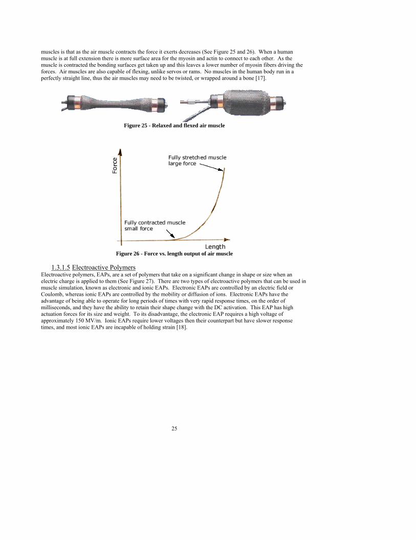
Air muscles are based on the same principle as hydraulics and pneumatics. Air is forced into a balloon like tube causing it to expand horizontally but contract laterally. The motion looks very similar to flexing the bicep muscle. The balloon starts out long and thin but as air is pumped into it the balloon begins to take on a circular shape. This causes the two ends to contract towards each other. This device is capable of high forces compared to its size and weight. Again, the speed is limited by the pump that is used to transmit the air. Another key similarity to human

25

muscles is that as the air muscle contracts the force it exerts decreases (See Figure 25 and 26). When a human muscle is at full extension there is more surface area for the myosin and actin to connect to each other. As the muscle is contracted the bonding surfaces get taken up and this leaves a lower number of myosin fibers driving the forces. Air muscles are also capable of flexing, unlike servos or rams. No muscles in the human body run in a perfectly straight line, thus the air muscles may need to be twisted, or wrapped around a bone [17].

Figure 25 - Relaxed and flexed air muscle

Figure 26 - Force vs. length output of air muscle

1.3.1.5 Electroactive Polymers

Electroactive polymers, EAPs, are a set of polymers that take on a significant change in shape or size when an electric charge is applied to them (See Figure 27). There are two types of electroactive polymers that can be used in muscle simulation, known as electronic and ionic EAPs. Electronic EAPs are controlled by an electric field or Coulomb, whereas ionic EAPs are controlled by the mobility or diffusion of ions. Electronic EAPs have the advantage of being able to operate for long periods of times with very rapid response times, on the order of milliseconds, and they have the ability to retain their shape change with the DC activation. This EAP has high actuation forces for its size and weight. To its disadvantage, the electronic EAP requires a high voltage of approximately 150 MV/m. Ionic EAPs require lower voltages then their counterpart but have slower response times, and most ionic EAPs are incapable of holding strain [18].

26

Figure 27 - EAP claw

1.3.1.6 Muscle Wire Muscle wire is a type of shape memory alloy made of Titanium Nickel (TiNi) and is known in the industry as either Nitirol or Flexinol. Muscle wire is pictured in Figure 28. This alloy is called a memory alloy because it can be programmed with two specific lengths. The length change is based on the temperature of the material. At the cooled temperature (dependent on the specific alloy) the spring like material is flexible and stretchy, while at the heated temperature (also dependent on the specific alloy) the material contracts and becomes stiff. These artificial muscles have extremely high power-to-weight ratios but are very light-weight so their actual power output is weak. They are easily susceptible to damage when in the cool state. Like a spring, an overstretched wire will not go back to its original form [19].

Figure 28 - Muscle wire arm

27

1.3.2 Ligaments At the forefront of artificial ligaments is tissue engineering technology. Tissue engineering is the development of synthetic materials that can be used to replace damaged tissues in the body. The materials can also be put to use in a model of the human jaw. Several materials have already been developed and tested for use, including Gore-Tex, Dacron, Carbon Fiber, and LAD. Each of these materials is defined by their base material and the method used in creating each fiber, from braids to several interwoven loops. A breakdown of the advantages and disadvantages of each material and some material properties of each can be found in Table 3. Unfortunately these materials may not be adequate for application in our model because they do not share similar material properties. One such property is the stiffness of the ligaments. The TMJ ligaments have a stiffness of around 10.9-16.35 kN/m [3]. In addition, the TMJ is a more complex ligament because of its wide range of movements that must have some slack to allow motion. More research is needed on the material properties and forces affecting the ligaments before a suitable material for the artificial ligaments can be determined. [20] Table 3 - Commonly used synthetic ligaments. [21]

Advantages Disadvantages Ultimate Tensile

Strength (N) Stiffness (N/mm)

Elongation at break (%)

Gore-Tex

High strength and fatigue life, limited particle debris

Lack of tissue ingrowth, fraying at bone tunnels, chronic effusions, ultimate longevity

5300 322 9

Dacron

High Strength, supported collagenous ingrowth

Stress-shielding of collagenous ingrowth, rupture of the femoral or tibial insertion, rupture of central body, elongation

3631 420 18.7

Carbon fiber Synthetic material

Particulate matter, foreign body response in synovium

660 230 x 109 1

LAD Protects graft during maturation

Inflammatory reaction, high complication rate

1730 56 22

1.3.3 Articulating Disc Simulating this complex joint would be useful for various reasons from research to prosthetics. The non-linear elastic properties make material selection extremely difficult. Crude computer models give an idea as to where to start. According to Fontenot’s experiments in 1985, the elastic modulus of the disc can be estimated at 1.8 MPa [7]. With this in mind a material could be selected that would be used to create an artificial disc. Ideally one material could be found that had the elastic properties capable of deforming and reforming as needed by the disc. If a fluid material was used, a casing material could be used to create a type of pouch. A thermoplastic elastomer with an elastic modulus equivalent to that found by Fontenot could be used as a disc. However, with both of these suggestions comes the problem of friction. In the TMJ the friction is almost zero and is generally neglected. Lubrication would be necessary for any design using a rubbery polymer or pouch. A low friction, no lubrication design could include a delrin or nylon disc. The drawbacks to this would be that it would not deform as necessary for the full range of jaw motions. This could be used as a temporary measure to get started by making a disc that would facilitate only opening and closing or clenching. 1.4 Products and Patents While there are many patents relating to the human jaw, there are few that apply to human jaw motion simulators and the disc in the TMJ. Of the products and/or patents that were found, only manual and virtual models are available for creating a human jaw. Few, if any, mechanical models exist because of the lack of knowledge of how the muscles and ligaments in the jaw work, therefore there is no solid way to recreate them mechanically.

28

1.4.1 Implant Rosenbaum et al. have created a TMJ disc implant; it is comprised of a robust material that has a filling solution or is made of an open cell fibrous material with a solution inside. It is to be surgically implanted into the TMJ. The outer material is biocompatible so that the body does not reject it once implanted[22]. The abstracts for different patents researched can be seen in Appendix A . 1.4.2 Manual Applications Manual applications are most commonly used by dentists to check the contact points of teeth in a patients jaw. Usually, they consist of a top dental arch and a bottom arch that are hinged or attached to a number of things, such as sticks, pins or movable platforms to name a few (see Figure 29). Generally called dental articulators, they let the dentist move the top and bottom part of the jaws so that when they create new dental fixtures, such as new teeth or dentures for a patient’s mouth, the new item will fit with the already existing teeth and bite. They allow for the three movements of a jaw: opening and closing, lateral shift, and retrusion and protrusion. Because there are no mechanical parts to move the articulator, it is moved manually by the doctor and can therefore cover any range of movements. As with a real human jaw, the bottom arch is usually the item that moves while the top one is fixed to remain stationary.

Figure 29 - Common dental articulator [23]

1.4.3 Virtual Applications Possibly the most common type of human jaw motion simulation are the virtual models. Perhaps these are the most widely developed because so little is known of how the muscles and ligaments in the jaw actually work that virtually simulating the jaw will allow for further study into what muscles are used during jaw motions. There are a few different types of virtual models, the prominent one being the orthodontic models which are used much like dental articulators. They can be obtained by scanning a patient’s jaw and teeth using various reference points to create a 3-D model on a computer. [24] “A Model to Simulate the Mastication Motion of the Temporomandibular Joint,” written by M. Villamil, describes how a group uses 3-D virtual modeling to further understand the TMJ. To create the virtual simulation, the group used a PQ5000 CT scanner to first obtain a jaw and skull to work from as shown in Figure 30. [25]

29

Figure 30 - CT scanning

The 3-D drawing that was obtained was then virtually cut into sections using a 3-D modeling program, as seen in Figure 31, to separate the mandible from the rest of the jaw so that it could later be manipulated. The different parts of the skull and jaw were then meshed (Figure 32) to create joined parts, separate from the mandible. The last step was applying forces to the TMJ so that opening and closing could be mimicked virtually. Equations and vector diagram for the forces can be seen in Figure 33.

Figure 31 - Separating the mandible

30

Figure 32 - Meshed sections

Figure 33 - Motion and forces of chewing [25]

A group of students from University of Maryland have also undertaken a virtual modeling of the jaw. They used Pro/Mechanica and 3D Studio Max for animating the jaw. In Pro/Mechanica, they used a lower jaw, a grinding block, and two teeth to animate the motion of the mandible (Figure 34). [26]

Figure 34 – Pro/Mechanica model

In 3D Studio Max, they first started with 2 blocks, the lower one pivoting like the lower jaw which can be seen in Figure 35. They furthered 3D Studio Max by importing jaw and tooth profiles from Pro/Engineer and were able to animate a few motions of the bottom jaw as shown in Figure 36.

31

Figure 35 – Beginning 3-D Studio Max animation of lower jaw [26]

Figure 36 – Final 3-D Studio Max animation of lower jaw [26]

In “Jaw Mechanism Modeling and Simulation”, the authors modeled the jaw virtually to analyze chewing through simulations; a sample of their force analysis can be seen in Figure 37. To control the motions, Matlab SimMechanics was used. [27]

Figure 37 - Model of jaw kinematics [27]

32

2 CHAPTER 2 – STAGE I: JAW CLOSING 2.1 Introduction 2.1.1 Problem Statement In order to thoroughly complete the project to include all motions of the jaw, it was necessary to break the project into stages. These stages are outlined below in Table 4. The goal for Stage I of the project is to achieve the motion of the human jaw closing. This must be done by controlling the muscle forces via a LabVIEW user interface. This must be accomplished in a way that would allow for further improvements and capabilities to be added to the system without a complete redesign or reconstruction. Table 4 - Stage outline

Stage Goal Stage I Jaw closing and initial set up Stage II Jaw opening and transition from opening to closing Stage III Jaw clenching and disc adaptation Stage IV Lateral jaw motion and chewing

2.1.2 Problem/ Design Concerns A complex force analysis must be done along with isolating the necessary components needed to accomplish the goal of simulating jaw closing.

2.2 Muscle and Ligament Use Decisions In order to complete the project within the given time frame and with a reasonable budget it was necessary to limit the scope of the first stage of the project. It was decided to limit the number of muscles simulated for jaw closing to three. The three main muscles for closing are the temporal muscle, the masseter, and the lateral pterygoid muscles. The temporal and lateral pterygoid muscles are important for positioning the jaw and disc during closing. The masseter muscle produces the main forces for closing. Although most researchers divide the temporal muscle into two or three sections, in order to limit the number of muscles, just one vector to simulate the temporal muscle will be used. The masseter muscle is sometimes broken down into components; again, just one vector will be simulated. The medial pterygoid muscle acts in the same direction as the masseter muscle, but on the interior of the mouth. Since it does not apply as high forces and the direction of force is redundant it will not be used in this stage of the project. Table 5 shows the muscle force values obtained from Koolstra and how they will be represented in the project. Table 5 - Muscle force values [6]

Closing Muscles Max. force (N) New Max (N) Superficial masseter 272.8 Deep anterior masseter 73.8 Deep posterior masseter 65.8

Merge to One Masseter 412

Anterior temporalis 308.0 Posterior temporalis 222.0

Merge to One Temporal 530

Medial pterygoid 240.0 Eliminate Superior lateral pterygoid 38.0 Inferior lateral pterygoid 112.8

Merge to One Lateral Pterygoid 150.8

33

Ligaments are used to avoid overextension of the jaw, they are important in opening, side to side motion and containing the synovial fluid around the disc. Since the focus is on closing, and realistically duplicating the synovial cavities is not feasible at this time, it is not necessary to replicate the ligaments. 2.3 Skull Research For this simulation a highly detailed physical skull must be obtained. It is crucial that the articulating surfaces are accurate for proper motion of the jaw. Two main options are available for obtaining a skull. One is to buy a prefabricated medical model of a skull. While these are readily available, material properties are not. It would also be difficult to create points for the muscles to attach to, and to mount the skull. The second option is to obtain a computerized model of a skull. This would allow for changes to be made for mounting and muscle attachment purposes, as well as to thoroughly map out the articulating surface to create a movement profile. While creating a physical prototype from a computerized model can be highly involved, the benefits of being able to adjust the model and map out the surfaces makes this option desirable. Mimics, software used to convert CT Scan files to 3-D models, and a CT scan file of a complete human skull were obtained from Materialise. Using the Mimics software the skull was edited to separate the mandible from maxilla, as well as to remove features created by noise. Since the human body is not perfectly symmetrical, it was decided to cut the skull down the center, so that one side could be thoroughly modeled and then mirrored to create a proportioned skull. Figure 38 shows an image of the mandible and maxilla created in the Mimics program.

Figure 38 – Maxilla and mandible created in Mimics

In order to create attachment points for the muscles, the anatomical origins and insertions were used. The origin of a muscle is the non-moving point of attachment; these are the anchor points on the maxilla in this case. The insertion of a muscle is the point of attachment that creates motion, which are the attachment points on the mandible. In a study by Koolstra in 1992, seven subjects underwent MRI to determine the insertion and origin points of six muscles on both the left and right sides. In this study, the temporal muscle measurements were taken as the anterior temporal and the posterior temporal, since this project is using only one vector for the temporal muscle, the average of the two was taken. The averaged results of the masseter, lateral pterygoid, and temporal muscles are shown below in Table 6 along with the actual values to be used in this project. The averaged values were compared to the modeled skull to get the actual attachment points to be used. The points are based on a zero point and axes shown in Figure 39. [37]

34

Table 6 – Muscle attachment values [37] Muscle Averaged Project Actual X (m) Y (m) X (m) Y (m)

Masseter Insertion 0.0185 -0.0643 0.0204 -0.0605 Origin 0.0338 0.0093 0.0338 0.0043

Lateral Pterygoid Insertion -0.0013 -0.0025 0.0032 -0.0044 Origin 0.0275 0.0071 0.0239 0.0064

Temporal Insertion 0.0365 -0.0180 0.0363 -0.0180 Origin 0.0166 0.0464 0.0167 0.0463

Figure 39 – Skull showing zero point and axes

2.4 TMJ Simulation Simulating the TMJ is a challenging task. This is because the TMJ is essentially frictionless. For this project there are three options to simulate the joint itself. The first option is to use a hard material with a low coefficient of friction, such as Delrin, to create a low friction surface and a high quality grease, such as Teflon, to further decrease the friction. The second option would be to use an elastic material, such as polyethylene foam, that would change its shape accordingly with the contour of the maxilla’s articulating surface. This option would also be used with a high quality grease that is compatible to use with the chosen material. The third option would be the similar to option one, using a hard material along with grease; however, the insert would be fixed to the mandible. This would be appropriate because of the assumptions made in the force analysis.

35

2.4.1 TMJ Friction Testing

Table 7 – Coefficients of Friction

Lubricated Surface A Surface B Coefficient of Friction

No Teflon Delrin 0.45No Teflon Teflon 0.5No Delrin Delrin 0.45Yes Teflon Delrin 0.08Yes Teflon Teflon 0.06Yes Delrin Delrin 0.1

Friction testing was done on a UniFlor grease, delrin and Teflon to determine which material or combination of materials would be best to coat the TMJ due to the exclusion of the TMJ disc, as seen in Table 7. During testing it was found that by just using the lubricant on any combination of materials greatly decreased the coefficient of friction in the joint. After receiving the polyurethane skull, more friction testing was done and it was concluded that by only using the grease in the joint, the coefficient of friction would be low enough for the project operating conditions and that there would be no need for coating the joint with additional materials. 2.5 System Control and Analysis To analyze the jaw closing motion, many factors had to be reviewed. The physical constraints and assumptions needed to be determined because the true motion of the jaw is not known. A method of controlling the motion also had to be established.

There are two ways to control the motion of the jaw system: force and position. Both control methods have their advantages and disadvantages. The attributes considered in the decision were, in order of importance, anatomical constraints, controllability, available knowledge, knowledge of control method, and physiological accuracy. Anatomical constraints are most important because the more constrained the system is the easier it is to control and to calculate the controls. Controllability refers to how capable the system is of being physically controlled via the chosen control method; in this case servo motors. Available knowledge is the amount of documented research done in the past from reliable sources. Control knowledge is the amount of knowledge readily available to the group. This is important because time constraints restrict further significant research. Lastly, physiological accuracy is important because a desired end result of this project is an understanding of the human jaw system. A more realistic system will provide a better understanding of the jaw. The decision matrix for system control can be found in Error! Reference source not found.. Table 9 - System control decision matrix

Anatomical Constraints Controllability

Available Knowledge

Control Knowledge

Physiologically Realistic

Value 5 4 3 2 1 Total

Force 1 2 1 1 2 20 Position 2 1 2 2 1 25

Muscle forces in the human jaw, as understood, are not a determinant system. A statically determinant system is defined by only three variables. Even with a simplified planar analysis of one side of the jaw, the system is statically indeterminate. From available knowledge the muscles are not anatomically constrained to impose specified forces. However, if proper assumptions are made, this system control method is more physiologically accurate because the muscles in the skull control force to move the jaw. Since the muscle forces should always be greater than or equal to zero it should be possible to control the force using tension alone. Unfortunately at the current moment the control of force using servo motors is not fully understood and a significant amount of time would have to be spent on more research.

36

Positionally the jaw is fully constrained. Disregarding TMJ disorders, the jaw moves in a defined path. Since this can be seen using multiple mediums (i.e. X-rays, MRIs, etc.) there is a large knowledge base available for use. Controlling position alone is not how the human jaw realistically functions. Also, controlling the position is not possible with a continuously positive tension or slack method as planned. Motors can unspool, but in this system a negative movement would require a compressive motion or rely solely on the other constrained points. Fortunately, positional control of motors is a well understood concept and would not require additional research. For this stage of the project, the system will be controlled positionally because the positional constraints are known and positional control method is well understood. Another benefit not weighed in the matrix is that with this method the forces on the simulated muscles can be monitored and captured as a data point to help better understand the human jaw. The results of the analysis done for the force method can be used as a check on the measured data from the positional method. 2.5.1 Positional Analysis In order to use position as a control at least two known points are necessary to place the jaw in 2D space. In this model there are a total of four constraints: three attachment points on the mandible and the single contact point with the maxilla’s articulating surface. All points are assumed to be in a single 2D plane. The three attachment points on the mandible are representative of the muscle attachments for the selected muscle groups: pterygoid, masseter, and temporal. In order to define the system, it has been assumed that the orientation of the mandible in the fully closed position (teeth touching) is always perpendicular to the slope of the articulating surface at the contact point on the tip of the condyle. To track the locations of the constraint points the model has been mapped out with a system of equations and calculated using a Matlab program which is included in Appenix B. The calculations can be found in Appendix C. The input constraints are the location of the contact point and the slope along the articulating surface at that point. The profile of the articulating surface was found using a cross section of the 3D CAD model of the skull as seen in Figure 40. A total of 560 points were mapped out on the profile of the surface. These points were used to calculate the slope at each of the 54 points that were chosen to be the steps of the closing simulation. The program outputs data into an Excel spreadsheet that has pre-formatted tables and plots to display information such as the path of travel of each attachment point (Figure 41) and the distance from the anchor to the attachment points at each step (Figure 42).

37

Figure 40 - Cross section of the TMJ with static analysis point locations

38

Figure 41. Path of Travel Plot

Figure 42. Muscle Lengths vs. Position Plot

39

2.5.2 Force Analysis To use force as a control for this system the positional constraints must still be calculated. Once the positional constraints were obtained the forces were calculated using a static analysis. The muscle forces controlled in this simulation are the temporal muscle (FT), masseter muscle (FM), and pterygoid muscle (FP). The free body diagram of the mandible is shown in Figure 43.

Figure 43 - Mandible free body diagram

By using three muscles and having the constraint of the maxilla’s articulating surface, the system is statically indeterminate due to there being four variables; FT, FM, FP, and FN (N for normal force). In order to fully define the system four non-redundant equations must be obtained. Since the system is being analyzed statically the force and moment balance equations were used for the first three equations. These can be found in Figure 43. To create the fourth needed equation the conservation of energy method was used. The theory behind this is that the change in potential energy of the mandible is equal to the sum of the work done by each muscle and the energy lost due to friction at the contact point of the articulating surface. This theory, however, has been abandoned due to it being redundant and resulting in a zero equals zero statement. A full explanation of equation variables and other force calculations can be found in Appendix C.

40

There were several design variables and assumptions that had to be defined to complete this analysis. The design variables include the attachment points of the muscles on the mandible and the muscle anchor points on the upper skull: To, Mo, Po, Ta, Ma, and Pa (T, M, and P for temporal, masseter, and pterygoid respectively). These points are based on anatomical research from Koolstra, 1992 as discussed in section 3.2.[37] The major assumptions made were that the mandible remains perpendicular to the slope of the articulating surface as discussed in section 3.1.1 and that the disc experiences a constant compressive force throughout the entire motion. The perpendicularity assumption allows for the disc to be left out of the model because its function of maintaining the orientation of the mandible is already accounted for. The normal force from the articulating surface, which directly correlates to the compressive force in the disc, has been assumed to be constant and to act at the contact point as discussed in section 3.1.1. Physical properties of the mandible such as the location of the centroid were found using ProE Mechanica. Mechanica was also used to find the mass and other properties that can be found in Appendix D. This information is necessary for an accurate force analysis of the system. The force analysis was completed using the same Matlab program as the positional analysis. At each of the points mapped out on the articulating surface the forces were calculated using the static equilibrium equations. The influential variables were the normal force and the coefficient of friction, which were chosen to be 15N and 0.1 respectively. The normal force was chosen to keep the loads on the system to a minimum; approximately at 10% maximum force capacity of the human jaw. The coefficient of friction was found through testing of various lubricants and skull material testing as discussed in section 2.6.1. The program outputs the theoretical values of the magnitude of the muscle forces as well as the vector components of the forces.

2.6 Muscle Simulation 2.6.1 Decision Matrix There are many complexities involved in simulating the muscles in the human jaw. Human muscle is an extremely sophisticated system that manmade objects have a hard time mimicking. While it is easy to simulate the size, speed, or power, it is not easy to achieve all muscles attributes in one unit. This makes it necessary to weigh the options to find the best overall solution for muscle simulation in a particular situation. This was accomplished through the use of a decision matrix as can be seen in Table 8. The options were laid out along the left side, and the requirements were placed along the top row. The requirements were weighted (1 to 5, 5 being the most important) to reflect their level of importance. Then each muscle option was given a rating of 1 to 10, 10 being the best, on how well it fit the requirement. Thus the option with the highest total is the best for this simulation. Table 8 – Muscle simulation decision matrix

Control Precision Accuracy Complexity Resources Safety Cost Total

5 4 3 3 3 2 2 High End Motor 161 10 10 10 3 6 6 1

Standard Motor 164 8 8 7 7 8 6 7

Pneumatic 78 4 3 4 3 3 3 5

Hydraulic 63 5 3 4 1 1 1 3

Air Muscle 68 4 2 3 2 3 3 5

41

Muscle Wire 118 3 6 5 8 6 5 6

Polymer 118 3 6 5 8 6 5 6

To properly simulate the motion of the human jaw, several key requirements stand out. Among the most important are control, accuracy and precision. Complexity, resources, safety and cost must also be considered. Control is the most important attribute in muscle simulation. Control is the capability to transfer exact speeds, forces, and distance requirements from an interface to the muscle simulator. Without this it will not matter how accurate or precise the simulation is because it will be impossible to tell it what to do correctly in a timely manner. This is why control received a weight of 5. Accuracy and precision are properties of the simulating device that defines how close it comes to a goal and how repeatable a certain outcome is. Precision was weighted higher then accuracy, with a 4 and a 3 respectively, because it was more important to have a repeatable simulation then an accurate one. If the force is five Newtons off every time this can be accounted for, however, if the force is only off a few Newtons unpredictably then there is error that cannot be tracked. The complexity, resource availability, and cost are also important considerations. A project may be limited to a certain scope that must be followed. There are also time constraints and budgets that limit a project. The amount of resources already available makes it easier to achieve goals on time and within budget thus scoring it a 3 along with complexity. The less specialized and sophisticated it is increases chances of having those resources accessible. Cost on the other hand can be slightly more flexible giving it a weight of 2, because it can be easier to justify a reason to apply more money to the project but it is impossible to change the time frame. Safety must always be considered including safety of the group doing the construction, the operator, and bystanders. Some muscle simulation devices such as hydraulics are more dangerous then others, but overall none of the options are truly life threatening and do not pose a health risk. There are minor concerns of burns, scrapes, and low level shocks. In general, hydraulics’ are the most dangerous but with the low forces required, there would not be high hydraulic fluid pressures. Safety was given a weight of 2 because of this. Based on earlier research (see section 1.2.6), each of the simulation options was given a rating reflecting how well it fulfilled each requirement. Standard precision motors showed to be the best choice. Even though they were never the best in any category, they consistently scored well in all categories. 2.7 Electric Motors There are a vast variety of motors available on the market that could be suitable for muscle simulation. It was again necessary to choose which would be best for achieving the goals of the project. While there are a huge number of options available there were only a few motor types that would work best for this type of muscle simulation. DC servo motors (brushed and brushless), stepper motors, shunt, and serial motors were all considered. 2.7.1 Motor Basics Motors work on the basis of magnetism. They are built with permanent magnets and coil windings (electromagnets). These permanent magnets and electromagnets use repelling and attracting magnetic fields to turn the output shaft of the motor. Basic motor construction consists of an outer housing, coil windings, a permanent magnet, and an output shaft that rides on a series of bearings located in the housing. Internally the motors use either a fixed magnet and a rotating coil, or vice versa. The stationary part is called the stator and the rotating part, the rotor [28]. Figure 44 shows a dismantled motor with its individual parts labeled. The way each is built and how power is applied is what determines its functionality. A few examples of this functionality are its ability to be accurate, precise, fast, and powerful.

42

Figure 44 – The internal construction of a standard electric motor [29]

2.7.2 Stepper Motors Just as the name implies, stepper motors are a style of motor that rotates in steps. The number of steps in a rotation is determined by the construction of the motor and can vary from low numbers in the double digits up to thousands. The outer electromagnet is constructed of a set of windings around a circle with teeth as shown in Figure 45. The number of teeth is representative of the number of poles and thus the steps. Circuitry is used to send a signal to the motor that makes it move one step at a time. The frequency of the input signals determines the speed, and the number of signals sent determines how many steps it rotates. This ability to have a discrete number of steps gives a stepper motor high precision. It can be rotated to a required angle and then brought back to that same angle repeatedly [30].

Figure 45 – A sample coil and magnet setup for a stepper motor [31]

2.7.3 DC Servo Motors There are two basic types of DC servo motors, brushed and brushless as seen in Figure 46. These motors are very similar in construction to the stepper motors but do not operate in the same manner. Unlike stepper motors, servo motors are not controlled by turning in steps. They instead use a constant winding and a permanent magnet. Brushed motors have the permanent magnet located on the stator and the coil windings are located on the rotor. A commutator and brushes are used to supply switching power to the rotor. In the brushless motors the magnet is

43

located on the rotor and the coils are the stator. A semiconductor is used in place of brushes for switching power in the coils. The elimination of the brushes benefits the motor. Without brushes to wear out, the brushless motors have much lower maintenance needs and the lack of brush debris in the motor provides better operation. Since the magnet is lighter than the windings, the brushless motors also have a lower inertia and better heat dissipation due to the windings being closer to the outer surface of the housing. The brushed motors are limited in peak power because the brushes put a mechanical limitation on power transfer due to sparking. Servo motors work on a closed feedback loop. This means they send signals back to the driver to confirm voltages and current where as stepper motors do not [32].

Figure 46 – The brushes of the brushed motor (left), as pointed out by the red arrow, provide power to the

coil. The brushless motor (right) has a stationary coil that is directly wired shown by the blue arrow. 2.7.4 Shunt and Series Motors Shunt and series motors have a different style of construction from steppers or servos. They use two coil windings instead of a coil and a permanent magnet. Series motors have the coils wired in series and the shunt motors are wired in parallel. This creates the differences in characteristics. The shunt motors are constructed of a thinner wire with more turns limiting them to lower torque levels at startup, making it useful only in situations when there is a lower initial shaft load. Series motors are capable of higher starting torque, but with series motors their speed is dictated by that torque. The higher the load on the shaft the lower the motors speed, thus with a low shaft load the motor has a higher speed. Shunt motors are capable of speed control by variations in current making them more controllable and thus more desirable in certain situations [33]. 2.7.5 Motor Choice To chose the best motor for this particular application the help from an expert in the field was enlisted. Professor Rifat Sipahi, Ph.D. teaches System Analysis and Control at Northeastern University, and received his Ph. D. at the Advance Laboratory of Automation Robotics and Manufacturing, in the Mechanical Engineering Department at the University of Connecticut [34]. He is very knowledgeable in the field of robotics and controls, allowing him to give helpful insight in the decision making process. Through research and advice it was decided that due to the ease of control, the functionality, and the accuracy and precision that brushless DC servo motors would be the best choice. Servo motors cannot be controlled by position without an additional device. A feedback loop is required to make a servo motor arrive at a certain angle. To create this feedback loop a rotary position sensor is needed. As the motor is rotated it sends positional information back to the controller so it can be tracked at all times. This allows the controller to stop power at the right moment so the motor arrives at the required angle. This adds to the cost and complexity of the motor and control system but is necessary for positional control. The torque of the servo motor is not proportional to speed, but rather load. Therefore the system is capable of measuring the force needed to move the jaw. Rotary position sensors (RPS) work with shaft rotation to create a proportional electrical output. RPS utilizes several different types of technology to create this signal. This includes, but is not limited to, resistance, capacitance, magnetism, and optics [38]. An RPS can be either installed on the output shaft of the motor or it can be

44

built in as seen in Figure 47. The sensor is used to create a feedback loop in the motor control setup. The sensor sends the electrical output to the controller. The controller then takes this signal and based on its programming executes new commands to the motor. For the jaw simulation the controller will cease power when the motor has arrived at the correct position.

Figure 47 – Built in encoders are part of the motor (left [39]) while others are added (right [40]) 2.7.6 Controlling A Motor In order to run any motor there are some required parts such as an interface, controller, driver, and necessary circuitry. LabVIEW was already chosen as the interface because of its user friendly characteristics. A NI PCI-7344 four axis servo/step motion controller is needed to connect to the computer. This part connects to a standard PCI slot of a desktop computer. The controller is four axis compared to the three axis needed for the motors because it is a standard model. When LabVIEW is installed on the computer it can communicate to this card which will then communicate to the driver. A SHC68-C68-S 68 pin VHDCI to 68 pin VHDCI cable goes from the PCI card to the driver. This is a specially designed cable suited for this purpose and is two meters long to allow space between the computer and the driver. A MID-2100 integrated three axis servo drive with power supply will take the signals from the PCI card and translate them to the motor. The driver was custom made for the three axis design. This driver has a built in power supply that will provide the power to the motors. From the driver, specific cables are needed to hook up different brand motors. Once this connection is complete a user is capable of setting up a LabVIEW program to control all functions of a DC servo motors operation [35]. The quote for these particular products can be seen in Appendix D.

45

3 CHAPTER 3 – DETAILED DESIGN 3.1 Digital Simulation The digital simulation was created using a Matlab graphical user interface (GUI). The GUI, as seen in Figure 48, obtains data from the output of the analysis program and displays critical information, such as a positional plot, muscle lengths, and theoretical force values. The GUI is fully controllable via open, close, step open, and step close buttons. The step buttons allow the user to open or close the virtual jaw in steps, whereas the open and close buttons themselves will begin to their cycle from current step. The force values at the position will be marked on the muscle force plot and the muscle lengths plot gives a visual representation of the three muscles in relation to one another. These can bee seen in Figure 48 and in a greater detail in Appendix F.

Figure 48 – Digital Simulation Interface

3.2 Design The detailed design consists of the closing motion being simulated using only three muscles on each side of the skull. Only three motors will be used to control this system, with each motor controlling its specific muscle on both sides of the skull. There are very low force levels therefore the design was construct of light weight material. Knowing that the design will be expanded upon in further stages, versatility is important. The design is a frame which holds the motors, pulleys, and skull as seen in Figure 49. Using a pulley system the motors connect to the skull to create motion. Each of these components is discussed in more detail in the following sections.

46

Figure 49 – Final Design

3.2.1 Frame The frame houses all three motors and the drive and reduction pulleys. It is made of 8020 extruded aluminum which has a t-slot on all four sides allowing objects to be mounted to it in a variety of positions. It is light yet strong and the adaptability made it a clear choice. 3.2.2 Motor and Controls Three motors are required to simulate six muscles. Since the jaw and its muscles are symmetric, one motor will be used to simulate the same muscle on both sides. A three axis controller, a three axis driver with power supply, and all the necessary wiring is also required as previously discussed in section 2.7.6. Information about the maximum forces of each muscle was determined through the research discussed in section 1.2.6.3. However, with an increase in the motor’s torque comes an increase in its price. Since each motor is actually doing the work of two muscles these torque levels can become very high and in turn so can the cost of the motors. The AKM33E Danaher Motion motor with 2.2 Nm torque and 680 rpm was chosen. This model was chosen because of the toque levels and that it has a built in encoder.

47

3.2.3 Pulleys For this project, it was decided to gear up the torque levels of the motors rather than purchase motors capable of producing the same force levels as the human jaw. This is to reduce money spent, weight, and the physical size of the motor tower structure. The idea was to use the motors like a winch to simulate the contraction of a muscle. This would keep true to our constraint that muscles can only apply force while contracting. A drive pulley is connected to the motor. This is then belted to a reduction pulley that drives an axle with each muscle group connected to it. This allows for simultaneous control of both sides of the jaw. This drive system can be seen in Figure 50.

Figure 50 – Motor and Pulley Connection

3.2.4 Wire Attachments and Guides Off the pulley axle, kevlar strings are attached with specially designed clamps that allow for slight tension adjustments. Since there are two strings attached to each axle this allows for precise balancing of the wires. From the clamp the strings travel down and pass over small screws located at the points where the muscles attach to the skull which is shown in Figure 51. The strings then travel down to the lower jaw where they are attached to another set of shoulder screws. The strings remain in one plane to eliminate any additional force vectors.

48

Figure 51 – Pulley to String Connection

3.2.5 Skull Each side of the skull has three attachment points and three anchor points, one of each for each muscle, to simulate the correct angles for the masseter, temporal, and pterygoid muscles. The wire is anchored to the attachment point and curves around the contact point, which is a small set screw. The back of the skull is flattened for mounting to the rest of the system. This is shown below in Figure 52.

49

Figure 52 – Skull with Anchor and Attachment Points

The skull design created in Mimics was created in 3-D using a Stereolithography Apparatus (SLA). This process takes a computerized image and converts it to a model by laser curing resin layer by layer. This produces an accurate model, however the material is brittle and directionally weak, because it was created in layers. The model was sent to US Surgical where a mold was created and several models were produced from the mold using polyurethane, this was accomplished using rubber molding. Based on the material properties of the polyurethane used, the diameters of the attachment and anchor points were created. The force applied to the attachment and anchor points creates a bending stress. Therefore the bending stress was calculated based on the maximum muscle force and compared to the yield stress of the material. Although studies show that for closing approximately 10% of total muscle force is required, the moments were analyzed for the total stress, to ensure they would be sufficient that maximum values. Bending stress is usually compared to 0.75 of the yield strength of a material. Polyurethane has different properties in flexing and tension. The flexural strength of 77.2 MPa (11,200 psi) was used for the yield strength. The bending stress was calculated as shown in appendix C along with the attachment diameters. The table below shows the diameters calculated. When these values were placed on the skull, the attachment point for the temporal muscle was large and would create conflict with the other muscles. Also, the diameter was larger than the area it was supposed to be located on. Since, it was designed to withhold maximum strength, but the system would likely only be applying 10% of this value, it was decided to reduce the outer diameter. 3.3 Motion Control To control the motors with LabVIEW, additional hardware was required as discussed in Section 2.7.6. A servo controller was purchased from National Instruments, which is a card that plugs directly into the computer and

50

interfaces with the LabVIEW program. The controller then is connected to a servo drive that takes the signals, converts them to work with the specific motors, and amplifies them to the right levels. Since this system has motors with encoders, positional information is fed back to the controller and therefore creates a highly precise and accurate system. 3.3.1 LabVIEW In order to create a LabVIEW program, a positional profile first had to be created in Microsoft Excel with the correct format. The x, y, and z positions were each a different column and each new 3 dimensional coordinate was placed in a different row. The positional profile was then used in National Instruments Motion Assistant program. Contouring parameters were set, such as the working space being 1-D, 2-D or 3-D, as well as if the program was to be written in counts per revolution or revolutions of each motor. The brushless servo motors used have a line count of 2048 and to determine the counts per revolution, also called quadrature counts, that number is multiplied by 4. The quadrature count for the motors used is 8192. Next, the contouring parameters must be set, which tells the motors how to move. The correctly formatted Excel file is loaded in and a motion profile is determined by the program. LabVIEW code is then generated through Motion Assistant as well as an SML file of the positional program. Once it is saved, it can be modified to have whatever outputs or feedbacks are needed for the specific use. For this project, a typical output would be the position of each motor over time. The LabVIEW program was also modified to ask the user to load an XML file at the start of the program. Appendix H includes a copy of the LabVIEW programming as well as all the settings required for Motion Assistant to create a LabVIEW code.

51

4 CHAPTER 4 – Results and Conclusions 4.1 Results The virtual simulation initially resulted in negative muscle forces and an unnatural movement, causing the jaw to open much wider than possible as shown in Figure 53. When this path of travel was used to create a control profile for the physical model it resulted in a critical failure. The connecting wires became slack and the mandible fell away from the maxilla.

Figure 53 – Virtual and Physical Failure

4.1.1 Physical Testing and Debugging In order to create a new position profile for the physical model, the mandible was held at different locations and the motors for the muscles were adjusted to hold it in place. Using this method a new set of data points were found and the motion program was run again. The physical closing motion of the jaw became more realistic as the jaw slid up the articulating surface and then rotated in the pocket. The motion was not inhibited by the lack of lubrication in the joint. 4.1.2 Virtual Testing and Debugging In order to correct for the failed motions a new path of travel was developed from the initial research on the system. As discussed in section 1.2.5.1 the jaw opens by first rotating 10-15° in the pocket of the joint before it slides down the articulating surface. This was adapted to create a new closing profile to make the lower jaw slide up the articulating surface and then rotate in the pocket to a complete close. The new profile was implemented in the virtual simulation with positive results. The path of travel now looks more realistic as shown in Figure 54.

52

Figure 54. Updated Path of Travel for Points on the Lower Jaw

4.2 Conclusion Based on the results of the virtual and physical simulations, it was determined that the condyle does not stay perpendicular to the articulating surface. From further testing, it was determined that the mandible’s motion is closer to a translation followed by rotation. However, this theory should be examined in future stages. The physical simulation showed that the coefficient of friction is so low in this stage of the project that there was no need for grease in the joint. However, in the future if a greater force is applied on the joint there may be a need for lubrication. 4.3 Future Progress To complete the jaw simulation, groups in the future stages should take the following steps. Further analysis needs to be done on the motion of the jaw and the movement of the muscles. A way to solve the indeterminate force analysis must be found. The LabVIEW programming will need to be updated to monitor torque values in order to calculate the forces of each muscle. The positional program and control of movement can also be improved to better match the realistic motion. A permanent absolute zero starting location, or a way to lock the motors, should be determined so that if the motors are moved when the system is off the program will always start at the same position. Muscle choices and simplifications will have to be expanded on in future stages in order to have better control over the closing motion of the jaw and to accommodate the other actions of the jaw. Ligaments and the TMJ disc should also be added for realistic jaw simulation.

53

5 CHAPTER 5 – REFERENCES 5.1 Sources Cited [1] Bioengineering Conference: A Ground-Breaking Forum for Surgeons and Bioengineers to Address Temporomandibular Joint Disorders, Broomfield, CO, May, 2005. [2] Gray, Henry, Anatomy of the Human Body, 20th ed. Philadelphia:Lea & Febiger, 1918. [3] Muftu, S., and Muftu, A., 2005, “Biomechanics of Tooth and Jaw”, Encyclopedia of Medical Devices and Instrumentation, pp. 1-58. [4] Brunksi, John B., “Tooth and Jaw, Biomechanics of”, Encyclopedia of Medical Devices and Instrumentation, Vol. 4 pp. 2776-2788. [5] Osborn, J.W. 1985, “The disc of human temporomandibular joint: design, function, and failure”, Journal of Oral Rehabilitation, Vol. 12, pp. 279-293. [6] Koolstra, J.H., and van Eijen, T.M.G.J., 2005, “Combined finite-element and rigid-body analysis of human jaw joint dynamics”, Journal of Biomechanics, Vol. 38, pp. 2431-2439. [7] J. Chen, U. Akyuz, L. Xu, R.M.V. Pidaparti, 1998, “Stress analysis of the human temporomandibular joint,” Medical Engineering & Physics, Vol. 20, pp. 565-572. [8] How Stuff Works, “How muscles work”, http://health.howstuffworks.com/muscle.htm, June 16, 2006. [9] Wikipedia, “Skeletal muscle”, http://en.wikipedia.org/wiki/Skeletal_muscle, June 16, 2006. [10]Caputo, Angelo A., Standlee, Jon P., Biomechanics in Clincal Dentistry, Chicago: Quintessence Publishing Co., 1987. [11]Koolstra, J.H., and van Eijen, T.M.G.J., 1997, “The Jaw Open-Close Movements Predicted by Biomechanical Modeling”, Journal of Biomechanics, Vol. 30, pp. 943-950. [12]Koolstra, J.H., and van Eijen, T.M.G.J., 2001, “A method to predict muscle control in kinematically and mechanically indeterminate human masticatory system”, Journal of Biomechanics, Vol. 34, pp. 1179-1188. [13]Koolstra, J.H, 2002, “Dynamics of the Human Masticatory System”, Critical Reviews in Oral Biology and Medicine, Vol. 13(4), pp. 366-376 [14] How Stuff Works, “How hydraulic machines work”, June 16, 2006; http://science.howstuffworks.com/hydraulic.htm,. [15] National Instruments, “Motor fundamentals”, June 16, 2006; http://zone.ni.com/devzone/conceptd.nsf/webmain/A18266D91803B4D18625685D006EC4E8 [16] Efunda, “Air muscle”, June 16, 2006; http://www.efunda.com/sponsors/inventables/airmuscle/airmuscle_intro.cfm?search_string=air%20muscle [17] The A to Z of Materials, “Electroactive polymers - EAPs”, June 16, 2006; http://www.azom.com/details.asp?ArticleID=885 [18] Wikipedia, “Muscle wire”, June 16, 2006; http://en.wikipedia.org/wiki/Muscle_wire [19] Baragar, F.A., and Osborn, J.W., 1984, “A Model Relating Patterns of Human Jaw Movement to Biomechanical Constraints”, Journal of Biomechanics, Vol. 17, pp 757-767. [20] Vunjak-Novakovic, G., Altman, G., Horan, R., and Kaplan, D.L., 2004, “Tissue Engineering of Ligaments”, Annual Review of Biomedical Engineering, pp. 131-156. [21] JW DeVocht, VK Goel, DL Zeitler, D Lew, and EA Hoffman, “Development of a Finite Element Model to Simulate and Study the Biomechanics of the Temporomandibular Joint”, Division of Physiologic Imaging, Dept. of Radiology, Univ. of Iowa; http://dpi.radiology.uiowa.edu/spie/paper10/VHPpaper.html [22] R. Rosenbaum, et al., "Temporomandibular joint disc implant", U. S. Patent 04,919,668, April 24, 1990. [23] S. Greene, "The Dental Articulator", June 16, 2006; http://www.qualitydentistry.com/dental/information/articulator.html [24] R. Sachdeva, "Method and apparatus for producing a three-dimensional model of an orthodontic patient", U. S. Patent 06,512,994, January 28, 2003. [25] M. Villamil, et al., “A Model to Simulate the Mastication Motion at the Temporomandibular Joint”, pp. 1-11, 2005; http://www.inf.ufrgs.br/cg/publications/mbvillamil/spie-2005.pdf [26] G. Alie, et al., “Animation of Human Manidular Motion”, April 14, 1999; http://www.glue.umd.edu/~zhang/414_99s/team/p1/

54

[27] B. Daumas, W. L. Xu, J. Bronlund, “Jaw Mechanism Modeling and Simulation”, pp. 1-8, 2005; http://www.massey.ac.nz/~wlxu/reports_pdf/mouth1.pdf [28] Electric Motors Reference Center, “Electric motors 101”, January 18, 2007; http://www.electricmotors.machinedesign.com/ [29] http://www.mae.ncsu.edu/courses/mae442/gould/AC_motor_picture.jpg [30] Advanced Micro Systems, “Stepper motor system basics”, January 18, 2007; http://www.ams2000.com/stepping101.html [31] Haydon Switch and Instrument, “stepper motor theory”, January 18, 2007; http://www.hsi-inc.com/stepper_motor_theory.php [32] Danaher Motion, “Brush vs. brushless”, January 14, 2007; http://www.danahermotion.com/education/learn_about_mc/servohandbook/motor/comparison/brush_vs_brushless.php [33] National Instruments, “DC shunt motors”, January 18, 2007; http://zone.ni.com/devzone/cda/ph/p/id/54 [34] Rifat Sipahi, Ph.D., “Bibliography”, January 18, 2007; http://www1.coe.neu.edu/~rifat/ [35] National Instruments, “Fundamentals of motion control”, January 18, 2007; http://zone.ni.com/devzone/cda/tut/p/id/3367 [36] MatWeb, “Material Property Data”, Dec 15, 2006; http://www.matweb.com [37] Koolstra, J.H., and van Eijen, T.M.G.J., 1992, “Applications and Validation of a Three-Dimensional Mathematical Model of the Human Masticatory System In Vivo”, Journal of Biomechanics, Vol. 25(2), pp.175-187. [38] Global Spec, “About rotary position sensors”, February 18, 2007; http://sensors-transducers.globalspec.com/LearnMore/Sensors_Transducers_Detectors/Rotary_Position_Sensing/Rotary_Position_Sensors [39] Thomasnet, “Step Motor/Driver offers optional built-in encoder”, http://news.thomasnet.com/fullstory/29947/1620 [40] Encoder Products Company, “Custom solutions”, February 18, 2007; www.encoderprod.com/customprod.html [41] Automation Solutions, “Technology in motion”, February 18, 2007; http://www.auto-sol.com/

Deleted: Haydon Switch and Instrument, “stepper motor theory”, January 18, 2007; http://www.hsi-inc.com/stepper_motor_theory.php¶[39]

Deleted: 40

Deleted: 41

Deleted: 42

55

APPENDIX A Patents

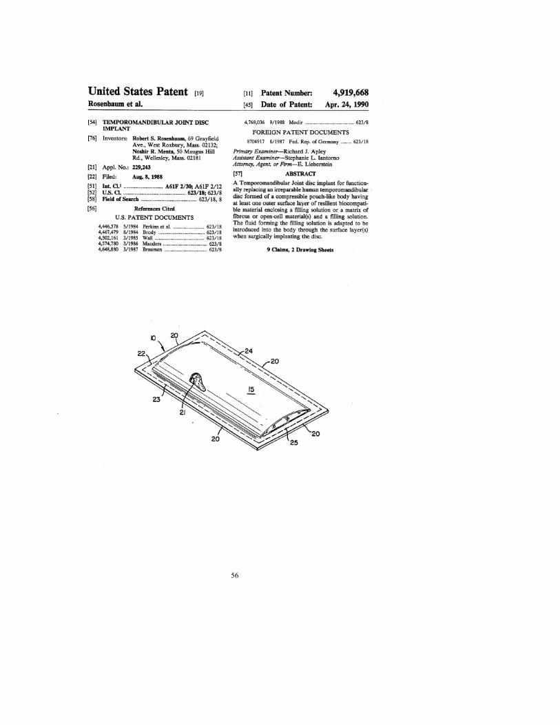
56

57

58

APPENDIX B

59

Matlab Code for Positional and Force Calculations and Interface %% Calculation Code %% Maloof 4-15-07 %% Positional and Force Calculation Program for Human Jaw %% This Program includes the most recent changes to the movement of the %% jaw, assuming that the jaw translates and then rotates %it also includes the old code that assumes both translation and rotation %% the origin is the contact point between the articulating surface of the %% maxilla and the disk/condyle %% program is written such that fumation of forces are all positive values %% (ie Fp + Ft + W = 0, W is negative due to internal equations) %% alpha is the slope at the contact point D = xlsread( 'ForcePositionDataReadFull.xls', 'Force & Position Data', 'B11:AH130'); DD = xlsread( 'ForcePositionDataReadFull.xls', 'Force & Position Data', 'C4:I5'); FN = xlsread( 'ForcePositionDataReadFull.xls', 'Force & Position Data', 'D7'); uf = xlsread( 'ForcePositionDataReadFull.xls', 'Force & Position Data', 'I7'); pin = xlsread( 'ForcePositionDataReadFull.xls', 'Force & Position Data', 'N7'); gears = xlsread( 'ForcePositionDataReadFull.xls', 'Force & Position Data', 'M3:M5'); for d = 15:83 %% R is the Rotational Matrix Based on slope of articulating surface alpha alpha = D(d,3); R = [ cos(alpha) -sin(alpha); sin(alpha) cos(alpha)]; %% (Global) Contact Point Nx = D(d,1); Ny = D(d,2); N = [Nx; Ny]; Nf = FN*[ sin(alpha); -cos(alpha)]; Nfx = Nf(1); Nfy = Nf(2); D(d,30) = Nfx; D(d,31) = Nfy; %% Kilograms, Based on ProE Mechanica Analysis mass = 0.100363; W = mass*(-9.8); %% P, M, T, C, Pa, Ma, and Ta represent the Pterygoid, Masseter, Temporal %% attachments on the Mandible, and their respective anchor points on the %% upper skull (on a single 2D plane). C (centroid) is determined by ProE %% Analysis of Mandible. %% Design Variables Based on Studies (2-14-07) %% Local muscle attachment point px = DD(1,2); mx = DD(1,4); tx = DD(1,6); cx = DD(1,7); py = DD(2,2); my = DD(2,4); ty = DD(2,6); cy = DD(2,7); %% need to check c values %% Global muscle anchor points Pax = DD(1,1); Max = DD(1,3); Tax = DD(1,5); Pay = DD(2,1); May = DD(2,3); Tay = DD(2,5);

60

%% Adding a conditional loop to make rotate 0-15 degrees and then translate if d > 67 %ROTATION & TRANSLATION %Defining points w/ equations p = [px; py]; %% Local Muscle Attachment Point (put in vector form) P = N + R*p; %% Global Muscle Attachment Point Px = P(1); Py = P(2); D(d,4) = Px; D(d,5) = Py; %% Input variables m = [mx; my]; t = [tx; ty]; M = N + R*m; T = N + R*t; Mx = M(1); My = M(2); Tx = T(1); Ty = T(2); D(d,12) = Mx; D(d,13) = My; D(d,20) = Tx; D(d,21) = Ty; c = [cx; cy]; C = N + R*c; Cx = C(1); Cy = C(2); D(d,28) = Cx; D(d,29) = Cy; else alphacc = -0.261799387799149; Rcc = [ cos(alphacc) -sin(alphacc); sin(alphacc) cos(alphacc)]; %NO ROTATION %Defining points w/ equations p = [px; py]; %% Local Muscle Attachment Point (put in vector form) P = N + Rcc*p; %% Global Muscle Attachment Point Px = P(1); Py = P(2); D(d,4) = Px; D(d,5) = Py; %% Input variables m = [mx; my]; t = [tx; ty]; M = N + Rcc*m; T = N + Rcc*t; Mx = M(1); My = M(2); Tx = T(1); Ty = T(2); D(d,12) = Mx; D(d,13) = My; D(d,20) = Tx; D(d,21) = Ty; c = [cx; cy]; C = N + Rcc*c; Cx = C(1); Cy = C(2); D(d,28) = Cx; D(d,29) = Cy; end %{ %% Defining points w/ equations p = [px; py]; %% Local Muscle Attachment Point (put in vector form) P = N + R*p; %% Global Muscle Attachment Point Px = P(1); Py = P(2); D(d,4) = Px; D(d,5) = Py; %% Input variables m = [mx; my]; t = [tx; ty];

61

M = N + R*m; T = N + R*t; Mx = M(1); My = M(2); Tx = T(1); Ty = T(2); D(d,12) = Mx; D(d,13) = My; D(d,20) = Tx; D(d,21) = Ty; c = [cx; cy]; C = N + R*c; Cx = C(1); Cy = C(2); D(d,28) = Cx; D(d,29) = Cy; %} %% Global Anchor Point in Vector Form Pa = [Pax; Pay]; Ma = [Max; May]; Ta = [Tax; Tay]; %% The following equations determine the force vector on the global system (ie Pr) %% This is used to find the unit vector (ie Pu) of the Force %% Vector from attachment point to anchor point (direction of force) Pr = Pa - P; Mr = Ma - M; Tr = Ta - T; Prx = Pr(1); Mrx = Mr(1); Trx = Tr(1); Pry = Pr(2); Mry = Mr(2); Try = Tr(2); Pux = Prx / sqrt( Prx^2 + Pry^2 ); Puy = Pry / sqrt( Prx^2 + Pry^2 ); Mux = Mrx / sqrt( Mrx^2 + Mry^2 ); Muy = Mry / sqrt( Mrx^2 + Mry^2 ); Tux = Trx / sqrt( Trx^2 + Try^2 ); Tuy = Try / sqrt( Trx^2 + Try^2 ); Pu = [ Pux; Puy]; Mu = [ Mux; Muy]; Tu = [ Tux; Tuy]; %% Unit Vectors Lp = sqrt( Prx^2 + Pry^2 ); %% Length from Anchor to Attachment Lm = sqrt( Mrx^2 + Mry^2 ); Lt = sqrt( Trx^2 + Try^2 ); %% Vector from attachment point to anchor point including pin radius (direction of force) Prp = pin*[ -Puy; Pux]; Mrp = pin*[ -Muy; Mux]; Trp = pin*[ -Tuy; Tux]; Prq = Prp + Pr; Mrq = Mrp + Mr; Trq = Trp + Tr; Prqx = Prq(1); Mrqx = Mrq(1); Trqx = Trq(1); Prqy = Prq(2); Mrqy = Mrq(2); Trqy = Trq(2); Pqux = Prqx / sqrt( Prqx^2 + Prqy^2 ); Pquy = Prqy / sqrt( Prqx^2 + Prqy^2 ); Mqux = Mrqx / sqrt( Mrqx^2 + Mrqy^2 ); Mquy = Mrqy / sqrt( Mrqx^2 + Mrqy^2 ); Tqux = Trqx / sqrt( Trqx^2 + Trqy^2 ); Tquy = Trqy / sqrt( Trqx^2 + Trqy^2 ); Pqu = [ Pqux; Pquy]; Mqu = [ Mqux; Mquy]; Tqu = [ Tqux; Tquy]; %% Unit Vectors Lpq = sqrt( Prqx^2 + Prqy^2 ); %% Length from Anchor including pin to Attachment Lmq = sqrt( Mrqx^2 + Mrqy^2 ); Ltq = sqrt( Trqx^2 + Trqy^2 );

62

D(d,9) = Lpq; D(d,17) = Lmq; D(d,25) = Ltq; %% Need distance from Global Origin to contact points on pins Pxq = Px + Prp(1); Mxq = Mx + Mrp(1); Txq = Tx + Trp(1); Pyq = Py + Prp(2); Myq = My + Mrp(2); Tyq = Ty + Trp(2); %% Force Calculations with pin radius included K = [ Pqux Mqux Tqux; Pquy Mquy Tquy; ((Pxq*Pquy) - (Pyq*Pqux)) ((Mxq*Mquy) - (Myq*Mqux)) ((Txq*Tquy) - (Tyq*Tqux))]; Z = [ -Nfx - (-uf*FN*sin(alpha)); ( -W - Nfy - (-uf*FN*cos(alpha))); ( -((Nfy*Nx) - (Nfx*Ny)) - W*Cx)]; F = K\Z; FP = F(1); FM = F(2); FT = F(3); %% Force Magnitudes Pf = FP*Pqu; Pm = FM*Mqu; Pt = FT*Tqu; %% Force Vectors D(d,6) = FP; D(d,14) = FM; D(d,22) = FT; D(d,7) = Pf(1); D(d,15) = Pm(1); D(d,23) = Pt(1); D(d,8) = Pf(2); D(d,16) = Pm(2); D(d,24) = Pt(2); D(d,32) = (-uf*FN*sin(alpha)); D(d,33) = (-uf*FN*cos(alpha)); %% For Plotting and Extras %% end for d = 15:83 %% Motor Rotation Calculations %Rotation to Step Open from current position - in radians rotPO = (D(d-1,9) - D(d,9)) * gears(2) / ( gears(1) * gears(3) ); rotMO = (D(d-1,17) - D(d,17)) * gears(2) / ( gears(1) * gears(3) ); rotTO = (D(d-1,25) - D(d,25)) * gears(2) / ( gears(1) * gears(3) ); D(d,10) = rotPO; D(d,18) = rotMO; D(d,26) = rotTO; %Rotation to Step Close from current position rotPC = (D(d+1,9) - D(d,9)) * gears(2) / ( gears(1) * gears(3) ); rotMC = (D(d+1,17) - D(d,17)) * gears(2) / ( gears(1) * gears(3) ); rotTC = (D(d+1,25) - D(d,25)) * gears(2) / ( gears(1) * gears(3) ); D(d,11) = rotPC; D(d,19) = rotMC; D(d,27) = rotTC; end xlswrite( 'ForcePositionDataWriteFull.xls', D, 'Force & Position Data', 'B11');

63

INTERFACE CODE function varargout = HumanJawSimInterface(varargin) % Begin initialization code - DO NOT EDIT gui_Singleton = 1; gui_State = struct('gui_Name', mfilename, ... 'gui_Singleton', gui_Singleton, ... 'gui_OpeningFcn', @HumanJawSimInterface_OpeningFcn, ... 'gui_OutputFcn', @HumanJawSimInterface_OutputFcn, ... 'gui_LayoutFcn', [] , ... 'gui_Callback', []); if nargin && ischar(varargin{1}) gui_State.gui_Callback = str2func(varargin{1}); end if nargout [varargout{1:nargout}] = gui_mainfcn(gui_State, varargin{:}); else gui_mainfcn(gui_State, varargin{:}); end % End initialization code - DO NOT EDIT % --- Executes just before JimGUI2x is made visible. function HumanJawSimInterface_OpeningFcn(hObject, eventdata, handles, varargin) % This function has no output args, see OutputFcn. % hObject handle to figure % eventdata reserved - to be defined in a future version of MATLAB % handles structure with handles and user data (see GUIDATA) % varargin command line arguments to JimGUI2x (see VARARGIN) D = xlsread( 'ForcePositionDataReadFull.xls', 'Force & Position Data', 'B11:C116'); DD = xlsread( 'ForcePositionDataReadFull.xls', 'Force & Position Data', 'D11:D116'); handles.DV = xlsread( 'ForcePositionDataReadFull.xls', 'Force & Position Data', 'C4:H5'); handles.TESTM = xlsread( 'ForcePositionDataWriteFull.xls', 'Force & Position Data', 'G11:G116'); handles.SSS = xlsread( 'ForcePositionDataWriteFull.xls', 'Force & Position Data', 'A11:A116'); % MDM is the Master Data Matrix handles.MDM = xlsread( 'ForcePositionDataWriteFull.xls', 'Force & Position Data', 'B11:AH116');

64

% MDMmm is MDM multiplied by 100 to get meter values into mm handles.MDMmm = 1000*handles.MDM; % MDMrot is MDM multiplied by 360/2pi to get radians into degrees handles.MDMrot = (360/(2*pi))*handles.MDM; handles.points=(0:116)'; handles.steps=size(handles.points,1); handles.path=D; handles.angle=-DD/pi*180; handles.StepNumber=38; %% tells it at which point in the matrix to start at handles.orgn = handles.path(handles.StepNumber,:); shapeB = 0.001*xlsread('jawoutline.xls','Sheet1','A1:B94'); CenterB = [0,0]; handles.box=translate(shapeB,CenterB,handles.orgn); handles.orgn=handles.path(handles.StepNumber,:); handles.box=Rotate(handles.box,handles.orgn,0,handles.angle(handles.StepNumber)); Object_Plots(hObject, eventdata, handles); % Choose default command line output for JimGUI2x handles.output = hObject; % Update handles structure guidata(hObject, handles); % UIWAIT makes JimGUI2x wait for user response (see UIRESUME) % uiwait(handles.figure1); % --- Outputs from this function are returned to the command line. function varargout = HumanJawSimInterface_OutputFcn(hObject, eventdata, handles) % varargout cell array for returning output args (see VARARGOUT); % hObject handle to figure % eventdata reserved - to be defined in a future version of MATLAB % handles structure with handles and user data (see GUIDATA) % Get default command line output from handles structure varargout{1} = handles.output; % This creates the 'background' axes ha = axes('units','normalized', ... 'position',[0 0 1 1]);

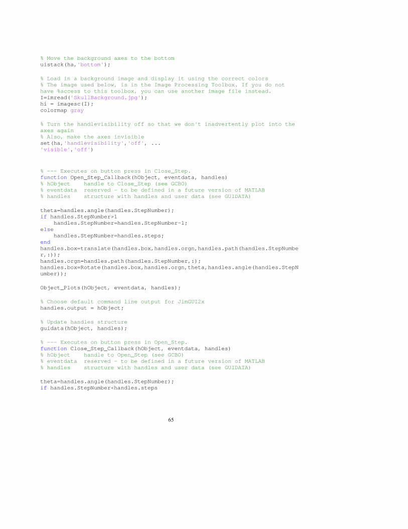
65

% Move the background axes to the bottom uistack(ha,'bottom'); % Load in a background image and display it using the correct colors % The image used below, is in the Image Processing Toolbox. If you do not have %access to this toolbox, you can use another image file instead. I=imread('SkullBackground.jpg'); hi = imagesc(I); colormap gray % Turn the handlevisibility off so that we don't inadvertently plot into the axes again % Also, make the axes invisible set(ha,'handlevisibility','off', ... 'visible','off') % --- Executes on button press in Close_Step. function Open_Step_Callback(hObject, eventdata, handles) % hObject handle to Close_Step (see GCBO) % eventdata reserved - to be defined in a future version of MATLAB % handles structure with handles and user data (see GUIDATA) theta=handles.angle(handles.StepNumber); if handles.StepNumber>1 handles.StepNumber=handles.StepNumber-1; else handles.StepNumber=handles.steps; end handles.box=translate(handles.box,handles.orgn,handles.path(handles.StepNumber,:)); handles.orgn=handles.path(handles.StepNumber,:); handles.box=Rotate(handles.box,handles.orgn,theta,handles.angle(handles.StepNumber)); Object_Plots(hObject, eventdata, handles); % Choose default command line output for JimGUI2x handles.output = hObject; % Update handles structure guidata(hObject, handles); % --- Executes on button press in Open_Step. function Close_Step_Callback(hObject, eventdata, handles) % hObject handle to Open_Step (see GCBO) % eventdata reserved - to be defined in a future version of MATLAB % handles structure with handles and user data (see GUIDATA) theta=handles.angle(handles.StepNumber); if handles.StepNumber<handles.steps

66

handles.StepNumber=handles.StepNumber+1; else handles.StepNumber=1; end handles.box=translate(handles.box,handles.orgn,handles.path(handles.StepNumber,:)); handles.orgn=handles.path(handles.StepNumber,:); handles.box=Rotate(handles.box,handles.orgn,theta,handles.angle(handles.StepNumber)); Object_Plots(hObject, eventdata, handles); % Choose default command line output for JimGUI2x handles.output = hObject; % Update handles structure guidata(hObject, handles); function Object_Plots(hObject, eventdata,handles) % Function to Plot Objects %PositionPlot axes(handles.PositionPlot) plot(handles.path(:,1),handles.path(:,2),'-k','LineWidth',2) hold on plot(handles.box(:,1),handles.box(:,2),':m','LineWidth',2); hold on plot([handles.DV(1,1); handles.MDM(handles.StepNumber,4)], [handles.DV(2,1); handles.MDM(handles.StepNumber,5)],'-or','MarkerSize',8,'MarkerFaceColor','r','LineWidth',2) hold on plot([handles.DV(1,3); handles.MDM(handles.StepNumber,12)], [handles.DV(2,3); handles.MDM(handles.StepNumber,13)],'-om','MarkerSize',8,'MarkerFaceColor','m','LineWidth',2) hold on plot([handles.DV(1,5); handles.MDM(handles.StepNumber,20)], [handles.DV(2,5); handles.MDM(handles.StepNumber,21)],'-ob','MarkerSize',8,'MarkerFaceColor','b','LineWidth',2) hold on hold off set(gca, 'XLim',[-0.05 0.09],'YLim',[-0.10 0.05]) %Value Displays set(handles.PositionNumberDisplay,'String',num2str(handles.points(handles.StepNumber + 1,1))) set(handles.ArtSur_XCoor,'String',[num2str(handles.MDMmm(handles.StepNumber,1),'%10.5f') ' mm'])

67

set(handles.ArtSur_YCoor,'String',[num2str(handles.MDMmm(handles.StepNumber,2),'%10.5f') ' mm']) set(handles.Angle_Blue,'String',[num2str(handles.angle(handles.StepNumber,1),'%10.2f') '°']) set(handles.PterygoidForceValue,'String',[num2str(handles.MDM(handles.StepNumber,6),'%10.2f') ' N']) set(handles.MasseterForceValue,'String',[num2str(handles.MDM(handles.StepNumber,14),'%10.2f') ' N']) set(handles.TemporalForceValue,'String',[num2str(handles.MDM(handles.StepNumber,22),'%10.2f') ' N']) set(handles.PterygoidLengthValue,'String',[num2str(handles.MDMmm(handles.StepNumber,9),'%10.3f') ' mm']) set(handles.MasseterLengthValue,'String',[num2str(handles.MDMmm(handles.StepNumber,17),'%10.3f') ' mm']) set(handles.TemporalLengthValue,'String',[num2str(handles.MDMmm(handles.StepNumber,25),'%10.3f') ' mm']) %{ set(handles.PterygoidRotationClose,'String',[num2str(handles.MDMrot(handles.StepNumber,11),'%10.3f') '°']) set(handles.MasseterRotationClose,'String',[num2str(handles.MDMrot(handles.StepNumber,19),'%10.3f') '°']) set(handles.TemporalRotationClose,'String',[num2str(handles.MDMrot(handles.StepNumber,27),'%10.3f') '°']) set(handles.PterygoidRotationOpen,'String',[num2str(handles.MDMrot(handles.StepNumber,10),'%10.3f') '°']) set(handles.MasseterRotationOpen,'String',[num2str(handles.MDMrot(handles.StepNumber,18),'%10.3f') '°']) set(handles.TemporalRotationOpen,'String',[num2str(handles.MDMrot(handles.StepNumber,26),'%10.3f') '°']) %} %Force Plot axes(handles.ForcePlot) plot(handles.SSS(:,1),handles.MDM(:,6),'-r','LineWidth',2) hold on plot(handles.SSS(handles.StepNumber,1),handles.MDM(handles.StepNumber,6),'ok','MarkerSize',8,'MarkerFaceColor','k') hold on plot(handles.SSS(:,1),handles.MDM(:,14),'-m') hold on plot(handles.SSS(handles.StepNumber,1),handles.MDM(handles.StepNumber,14),'ok','MarkerSize',8,'MarkerFaceColor','k') hold on plot(handles.SSS(:,1),handles.MDM(:,22),'-b') hold on plot(handles.SSS(handles.StepNumber,1),handles.MDM(handles.StepNumber,22),'ok','MarkerSize',8,'MarkerFaceColor','k') hold on hold off

68

set(gca,'xtick', [ ],'XLim',[38 92],'YLim',[-75 75]) %Length Plot axes(handles.LengthsPlot) plot([0.75; 0.75], [0; handles.MDMmm(handles.StepNumber,9)],'-r','LineWidth',6) hold on plot([2; 2], [0; handles.MDMmm(handles.StepNumber,17)],'-m','LineWidth',6) hold on plot([3.25; 3.25], [0; handles.MDMmm(handles.StepNumber,25)],'-b','LineWidth',6) hold on hold off set(gca,'xtick', [ ],'XLim',[0 4],'YLim',[0 120]) % Choose default command line output for JimGUI2x handles.output = hObject; % Update handles structure guidata(hObject, handles); % --- Executes on button press in OPENButton. function CloseButton_Callback(hObject, eventdata, handles) button_state = get(hObject,'Value'); % hObject handle to OPENButton (see GCBO) % eventdata reserved - to be defined in a future version of MATLAB % handles structure with handles and user data (see GUIDATA) while (handles.StepNumber < handles.steps) && (button_state == get(hObject,'Max')) if handles.StepNumber<handles.steps theta=handles.angle(handles.StepNumber); handles.StepNumber=handles.StepNumber+1; handles.box=translate(handles.box,handles.orgn,handles.path(handles.StepNumber,:)); handles.orgn=handles.path(handles.StepNumber,:); handles.box=Rotate(handles.box,handles.orgn,theta,handles.angle(handles.StepNumber)); end pause(0.1) Object_Plots(hObject, eventdata, handles); drawnow button_state = get(hObject,'Value');

69

end % Choose default command line output for JimGUI2x handles.output = hObject; % Update handles structure guidata(hObject, handles); % --- Executes on button press in CloseButton. function OpenButton_Callback(hObject, eventdata, handles) button_state = get(hObject,'Value'); % hObject handle to CloseButton (see GCBO) % eventdata reserved - to be defined in a future version of MATLAB % handles structure with handles and user data (see GUIDATA) while (1 < handles.StepNumber) && (button_state == get(hObject,'Max')) if 1<handles.StepNumber theta=handles.angle(handles.StepNumber); handles.StepNumber=handles.StepNumber-1; handles.box=translate(handles.box,handles.orgn,handles.path(handles.StepNumber,:)); handles.orgn=handles.path(handles.StepNumber,:); handles.box=Rotate(handles.box,handles.orgn,theta,handles.angle(handles.StepNumber)); end pause(0.1) Object_Plots(hObject, eventdata, handles); drawnow button_state = get(hObject,'Value'); end % Choose default command line output for JimGUI2x handles.output = hObject; % Update handles structure guidata(hObject, handles);

70

APPENDIX C

Equations

71

Variables in Force Analysis ACS Absolute Coordinate System T Location of temporal attachment on the mandible in the ACS M Location of mandible attachment on the mandible in the ACS P Location of pterygoid attachment on the mandible in the ACS, also the center of rotation C Location of centroid of the mandible in the ACS N Location that the normal force acts on the condyle in the ACS T0 Initial location of temporal attachment on the mandible in the ACS M0 Initial location of mandible attachment on the mandible in the ACS P0 Initial location of pterygoid attachment on the mandible in the ACS, also the center of rotation C0 Initial location of centroid of the mandible in the ACS N0 Initial location that the normal force acts on the condyle in the ACS Txp Location of T in the x direction relative to P Typ Location of T in the y direction relative to P Mxp Location of M in the x direction relative to P Myp Location of M in the y direction relative to P Nxp Location of N in the x direction relative to P Nyp Location of N in the y direction relative to P Ta Location of the temporal anchor point on the upper skull in the ACS Ma Location of the temporal anchor point on the upper skull in the ACS Pa Location of the temporal anchor point on the upper skull in the ACS TL Distance from P to T ML Distance from P to M CL Distance from P to C NL Distance from P to N DP Distance traveled by point P DT Distance traveled by point T DM Distance traveled by point M DL Distance traveled by point L X Translation of the mandible on the x axis Y Translation of the mandible on the y axis R Rotation of the mandible M Slope of articulating surface at N θT Positive angle from vertical axis between the Ta and T θM Positive angle from vertical axis between the Ma and M θP Positive angle from vertical axis between the Pa and P θN Positive angle from vertical axis between the N and P θTP Positive angle from horizontal axis between the T and P θCP Positive angle from horizontal axis between the C and P θMP Positive angle from horizontal axis between the M and P FT Force from temporal muscle FM Force from masseter muscle FP Force from pterygoid muscle FN Normal force from articulating surface µFN Friction force from articulating surface W Weight of mandible

72

Force Analysis and Equations

System Force Analysis

Σ Fx = 0Σ Fy = 0Σ Mo = 0

FN = Constant

•Statically IndeterminantoThree Muscle ForcesoNormal Force

•SolutionoForce Relationships

and Assumptions:

1

23

4 5

FP

FT

FN

μFN

W

FM

Points of Interest1. Contact Point2. Pterygoid Attachment3. Temporal Attachment4. Masseter Attachment5. Centroid

73

Bending Stress

GPaEwhereEI

FLcalculatedalsowasdeflectionThe

MPastrengthflexuralwhereDD

inertiaofmomentpolarI

IFLR

stress

diameterinnerDradiusouterRdiameterouterDlengthLforceF

io

o

io

o

07.23

:

)9.57(75.0)(64

3

44

==

≤−

==

==

=====

δ

σπ

σ

Attachment Points Calculated Diameters

Length m Outer radius m

Inner Radius m Force N Stress Mpa

Deflection m

Temporal Attachment 0.042 0.008 0.0015875 533.8 55.8395551 0.00198271 Temporal Anchor 0.029 0.007 0.0015875 533.8 57.6159723 0.00111468 Masseter Attachment 0.026 0.007 0.0015875 533.8 51.6556993 0.0008033 Pterygoid Attachment 0.021 0.0065 0.0015875 533.8 52.1573926 0.00056984 Pterygoid and Masseter Anchor 0.014 0.0065 0.0015875 533.8 34.7715951 0.00016884

74

APPENDIX D

75

ProE/Mechanica Mandible Model Properties Assuming Polycarbonate ABS Alloy (Estimated density from various materials)[36] VOLUME = 7.7202311e+04 MM^3 SURFACE AREA = 2.7034369e+04 MM^2 DENSITY = 1.3000000e-06 KILOGRAM / MM^3 MASS = 1.0036300e-01 KILOGRAM CENTER OF GRAVITY with respect to _LOWERJAW coordinate frame: X Y Z 6.0130673e+01 3.7984509e+01 4.2760339e+01 MM INERTIA with respect to _LOWERJAW coordinate frame: (KILOGRAM * MM^2) INERTIA TENSOR: Ixx Ixy Ixz 4.0597097e+02 -2.2923057e+02 -2.5805299e+02 Iyx Iyy Iyz -2.2923057e+02 7.0578962e+02 -1.3501130e+02 Izx Izy Izz -2.5805299e+02 -1.3501130e+02 6.6628517e+02 INERTIA at CENTER OF GRAVITY with respect to _LOWERJAW coordinate frame: (KILOGRAM * MM^2) INERTIA TENSOR: Ixx Ixy Ixz 7.7656536e+01 1.9606704e-03 1.1647505e-03 Iyx Iyy Iyz 1.9606704e-03 1.5939893e+02 2.8001351e+01 Izx Izy Izz 1.1647505e-03 2.8001351e+01 1.5859683e+02 PRINCIPAL MOMENTS OF INERTIA: (KILOGRAM * MM^2) I1 I2 I3 7.7656536e+01 1.3099366e+02 1.8700210e+02 ROTATION MATRIX from _LOWERJAW orientation to PRINCIPAL AXES: 1.00000 -0.00001 -0.00002 -0.00002 -0.70203 -0.71215 -0.00001 0.71215 -0.70203 ROTATION ANGLES from _LOWERJAW orientation to PRINCIPAL AXES (degrees): angles about x y z 134.590 0.000 0.000 RADII OF GYRATION with respect to PRINCIPAL AXES: R1 R2 R3 2.7816481e+01 3.6127533e+01 4.3165465e+01 MM

76

APPENDIX E

Financial Management

77

78

Parts Distributor Part Number Quantity Cost per Total Aluminum flat stock for motor clamps (6061 3/8T x 1 w x 6' L) McMaster-Carr 8975K47 1 $22.44 $22.44Aluminum flat stock for skull and motors (6061 3/8T x 6 w x 1' L) McMaster-Carr 8975K441 1 $19.15 $19.15Axle (Alloy 7075 Aluminum Precision Ground Rod 1/2" Diameter, 3' Length) McMaster-Carr 9063K163 1 $27.33 $27.33Base mount bearings (Stamped-Steel Mounted Ball Bearing--ABEC-1 2-Bolt Base Mount, for 1/2" Shaft Diameter) McMaster-Carr 5913K41 6 $10.95 $65.70Connecting cable (68pin X 2m controller to driver) National Instruments 186380-02 1 $135.00 $135.00Connecting cable (driver to motor) Automation Solutions MDC-AKM 3 $150.00 $450.00Controller (NI PCI-7344) National Instruments 778916-04 1 $1,349.10 $1,349.10Disc material (delrin film .003" Thick, 12" X 12") McMaster-Carr 5742T11 1 $9.93 $9.93Disc material (Slippery plastic selector pack) McMaster-Carr 5331K41 1 $34.88 $34.88Disc material (tape made with teflon PTFE 5yds x .5") McMaster-Carr 76025A711 1 $3.97 $3.97Disc material (teflon film Sheets Made Of Teflon®PTFE Adhesive Ready, .015" Thick, 6" X 6") McMaster-Carr 8711K91 1 $3.73 $3.73Driver (MDM2100) Automation Solutions MDM2100 1 $2,800.00 $2,800.00Frame end caps (1" X 1") McMaster-Carr 47065T91 25 $1.27 $31.75Mimics sofware Mimics v10.01 1 $4,000.00 $4,000.00Motor (2.2NM) Automation Solutions AKM33E 3 $695.00 $2,085.00Nut motor mount to motor (10-32 100pk) McMaster-Carr 90730A015 1 $7.81 $7.81Nut T-slot frame nuts (1/4-20 15pk) McMaster-Carr 47065T142 5 $9.16 $45.80Pulley (OD: 1.5" ID: .5"** will need boring to .55 ID) McMaster-Carr 6245K11 3 $3.50 $10.50Pulley (reduction Spoked for lower I OD: 8" ID: .5") McMaster-Carr 6245K55 3 $11.94 $35.82Screw bearing, motor mount, and motor clamp to frame (1/4-20 X 3/4 25pk) McMaster-Carr 98164A213 1 $9.48 $9.48Screw frame construction (Button Head 1/4-20 X 1-1/2" 50pk) McMaster-Carr 92949A546 1 $16.30 $16.30Screw motor clamp (10-32 X .75 box of pk25) McMaster-Carr 92185A991 1 $8.86 $8.86Screw motor mount to motor (10-32 X 7/8" 100pk) McMaster-Carr 92185A991 1 $13.41 $13.41Screw skull mount (1/4-20 X 1.25 10pk) McMaster-Carr 92185A544 1 $5.98 $5.98Skull SLA NEU 1 $500.00 $500.00String anchor (1/4 shoulder screw) McMaster-Carr 94035A532 6 $2.56 $15.36String guide pin (3/32 sholder screw) McMaster-Carr 99154A306 6 $4.43 $26.58T-slot frame (Fractional T-Slotted Framing System 1" X 1" Square Extrusion, 8' Length) McMaster-Carr 47065T123 4 $25.68 $102.72V-belt (4L Fractional hp Neoprene Rubber V-Belt Trade Size 4L310, 31" Outer Circle) McMaster-Carr 6191K25 3 $4.42 $13.26Washer for skull (.75 sq 1/4 bolt 10pk) McMaster-Carr 99041A103 1 $8.28 $8.28Washer frame construction ( .26ID 100pk) McMaster-Carr 92916A365 1 $6.91 $6.91

79

APPENDIX F Matlab Interface

80

Figure 55. Theoretical Mucle Force Profile

Figure 56. Muscle Lengths Comparison Plot

81

APPENDIX G Engineering Design Drawings

82

Bill Of Material

Quantity Part 2 T_SLOT_ALUM_20_MOTOR 3 AKM33 6 MOTOR_MOUNT_PLATE 3 PULLEY_1_HALF

19 1-4_20-75 51 560_WASHER 71 T_SLOT_NUT 12 10-32_75_BUTTON_HEAD 12 10-32_NUT 4 T_SLOT_ALUM_20 3 AXLE 6 BEARING

12 1-4_20-50 5 T_SLOT_ALUM_9_HALF 3 PULLEY_8 4 T_SLOT_ALUM_15 2 T_SLOT_ALUM_15_MOTOR 4 T_SLOT_ALUM_13 1 T_SLOT_ALUM_SKULL_POST 1 SKULL_SUPPORT 1 SKULL 6 10-32_SHOULDER_SCREW 6 2-56_SHOULDER_SCREW 1 SKULL_MOUNT_SPACER 8 1-4_20_1-75 3 MOTOR_CLAMP_TOP 6 MOTOR_CLAMP_SIDE 6 MOTOR_CLAMP_FOOT

28 10-32_75 32 1-4_20_X_125_BUTTON_HEAD 1 JAW_SUPPORT_BASE 2 JAW_SUPPORT_VERT 1 JAW_SUPPORT_ROD 2 JAW_SUPPORT_FINGER 7 10-32_SETSCREW 6 STRING_CLAMP 3 V-BELT 3 T_SLOT_GUSSET 6 1-4_20_50_SH

83

84

85

86

87

88

89

90

91

92

93

94

95

96

97

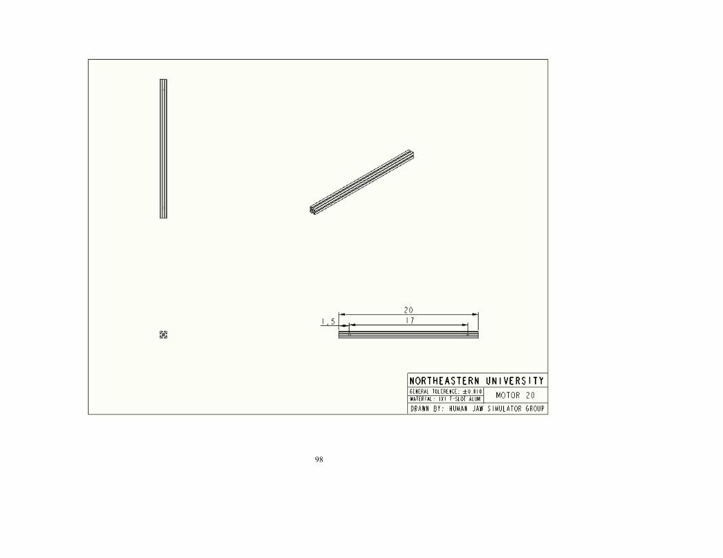
98

99

100

101

102

103

APPENDIX H LabVIEW Settings

104

NI Settings Documentation for Motion and Automation AXIS 1, 2, 3

1. Axis Configuration – Axis Configuration a. Type

i. Servo b. Enabled

i. Enabled c. Feedback

i. Encoder d. I/O Usage

i. Output: DAC Channel – 1 ii. Feedback: Encoder – 1

2. Motion I/O Settings

a. Limit Filters i. Enabled

b. Forward Limit Switch i. Enabled

ii. Active Low Polarity – originally supposed to be high polarity, but it trips the limit switches so it needs to be set to low polarity.

c. Reverse Limit Switch i. Enabled

ii. Active Low Polarity – originally supposed to be high polarity, but it trips the limit switches so it needs to be set to low polarity.

d. Home Switch i. Disabled

ii. Active Low Polarity e. Forward Software Limit

i. Disabled f. Reverse Software Limit

i. Disabled g. Inhibit Output Settings

i. Enabled ii. Active Low Polarity

h. Drive Ready i. (Not Applicable)

i. Inhibit Input Settings i. (Not Applicable)

3. Trajectory Settings – Trajectory Settings

a. Units i. Revolutions

b. Move Status Settings i. Following Error:

1. 32767 counts ii. Velocity Threshold

1. 5000 rpm iii. Run/Stop Threshold

1. 1 counts/sample c. Move Complete Criteria

i. Motor Off 1. Not Checked

105

ii. Run/Stop 1. Not Checked

iii. In Position 1. (Not Applicable)

iv. Delay 1. Not Checked

v. Deadband 1. Not Checked

vi. Minimum Pulse 1. 0 milliseconds

d. Velocity Filter Settings i. Filter Time

1. 10 milliseconds ii. Filter Distance

1. 100 steps

4. Trajectory Settings – Move Constraints a. Velocity

i. 200 rpm b. Acceleration

i. 100 rps/s c. Deceleration

i. 100 rps/s d. S Curve Time

i. 1 sample periods

5. Find Reference Settings - Home a. Initial Search Direction

i. Forward b. Final Approach Direction

i. Forward c. Home Edge to Stop On

i. Forward d. Approach Velocity %

i. 20 % velocity e. Offset Move

i. 0 steps f. Reset Position

i. Not Checked g. Smart Enable (Enable/Disable switches before executing Find Reference

i. Check Box

6. Find Reference Settings – Index a. Initial Search Direction

i. Forward b. Initial Search Direction

i. Forward c. Approach Velocity %

i. 20 % velocity d. Offset Move

i. 0 steps e. Reset Position

i. Not Checked f. Custom Search Distance

106

i. Not Checked g. Smart Enable (Enable/Disable switches before executing Find Reference

i. Check Box

7. Find Reference Settings – Forward Limit a. Initial Search Direction

i. NA b. Final Approach Direction

i. Into Limit c. Approach Velocity %

i. 20 % velocity d. Offset Move

i. 0 steps e. Reset Position

i. Not Checked f. Smart Enable (Enable/Disable switches before executing Find Reference

i. Check Box

8. Find Reference Settings – Reverse Limit a. Initial Search Direction

i. NA b. Final Approach Direction

i. Into Limit c. Approach Velocity %

i. 20 % velocity d. Offset Move

i. 0 steps e. Reset Position

i. Not Checked f. Smart Enable (Enable/Disable switches before executing Find Reference

i. Check Box 9. Find Reference Settings - Center

a. Initial Search Direction i. Forward

b. Final Approach Direction i. Into Limit

c. Approach Velocity % i. 20 % velocity

d. Offset Move i. 0 counts

e. Reset Position i. Not Checked

f. Smart Enable (Enable/Disable switches before executing Find Reference i. Check Box

10. Gearing Settings

a. Gear Master i. None

b. Gearing Mode i. Absolute

c. Gearing Enabled i. Disabled

d. Gear Ratio for Slave Axis

107

i. Numerator 1. 0

ii. Denominator 1. 1

11. Control Loop Settings – Control Loop Settings a. Kp

i. 10 b. Kd

i. 100 c. Ki

i. 10 d. Kv

i. 0 e. Nonlinear Gains

i. Derivative Sampling Period (Td) 1. 2

ii. Integration Limit (Lim) 1. 400

f. Feedforward Gains i. Velocity (Vff)

1. 0 ii. Acceleration (Aff)

1. 0 g. Control Loop Update Period

i. 250 microseconds

12. Control Loop Settings – Filter Settings a. Not Checked (Not Applicable)

13. Control Loop Settings – Torque Settings a. Primary DAC Output

i. Load Torque Limits & Offsets in: 1. Volts

ii. Positive Torque Limit 1. 10 Volts

iii. Negative Torque Limit 1. -10 Volts

iv. Torque Offset 1. 0 Volts

b. Secondary DAC Output i. Load Torque Limits & Offsets in:

1. Volts ii. Positive Torque Limit

1. 10 Volts iii. Negative Torque Limit

1. -10 Volts iv. Torque Offset

1. 0 Volts

14. Compare & Capture Settings a. Postion Breakpoints

i. Mode 1. Absolute

108

ii. Module 1. Not Checked

iii. Pulse Width 1. Not Checked

iv. Action 1. No Change

v. Window 1. 0 counts (steps)

vi. Active High Polarity 1. Checked

b. Trigger Inputs i. Low-to-High Edge

15. Digital I/O Settings

a. IO Port Direction i. Input

1. All Input Checked b. IO Port Active State

i. Active Low 1. All Active Low Checked

c. Output State i. No Change

1. All No Change Checked

d. IO Port Direction i. Input

1. All Input Checked e. IO Port Active State

i. Active Low 1. All Active Low Checked

f. Output State i. No Change

16. Digital I/O Settings – Port 1 a. IO Port Direction

i. Input 1. All Input Checked

b. IO Port Active State i. Active Low

1. All Active Low Checked c. Output State

i. No Change 1. All No Change Checked

d. IO Port Direction i. Input

1. All Input Checked e. IO Port Active State

i. Active Low 1. All Active Low Checked

f. Output State i. No Change

17. ADC Settings a. Channel

i. Enabled b. ADC Range

109

i. -10 to +10 Volts

18. ADC Channel 1 a. Channel

i. Enabled b. ADC Range

i. -10 to +10 Volts

19. Encoder Settings a. Encoder counts per revolution

i. 8192 – motors give line count of 2048, which needs to be multiplied by 4 in order to get counts per revolution

b. Filter Frequency i. 12.8 MHz

c. Encoder i. (Not Applicable)

d. Polarities i. Active High

1. A, B & Index Checked e. Index Reference Criteria

i. Inactive 1. A & B Checked

20. Encoder Settings – Encoder 1 a. Encoder counts per revolution

i. 8192 – motors give line count of 2048, which needs to be multiplied by 4 in order to get counts per revolution

b. Filter Frequency i. 12.8 MHz

c. Encoder i. (Not Applicable)

d. Polarities i. Active High

1. A, B & Index Checked e. Index Reference Criteria

i. Inactive 1. A & B Checked

21. PWM Settings

a. PWM i. Disabled

b. Clock Frequency i. 40 KHz

c. Load Duty Cycle in i. Percent

d. Duty Cycle i. 0 %

22. PWM Settings – PWM Output 1

a. PWM i. Disabled

b. Clock Frequency i. 40 KHz

c. Load Duty Cycle in

110

i. Percent d. Duty Cycle

i. 0 % 23. PWM Settings – PWM Output 2

a. PWM i. Disabled

b. Clock Frequency i. 40 KHz

c. Load Duty Cycle in i. Percent

d. Duty Cycle i. 0 %

111

112

APPENDIX I Gantt Chart

113

Gantt Chart Using Microsoft Project a Gantt chart was developed for planning and tracking the progress of the project. The majority of the tasks were completed on schedule while some were delayed for various reasons. Editing of the skull file took longer than initially planned since the mirroring function of the editing program was not available in the initial version. The mirror function was needed to complete editing of the skull file and the time it took to get access to the function pushed the task past its target completion date. The 3D printer then crashed twice when attempting to print the skull and an alternative printing source was used to print the skull. Once the skull was printed it was sent out for molding, but the company that was doing the molding had a rush order and the skull got pushed back. These delays combined resulting in the final skull being five weeks overdue. Additional late tasks were the creation of the list of materials and placing of the orders. These delays were caused by a lack of information on the control system and changes to the design. Since the parts took a week to be delivered and two weeks were planned for shipment this did not impact later tasks. Due to some of the details of the design, construction of the system took longer than initially planned, resulting in additional tasks being late. The task of completing the final LabVIEW program was also not completed on time. This was due to the fact that the controller that was delivered was for brushed DC servo motors while the model was using brushless DC servo motors. The controller had to be returned and the correct controller had to be created and shipped. Since this task was completed late it forced the tasks of connecting the model to the controls and the testing of the system to also be late.

114

115

116

117