Human Intracranial High Frequency Oscillation Detection ...
184
Grand Valley State University ScholarWorks@GVSU Masters eses Graduate Research and Creative Practice 8-2015 Human Intracranial High Frequency Oscillation Detection Using Time Frequency Analysis and Its Relation to the Seizure Onset Zone Riazul Islam Grand Valley State University Follow this and additional works at: hp://scholarworks.gvsu.edu/theses Part of the Biomedical Engineering and Bioengineering Commons is esis is brought to you for free and open access by the Graduate Research and Creative Practice at ScholarWorks@GVSU. It has been accepted for inclusion in Masters eses by an authorized administrator of ScholarWorks@GVSU. For more information, please contact [email protected]. Recommended Citation Islam, Riazul, "Human Intracranial High Frequency Oscillation Detection Using Time Frequency Analysis and Its Relation to the Seizure Onset Zone" (2015). Masters eses. 780. hp://scholarworks.gvsu.edu/theses/780
Transcript of Human Intracranial High Frequency Oscillation Detection ...

Grand Valley State UniversityScholarWorks@GVSU
Masters Theses Graduate Research and Creative Practice
8-2015
Human Intracranial High Frequency OscillationDetection Using Time Frequency Analysis and ItsRelation to the Seizure Onset ZoneRiazul IslamGrand Valley State University
Follow this and additional works at: http://scholarworks.gvsu.edu/theses
Part of the Biomedical Engineering and Bioengineering Commons
This Thesis is brought to you for free and open access by the Graduate Research and Creative Practice at ScholarWorks@GVSU. It has been acceptedfor inclusion in Masters Theses by an authorized administrator of ScholarWorks@GVSU. For more information, please [email protected].
Recommended CitationIslam, Riazul, "Human Intracranial High Frequency Oscillation Detection Using Time Frequency Analysis and Its Relation to theSeizure Onset Zone" (2015). Masters Theses. 780.http://scholarworks.gvsu.edu/theses/780

Human Intracranial High Frequency Oscillation Detection Using Time Frequency Analysis and Its
Relation to the Seizure Onset Zone
Riazul Islam
A Thesis Submitted to the Graduate Faculty of
GRAND VALLEY STATE UNIVERSITY
In
Partial Fulfillment of the Requirements
For the Degree of
Master of Science in Engineering
Biomedical Engineering
Seymour and Esther Padnos College of Engineering and Computing
August 2015

3
Dedication To my brother rifat, who will stay 17 forever…

4
Acknowledgements
I would first like to thank my thesis advisor Dr. Robert Bossemeyer for his guidance, expertise,
patience and time commitment throughout this entire project. Without his instructions full of
appreciations and inspirations, regular meetings and feedbacks, this work would not have been
completed. I cannot thank Dr. Paul Fishback enough for his continuous involvement with the
project, technical guidance, insight, and valuable time. I would also like to thank my committee
members Dr. Samhita Rhodes, and Dr. Konstantin Elisevich for their expertise and guidance.
Thanks a lot to Sergey Burnos for sharing his research findings with us. I owe countless thanks to
Dr. Mohamad Haykal, Epileptologist and Patti Sargent from EMU, for helping me understand
clinical epilepsy diagnosis procedure. I would like to thank Dr. Elisevich and Spectrum Health for
their research collaboration with Biomedical Engineering program at Grand Valley State University
(GVSU). I thank Dr. Shabbir Choudhuri for his continued support and encouragement throughout
my graduate study. Finally I would like to thank my parents Salma Akhter and Munsur Ali for their
continuous support and faith in me, and being very strong in their darkest of time.

5
Abstract
One third of the patients diagnosed with focal epilepsy do not respond to antiepileptic drugs. For
these patients the possible diagnosis options to give seizure freedom or at least reduce seizure
frequencies significantly would be surgical resection or seizure interrupting implantable devices. The
success of these procedures depends on accurate detection of the region causing seizure also known
as epileptic zone. This requires detail pre-surgical evaluation including Invasive Video
Electroencephalographic Monitoring (IVEM). The resulting great volume of intracranial
Electroencephalography (iEEG) signal is visually examined by an expert epileptologist which can be
time consuming, extremely complex, and not always effective. We have introduced an automated
method to help the epileptologist analyze the iEEG signals.
Literature suggest that signals recorded from brain regions subject to seizure activity produce a short
durational high gamma ripple activity in the iEEG called High Frequency Oscillations (HFOs). The
algorithm presented in this thesis uses an automated time-frequency space analysis method to detect
HFOs and distinguish them from high frequency artifacts. As HFOs are short-lived high frequency
oscillations, the time-frequency space analysis method chosen should have good time and frequency
resolution capabilities. The Stockwell transform was used for this purpose which is a variable
window version of the Short Time Fourier Transform (STFT). We have modified the detection
algorithm to analyze the multi-channel iEEG data obtained from patients monitored at the
Spectrum Health Epilepsy Monitoring Unit (EMU) and found that the electrode site recordings
exhibiting higher HFO rate are within the Seizure Onset Zone (SOZ) determined by visual
examination of the iEEG recordings by the epileptologist. These electrodes also continue to show
higher HFO rate throughout the entire study. The HFO analysis presented in this thesis suggests
that HFO detection and identification may be used to reduce IVEM monitoring time by aiding the

6
neurosurgeon delineating the epileptic zone in relatively shorter time. This will lead to better
surgical outcome or succesful implantation of the seizure intervention devices.

7
Table of Contents Dedication ..................................................................................................................................................... 3
Acknowledgements ....................................................................................................................................... 4
Abstract ......................................................................................................................................................... 5
List of Figures ................................................................................................................................................ 9
List of Tables ............................................................................................................................................... 13
List of Abbreviations ................................................................................................................................... 14
1. Introduction ........................................................................................................................................ 15
1.1. Problem and Clinical Significance ............................................................................................... 15
1.2. Specific Purpose .......................................................................................................................... 17
1.3. Objectives.................................................................................................................................... 18
1.4. Thesis Roadmap .......................................................................................................................... 18
2. Background and Literature Review ..................................................................................................... 19
2.1. Background ................................................................................................................................. 19
2.1.1. Brain Anatomy and Functions ............................................................................................. 19
2.1.2. Electroencephalogram (EEG) .............................................................................................. 21
2.1.3. Epilepsy ............................................................................................................................... 23
2.1.4. Epilepsy Diagnosis and Treatment ...................................................................................... 25
2.1.5. High Frequency Oscillations Defined .................................................................................. 28
2.2. Literature Review ........................................................................................................................ 31
3. Methodology ....................................................................................................................................... 36
3.1. Patient Selection ......................................................................................................................... 36
3.2. Privacy Statement ....................................................................................................................... 37
3.3. Electrode types and implantation sites ...................................................................................... 37
3.4. Data acquisition .......................................................................................................................... 37
3.5. Limitations................................................................................................................................... 38
3.6. Data analysis ............................................................................................................................... 38
3.7. Proposed HFO detection algorithm ............................................................................................ 39
3.7.1. Stage 1: Detection of EoIs ................................................................................................... 39
3.7.2. Stage 2: Recognition of HFOs among EoIs .......................................................................... 41
3.7.3. Stockwell (S) Transformation .............................................................................................. 42
3.7.4. Definition of the HFO region ............................................................................................... 49
4. Results ................................................................................................................................................. 50

8
4.1. Example data ............................................................................................................................... 50
4.2. Analysis of Spectrum Health Epilepsy Monitoring Unit Data ..................................................... 60
4.2.1. Patient ID: WDH-022 ........................................................................................................... 60
4.2.2. Patient ID- SH-EEG .............................................................................................................. 83
5. Discussion ............................................................................................................................................ 91
6. Future work ......................................................................................................................................... 95
7. Conclusion ........................................................................................................................................... 96
8. Bibliography ............................................................................................................................................ 97
9. Appendices ............................................................................................................................................ 102
9.1. Appendix A: Clinical Events and EEG Correlation for Patient WDH-022 ........................................ 102
9.2. Appendix B: Electrode Locations for Patient – SH-EEG .................................................................. 110
9.3. Appendix C: HFO Analysis Tool ...................................................................................................... 116
9.3.1. Operating Manual: .................................................................................................................. 116
9.3.2. MATLAB Scripts ....................................................................................................................... 118
9.4. Appendix D: HFOs Detected During Seizure .................................................................................. 141

9
List of Figures Figure 2.1: Anatomy of a human brain ......................................................................................................... 20
Figure 2.2: (a) Layer of Cortex [34] (b) Pyramidal neurons [45] ............................................................... 20
Figure 2.3: (a) Human hippocampus located in the medial temporal lobe of brain [46] (b) Basic
circuit of the hippocampus sketched by Ramon y Cajal [45] ............................................................ 21
Figure 2.4: (a) Electrode placement to monitor EEG (b) Origin of the EEG potential [34] .............. 22
Figure 2.5: Intracranial EEG electrode placement [38] ............................................................................. 23
Figure 2.6: Localized electrodes in a patient with bilateral grids and multiple strips implanted [39] .. 26
Figure 2.7: Subdural strip with eight electrodes [40]................................................................................... 27
Figure 2.8: A 64 contacts grid electrode [40] ............................................................................................... 27
Figure 2.9: A depth electrode with 8 contact points [41] ........................................................................... 28
Figure 2.10: Microelectrode array [42] .......................................................................................................... 28
Figure 2.11: HFO waveform and spectral frequency variability (A) Ripple (B) Fast ripple ................. 29
Figure 2.12: Intracranial EEG signal with spike and wave [15] ................................................................ 30
Figure 2.13: Intracranial EEG signal showing an epileptic seizure [44] .................................................. 30
Figure 3.1: Data Acquisition system (Spectrum Health EMU) ................................................................. 38
Figure 3.2: Importing EEG data to MATLAB environment .................................................................... 39
Figure 4.1: (a) 30 s example iEEG data sampled at 2000 Hz (b) Example data after 80 to 488 Hz
band-pass filtering ................................................................................................................................... 50

10
Figure 4.2: Validation showing the 4th HFO detected in the 30 s example iEEG data ....................... 53
Figure 4.3: Example published in Burnos, et. al., of a HFO in a temporomesial recording. ............... 54
Figure 4.4: Simulated HFO event in time domain ...................................................................................... 56
Figure 4.5: (a) Sample raw iEEG data before adding the simulated HFO event (b) iEEG data after
band-pass filtering, red arrow shows the point where the simulated HFO will be added ............ 56
Figure 4.6: (a) Sample 30 s raw iEEG data after adding the simulated HFO event at (b) iEEG signal
with the simulated event after band-pass filtering. ............................................................................. 57
Figure 4.7: (a) Raw iEEG signal after adding the simulated HFO (b) 8 HFO events detected in the
Band-pass filtered iEEG signal ............................................................................................................. 58
Figure 4.8: Simulated HFO event detected by the detection algorithm .................................................. 59
Figure 4.9: Total HFO count for period from 14:07 to 16:07 with green arrows indicating channels
that comprise the HFO region .............................................................................................................. 62
Figure 4.10: Total HFO count for period from 14:07 to 16:07with green arrows indicating channels
comprising the HFO region and red arrows showing the epileptologist‘s channels of interest .. 63
Figure 4.11: HFO rate over time 12:06 to 14:07 and seizure-1 occurring at 12:57:12 ........................... 64
Figure 4.12: HFO rate over time 12:06 to 14:07 and seizure-2 occurring at 13:16:02 ........................... 64
Figure 4.13: HFO rate over time 14:07 to 16:07 and seizure-3 occurring at 14:14:03 ........................... 65
Figure 4.14: HFO rate from 14:07 to 16:07 and seizure-4 to 8 occurring between 14:27 to 14:34 ..... 66
Figure 4.15: HFO rate over time 16:07 to 18:07 and seizure-9 occurring at 17:51 and seizure 10 to 14
occurring between 18:00 to 18:07 ......................................................................................................... 67
Figure 4.16: HFO rate over time 18:07 to 20:07 and seizure-15 occurring at 19:10 .............................. 68

11
Figure 4.17: HFO rate over time from 12:06 to 20:07 ............................................................................... 69
Figure 4.18: HFO plotted for electrode B-2, approximate time 15:03. The frequencies recorded at
the peak of the EoI are, HFO peak at 106 Hz, trough at 68 Hz and a low frequency peak at 27
Hz............................................................................................................................................................... 71
Figure 4.19: HFO plotted for electrode B-3, approximate time 14:26. The frequencies recorded at
the peak of the EoI are, HFO peak at 112 Hz, trough at 52 Hz and a low frequency peak at 40
Hz............................................................................................................................................................... 72
Figure 4.20: HFO plotted for electrode B-4, approximate time 14:28. The frequencies recorded at
the peak of the EoI are, HFO peak at 119 Hz, trough at 41 Hz and a low frequency peak at 28
Hz............................................................................................................................................................... 73
Figure 4.21: HFO plotted for electrode C-11, approximate time 14:41. The frequencies recorded at
the peak of the EoI are, HFO peak at 127 Hz, trough at 85 Hz and a low frequency peak at 29
Hz............................................................................................................................................................... 74
Figure 4.22: HFO plotted for electrode C-12, approximate time 14:15. The frequencies recorded at
the peak of the EoI are, HFO peak at 120 Hz, trough at 73 Hz and a low frequency peak at 56
Hz............................................................................................................................................................... 75
Figure 4.23: HFO plotted for electrode C-18, approximate time 14:15. The frequencies recorded at
the peak of the EoI are, HFO peak at 136 Hz, trough at 87 Hz and a low frequency peak at 10
Hz............................................................................................................................................................... 76
Figure 4.24: HFO plotted for electrode C-19, approximate time 14:42. The frequencies recorded at
the peak of the EoI are, HFO peak at 126 Hz, trough at 60 Hz and a low frequency peak at 28
Hz............................................................................................................................................................... 77
Figure 4.25: HFO plotted for electrode D-1, approximate time 14:49. The frequencies recorded at
the peak of the EoI are, HFO peak at 115 Hz, trough at 64 Hz and a low frequency peak at 14
Hz............................................................................................................................................................... 78
Figure 4.26: HFO plotted for electrode D-2, approximate time 14:30. The frequencies recorded at
the peak of the EoI are, HFO peak at 110 Hz, trough at 63 Hz and a low frequency peak at 35
Hz............................................................................................................................................................... 79
12
Figure 4.27: HFO plotted for electrode D-5, approximate time 14:19. The frequencies recorded at
the peak of the EoI are, HFO peak at 111 Hz, trough at 80 Hz and a low frequency peak at 42
Hz............................................................................................................................................................... 80
Figure 4.28: HFO plotted for electrode D-14, approximate time 14:29. The frequencies recorded at
the peak of the EoI are, HFO peak at 114 Hz, trough at 82 Hz and a low frequency peak at 49
Hz............................................................................................................................................................... 81
Figure 4.29: HFO rate determined for 14:07 to 16:07 for different amplitude threshold value of ..... 82
Figure 4.30: Total number of HFO detected over a 2 hours of study. The green arrow point the
channels with higher HFO and the red arrow shows the channels which can be the possible
SOZ. .......................................................................................................................................................... 84
Figure 4.31: HFO rate over time from 19:09 to 03:09 with 1 minute window at a time and 30
seconds overlap ........................................................................................................................................ 86
Figure 4.32 : HFO plotted for electrode C-34, approximate time 20:50. The frequencies recorded at
the peak of the EoI are, HFO peak at 94 Hz, trough at 40 Hz and a low frequency peak at 28
Hz............................................................................................................................................................... 87
Figure 4.33: HFO plotted for electrode D-39, approximate time 19:49. The frequencies recorded at
the peak of the EoI are, HFO peak at 96 Hz, trough at 42 Hz and a low frequency peak at 22
Hz............................................................................................................................................................... 88
Figure 4.34: HFO plotted for electrode D-40, approximate time 19:41. The frequencies recorded at
the peak of the EoI are, HFO peak at 100 Hz, trough at 60 Hz and a low frequency peak at 39
Hz............................................................................................................................................................... 89

13
List of Tables Table 1.1: Objectives of the study ................................................................................................................. 18
Table 2.1: EEG rhythm frequency ranges [34] ............................................................................................ 22
Table 2.2: Generalized seizures and their symptoms [35]. ......................................................................... 24
Table 2.3: Common criteria for epilepsy surgery [47] ................................................................................ 25
Table 4.1: The description of the 7 HFO events detected by the algorithm .......................................... 51
Table 4.2: The description of the 8 HFO events detected by the algorithm .......................................... 58
Table 4.3: Information of the first patient analyzed in our study ............................................................. 60
Table 4.4: Description of the Electrode Placement .................................................................................... 61
Table 4.5: Epileptologist‘s dictation regarding EEG signal during Seizure 1 and 2 (day 1) ................. 65
Table 4.6: Epileptologist‘s dictation regarding EEG signal during Seizure 3 to 8 (day 1) .................... 66
Table 4.7: Epileptologist‘s notes regarding EEG signal during Seizure 9 to 15 (day 1) ........................ 68
Table 4.8: Information of the second subject of our study ....................................................................... 83
Table 4.9: Electrode Grids and strips used for patient - SH-EEG .......................................................... 83
Table 4.10: Epileptologist‘s note about the first three seizure events (day 1) ......................................... 85

14
List of Abbreviations
SOZ : Seizure Onset Region
EZ : Epileptic Zone
HFO : High Frequency Oscillation
EoI : Event of Interest
IES : Interictal Epileptiform Spike
EEG : Electroencephalography
iEEG : intracranial Electroencephalography
MRI : Magnetic Resonance Imaging
fMRI : Functional Magnetic Resonance Imaging
CT : Computed Tomography
PET : Positron Emission Tomography
AED : Anti-Epileptic Drug
MTLE : Mesial Temporal Lobe Epilepsy
EMU : Epilepsy Monitoring Unit
IIR : Infinite Impulse Response
FIR : Finite Impulse Response
WT : Wavelet Transform
STFT : Short Time Fourier Transform
HiFP : High frequency peak
LoFp : Low frequency peak
PSD : Power Spectral Density

15
1. Introduction
1.1. Problem and Clinical Significance
The word epilepsy is derived from Greek word epilambanein, which means ‗to seize‘ or ‗to attack‘. It
was first recorded in the West as part of a Babylonian cuneiform treatise, known as ‗Sakikku‘ or ‗all
diseases‘ on tablets dating from 716 BC to 612 BC. It is the most common serious neurological
condition affecting nearly 70 million people in the world. In high-income countries, approximately 6
per 1000 people will develop epilepsy during their lifetime [1]. The annual direct medical care cost of
epilepsy in the United States is $9.6 billion, which does not include other indirect costs like inferior
quality of life and lost in earnings [14].
Most patients with epilepsy have a favorable prognosis, but around 25% continue to have seizures
with varying degree of frequency even after medication and/or focal resection of brain tissue [2].
Despite tremendous advances in surgical technology and antiepileptic drug therapy the proportion
of epilepsy patients without viable treatment has remained constant over the last 15 years [3]. To
avoid this therapeutic plateau, a great deal of focus has been put into alternative devices designed to
detect, predict, prevent, and terminate seizures. One of the promising alternatives is the Neuropace
closed loop stimulator. However, among the participants of a recent clinical trial, only 14.5%
enjoyed a seizure-free period of 6 months or more [12]. This suggests that the ultimate success of a
resection surgery or implantable device depends on better understanding of where, when, how the
seizure originates and spreads, and the timely and accurate detection of the Seizure Onset Zone
(SOZ) [4].

16
EEG signal recorded during a routine epilepsy pre-surgical study can now be sampled digitally and
analyzed automatically to generate quantitative measures of the signals. This ―quantitative EEG‖ is
already available in many commercial systems including Nihon Kohden Neurofax system that is
used by the Spectrum Health Epilepsy Monitoring Unit which allows high frequency multi-channel
recording. As a PC-supported EEG system, their EEG-1200 system enables registration, evaluation
and analysis of EEG and polygraphic data. The system can record up to 256 channels at sampling
rates of up to 10,000 Hz. It also has a software-controlled switch box for intracranial stimulation
[13] which is used for functional mapping of the cortex and identification of critical cortical
structures [59].
With the development of EEG recording technology (electrodes, amplifier etc.), high bandwidth
epilepsy study is now possible and this unveils many new possibilities in EEG study for epilepsy. A
very intriguing phenomenon that appears to be strongly related to epilepsy is that of High Frequency
Oscillations (HFOs) [3]. Recent progress in high bandwidth intracranial EEG recording has made it
possible to examine high frequency components. Experimental and clinical data suggest that more
localized HFOs occur far beyond the spectral frequency limits of traditional EEG which are from
0.1Hz to 50 Hz. For example, hippocampal ripples 100—200 Hz or fast-ripples 250—500 Hz may
be an electrical signature of focal epilepsy during seizure-free states [6, 8]. Studies revealed that
HFO may also play an initiating role in seizure generation [7].
In this thesis we demonstrated the applicability of an automated HFO detection method [5] in
clinical epilepsy monitoring. HFOs are short durational high gamma ripple activity in EEG signal.
The usual duration of HFOs are 10-100ms and frequency ranges within 30-600 Hz [8]. Since visual
marking of HFO is very time consuming, several semi-automated and automated methods have
been proposed including Wavelet transform method and Short-time Fourier transform method [9].

17
The automated detection algorithm used in this thesis applies a Time Frequency Analysis method to
detect HFO and to visualize them. The earliest HFO detectors relied only on time domain, a
number of recent detectors also incorporate frequency domain although it is computationally more
demanding. Frequency domain analysis helps to differentiate HFOs from high frequency
interference such as sharp artifact, Interictal Epileptiform Spike (IES), and other artifacts which are
not distinguishable in time domain [5]. The automated HFO detection method used in this study
detects the HFO in two stages. The first stage is Event of Interests (EoIs) detection, which locates
potential HFO candidates using time domain measures. In the second stage, instantaneous power
spectral density of an EoI is analyzed [5]. The HFO appears as a short-lived event with an isolated
spectral peak at a distinct frequency [10, 11]. This criteria is used in the second stage to differentiate
HFOs from artifacts similar to HFOs (e.g. sharp artifacts, Interictal Epileptiform Spike (IES)
without HFO) [5].
1.2. Specific Purpose
The purpose of this research study is to understand HFO generated by epileptic brain, validate the
HFO detection algorithm developed by Burnos, et al. [5], and finally modify it to apply on iEEG
data obtained from EMU. Our implementation of this detection algorithm was validated using the
example data obtained from these authors and verified using a simulated HFO event. Later the
algorithm was applied to iEEG data recorded during pre-surgical monitoring performed at Spectrum
Health Epilepsy Monitoring Unit (EMU) to investigate the relationship of HFO rates in different
electrode recording sites and the Seizure Onset Zone (SOZ) determined by the epileptologist.
Another goal of the research is to observe how HFO rate changes over time.

18
1.3. Objectives
The specific objectives which will be fulfilled at the end of the study are provided in Table 1.1.
Table 1.1: Objectives of the study
Objectives
Understand the characteristics of HFOs
Create a simulated HFO
Validate the HFO detection algorithm developed by Burnos, et. al. [5] by detecting the simulated HFO
Apply the detection algorithm on example data provided by the authors and confirm the results agree with those of the authors.
Modify the algorithm for the data collected from EMU
Use the HFO detection algorithm to determine the total number of HFOs over a fixed time interval.
Compare the correlation between the channels with higher HFO rates with the Seizure Onset Zone (SOZ) found by epileptologist
Determine HFO rate over time and investigate the results to see how HFO rates change over time
1.4. Thesis Roadmap
The thesis is organized in the following manner. Chapter 2 discusses the background, definitions
and scientific literature related to epilepsy, EEG and HFO. The goal of this section is to give the
reader a brief idea about the background and rationale of the thesis. The third chapter describes the
data collection method, details about the proposed algorithm and the method used to perform
analysis. This section also discusses the procedure followed to generate the results. The result
section will present the findings analyzing the sample data provided by Burnos, et. al. [5], simulated
HFO signal and data collected from Spectrum Health Epilepsy Monitoring Unit. The

19
epileptologist‘s notes and findings will also be presented in this section. Finally the findings will be
discussed and conclusion will be made.
2. Background and Literature Review
2.1. Background
This multidisciplinary research requires the knowledge of both brain anatomy and signal processing
techniques. The signal processing technique used will be discussed in detail in methodology section.
This section will provide a concise background of clinical epilepsy diagnostic steps and their
relevance in epilepsy treatment. Also, the purpose was to make the reader familiar with steps and
procedures followed before going for a resection surgery. As throughout the thesis different brain
anatomy and their functions will be mentioned in numerous occasions, a relevant brain anatomical
background is presented here.
2.1.1. Brain Anatomy and Functions
The adult human brain weighs about 1500 g. In the Figure 2.1[34] the largest visible brain region is
the cerebrum and its surface looks folded. The brain has two hemispheres, each of which is divided
into frontal, parietal, occipital, and temporal lobes. The higher cerebral functions, are accurate
sensations and voluntary motor control of muscles.

20
Figure 2.1: Anatomy of a human brain
The cerebrum surface has six layers, consisting of pyramidal neurons and interneurons, and glia
(supporting cells). Figure 2.2 (a) shows the layers of cortical surface. The cortex is formed by
interconnected columns of several thousand neurons arranged perpendicular to the cortical surface.
Stimulation of these columns in motor cortex produce coordinated movement by activating muscles.
Figure 2.2 (b) shows a closer look at the pyramidal neurons. They are also found in hippocampus
and amygdala.
Figure 2.2: (a) Layer of Cortex [34] (b) Pyramidal neurons [45]
Hippocampus means seahorse in Greek. Shown in Figure 2.3 (a) it looks like a seahorse due to the
way it is folded during development. Located under the cerebral cortex, it is a major component of
human brain. Figure 2.3 (b) shows the basic circuitry of a human hippocampus. By interacting with

21
different components and neighboring regions, the hippocampus circuit plays a very important role
in consolidation of information from short-term memory to long-term memory and spatial
navigation [47]. Hippocampal tissue damage is often observed in temporal lobe epilepsy [57]. It also
has a close relationship with HFOs, which will be discussed later.
Figure 2.3: (a) Human hippocampus located in the medial temporal lobe of brain [46] (b) Basic circuit of the hippocampus sketched by Ramon y Cajal [45]
2.1.2. Electroencephalogram (EEG)
EEG is the recording of electrical activity within the brain. EEG recording in general can refer to
scalp or intercranial. The generator sources for scalp EEG waves are within the cerebral cortex. The
electrical activity is produced by voltage fluctuations resulting from ionic current flows due to neural
activity of the brain. It consists of the summed electrical activities of populations of neurons, with a
modest contribution from glial cells. The neurons are excitable cells with characteristic intrinsic
electrical properties, and their activity produces electrical and magnetic fields. These fields may be
recorded by means of electrodes at a short distance from the sources, or from the cortical surface, or
at longer distances, even from the scalp [1, 23]. Figure 2.4 (a) shows placement of electrodes for a
typical scalp EEG study and Figure 2.4 (b) shows how electrode measures voltage difference at the
scalp which represents ―spatial averaging‖ of electrical activity from a limited area of cortex.
Individual action potentials are not the main contributor to scalp EEG activity. Synaptic potential is
the difference in potential between the inside and outside of a postsynaptic neuron. They are of
22
much lower voltage than action potentials, but the produced current has a much larger Effect on the
EEG because there are many more synapses than neurons. Postsynaptic potentials also have a
longer duration and involve a larger amount of membrane surface area than action potentials [34].
Figure 2.4: (a) Electrode placement to monitor EEG (b) Origin of the EEG potential [34]
Small metal discs called electrodes are positioned in a standardized pattern on the scalp to record the
signal. The signals from these electrodes are often referred as EEG channels. EEG signals are
typically recorded from more than one location using multiple electrodes and called a multi-channel
EEG study. EEG rhythms correlate with patterns of behavior (level of attentiveness, sleeping,
waking, seizures, and coma). EEG rhythm frequency ranges are provided in Table 2.1
Table 2.1: EEG rhythm frequency ranges [34]
Rhythm Frequency Range and activity
Gamma 20-60 Hz (―cognitive‖ frequency band)
Beta 14-20 Hz (activated cortex)
Alpha 8-13 Hz (quiet waking)
Theta 4-7 Hz (sleep stages)
Delta less than 4 Hz (sleep stages, especially ―deep sleep‖)

23
Intracranial EEG (iEEG) is an invasive procedure to measure the electrical activity of brain. In this
procedure electrodes are placed inside the brain through surgery. iEEG not only helps to record
slight changes in brain activity but it is also suitable for long durational EEG recording. Intracranial
EEG monitoring places the electrode closer to the site of neural activity enabling a more precise
monitoring of seizure activity and locating the area of the brain where the seizures originate. This
involves an operation under general anesthetic to remove part of the skull and place electrodes
either on the surface or deep within the brain. These electrodes are attached to a video
electroencephalogram monitor and both the video of patient movements and the multi-channel
EEG are monitored continuously for five to ten days. Intracranial monitoring also facilitates
functional of brain electrical activity with specific response. This allows the medical team to check
areas of the brain needed for essential tasks, such as speech and movement. This is important to
know, as it indicates whether resection surgery would put these functions at risk [39]. Figure 2.5
shows a surgical procedure that has placed an intracranial electrode array on the surface of the brain
after part of the skull has been removed.
Figure 2.5: Intracranial EEG electrode placement [38]
2.1.3. Epilepsy
According to a definition proposed by the Mayo Clinic, Epilepsy is a central nervous system
disorder (neurological disorder) in which the nerve cell activity in the brain is disturbed, causing a

24
seizure, during which an individual may experience abnormal behavior, symptoms and sensations,
including loss of consciousness. Seizure symptoms vary person to person. Physicians generally
classify seizures as either focal or generalized, based on how the abnormal brain activity begins.
(1) Focal Seizures: According to the Mayo Clinic [35], focal seizures appear to originate from
abnormal activity in only one area of the brain. They fall under two categories.
(a) Simple partial seizures: They do not cause loss of consciousness but might alter
emotions or change the way things look, smell, feel, taste or sound. Simple partial
seizures may also result in involuntary jerking of a body part, such as an arm or leg, and
spontaneous sensory symptoms such as tingling, dizziness and flashing lights.
(b) Complex partial seizures: These seizures involve a change or loss of consciousness or
awareness. During a complex partial seizure, the patient may stare into space and not
respond normally to the environment or perform repetitive movements, such as hand
rubbing, chewing, swallowing or walking in circles [35].
(2) Generalized seizures: Seizures that appear to involve all areas of the brain are called
generalized seizures. Six types of generalized seizures exist are described in Table 2.2.
Table 2.2: Generalized seizures and their symptoms [35].
Generalized seizures Symptoms
Absence seizures Staring into space or subtle body movements such as eye blinking or lip
smacking.
Tonic Seizures Affect muscles in the back, arms and legs and may cause one to fall to
the ground.
Atonic Seizures Cause a loss of muscle control.
Clonic Seizures Associated with repeated or rhythmic, jerking muscle movements
Myoclonic Seizures Usually appear as sudden brief jerks or twitches of arms and legs.
Tonic-clonic
seizures
Also known as grand mal seizures. Can cause an abrupt loss of
consciousness, body stiffening and shaking, and sometimes loss of
bladder control or biting of tongue.

25
2.1.4. Epilepsy Diagnosis and Treatment
The prognosis of epilepsy is generally good. Approximately two-thirds of patients are rendered
seizure free by treatment with antiepileptic drugs (AEDs). Although the number of AEDs is
growing, one-in-three of those diagnosed do not respond to AEDs and continue to experience
seizures with varying degrees of frequency and severity [14]. These patients suffer from what is
called refractory epilepsy. Commonly used options for treating those with debilitating refractory
epilepsy include vagus nerve stimulation, deep brain stimulation, the ketogenic diet, and epilepsy
surgery [14, 36].
Phase 1 for epilepsy treatment includes preliminary tests before surgery. This includes non-invasive
scalp EEG and neuropsychological tests to help find the affected area of brain. A psychiatrist may
see the patient to help determine how epilepsy affects their quality of life. Anticonvulsant
medications are removed during these phase to promote seizure. Only a few thousand epilepsy
surgeries are performed each year due to limitations in knowledge regarding the root cause of
epilepsy, availability of resources, cost, and strict criteria [14]. Common criteria that must be met by
candidates for epilepsy surgery according to the Epilepsy Foundation are summarized in Table 2.3
Table 2.3: Common criteria for epilepsy surgery [47]
Criteria
Diagnosis of epilepsy is secure
Failure of at least two AEDs in controlling seizures
Onset site can be localized (Focal epilepsy)
Epileptogenic Focus can be safely removed
Understanding of benefits/risks and desires surgery
For the Phase 2 treatment procedure, the patients agree to surgery for placing electrodes in the brain
to receive clearer and more accurate information about seizure. After the surgery the patients are

26
usually given a one or two day period to recover. Then the electrodes are connected with EEG and
video monitoring unit. This period can last a week or even more. In this phase the epileptologist
attempts to acquire enough information to find the origin of the seizure. Then the patients may
choose a surgery to remove the part of the brain causing seizures. There are three main types of
intracranial EEG electrodes used in clinical practice. They are strip, grid, and depth electrodes.
Seizure manifestation, MRI scan, scalp EEG performed during Phase I treatment stage provide
physicians with an approximate idea about the location of seizure origin. They consider the anatomy
of the location and decide what type electrode combination will be most suitable for seizure
localization with minimal invasion.
The information from these intracranial electrode arrays is used to localize ictal onset zones, which
are then the targets of surgical resection. Often after surgical implantation MRI scan is conducted to
accurately locate the electrodes [39]. Magnetic Resonance Imaging (MRI) is a technique that uses a
magnetic field and radio waves to create detailed images of the organs and tissues within body.
Figure 2.6 shows reconstructed brain anatomical model of localized electrodes in a patient with
bilateral grids (red) and strip electrodes (blue) implanted.
Figure 2.6: Localized electrodes in a patient with bilateral grids and multiple strips implanted [39]

27
Strip electrodes are multiple electrodes aligned and attached to a strip of backing material. These
electrodes are implanted in the subdural cortical layer of the brain to record electrical activity on the
cortical surface. They are used when the region to be studied is small. Figure 2.7 shows strip
electrode with 8 pins.
Figure 2.7: Subdural strip with eight electrodes [40]
Grid electrodes (Figure 2.8) are multiple strip electrodes attached with one another and form a
rectangular grid and implanted in the subdural cortical layer of the brain to record electrical activity.
Grid electrodes are used to evaluate larger surface areas.
Figure 2.8: A 64 contacts grid electrode [40]
Depth electrodes look like a single thin wire. They usually have multiple contact point throughout
their entire length. These electrodes may be used to access structures deep within the brain, such as
the amygdala and the hippocampus. They are placed deep in the brain to detect seizure activity that
cannot be recorded from the surface of the brain. Figure 2.9 shows sample depth electrodes with 8
contact points. So this electrode will record EEG signal from 8 different depth locations of brain.

28
Figure 2.9: A depth electrode with 8 contact points [41]
Microelectrode arrays (Figure 2.10) contain multiple plates or shanks through which very localized
signals are recorded or delivered as stimuli. These electrodes essentially serve as neural interfaces
that connect neurons to electronic circuitry. Microelectrodes are capable of recording electrical
activity to the cellular level. Their use is still restricted to research purposes.
Figure 2.10: Microelectrode array [42]
2.1.5. High Frequency Oscillations Defined
High Frequency Oscillations (HFOs) are short durational high gamma ripple activity in EEG signal
[8]. In human intracranial EEG signal, HFOs are frequency components greater than 80 Hz and
range up to 500 Hz and generally last on the order of tens of milliseconds. [5, 8]. To properly record
the full range of HFOs, the intracranial EEG needs to be sampled at least at 1,000Hz. HFOs are
commonly categorized as ripples (100-250 Hz) or fast ripples (250-500 Hz), and a third class of
mixed frequency events has also been identified [8]. The oscillatory events can be visualized by

29
applying a band-pass filter and filtering out frequencies below 80 Hz and over 500 Hz. Figure 2.11
shows the waveform and spectral frequency variablility of ripple and fast ripple HFO events.
Figure 2.11: HFO waveform and spectral frequency variability (A) Ripple (B) Fast ripple
The typical epileptiform abnormality is the characteristic spike or sharp wave with negative polarity
and is often followed by a slow wave. These spikes are transient have pointed peaks and last
between 20 to less than 70ms. The presence of these spikes may indicate an impending seizure [57].
Figure 2.11 shows a multi-channel intracranial EEG signal. Each of the channels represents the
electrical activity of an electrode. There are spikes with negative polarity present in electrodes F8,
T4, T6, and O2 (Figure 2.11). Figure 2.12 shows another multichannel intracranial EEG signal
sample showing an epileptic seizure episode. The overwhelming high-amplitude ictal discharges are
present across almost all channels.

30
Figure 2.12: Intracranial EEG signal with spike and wave [15]
Figure 2.13: Intracranial EEG signal showing an epileptic seizure [44]
The Seizure Onset Zone (SOZ) is the area of cortex from which clinical seizures are generated. The
Epileptic Zone (EZ) is the ―area of cortex that is necessary and sufficient for initiating seizures and
whose removal (or disconnection) is necessary for complete abolition of seizures‖ [55]. A much
more simplified definition would be ―the minimum amount of cortex that must be resected to
produce seizure freedom‖. Previously, it was assumed that the SOZ and EZ point to the same area,
but surgical experience has led physicians to regard them as two different concepts. In some cases,
complete resection of the actual seizure-onset zone does not lead to seizure- freedom. Additional
post-surgical recordings suggest that areas adjacent to the resection are now triggering epileptic
seizures. So the EZ is in general not equivalent to SOZ. During an invasive EEG study, the goal is
Epileptic Seizure
Epileptic Spike

31
to determine the SOZ, which contains all of EZ. The failure to correctly identify the SOZ can result
in an unsatisfactory post-surgical outcome [49].
2.2. Literature Review
The purpose of this literature review is to assess the current state of art research on HFOs and their
importance in detection of Seizure Onset Zone during presurgical EEG study. It also provides
rationale for our investigation to look into HFOs as a potential biomarker of epilepsy by making the
connection that these high frequency events are most prevalent in epileptic zone. It is also focused
to gain methodological insights from relevant studies done, identify recommendations of the
preceding researchers, and seek motivation from theory for the investigation.
The conventional range of EEG analysis usually involves frequencies below 40 Hz [17]. Over the
last few years due to development of microelectrode arrays and depth electrodes, large bandwidth
EEG recording has been possible. This has made it possible to look into high frequency
components of EEG signal during epilepsy study [16, 18]. HFOs are defined as spontaneous EEG
patterns in the frequency range of 80-500 Hz [5, 8]. HFOs contain three types of oscillations
including ripples, fast ripples and mixed frequency events [18]. Most of the HFO research focused
on ripple ranging between 80 to 250 Hz and fast ripples ranging between 250 to 500 Hz, but the
characteristics of clinically relevant HFOs have not yet been agreed upon [24].
Narrowband transient field-potential oscillations greater than 100 Hz and lasting tens of
milliseconds, which was termed ―ripples,‖ were observed in in vivo extra- cellular microelectrode
recordings from mammalian hippocampus over thirty years ago [19]. Beginning with the work of
Buszaki [20] on rodents, physiology and characteristics of ripple have been studied by many
researchers.

32
Early hippocampal studies on rodents found presence of ripple mainly during slow-wave sleep, and
consummatory behaviors, and spatially localized to CA1 (Figure 2.3(b)) [20]. This events have been
found often but not always associated with large 40-100ms depolarizing events – called sharp waves
induced by the synchronous discharge of CA3 pyramidal cells [21, 22]. Firing of most recorded cells
showed no relationship to ripples but small proportions (∼10-15%) of both pyramidal cells and
interneurons fired with increased probability and in a phase-locked manner during the events,
though only interneurons could fire at rates as fast as the ripple oscillations themselves. These
studies motivated different hypotheses about the cellular and network-level mechanisms underlying
ripples, as well as their function [4]. For example it has been suggested that ripples in the
hippocampal CA1 region reflect summed inhibitory postsynaptic potentials resulting from
synchronously firing presynaptic interneurons [22]. Draguhn et al. [23] suggest that they are created
by axoaxonal gap junction coupling of principal cells; and also that they are formed by bursts of
pyramidal cell population spikes [24]. Ripples are thought to be important in consolidation of
memories that can be consciously recalled such as facts and verbal knowledge [25], but have also
been associated with pathology [6].
Each cycle of HFO generated by the epileptic tissue represent co-firing of small groups of
pathologically interconnected neurons. Morphological, molecular, and functional changes in
epileptic tissue cause neurons to respond abnormally to subthreshold stimuli or become
spontaneously active. Single-neuronal firing or synchronous firing of a small neuronal population
may result in fast recruitment of interconnected cells, which will manifest as an HFO in extracellular
recordings. HFOs are generated locally and synchronizing mechanisms must be fast enough to
synchronize activity within 2 ms to 5 ms [52].

33
Normal neuronal circuits can also generate epileptic HFOs under conditions like, increased
extracellular potassium, decreased extracellular calcium, and blocked inhibition. These are mostly
ripples. Fast ripples were onserved in animals, patients and in vitro only in slices from chronic
epileptic animals. So, the presence of fast ripples probably reflects pathophysiology of epilepsy more
than ripples [52].
In a study conducted by Bragin, et. al. [24] ripples were observed in 67% (6 of 9) of subjects, while
fast ripples were observed in 5 of the 6 patients showing ripples. In 4 of the 5 patients with fast
ripples – or 44% of the entire epileptic patient pool – fast ripples occurred only in areas identified as
epileptogenic zones during pre-surgical evaluation. In the remaining patients having fast ripples, the
opposite result was observed: fast ripples were observed exclusively contralateral to the presumed
epileptogenic zone [4].
Ripples are now reported not only in hippocampal areas but also in Para-hippocampal areas [26] and
in the neocortex in animal models. In addition, although in small number, they are seen outside of
slow-wave sleep, immobility, and consummatory behaviors (e.g. during the active states of waking
and REM sleep) [27].
Scientists at UCLA found that microelectrodes positioned in hippocampus and Entorhinal Cortex
(EC) of patients with Mesial Temporal Lobe Epilepsy (MTLE) can capture ripples bilaterally during
episodes of non-rapid eye movement (non-REM) sleep containing frequencies between 80 to 200
Hz. These ripples resemble strongly the ones found in the CA1 section of non-primate
hippocampus reflecting fast inhibitory postsynaptic potentials of synchronously discharging
interneurons [24, 28]. In addition fast ripples ranging between 200 to 500 Hz were found chiefly in
the hippocampus and the EC ipsilateral to seizure onset. Ripples presumed to be rhythmic firing of

34
interneurons, while fast ripples were believed to reflect abnormal synchronous burst firing of
principal neurons in areas of seizure onset [29].
Fast ripples have been more closely linked to pathological activity and localization to the seizure
onset zone [6]. However, investigations of human intracranial recordings indicate that HFOs in both
frequency ranges increase in epileptogenic brain regions (ripples and fast ripples) [30]. Similar to
seizures, HFOs increase after the reduction of epilepsy medication. This indicates a close link
between the two phenomena [31]. Studies investigated HFOs primarily as a spatial biomarker, as
they appear to have great potential for delineating epileptogenic brain. Removal of HFO-generating
tissue has been shown to correlate with better outcomes of resective surgery [32].
HFO can be recorded during the interictal period. This makes it possible to make decisions
regarding the SOZ without the need to wait for the patient to endure partial or simple partial
seizures, which can take up to two weeks sometime without conclusive evidence about the onset of
the seizure. Considering HFO as a potential biomarker reduces the recording time, discomfort and
risk for the epilepsy patients [24].
Initially HFOs were recorded with microelectrodes, but this process requires special amplification
and analysis techniques, which are used mainly in strong research oriented environments. Most of
the epilepsy centers currently use macro-electrodes. Changing the current setting will require
replacing current hardware and additional staff training. Along with this, there are concerns
regarding the use of many microelectrodes instead of one macroelectrode, which can cause
additional neural damage during the implantation. This concern has not been proven yet [29].
HFOs are possibly more specific to SOZ than epileptic spikes and can also identify epileptic areas
outside SOZ areas which have potential to generate seizures. HFOs may actually show epileptogenic
areas independently of the underlying pathology and type of epilepsy. The normal human brain also

35
generates HFOs while simultaneously conducting different physiological functions in healthy state.
HFOs can be a marker for physiological function or deficit if there is a simple method to
differentiate physiological HFOs from pathological HFOs. This includes understanding the
relationship between HFOs recorded spontaneously in epileptic patients and gamma-band response
that are observed intracranially in these patients during a variety of cognitive tasks [24].
In this context accurate detection of HFOs in iEEG signals recorded in surgery patients can
considerably improve the identification and delineation of epileptogenic zone. This is an essential
step in planning the best therapeutic strategy [33].
36
3. Methodology
The goal of this thesis is to use human intracranial HFO to aid in phase II epilepsy diagnosis.
Literature suggests [5, 6, 24, 29, 30, 32] that HFOs are more prevalent in the epileptic tissue. We
have used the HFO detection algorithm developed by Burnos, et. al. [5] to detect HFOs in human
intracranial EEG data. The algorithm uses a time-frequency analysis method to differentiate HFOs
from other high frequency artifacts. To validate the detection algorithm, it was applied to sample
data collected from the developer to detect HFO. The algorithm was then tested to detect a
simulated HFO we created following the HFO characteristics mentioned in literature [4, 5, 9].
Finally the algorithm was applied to analyze iEEG data collected from Spectrum Health Epilepsy
Monitoring Unit. MATLAB 2014b on the GVSU Biomedical Engineering server was used to
process the iEEG data. The goal of the signal processing was to detect and locate HFOs in the
iEEG signals and identify which electrode sites exhibited a high HFO rate. The area exhibiting
higher rate of HFOs was compared with the SOZ found by the epileptologist.
3.1. Patient Selection
The iEEG signal used in this research have been recorded from epileptic resection surgery
candidates in the course of their clinical evaluations at Spectrum Health Epilepsy Monitoring Unit
(EMU) for medically intractable localization-related epilepsy.
Several criteria were followed by EMU to evaluate a patient for possible resection surgery.
Candidates typically have medically intractable epilepsy for over five year‘s duration and have been
treated using several antiepileptic medical regimens. The patient can be of any gender, any race and
within an age range between 5 – 70 years. Invasive EEG study was performed when the epileptic
focal point cannot be determined with certainty from imaging and surface EEG study. The EMU
has provided us with the iEEG data recorded from these patients.

37
Discussion regarding patient participation in the EEG research took place in the clinic setting or
during patient admission and included a detailed explanation of the nature of the research and its
relevance, and how the findings will be released [48]. No finanical compensation was provided to
use the data in this research. In this study we have used two patients‘ multiple channel iEEGs
sampled at 1000 Hz.
3.2. Privacy Statement
The EEG data as provided by Spectrum Health for this study does not contain any patient
information. The data can only be traced back to the patient from whom it was recorded by the
medical personnel. All usage of data was approved by Spectrum Health Institutional Review Board.
3.3. Electrode types and implantation sites
Intracranial depth macro-electrodes of 1 and depth electrodes were implanted at locations
planned according to the results of the previous non-invasive pre-surgical workup including MRI
and scalp EEG. For cortical sites a combination of depth and subdural strip and grid electrodes
were used after craniotomy. Pre- and post-implantation magnetic resonance imaging (MRI) and
computer tomography (CT) scans were used to locate each contact anatomically along the electrode
trajectory.
3.4. Data acquisition
Data was recorded for pre-surgical evaluation starting from the day after electrode implantation.
Recording was performed in Spectrum Health Epilepsy Center. Intracranial EEG data was acquired
at the previously indicated sampling rates with Nihon Kohden EEG monitoring unit. The process is
described in Figure 3.1. The Nihon Kohden unit can record iEEG signals from up to 192 channels
simultaneously.

38
Figure 3.1: Data Acquisition system (Spectrum Health EMU)
3.5. Limitations
Most of the research done on HFOs examines EEG sampled at a frequency at 2000 Hz or higher.
But recordings in the Spectrum Health EMU EEG signal were limited to a sampling frequency of
1000 Hz. The anti-aliasing filter was set by Nihon Kohden at 300 Hz.
3.6. Data analysis
Following data acquisition, preprocessing was performed to import the EEG data collected from
Spectrum Health Epilepsy Monitoring Unit. MATLAB programs running on a Windows server were
used to process the data. First, iEEG data obtained in Nihon Kohden proprietary format was

39
converted to European Data Format (.EDF) using open source MATLAB extension. Data was read
into MATLAB using the open source EEGLAB [83] software. The steps required for converting the
EEG signals are described in Figure 3.2.
Figure 3.2: Importing EEG data to MATLAB environment
3.7. Proposed HFO detection algorithm
The HFO detection algorithm used in this project was obtained from Burnos, et. al. [5]. The
algorithm was modified to improve HFO detection and discrimination on the EMU data. The aim
of the HFO detector is to distinguish HFOs from other iEEG activity and artifacts. This was
performed in two steps. In the first stage, after pre-filtering the signal, possible events of interest
(EoIs) were detected as described below. This step was optimized to ensure a high sensitivity and
low specificity to obtain a large number of EoIs.
In the second stage, all EoIs detected in the first stage was reviewed in the time-frequency domain in
order to recognize HFOs. The HFOs appeared as a short lived events with an isolated spectral peak
at a distinct frequency. One study found mean duration of HFOs to be between 22.7+/-11.6ms,
with a mean amplitude of 11.9+/-6.7 mV (median 10.1 mV) and frequencies of 261+/-53 Hz
(median 250 Hz) [74].
3.7.1. Stage 1: Detection of EoIs
The iEEE signal was first band-pass filtered from 80 to 488 Hz. As the anti-aliasing filter was set at
300 Hz, we were not expecting to see any frequency component over 300 Hz but we did it to keep
our analysis consistent with the example data for which the anti-aliasing filter was set at 600 Hz. An

40
infinite Impulse Response (IIR) Cauer filter was used with 60 dB minimum lower and upper stop
band attenuation, 0.5 dB maximum pass band ripple, 10 Hz lower and upper transition width. The
signal was passed through the filter twice, first in a forward direction, then in a reverse direction.
This double filtering avoids phase distortion that would occur if the signal was filtered only in one
direction. Although some researchers used FIR filters for HFO detection [68, 69], we used IIR
filters as they reduces computational run time. For ensuring that the filter is producing bounded
output for bounded input values, testing was performed with MATLAB filter design toolbox. The
interactive filter toolbox has options to select the response type from Lowpass, Highpass, Bandpass
and Bandstop filter. The fitler design type can be either IIR or FIR. For our detection algorithm IIR
Cauer filter was chosen. After putting the stopband and passband values the designed filter‘s
character response was visualized in the display window and analyzed to check its stability. The
cutoff frequencies were observed closely to see that the designed filter is following the input criteria.
The filtered signal was then scanned for events above the chosen threshold and sufficient duration
to qualify as EoIs [5]. The envelope of the signal was calculated using the Hilbert Transform and the
envelope was then scanned for event. The steps involved in detection of EoIs are provided in Figure
3.3.
Figure 3.3: EoI detection (stage 1 of HFO detection algorithm)
For amplitude thresholding, Burnos, et. al. [5] set the threshold value different for each channel.
Their threshold level was set to the mean value of a certain channel‘s amplitude envelope plus three

41
times the standard deviation of that envelope. This threshold level detects large a number of EoIs,
which resulted in a large number of HFOs in each channel. This ultimately makes our SOZ
detection nonspecific. To avoid this issue, we have come up with a different amplitude threshold
level, which depends on all EEG channels. We have found that a threshold level of the mean of all
channels‘ envelopes plus two to three times the maximum standard deviation among all the
envelopes more effectively identifies the SOZ and used mean of all challels‘ envelopes plus three
times as the threshold value for this study.
An event was marked when the envelope exceeded the threshold. The duration of the event was
defined as the interval between upward and downward crossing of half the threshold. If its duration
exceeded 6ms, this event qualified as an EoI. EoIs with an inter-event-interval of less than 10ms
were merged into one EoI. Events not having a minimum of 6 peaks (band-passed signal rectified
above 0 mV) greater than 2 SD from the mean baseline signal were rejected [5]. Figure 3.4 shows a
sample EoI
3.7.2. Stage 2: Recognition of HFOs among EoIs
The second stage distinguished HFOs from EoIs that were elicited by other EEG activity and
artifacts [51, 52]. The assumption behind this stage is that HFO are short-lived event with an
isolated spectral peak at a distinct frequency [53, 54]. Therefore all EoIs were reviewed and the
interval around the peak of the signal envelope [-0.5 s, +0.5 s] transformed into time-frequency
space.

42
Figure 3.4: (a) 10 s raw iEEG signal (b) 0.5 s of EEG signal containing an EoI (c) 80 to 488 Hz band passed filtered signal filtered signal and envelope of the signal
3.7.3. Stockwell (S) Transformation
The concept of a stationary time series is a mathematical idealization that is never realized and is not
particularly applicable in the detection of signal arrivals. The Fourier transform of the entire time
series does contain information about the spectral components in the time series but for a large class
of practical applications, this information is not enough. A Stockwell transform provides a time-
frequency resolution (TFR) with frequency-dependent resolution but also maintain the direct

43
relationship, through time-averaging, with the Fourier spectrum [56]. It is a special case of STFT
with Gaussian window function and can be described by the following equation [58].
= ∫
| |
√
(1)
If the window is wider in time domain, Stockwell transform can provide better frequency resolution
for lower frequency and if the window is narrower, it can provide better time resolution for higher
frequency [58]. HFOs appear as a short-lived event with an isolated spectral peak at a distinct
frequency [80]. In order to separate HFOs related to epilepsy from physiological HFOs, some
studies have transformed the EEG signal into time-frequency space. Short-time Fourier transform
(STFT) has a limitation in its time-frequency resolution capability. Low frequencies are poorly
depicted with short windows, whereas short pulses are poorly localized in time with long windows.
The Stockwell transform combines a variable window short time Fourier transform (STFT) with an
extension of wavelet transform (WT). It is based on a scalable localizing Gaussian window and
provides frequency dependent resolution [58]. A Stockwell transform yields superior peak sharpness
compared to short time Fourier transform at similar computational demands [5].
For example Figure 3.5 (a) shows a simulatedsignal containing three different signal frequencies.
Figure 3.5-b, c & d compare S-transform, STFT with fixed Gaussian window and STFT with wider
window. From the figure it is clear that at lower frequency S-transform shows better resolution and
at higher frequency STFT shows better resolution.

44
Figure 3.5: (a) Simulatedtime series comprising of three different frequency signals (b) Amplitude of the S transform of the signal (c) Amplitude of STFT of the same signal with fixed Gaussian window (d) STFT with wider window size [56]
HFOs are short durational and shows high power in high frequency and low frequency. Short Time
Fourier Transform (STFT) has to compromise between time and frequency resolution, which is
inadequate for detecting short durational high frequency events like HFOs. The Stockwell
Transform uses frequency dependent windows, which allows it to detect short-lived high frequency
and low frequency signals without much self-aliasing and amplitude distortion [5, 56]. The steps
followed in stage 2 are shown in Figure 3.6. Power is defined as the mean-squared amplitude of the
Stockwell Transform.

45
Figure 3.6: Time-frequency space analysis for recognition of HFOs among EoIs
To qualify as an HFO, the EoI detected in stage 1 must exhibit a high frequency peak, which is
isolated from low frequency activity by a spectral trough. To recognize HFOs automatically, we
analyzed the instantaneous power spectra of the time-frequency (TF) representation described
above. The instantaneous power spectra were computed for all time points of the envelope within
the full width at half maximum above the threshold (FWHM). This boundary assures that the
maximum of the envelope and its neighborhood above the threshold is taken into analysis. Figure
3.7 shows the time-frequency space representation of the EoI along with the time domain
representation shown in Figure 3.5. Although 1 second of the signal was transformed into time-
frequency domain only 0.5 second around the EoI is displayed to mask boundary effects.

46
Figure 3.7: Time-frequency space representation of a HFO
D
E
Frequency Hz

47
Burnos, et. al. [5] parameterized instantaneous power spectrum for each time point by three
frequency bins in the following way.
(1) The high frequency peak (HiFP) as the spectral peak of a putative HFO. This HiFP was
selected in the spectral range from fmin (HiFP) = 60 Hz to 500 Hz. For the HFO
representation in Figure 3.6, the HiFP is 116 Hz because there is a spectral peak at that
frequency which is visible in the Figure 3.6
(2) The trough is defined as the minimum in the range between fmin (trough) = 40 Hz and the
HiFP. For the HFO in Figure 3.6 there is a visible power gap around 80 Hz. The trough
frequency is therefore 83 Hz.
(3) The low frequency peak (LoFP) is defined as the closest local maximum below the trough.
For this case it is 47 Hz.
These three frequency bins were used to distinguish HFOs in the instantaneous spectrum at each
time point within the FWHM. To qualify as a HFO, the trough of sufficient depth
Power (Trough)/Power (HiFP) < 0.8
And a HiFP peak of sufficient height
Power (HiFP)/Power (LoFP) > Rthr = 0.5.
These two conditions have to be satisfied by all instantaneous power spectra within the FWHM.
Figure 3.8 depicts a short sharp artifact, which qualified as an EoI from Stage 1 of the analysis. It
was excluded from acceptance as a HFO because the peak of the spectral power appeared at
frequencies above 500 Hz.

48
Figure 3.8: Sharp artifact in iEEG signal.
(A) Raw iEEG data 10 s epoch from a frontal channel in patient 6. (B) Raw iEEG at extended time
scale. (C) Filtered data (blue line) with envelope (red line). The envelope satisfies the criteria for an
EoI (Stage 1 of detection). While the high-frequency activity is separated by a trough (D, E), it is
excluded from acceptance as HFO because the peak of the spectral power appears at frequencies
above 500 Hz [5]

49
3.7.4. Definition of the HFO region
The EEG channels were ranked depending on total number of HFOs detected over two hours of
study, and the channels with HFO rates higher than the half the maximum rate contributed to the
HFO region. The HFO region found was compared with the SOZ defined by the epileptologist to
check the accuracy of the method.
The HFO detection algorithm presented in this section was applied on sample iEEG data obtained
from the Burnos, et. al. [5] and then modified to analyze iEEG data obtained from EMU. The value
of amplitude thresholding used in stage 1 of HFO detection was modified to analyze iEEG data
collected from two patients. To observe how HFO rate changes over time, we have analyzed first 8
hours of study period for both patients. We have also determined total number of HFOs calculated
over 2 hour study to find the EEG channels generating maximum number of HFOs. Finally we
plotted some of these HFOs to make sure they are not high frequency artifacts. All the results and
findings are presented in the next section.

50
4. Results
The HFO detection algorithm presented in the previous section has been validated using the iEEG
data obtained from the Burnos, et. al. [5]. Then a simulated HFO was created and inserted in a
clean iEEG signal to verify if the event can be detected using the detection algorithm. Finally the
algorithm was modified and applied to the data obtained from Spectrum Health Epilepsy
Monitoring Unit. The results will be presented in this section along with the analysis and findings of
the epileptologist.
4.1. Example data
An example single channel 30s iEEG data set was collected from Burnos, et. al. [5] sampled at 2000
Hz. The HFO detection algorithm was applied on the data set. The algorithm detected total 7 HFO
events in the 30 s data set which is same as the number detected by Burnos, et. al. [5]. Figure 4.1 (a)
shows the raw example EEG signal and Figure 4.1 (b) shows the signal after filtering. Figure 4.1 (b)
shows the 7 HFO events detected by the detection algorithm.
Figure 4.1: (a) 30 s example iEEG data sampled at 2000 Hz (b) Example data after 80 to 488 Hz band-pass filtering

51
Table 4.1 provides information about the HFO events identified by the detection algorithm
including start time, stop time, peak time, peak HFO frequency, trough frequency, peak low
frequency and peak amplitude.
Table 4.1: The description of the 7 HFO events detected by the algorithm
HFO Index
Start time (s)
Stop time (s)
Peak time (s)
Peak HFO frequency (Hz)
Trough frequency (Hz)
Peak Low frequency (Hz)
Peak Amplitude µV
1 4.8835 4.9180 4.9075 135 82 68 29.6873
2 4.9460 4.9585 4.9555 322 114 39 14.3514
3 13.0070 13.0570 13.0435 133 49 19 42.4664
4 14.8195 14.8500 14.8355 116 73 47 24.2854
5 17.6490 17.6920 17.6630 137 90 19 39.6384
6 20.7180 20.7515 20.7345 118 61 51 35.8893
7 21.4150 21.4685 21.4425 165 64 50 41.8470
HFO events can be demonstrated as HFO representation method followed by Burnos, et. al. [5]. We
will follow this representation method to demonstrate HFO events throughout this study. The
representation consists of five windows. The first window shows a 10 s raw iEEG data around event
of interest (EoI). This window shows the event in the context of the overall EEG signal on that
channel. The second window shows 0.5 s EEG signal centered around the EoI which gives a much
closer look at the EEG signal. The third window shows the iEEG signal after band-pass filtering
and the threshold used to determine the EOI and the threshold used to determine the EOI shows
the time frequency representation of the HFO event (with increasing frequency moving down on
the display) . Although 1s around the HFO event is converted into time-frequency space for the
detection algorithm, only 0.5 s is shown to eliminate edge effect of transforming a segment of the
EEG. The fifth and last window shows the Power Spectral Density (PSD) of the time slice of the
time-frequency plot in the 4th window that is detected as an HFO.

52
As an example of the validation of our implementation, Figure 5.2 shows the 4th HFO event
detected in the 30 seconds example data. The event detected matches with the same event published
by Burnos, et. al. The HFO characteristics published by the author are also provided in Figure 4.3.
The time, frequency and amplitude components for the HFO event detected by us matches with the
one detected by the authors.

53
Figure 4.2: Validation showing the 4th HFO detected in the 30 s example iEEG data
(A) Raw iEEG 10 s epoch (B) Raw iEEG at extended time scale of 0.5 s (C) Filtered iEEG of panel
B with envelope (red line). (D) Time frequency representation of the iEEG of panel B. (E) Power
spectral density at the peak of the EoI (shown in red vertical line). For the event illustrated here,
there is a HFO peak at 116 Hz, a trough at 73 Hz and a low frequency peak at 47 Hz.

54
Figure 4.3: Example published in Burnos, et. al., of a HFO in a temporomesial recording.
(A) Raw iEEG 10 s epoch from channel HL1 in patient 1. (B) Raw iEEG at extended time scale of
500ms. (C) Filtered iEEG of panel B with envelope (red line). The peak of the envelope is marked
by dashed vertical lines in panels A, B and C. (D) Time frequency representation of the iEEG of
panel B. The circle marks the peak of the envelope of the EoI. The ‗‗blob‘‘ represents the HFO. (E)

55
PSD at the peak of the EoI. For the event illustrated here, there is a HFO peak at 116 Hz, a trough
at 73 Hz and a low frequency peak at 47 Hz. The thin line shows the PSD of the same data
calculated by the short-time Fast Fourier Transform for comparison.
Simulated HFO
From the definition of HFO we know that HFOs are short durational high gamma ripple activity in
EEG signal usually lasting between 10-100ms and frequency components between 30 to 600 Hz and
have certain number of peaks [8]. We followed these criteria to create a simulated HFO event. As we
know the frequency, duration and amplitude of the simulated event we use it to validate the HFO
detection algorithm. The formula which was used to create the HFO event is,
HFO= A( + ) (1)
Where, A= Amplitude of the HFO, 28 µV for our case
f = Peak Frequency of the HFO, we have used 150 Hz
Maximum value of t= 50ms
The simulated HFO in the time domain is represented in Figure 4.4. The event is then added to a
HFO free section of the 30 s example iEEG data obtained from Burnos, et. al. [5], Red arrow
pointed in Figure 4.5 shows the section where the simulated HFO was going to be added. This
section was selected because there was no present. Figure 4.5 (a) is the raw iEEG signal and 4.5 (b)
is the band pass filtered iEEG signal.

56
Figure 4.4: Simulated HFO event in time domain
Figure 4.5: (a) Sample raw iEEG data before adding the simulated HFO event (b) iEEG data after band-pass filtering, red arrow shows the point where the simulated HFO will be added
Figure 4.6 shows the 30 s iEEG data after adding the simulated HFO at the location pointed at
Figure 4.5. The simulated HFO event is only visible in the filtered signal (Figure 4.6 (b)).

57
Figure 4.6: (a) Sample 30 s raw iEEG data after adding the simulated HFO event at (b) iEEG signal with the simulated event after band-pass filtering.
The new iEEG signal is then sent through the HFO detection algorithm. Eight events were detected
at the time points indicated in Figure 4.7. The third HFO is a newly detected HFO event detected at
the same time point the simulated HFO event is added. The peak frequency obtained by the
detection algorithm is 146 Hz which is very close to the simulated HFO peak frequency 150 Hz
frequency. Also the amplitude of the event is 33.41 µV which is the summation of amplitude of the
simulated HFO event (28 µV) and the background iEEG amplitude. The simulated HFO event is
represented in Figure 4.8. The parameters of the 8 event detected by the algorithm are given in
Table 4.2.

58
Figure 4.7: (a) Raw iEEG signal after adding the simulated HFO (b) 8 HFO events detected in the Band-pass filtered iEEG signal
Table 4.2: The description of the 8 HFO events detected by the algorithm
HFO Index
Start time (s)
Stop time (s)
Peak time (s)
Peak HFO frequency (Hz)
Trough frequency (Hz)
Peak Low frequency (Hz)
Peak Amplitude µV
1 4.8835 4.9180 4.9075 135 82 68 29.6873
2 4.9460 4.9585 4.9555 322 114 39 14.3514
3 9.9150 9.9910 9.9490 146 58 39 33.4057
4 13.0070 13.0570 13.0435 133 49 19 42.4664
5 14.8195 14.8500 14.8355 116 73 47 24.2854
6 17.6490 17.6920 17.6630 137 90 19 39.6384
7 20.7180 20.7515 20.7345 118 61 51 35.8893
8 21.4150 21.4685 21.4425 165 64 50 41.8470

59
Figure 4.8: Simulated HFO event detected by the detection algorithm
(a) 10 s raw iEEG signal including the simulated HFO event. (b) 0.5 raw iEEG signal around
including the HFO event (c) 0.5 s of 80 to 488 Hz band-passed filter, EoI threshold shown as
horizontal line (d) Time frequency representation of the simulated HFO event (e) PSD at the peak
of the EoI, there is a HFO peak at 146 Hz, a trough at 58 Hz and a low frequency peak at 39 Hz.

60
The peak frequency detected for the simulated HFO event (Figure 4.8) is 146 Hz, which is very
close to the 150 Hz frequency we set for generating it. We set the amplitude of the HFO event to be
28 µV. The amplitude of HFO detected was 33.4 µV (Table 4.2), which is approximately equivalent
to the summation of the amplitude of the HFO and the raw iEEG signal. The peak of the simulated
HFO was set at 9.95 s and the detected peak is 9.949 s. So HFO detection algorithm successfully
detected the simulated HFO event.
4.2. Analysis of Spectrum Health Epilepsy Monitoring Unit Data
4.2.1. Patient ID: WDH-022
The first iEEG data from the Spectrum Health EMU analyzed with our HFO detection algorithm is
recorded from a left handed male with drug-resistance localization-related epilepsy. According to the
medical chart (―sanitized‖ to remove patient identification) he has a history of prenatal hypoxic
injury and right hemiparesis. MRI showed left hemispheric encephalography. Subdural grid
electrodes at the locations described in Table 4.4 were placed on 10/21/2014. The iEEG study
information of patients is provided in Table 4.3
Table 4.3: Information of the first patient analyzed in our study
Patient ID WDH-022
Study Duration 10/22/2014 to 10/31/2014
Sampling Frequency 1000 Hz
Number of Channels 88
Decision about Seizure Onset Zone Conclusive B2-4 and/or C18-19 and C11-12. Few ictal discharge started at D14> D5

61
Table 4.4 describes the electrodes used and their locations. For this patient two contact grid arrays
(D, C) and four contact strips (A, B, E & F) were used to record iEEG signal. These arrays and
strips created total of 88 contacts.
Table 4.4: Description of the Electrode Placement
Name of the electrode grid Placement
A 32-contact grid array (D) The electrode strip was placed over the left frontal convexity. Contact 1 was most posterior and superior, 8 most posterior and inferior, 25 most anterior and superior and 32 most anterior and inferior.
A 32-contact grid array (C) It was placed over the left frontoparietal convexity. Contact 1 was most posterior and superior, 8 most posterior and inferior, 25 most anterior and superior and 32 most anterior and inferior.
A 4-contact strip (A) The electrode array was placed on the left parietal convexity, posterior to grid D. Contact 1 was posterior and 4 was anterior.
A 4 –contact Strip (B) It was placed on the left parietal convexity, inferior to strip A. Contact 1 was posterior and 4 was anterior.
An 8-contact strip (E) It was placed over the left inferior frontal/orbitofrontal region, with contact 1 being anterior and 8 posterior.
An 8-contact strip (F) This electrode array was placed over the superior lateral left temporal region, with contact 1 being anterior and 8 posterior.
Total Number of HFO Detected Over a Two Hour Study
For the patient WDH-022 the total number of HFOs was detected for all channels from 14:07 to
16:07 on 10/22/2014. The result is shown in the bar chart presented in Figure 4.9. The figure shows
the channels marked with green arrow having HFO rates higher than half the maximum rate during
the two hour study. So according to our analysis B4, C12, C18, D1 and D14 are the channels of
interest and comprise the HFO region.

62
Figure 4.9: Total HFO count for period from 14:07 to 16:07 with green arrows indicating channels that comprise the HFO region
Comparison with Epileptologist’s Conclusion
Figure 4.10 shows the HFO region in green arrow and the epileptologist‘s channels of interest in red
arrow. According to the epileptologist‘s note,
―Most often the onset was electrodes B2-4 and/or electrodes C18-19 and electrodes C11-12. In
many ictal discharges the onset had a wide fielding involving the aforementioned electrodes
simultaneously in addition to electrodes D1-2. Few ictal discharges started at electrodes D14>D5.
Inerictal epileptiform was most frequently seen at D14>D5 in the upper of grid C and anterior half
of strip B‖.
The Figure 4.10 reveals that channels with higher HFO rate are also the electrodes epileptologist‘s
found to be in the onset zone of the seizure but not all channels in the seizure onset zone had
significantly high HFO counts.

63
Figure 4.10: Total HFO count for period from 14:07 to 16:07with green arrows indicating channels comprising the HFO region and red arrows showing the epileptologist’s channels of interest
HFO rate analysis over time
To observe how HFO rate changes over time (before, during and after seizure) we have determined
the HFO rates over an 8 hour study period using 1 minute windows with 30 seconds overlap
between consecutive windows. Figure 4.11 to 4.12 present the finding as heat map. The y axis
represents the Channels, and the x axis shows the time and color intensity reveals the number of
HFO in each time segment. Figure 4.11 & 4.12 show the HFO rate for the study period on
(10/22/15) from12:06 to 14:07. Both of the figures show consistently higher rates of HFO in few
channels including B-2, 4, C-11, C18, D-1, 5 and D-14. In Figure 4.11 it is quite visible that during
seizure-1 HFO rate increases across all the channels, which was not the case during seizure-2 in
Figure 4.12.
64
Figure 4.11: HFO rate over time 12:06 to 14:07 and seizure-1 occurring at 12:57:12
Figure 4.12: HFO rate over time 12:06 to 14:07 and seizure-2 occurring at 13:16:02
The epileptologist‘s observations of EEG signal during these seizure events are provided in Table
4.5. The clinical manifestation of the seizures is discussed in Appendix A.

65
Table 4.5: Epileptologist’s dictation regarding EEG signal during Seizure 1 and 2 (day 1)
Event number Time EEG Observation
1 12:57:12 At 12:57:12 120 Hz activity at C12, within 0.5 second spread to D1 and B1-3 then C19, then C25-26. The ictal discharge evolves into a lower frequency. Fast activity persists at C10-12, while rhythmic theta is seen predominantly at B1-4. C9-10, C18, C20 and D1-2.
2 13:16:02 13:16:28- ~100 Hz activity at C12 13:16:29- spread to B4, C5 13:16:33 end of ictal discharge
Figure 4.13 & 4.14 shows HFO rates determined from 14:07 to 16:07 with 1 minute windows at a
time and 30 seconds overlap between the windows. During seizure 3 (Figure 4.13) and seizures 4 to
8 (Figure 4.14), most of the channels have higher HFO rates. It‘s interesting to note that both before
and after seizure, electrodes B2, 4, V-11, C-18, D1, D-5 and D14 show higher HFO rates.
Figure 4.13: HFO rate over time 14:07 to 16:07 and seizure-3 occurring at 14:14:03
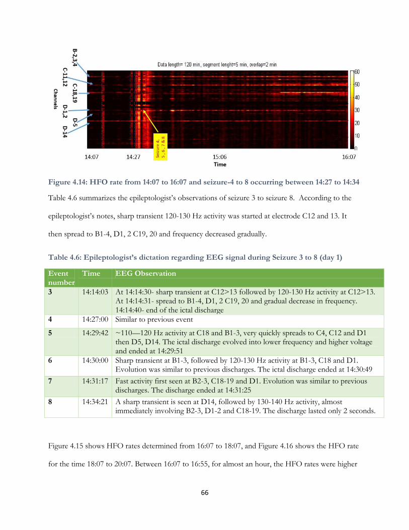
66
Figure 4.14: HFO rate from 14:07 to 16:07 and seizure-4 to 8 occurring between 14:27 to 14:34
Table 4.6 summarizes the epileptologist‘s observations of seizure 3 to seizure 8. According to the
epileptologist‘s notes, sharp transient 120-130 Hz activity was started at electrode C12 and 13. It
then spread to B1-4, D1, 2 C19, 20 and frequency decreased gradually.
Table 4.6: Epileptologist’s dictation regarding EEG signal during Seizure 3 to 8 (day 1)
Event number
Time EEG Observation
3 14:14:03 At 14:14:30- sharp transient at C12>13 followed by 120-130 Hz activity at C12>13. At 14:14:31- spread to B1-4, D1, 2 C19, 20 and gradual decrease in frequency. 14:14:40- end of the ictal discharge
4 14:27:00 Similar to previous event
5 14:29:42 ~110—120 Hz activity at C18 and B1-3, very quickly spreads to C4, C12 and D1 then D5, D14. The ictal discharge evolved into lower frequency and higher voltage and ended at 14:29:51
6 14:30:00 Sharp transient at B1-3, followed by 120-130 Hz activity at B1-3, C18 and D1. Evolution was similar to previous discharges. The ictal discharge ended at 14:30:49
7 14:31:17 Fast activity first seen at B2-3, C18-19 and D1. Evolution was similar to previous discharges. The discharge ended at 14:31:25
8 14:34:21 A sharp transient is seen at D14, followed by 130-140 Hz activity, almost immediately involving B2-3, D1-2 and C18-19. The discharge lasted only 2 seconds.
Figure 4.15 shows HFO rates determined from 16:07 to 18:07, and Figure 4.16 shows the HFO rate
for the time 18:07 to 20:07. Between 16:07 to 16:55, for almost an hour, the HFO rates were higher

67
in several channels, but considerably higher HFO rates can be observed in B-2,4, C-11,12, C-18,19,
D-1,2,3 and D-14. From 16:55 to 17:50 the seizure HFOs rate over the channels were reduced but
B-2, C-11, C-18, D-1 and D-14 continue to show higher rates. During seizure 9 at 17:51 and seizure
10 to 14 occurring between 18:00 to 18:07 HFO rates were really high across most the channels.
Figure 4.15: HFO rate over time 16:07 to 18:07 and seizure-9 occurring at 17:51 and seizure 10 to 14 occurring between 18:00 to 18:07
HFO rates were higher in most channels during 18:07 to 18:12 (Figure 4.16). It then decreased in
most channels except for the 5 electrodes B-2, C-11, 18, D-1 and D-14 which continue to show
higher rate over time although at varying rate. Approximately 25 minutes into the recording HFO
rates increased across the channels but this was not marked as a seizure event. There was a seizure
event at 19:10 but HFO rates were not high across the channels.

68
Figure 4.16: HFO rate over time 18:07 to 20:07 and seizure-15 occurring at 19:10
Table 4.7 provides the epileptologist‘s notes for seizure events 9 to 15. From the table it can
summarized that electrodes B-1, 2, 3, C-18, 19, 20, C-9, 10, 11, D-1, 2 and D13-14 electrodes are
showing fast activities which include sharp transient followed by oscillations greater than 130 Hz
and brief discharge of frequencies over 80 Hz.
Table 4.7: Epileptologist’s notes regarding EEG signal during Seizure 9 to 15 (day 1)
Event number
Time EEG Observation
9 17:51:04 120 Hz activity at C12, within 0.5 second spread to D1 and B1-3 then C19, then C25-26. The ictal discharge evolves into a lower frequency. Fast activity persists at C10-12, while rhythmic theta is seen predominantly at B1-4. C9-10, C18, C20 and D1-2.
10 18:00:00 Sharp transient at B1-3, followed by 120-130 Hz activity at B1-3, C18 and D1. Evolution was similar to previous discharges.
11 18:01:00 Onset was a sharp transient followed by >130 Hz fast activity at B1-3, C18-19, C10-11, D1-2 and D13-14.
12 18:03:04 Sharp transient at B1-3 followed by gamma activity at B1-3, C18, D1, lasting < 1 second
13 18:06:00 ~ 120 Hz activity at B1-3> C18-19>F1-2, C10-12 then D14 -- > evolution into beta activity
14 18:07:00 The jerking movement correlates to 1-2 seconds of gamma activity at B2-3, C18-19 and D1
15 19:10:00 There were recurrent brief discharges of > 80 Hz activity starting at B3-4 and lasting 5-8 seconds
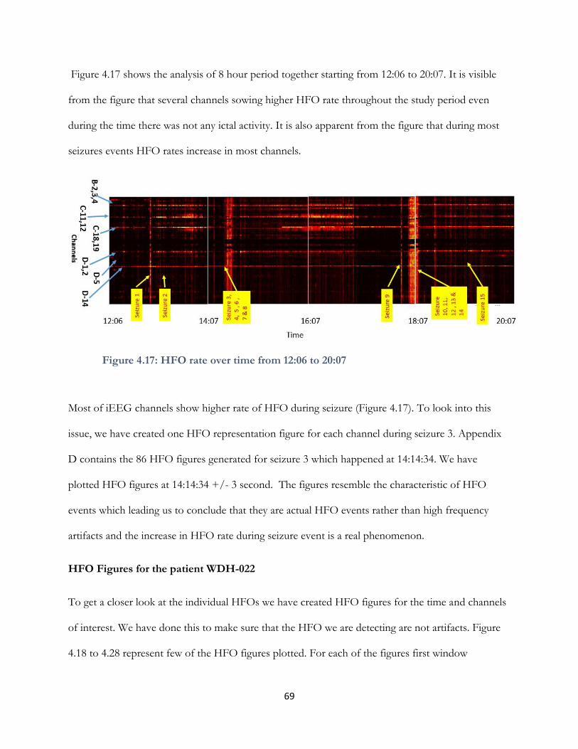
69
Figure 4.17 shows the analysis of 8 hour period together starting from 12:06 to 20:07. It is visible
from the figure that several channels sowing higher HFO rate throughout the study period even
during the time there was not any ictal activity. It is also apparent from the figure that during most
seizures events HFO rates increase in most channels.
Figure 4.17: HFO rate over time from 12:06 to 20:07
Most of iEEG channels show higher rate of HFO during seizure (Figure 4.17). To look into this
issue, we have created one HFO representation figure for each channel during seizure 3. Appendix
D contains the 86 HFO figures generated for seizure 3 which happened at 14:14:34. We have
plotted HFO figures at 14:14:34 +/- 3 second. The figures resemble the characteristic of HFO
events which leading us to conclude that they are actual HFO events rather than high frequency
artifacts and the increase in HFO rate during seizure event is a real phenomenon.
HFO Figures for the patient WDH-022
To get a closer look at the individual HFOs we have created HFO figures for the time and channels
of interest. We have done this to make sure that the HFO we are detecting are not artifacts. Figure
4.18 to 4.28 represent few of the HFO figures plotted. For each of the figures first window

70
represents a 10 s raw iEEG data around the HFO events. Second window shows 0.5 s EEG signal
and third window represent the iEEG signal after band-pass filtering. The fourth window shows the
time frequency representation of the HFO event and the last window shows the Power Spectral
Density (PSD Unit: 10log10mV2Hz-1).
Figure 4.18 shows a HFO event for the channel B-2. The approximate time of the HFO occurring is
15:03. The frequencies recorded at the peak of the EoI are, HFO peak at 106 Hz, trough at 68 Hz
and a low frequency peak at 27 Hz. So the HFO has higher power at frequencies around 106 Hz,
power gap around 68 Hz frequency and low frequency peak at 27 Hz. The time-frequency space
representation validate this.
Figure 4.19 shows a HFO event for the channel B-3, at approximately 14:26. HFO peak frequency is
106 Hz, trough at 68 Hz and a low frequency peak at 27 Hz. So the HFO has higher power at
frequencies around 112 Hz, power gap around 52 Hz frequency and low frequency peak at 40 Hz.
The time-frequency space representation shows there is an energy gap around 52 Hz frequency.
Similarly figure 420 to 4.28 shows the HFO generated in electrodes B-4, C-11, 12, C-18-19, D-1, 2, 5
and D-14. In most of these figures in the time-frequency space representation there is a high
frequency high power region and a low frequency high power region separated by a power trough.

71
Figure 4.18: HFO plotted for electrode B-2, approximate time 15:03. The frequencies recorded at the peak of the EoI are, HFO peak at 106 Hz, trough at 68 Hz and a low frequency peak at 27 Hz.

72
Figure 4.19: HFO plotted for electrode B-3, approximate time 14:26. The frequencies recorded at the peak of the EoI are, HFO peak at 112 Hz, trough at 52 Hz and a low frequency peak at 40 Hz.

73
Figure 4.20: HFO plotted for electrode B-4, approximate time 14:28. The frequencies recorded at the peak of the EoI are, HFO peak at 119 Hz, trough at 41 Hz and a low frequency peak at 28 Hz.

74
Figure 4.21: HFO plotted for electrode C-11, approximate time 14:41. The frequencies recorded at the peak of the EoI are, HFO peak at 127 Hz, trough at 85 Hz and a low frequency peak at 29 Hz.

75
Figure 4.22: HFO plotted for electrode C-12, approximate time 14:15. The frequencies recorded at the peak of the EoI are, HFO peak at 120 Hz, trough at 73 Hz and a low frequency peak at 56 Hz.

76
Figure 4.23: HFO plotted for electrode C-18, approximate time 14:15. The frequencies recorded at the peak of the EoI are, HFO peak at 136 Hz, trough at 87 Hz and a low frequency peak at 10 Hz.

77
Figure 4.24: HFO plotted for electrode C-19, approximate time 14:42. The frequencies recorded at the peak of the EoI are, HFO peak at 126 Hz, trough at 60 Hz and a low frequency peak at 28 Hz.

78
Figure 4.25: HFO plotted for electrode D-1, approximate time 14:49. The frequencies recorded at the peak of the EoI are, HFO peak at 115 Hz, trough at 64 Hz and a low frequency peak at 14 Hz.

79
Figure 4.26: HFO plotted for electrode D-2, approximate time 14:30. The frequencies recorded at the peak of the EoI are, HFO peak at 110 Hz, trough at 63 Hz and a low frequency peak at 35 Hz.

80
Figure 4.27: HFO plotted for electrode D-5, approximate time 14:19. The frequencies recorded at the peak of the EoI are, HFO peak at 111 Hz, trough at 80 Hz and a low frequency peak at 42 Hz.
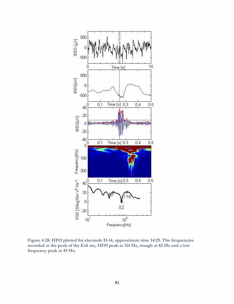
81
Figure 4.28: HFO plotted for electrode D-14, approximate time 14:29. The frequencies recorded at the peak of the EoI are, HFO peak at 114 Hz, trough at 82 Hz and a low frequency peak at 49 Hz.

82
Sensitivity of the Detection method
We have observed that the number of events of interest (and, therefore, the number of HFOs)
depends on the amplitude threshold value used in stage-1 of the detection method. For a two hour
study period we have determined the HFO rates for four different threshold values. Figure 4.29
presented these four scenarios. Some of these threshold values are quite high for detecting EoI but
we used it to check the robustness of the detection algorithm. From the figure it can be concluded
that as the threshold value increases the HFO rate decreases but the channels with higher rate
continue to show higher HFO rate compared to other channels.
Figure 4.29: HFO rate determined for 14:07 to 16:07 for different amplitude threshold value of

83
(a) Mean of all envelope + 2 x (maximum standard deviation) (b) Mean of all envelope + 3 x
(maximum standard deviation) (c) Mean of all envelope + 4 x (maximum standard deviation) (d)
Mean of all envelope + 5 x (maximum standard deviation)
4.2.2. Patient ID- SH-EEG
The second iEEG data analyzed in our study was collected during June, 2012. The information of
the patient is given in Table 4.8. One contact grid array and 10 contact strip electrodes were used to
record from 76 locations. The list of the electrodes is given in Table 4.9. The electrodes were placed
in left media, left lateral, subtemporal and superior temporal part of the brain. The diagram of the
electrode placement is provided in Appendix B.
Table 4.8: Information of the second subject of our study
Patient ID SH-EEG (subject 2)
Study Duration 6/12/2012 to 6/20/2012
Sampling Frequency 1000 Hz
Number of Channel 76
Decision about SOZ Conclusive
Table 4.9: Electrode Grids and strips used for patient - SH-EEG

84
HFO rate for all channels over a two hour time period from 19:09 to 21:09 was determined. The bar
plot in Figure 4.30 shows the channels marked with green arrow have HFO rate higher than half of
maximum rate during the two hour study. So electrodes C-34, D-39 and D-40 have higher HFO
rate. Table 5.10 shows epileptologist‘s dictation about seizure 1, 2 and 3. From the table we know
that spike wave were started at electrodes D37-42 and the following beta buzz evolved into a high-
amplitude spike pattern maximum at contacts D-39, 40, and C-34. These electrodes are pointed with
red arrow in the bar chart. The three electrodes which we found to have higher HFO rate falls
within the findings of epileptologist.
Figure 4.30: Total number of HFO detected over a 2 hours of study. The green arrow point the channels with higher HFO and the red arrow shows the channels which can be the possible SOZ.

85
Table 4.10: Epileptologist’s note about the first three seizure events (day 1)
Event number
Time EEG Observation
1 21:01:23 Repetitive spike-wave discharges (5 to 6 Hz) were noted at electrode contacts D37-42 for 1 second at 21:01:23 on 6/12/2012. This was followed by a beta buzz at 21:01:25. This evolved into a high-amplitude spike pattern maximum at contacts 39, 40, and 34. This pattern evolved, becoming higher in amplitude and slower in frequency before spontaneously terminating at 21:02:22.
2 23:47:54 Electrographically, high-amplitude repetitive spikes were noted at electrodes 40-42 and 34 at 23:47:54. This was followed by a beta buzz at 23:47:56 and then evolved into a high-amplitude spike and polyspike repetitive pattern (6 to 7 Hz) at 23:47:57. This evolved becoming higher in amplitude and slower in frequency before spontaneously terminating at 23:49:05.
3 01:49:27 Electrographically, similar ictal pattern beginning with repetitive spikes was noted at 01:49:27. This evolved with a beta buzz at 01:49:25 and then evolved into a higher amplitude with repetitive spike-wave discharge. It evolved to a higher amplitude with slower frequency before spontaneously terminating.
We determined HFO rate for 8 hour study period from 19:09 to 03:09. The result is plotted in figure
21. Three seizure events took place within this time window. According to the epileptologist‘s note
presented in Table 4.10 there wasn‘t any high frequency activity going on during the seizure events.
Figure 21 definitely confirms that. The number of HFO detected in different channels weren‘t too
high but few of the channels continuously showed higher HFO rate even when there wasn‘t any ictal
activity going on. These channels are C-34, C39, 40 and C-28. The epileptologist found C-34, C-39
and 40 as a channel of interest but not C-28.

86
Figure 4.31: HFO rate over time from 19:09 to 03:09 with 1 minute window at a time and 30 seconds overlap
Figure 4.32 to 4.35 show HFO figures in channel C-34, D-39, D-40 and C-28 chosen randomly.
For each of the figures first window represents a 10 s raw iEEG data around the HFO events.
Second window shows 0.5 s EEG signal and third window represent the iEEG signal after band-
pass filtering. The fourth window shows the time frequency representation of the HFO event and
the last window shows the Power Spectral Density (PSD Unit: 10log10mV2Hz-1). These figures
show higher energy at the high frequency peak and low frequency peak separated by an energy gap
at the trough frequency.

87
Figure 4.32 : HFO plotted for electrode C-34, approximate time 20:50. The frequencies recorded at the peak of the EoI are, HFO peak at 94 Hz, trough at 40 Hz and a low frequency peak at 28 Hz.

88
Figure 4.33: HFO plotted for electrode D-39, approximate time 19:49. The frequencies recorded at the peak of the EoI are, HFO peak at 96 Hz, trough at 42 Hz and a low frequency peak at 22 Hz.

89
Figure 4.34: HFO plotted for electrode D-40, approximate time 19:41. The frequencies recorded at the peak of the EoI are, HFO peak at 100 Hz, trough at 60 Hz and a low frequency peak at 39 Hz.

90
Figure 4.35: HFO plotted for electrode C-28, approximate time 19:26. The frequencies recorded at
the peak of the EoI are, HFO peak at 102 Hz, trough at 47 Hz and a low frequency peak at 39 Hz.
The results (Figure 4.10 & 4.30) from analyzing the iEEG data obtained from EMU show that,
channels with high HFO rate corresponds to the channels the epileptologist found to be the seizure
onset zone. The heat maps of HFO rate determined over time provide interesting insight about how
HFO rate changes over time. Even when the patient is not having any seizure the HFO rate tend to
stay high in certain channels and these channels are also described to be the possible focal point by
the epileptologist. Another point to note from these heat maps is during most seizures HFO rate
tend to be high in most channels. We have also provided some HFO representative figures chosen
randomly in the channels where HFO rate is high. These HFO figures have the similar
characteristics of the HFO presented by Burnos, et. al. [5].

91
5. Discussion
The goal of this thesis was to validate the HFO detection algorithm proposed by Burnos, et. al. [5],
modify it to apply on EMU data, and to compare the findings with the epileptologist‘s notes with
the goal of establishing a relationship between the regions exhibiting higher HFO rates and the SOZ
identified by the epileptologist. We have successfully validated the detection algorithm using a data
sample obtained from the author [5] and also by using a simulated HFO that we created. We have
modified the algorithm to apply to the EMU data and found that the electrode sites producing
HFOs at higher rates are also the ones the epileptologist found to comprise the SOZ. We have also
noticed that these electrodes continue to show higher HFO rates for the entire duration of study.
The algorithm as implemented in Matlab for this thesis was able to detect the 7 HFOs (Table 4.1) in
a data sample provided by the author. The HFO characteristic showed in Figure 4.2 also matches
with the one presented by the author (Figure 4.2). The HFO detection algorithm developed by
Burnos, et. al. [5] was successfully validated.
We have taken the HFO characteristics from the literature [5, 8, & 30] and created a prototypical
oscillation (Figure 4.4) that simulates an HFO. Equation 1 (Methodology) was used to create the
formula. Then we inserted this synthetically created HFO into a section of the example data (Figure
4.5). The HFO detection algorithm detected 8 events this time and the frequency, time and
amplitude (Table 4.2) of the newly detected event matches the simulated event we created. The
HFO representation (Figure 4.8) also confirms this fact, thereby verifying that the HFO detection
algorithm we implemented is actually detecting HFO events.
Then we modified the algorithm to work with the EMU data. The two patient‘s iEEG data used in
this purpose were both sampled at 1000 Hz. Two hour iEEG data for the first patient (WDH-022)

92
recorded from 14:07 to 16:07 on 10/22/2014 was analyzed to determine total number of HFOs.
The iEEG channels having higher numbers of HFO event were compared with the finding of the
epileptologist (Figure 4.10). The electrodes with higher HFO rates (B4, C12, C18, D1 and D14) are
within the electrodes that the epileptologist found to be in the onset zone of the seizure. The HFO
analysis method provides a refinement of the SOZ identified be the epileptologist. So it allows the
epileptologist to focus on a smaller set of channels than those he/she initially identified through
visual inspection. This fact leads us to believe that HFOs have potential to be a biomarker for
identifying sites prone to be involved in seizure activity.
In the results section Figures 4.11 to 4.17 show how HFO rate changes over time for an 8 hour time
duration. The analysis was done two hours at a time and finally merged in Figure 4.17. We have
noticed a significantly higher number of HFOs present at all recording sites during some seizure
events. The interesting phenomenon to notice in these figures is the continuously higher HFO rate
in few of the electrodes (B-2, 4, C-11, 12, D1, D-5, 14) even if there is not seizure present at that
time. HFO rate in these channels stayed comparatively high for the entire 8 hour duration thus
suggesting that the rate of HFO may not be a good predictor of seizure onset (Figure 4.17). To look
closely into these channels and make sure the events we are detecting are actually HFOs, we have
plotted randomly chosen HFO events in these channels (B-2, 3, 4, C-11, 12, D-1, 2, 5, 14). These
events are presented in Figure 4.18 to 4.28. The HFO figures matches with the characteristics of
HFOs. So the electrodes with higher rate are actually caused by presence of more frequent HFO
events. This may indicate that using a HFO detection method can assist in locating the SOZ by
analyzing any time period of the study, even prior to the occurrence of a seizure.
During some seizure endured by Patient WDH-022, we have noticed an increment of HFO rates
across most of the channels (Figure 4.17). To investigate this issue further we have plotted HFO

93
figures (Appendix D) for all the channels at the onset of seizure 3 (14:14:34). We have found the
charecteristics of the figures to be similar to HFO events. This made us believe that the increment
of HFO rates during some seizure events is not due to high frequency artifacts.
The other iEEG data (Patient ID: SH-EEG) we have analyzed was recorded in 6/12/2012. Like the
previous patient we have determined total HFO for a two hour study period. The channels with
higher HFO rate (C-34, D-39 & D-40) were plotted in Figure 4.30 along with the electrodes
epileptologist marked to be the SOZ (C-34, D-37 to 42). Similar to the previous patient the
electrodes showing higher HFO rate are also the electrodes epileptologist‘s found to be in the onset
zone of the seizure but not all channels in the seizure onset zone had significantly high HFO count.
We have also randomly plotted few HFO events in these channels (Figure 4.32 to 4.35 to confirm
that the detected events appear to have the characteristics of a HFO. We also determined how HFO
rate changes over an 8 hour period of time (Figure 4.31). Although the HFO rates were much lower
for this patient few of the electrodes (C-34, D-39 & D-40) consistently showed higher HFO rate.
These confirm the findings from the last patient. HFOs are more like to be generated in the SOZ
and HFO area can be determined analyzing any part of the study.
The number of HFOs varies significantly depending on the threshold set in stage 1 of the HFO
detection algorithm. We have varied the threshold and calculated how HFO rates changes over time
(Figure 4.29). Although the HFO rates drop significantly with the threshold increment but the
electrodes with higher HFO rates still continue to show comparatively higher HFO rate than
background. So changing the threshold is not likely to change the relative frequency of occurrence
of HFOs in signals associated with the SOZ compared with other iEEG signals outside of the SOZ.
The recommended threshold is determined using the mean envelope and three times the
corresponding standard over all channels, not just a particular channel.

94
The HFO detection method introduced in this research is organized as a MATLAB tool called HFO
Analysis Tool (Appendix C), which can be used to see how HFO rate is changing over time, which
channels are generating more HFOs and then create HFO characteristic figures for a particular
channel and time window. The analysis performed by this tool can provide insight about the SOZ
from a HFO perspective. This will help the neurosurgon augment information about the epileptic
zone and make a better surgical decision.

95
6. Future work
The logical next step of this research would be to get post-surgical information to assess the success
of the surgery. After comparing the area of the brain that was surgically removed and HFO region
we determined, we can decide the how HFO region compares with epileptic zone. Also analyzing
additional data will help to build more confident on our study.
A HFO Analysis Tool (Appendix C) combines HFO detection with a visualization procedure that
can identify HFOs in segments of the recorded iEEG. The epileptologist will then be able to use the
tool while conducting an intracranial EEG study to focus on events in a recorded channel at a
specific time. This will tell the epileptologist which channels are generating more HFO and can help
identify the possible SOZ.
Some studies [6, 9, 31] claimed fast ripples (250 -500 Hz) [8] are associated more closely with the
epileptic zone. In future the unsupervised HFO classification method presented by Blanco, et. al. [4]
can be implemented to classify HFOs into ripples (100-250 Hz) [8], fast ripples and mixed frequency
events. To look at fast ripples the sampling frequency should be set at 2000 Hz and the anti-aliasing
filter should be set at higher than 500 Hz.
In this study we focused mainly on HFO detection and rate. Future work on HFOs can be focusing
more on the characteristics of HFO (frequency, time duration, amplitude, power) and how they
change before and after seizure. If these features are found to be related to a following seizure, an
appropriate statistical analysis might be utilized to predict seizure. This will help seizure interrupting
devices to predict seizure before its onset and interrupt it.

96
7. Conclusion
This thesis contributes to epilepsy diagnosis by introducing the HFO measure in pre-surgical iEEG
monitoring. After successfully validating and verifying the HFO detection algorithm we have
modified it and applied it on EMU data. After comparing our findings with the epileptologist‘s
analysis we found that HFO region falls within the SOZ and smaller. This may aid the surgeon in
delineating a potential epileptogenic zone and maybe reduce the resection size.
We have also found that HFO rates remain comparatively high in the HFO region for the entire
duration of the study. This phenomenon was observed for both of the patients and introduces a
possibility that a decision about the SOZ can be guided by analyzing a short duration of the study
for HFO. This could significantly reduce the duration for invasive video electroencephalographic
monitoring epilepsy patients have to go through.
The HFO Analysis Tool (Appendix C) can be used the epileptologist to perform the analysis
presented in this thesis. The entire analysis can be done in reasonably short time (3 to 4 hours),
which give the epileptologist to use the tool while a patient is being monitored with invasive EEG.
Although additional work is required including analyzing more patient‘s data, comparing with post-
surgical outcome but this research investigates the applicability of HFO in clinical epilepsy diagnosis.
With further work this may lead to better SOZ delineation and significantly reduce the iEEG
monitoring duration, which could lead to better surgical outcome for resection surgery or better
performance of seizure interruption devices.

97
8. Bibliography
[1] M. J. Brodie, S. C. Schachter, and P. Kwan, ―Fast Facts : Epilepsy,‖ 2012. http://doi.org/10.3233/PEP-13043 [2] Begley, C. E., M. Famulari, J. F. Annegers, D. R. Lairson, T. F. Reynolds, S. Coan, & W. A. Rocca. (2000). The cost of epilepsy in the United States: an estimate from Population- based clinical and survey data. Epilepsia, 41(3), 342-351. [3] W. Stacey, M. Le Van Quyen, F. Mormann, and A. Schulze-Bonhage, ―What is the present-day
EEG evidence for a preictal state?,‖ Epilepsy Res., vol. 97, no. 3, pp. 243–51, Dec. 2011. [4] J. a Blanco, ―Unsupervised Classification of High-Frequency Oscillations in neocortical
Epilepsy and Control Patients,‖ p. 158, 2010. [5] S. Burnos, P. Hilfiker, O. Sürücü, F. Scholkmann, N. Krayenbühl, T. Grunwald, and J.
Sarnthein, ―Human intracranial high frequency oscillations (HFOs) detected by automatic time-frequency analysis,‖ PLoS One, vol. 9, no. 4, 2014.
[6] A. Bragin, I. Mody, C. L. Wilson, and J. Engel, ―Local generation of fast ripples in epileptic
brain.,‖ J. Neurosci., vol. 22, no. 5, pp. 2012–2021, 2002. [7]A. Bragin, C. L. Wilson, J. Almajano, I. Mody, and J. Engel, ―High-frequency oscillations after
status epilepticus: Epileptogenesis and seizure genesis,‖ Epilepsia, vol. 45, no. 9, pp. 1017–1023, 2004.
[8] A. Pearce, D. Wulsin, J. A. Blanco, A. Krieger, B. Litt, and W. C. Stacey, ―Temporal changes of neocortical high-frequency oscillations in epilepsy.,‖ J. Neurophysiol., vol. 110, no. 5, pp. 1167–79, Sep. 2013.
[9] G. Birot, A. Kachenoura, L. Albera, C. Bénar, and F. Wendling, ―Automatic detection of fast ripples,‖ J. Neurosci. Methods, vol. 213, no. 2, pp. 236–249, 2013.
[10]R. G. Stockwell Why use the S-transform. AMS Pseudo-differential operators: Partial differential equations and time-frequency analysis 52: 279– 309, 2007
[11]B. Crépon, V. Navarro, D. Hasboun, S. Clemenceau, J. Martinerie, M. Baulac, C. Adam, and M. Le Van Quyen, ―Mapping interictal oscillations greater than 200 Hz recorded with intracranial macroelectrodes in human epilepsy,‖ Brain, vol. 133, no. 1, pp. 33–45, 2010.
[12]Food and Drug Administration. Rns ® System for Epilepsy Sponsor Executive Summary.
2013, Retrieved on: 8/3/2015 Website: http://www.fda.gov/downloads/AdvisoryCommittees/CommitteesMeeting

98
Materials/MedicalDevices/MedicalDevicesAdvisoryCommittee/ NeurologicalDevicesPanel/UCM340257.pdf
[13]NIHON KOHDEN, EEG Systems/Neurofax, Retrieved on: 8/3/2015 Website: http://www.nihonkohden.de/products/neurology/eeg/epilepsy/eeg-
1200.html?L=1 [14]M. J. England, C. T. Liverman, A. M. Schultz, and L. M. Strawbridge, ―Epilepsy across the
spectrum: Promoting health and understanding. A summary of the Institute of Medicine report,‖ Epilepsy Behav., vol. 25, no. 2, pp. 266–276, 2012.
[15] A. Lozano, P. Gildenberg and R. Tasker, Textbook of stereotactic and functional neurosurgery. Berlin:
Springer, 2009.
[16] C. Haegelen, P. Perucca, C. E. Châtillon, L. Andrade-Valença, R. Zelmann, J. Jacobs, D. L. Collins, F. Dubeau, A. Olivier, and J. Gotman, ―High-frequency oscillations, extent of surgical resection, and surgical outcome in drug-resistant focal epilepsy,‖ Epilepsia, vol. 54, no. 5, pp. 848–857, 2013..
[17] L. P. Andrade-Valenca, F. Dubeau, F. Mari, R. Zelmann, and J. Gotman, ―Interictal scalp fast oscillations as a marker of the seizure onset zone,‖ Neurology, vol. 77, no. 6, pp. 524–531, 2011.
[18] J. a Blanco, ―Unsupervised Classification of High-Frequency Oscillations in neocortical Epilepsy and Control Patients,‖ p. 158, 2010.
[19] J. O‘Keefe, ―Place units in the hippocampus of the freely moving rat.,‖ Exp. Neurol., vol. 51, no. 1, pp. 78–109, 1976.
[20] Buzsaki, G. High-frequency network oscillation in the hippocampus. Science 256, 1025{1027, 1992.
[21] G. Buzsáki, L. Leung, and C. Vanderwolf, ―Cellular bases of hippocampal EEG in the behaving rat,‖ Brain Research, vol. 287, no. 2, pp. 139–171, 1983.
[22]Ylinen, A., Bragin, A., Nadasdy, Z., Jando, G., Szabo, I., Sik, A., and Buzsaki, G. Sharp wave-associated high-frequency oscillation (200 Hz) in the intact hippocampus: Network and intracellular mechanisms. The Journal of Neuroscience 15, 1, 30{46. 144, 1995.
[23]Draguhn, A., Traub, R. D., Schmitz, D., and Jefferys, J. G. R. Electrical coupling underlies high-frequency oscillations in the hippocampus in vitro. Nature 394 , 189{192, 1998
[24] A. Bragin, J. Engel, C. L. Wilson, I. Fried, and G. Buzsáki, ―High-frequency oscillations in human brain.,‖ Hippocampus, vol. 9, no. 2, pp. 137–42, Jan. 1999.
[25]Wilson, M. A., and B. L. McNaughton, Reactivation of hippocampal ensemble memories during sleep. Science 265, 676{679, 1994.
[26] F. Grenier, I. Timofeev, and M. Steriade, ―Focal Synchronization of Ripples (80-200 Hz) in Neocortex and Their Neuronal Correlates,‖ J Neurophysiol, vol. 86, no. 4, pp. 1884–1898, Oct. 2001.

99
[27]Buzsaki G, Z, Horvath, R, Urioste, J, Hetke, K, Wise, High-frequency network oscillation in the hippocampus. Science. 256:1025–1027, 1992 [PubMed: 1589772]
[28] M. A. Howard, I. O. Volkov, M. D. Noh, M. A. Granner, R. Mirsky, and P. C. Garell, ―Chronic microelectrode investigations of normal human brain physiology using a hybrid depth electrode.,‖ Stereotact. Funct. Neurosurg., vol. 68, no. 1–4 Pt 1, pp. 236–42, Jan. 1997.
[29] J. Jacobs, M. Zijlmans, R. Zelmann, C.-E. Chatillon, J. Hall, A. Olivier, F. Dubeau, and J. Gotman, ―High-frequency electroencephalographic oscillations correlate with outcome of epilepsy surgery.,‖ Ann. Neurol., vol. 67, no. 2, pp. 209–20, Feb. 2010.
[30] J. Jacobs, R. Zelmann, J. Jirsch, R. Chander, C.-E. C. F. Dubeau, and J. Gotman, ―High frequency oscillations (80-500 Hz) in the preictal period in patients with focal seizures.,‖ Epilepsia, vol. 50, no. 7, pp. 1780–92, Jul. 2009.
[31] T. Akiyama, B. McCoy, C. Y. Go, A. Ochi, I. M. Elliott, M. Akiyama, E. J. Donner, S. K. Weiss, O. C. Snead, J. T. Rutka, J. M. Drake, and H. Otsubo, ―Focal resection of fast ripples on extraoperative intracranial EEG improves seizure outcome in pediatric epilepsy.,‖ Epilepsia, vol. 52, no. 10, pp. 1802–11, Oct. 2011.
[32] K. Jerbi, T. Ossandón, C. M. Hamamé, S. Senova, S. S. Dalal, J. Jung, L. Minotti, O. Bertrand, A. Berthoz, P. Kahane, and J.-P. Lachaux, ―Task-related gamma-band dynamics from an intracerebral perspective: review and implications for surface EEG and MEG.,‖ Hum. Brain Mapp., vol. 30, no. 6, pp. 1758–71, Jun. 2009.
[33] Bartolomei F, M, Guye , M, Gavaret, J, Regis, F, Wendling, C, Raybaud et al. The presurgical evaluation of epilepsies. Rev Neurol (Paris)158:4S55–64S, 2002.
[34] Bossemeyer, R., EGR-534, Biolectric Potential, Class Lecture-Brain and EEG, Fall-2014
[35] [1] Mayo Clinic Staff, 'Symptoms and causes - Epilepsy - Mayo Clinic', Mayoclinic.org, 2015. [Online]. Available: http://www.mayoclinic.org/diseases-conditions/epilepsy/symptoms-causes/dxc-20117207. [Accessed: 04- Aug- 2015].
[36] P. van Mierlo, E. Carrette, H. Hallez, K. Vonck, D. Van Roost, P. Boon, and S. Staelens,
―Accurate epileptogenic focus localization through time-variant functional connectivity analysis of intracranial electroencephalographic signals.,‖ Neuroimage, vol. 56, no. 3, pp. 1122–33, Jun. 2011.
[37] P. O. Shafer, 'About Epilepsy: The Basics', Epilepsy Foundation, 2015. [Online]. Available: http://www.epilepsy.com/learn/about-epilepsy-basics. [Accessed: 04- Aug- 2015].
[38] Shah AK, Mittal S. Invasive electroencephalography monitoring: Indications and presurgical planning. Ann Indian Acad Neurol, 17, Suppl S1:89-94, 2014.
[39] A. I. Yang, X. Wang, W. K. Doyle, E. Halgren, C. Carlson, T. L. Belcher, S. S. Cash, O. Devinsky, and T. Thesen, ―Localization of dense intracranial electrode arrays using magnetic resonance imaging,‖ Neuroimage, vol. 63, no. 1, pp. 157–165, 2012.

100
[40] Shop.inomed.com, 'inomed | Grid/Strip Electrodes 8 Strips | 8 Contacts | Medical Devices', 2015. [Online]. Available: https://shop.inomed.com/Grid-Strip-Electrodes-8-Strips-8-Contacts.html. [Accessed: 04- Aug- 2015].
[41] Diximedical.net, 'Dixi Medical » Intracerebral electrodes', 2015. [Online]. Available: http://www.diximedical.net/GB/?cat=24. [Accessed: 04- Aug- 2015].
[42] Biomed.brown.edu, 'High Tech Prosthetics - Neural Prosthetics - Emerging Technology', 2015. [Online]. Available: http://biomed.brown.edu/Courses/BI108/2006-108websites/group07HighTechProsthetics/pages/neurotech.htm. [Accessed: 04- Aug- 2015].
[43]Kesavadas C, B. Thomas, Clinical applications of functional MRI in epilepsy. The Indian Journal of Radiology & Imaging.18(3):210-217. doi:10.4103/0971-3026.41829, 2008.
[44]R. D Sheth and S. R Benbadis, 'EEG in Common Epilepsy Syndromes: Role of EEG in Epilepsy Syndromes, Neonatal Seizures, Infantile Spasms and West Syndrome', Emedicine.medscape.com, 2015. [Online]. Available: http://emedicine.medscape.com/article/1138154-overview. [Accessed: 04- Aug- 2015].
[45] S. Ramon y Cajal, Histologie du systeme nerveux de l'homme et des vertebres. Paris: Maloine, 1911.
[46] H. Gray and W. Lewis, Anatomy of the human body. Philadelphia: Lea & Febiger, 1918.
[47] LeDoux, J.E. Emotion, memory and the brain. Scientific American; 270:50-57, 1994.
[48] Elisevich, K. Study of Imaging, Electrographic Signal Characteristics, and Neurobiological Features in Focal Epilepsy, Department of Clinical Neurosciences, Spectrum Health System, Version 5.
[49] R. J. Staba, C. L. Wilson, A. Bragin, I. Fried, and J. J. Engel, ―Quantitative Analysis of High-Frequency Oscillations (80-500 Hz) Recorded in Human Epileptic Hippocampus and Entorhinal Cortex,‖ J Neurophysiol, vol. 88, no. 4, pp. 1743–1752, Oct. 2002.
[50] B. Crépon, V. Navarro, D. Hasboun, S. Clemenceau, J. Martinerie, M. Baulac, C. Adam, and M. Le Van Quyen, ―Mapping interictal oscillations greater than 200 Hz recorded with intracranial macroelectrodes in human epilepsy.,‖ Brain, vol. 133, no. Pt 1, pp. 33–45, Jan. 2010.
[51] H. Otsubo, A. Ochi, K. Imai, T. Akiyama, A. Fujimoto, C. Go, P. Dirks, and E. J. Donner, ―High-frequency oscillations of ictal muscle activity and epileptogenic discharges on intracranial EEG in a temporal lobe epilepsy patient.,‖ Clin. Neurophysiol., vol. 119, no. 4, pp. 862–8, Apr. 2008.
[52] M. Zijlmans, P. Jiruska, R. Zelmann, F. S. S. Leijten, J. G. R. Jefferys, and J. Gotman, ―High-
frequency oscillations as a new biomarker in epilepsy.,‖ Ann. Neurol., vol. 71, no. 2, pp. 169–78, Feb. 2012.
[53] B. Crépon, V. Navarro, D. Hasboun, S. Clemenceau, J. Martinerie, M. Baulac, C. Adam, and M. Le Van Quyen, ―Mapping interictal oscillations greater than 200 Hz recorded with intracranial macroelectrodes in human epilepsy,‖ Brain, vol. 133, no. 1, pp. 33–45, 2010.

101
[54] J. R. Cho, E. Y. Joo, D. L. Koo, S. C. Hong, and S. B. Hong, ―Clinical utility of interictal high-frequency oscillations recorded with subdural macroelectrodes in partial epilepsy.,‖ J. Clin. Neurol., vol. 8, no. 1, pp. 22–34, Mar. 2012.
[55] H. O. Lüders, I. Najm, D. Nair, P. Widdess-Walsh, and W. Bingman, ―The epileptogenic zone: General principles,‖ Epileptic Disord., vol. 8, no. SUPPL. 2, pp. 1–9, 2006.
[56] R. G. Stockwell, L. Mansinha, and R. P. Lowe, ―Localization of the complex spectrum: The S transform,‖ IEEE Trans. Signal Process., vol. 44, no. 4, pp. 998–1001, 1996.
[57] M. Javidan, ―Electroencephalography in Mesial Temporal Lobe Epilepsy: A Review,‖ Epilepsy Res. Treat., vol. 2012, pp. 1–17, 2012.
[58] Wang, Y., The Tutorial: S Transform, National Taiwan University, Taipei, Taiwan, ROC
[59] L. Schuh and I. Drury, 'Intraoperative electrocorticography and direct cortical electrical stimulation', Seminars in Anesthesia, Perioperative Medicine and Pain, vol. 16, no. 1, pp. 46-55, 1997.

102
9. Appendices
9.1. Appendix A: Clinical Events and EEG Correlation for Patient WDH-022
The following table is collected from the epileptologist‘s note on the seizure events of patient
WDH-022. It describes the time of the seizure, clinical manifestation and EEG observation. HFO
analysis performed in this thesis was compared with this note.
103

104

105

106

107

108
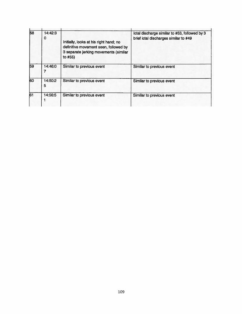
109

110
9.2. Appendix B: Electrode Locations for Patient – SH-EEG

111
Table B1: Electrode Grids

112
Clinical Events and EEG Correlation for Patient SH-EEG
6/12/12 Seizure #1. Repetitive spike-wave discharges (5 to 6 Hz) were noted at electrode contacts D37-42
for 1 second at 21:01:23 on 6/12/2012. This was followed by an electrodecrement/beta buzz at
21:01:25. This evolved into a high-amplitude spike pattern maximum at contacts 39, 40, and 34. This
pattern evolved, becoming higher in amplitude and slower in frequency before spontaneously
terminating at 21:02:22.
Clinically, the patient did not show any significant changes when he was tested by nursing personnel
at 21:02:30. He informed the nurse that he was doing okay.
Seizure #2. Electrographically, high-amplitude repetitive spikes were noted at electrodes 40-42 and
34 at 23:47:54. This was followed by an electrodecrement/beta buzz at 23:47:56 and then evolved
into a high-amplitude spike and polyspike repetitive pattern (6 to 7 Hz) at 23:47:57. This evolved
becoming higher in amplitude and slower in frequency before spontaneously terminating at 23:49:05.
Clinically, the patient was not noted to demonstrate any changes nor did he inform nursing of any
change in feeling.
Seizure #3. Electrographically, similar ictal pattern beginning with repetitive spikes was noted at
01:49:27. This evolved with an electrodecrement/beta buzz at 01:49:25 and then evolved into a
higher amplitude with repetitive spike-wave discharge. It evolved to a higher amplitude with slower
frequency before spontaneously terminating.
No clinical changes were noted.
Seizure #4. Electrographically, a repetitive spike pattern was noted over the left mesiotemporal
surface at 05:02:21, similar to the 3 previous subclinical electrographic seizures. This, again, evolved
over approximately 1 minute before spontaneously terminating.
No definitive clinical changes were noted.
6/13/12
Seizure #5: Electrographically repetitive spikes were noted at 07:33:19 at electrodes 38-42 and
electrodes 34 and 45. This was followed by an attenuation/beta buzz at 07:33:20 followed by an ictal
evolving pattern becoming higher in amplitude and slower in frequency before terminating at
7:35:35.

113
Clinically, the patient was sleeping during the event and was noted to readjust in bed at 07:34:03.
There was some rearrangement of sheets and movement of his legs, and then he appears to look to
the left. It was not clear that these were definitive ictal movements, or just typical movements during
a subclinical event.
Seizure #6 occurred at 6/13/2012 at 16:23:20. Electrographically, there was a subtle ictal pattern
involving electrode contacts 2 through 6 on A grid over the left frontal head region. This was a
subtle pattern and no clinical changes were noted during this event.
Seizure #7: Electrographically, at 16:47:57 on 6/13/2012 there was rhythmic sharply contoured
theta activity over the left frontal grid (electrodes 2 through 6), which evolved into a spike
configuration. This ictal pattern showed a subtle evolution before stopping at 16:49:24.
Clinically, no clinical changes were noted on review of the video files.
Seizure #8: Electrographically, a rhythmic, sharply contoured theta pattern was noted over the left
frontal grid at 17:04:36. This evolved similar to seizure #7, evolving to a spike-like configuration
before spontaneously terminating at 17:05:36. There appeared to be a field involving electrode 62,
which was over the right basal frontal area.
Clinically, no definitive changes were noted in the patient's behavior.
Seizure #9: Electrographically, at 22:13:44 on 6/13/2012, a beta buzz was noted. Within 2 seconds,
this evolved to a 4-6 Hz spike-like pattern, maximum at electrodes 40-42. This evolved, becoming
higher amplitude and slower in frequency before spontaneously terminating at 22:14:45.
Clinically, the patient was sleeping and at 22:14:22 he was noted to move and reached out with his
left hand. When tested by nursing personnel, he seemed to answer questions appropriately.
Seizure #10: Electrographically, at 00:05:14 on 6/14/2012, a beta buzz was noted. This evolved into
repetitive 4 Hz spike-wave pattern involving electrodes 36, 42, and 44. This subsequently showed
propagation and diffuse slowing over the frontal head regions, including the left frontal grid and the
left interhemispheric strip. This spontaneously terminated at 00:07:26.
Clinically, the patient was awake and looking around at 00:06:53. He appeared to have difficulty
answering questions, implying he could not say what he wanted to. When he was formally tested by

114
nursing personnel, there were specific questions that he could not answer, including his brother's
name at 00:07:24.
06/14/2012
Seizure #11: Electrographically, a beta buzz was identified at 21:56:45 involving electrode contacts
33-34 and 35-42. This evolved into a higher amplitude of 4-5 Hz spike and spike-wave pattern.
Initially, this became a higher amplitude and slower frequency before spontaneously terminated at
21:57:54.
Clinically, the patient was sleeping, but awakened by nursing personnel and tested. There were no
obvious changes noted during this ictal event.
Seizure #12: Electrographically at 08:24:22 on 6/16/2012, a repetitive spike discharge was noted at
08:24:22, maximum at electrode contacts 34 and 41. This changed into a beta buzz at 08:24:25 and
then evolved into a higher amplitude repetitive spike pattern initially in the theta range. This evolved
becoming higher in amplitude and slower in frequency before spontaneously terminating at
08:25:35.
Clinically no obvious clinical changes were noted during this study. The patient was sleeping and did
have movement at the end of the actual seizure.
Ictal activity: There were 2 seizures recorded during this monitoring session, 1 subclinical (seizure
#13) and 1 clinical (seizure #14).
Electrographically, at 05:26:06 on 06/17/2012, a beta buzz was recorded over electrode contacts 34
and 40. This evolved with subsequent spread to the frontal head regions at 05:26:50. This showed a
similar electrographic evolution as previously noted in both subclinical events. This spontaneously
terminated at 05:30:50.
Clinically, the patient was awake and looking around. It was noted at 05:28:07, he readjusted in the
bed and was noted to rearrange his sheets at 05:30:19. There was no formal testing with this event.
Seizure #14 on 06/17/2012. Electrographically, a beta buzz was noted at electrodes 34 and 40 at
08:16:14. This evolved similar to previous documented ictal patterns. It showed spread to the
frontal head regions at 08:16:54 and then secondary generalization at 08:24:06.
Clinically, the patient was initially sleeping with eye covers on when at 08:17:50 he was noted to
readjust his covers. At 08:18:13, the nurse was in the room testing and the patient looked confused.
He had a prolonged, blank stare. At 08:21:15, he sits up in bed and he continued to appear

115
confused. At 8:22:14, a nurse was questioning of him. At 8:24:19, these secondary generalized and
had forced contraction to the right. After the seizure, the patient was confused and combative.
Seizure #15: Electrographically at 09:13:15 on 6/17/2012, repetitive spikes were noted at contacts
34 and 40. This evolved into a beta buzz at 09:13:21. This evolved, becoming higher amplitude and
slower in frequency before terminating at 09:15:47.
Clinically, no definitive clinical changes were identified during the seizure and there was some testing
completed at 09:14:14.

116
9.3. Appendix C: HFO Analysis Tool
9.3.1. Operating Manual:
Step 1 Analysis: Determining HFO rate over time for a certain edf file
Open the file ―HFO_rate_over_time.m” and run it. The script will ask for following input
Enter link of the directory link the edf file is in :
An example directory link: C:\eegData\Riazul\Figure_1_generation\second_attempt\synthetic_sample_30_second\HFO_figure_generation_WDH\Tool
Enter the name of the .edf file (e.g. BA2681LD_1-1.edf )
Sampling Frequency (Hz) =
(e.g. 1000,2000 )
The script will open the .edf file and convert it to .mat file and analyze it for determining HFO rate for the entire file for duration 1 minute at a time with 30 seconds overlap. These two durations can be varied inside the script. Running the script might take 3 to 4 hours.
Outputs: The script will create three figures and will also save them in the current directory. The three figures are,
Total HFO Bar plot for.jpg : Plots the total HFO calculated on all EEG channels
Channels with higher HFO rate.jpg : Plots the channels which have higher HFO (>50%)
HFO Rate Heat Map.jpg : Plots HFO rate for the entire file for duration 1 minute at a time with 30 seconds overlap
The script also creates following two matrix and save them as matrix file (.mat) in the current directory,
HFO_rate_over_time.mat : HFO rate for the entire file for duration 1 minute at a time with 30 seconds overlap
HFOs_all.mat : Total HFO rate determined over entire duration of the file (usually 2 hours)
Step 2 Analysis: To create HFO figure for a particular channel and time window open the file “HFO_figure_generator.m”. Once run the script will ask for following inputs,
(1) Sampling Frequency (Hz) =
(2) The script will then show all the active channels in the particular

117
edf file. The script will ask you to name the channel you want to
select.
Enter the name of the channel you want to plot HFO for :
The script will then show the start and end of recording for the file
For example: Time recording started:14.07.02
Time recording ended:16.07.02
The script will ask you to enter the start time for the duration you want to plot HFO for with the following message.
Enter your start time (within the duration of the file) Hour(24):
Enter your start time Minute :
Enter your start time: Second :
After that it will prompt you to enter the end time of your time window.
Enter end time Hour(24):
Enter end time Minute :
Enter end time Second :
The script will then create a folder named ―output HFO Figures‖ and save the HFO figures in it.

118
9.3.2. MATLAB Scripts
HFO Rate over Time:
close all
%%%%%%%%%%%%%%%%%%%%%%%%%%%%%%%%%%%%%%%%%%%%%%%%%%%%%%%%%%%%%%%%%%%%%%%%%%%%%%%%%%%%%%%%%%%%%%%%%%%%%%%%%
% This script calculates HFO rate over time using the modified algorithm
% of Burnos, et. al. [5].
% HFO rate is calculated for smaller time window and certain overlap
% For this script, Time window=1 minute and overlap=30 seconds
% The values can be changed inside the script
% The script will ask for following inputs
% (1) link of the directory link the edf file is in :
% An example directory link:
C:\eegData\Riazul\Figure_1_generation\second_attempt\synthetic_sample_30_second\HFO_figure_generation_WDH\Tool
% (2) The name of the .edf file (e.g. BA2681LD_1-1.edf )
% (3) Sampling Frequency (Hz) =
% (e.g. 1000,2000 )
% The script will create three figures and will also save them in the current directory.
% (1)Total HFO Bar plot for.jpg
% (2)Channels with higher HFO rate.jpg
% (3)HFO Rate Heat Map.jpg
% Riazul Islam created: 6/1/2015
% Last updated: 8/5/2015
%%%%%%%%%%%%%%%%%%%%%%%%%%%%%%%%%%%%%%%%%%%%%%%%%%%%%%%%%%%%%%%%%%%%%%%%%%%%%%%%%%%%%%%%%%%%%%%%%%%%%%
disp('******** THIS SCRIPT WILL CREATE THE HEATMAP OF HFO RATE FOR A EDF FILE*********')
disp('Might take 3-4 hours to run the file')
p1='Enter link of the directory link the edf file is in :';
directory=input(p1,'s');
p1='Enter the name of the edf file (e.g. BA2681LD_1-1.edf ):';
name=input(p1,'s');
% getting the directory of the script to add the Functions path in the
% current directory
[folder, name, ext] = fileparts(which('HFO_rate_over_time'));
addpath(genpath(strcat(folder,'\Functions')));
% Sampling frequency
p1='Sampling Frequency (Hz) =';
Fs=input(p1);
[hdr, record]=edfread(strcat(directory,'\',name));
disp('Date of the edf file recorded:')
disp(hdr.startdate)
disp('Time of the edf file started:')
disp(hdr.starttime)
Channels=hdr.label;
save(strcat(directory,'\Channels.mat'),'Channels')
% Determining record start time of the edf file
stime=hdr.starttime;
trecord_start=3600*str2num(stime(1:2))+60*str2num(stime(4:5))+str2num(stime(7:8));
t_end=7200;
tsegment=7200;
winl=1*60 ; % length of each window segment in minute
hop=.5*60; % lenght of the window overlap
nwin=floor((tsegment/hop))+1-ceil((winl/hop));
tstart=t_end-tsegment;
RawData=record(:,(tstart*Fs)+1:(t_end*Fs));
[m,n]=size(RawData);
EEG_preictal=zeros(m,n);
for i=1:m
EEG_preictal(i,:)=RawData(i,:)-mean(RawData(i,:));
end
Indices=1:m-5;
HFOcount=zeros(m-5,nwin);
HFOs=struct;

119
%%% start of time analysis
for i=1:m-5
for j=1:nwin
Temp=EEG_preictal(Indices(i),Fs*((j-1)*hop)+1:((j-1)*hop+winl)*Fs)';
HFOs(i).Channel=Channels(Indices(i));
[HFOobj, results] = nbt_doHFO_revised4(Temp,1000,80,488,Channels(Indices(i)));
HFOs(i,j).results=results;
HFOs(i,j).HFOobj=HFOobj;
if (size(results,2)==1 && results(1).peakAmplitude==0)
HFOcount(i,j)=0;
else
HFOcount(i,j)=size(results,2);
end
end
end;
% Saving the file, HFO_rate_over_time
save(strcat(directory,'\HFO_rate_over_time.mat'),'HFOcount');
% determining total HFO in entire HFO channel;
[Total_HFO,HFOs_all] = HFO_Detection_all_channel( EEG_preictal,Channels,Indices);
% Saving the file, HFOs_all
save(strcat(directory,'\HFOs_all.mat'),'HFOs_all');
figure
bar(Total_HFO,0.3);
colormap(parula)
LabelsX=Channels(Indices);set(gca,'XTickLabel',LabelsX,'XTick',[1:1:n]);
ylabel('Total HFO in each channel')
xlabel('Channels')
title('Total HFO count for two hour study')
saveas(gcf,strcat(directory,'\Total HFO Bar plot for',num2str(name),'.jpg'));
% Determining channels with HFO rate higher than 50%
m=length(Total_HFO);
HFOnum=0;
for i=1:m-5
if Total_HFO(i)>=(.5*max(Total_HFO));
% Channels_1=Channels(i);
% HFOcount_1=HFOcount(i);
HFOnum=HFOnum+1;
Channels_1(HFOnum)=Channels(i);
HFOcount_1(HFOnum)=Total_HFO(i);
end
end
figure
bar(HFOcount_1,0.3);
colormap(parula)
LabelsX=Channels_1(1,:);set(gca,'XTickLabel',LabelsX)
xlabel('Channels')
ylabel('Total HFO in each channel')
title(' Channels with higher HFO rate (>50%)')
saveas(gcf,strcat(directory,'\Channels with higher HFO rate',num2str(name),'.jpg'));
figure
colormap('hot')
imagesc( HFOcount)
colorbar
ylabel('Channels')
title('Data length= 120 min, segment lenght=5 min, overlap=2 min')
xlabel('Data segment number')
saveas(gcf,strcat(directory,'\HFO Rate Heat Map',num2str(name),'.jpg'));
HFO Figure Generator
%%%%%%%%%%%%%%%%%%%%%%%%%%%%%%%%%%%%%%%%%%%%%%%%%%%%%%%%%%%%%%%%%%%%%%%%%%%%%%%%%%%%%%%%%%%%%%
% This script creates HFO charecteristic figure for a certain time window
% The script will ask for sampling frequency, the channel you want to look
% into, start and end time (Assuming that the data set is loaded on the directory)

120
% The script will detect the HFOs present in the time window, generate
% them and save them in a folder "Output HFO Figures" in the same directory the script is in
% Riazul Islam created: 6/1/2015
% Last updated: 8/5/2015
%%%%%%%%%%%%%%%%%%%%%%%%%%%%%%%%%%%%%%%%%%%%%%%%%%%%%%%%%%%%%%%%%%%%%%%%%%%%%%%%%%%%%%%%%%%%%
disp('***** THIS SCRIPT WILL GENERATE THE HFO FIGURE FOR A PARTICULAR CHANNEL AND TIME WINDOW')
% load('C:\eegData\Riazul\Figure_1_generation\second_attempt\time analysis\WDH\BA2681LD_1-1.mat');
% load('C:\eegData\Riazul\Figure_1_generation\second_attempt\time analysis\WDH\Channels.mat')
% Enter Sampling frequency
p1=' Sampling Frequency (Hz) =';
Fs=input(p1);
% Enter channel name;
disp(Channels')
prompt='Enter the name of the channel you want to plot HFO for :';
channel_name=input(prompt,'s');
IndexC = strfind(Channels, channel_name);
channel_num = find(not(cellfun('isempty', IndexC)));
disp(strcat(' Time recording started:',hdr.starttime))
stime=hdr.starttime;
ht=str2num(stime(1:2));
if ht<=22
et=str2num(stime(1:2))+2;
else
et=str2num(stime(1:2))+2-24;
end
disp(strcat(' Time recording ended:',num2str(et),stime(3:8)))
p1='Enter your start time (within the duration of the file) Hour(24): ';
hour_1=input(p1);
p2='Enter your start time Minute :';
min_1=input(p2);
p3='Enter your start time: Second :';
second_1=input(p3);
start_time=hour_1*3600+min_1*60+second_1;
% End time
p1='Enter end time Hour(24): ';
hour_2=input(p1);
p2='Enter end time Minute : ';
min_2=input(p2);
p3='Enter end time Second : ';
second_2=input(p3);
end_time=hour_2*3600+min_2*60+second_2;
% Start of the file
stime=hdr.starttime;
file_start_time=3600*str2num(stime(1:2))+60*str2num(stime(4:5))+str2num(stime(7:8));
% Result saving directory
[output_folder, name, ext] = fileparts(which('HFO_rate_over_time'));
mkdir(strcat(output_folder,'\output HFO Figures'))
n_directory=strcat(output_folder,'\output HFO Figures');
% Run detection algorithm to find the total HFOs in the time window
start_index=(start_time-file_start_time)*Fs+1;
end_index=(end_time-file_start_time)*Fs;
Signal=record(channel_num,start_index:end_index);
[HFOobj, results] = nbt_doHFO_revised4(Signal',Fs,80,488, Channels(channel_num));
thr=21.40;
if (size(results,2)==1 && results(1).peakAmplitude==0)
HFOcount=0;
else
HFOcount=size(results,2);
end
for i=1:HFOcount
Peak_time=results(i).peak;
eeg=record(channel_num,(Peak_time-5)*Fs+1:(Peak_time+5)*Fs)';
HFO_figure_maker(results,eeg,i, Peak_time,Fs,thr,n_directory,channel_name)
end

121
Functions
%%%%%%%%%%%% Makes the HFO characteristic Figure %%%%%%%%%%%%%%%%%%%%%%%%%%
% Developed based on function created by Burnos, et. al. [5]
% Riazul Islam created 7/20/2015
% Last Updated 8/5/2015
function HFO_figure_maker(results,eeg,HFO_index, peak_time,Fs,yth,directory,channel_name)
par.fontsizexlabel = 10;
par.xshift = 135;
par.posxpanel = 0.9;
par.posypanel = 0.9;
par.fontsizepanel = 12;
par.ylabelxpos = -1.4;
set(0,'defaultAxesFontName', 'Arial')
scrsz = get(0,'ScreenSize');
%figure('Position',[0 0 scrsz(3) scrsz(4)]);
figure('Position',[360 110 300 840]);
set(gcf,'NumberTitle','on','color', 'w');
set(gcf,'defaultaxesfontsize',10) %23
subplots = tight_subplot(5,1,[0.03 .03],[.07 .02],[.18 .08]);
axes(subplots(1))
% plotting the original signal of 10 second length
% subplot(5,1,1)
plot((1:length(eeg))/Fs,eeg,'color', 'K');
axis([0 10 -800 800])
hold on
grey = 0.9*[1,1,1];
x1=5;
left = x1-.25;
right = left + 0.5;
bottom = -800;
top = 2*(-bottom);
x = [left left right right];
y = [bottom top top bottom];
% highlighting the part of the long sequence where the event is located
h1 = fill(x, y, grey,'EdgeColor', grey, 'FaceAlpha', 0);
hold on
y1=-800:1:800;
plot(x1,y1,'linestyle',':')
axis([0 10 -800 800])
set(subplots(1),'XTick', 0:10, 'XTickLabel', {'0','','','','','','','','','','10'})
%set(subplots(1),'XTick', [0 10])
% text(par.posxpanel, par.posypanel, 'A', 'sc','FontSize', par.fontsizepanel);
xlabel ('Time [s]','FontSize', par.fontsizexlabel);
ylabel ('iEEG [\muV]','FontSize', par.fontsizexlabel);
xlabh = get(gca,'XLabel');
set(xlabh,'Position',get(xlabh,'Position') + [0 par.xshift 0])
eeg_1=eeg((left*Fs+1:right*Fs),1);
% plotting extended time
% subplot(5,1,2)
axes(subplots(2))
plot((1:length(eeg_1))/Fs,eeg_1);
axis([0 .5 -800 800])
hold on
x2=.25;
y2=-800:1:800;
plot(x2,y2,'linestyle',':')
xlabel('Time [s]')
ylabel('iEEG[uV]')
% filtering the specific time window
filt_eeg_1=filtering(eeg_1, 80, 489, Fs, 'bp');
% subplot(5,1,2)
axes(subplots(3))
plot((1:length(filt_eeg_1))/Fs,filt_eeg_1);
axis([0 .5 -40 40])
hold on;
% Determinging the envelope for the time window
122
env = abs(hilbert(filt_eeg_1));
plot((1:length(env))/Fs,env,'r');
hold on;
x2=.25;
y2=-500:.1:500;
plot(x2,y2,'linestyle',':')
hold on;
xth=0:.001:.5;
plot(xth,abs(yth),'linestyle',':')
xlabel('Time [s]')
ylabel('iEEG[uV]')
% performing s transform for 1 s data
eeg_s=eeg(((x1-0.435)*Fs+1:(x1+0.575)*Fs),1);
[STrans,t,f] = st(eeg_s, 0, 250, 1/Fs, 1);
axes(subplots(4))
zlim([0 70]);
imagesc(t(Fs*0.1+1:Fs*0.1+1+Fs*0.5)-0.1,f*length(t)/Fs,abs(STrans(:,Fs*0.1+1:Fs*0.1+1+Fs*0.5)).^2, zlim)
xlabel('Time [s]')
ylabel('Frequency[Hz]')
time_peak=870/(2000/Fs);
axes(subplots(5))
semilogx(f,10*log10( abs(STrans(:, time_peak)).^2), 'k', 'LineWidth',1.5)
ylim([-30 40])
xlim([10 500])
hold all
peak_b=results(HFO_index).peakLowFrequency;
trough=results(HFO_index).troughFrequency;
peak_a=results(HFO_index).peakHFOFrequency;
plot(peak_b, 10*log10( abs(STrans(peak_b, time_peak)).^2) ,'ko');
plot(trough, 10*log10( abs(STrans(trough, time_peak)).^2) ,'ko');
plot(peak_a, 10*log10( abs(STrans(peak_a, time_peak)).^2) ,'ko');
% mark peaks
string_peak=strcat('\leftarrow', sprintf(' %d', peak_a));
string_peak=strcat(sprintf(' %d', peak_a));
text(peak_a-30, 10*log10( abs(STrans(peak_a, time_peak)).^2)-10, string_peak, 'FontSize',12);
%string_peak=strcat(sprintf('%d ', peak_b), '\rightarrow');
string_peak=strcat(sprintf('%d ', peak_b));
text(peak_b-1, 10*log10( abs(STrans(peak_b, time_peak)).^2)-5, string_peak, 'HorizontalAlignment','right',
'FontSize',12);
string_peak=strcat(sprintf('%d ', trough));
text(trough-1, 10*log10( abs(STrans(trough, time_peak)).^2)-6, string_peak,'HorizontalAlignment','center',
'VerticalAlignment','top', 'FontSize',12);
ylabel(strcat('PSD [10log10m V^2 Hz^{-1}'))
xlabel('Frequency[Hz]')
saveas(gcf,strcat(directory,'\','Channel_',channel_name,'_peak time_',num2str(peak_time),'.jpg'));
close all;
end
function [hdr, record] = edfread(fname, varargin)
% Read European Data Format file into MATLAB
%
% [hdr, record] = edfread(fname)
% Reads data from ALL RECORDS of file fname ('*.edf'). Header
% information is returned in structure hdr, and the signals
% (waveforms) are returned in structure record, with waveforms

123
% associated with the records returned as fields titled 'data' of
% structure record.
%
% [...] = edfread(fname, 'assignToVariables', assignToVariables)
% Triggers writing of individual output variables, as defined by
% field 'labels', into the caller workspace.
%
% [...] = edfread(...,'desiredSignals',desiredSignals)
% Allows user to specify the names (or position numbers) of the
% subset of signals to be read. |desiredSignals| may be either a
% string, a cell array of comma-separated strings, or a vector of
% numbers. (Default behavior is to read all signals.)
% E.g.:
% data = edfread(mydata.edf,'desiredSignals','Thoracic');
% data = edfread(mydata.edf,'desiredSignals',{'Thoracic1','Abdominal'});
% or
% data = edfread(mydata.edf,'desiredSignals',[2,4,6:13]);
%
% FORMAT SPEC: Source: http://www.edfplus.info/specs/edf.html SEE ALSO:
% http://www.dpmi.tu-graz.ac.at/~schloegl/matlab/eeg/edf_spec.htm
%
% The first 256 bytes of the header record specify the version number of
% this format, local patient and recording identification, time information
% about the recording, the number of data records and finally the number of
% signals (ns) in each data record. Then for each signal another 256 bytes
% follow in the header record, each specifying the type of signal (e.g.
% EEG, body temperature, etc.), amplitude calibration and the number of
% samples in each data record (from which the sampling frequency can be
% derived since the duration of a data record is also known). In this way,
% the format allows for different gains and sampling frequencies for each
% signal. The header record contains 256 + (ns * 256) bytes.
%
% Following the header record, each of the subsequent data records contains
% 'duration' seconds of 'ns' signals, with each signal being represented by
% the specified (in the header) number of samples. In order to reduce data
% size and adapt to commonly used software for acquisition, processing and
% graphical display of polygraphic signals, each sample value is
% represented as a 2-byte integer in 2's complement format. Figure 1 shows
% the detailed format of each data record.
%
% DATA SOURCE: Signals of various types (including the sample signal used
% below) are available from PHYSIONET: http://www.physionet.org/
%
%
% % EXAMPLE 1:
% % Read all waveforms/data associated with file 'ecgca998.edf':
%
% [header, recorddata] = edfRead('ecgca998.edf');
%
% % EXAMPLE 2:
% % Read records 3 and 5, associated with file 'ecgca998.edf':
%
% header = edfRead('ecgca998.edf','AssignToVariables',true);
% % Header file specifies data labels 'label_1'...'label_n'; these are
% % created as variables in the caller workspace.
%
% Coded 8/27/09 by Brett Shoelson, PhD
% Copyright 2009 - 2012 MathWorks, Inc.
%
% Modifications:
% 5/6/13 Fixed a problem with a poorly subscripted variable. (Under certain
% conditions, data were being improperly written to the 'records' variable.
% Thanks to Hisham El Moaqet for reporting the problem and for sharing a
% file that helped me track it down.)
%
% 5/22/13 Enabled import of a user-selected subset of signals. Thanks to
% Farid and Cindy for pointing out the deficiency. Also fixed the import of
% signals that had "bad" characters (spaces, etc) in their names.
% HEADER RECORD
% 8 ascii : version of this data format (0)
% 80 ascii : local patient identification
% 80 ascii : local recording identification
% 8 ascii : startdate of recording (dd.mm.yy)
% 8 ascii : starttime of recording (hh.mm.ss)
% 8 ascii : number of bytes in header record
% 44 ascii : reserved
% 8 ascii : number of data records (-1 if unknown)
% 8 ascii : duration of a data record, in seconds
% 4 ascii : number of signals (ns) in data record

124
% ns * 16 ascii : ns * label (e.g. EEG FpzCz or Body temp)
% ns * 80 ascii : ns * transducer type (e.g. AgAgCl electrode)
% ns * 8 ascii : ns * physical dimension (e.g. uV or degreeC)
% ns * 8 ascii : ns * physical minimum (e.g. -500 or 34)
% ns * 8 ascii : ns * physical maximum (e.g. 500 or 40)
% ns * 8 ascii : ns * digital minimum (e.g. -2048)
% ns * 8 ascii : ns * digital maximum (e.g. 2047)
% ns * 80 ascii : ns * prefiltering (e.g. HP:0.1Hz LP:75Hz)
% ns * 8 ascii : ns * nr of samples in each data record
% ns * 32 ascii : ns * reserved
% DATA RECORD
% nr of samples[1] * integer : first signal in the data record
% nr of samples[2] * integer : second signal
% ..
% ..
% nr of samples[ns] * integer : last signal
if nargin > 5
error('EDFREAD: Too many input arguments.');
end
if ~nargin
error('EDFREAD: Requires at least one input argument (filename to read).');
end
[fid,msg] = fopen(fname,'r');
if fid == -1
error(msg)
end
assignToVariables = false; %Default
targetSignals = []; %Default
for ii = 1:2:numel(varargin)
switch lower(varargin{ii})
case 'assigntovariables'
assignToVariables = varargin{ii+1};
case 'targetsignals'
targetSignals = varargin{ii+1};
otherwise
error('EDFREAD: Unrecognized parameter-value pair specified. Valid values are ''assignToVariables''
and ''targetSignals''.')
end
end
% HEADER
hdr.ver = str2double(char(fread(fid,8)'));
hdr.patientID = fread(fid,80,'*char')';
hdr.recordID = fread(fid,80,'*char')';
hdr.startdate = fread(fid,8,'*char')';% (dd.mm.yy)
% hdr.startdate = datestr(datenum(fread(fid,8,'*char')','dd.mm.yy'), 29); %'yyyy-mm-dd' (ISO 8601)
hdr.starttime = fread(fid,8,'*char')';% (hh.mm.ss)
% hdr.starttime = datestr(datenum(fread(fid,8,'*char')','hh.mm.ss'), 13); %'HH:MM:SS' (ISO 8601)
hdr.bytes = str2double(fread(fid,8,'*char')');
reserved = fread(fid,44);
hdr.records = str2double(fread(fid,8,'*char')');
hdr.duration = str2double(fread(fid,8,'*char')');
% Number of signals
hdr.ns = str2double(fread(fid,4,'*char')');
for ii = 1:hdr.ns
hdr.label{ii} = regexprep(fread(fid,16,'*char')','\W','');
end
if isempty(targetSignals)
targetSignals = 1:numel(hdr.label);
elseif iscell(targetSignals)||ischar(targetSignals)
targetSignals = find(ismember(hdr.label,regexprep(targetSignals,'\W','')));
end
if isempty(targetSignals)
error('EDFREAD: The signal(s) you requested were not detected.')
end
for ii = 1:hdr.ns
hdr.transducer{ii} = fread(fid,80,'*char')';
end
% Physical dimension
for ii = 1:hdr.ns
hdr.units{ii} = fread(fid,8,'*char')';
end
% Physical minimum

125
for ii = 1:hdr.ns
hdr.physicalMin(ii) = str2double(fread(fid,8,'*char')');
end
% Physical maximum
for ii = 1:hdr.ns
hdr.physicalMax(ii) = str2double(fread(fid,8,'*char')');
end
% Digital minimum
for ii = 1:hdr.ns
hdr.digitalMin(ii) = str2double(fread(fid,8,'*char')');
end
% Digital maximum
for ii = 1:hdr.ns
hdr.digitalMax(ii) = str2double(fread(fid,8,'*char')');
end
for ii = 1:hdr.ns
hdr.prefilter{ii} = fread(fid,80,'*char')';
end
for ii = 1:hdr.ns
hdr.samples(ii) = str2double(fread(fid,8,'*char')');
end
for ii = 1:hdr.ns
reserved = fread(fid,32,'*char')';
end
hdr.label = hdr.label(targetSignals);
hdr.label = regexprep(hdr.label,'\W','');
hdr.units = regexprep(hdr.units,'\W','');
disp('Step 1 of 2: Reading requested records. (This may take a few minutes.)...');
if nargout > 1 || assignToVariables
% Scale data (linear scaling)
scalefac = (hdr.physicalMax - hdr.physicalMin)./(hdr.digitalMax - hdr.digitalMin);
dc = hdr.physicalMax - scalefac .* hdr.digitalMax;
% RECORD DATA REQUESTED
tmpdata = struct;
for recnum = 1:hdr.records
for ii = 1:hdr.ns
% Read or skip the appropriate number of data points
if ismember(ii,targetSignals)
% Use a cell array for DATA because number of samples may vary
% from sample to sample
tmpdata(recnum).data{ii} = fread(fid,hdr.samples(ii),'int16') * scalefac(ii) + dc(ii);
else
fseek(fid,hdr.samples(ii)*2,0);
end
end
end
hdr.units = hdr.units(targetSignals);
hdr.physicalMin = hdr.physicalMin(targetSignals);
hdr.physicalMax = hdr.physicalMax(targetSignals);
hdr.digitalMin = hdr.digitalMin(targetSignals);
hdr.digitalMax = hdr.digitalMax(targetSignals);
hdr.prefilter = hdr.prefilter(targetSignals);
hdr.transducer = hdr.transducer(targetSignals);
record = zeros(numel(hdr.label), hdr.samples(1)*hdr.records);
% NOTE: 5/6/13 Modified for loop below to change instances of hdr.samples to
% hdr.samples(ii). I think this underscored a problem with the reader.
disp('Step 2 of 2: Parsing data...');
recnum = 1;
for ii = 1:hdr.ns
if ismember(ii,targetSignals)
ctr = 1;
for jj = 1:hdr.records
try
record(recnum, ctr : ctr + hdr.samples(ii) - 1) = tmpdata(jj).data{ii};
end
ctr = ctr + hdr.samples(ii);
end
recnum = recnum + 1;
end
end
hdr.ns = numel(hdr.label);
hdr.samples = hdr.samples(targetSignals);
if assignToVariables
for ii = 1:numel(hdr.label)
try
eval(['assignin(''caller'',''',hdr.label{ii},''',record(ii,:))'])
end

126
end
record = [];
end
end
fclose(fid);
=============================================================================
% *** Function filtering
% ***
% *** filtering of a data by using IIR Cauer filter
% ***
% ***
% *** -----------------------------------------------------------------------
% *** Last edited:
% *** 130328 sb created
% *** 131217 sb corrected - not low pass filtering
% created by, Sergey Burnos
% ============================================================================
function result=filtering(data, hp, lp, fs, mark)
% -----------------------------------------------------------------------
% set parameters of the filter
Fst1 = (hp-10)/(fs/2); % parameters for filtering
Fp1 = hp/(fs/2);
Fp2 = lp/(fs/2);
Fst2 = (lp+10)/(fs/2);
Ast1 = 60;
Ap = 0.5;
Ast2 = 60;
% -----------------------------------------------------------------------
% filtering by using IIR Cauer filter
size_check=size(data,1);
switch mark
case 'bp' % band pass
fil_design=fdesign.bandpass('Fst1,Fp1,Fp2,Fst2,Ast1,Ap,Ast2',Fst1,Fp1,Fp2,Fst2,Ast1,Ap,Ast2);
filter_design=design(fil_design,'ellip'); % band pass IIR filter
[B,A]= sos2tf(filter_design.sosMatrix,filter_design.ScaleValues);
data=filtfilt(B,A,data); %zero-phase filtering
case 'hp' % high pass
fil_design=fdesign.highpass('Fst,Fp,Ast,Ap',Fst1,Fp1,Ast1,Ap);%('Fst,Fp,Ast,Ap',0.15,0.25,60,1)
filter_design=design(fil_design,'ellip'); % band pass IIR filter
[B,A]= sos2tf(filter_design.sosMatrix,filter_design.ScaleValues);
data=filtfilt(B,A,data); %zero-phase filtering
case 'FIR' % filtering by using FIR equiripple filter
fil_design=fdesign.highpass('Fst,Fp,Ast,Ap',Fst1,Fp1,Ast1,Ap);
filter_design=design(fil_design,'equiripple'); % band pass IIR filter
data=filtfilt(filter_design.Numerator,1,data);
end
if size(data,1)~=size_check % check the size if it's not been transposed
data=data';
end
% % ----------------------------------------------------------------------------
% % filtering by using FIR equiripple filter
% size_check=size(data,1);
% fil_design=fdesign.bandpass('Fst1,Fp1,Fp2,Fst2,Ast1,Ap,Ast2',Fst1,Fp1,Fp2,Fst2,Ast1,Ap,Ast2);
% filter_design=design(fil_design,'equiripple'); % band pass IIR filter
% data=filtfilt(filter_design.Numerator,1,data);
%
% if size(data,1)~=size_check % check the size if it's not been transposed
% data=data';
% end
result=data;
% -----------------------------------------------------------------------
% =============================================================================
% *** END function filtering
% =============================================================================

127
function [HFOcount,HFOs] = HFO_Detection_all_channel( RawData,Channels,Indices)
%Compute HFO count for multivariate EEG recording.
% Computes number of HFOs for set of channels determined by Indices.
% Input:
%Raw Data in form num channels-by-num readings
%Indices: Set of indices for desired HFO count, eg. Indices=[30:1:45]
%starts at the 39th channel
% directory: location to save results
% Channels: vector of labels, e.g. '34C', etc.
%Output: HFO Count and graphical summary as stem plot
%NOTE: To obtain all relevant time, peak amplitude, etc. data for each
%detected HFO, uncomment all references to the HFOs structure below. Then
%insert HFOs as an additional output above. However, depending upon the
%number of channels, this will require considerable extra time and memory,
%possibly up to over 150 GB.
% Created by: Paul Fishabck
%%%%%%%%%%%%%%%%%%%%%%%%%%%%%%%%%%%%%%%%%%%%%%%%%%%%%%%%%%%%%%%%%%%
[~,n]=size(Indices);
HFOcount=zeros(n,1);
HFOs=struct;
h=waitbar(0,'HFOs...');
for i=1:n
waitbar(i/n);
X=RawData(Indices(i),:)';
HFOs(i).Channel=Channels(Indices(i));
[HFOobj, results] = nbt_doHFO_revised4(X,1000,80,488,Channels(Indices(i)));
HFOs(i).results=results;
HFOs(i).HFOobj=HFOobj;
if (size(results,2)==1 && results(1).peakAmplitude==0)
HFOcount(i)=0;
else
HFOcount(i)=size(results,2);
end
HFOs(i).numHFOs= HFOcount(i);
end;
close(h);
end
% =========================================================================
% *** Function nbt_doHFO
% ***
% *** automatic time-frequency algorithm for detection of HFOs
% *** for more details refer to the publication
% *** http://www.plosone.org/article/info%3Adoi%2F10.1371%2Fjournal.pone.0094381
% ***
% ***----------------------------------------------------------------------
% *** Analysis:
% *** 1. Filter data in the range [hp lp]
% *** 2. Calculate Hilbert envelope of the band passed signal
% *** 3. Calculate threshold = mean(env)+ 3 SD(env)
% *** 4. Stage 1 - detection of Events of Interest
% *** 5. Merge EoIs with inter-event-interval less than 10 ms into one EoI
% *** 6. Reject events not having a minimum of 6 peaks above 2 SD
% *** 7. Stage 2 -recognition of HFOs among EoIs
% ***
% -------------------------------------------------------------------------
% *** input parameteres:
% *** data - raw EEG signal
% *** fs - frequency sampling rate
% *** hp - high pass frequency for filtering
% *** lp - low pass frequency for filtering
% *** channel_name - name of the channel
% ***
% *** ---------------------------------------------------------------------
% *** Example:
% *** 30 sec of recording from human ECoG, recording channel is HL1-HL2
% *** which corresponds to bipolar montage from two electrodes placed at
% *** hippocampus left
% *** for more details, refer to publication, data taken from patient 1
% ***
128
% *** load('example.mat')
% *** [HFOobj, results] = nbt_doHFO(data, 2000, 80, 500, channel_name);
% ***
% *** ---------------------------------------------------------------------
% *** for Matlab R12
% *** version 1.0 (Apr 2014)
% *** (c) Sergey Burnos
% *** email: [email protected]
% ***
% *** ---------------------------------------------------------------------
% *** History
% *** 140408 sb created v1.0
% ***
% Modified by: Riazul Islam (8/5/2015)
% =========================================================================
function [HFOobj, results] = nbt_doHFO_revised4(Signal,SignalInfo,hp,lp, channel_name)
%NBT interface
try
fs = SignalInfo.converted_sample_frequency;
HFOobj = nbt_HFO;
catch %in case: standalone
fs = SignalInfo;
end
% ---------------------------------------------------------------------
% set parameters
% main parameters
HFOobj.time_thr = ceil(0.006*fs); % 6 ms
HFOobj.fs = fs;
HFOobj.channel_name = channel_name;
% filtering
HFOobj.hp = hp;
HFOobj.lp = lp;
HFOobj.Fst1 = (hp-10)/(fs/2); % parameters for filtering
HFOobj.Fp1 = hp/(fs/2);
HFOobj.Fp2 = lp/(fs/2);
HFOobj.Fst2 = (lp+10)/(fs/2);
HFOobj.Ast1 = 40;
HFOobj.Ap = 0.5;
HFOobj.Ast2 = 40;
% merge IoEs
HFOobj.maxIntervalToJoin = 0.01*HFOobj.fs; % 10 ms
% reject events with less than 6 peaks
HFOobj.minNumberOscillatins = 6;
HFOobj.dFactor = 2;
% Stage 2
HFOobj.bound_min_peak = 40; % Hz, minimum boundary for the lowest ("deepest") point
HFOobj.ratio_thr = 0.5; % threshold for ratio
HFOobj.min_trough = 0.2; % 20 %
HFOobj.limit_fr = 500;
HFOobj.start_fr = 60; % limits for peak frequencies
% ---------------------------------------------------------------------
% 1.
% filtering
Signal_filtered=filtering(Signal, HFOobj);
% ---------------------------------------------------------------------
% 2.
% envelope
env = abs(hilbert(Signal_filtered));
% ---------------------------------------------------------------------
% 3.
% threshold
% HFOobj.THR = 3 * std(env) + mean(env);
HFOobj.THR =27.19761355;
% HFOobj.THR =21.39934218;
% threshold was 18 for WDH patient
% HFOobj.THR=9.4631; % for SH-EEG files 25% increment from average
% ---------------------------------------------------------------------
% 4.
% Stage 1 - detection of EoIs
env(1)=0; env(length(env))=0; % assign the first and last positions at 0 point
pred_env(2:length(env))=env(1:length(env)-1);
pred_env(1)=pred_env(2);
if size(pred_env,1)~=size(env,1) % check the size if it's not been transposed
pred_env=pred_env';
end

129
t1=find(pred_env<(HFOobj.THR/2) & env>=(HFOobj.THR/2)); % find zero crossings rising
t2=find(pred_env>(HFOobj.THR/2) & env<=(HFOobj.THR/2)); % find zero crossings falling
trig=find(pred_env<HFOobj.THR & env>=HFOobj.THR); % check if envelope crosses the THR level rising
trig_end=find(pred_env>=HFOobj.THR & env<HFOobj.THR); % check if envelope crosses the THR level falling
nDetectionCounter = 0;
% initialize struct
Detections=struct('channel_name','','start','','peak','', 'stop','',...
'peakAmplitude', '');
% check every trigger point, where envelope crosses the threshold,
% find start and end points (t1 and t2), t2-t1 = duration of event;
% start and end points defined as the envelope crosses half of the
% threshold for each EoIs
for i=1:numel(trig)
% check for time threshold duration, all times are in pt
if trig_end(i)-trig(i) >= HFOobj.time_thr
nDetectionCounter = nDetectionCounter + 1;
k=find(t1<=trig(i) & t2>=trig(i)); % find the starting and end points of envelope
Detections(nDetectionCounter).channel_name = HFOobj.channel_name;
% check if it does not start before 0 moment
if t1(k)>0
Detections(nDetectionCounter).start = t1(k);
else
Detections(nDetectionCounter).start = 1;
end
% check if it does not end after last moment
if t2(k) <= length(env)
Detections(nDetectionCounter).stop = t2(k);
else
Detections(nDetectionCounter).stop = length(env);
end
[ peakAmplitude , ind_peak ] = max(env(t1(k):t2(k)));
Detections(nDetectionCounter).peak = (ind_peak + t1(k));
Detections(nDetectionCounter).peakAmplitude = peakAmplitude;
end
end
if (nDetectionCounter > 0)
% -----------------------------------------------------------------
% 5.
% Merge EoIs
joinedDetections = joinDetections(Detections, HFOobj);
% -----------------------------------------------------------------
% 6.
% Check for sufficient number of oscillations
results = checkOscillations(joinedDetections, Signal_filtered, ...
mean(abs(Signal_filtered)), std(abs(Signal_filtered)), HFOobj);
% -----------------------------------------------------------------
% 7.
% Stage 2 - recognition of HFOs among EoIs
results = PS_validation_all(results, Signal, env, HFOobj);
else
% initialize struct
results(1).channel_name = channel_name;
results(1).start = -1;
results(1).stop = -1;
results(1).peak = -1;
results(1).peakHFOFrequency = 0;
results(1).troughFrequency = 0;
results(1).peakLowFrequency = 0;
results(1).peakAmplitude = 0;
end
try
HFOobj = nbt_UpdateBiomarkerInfo(HFOobj, SignalInfo);
HFOobj.results = results;
catch
%in case: standalone: do nothing here.
end

130
end
% =========================================================================
function result=filtering(Signal, p)
% Filter Signal in the range [hp lp]
% ---------------------------------------------------------------------
% filtering by using IIR Cauer filter
size_check=size(Signal,1);
fil_design=fdesign.bandpass('Fst1,Fp1,Fp2,Fst2,Ast1,Ap,Ast2',...
p.Fst1,p.Fp1,p.Fp2,p.Fst2,p.Ast1,p.Ap,p.Ast2);
filter_design=design(fil_design,'ellip'); % band pass IIR filter
[B,A]= sos2tf(filter_design.sosMatrix,filter_design.ScaleValues);
Signal=filtfilt(B,A,Signal); %zero-phase filtering
% check the size if it's not been transposed
if size(Signal,1)~=size_check
Signal=Signal';
end
result=Signal;
end
% =========================================================================
function joinedDetections = joinDetections(Detections, p)
% Merge EoIs with inter-event-interval less than 10 ms into one EoI
nOrigDetections = length(Detections);
% fill result with first detection
joinedDetections = struct('channel_name','','start','','peak','', 'stop', '');
joinedDetections(1).channel_name = Detections(1).channel_name;
joinedDetections(1).start = Detections(1).start;
joinedDetections(1).stop = Detections(1).stop;
joinedDetections(1).peak = Detections(1).peak;
joinedDetections(1).peakAmplitude = Detections(1).peakAmplitude;
nDetectionCounter = 1;
for n = 2 : nOrigDetections
% join detection
if Detections(n).start > joinedDetections(nDetectionCounter).start
nDiff = Detections(n).start - joinedDetections(nDetectionCounter).stop;
if nDiff < p.maxIntervalToJoin
joinedDetections(nDetectionCounter).stop = Detections(n).stop;
if joinedDetections(nDetectionCounter).peakAmplitude < ...
Detections(n).peakAmplitude
joinedDetections(nDetectionCounter).peakAmplitude = ...
Detections(n).peakAmplitude;
joinedDetections(nDetectionCounter).peak=Detections(n).peak;
end
else
% initialize struct
nDetectionCounter = nDetectionCounter + 1;
joinedDetections(nDetectionCounter).channel_name = Detections(n).channel_name;
joinedDetections(nDetectionCounter).start = Detections(n).start;
joinedDetections(nDetectionCounter).stop = Detections(n).stop;
joinedDetections(nDetectionCounter).peak = Detections(n).peak;
joinedDetections(nDetectionCounter).peakAmplitude = Detections(n).peakAmplitude;
end
end
end
end
% =========================================================================
function checkedOscillations = checkOscillations(Detections, Signal, ...
AbsoluteMean, AbsoluteStd, p)
% Reject events not having a minimum of 6 peaks above 2 SD
% ---------------------------------------------------------------------
% set parameters

131
nDetectionCounter = 0;
for n = 1 : length(Detections)
% get EEG for interval
intervalEEG = Signal(Detections(n).start : Detections(n).stop);
% compute abs values for oscillation interval
absEEG = abs(intervalEEG);
% look for zeros
zeroVec=find(intervalEEG(1:end-1).*intervalEEG(2:end)<0);
nZeros=numel(zeroVec);
nMaxCounter = 0;
if nZeros > 0
% look for maxima with sufficient amplitude between zeros
for ii = 1 : nZeros-1
lStart = zeroVec(ii);
lEnd = zeroVec(ii+1);
dMax = max(absEEG(lStart:lEnd));
if dMax > AbsoluteMean + p.dFactor * AbsoluteStd;
nMaxCounter = nMaxCounter + 1;
end
end
end
if nMaxCounter >= p.minNumberOscillatins
nDetectionCounter = nDetectionCounter + 1;
checkedOscillations(nDetectionCounter).channel_name = ...
Detections(n).channel_name; %#ok<AGROW>
checkedOscillations(nDetectionCounter).start = ...
Detections(n).start; %#ok<AGROW>
checkedOscillations(nDetectionCounter).stop = ...
Detections(n).stop; %#ok<AGROW>
checkedOscillations(nDetectionCounter).peak = ...
Detections(n).peak; %#ok<AGROW>
checkedOscillations(nDetectionCounter).peakHFOFrequency = 0; %#ok<AGROW>
checkedOscillations(nDetectionCounter).troughFrequency = 0; %#ok<AGROW>
checkedOscillations(nDetectionCounter).peakLowFrequency = 0; %#ok<AGROW>
checkedOscillations(nDetectionCounter).peakAmplitude = ...
Detections(n).peakAmplitude; %#ok<AGROW>
end
end
if nDetectionCounter < 1
% initialize struct
checkedOscillations(1).channel_name = p.channel_name;
checkedOscillations(1).start = -1;
checkedOscillations(1).stop = -1;
checkedOscillations(1).peak = -1;
checkedOscillations(1).peakHFOFrequency = 0;
checkedOscillations(1).troughFrequency = 0;
checkedOscillations(1).peakLowFrequency = 0;
checkedOscillations(1).peakAmplitude = 0;
end
end
% =========================================================================
function PSvalidated = PS_validation_all(Detections, Signal, env, p)
% Stage 2 - recognition of HFOs among EoIs
% -----------------------------------------------------------------------------
% set parameters
nDetectionCounter = 0;
for n = 1 : length(Detections)
% line below limits EOIs to time length .5 seconds, i.e. the
% difference is less than p.fs*1.
if (Detections(n).peak ~= -1) && (Detections(n).stop-Detections(n).start< p.fs*1)
132
% find the sec interval where the peak occurs
det_start = Detections(n).peak-Detections(n).start;
det_stop = Detections(n).stop-Detections(n).peak;
% define 0.5 sec interval where HFOs occur and take for
% analysis 0.1 sec before + interval (0.5 sec) + 0.4 sec after
% in total 1 sec around an HFO is analyzed
if floor(Detections(n).peak/(p.fs/2)) == 0 % First 0.5 sec
det_peak = Detections(n).peak;
intervalST=Signal(1: p.fs);
interval_env=env(1: p.fs);
elseif (floor(Detections(n).peak/(p.fs/2)) == ...
length(Signal)/(p.fs/2) -1) % last 0.5 sec
det_peak = mod(Detections(n).peak, p.fs);
intervalST=Signal(length(Signal)-p.fs+1: length(Signal));
interval_env=env(length(Signal)-p.fs+1: length(Signal));
else
det_peak = mod(Detections(n).peak, (p.fs/2))+floor(0.1*p.fs);
t_peak_interval = floor(Detections(n).peak/(p.fs/2));
%*****************
% CHECKING INDICES
%*****************
% [t_peak_interval*p.fs/2+1-floor(0.1*p.fs),...
% t_peak_interval*p.fs/2+ceil(0.9*p.fs),length(Signal)]
intervalST = Signal(t_peak_interval*p.fs/2+1-floor(0.1*p.fs):...
min(size(Signal), t_peak_interval*p.fs/2+ceil(0.9*p.fs)));
interval_env=env(t_peak_interval*p.fs/2+1-floor(0.1*p.fs):...
min(size(Signal), t_peak_interval*p.fs/2+ceil(0.9*p.fs)));
end
%--------------------------------------------------------------------
% calculate S-transform frequency from 0 to limit_fr,
[STSignal, ~ , ~] = st(intervalST, 0, p.limit_fr, 1/p.fs, 1); % S-transform
%***********************
%*****ADDED AN UPPER LIMIT TO INDICES SO WE WEREN'T ACCESSING THE
%ST TRANSFORM OR ENVELOPE OUTSIDE ITS LENGTH
%*******************
upper_index=length(interval_env);
% -------------------------------------------------------------------
% analyze instantaneous power spectra
true_HFO=0; % counter for recognized HFOs
for tcheck = ...
max(det_peak-det_start,1):1:min(det_peak+det_stop,upper_index)
% check if the envelope is above half of the peak+threshold
if interval_env(tcheck)>1/2*(Detections(n).peakAmplitude+p.THR)
% for maximum upper start_f frequenc
[maxV, maxF] = max(abs(STSignal(p.start_fr:end, tcheck)).^2); % HFO peak
maxF = maxF + p.start_fr-1;
% search for minimum before found maximum
[ minV , minF] = min(abs(STSignal(p.bound_min_peak:maxF, tcheck)).^2); %the trough
minF=minF+p.bound_min_peak-1;
% check for sufficient difference
if isempty(abs(STSignal(1:minF, tcheck)).^2)
peaks=[];
else
[peaks, ~]=findpeaks(abs(STSignal(1:minF, tcheck)).^2); % Low frequcny peak
end
if isempty(peaks)
fpeaks=floor(minF/2);

133
peaks=abs(STSignal(fpeaks, tcheck)).^2;
end
if isempty(peaks)
ratio_HFO=0;
ratio_LowFr=0;
else
ratio_HFO = 10*log10(maxV) - 10*log10(minV); % ratio between HFO peak and the trough
ratio_LowFr = 10*log10(peaks(end)) - 10*log10(minV); % ratio between Low Frequency peak and the
trough
end
% check the difference and check for sufficient trough
if (upper_index>0) && (ratio_HFO > p.ratio_thr * ratio_LowFr) &&
(ratio_HFO>p.min_trough*10*log10(maxV)) && (maxF<500)
true_HFO=true_HFO+0;
else
true_HFO=true_HFO+1;
end
end
end
if (upper_index>0)&&(true_HFO==0) % all conditions are satisfied
%disp('HFO detected');
% search for peak
tcheck=det_peak;
[~, maxF] = max(abs(STSignal(p.start_fr:end, tcheck)).^2);
maxF = maxF + p.start_fr-1;
% search for minimum before found maximum
[ ~ , minF] = min(abs(STSignal(p.bound_min_peak:maxF, tcheck)).^2); %the trough
minF=minF+p.bound_min_peak-1;
% check for sufficient difference
[~, fpeaks]=findpeaks(abs(STSignal(1:minF, tcheck)).^2);
nDetectionCounter = nDetectionCounter + 1;
% times are translates to seconds
PSvalidated(nDetectionCounter).channel_name = Detections(n).channel_name; %#ok<AGROW>
PSvalidated(nDetectionCounter).start = Detections(n).start/p.fs; %#ok<AGROW>
PSvalidated(nDetectionCounter).stop = Detections(n).stop/p.fs; %#ok<AGROW>
PSvalidated(nDetectionCounter).peak = Detections(n).peak/p.fs; %#ok<AGROW>
PSvalidated(nDetectionCounter).peakHFOFrequency = maxF; %#ok<AGROW>
PSvalidated(nDetectionCounter).troughFrequency = minF; %#ok<AGROW>
if size(fpeaks)~=0;
PSvalidated(nDetectionCounter).peakLowFrequency = fpeaks(end); %#ok<AGROW>
else
PSvalidated(nDetectionCounter).peakLowFrequency=0;
end
PSvalidated(nDetectionCounter).peakAmplitude = Detections(n).peakAmplitude; %#ok<AGROW>
end
end
end
if nDetectionCounter < 1
% initialize struct
PSvalidated(1).channel_name = p.channel_name;
PSvalidated(1).start = -1;
PSvalidated(1).stop = -1;
PSvalidated(1).peak = -1;
PSvalidated(1).peakHFOFrequency = 0;
PSvalidated(1).troughFrequency = 0;
PSvalidated(1).peakLowFrequency = 0;
PSvalidated(1).peakAmplitude = 0;
end
end

134
=============================================================================
% *** Function PS_analysis
% ***
% *** analysis of power spectr plot
% ***
% *** -----------------------------------------------------------------------
% *** Last edited:
% *** 130513 sb save peak indexes
% *** 130506 sb created
% Created by: Sergey Burnos
% ***
% =============================================================================
function [peak_b, trough, peak_a]=PS_analysis(STdata, start_f)
% STdata=out_ST{1};
%STdata is frequency_range*1 matrix
% -----------------------------------------------------------------------
% set parameters
% start_f = 60; % start searching maximum from this frequency
bound_min_peak = 40; % Hz, minimum boundary for the lowest ("deepest") point
% bound_min = 10; % Hz, minimum frequency for the peak before trough
ratio_thr = 0.5; % threshold for ratio
end_fr=500;
% -----------------------------------------------------------------------
% search for maximum upper start_f frequency
[maxV, maxF] = max(abs(STdata(start_f:end_fr)).^2);
maxF = maxF + start_f-1;
% search for minimum before found maximum
[ minV , minF] = min(abs(STdata(bound_min_peak:maxF)).^2);
minF=minF+bound_min_peak-1;
% save peaks and trough
trough = minF;
peak_a = maxF;
peak_b = 0;
% check the min_frequency level
if minV > maxV
event='artifact-ies';
else
% check for sufficient difference
[peaks, ipeaks]=findpeaks(abs(STdata(1:minF)).^2);
if isempty(peaks)
ipeaks=floor(minF/2);
peaks=abs(STdata(ipeaks)).^2;
end
peak_b = ipeaks(end); % save peak
ratio_peaks = abs(10*log10(maxV) - 10*log10(peaks(end))); % ratio between peak before and after the
trough
ratio_trough = 10*log10(maxV/minV); % ratio between trough and after peak
% check if ratio trough is possitive
if ratio_trough > ratio_thr * ratio_peaks
event='HFO';
else
event='artifact-ies';
end
end
%fprintf('Event - %s \n ratio_peaks = %f ratio_trough = %f \n', event, ratio_peaks, ratio_trough)

135
=============================================================================
% *** END FUNCTION PS_analysis
=============================================================================
function [st,t,f] = st(timeseries,minfreq,maxfreq,samplingrate,freqsamplingrate)
% Returns the Stockwell Transform of the timeseries.
% Code by Robert Glenn Stockwell.
% DO NOT DISTRIBUTE
% BETA TEST ONLY
% Reference is "Localization of the Complex Spectrum: The S Transform"
% from IEEE Transactions on Signal Processing, vol. 44., number 4, April 1996, pages 998-1001.
%
%-------Inputs Needed------------------------------------------------
%
% *****All frequencies in (cycles/(time unit))!******
% "timeseries" - vector of data to be transformed
%-------Optional Inputs ------------------------------------------------
%
%"minfreq" is the minimum frequency in the ST result(Default=0)
%"maxfreq" is the maximum frequency in the ST result (Default=Nyquist)
%"samplingrate" is the time interval between samples (Default=1)
%"freqsamplingrate" is the frequency-sampling interval you desire in the ST result (Default=1)
%Passing a negative number will give the default ex. [s,t,f] = st(data,-1,-1,2,2)
%-------Outputs Returned------------------------------------------------
%
% st -a complex matrix containing the Stockwell transform.
% The rows of STOutput are the frequencies and the
% columns are the time values ie each column is
% the "local spectrum" for that point in time
% t - a vector containing the sampled times
% f - a vector containing the sampled frequencies
%--------Additional details-----------------------
% % There are several parameters immediately below that
% the user may change. They are:
%[verbose] if true prints out informational messages throughout the function.
%[removeedge] if true, removes a least squares fit parabola
% and puts a 5% hanning taper on the edges of the time series.
% This is usually a good idea.
%[analytic_signal] if the timeseries is real-valued
% this takes the analytic signal and STs it.
% This is almost always a good idea.
%[factor] the width factor of the localizing gaussian
% ie, a sinusoid of period 10 seconds has a
% gaussian window of width factor*10 seconds.
% I usually use factor=1, but sometimes factor = 3
% to get better frequency resolution.
% Copyright (c) by Bob Stockwell
% $Revision: 1.2 $ $Date: 1997/07/08 $
% This is the S transform wrapper that holds default values for the function.
TRUE = 1;
FALSE = 0;
%%% DEFAULT PARAMETERS [change these for your particular application]
verbose = FALSE;
removeedge= FALSE;
analytic_signal = FALSE;
factor = 1;
%%% END of DEFAULT PARAMETERS
%%%START OF INPUT VARIABLE CHECK
% First: make sure it is a valid time_series
% If not, return the help message
if verbose disp(' '),end % i like a line left blank
if nargin == 0
if verbose disp('No parameters inputted.'),end
st_help
t=0;,st=-1;,f=0;
return
end
% Change to column vector
if size(timeseries,2) > size(timeseries,1)
timeseries=timeseries';
end

136
% Make sure it is a 1-dimensional array
if size(timeseries,2) > 1
error('Please enter a *vector* of data, not matrix')
return
elseif (size(timeseries)==[1 1]) == 1
error('Please enter a *vector* of data, not a scalar')
return
end
% use defaults for input variables
if nargin == 1
minfreq = 0;
maxfreq = fix(length(timeseries)/2);
samplingrate=1;
freqsamplingrate=1;
elseif nargin==2
maxfreq = fix(length(timeseries)/2);
samplingrate=1;
freqsamplingrate=1;
[ minfreq,maxfreq,samplingrate,freqsamplingrate] =
check_input(minfreq,maxfreq,samplingrate,freqsamplingrate,verbose,timeseries);
elseif nargin==3
samplingrate=1;
freqsamplingrate=1;
[ minfreq,maxfreq,samplingrate,freqsamplingrate] =
check_input(minfreq,maxfreq,samplingrate,freqsamplingrate,verbose,timeseries);
elseif nargin==4
freqsamplingrate=1;
[ minfreq,maxfreq,samplingrate,freqsamplingrate] =
check_input(minfreq,maxfreq,samplingrate,freqsamplingrate,verbose,timeseries);
elseif nargin == 5
[ minfreq,maxfreq,samplingrate,freqsamplingrate] =
check_input(minfreq,maxfreq,samplingrate,freqsamplingrate,verbose,timeseries);
else
if verbose disp('Error in input arguments: using defaults'),end
minfreq = 0;
maxfreq = fix(length(timeseries)/2);
samplingrate=1;
freqsamplingrate=1;
end
if verbose
disp(sprintf('Minfreq = %d',minfreq))
disp(sprintf('Maxfreq = %d',maxfreq))
disp(sprintf('Sampling Rate (time domain) = %d',samplingrate))
disp(sprintf('Sampling Rate (freq. domain) = %d',freqsamplingrate))
disp(sprintf('The length of the timeseries is %d points',length(timeseries)))
disp(' ')
end
%END OF INPUT VARIABLE CHECK
% If you want to "hardwire" minfreq & maxfreq & samplingrate & freqsamplingrate do it here
% calculate the sampled time and frequency values from the two sampling rates
t = (0:length(timeseries)-1)*samplingrate;
spe_nelements =ceil((maxfreq - minfreq+1)/freqsamplingrate);
f = (minfreq + [0:spe_nelements-1]*freqsamplingrate)/(samplingrate*length(timeseries));
if verbose disp(sprintf('The number of frequency voices is %d',spe_nelements)),end
% The actual S Transform function is here:
st =
strans(timeseries,minfreq,maxfreq,samplingrate,freqsamplingrate,verbose,removeedge,analytic_signal,factor);
% this function is below, thus nicely encapsulated
%WRITE switch statement on nargout
% if 0 then plot amplitude spectrum
if nargout==0
if verbose disp('Plotting pseudocolor image'),end
pcolor(t,f,abs(st))
end
return
function st =
strans(timeseries,minfreq,maxfreq,samplingrate,freqsamplingrate,verbose,removeedge,analytic_signal,factor);
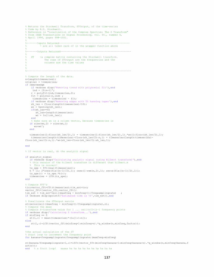
137
% Returns the Stockwell Transform, STOutput, of the time-series
% Code by R.G. Stockwell.
% Reference is "Localization of the Complex Spectrum: The S Transform"
% from IEEE Transactions on Signal Processing, vol. 44., number 4,
% April 1996, pages 998-1001.
%
%-------Inputs Returned------------------------------------------------
% - are all taken care of in the wrapper function above
%
%-------Outputs Returned------------------------------------------------
%
% ST -a complex matrix containing the Stockwell transform.
% The rows of STOutput are the frequencies and the
% columns are the time values
%
%
%-----------------------------------------------------------------------
% Compute the length of the data.
n=length(timeseries);
original = timeseries;
if removeedge
if verbose disp('Removing trend with polynomial fit'),end
ind = [0:n-1]';
r = polyfit(ind,timeseries,2);
fit = polyval(r,ind) ;
timeseries = timeseries - fit;
if verbose disp('Removing edges with 5% hanning taper'),end
sh_len = floor(length(timeseries)/10);
wn = hanning(sh_len);
if(sh_len==0)
sh_len=length(timeseries);
wn = 1&[1:sh_len];
end
% make sure wn is a column vector, because timeseries is
if size(wn,2) > size(wn,1)
wn=wn';
end
timeseries(1:floor(sh_len/2),1) = timeseries(1:floor(sh_len/2),1).*wn(1:floor(sh_len/2),1);
timeseries(length(timeseries)-floor(sh_len/2):n,1) = timeseries(length(timeseries)-
floor(sh_len/2):n,1).*wn(sh_len-floor(sh_len/2):sh_len,1);
end
% If vector is real, do the analytic signal
if analytic_signal
if verbose disp('Calculating analytic signal (using Hilbert transform)'),end
% this version of the hilbert transform is different than hilbert.m
% This is correct!
ts_spe = fft(real(timeseries));
h = [1; 2*ones(fix((n-1)/2),1); ones(1-rem(n,2),1); zeros(fix((n-1)/2),1)];
ts_spe(:) = ts_spe.*h(:);
timeseries = ifft(ts_spe);
end
% Compute FFT's
tic;vector_fft=fft(timeseries);tim_est=toc;
vector_fft=[vector_fft,vector_fft];
tim_est = tim_est*ceil((maxfreq - minfreq+1)/freqsamplingrate) ;
if verbose disp(sprintf('Estimated time is %f',tim_est)),end
% Preallocate the STOutput matrix
st=zeros(ceil((maxfreq - minfreq+1)/freqsamplingrate),n);
% Compute the mean
% Compute S-transform value for 1 ... ceil(n/2+1)-1 frequency points
if verbose disp('Calculating S transform...'),end
if minfreq == 0
st(1,:) = mean(timeseries)*(1&[1:1:n]);
else
st(1,:)=ifft(vector_fft(minfreq+1:minfreq+n).*g_window(n,minfreq,factor));
end
%the actual calculation of the ST
% Start loop to increment the frequency point
for banana=freqsamplingrate:freqsamplingrate:(maxfreq-minfreq)
st(banana/freqsamplingrate+1,:)=ifft(vector_fft(minfreq+banana+1:minfreq+banana+n).*g_window(n,minfreq+banana,f
actor));
end % a fruit loop! aaaaa ha ha ha ha ha ha ha ha ha ha

138
% End loop to increment the frequency point
if verbose disp('Finished Calculation'),end
%%% end strans function
%------------------------------------------------------------------------
function gauss=g_window(length,freq,factor)
% Function to compute the Gaussion window for
% function Stransform. g_window is used by function
% Stransform. Programmed by Eric Tittley
%
%-----Inputs Needed--------------------------
%
% length-the length of the Gaussian window
%
% freq-the frequency at which to evaluate
% the window.
% factor- the window-width factor
%
%-----Outputs Returned--------------------------
%
% gauss-The Gaussian window
%
vector(1,:)=[0:length-1];
vector(2,:)=[-length:-1];
vector=vector.^2;
vector=vector*(-factor*2*pi^2/freq^2);
% Compute the Gaussion window
gauss=sum(exp(vector));
%-----------------------------------------------------------------------
%^^^^^^^^^^^^^^^^^^^^^^^^^^^^^^^^^^^^^^^^^^^^^^^^^^^^^^^^^^^^^^^^^^^^^^^^^^%
function [ minfreq,maxfreq,samplingrate,freqsamplingrate] =
check_input(minfreq,maxfreq,samplingrate,freqsamplingrate,verbose,timeseries)
% this checks numbers, and replaces them with defaults if invalid
% if the parameters are passed as an array, put them into the appropriate variables
s = size(minfreq);
l = max(s);
if l > 1
if verbose disp('Array of inputs accepted.'),end
temp=minfreq;
minfreq = temp(1);;
if l > 1 maxfreq = temp(2);,end;
if l > 2 samplingrate = temp(3);,end;
if l > 3 freqsamplingrate = temp(4);,end;
if l > 4
if verbose disp('Ignoring extra input parameters.'),end
end;
end
if minfreq < 0 | minfreq > fix(length(timeseries)/2);
minfreq = 0;
if verbose disp('Minfreq < 0 or > Nyquist. Setting minfreq = 0.'),end
end
if maxfreq > length(timeseries)/2 | maxfreq < 0
maxfreq = fix(length(timeseries)/2);
if verbose disp(sprintf('Maxfreq < 0 or > Nyquist. Setting maxfreq = %d',maxfreq)),end
end
if minfreq > maxfreq
temporary = minfreq;
minfreq = maxfreq;
maxfreq = temporary;
clear temporary;
if verbose disp('Swapping maxfreq <=> minfreq.'),end
end
if samplingrate <0
samplingrate = abs(samplingrate);
if verbose disp('Samplingrate <0. Setting samplingrate to its absolute value.'),end
end
if freqsamplingrate < 0 % check 'what if freqsamplingrate > maxfreq - minfreq' case
freqsamplingrate = abs(freqsamplingrate);
if verbose disp('Frequency Samplingrate negative, taking absolute value'),end
end
% bloody odd how you don't end a function

139
%^^^^^^^^^^^^^^^^^^^^^^^^^^^^^^^^^^^^^^^^^^^^^^^^^^^^^^^^^^^^^^^^^^^^^^^^^^%
function st_help
disp(' ')
disp('st() HELP COMMAND')
disp('st() returns - 1 or an error message if it fails')
disp('USAGE:: [localspectra,timevector,freqvector] = st(timeseries)')
disp('NOTE:: The function st() sets default parameters then calls the function strans()')
disp(' ')
disp('You can call strans() directly and pass the following parameters')
disp(' **** Warning! These inputs are not checked if strans() is called directly!! ****')
disp('USAGE:: localspectra =
strans(timeseries,minfreq,maxfreq,samplingrate,freqsamplingrate,verbose,removeedge,analytic_signal,factor) ')
disp(' ')
disp('Default parameters (available in st.m)')
disp('VERBOSE - prints out informational messages throughout the function.')
disp('REMOVEEDGE - removes the edge with a 5% taper, and takes')
disp('FACTOR - the width factor of the localizing gaussian')
disp(' ie, a sinusoid of period 10 seconds has a ')
disp(' gaussian window of width factor*10 seconds.')
disp(' I usually use factor=1, but sometimes factor = 3')
disp(' to get better frequency resolution.')
disp(' ')
disp('Default input variables')
disp('MINFREQ - the lowest frequency in the ST result(Default=0)')
disp('MAXFREQ - the highest frequency in the ST result (Default=nyquist')
disp('SAMPLINGRATE - the time interval between successive data points (Default = 1)')
disp('FREQSAMPLINGRATE - the number of frequencies between samples in the ST results')
% end of st help procedure
function ha = tight_subplot(Nh, Nw, gap, marg_h, marg_w)
% tight_subplot creates "subplot" axes with adjustable gaps and margins
%
% ha = tight_subplot(Nh, Nw, gap, marg_h, marg_w)
%
% in: Nh number of axes in hight (vertical direction)
% Nw number of axes in width (horizontaldirection)
% gap gaps between the axes in normalized units (0...1)
% or [gap_h gap_w] for different gaps in height and width
% marg_h margins in height in normalized units (0...1)
% or [lower upper] for different lower and upper margins
% marg_w margins in width in normalized units (0...1)
% or [left right] for different left and right margins
%
% out: ha array of handles of the axes objects
% starting from upper left corner, going row-wise as in
% going row-wise as in
%
% Example: ha = tight_subplot(3,2,[.01 .03],[.1 .01],[.01 .01])
% for ii = 1:6; axes(ha(ii)); plot(randn(10,ii)); end
% set(ha(1:4),'XTickLabel',''); set(ha,'YTickLabel','')
% Pekka Kumpulainen 20.6.2010 @tut.fi
% Tampere University of Technology / Automation Science and Engineering
if nargin<3; gap = .02; end
if nargin<4 || isempty(marg_h); marg_h = .05; end
if nargin<5; marg_w = .05; end
if numel(gap)==1;
gap = [gap gap];
end
if numel(marg_w)==1;
marg_w = [marg_w marg_w];
end
if numel(marg_h)==1;
marg_h = [marg_h marg_h];
end
axh = (1-sum(marg_h)-(Nh-1)*gap(1))/Nh;
axw = (1-sum(marg_w)-(Nw-1)*gap(2))/Nw;
py = 1-marg_h(2)-axh;
ha = zeros(Nh*Nw,1);
ii = 0;

140
for ih = 1:Nh
px = marg_w(1);
for ix = 1:Nw
ii = ii+1;
ha(ii) = axes('Units','normalized', ...
'Position',[px py axw axh], ...
'XTickLabel','', ...
'YTickLabel','');
px = px+axw+gap(2);
end
py = py-axh-gap(1);
end

141
9.4. Appendix D: HFOs Detected During Seizure
Patient WDH-022 has endured a seizure at 14:14:34, 10/22/2014. The electrode placement for this
patient is provided in the table below. One HFO Figure has been plotted for each iEEG channel in
n the figures below.
Name of the electrode grid Placement
A 32-contact grid array (D) The electrode strip was placed over the left frontal convexity. Contact 1 was most posterior and superior, 8 most posterior and inferior, 25 most anterior and superior and 32 most anterior and inferior.
A 32-contact grid array (C) It was placed over the left frontoparietal convexity. Contact 1 was most posterior and superior, 8 most posterior and inferior, 25 most anterior and superior and 32 most anterior and inferior.
A 4-contact strip (A) The electrode array was placed on the left parietal convexity, posterior to grid D. Contact 1 was posterior and 4 was anterior.
A 4 –contact Strip (B) It was placed on the left parietal convexity, inferior to strip A. Contact 1 was posterior and 4 was anterior.
An 8-contact strip (E) It was placed over the left inferior frontal/orbitofrontal region, with contact 1 being anterior and 8 posterior.
An 8-contact strip (F) This electrode array was placed over the superior lateral left temporal region, with contact 1 being anterior and 8 posterior.

142
iEEG channel A1 - left parietal convexity iEEG channel A2 - left parietal convexity

143
iEEG channel A3 - left parietal convexity iEEG channel A4 - left parietal convexity

144
iEEG channel B1 - left parietal convexity iEEG channel B2 - left parietal convexity

145
iEEG channel B3 - left parietal convexity iEEG channel B4 - left parietal convexity
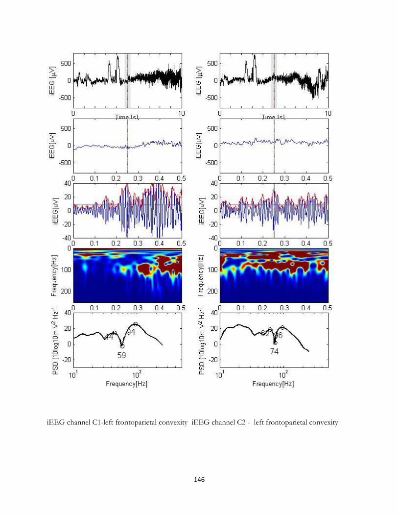
146
iEEG channel C1-left frontoparietal convexity iEEG channel C2 - left frontoparietal convexity

147
iEEG channel C5-left frontoparietal convexity iEEG channel C6 - left frontoparietal convexity

148
iEEG channel C7-left frontoparietal convexity iEEG channel C8 - left frontoparietal convexity

149
iEEG channel C9-left frontoparietal convexity iEEG channel C10 - left frontoparietal convexity

150
iEEG channel C11-left frontoparietal convexity iEEG channel C12 - left frontoparietal convexity

151
iEEG channel C13-left frontoparietal convexity iEEG channel C14 - left frontoparietal convexity

152
iEEG channel C15-left frontoparietal convexity iEEG channel C3 - left frontoparietal convexity

153
iEEG channel C4-left frontoparietal convexity iEEG channel C16 - left frontoparietal convexity

154
iEEG channel C17- left frontoparietal convexity iEEG channel C18 - left frontoparietal convexity

155
iEEG channel C19-left frontoparietal convexity iEEG channel C20 - left frontoparietal convexity

156
iEEG channel C21- left frontoparietal convexity iEEG channel C22- left frontoparietal convexity

157
iEEG channel C23- left frontoparietal convexity iEEG channel C24 - left frontoparietal convexity

158
iEEG channel C25- left frontoparietal convexity iEEG channel C26 - left frontoparietal convexity

159
iEEG channel C27 left frontoparietal convexity iEEG channel C28 - left frontoparietal convexity

160
iEEG channel C29- left frontoparietal convexity iEEG channel C30 - left frontoparietal convexity
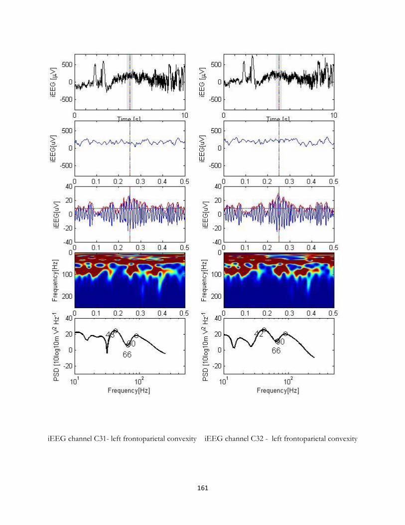
161
iEEG channel C31- left frontoparietal convexity iEEG channel C32 - left frontoparietal convexity

162
iEEG channel D1- left frontal convexity iEEG channel D2 - left frontal convexity

163
iEEG channel D3- left frontal convexity iEEG channel D4 - left frontal convexity

164
iEEG channel D5- left frontal convexity iEEG channel D6- left frontal convexity

165
iEEG channel D7- left frontal convexity iEEG channel D8 - left frontal convexity

166
iEEG channel D9- left frontal convexity iEEG channel D10 - left frontal convexity

167
iEEG channel D11- left frontal convexity iEEG channel D12- left frontal convexity

168
iEEG channel D13- left frontal convexity iEEG channel D14- left frontal convexity

169
iEEG channel D15- left frontal convexity iEEG channel D16- left frontal convexity

170
iEEG channel D17- left frontal convexity iEEG channel D18- left frontal convexity

171
iEEG channel D19- left frontal convexity iEEG channel D20- left frontal convexity

172
iEEG channel D21- left frontal convexity iEEG channel D22- left frontal convexity

173
iEEG channel D23- left frontal convexity iEEG channel D24- left frontal convexity

174
iEEG channel D25- left frontal convexity iEEG channel D26- left frontal convexity

175
iEEG channel D27- left frontal convexity iEEG channel D28- left frontal convexity

176
iEEG channel D29- left frontal convexity iEEG channel D30- left frontal convexity

177
iEEG channel D31- left frontal convexity iEEG channel D32- left frontal convexity

178
iEEG channel E1- left inferior frontal region iEEG channel E2- left inferior frontal region

179
iEEG channel E3- left inferior frontal region iEEG channel E4- left inferior frontal region

180
iEEG channel E5- left inferior frontal region iEEG channel E6- left inferior frontal region

181
iEEG channel F1- superior lateral left temporal region iEEG channel F2- superior lateral left temporal region

182
iEEG channel F3- superior lateral left temporal region iEEG channel F4- superior lateral left temporal region

183
iEEG channel F5- superior lateral left temporal region iEEG channel F6- superior lateral left temporal region

184
iEEG channel F7- superior lateral left temporal region iEEG channel F8- superior lateral left temporal region