Human Capital and Development Accounting: New Evidence ...

Human Capital and Development Accounting: New

Evidence from Wage Gains at Migration⇤

Lutz Hendricks† Todd Schoellman‡

June 2016

Abstract

We reconsider the role for human capital in accounting for cross-country income

di↵erences. Our contribution is to bring to bear new data on the pre- and post-

migration labor market experiences of immigrants to the U.S. Immigrants from poor

countries experience wage gains that are only 40 percent of the GDP per worker gap,

which implies that “country” accounts for 40 percent of income di↵erences, while

human capital accounts for 60 percent. Our approach handles selection by comparing

the wage of the same individual in two di↵erent countries. We also provide evidence

on and a correction for skill transfer.

JEL Classification: O11, J31

⇤We thank Mark Bils for a thoughtful discussion and seminar and conference participants at ArizonaState University, the Federal Reserve Bank of Philadelphia, the Federal Reserve Bank of Chicago, theUniversity of Pittsburgh, the 2014 SED, the 2015 Conference on Growth and Development, and the 2016NBER EFJK meeting for helpful comments.

†University of North Carolina, Chapel Hill. E-mail: [email protected]‡Arizona State University. E-mail: [email protected]

1

1 Introduction

One of the central challenges for economists is to explain the large di↵erences in gross

domestic product (GDP) per worker across countries. Development accounting provides a

useful first step toward this goal. It measures the relative contribution of physical capital,

human capital, and total factor productivity (TFP) in accounting for cross-country income

di↵erences. These accounting results can help highlight the types of theories or mechanisms

most likely to explain cross-country income di↵erences. For example, the consensus in

the literature is that physical capital accounts for a small fraction of income di↵erences,

which has suggested to researchers to de-emphasize theories that assign a prominent role

to variation in physical capital per worker.1

The main unsettled question in this literature is the relative importance of TFP versus

human capital in accounting for cross-country income di↵erences. The literature has tried

a number of approaches to measuring human capital and reached little consensus on the

answer. Since TFP is measured as a residual explanatory factor, wide variation in measured

human capital stocks implies wide variation in measured TFP and hence substantial dis-

agreement about the relative contribution of the two. For example, the literature has found

that human accounts for anywhere from one-fifth to four-fifths of cross-country income

di↵erences, with TFP in turn accounting for anywhere from three-fifths to none.2

Our contribution to this debate is to provide new evidence drawing on the experiences of

immigrants to the United States (U.S.). Intuitively, immigrants provide valuable infor-

mation because they enter the U.S. with the human capital they acquired in their birth

country, but not the physical capital or TFP. Hence, their labor market performance in the

U.S. conveys information about their human capital separated from the other two country-

specific factors. On the other hand, working with immigrants presents two well-known

challenges. First, immigrants are selected: their human capital is not the same as the hu-

man capital of a randomly chosen person in their birth country. Second, their labor market

performance may not accurately reflect their human capital if skills transfer imperfectly

across countries.3

1See for example Klenow and Rodriguez-Clare (1997), Hall and Jones (1999), Caselli (2005), or Hsiehand Klenow (2010) for classic references on development accounting and its interpretation.

2The former figure comes from Hall and Jones (1999); the latter comes from Manuelli and Seshadri(2014) or Jones (2014). The literature also includes a wide range of estimates in between. See, for example,Erosa et al. (2010), Hanushek and Woessmann (2012), Cordoba and Ripoll (2013), Weil (2007), or Cubaset al. (forthcoming).

3Previous papers that have investigated immigrants and cross-country di↵erences in human capitalinclude Hendricks (2002), Schoellman (2012), Schoellman (forthcoming), and Lagakos et al. (2015).

2

We address these challenges by utilizing new data from the New Immigrant Survey (NIS),

a sample of adult immigrants granted lawful permanent residence in the U.S. in 2003 (col-

loquially, green card recipients) (Jasso et al., n.d.). The unique advantage of this dataset is

that it asked immigrants detailed questions about both their pre- and post-migration labor

market experiences.4 We use this data in three ways. First, we construct a measure of

the importance of human capital for development accounting based on immigrants’ wage

gains at migration. Second, we address the challenge of selection by comparing the pre-

migration characteristics of immigrants to non-migrants. Third, we address the challenge

of skill transferability by comparing the pre- to post-migration occupations of immigrants.

We start by revisiting the standard development accounting framework. We describe the

assumptions that are necessary to draw aggregate implications from the labor market expe-

riences of immigrants. We show that the most direct measure of the importance of physical

capital and TFP is the log-wage gain at migration relative to the log di↵erence in GDP per

worker. Intuitively, the idea is that an immigrant has the same human capital but di↵erent

physical capital and TFP before and after migrating. The wage gain at migration is thus

an index of the relative importance of these country-specific factors, while the residual can

be attributed to gaps in human capital per worker.5 In addition to simplicity, this measure

also has the useful feature that it controls for selection in a straightforward manner by

studying the wages of the exact same worker in two di↵erent countries.

Our empirical work thus relies heavily on a comparison of pre- to post-migration wages. The

NIS o↵ers carefully constructed and detailed wage data. It surveyed immigrants about up

to two pre-migration jobs and up to two post-migration jobs. It also allowed for a great deal

of flexibility in how workers report their earnings. They could report their pre-migration

earnings from working in any country, denominated in any currency, from any reference

year, at whatever pay frequency they preferred. We discuss in detail how we adjust these

data for exchange rate, purchasing power parity, and di↵erences in reporting year to arrive

at estimates of their pre-migration and post-migration hourly wages both denominated in

real PPP-adjusted U.S. dollars. We also provide detailed information on sensitivity and

robustness checks to possible confounding issues such as episodes of inflation or currency

revaluation, migrants who report working in their non-birth country, and so on.

4We are not the first to use the pre-migration labor market information in the NIS. Probably the mostrelated work is Rosenzweig (2010). The goal of this paper is to use immigrants’ experiences to estimate arich and flexible set of prices for a variety of skills. While useful, this evidence is di�cult to interpret froma development accounting perspective.

5A related literature have used models of the wage gain at migration to quantify the welfare gains fromfreer migration across countries (Klein and Ventura, 2009; Kennan, 2013).

3

We use these data to construct the log wage change at migration relative to the log gap in

GDP per worker. We focus on immigrants from poor countries, with PPP GDP per worker

less than one-fourth the U.S. level. We find that the average wage gain at migration is

40 percent of the total gap in GDP per worker, implying that 40 percent of cross-country

income di↵erences are accounted for by physical capital and TFP, with the remaining 60

percent accounted for by human capital. We show that this figure is robust to many of

the details of sample selection and wage construction. For example, similar results hold for

immigrants who entered the U.S. with very di↵erent education levels and on very di↵erent

visas.

This finding attributes a much higher share to human capital than earlier papers in the

literature that used immigrant earnings (Hendricks, 2002; Schoellman, 2012). These earlier

papers lacked data on pre-migration wages and so drew inferences based on a comparison

of the post-migration wages of immigrants from poor and rich countries. The underlying

assumption was that immigrants from poor countries and rich countries are similarly se-

lected. Our data allow us to control for selection directly. We can also go a step further

and back out the implied degree of selection by comparing the pre-migration characteris-

tics of immigrants to those of non-migrants. We find that immigrants are highly selected

on characteristics such as education or wages, and that immigrants from poor countries

are much more selected on these characteristics than immigrants from rich countries. The

correlation between selection and birth country development biased the inferences in the

existing literature.

The data also allow us to speak directly to two other important issues. The first is the trans-

ferability of immigrants’ skills. To investigate this issue, we compare the pre-migration and

post-migration occupations of immigrants. We find most immigrants switch occupations

upon migration. Further, we find that most immigrants experience occupational downgrad-

ing, meaning that their post-migration occupation is lower-paying than their pre-migration

occupation, as judged by the mean wage of natives in those occupations. To the extent

that this occupational downgrading represents imperfect skill transfer, it implies that we

may be understating post-migration wages and the wage gains at migration, which would

lead us to understate the role of country and overstate the role of human capital. We inves-

tigate several ways to adjust for occupational downgrading and find that doing so lowers

the human capital share to roughly one-half.

The second issue we can speak to is how to aggregate labor provided by workers with dif-

ferent education levels. Although the development accounting literature usually assumes

4

that they are perfect substitutes, Jones (2014) has recently shown that allowing for imper-

fect substitution would dramatically raise the importance of human capital in development

accounting. The experiences of immigrants are useful for thinking about this issue because

immigrants from poor countries move from a country where educated labor is scarce to one

where it is abundant. If workers with di↵erent education levels are imperfect substitutes,

then this implies that more educated immigrants should gain less at migration relative to

less educated immigrants. Empirically, we find that wage gains are very similar across edu-

cation groups. We conclude that a model with perfect substitution across education types

fits our data well, although we have relatively few very uneducated immigrants.

The rest of the paper proceeds as follows. Section 2 introduces the development accounting

framework and the mapping from our micro-evidence on immigrants to aggregate cross-

country income di↵erences. Section 3 discusses the data and how we construct comparable

pre- and post-migration hourly wages. Section 4 provides the main results and their ro-

bustness. Section 5 quantifies the importance of selection and Section 6 the importance

of skill transferability. Section 7 investigates the elasticity of substitution between workers

with di↵erent skill levels. Section 8 concludes.

2 Development Accounting Framework

We begin by outlining our accounting framework, which follows the literature closely (see

Caselli (2005) or Hsieh and Klenow (2010) for recent overviews). Our particular focus here

is on clarifying the assumptions needed to draw aggregate inferences from evidence on the

wage gains at immigration. We start with the standard aggregate production function,

Yc = K↵c (AcHc)

1�↵

where Yc is country c’s PPP-adjusted GDP, Kc is its physical capital stock, Ac is its to-

tal factory productivity, and Hc ⌘ hcLc is the total labor input, which in turn can be

decomposed into human capital per worker hc and the number of workers Lc.

Following Klenow and Rodriguez-Clare (1997), we re-write the production function in per

worker terms:

yc =

✓Kc

Yc

◆↵/(1�↵)

Achc (1)

5

where yc denotes PPP-adjusted GDP per worker. It is well-known that there is large vari-

ation in this object across countries. The goal of development accounting is to decompose

variation in y into variation in three components, given on the right-hand side: capital-

output ratios; total factor productivity; and average human capital. In this paper we focus

primarily on distinguishing the share of human capital versus the other two factors jointly,

so we define zc ⌘ (Kc/Yc)↵/(1�↵) Ac. We call this term the e↵ect of country, because it is

what changes when immigrants move to a new country, while their human capital remains

the same.

We conduct our accounting exercises in log-levels. Doing so produces results that are

additive and order-invariant. Our focus is on separating the relative contribution of human

capital from the other two terms in accounting for the di↵erence in PPP GDP per worker

between c and c0:

1 =log(zc)� log(zc0)

log(yc)� log(yc0)+

log(hc)� log(hc0)

log(yc)� log(yc0)

⌘ sharecountry

+ sharehuman capital

(2)

Our goal is to provide guidance on the decomposition between human capital and country

for development accounting.

2.1 Wage Gains of Immigrants and Development Accounting Im-

plications

We use the wages of immigrants to inform us about the role of country and human capital

for development accounting. Our approach builds on the insights of Bils and Klenow (2000),

who showed that wages are informative about human capital under two assumptions. First,

workers of di↵erent types are assumed to be perfect substitutes. In this case, workers

may provide varying quantities of human capital, but the total labor supply is simply the

total human capital of all workers. Second, labor markets are assumed to be perfectly

competitive, so that workers are paid their marginal product. Given these assumptions,

the representative firm hires a total quantity Hc of human capital at the prevailing wage

per unit of human capital !c to maximize profits:

maxHc

K↵c (AcHc)

1�↵ � !cHc.

6

The first-order condition of the firm implies that the wage per unit of human capital is

!c = (1� ↵)zc, where zc is defined as in the previous subsection.

The observed hourly wage of of worker i in country c wi,c is then the product of the wage

per unit of human capital and the amount of human capital they possess:

log(wi,c) = log [(1� ↵)zc] + log(hi). (3)

Given that we have data on both pre- and post-migration wages of immigrants, we can

construct the log-wage gain to migration. If we divide this by the log-GDP per worker

di↵erence between c and U.S., we find a direct measure of the importance of countries:

log(wi,U.S.)� log(wi,c)

log(yU.S.)� log(yc)=

log(zU.S.)� log(zc)

log(yU.S.)� log(yc)= share

country

(4)

We construct sharehuman capital

⌘ 1� sharecountry

. Intuitively, the idea is that a worker who

migrates keeps their same human capital but switches physical capital and TFP levels. We

study how much this changes their wages relative to the total gap in GDP per worker.

If the change in wages is as large as the gap in GDP per worker, then we conclude that

country explained all of cross-country income di↵erences, with no role for human capital.

If there is no change in wages, then we conclude that human capital explained all of cross-

country income di↵erences, with no role for country. Our goal is to calculate where we

stand between these two polar cases.

A few remarks are in order at this point. First, note that this statistic controls for the usual

selection concern, namely that immigrants may be more talented or harder-working than

non-migrants, because it uses wage observations from the same worker in two countries. In

Section 5 we actually quantify the extent of selection by comparing the pre-migration wages

of immigrants to the wages of non-migrants. A more subtle concern is that immigrants may

be selected on their gains to migration. We provide a simple model of this in Appendix

D.1. The main intuition is that if immigrants are positively selected on gains to migration

(as in McKenzie et al. (2010)), then we provide an upper bound on the gains to migration

and a lower bound on the share of human capital in development accounting.6 Second,

this simple equation assumes that skills transfer perfectly upon migration; we revisit this

point in Section 6. Finally, we have maintained so far the assumption of perfect substitutes

6Similar logic shows that a binding minimum wage would also imply that we are calculating a lowerbound on the share of human capital in development accounting. However, less than five percent of oursample is paid at or below the minimum wage.

7

across skill groups that is common in most of the literature, but we revisit this point in

Section 7. We now turn to the data.

3 New Immigrant Survey

The New Immigrant Survey (NIS) is a nationally representative sample of adult immigrants

granted lawful permanent residence (colloquially, green card recipients) between May and

November of 2003, drawn from government administrative records (Jasso et al., 2005, n.d.).

Our sample is roughly equally split between newly-arrived immigrants granted lawful per-

manent residency from abroad and immigrants who adjusted to lawful permanent residency

after previously entering the U.S. through other means. The focus on legal permanent resi-

dents leads to some di↵erences between NIS respondents and those in other samples. Most

notably, there are few Mexicans in this sample, as compared to the Census. More gener-

ally, immigrants in the NIS are a little younger, better educated, and lower paid than in

the Census or the American Community Survey. Nonetheless, the key stylized facts of the

literature obtain in the NIS sample as well. See Appendix C for details.

The NIS includes four main sets of information that we exploit. First, it surveys respondents

about the usual set of demographic characteristics, such as age and education. Second, it

contains administrative data on the type of visa they used to enter the U.S. Third, it

surveys them about their labor market experiences in the U.S. It contains information on

their current job at the time of the survey and their first post-migration job (if di↵erent).

Fourth, it surveys them about their pre-migration experiences, particularly their labor

market experiences. Immigrants were surveyed about up to two jobs before entry, their

first (after age 16) and last (if di↵erent than the first). Throughout, we focus on the most

recent pre-migration job. For all jobs we know standard information such as occupation,

industry, earnings, and hours and weeks worked.

Given our focus on pre-migration wages of immigrants and the wage gains at migration, it is

important that immigrants’ reported wages be accurate. Fortunately, the NIS was careful

to allow immigrants a great deal of flexibility in reporting their pre-migration earnings.

Immigrants reported both how much they earned and the frequency at which they were

paid (hourly, daily, weekly, monthly, annual, etc.). They also chose what year this report

pertains to; what country they were working in; and what currency they were paid in.

This flexibility is important because it allows immigrants to report earnings in the most

natural way for them, rather than forcing them to do conversions. It also allows for unusual

8

or non-obvious situations, such as the widespread use of the U.S. dollar as a medium of

payment even outside of the U.S., or the tendency for European migrants to remember

their earnings denominated in both pre-euro currencies or euros.

Of course, this flexibility necessitates a great deal of adjustment on our part. First, we use

the reported earnings and payment frequency to construct hourly wage for all immigrants.

Second, we translate the currency to U.S. dollars by using the market exchange rate between

the reported currency and the U.S. dollar prevailing at the time, taken from the Penn World

Tables.7 Third, we adjust wages for the purchasing power parity prevailing in the country at

the time, again taken from the Penn World Tables.8 Note that in cases where workers report

the “natural” currency for their country (e.g., pesos in Mexico) these first two adjustments

are equivalent to simply dividing by the PPP exchange rate.

There are two potential complications to these adjustments that we discuss here and explore

further in our robustness section. First, some immigrants report being paid in currencies

that have experienced large changes in value or revaluations. Second, some immigrants

report unusual currency-country pairs, for example being paid in lira in Brazil. In each

case, we are concerned about measurement error: that immigrants may be misremembering

the currency or the year in which they were paid, and that doing so could substantially

alter the implied wage. Following the advice of the NIS manuals, we exclude all immigrants

who were paid in currencies with subsequent revaluations. We also flag all immigrants who

report being paid in currencies that ever had a devaluation or experienced high inflation but

not a devaluation; or immigrants who report unusual currency-country pairs.9 We explore

robustness to excluding these groups.

At this point we have an estimate of pre-migration wages from year t converted into U.S.

dollars and adjusted for cost of living, as well as up to two observations on post-migration

wages. Conceptually, our goal is simple: we want to compute the wage gain at migration.

This calculation is complicated by immigrant assimilation: immigrants’ occupational sta-

tus, wages, and earnings are generally found to grow more quickly than those of comparable

natives in the years after migration (Akresh, 2008; Duleep, 2015). There are three interpre-

7We use PWT 7.1 for most countries. Our pre-euro European exchange rates come from PWT 6.2;our pre-dollarization Ecuadorian exchange rate from PWT 6.1; and our exchange rate for the U.S.SR,Czechoslovakia, Yugoslavia, and Myanmar come from PWT 5.6 (Heston et al., 2012, 2006, 2002, n.d.).

8This object was provided directly and called price level (P ) in some editions of the Penn World Table; inothers it is constructed as the ratio of purchasing power parity to nominal exchange rates (PPP/XRAT ).

9Inflation data comes from the World Bank (2014). Data on currency-country pairs come mostly fromthe Penn World Tables and the CIA Factbook; we have also allowed some pairs where a currency is notthe o�cial currency of a country but has been in common use, such as the U.S. dollar in former Sovieteconomies in the 1990s.

9

tations of this fact. First, it could be that initial wages are temporarily depressed by the

absence of “search capital”, meaning that immigrants have not yet found a job that suits

and values their talents; in this case it would be preferable to focus on a later job. Second, it

could be that immigrants acquire human capital more rapidly than natives after migration,

perhaps in response to the change in environment; in this case it would be preferable to

focus on an earlier job. Finally, it could be that immigrant wage patterns are driven by a

composition e↵ect through selective return migration based on wages; in this case it would

be preferable to focus on an earlier job (Lubotsky, 2007). There is no clear consensus in

the literature about the relative importance of these three e↵ects.

In the face of this ambiguity we consider a wide range of possibilities. Our baseline results

use immigrants’ later job, from 2003–04. We convert this into a year t wage by netting

o↵ the wage growth of observably similar natives between year t and 2003, where we use

age, gender, and education as our observable characteristics.10 This adjustment corrects

for inflation and life-cycle wage growth. Any wage growth in excess of that of observably

similar natives (assimilation) is included in our post-migration wages and the wage gains

at migration. We do this because it will tend to increase reported post-migration wages

and wage gains at migration, which makes our calculations more conservative. We include

in the baseline sample anyone whose last pre-migration wage is from the years 1983–2003.

Below, we consider robustness to using instead the first rather than current job in the U.S.,

and to focusing on subsets of immigrants whose last pre-migration wage was from earlier

or later years.

After these checks, the remaining immigrants from poor countries have straightforward

immigration-job histories. For example, more than three-fourths of the resulting sample

had never lived outside their birth country for more than six months before permanently

immigrating to the U.S. Again, more than three-fourths report working their first U.S. job

within one year of their last pre-migration job; more than 70 percent of immigrants satisfy

both restrictions. We show below that our results are robust to focusing on this group. We

trim a small number of outliers that report being paid less than $0.01 or more than $1,000

per hour; we find similar results if we implement stricter rules for trimming outliers. The

final sample includes 1,383 immigrants with data on both pre- and post-migration wages

that we use for our exercises. Table A1 in Appendix A shows the number of immigrants

dropped by each of our sample restrictions.

Recall that our goal is to compare the log-wage change at migration to the log di↵erence

10Data from the Current Population Survey. See Appendix B for details.

10

Table 1: Most Sampled Countries by GDP per Worker Category

PPP GDP p.w. Category Most Sampled Countries

< 1/16 Ethiopia, Nepal, Nigeria

1/16� 1/8 India, Philippines, China

1/8� 1/4 Dominican Republic, Ukraine, Albania

1/4� 1/2 Poland, Mexico, Russia

> 1/2 Canada, United Kingdom, KoreaTable note: Lists the three most common birth countries in each PPP GDP per workercategory in the sample.

in GDP per worker. Our measure of the latter is the log-di↵erence in GDP per worker

between the U.S. and country b in 2005 from PWT 7.1, although all of our results hold

if we use year-of-migration gaps in GDP per worker instead. Confidentiality restrictions

prevent us from reporting statistics by country of origin in all but a few cases. For this

reason our baseline approach is to report statistics for each of five PPP GDP per worker

categories: less than 1/16th U.S. income; 1/16–1/8; 1/8–1/4; 1/4–1/2; and more than half.

Table 1 lists the three countries with the most observations within each category.

4 Results

We now turn to our results. We begin by discussing the basic patterns of wages, which we

report in year 2003 U.S. dollars. We compute the mean pre- and post-migration log wage

by PPP GDP per worker category. We plot the exponentiated results in Figure 1a, with the

exact figures given in Table 2. Both pre- and post-migration wages are positively correlated

with development, although the trend is surprisingly weak among the three middle income

categories. More striking are the high levels of pre-migration wages for immigrants from

poor countries: the reported figures correspond to a PPP-adjusted hourly wage of $2.88

per hour even for immigrants from the very poorest countries.

A key statistic for our approach is the wage gain at migration, which we compute for each

individual as the log of the ratio of post-migration to pre-migration wages. We average this

figure by PPP GDP per worker category and plot the exponentiated results in Figure 1b,

with the exact figures given in Table 2. The average immigrant has a substantial wage gain

at migration. The extent of the gain is negatively correlated with development, as one would

expect; immigrants from the poorest countries gain by a factor of 2.9, while immigrants

11

Figure 1: Wages, Wage Gains, and GDP per worker

(a) Pre- and Post-Migration Wages

2003 Mean U.S. Wage

0

5

10

15

20

25

Hou

rly W

age,

200

3 U

S D

olla

rs

<1/16 1/16–1/8 1/8–1/4 1/4–1/2 >1/2PPP GDP per worker relative to U.S., 2005

Pre-Migration Wage Post-Migration Wage

(b) Wage Gains at Migration

0

1

2

3

4

Rat

io o

f Pos

t to

Pre–

Mig

ratio

n W

age


from the richest gain factor of 1.3. The gains for immigrants from poor countries are quite

small relative to the gap in GDP per worker, suggesting that “country” plays a small role

in development accounting. We formalize this idea in the next subsection.

4.1 Accounting Implications

Recall from equation (4) that our measure of the importance of human capital is one minus

the log-wage change at migration relative to the log-GDP per worker gap. We implement

this idea by constructing the implied share for every immigrant in our sample. We then

compute the mean of the share within each PPP GDP per worker category. The resulting

estimates and 95 percent confidence intervals for each GDP per worker category are given

in Table 2.11

Our primary focus is on poor countries because they are of greater interest for develop-

ment accounting. The estimates from the three poorest income groups agree closely on an

estimate in the range of 0.55–0.69 with fairly tight confidence intervals. For most of our

results we pool these three income groups; when combined, the implied share of human

capital in development accounting is 60 percent against a share of country-specific factors

11We find very similar results if we use instead the median of the implied human capital shares, or if wefirst compute mean log-wage changes at migration and mean log-GDP per worker gaps and then constructthe implied human capital share. Our confidence intervals are constructed using a normal approximation,but bootstrapped confidence intervals are very similar.

12

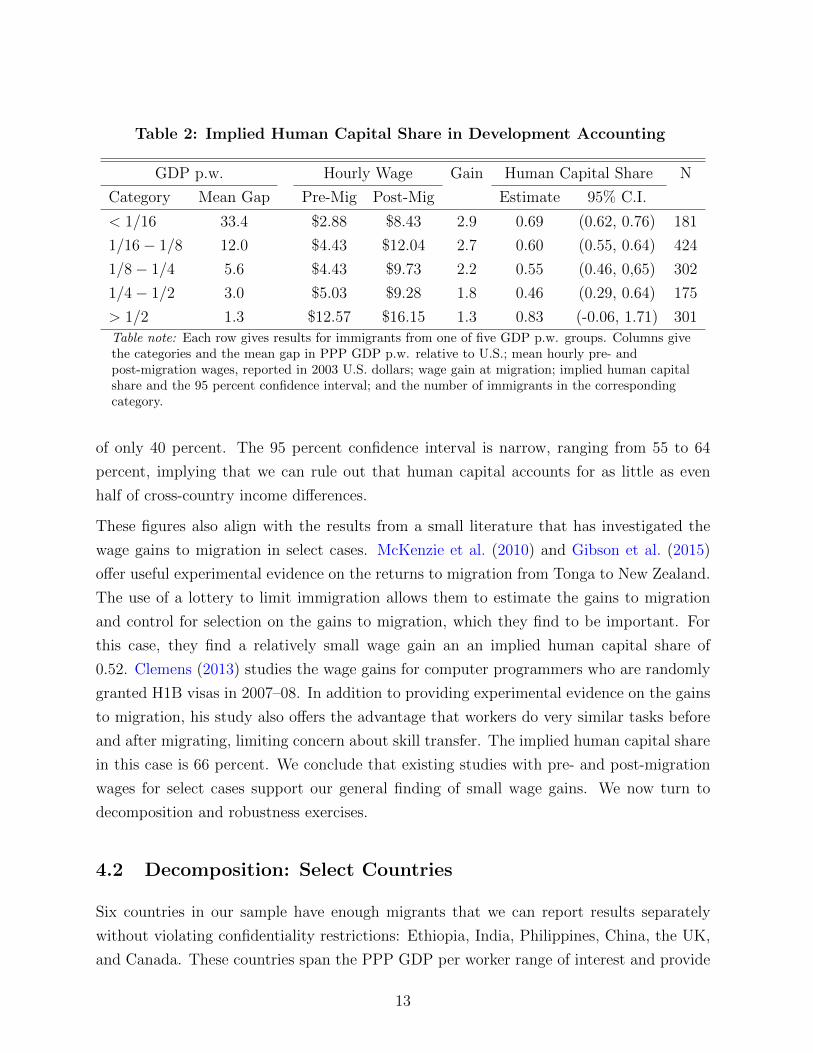
Table 2: Implied Human Capital Share in Development Accounting

GDP p.w. Hourly Wage Gain Human Capital Share N

Category Mean Gap Pre-Mig Post-Mig Estimate 95% C.I.

< 1/16 33.4 $2.88 $8.43 2.9 0.69 (0.62, 0.76) 181

1/16� 1/8 12.0 $4.43 $12.04 2.7 0.60 (0.55, 0.64) 424

1/8� 1/4 5.6 $4.43 $9.73 2.2 0.55 (0.46, 0,65) 302

1/4� 1/2 3.0 $5.03 $9.28 1.8 0.46 (0.29, 0.64) 175

> 1/2 1.3 $12.57 $16.15 1.3 0.83 (-0.06, 1.71) 301Table note: Each row gives results for immigrants from one of five GDP p.w. groups. Columns givethe categories and the mean gap in PPP GDP p.w. relative to U.S.; mean hourly pre- andpost-migration wages, reported in 2003 U.S. dollars; wage gain at migration; implied human capitalshare and the 95 percent confidence interval; and the number of immigrants in the correspondingcategory.

of only 40 percent. The 95 percent confidence interval is narrow, ranging from 55 to 64

percent, implying that we can rule out that human capital accounts for as little as even

half of cross-country income di↵erences.

These figures also align with the results from a small literature that has investigated the

wage gains to migration in select cases. McKenzie et al. (2010) and Gibson et al. (2015)

o↵er useful experimental evidence on the returns to migration from Tonga to New Zealand.

The use of a lottery to limit immigration allows them to estimate the gains to migration

and control for selection on the gains to migration, which they find to be important. For

this case, they find a relatively small wage gain an an implied human capital share of

0.52. Clemens (2013) studies the wage gains for computer programmers who are randomly

granted H1B visas in 2007–08. In addition to providing experimental evidence on the gains

to migration, his study also o↵ers the advantage that workers do very similar tasks before

and after migrating, limiting concern about skill transfer. The implied human capital share

in this case is 66 percent. We conclude that existing studies with pre- and post-migration

wages for select cases support our general finding of small wage gains. We now turn to

decomposition and robustness exercises.

4.2 Decomposition: Select Countries

Six countries in our sample have enough migrants that we can report results separately

without violating confidentiality restrictions: Ethiopia, India, Philippines, China, the UK,

and Canada. These countries span the PPP GDP per worker range of interest and provide

13

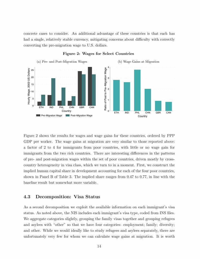
concrete cases to consider. An additional advantage of these countries is that each has

had a single, relatively stable currency, mitigating concerns about di�culty with correctly

converting the pre-migration wage to U.S. dollars.

Figure 2: Wages for Select Countries


0

5

10

15

20

25

Hou

rly W

age,

200

3 U

S D

olla

rs

ETH IND PHL CHN GBR CANCountry

Pre–Migration Wage Post–Migration Wage


0

1

2

3

4

Rat

io o

f Pos

t to

Pre–

Mig

ratio

n W

age

ETH IND PHL CHN GBR CANCountry

Figure 2 shows the results for wages and wage gains for these countries, ordered by PPP

GDP per worker. The wage gains at migration are very similar to those reported above:

a factor of 2 to 4 for immigrants from poor countries, with little or no wage gain for

immigrants from the two rich countries. There are interesting di↵erences in the patterns

of pre- and post-migration wages within the set of poor countries, driven mostly by cross-

country heterogeneity in visa class, which we turn to in a moment. First, we construct the

implied human capital share in development accounting for each of the four poor countries,

shown in Panel B of Table 3. The implied share ranges from 0.47 to 0.77, in line with the

baseline result but somewhat more variable.

4.3 Decomposition: Visa Status

As a second decomposition we exploit the available information on each immigrant’s visa

status. As noted above, the NIS includes each immigrant’s visa type, coded from INS files.

We aggregate categories slightly, grouping the family visas together and grouping refugees

and asylees with “other” so that we have four categories: employment; family; diversity;

and other. While we would ideally like to study refugees and asylees separately, there are

unfortunately very few for whom we can calculate wage gains at migration. It is worth

14

Table 3: Human Capital Share in Development Accounting by Subgroups

Robustness Check Human Capital Share 95% Confidence Interval N

Panel A: Baseline

Baseline 0.60 (0.55, 0.64) 907

Panel B: Decomposition by Country

Ethiopia 0.77 (0.67, 0.86) 41

India 0.63 (0.58, 0.69) 167

Philippines 0.47 (0.39, 0.55) 111

China 0.70 (0.57, 0.83) 63

Panel C: Decomposition by Visa Status

Employment visa 0.52 (0.46, 0.59) 196

Family visa 0.64 (0.53, 0.74) 148

Diversity visa 0.58 (0.49, 0.67) 186

Other visa 0.58 (0.47, 0.68) 121Table note: Each column shows the implied human capital share in development accounting (oneminus the wage gain at migration relative to the GDP per worker gap); the 95 percent confidenceinterval for that statistic; and the number of immigrants in the corresponding sample. Each rowgives the result from constructing these statistics for a di↵erent sample or using di↵erent measuresof pre-migration wages, post-migration wages, or the GDP per worker gap.

15

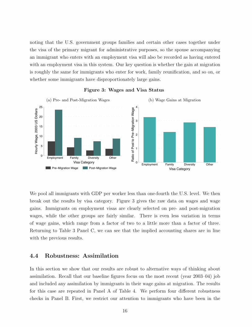
noting that the U.S. government groups families and certain other cases together under

the visa of the primary migrant for administrative purposes, so the spouse accompanying

an immigrant who enters with an employment visa will also be recorded as having entered

with an employment visa in this system. Our key question is whether the gain at migration

is roughly the same for immigrants who enter for work, family reunification, and so on, or

whether some immigrants have disproportionately large gains.

Figure 3: Wages and Visa Status


0

5

10

15

20

25

Hour

ly W

age,

200

3 US

Dol

lars

Employment Family Diversity OtherVisa Category



0

1

2

3

4

Ratio

of P

ost t

o Pr

e–M

igra

tion

Wag

e

Employment Family Diversity OtherVisa Category

We pool all immigrants with GDP per worker less than one-fourth the U.S. level. We then

break out the results by visa category. Figure 3 gives the raw data on wages and wage

gains. Immigrants on employment visas are clearly selected on pre- and post-migration

wages, while the other groups are fairly similar. There is even less variation in terms

of wage gains, which range from a factor of two to a little more than a factor of three.

Returning to Table 3 Panel C, we can see that the implied accounting shares are in line

with the previous results.

4.4 Robustness: Assimilation

In this section we show that our results are robust to alternative ways of thinking about

assimilation. Recall that our baseline figures focus on the most recent (year 2003–04) job

and included any assimilation by immigrants in their wage gains at migration. The results

for this case are repeated in Panel A of Table 4. We perform four di↵erent robustness

checks in Panel B. First, we restrict our attention to immigrants who have been in the

16

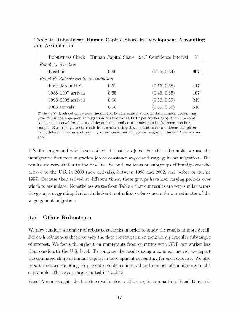
Table 4: Robustness: Human Capital Share in Development Accountingand Assimilation


Panel A: Baseline

Baseline 0.60 (0.55, 0.64) 907

Panel B: Robustness to Assimilation

First Job in U.S. 0.62 (0.56, 0.68) 417

1988–1997 arrivals 0.55 (0.45, 0.65) 167

1998–2002 arrivals 0.60 (0.52, 0.69) 219

2003 arrivals 0.60 (0.55, 0.66) 510Table note: Each column shows the implied human capital share in development accounting(one minus the wage gain at migration relative to the GDP per worker gap); the 95 percentconfidence interval for that statistic; and the number of immigrants in the correspondingsample. Each row gives the result from constructing these statistics for a di↵erent sample orusing di↵erent measures of pre-migration wages, post-migration wages, or the GDP per workergap.

U.S. for longer and who have worked at least two jobs. For this subsample, we use the

immigrant’s first post-migration job to construct wages and wage gains at migration. The

results are very similar to the baseline. Second, we focus on subgroups of immigrants who

arrived to the U.S. in 2003 (new arrivals), between 1998 and 2002, and before or during

1997. Because they arrived at di↵erent times, these groups have had varying periods over

which to assimilate. Nonetheless we see from Table 4 that our results are very similar across

the groups, suggesting that assimilation is not a first-order concern for our estimates of the

wage gain at migration.

4.5 Other Robustness

We now conduct a number of robustness checks in order to study the results in more detail.

For each robustness check we vary the data construction or focus on a particular subsample

of interest. We focus throughout on immigrants from countries with GDP per worker less

than one-fourth the U.S. level. To compare the results using a common metric, we report

the estimated share of human capital in development accounting for each exercise. We also

report the corresponding 95 percent confidence interval and number of immigrants in the

subsample. The results are reported in Table 5.

Panel A reports again the baseline results discussed above, for comparison. Panel B reports

17

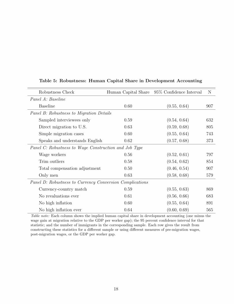
Table 5: Robustness: Human Capital Share in Development Accounting


Panel A: Baseline

Baseline 0.60 (0.55, 0.64) 907

Panel B: Robustness to Migration Details

Sampled interviewees only 0.59 (0.54, 0.64) 632

Direct migration to U.S. 0.63 (0.59, 0.68) 805

Simple migration cases 0.60 (0.55, 0.64) 743

Speaks and understands English 0.62 (0.57, 0.68) 373

Panel C: Robustness to Wage Construction and Job Type

Wage workers 0.56 (0.52, 0.61) 797

Trim outliers 0.58 (0.54, 0.62) 854

Total compensation adjustment 0.50 (0.46, 0.54) 907

Only men 0.63 (0.58, 0.68) 579

Panel D: Robustness to Currency Conversion Complications

Currency-country match 0.59 (0.55, 0.63) 869

No revaluations ever 0.61 (0.56, 0.66) 683

No high inflation 0.60 (0.55, 0.64) 891

No high inflation ever 0.64 (0.60, 0.69) 565Table note: Each column shows the implied human capital share in development accounting (one minus thewage gain at migration relative to the GDP per worker gap); the 95 percent confidence interval for thatstatistic; and the number of immigrants in the corresponding sample. Each row gives the result fromconstructing these statistics for a di↵erent sample or using di↵erent measures of pre-migration wages,post-migration wages, or the GDP per worker gap.

18

the results from a number of checks on the details of migration. We experiment with

including only the immigrants who were sampled (excluding spouses), and including only

those whose first and only migration was to the U.S. The second to last row of Panel B

constrains attention to immigrants with simple immigration histories, meaning that they

had never left their birth country for more than six months before migrating to the U.S.,

and that they worked their last job in their birth country within one year of their first

job in the U.S. The last row shows results for immigrants who report both speaking and

understanding spoken English well or very well. The results throughout are very similar to

the baseline.

Panel C reports the results from a number of robustness checks dealing with the construction

of wages. The first row reports the result using only workers who worked for wages before

and after migrating. The second row reports the results when we trim more potential

outliers, now including anyone who reports less than $0.10 per hour in their birth country,

less than $5.00 per hour in the U.S., or more than $100 per hour in either country. The

third row includes an adjustment to wages for total compensation. The idea is that the pre-

migration wages in poor countries may reflect total payments to labor, whereas wages in the

U.S. do not include benefits. To see whether this might matter, we multiply the reported

U.S. wage by the national average ratio of total compensation to wages and salaries, which

is 1.23, taken from NIPA. The last row includes only men. The results in all cases exceed

one-half.

Panel D reports robustness to the details of currency conversion. We find similar results if

we focus on cases where immigrants report being paid in a currency that “matches” their

country of work, or if we exclude immigrants who report being paid in currencies that have

ever been devalued. Recall that our baseline results already exclude immigrants who were

paid in a currency that has been subsequently devalued. We also find similar results if we

exclude immigrants who were paid in currencies that have subsequently or ever experienced

high inflation.

Across all of these subgroups and robustness checks we find that the human capital share

in development accounting is remarkably consistent, in the range of 0.50–0.64, suggesting

that it is not driven by complicated migration experiences, wage construction, or wage

adjustment. Given that our results are robust, we turn to understanding the relationship

between these results and the literature.

19

5 Selection

In the previous section we measured the importance of human capital for development ac-

counting by comparing the wage gains at migration to the total gap in GDP per worker. As

discussed in Section 2.1, this deals with most common concerns about immigrant selection

because it compares wages earned by a given worker in two di↵erent countries. Nonetheless,

it is of interest to back out the implied degree of selection, which we measure here as the gap

between immigrants’ pre-migration characteristics and the characteristics of non-migrants

in the same country. The patterns and degree of selection are of interest in their own right.

As we show below, they are also useful for understanding why our results di↵er so much

from those in the literature.

5.1 Selection and Wages

We start by measuring the implied extent of selection on wages. In principle, one would

like to compare the pre-migration hourly wage of immigrant i to the mean wage of non-

migrants in the same country, wi,c/wc. Unfortunately, we lack widespread data on pre-

migration wages for many countries; given the high rates of self-employment in many poor

countries, it is not clear whether such a database would even valuable. This leads us to

substitute wc = (1 � ↵c)yc/nc, where nc is the hours worked per worker per year. Gollin

(2002) documents that ↵c does not vary systematically with average income, while Bick et

al. (2015) document that hours worked per employed person do not di↵er much between

the U.S. and poor countries. If we assume that these two factors are roughly constant, we

arrive at a simple measure of selection for an individual:

�i =wi,c/yc

wU.S./yU.S.. (5)

In words, this equation says immigrants are highly selected if the ratio of their pre-migration

wage to PPP GDP per worker is high relative to the benchmark, which is the mean wage

of Americans relative to U.S. PPP GDP per worker.

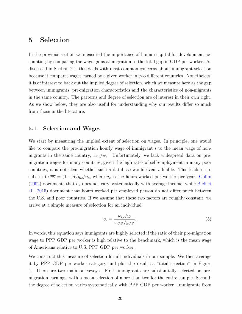
We construct this measure of selection for all individuals in our sample. We then average

it by PPP GDP per worker category and plot the result as “total selection” in Figure

4. There are two main takeaways. First, immigrants are substantially selected on pre-

migration earnings, with a mean selection of more than two for the entire sample. Second,

the degree of selection varies systematically with PPP GDP per worker. Immigrants from

20

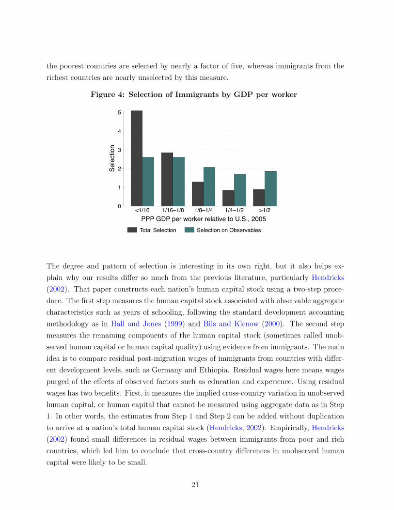
the poorest countries are selected by nearly a factor of five, whereas immigrants from the

richest countries are nearly unselected by this measure.

Figure 4: Selection of Immigrants by GDP per worker

0

1

2

3

4

5Se

lect

ion

<1/16 1/16–1/8 1/8–1/4 1/4–1/2 >1/2PPP GDP per worker relative to U.S., 2005Total Selection Selection on Observables

The degree and pattern of selection is interesting in its own right, but it also helps ex-

plain why our results di↵er so much from the previous literature, particularly Hendricks

(2002). That paper constructs each nation’s human capital stock using a two-step proce-

dure. The first step measures the human capital stock associated with observable aggregate

characteristics such as years of schooling, following the standard development accounting

methodology as in Hall and Jones (1999) and Bils and Klenow (2000). The second step

measures the remaining components of the human capital stock (sometimes called unob-

served human capital or human capital quality) using evidence from immigrants. The main

idea is to compare residual post-migration wages of immigrants from countries with di↵er-

ent development levels, such as Germany and Ethiopia. Residual wages here means wages

purged of the e↵ects of observed factors such as education and experience. Using residual

wages has two benefits. First, it measures the implied cross-country variation in unobserved

human capital, or human capital that cannot be measured using aggregate data as in Step

1. In other words, the estimates from Step 1 and Step 2 can be added without duplication

to arrive at a nation’s total human capital stock (Hendricks, 2002). Empirically, Hendricks

(2002) found small di↵erences in residual wages between immigrants from poor and rich

countries, which led him to conclude that cross-country di↵erences in unobserved human

capital were likely to be small.

21

The second advantage of focusing on residual wages is that they help account for the fact

that immigrants are selected on observable proxies for human capital. To understand the

underlying assumption on selection, consider two workers i and i0 who were born in c and

c0 and now working in the U.S. The main idea is to compare their residual wages wi,c,U.S.

and wi0,c0,U.S to the gap in GDP per worker:

log(wi,c,U.S.)� log(wi0,c0,U.S.)

log(yc)� log(yc0)=

log(hi)� log(hi0)

log(yc)� log(yc0)

⌘ log(hc)� log(hc0) + log(�i)� log(�i0)

log(yc)� log(yc0)

The first equality follows from the same assumptions made in this paper, which allow one

to translate di↵erences in wages to di↵erences in human capital stocks. In the second line

we define �i ⌘ hi/hc as selection on unobservables, which is the ratio of residual (non-

observable) human capital of individual i to the residual (non-observable) human capital

of the average non-migrant in c. The object of interest is the variation in average residual

(non-observable) human capital with respect to GDP per worker. This can be measured

using only immigrants’ post-migration wages if immigrants from countries at di↵erent de-

velopment levels are equally selected on unobserved characteristics (log(�i) independent of

log(y)). Given our data, we can test this assumption.

To do so, we construct a measure of residual wages and selection along the lines of Hendricks

(2002). The details are in Appendix B, but the basic idea is to use a log-wage regression

on a sample of natives to estimate the e↵ect of observable characteristics, in this case age

and education. We do so using the 2003–04 ACS, which is a large representative sample

that closely matches the time frame of the NIS. We construct a measure of selection on

observable characteristics by valuing the di↵erence in age and education of immigrants

and non-migrants with the estimated coe�cients. Our data on the characteristics of non-

migrants come from Barro and Lee (2013), who give the educational attainment and age

composition of the population for most countries worldwide.

The results of this exercise, averaged by PPP GDP per worker group, are labeled as selection

on observables in Figure 4. This measure does capture a fair amount of selection, around

a factor of two on average. However, it is much less variable across GDP groups than is

our measure of total selection; whereas total selection varies between a factor of 0.8 and

4.6, selection on observables varies between only a factor of 1.7 and 2.6. It follows that

there is a strong relationship between selection on unobserved characteristics and GDP

22

per worker. This fact is key to the di↵erence between our paper and Hendricks (2002).

Our interpretation is that the small gap in residual wages between poor and rich country

immigrants is due in part to stronger selection of poor country immigrants on unobserved

characteristics.12

5.2 Selection and Wages: A Microdata Approach

Given the preceding discussion, it is clear that the key reason why our results di↵er from the

previous literature is that we are finding substantial selection of immigrants, particularly

those from poor countries. A key question is whether this substantial degree of selection is

plausible, or whether the results may be driven by, say, measurement error or recall bias.

We undertake two additional exercises to speak to these concerns.

In the first, we construct an alternative measure of selection by comparing immigrants’ pre-

migration outcomes to those of non-migrants using microdata. We focus on India because

there are many Indian immigrants in the NIS; because those immigrants are measured to

be highly selected; and because we have access to nationally representative microdata with

wages, the 1999 Indian Socio-Economic Survey.13 We limit our attention to immigrants

whose last pre-migration job was in India and who were paid in rupees between 1995 and

2003. For this sample, the degree of selection implied by equation (5) is substantial: a factor

of 5.25, much larger than the typical poor country (see Figure 4). We adjust the reported

pre-migration wage to a year-1999 equivalent by deflating at the rate of nominal GDP per

worker growth, taken from the Penn World Tables. After doing so, we can directly measure

selection by comparing the mean pre-migration wage of immigrants to the mean wage of

non-migrants, which yields a very similar estimate of selection, a factor of 5.97. This fact

o↵ers support for the approximations used in equation (5).

Our goal is to think about whether this degree of selection is plausible. To do so, we ask

how much of it can be accounted for by the observable characteristics of the worker, as

in the previous subsection. Since we have access to Indian microdata, we can account for

a broader set of characteristics and use the prevailing returns to those characteristics in

India, not the U.S. We focus on four sets of characteristics: sex, education, experience, and

occupation. We regress log hourly wages in India on dummies for sex, education (in seven

12The quantitative importance of unobserved characteristics is also a di↵erence between our work andthat of Clemens et al. (2008), who use estimates of wages by observed characteristics to estimate the gapin marginal products across countries. The key assumption behind this methodology is that the meanunobserved human capital of non-migrants is the same across countries.

13For details see Appendix B.2.

23

categories, as in Barro and Lee (2013)), and occupation, as well as a quartic in potential

experience. We then match these coe�cients to workers in the NIS. For the most part the

mapping is straightforward, but we do have to construct our own crosswalk between India’s

detailed occupational coding scheme and the NIS coding scheme. After doing so, we can

predict for each worker the wage we would expect them to earn in the Indian Census based

on their characteristics.

We find that the mean expected wage (based on observed characteristics) is 29 rupees per

hour, whereas the actual reported pre-migration wage is 64 rupees. This implies that the

factor 5.97 selection can be partitioned into a factor of 2.40 selection on observable char-

acteristics and a factor 2.18 selection on unobservable characteristics. Thus, the majority

of selection can be understood especially as selection on occupation and education.14 We

can go even further in understanding selection if we utilize the work of Commander et al.

(2008), who surveyed a number of large Indian software firms about their business. Among

other information, they note that mean annual earnings paid for software developers by

these firms was 223,000 rupees in 1999. Assuming developers work 40–50 hours per week,

50 weeks per year, this corresponds to an hourly wage of 89–112 rupees per hour, which is

more than double the overall mean wage for programmers from the Indian Census. This

information is useful because a large majority of Indian immigrants in our sample report

some variant of computer programming as their pre-migration occupation. It suggests that

much of the remaining selection can likely be attributed to the fact that Indian migrants

were likely employed in the large, skill-intensive firms with the connections and knowledge

to secure visas for their employees.

We acknowledge that the specifics of this finding are unlikely to generalize to immigrants

from other countries. Nonetheless, we find it instructive that for one of the most selected

countries in our sample, we can plausibly explain the pre-migration wage gap using infor-

mation on education, occupation, and employer, which in turn suggests that we do not need

to appeal to measurement error or recall bias. We now turn to a more general investigation.

5.3 Selection on Other Characteristics

Our second approach to thinking about the plausibility of strong selection for poor country

immigrants is to study selection on non-wage dimensions. For example, immigrants from

the poorest group have on average 13.0 years of schooling. 32 percent have a college degree

14To put the selection on unobservables into context, a factor of 2.18 above the mean puts immigrantsat the 91st percentile of the distribution of residual wages.

24

while only 17 percent have not graduated from high school. This finding is similar to what

is reported in Schoellman (2012), namely that immigrants from poor countries are much

more educated than non-migrants born in the same country.

We also study the characteristics of workers’ pre-migration jobs. We again find that they

are consistent with strong selection. First, 77 percent of immigrants from the poorest

countries were employed for wages in their pre-migration job. This fact stands at odds with

the general prevalence of self-employment in poor countries. Second, we study occupation

as reported in 25 broad groupings. Of these 25, the three most commonly reported are

o�ce and administrative support; sales and related; and management. They account for

45 percent of all the pre-migration occupations. On the other hand, not a single immigrant

in the poorest group reports having previously worked in agriculture, despite the fact that

this occupation accounts for the majority of employment in most poor countries (Restuccia

et al., 2008). We conclude that there is ample evidence that immigrants from the poorest

countries are extremely selected on their pre-migration labor market experiences.

6 Skill Transferability

Our baseline estimates measure the importance of country by comparing the pre- and post-

migration wages of a fixed individual. If immigrants are able to use their human capital

equally in the two countries, then the gap in wages is entirely determined by country-specific

factors. However, a common concern with immigrants is that their skills may not transfer

perfectly when they migrate. This could happen either if skills are heterogeneous and they

have acquired skills that are not highly valued in the U.S., or if skills are homogeneous but

barriers such as accreditation, licensure, or discrimination prevent them from fully utilizing

their skills.

The first goal of this section is to provide evidence on skill transferability by comparing

immigrants’ pre- and post-migration occupations. We document that occupational switch-

ing is widespread and that most immigrants move to lower-paying jobs, which is a possible

sign of imperfect skill transfer. We then consider the importance of this finding for our

development accounting results. In Appendix D.2 we provide a simple model to formalize

the following intuition: if immigrants have skills but cannot use them in the U.S., then this

depresses their post-migration wage and our estimated wage gains at migration. It then

follows that we understate the role of country and overstate the role of human capital in

development accounting. We show that conservative corrections for skill transfer push our

25

Table 6: Occupational Changes at Migration

GDP category Occupational Switch Mean Change

Lower-Paying Same Occupation Higher-Paying

<1/16 68% 7% 25% -14%

1/16–1/8 60% 18% 22% -15%

1/8–1/4 65% 8% 28% -15%

1/4–1/2 65% 9% 26% -17%

>1/2 47% 30% 23% 0%Table note: Columns give the fraction of immigrants who switched to lower-paying jobs, stayed atthe same job, or switched to higher-paying jobs at migration, as well as the average change in jobpay at migration, where average pay is measured using mean wage of natives. Rows give thoseresults for di↵erent PPP GDP per worker groups.

estimate of the human capital share down towards one-half.

6.1 Evidence on Skill Transferability

We measure skill transfer by comparing immigrants’ pre- and post-migration occupations.15

Measuring skill transferability through occupational changes is subject to two biases that

push in opposite directions and are not easy to quantify. On the one hand, we are assuming

that immigrants who do not practice their pre-migration occupation do so because of a lack

of skill transferability, ruling out a lack of skill altogether, e.g., that they may simply have

been unqualified. On the other hand, our measure does not capture within-occupation

skill loss. For example, we capture doctors who are forced to work as taxi drivers, but

not specialized doctors forced to work as family doctors. However, we note that the NIS

uses the 2000 U.S. Census occupation codes, which includes over 450 possible occupational

choices. With these two caveats in mind, we now turn to analyzing occupational switches.16

We begin by examining the frequency of occupational switches. We focus on the detailed

occupational coding scheme, which includes roughly 450 categories. We find that most

immigrants switch jobs after migrating. The fraction staying in the same occupation is given

in column 3 of Table 6 and ranges from 7–30% depending on the level of development. This

15The literature on the economics of immigration has explored several ways to measure skill transfer. Ourapproach and findings parallel those of Chiswick et al. (2005) and especially Akresh (2008), who also usesthe NIS. Chiswick and Miller (2009) employs an alternative strategy of comparing immigrants’ educationto that of natives in the same occupation, using “overeducation” as a proxy for imperfect skill transfer.

16We have also explored repeating all this analysis using industry data and find similar results throughout.

26

figure is driven mostly by changes to entirely new occupations; only 12–46% of immigrants

work even in the same broad occupational category after migrating (not shown).

A change in occupation does not indicate whether the new occupation is better or worse

than the old occupation. As a proxy for the “quality” of an occupation, we construct the

mean wage of natives for that occupation from the 2003–04 American Community Survey

(ACS).17 We merge this mean wage by occupation with both the pre- and post-migration

occupations of immigrants in the NIS. This procedure provides us with a quantitative

ranking of each immigrant’s pre- and post-migration occupation and hence a measure of

the extent to which an immigrant’s new job is better or worse than their old one. For

example, take an immigrant who worked as a physician in his or her birth country but

works as a taxi driver in the U.S. Based on the observation that the mean wage of taxi

drivers in the U.S. is $9.52 while the mean wage of physicians is $38.71, we would infer that

the immigrant’s occupational switch involved a downgrade. The extent of the change in

mean wages (75 percent) provides a metric to suggest that the occupational downgrading

was significant.

The remaining columns of Table 6 give a sense of the distribution and average change in

occupation at arrival. Roughly two-thirds of immigrants move to lower-paying jobs after

migrating, while only one-quarter move to higher-paying jobs, except for the highest GDP

per worker group. The mean change in occupation quality (again, judged by mean native

wage) is a loss of 14–17 percent upon migration. Only immigrants from the richest countries

report no occupational downgrading at migration. One interpretation of this finding is that

most immigrants cannot perfectly transfer their skills to the U.S.

6.2 Development Accounting with Imperfect Skill Transfer

If we interpret these findings as evidence of imperfect skill transfer, then they have impor-

tant implications for our development accounting results. We explore this idea further in

two ways, focusing throughout on immigrants from countries with less than one-fourth of

US GDP p.w. First, we check the robustness of our results to focusing on groups for whom

skill transfer is likely less of a problem. There are two main groups in the NIS: immigrants

who entered the U.S. on employment visas; and those who work the same detailed occu-

pation before and after migrating. The implied development accounting results for these

subsamples are shown along with the baseline in Table 7. While human capital accounts

17See Appendix B for details.

27

Table 7: Development Accounting and Skill Transfer

Robustness Check Human Capital Share 95% C.I.

Baseline 0.60 (0.55, 0.64)

Employment visa 0.52 (0.46, 0.59)

Same narrow occupation 0.56 (0.49, 0.63)

Skill transfer: mean wage 0.46 (0.42, 0.50)Table note: Each column shows the implied human capital share in development accounting(one minus the wage gain at migration relative to the GDP per worker gap) and the 95 percentconfidence interval. Each row gives the result from constructing these statistics for a di↵erentsample or using di↵erent measures of post-migration wages.

for 60 percent of cross-country income di↵erences in the baseline, it accounts for a modestly

lower 52–56 percent when focusing in these subsamples.

As a second check, we consider imputing to immigrants a higher wage if they experienced

occupational downgrading. This step is logical if the main reason for occupational down-

grading is artificial barriers such as licensure rather than a lack of skills among immigrants.

By increasing the post-migration wage of immigrants we also increase the implied wage

gains at migration and lower the implied human capital share for development accounting.

We implement this idea by adding to each downgraded immigrant’s wage the gap in mean

native wages between their pre- and post-migration occupations. For example, take an

immigrant who reports having been a doctor before arriving to the U.S., but who is now

a taxi driver earning $8 an hour. We would add to this wage the di↵erence between the

mean native wage of doctors and taxi drivers, which is $29.19, resulting in a total wage of

$37.17. The resulting adjustment is substantial, increasing the mean post-migration wage

of immigrants by 39 percent. We then re-compute wage gains at migration and the human

capital share in development accounting. The results are reported in the last row of Table 7.

We find that human capital in this case would account for just under half of cross-country

income di↵erences.

There are two main take-aways from this section. First, most immigrants switch to lower-

paying occupations when they immigrate to the U.S. If this fact is interpreted as the result of

imperfect skill transfer, then our baseline results overstate the importance of human capital

for development accounting. We conduct several checks that suggest that correcting for this

could lower the human capital share to 46–56 percent, still much larger than the standard

result in the literature. On the other hand, if occupational downgrading indicates a lack of

skills, then the baseline result of 60 percent is appropriate.

28

7 Elasticity of Substitution Across Skill Types

Our estimates so far have all followed the precedent of the accounting literature by assuming

that workers of di↵erent skill levels are perfect substitutes in the aggregate production

function. Some recent work has noted that this assumption is important for a number of

development questions (Roys and Seshadri, 2014; Caselli and Coleman, 2006). The most

directly related work is Jones (2014), who notes that development accounting results are

very sensitive to it. Even modest reductions of the elasticity of substitution (from infinity)

can substantially increase the role for human capital in accounting for cross-country income

di↵erences. At the same time, there is relatively little evidence on the long-run or cross-

country elasticity of substitution. The best-known estimate spans the U.S. from 1950–1990,

but there is no guarantee that a similar estimate applies to the much poorer countries in

our sample (Ciccone and Peri, 2005).

Our insight is that the wage gains of immigrants to the U.S. can be informative about the

elasticity of substitution. We formalize this idea in Appendix D.3, but the intuition is as

follows. In a model with imperfect substitution, the wage gains of immigrants depend on

country-specific factors such as the capital-output ratio and TFP, but also on the di↵erence

in the relative supply of skilled and unskilled labor between the immigrant’s birth country

and the U.S. Educated immigrants from poor countries should gain less than uneducated

immigrants because while educated immigrants move to a country where educated labor

is relatively more common, uneducated immigrants move to a country where uneducated

labor is relatively less common. Hence we can use the relative wage gains of immigrants with

di↵erent education levels as evidence on the elasticity of substitution between education

groups.

To implement this idea, we focus again on immigrants from countries with PPP GDP per

worker less than one-quarter the U.S. level. We measure education by combining data on

degree attainment and years of schooling, giving preference to the former where available.

We then break workers into four groups: those with less than a high school degree (or

less than twelve years of schooling); those with exactly a high school degree (or twelve

years of schooling); those with some college but not a bachelor’s degree (or 13–15 years of

schooling); and those with a bachelor’s degree or more (or 16 or more years of schooling).

In the context of development it would be interesting to further subdivide the less than

high school group: perhaps the important margin of substitution is between those with no

schooling versus some, or primary versus secondary. The small sample size of the less than

high school group prevents us from exploring this further.

29

Figure 5 shows the pre-migration wage, post-migration wage, and wage gain at migration

by education group. We find little variation in pre- or post-migration wages among the

first three groups, whereas college graduates earn more both before and after migration.

In terms of wage gains, however, we find very similar results for each of the groups of

immigrants.

Figure 5: Wages and Education Level


0

5

10

15

20

25

Hou

rly W

age,

200

3 U

S D

olla

rs

<HS HS SC CDEducation Level



0

1

2

3

4

Rat

io o

f Pos

t to

Pre–

Mig

ratio

n W

age

<HS HS SC CDEducation Level

The corresponding development accounting results are given in Table 8. We find no strong

support for imperfect substitution: the proportional wage gains are roughly the same for all

workers with at least a high school degree, and are lower for high school dropouts, whereas

a theory with imperfect substitution would predict that it is higher. Indeed, it is apparent

from our confidence intervals that we cannot reject that the wage change is the same across

groups, implying that we cannot reject the case of perfect substitutes.18

8 Conclusion

In this paper we use data on pre- and post-migration outcomes of immigrants along with

an extended development accounting framework to infer the importance of human capital

18The framework Caselli and Coleman (2006) o↵ers an alternative interpretation of these facts. There,educated and uneducated workers are imperfect substitutes, but countries operate technologies with di↵er-ent weights on educated and uneducated labor. In this case immigrants would be moving between countrieswith di↵erent relative supplies of and demand for educated labor; the lack of correlation between wage gainsand education could simply reflect that those two forces roughly o↵set.

30

Table 8: Robustness: Human Capital Share in Development Accounting byEducation


Less than High School Graduate 0.50 (0.39, 0.61) 138

High School Graduate 0.58 (0.48, 0.68) 183

Some College, No Degree 0.50 (0.35, 0.64) 82

College Degree or More 0.66 (0.61, 0.71) 504Table note: Each column shows the implied human capital share in development accounting (one minusthe wage gain at migration relative to the GDP per worker gap); the 95 percent confidence interval forthat statistic; and the number of immigrants in the corresponding sample. Each row gives the resultfrom constructing these statistics for the baseline sample or for subsamples with the di↵erent levels ofeducation.

versus country in accounting for cross-country income di↵erences. Our key finding is that

immigrants’ wage gains at migration are small relative to gaps in PPP GDP per worker. We

infer that human capital accounts for 60 percent of cross-country income di↵erences. We

conduct a range of robustness checks and find this figure to be robust. Our result is much

larger than those in the previous literature because it provides a direct way to measure and

control for selection, which we find to be large and strongly correlated with development.

We also provide novel evidence on two issues frequently raised in the literature. First, we

find that immigrants’ experiences are consistent with the assumption of perfect substitu-

tion across labor types. The key finding here is that immigrants with di↵erent education

levels have similar wage gains at migration, which is inconsistent with imperfect substi-

tution. Second, we study skill transfer through immigrants’ changes in occupation. We

find evidence that immigrants move to lower-paying occupations upon arrival. We provide

calculations to show that reasonable corrections for this possible imperfect skill transfer

lower the human capital share in development accounting to roughly one-half.

31

References

Akresh, Ilana Redstone, “Occupational Trajectories of Legal U.S. Immigrants: Down-

grading and Recovery,” Population and Development Review, 2008, 34 (3), 435–456.

Barro, Robert J and Jong Wha Lee, “A new data set of educational attainment in

the world, 1950–2010,” Journal of Development Economics, 2013, 104, 184–198.

Bick, Alex, Nicola Fuchs-Schundeln, and David Lagakos, “How Do Average Hours

Worked Vary With Development? Cross Country Evidence and Implications,” October

2015. mimeo, Arizona State University.

Bils, Mark and Peter J. Klenow, “Does Schooling Cause Growth?,” American Eco-

nomic Review, December 2000, 90 (5), 1160–1183.

Borjas, George J., “Self-Selection and the Earnings of Immigrants,” American Economic

Review, September 1987, 77 (4), 531–553.

Caselli, Francesco, “Accounting for Cross-Country Income Di↵erences,” in Philippe

Aghion and Steven N. Durlauf, eds., Handbook of Economic Growth, Vol. 1A, Elsevier,

2005, chapter 9, pp. 679–741.

Caselli, Franco and Wilbur John Coleman II, “The World Technology Frontier,”

American Economic Review, June 2006, 96 (3), 499–522.

Chiswick, Barry R and Paul W Miller, “The international transferability of immi-

grants human capital,” Economics of Education Review, 2009, 28 (2), 162–169.

, Yew Liang Lee, and Paul W Miller, “A longitudinal analysis of immigrant oc-

cupational mobility: A test of the immigrant assimilation hypothesis,” International

Migration Review, 2005, 39 (2), 332–353.

Ciccone, Antonio and Giovanni Peri, “Long-run substitutability between more and

less educated workers: evidence from US states, 1950–1990,” Review of Economics and

Statistics, 2005, 87 (4), 652–663.

Clemens, Michael A, “Why do programmers earn more in Houston than Hyderabad?

Evidence from randomized processing of US visas,” The American Economic Review,

2013, 103 (3), 198–202.

32

, Claudio E Montenegro, and Lant Pritchett, “The place premium: wage di↵erences

for identical workers across the US border,” 2008. World Bank Policy Research Working

Paper No. 4671.

Commander, Simon, Rupa Chanda, Mari Kangasniemi, and L Alan Winters,

“The Consequences of Globalisation: India’s Software Industry and Cross-border Labour

Mobility1,” The World Economy, 2008, 31 (2), 187–211.

Cordoba, Juan Carlos and Marla Ripoll, “What Explains Schooling Di↵erences Across

Countries?,” Journal of Monetary Economics, March 2013, 60 (2), 184–202.

Cubas, German, B Ravikumar, and Gustavo Ventura, “Talent, labor quality, and

economic development,” Review of Economic Dynamics, forthcoming.

Duleep, Harriet Orcutt, “The Adjustment of Immigrants in the Labor Market,” in

Barry R. Chiswick and Paul W. Miller, eds., Handbook of the Economics of International

Migration, Elsevier, 2015, chapter 3, pp. 105–182.

Erosa, Andres, Tatyana Koreshkova, and Diego Restuccia, “How Important is

Human Capital? A Quantitative Theory Assessment of World Income Inequality,” Review

of Economic Studies, October 2010, 77 (4), 1421–1449.

Gibson, John, David McKenzie, Halahingano Rohorua, and Steven Stillman,

“The Long-Term Impacts of International Migration: Evidence from a Lottery,” Novem-

ber 2015. World Bank Policy Research Working Paper 7495.

Gollin, Douglas, “Getting Income Shares Right,” Journal of Political Economy, April

2002, 110 (2), 458–474.

Hall, Robert E. and Charlies I. Jones, “Why Do Some Countries Produce So Much

More Output Per Worker Than Others?,” Quarterly Journal of Economics, February

1999, 114 (1), 83–116.

Hanushek, Eric A and Ludger Woessmann, “Do Better Schools Lead to More Growth?

Cognitive Skills, Economic Outcomes, and Causation,” Journal of Economic Growth,

2012, 17 (4), 267–321.

Hendricks, Lutz, “How Important Is Human Capital for Development? Evidence from

Immigrant Earnings,” American Economic Review, March 2002, 92 (1), 198–219.

33

Heston, Alan, Robert Summers, and Bettina Aten, Penn World Table Version 6.1,

Center for International Comparisons of Production, Income and Prices at the University

of Pennsylvania, October 2002.

, , and , Penn World Table Version 6.2, Center for International Comparisons of

Production, Income and Prices at the University of Pennsylvania, September 2006.

, , and , Penn World Table Version 7.1, Center for International Comparisons of

Production, Income and Prices at the University of Pennsylvania, November 2012.

, , and , Penn World Table, Center for International Comparisons of Production,

Income and Prices at the University of Pennsylvania.

Hsieh, Chang-Tai and Peter J Klenow, “Development accounting,” American Eco-

nomic Journal: Macroeconomics, 2010, 2 (1), 207–223.

Jasso, Guillermina, Douglas S. Massey, Mark R. Rosenzweig, and James P.

Smith, “The U.S. New Immigrant Survey: Overview and Preliminary Results Based on

the New-Immigrant Cohorts of 1996 and 2003,” in Beverley Morgan and Ben Nicholson,

eds., Immigration Research and Statistics: Service workshop on longitudinal surveys and

cross-cultural survey design. Workshop proceedings., London: Crown Publishing, 2005.

, , , and , “The New Immigrant Survey.” A research project funded by NIH

HD33843, NSF, USCIS, ASPE & Pew. Restricted Use Data, Version 1 August 2007.

Retrieved February 2014. Persons interested in obtaining NIS Restricted Use Data should

see http://nis.princeton.edu/data_restricted.html for further information.

Jones, Benjamin F., “The Human Capital Stock: A Generalized Approach,” American

Economic Review, November 2014, 104 (11), 3752–77.

Kennan, John, “Open borders,” Review of Economic Dynamics, 2013, 16 (2), L1–L13.

King, Miriam, Steven Ruggles, J. Trent Alexander, Sarah Flood, Katie

Genadek, Matthew B. Schoreder, Brandon Trampe, and Rebecca Vick, “Inte-

grated Public Use Microdata Series, Current Population Survey: Version 3.0 [Machine-

readable database],” Minneapolis, MN: Minnesota Population Center [producer and dis-

tributor] 2010. Available online at http://usa.ipums.org/cps/.

Klein, Paul and Gustavo Ventura, “Productivity di↵erences and the dynamic e↵ects

of labor movements,” Journal of Monetary Economics, 2009, 56 (8), 1059–1073.

34

Klenow, Peter J. and Andres Rodriguez-Clare, “The Neoclassical Revival in Growth

Economics: Has It Gone Too Far?,” in Ben S. Bernanke and Julio J. Rotemberg, eds.,

NBER Macroeconomics Annual 1997, The MIT Press, 1997, pp. 73–103.

Lagakos, David, Ben Moll, Tommaso Porzio, Nancy Qian, and Todd Schoellman,

“Life-Cycle Wage Growth Across Countries,” 2015. mimeo, UCSD.

Lubotsky, Darren, “Chutes or Ladders? A Longitudinal Analysis of Immigrant Earn-

ings,” Journal of Political Economy, 2007, 115 (5), 820–867.

Manuelli, Rodolfo E. and Ananth Seshadri, “Human Capital and the Wealth of

Nations,” American Economic Review, 2014, 104 (9), 2736–2762.

McKenzie, David, Steven Stillman, and John Gibson, “How important is selection?

experimental vs. non-experimental measures of the income gains from migration,” Journal

of the European Economic Association, 2010, 8 (4), 913–945.

Minnesota Population Center, “Integrated Public Use Microdata Series — Interna-

tional: Version 6.3 [Machine-readable database].,” Minneapolis: University of Minnesota.

2014. http://www.ipums.org.

Restuccia, Diego, Dennis T Yang, and Xiaodong Zhu, “Agriculture and Aggregate

Productivity: A Quantitative Cross-Country Analysis,” Journal of Monetary Economics,

March 2008, 55 (2), 234–250.

Rosenzweig, Mark R, “Global wage inequality and the international flow of migrants,”

January 2010. Yale University Economic Growth Center Discussion Paper no. 983.

Roys, Nicolas and Ananth Seshadri, “Economic development and the organization of

production,” October 2014. mimeo, University of Wisconsin–Madison.

Ruggles, Steven, Trent J. Alexander, Katie Genadek, Ronald Goeken,

Matthew B. Schoreder, and Matthew Sobek, “Integrated Public Use Microdata

Series: Version 5.0 [Machine-readable database],” Minneapolis, MN: Minnesota Popu-

lation Center [producer and distributor] 2010. Available online at http://usa.ipums.

org/usa/.

Schoellman, Todd, “Education Quality and Development Accounting,” Review of Eco-

nomic Studies, 2012, 79 (1), 388–417.

35

, “Refugees and Early Childhood Human Capital,” American Economic Journal: Macroe-

conomics, forthcoming.

Weil, David N, “Accounting for the e↵ect of health on economic growth,” The Quarterly

Journal of Economics, 2007, 122 (3), 1265–1306.

World Bank, World Development Indicators, Washington D.C.: World Bank, 2014.

36

Online Appendices: Not for Publication

A New Immigrant Survey Details

The NIS attempted to sample 12,500 adult immigrants sampled from government records

between June 2003 and June 2004. They were able to do so in 68.6 percent of cases.

Surveyors also collected detailed data on the spouse of the interviewee. In many cases the

spouse was also an immigrant; in such cases, we include the spouse in our sample, although

we show in the text that this is not important for our main results. We utilize the restricted

version of the data, which allows us to identify the exact country of birth and work, rather

than broad geographic regions.

The goal of this appendix is to show how the various adjustments and sample restrictions

a↵ect the overall sample size for the results used in the paper. The figures throughout are

summarized in Table A1. The first row shows the initial sample size of workers for whom we

can construct pre-migration hourly wage, post-migration hourly wage, or both (necessary

for computing the wage gains at migration). While we have 4,700–5,700 workers with wages

before or after migration, we only have both for around 2,300 workers. The main reason for

the disparity is that many of our immigrants did not work before immigrating or are not

working at the time of the survey. Roughly 60 percent of immigrants with post-migration

wages but no pre-migration report never working before immigrating; roughly 75 percent

of immigrants with pre-migration wages but no post-migration wage report that they are

not working. The remaining cases are typically those who work but do not report the

information needed to construct hourly wage, such as income, hours worked, currency in

which they were paid, and so on.

The subsequent rows show the e↵ects on sample size of the various restrictions and adjust-

ments we make. In order: we need to be able to identify the immigrant’s previous country

of work or birth; we need to be able to adjust the wage to PPP-adjusted U.S. dollars;

we need to able to measure the PPP-adjusted GDP per worker in their birth country; we

exclude immigrants who report wages with subsequent devaluations; we trim outliers in the

wage distribution; we focus on immigrants who arrive during or after 1983; and we exclude

anyone who reports having had some U.S. education. The most important restrictions in

terms of lost sample size are being able to adjust wages, excluding immigrants who were

paid in currencies that were subsequently devalued, and excluding immigrants with some

U.S. schooling; each reduces the sample by 200–300 immigrants.

37

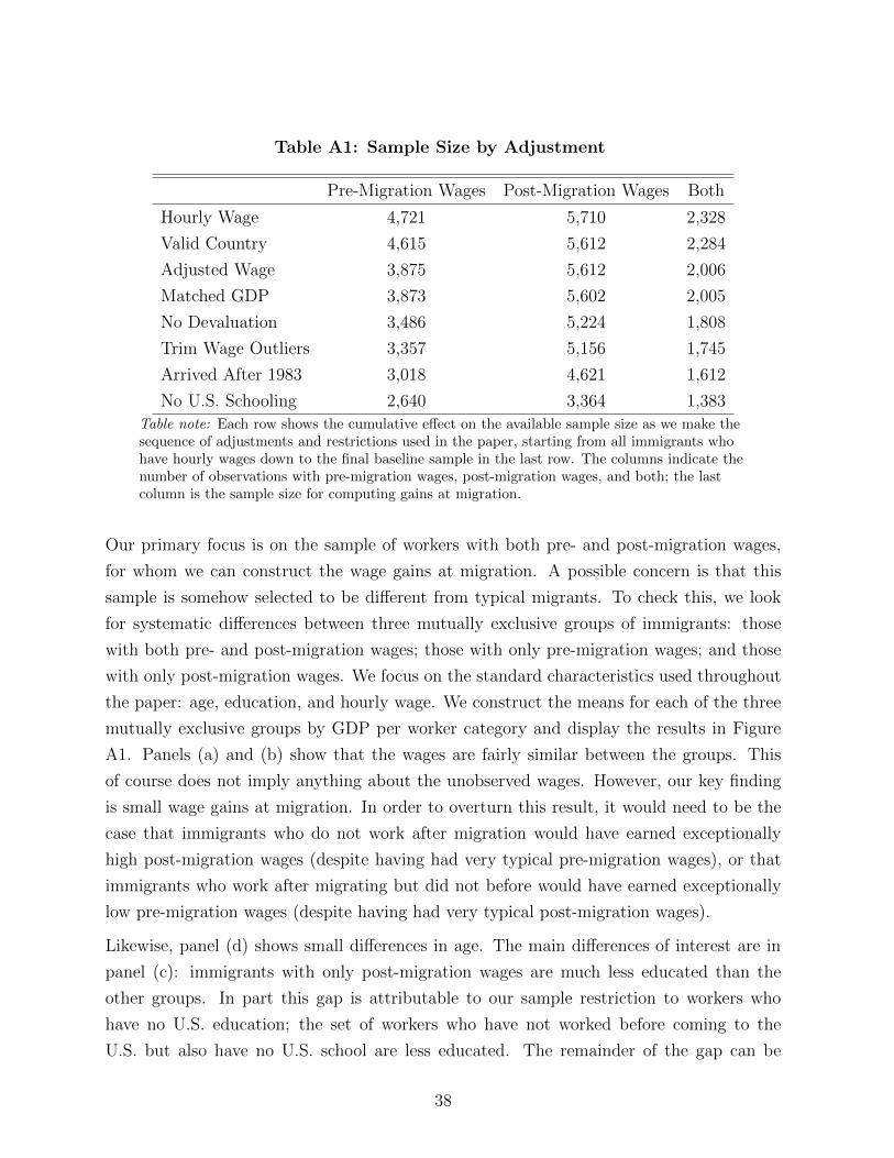
Table A1: Sample Size by Adjustment

Pre-Migration Wages Post-Migration Wages Both

Hourly Wage 4,721 5,710 2,328

Valid Country 4,615 5,612 2,284

Adjusted Wage 3,875 5,612 2,006

Matched GDP 3,873 5,602 2,005

No Devaluation 3,486 5,224 1,808

Trim Wage Outliers 3,357 5,156 1,745

Arrived After 1983 3,018 4,621 1,612

No U.S. Schooling 2,640 3,364 1,383Table note: Each row shows the cumulative e↵ect on the available sample size as we make thesequence of adjustments and restrictions used in the paper, starting from all immigrants whohave hourly wages down to the final baseline sample in the last row. The columns indicate thenumber of observations with pre-migration wages, post-migration wages, and both; the lastcolumn is the sample size for computing gains at migration.

Our primary focus is on the sample of workers with both pre- and post-migration wages,

for whom we can construct the wage gains at migration. A possible concern is that this

sample is somehow selected to be di↵erent from typical migrants. To check this, we look

for systematic di↵erences between three mutually exclusive groups of immigrants: those

with both pre- and post-migration wages; those with only pre-migration wages; and those

with only post-migration wages. We focus on the standard characteristics used throughout

the paper: age, education, and hourly wage. We construct the means for each of the three

mutually exclusive groups by GDP per worker category and display the results in Figure

A1. Panels (a) and (b) show that the wages are fairly similar between the groups. This

of course does not imply anything about the unobserved wages. However, our key finding

is small wage gains at migration. In order to overturn this result, it would need to be the

case that immigrants who do not work after migration would have earned exceptionally

high post-migration wages (despite having had very typical pre-migration wages), or that

immigrants who work after migrating but did not before would have earned exceptionally

low pre-migration wages (despite having had very typical post-migration wages).

Likewise, panel (d) shows small di↵erences in age. The main di↵erences of interest are in

panel (c): immigrants with only post-migration wages are much less educated than the

other groups. In part this gap is attributable to our sample restriction to workers who

have no U.S. education; the set of workers who have not worked before coming to the

U.S. but also have no U.S. school are less educated. The remainder of the gap can be

38

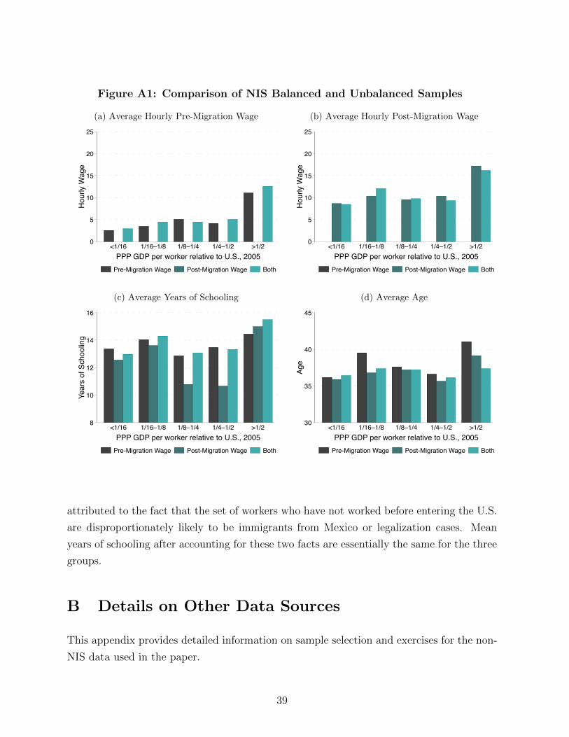
Figure A1: Comparison of NIS Balanced and Unbalanced Samples

(a) Average Hourly Pre-Migration Wage

0

5

10

15

20

25

Hou

rly W

age


Pre-Migration Wage Post-Migration Wage Both

(b) Average Hourly Post-Migration Wage

0

5

10

15

20

25

Hou

rly W

age



(c) Average Years of Schooling

8

10

12

14

16

Year

s of

Sch

oolin

g



(d) Average Age

30

35

40

45

Age



attributed to the fact that the set of workers who have not worked before entering the U.S.

are disproportionately likely to be immigrants from Mexico or legalization cases. Mean

years of schooling after accounting for these two facts are essentially the same for the three

groups.

B Details on Other Data Sources

This appendix provides detailed information on sample selection and exercises for the non-

NIS data used in the paper.

39

B.1 American Community Survey

At several points in the paper we use the American Community Survey (ACS) as a bench-

mark for our NIS results. We focus on the 2003–04 ACS, which combine to form a nationally

representative sample of slightly less than one percent of the U.S. population surveyed in

the same years as the NIS.19 We focus on a standard sample of employed wage workers

aged 16-70. We construct hourly wages using annual labor income, usual hours worked per

week, and weeks worked in the previous year. We code the reported educational attainment

codes into years of schooling in line with standard practice.

We study two groups in the ACS. The first is natives, defined as individuals born in the

U.S. or its territories. The second is immigrants, defined as individuals born outside the

U.S. or its territories. For immigrants we further restrict the sample to exclude workers

with imputed wages or who are likely to have completed some schooling inside the U.S.,

which is based on reported schooling and the year of immigration.

Most of the results (such as mean native wages by occupation) are fairly straightforward,

particularly since the NIS and the ACS use the occupation and industry coding schemes.

The lone exception is the facts about residual wages of immigrants. To construct residual

wages, we first run a standard wage regression using only natives, where log hourly wage

is regressed on five year age bins (15–19, 20–24, .. 65+), a gender dummy, and years of

schooling. An immigrant’s residualized wage is then their log-wage net of the predicted

wage from this regression.

B.2 Indian Socio-Economic Survey

Micro data for India are taken from the 1999 Socio-Economic Survey (retrieved from

IPUMS-I (Minnesota Population Center, 2014)). The sample contains full time (FULL-

TIME = 2) wage workers (CLASSWRK = 2) between the ages of 18 and 65. We require

information on schooling (EDATTAIND), wage and salary income (INCWAGE), and oc-

cupation (OCC), as well as a positive sample weight (PERWT). The wage is defined as

weekly labor earnings (INCWAGE) divided by 40 hours per week. We drop observations

with wages below 2% of the median wage or above 200 times the median wage. The sample

contains 58,503 men and 16,865 women.

Our objective is to calculate mean log wages for workers with given education, experience,

19Data downloaded from IPUMS Ruggles et al. (2010).

40

sex, and occupation. To do so, we regress log wages on a quartic in experience, dummies

for seven school levels (no school, some primary, primary, some secondary, seconday, some

tertiary, tertiary; based on EDATTAIND), and occupation dummies, using weighted least

squares. The regressions are estimated separately for men and women.

B.3 Current Population Survey

We obtain data from the March Current Population Surveys from IPUMS (King et al.,

2010). The sample contains workers between the ages of 16 and 66 with valid information

on education (EDUC). We also require positive earnings weights (EARNWT) or person

weight (PERWT, when EARNWT is not available), positive wage and salary incomes (IN-

CWAGE), at least 20 weeks worked (WKSWORK2) and between 20 and 80 hours worked

per week (HRSWORK). We drop persons who do not work for wages or salaries (CLASS-

WLY ¡ 20 or ¿ 28) and members of the armed forces (CLASSWKR = 26). The hourly wage

is defined as INCWAGE / WKSWORK2 / HRSWORK. Observations with wages below

5% of the median wage or above 200 times the median wage are dropped. We estimate

mean log wages by (experience, schooling, sex, year) by regressing log wages on a quartic

in experience (defined as age - schooling - 6) and dummies for four school categories (high

school dropouts, high school graduates, some college, college graduates; based on EDUC).

C Comparison of ACS and NIS

The NIS is a sample of new recipients of lawful permanent residency in the U.S. in 2003.

One natural question is how this sample frame compares to a broader sample of immigrants

that one would observe in a standard representative cross section of the U.S. population,

which will include a broader set of unauthorized immigrants, those not yet granted lawful

permanent residency, and those who have been lawful permanent residents for some time.

Here we do so by comparing the NIS and the ACS samples; the ACS is a useful choice

because it is the successor to the long-form Census that is commonly used in the literature

to study immigrant wage patterns.

We start by comparing education, age, and hourly wage in the NIS and the ACS samples,

aggregated in both cases to the same PPP GDP per worker categories used throughout

the paper. These results are displayed in Figure C1. We can see that the NIS sample of

new lawful permanent residents is much younger, a little better educated, and receives a

41

Figure C1: Comparison of NIS and ACS Samples

(a) Average Years of Schooling

8

10

12

14

16

Year

s of

Sch

oolin

g

<1/16 1/16–1/8 1/8–1/4 1/4–1/2 >1/2PPP GDP per worker relative to U.S., 2005ACS NIS

(b) Average Age

30

35

40

45

Age


(c) Average Hourly Wage

0

5

10

15

20

25

Hou

rly W

age


somewhat lower wage than the overall sample of immigrants from the ACS.

The most important di↵erence for our purposes is the gap in hourly wages for the three

lowest GDP per worker categories. Much of this gap can be attributed to composition

e↵ects: immigrants in the NIS come from somewhat poorer countries and tend to have

immigrated more recently. To demonstrate this, we estimate log-wages in the ACS as a

function of a full set of country of birth-year of immigration interactions. We then use this

regression to predict the “ACS wage” of each immigrant in the NIS. We aggregate both

the reported wage and the “ACS wage” up to the GDP per worker category and show

the results in Figure C2. The wage figures agree much more closely now: the average gap

for the three lowest GDP per worker categories is just five percent. This suggests that

42

much of the wage gap in Figure C1c can be attributed to a change in the composition

of countries (which our method handles naturally) and assimilation, which is discussed in

detail in Section 4.4.

Figure C2: Comparison of Matched NIS and ACS Samples

0

5

10

15

20

25H

ourly

Wag

e


C.1 Replication of Literature Results

A second useful way to compare the NIS and the ACS is to ask whether they give the same

answer to the questions typically asked in the literature. As discussed in Section 5, the

most common previous approach involved comparing the residualized wages of immigrants

from rich and poor countries. Here, we replicate the simplest approach in both data sets.

To do so, we first construct residualized wages in both, as discussed in Appendix B. We

then find the mean residualized wage by country; we aggregate to the country level to avoid

over-weighting countries such as Mexico that happen to have large samples of immigrants.

Our main result comes from a regression of mean residualized log wage on log GDP per

worker (year 2005). This closely parallels the main approach in Hendricks (2002).

The results are given in Table C1. In both datasets the elasticity of residualized wage with

respect to GDP per worker is roughly 0.1, which is also in line with Hendricks (2002) and

Borjas (1987). One possible concern is that in the NIS there are some countries with almost

no migrants because of the small sample size. Nonetheless we find very similar elasticities

if we restrict the sample to countries with at least ten immigrants. This shows that the

43

Table C1: Replication of Literature Results

Sample Intercept Log(GDP per worker)

ACS 0.784 0.101

(0.027) (0.014)

NIS (all countries) 0.523 0.095

(0.071) (0.035)

NIS (at least ten migrants) 0.534 0.135

(0.080) (0.040)Note: Dependent variable is mean log residualized wage, averaged by countryof birth. Residualized wages computed as discussed in Appendix B. Standarderrors are in parentheses.

main patterns of interest to the previous literature also hold in the NIS. Our results di↵er

because of our approach, not the data.

D Model Extensions

Here we formalize several of the extensions and complications to the basic model of immi-

grant wages and development accounting in Section 2.

D.1 Heterogeneity in Gains to Migration

In this appendix we study an alternative model of selection. In the baseline model of

Section 2 we focus on selection on human capital. Each country is home to workers with

heterogeneous levels of human capital; selection refers to the idea that the distribution of

immigrants’ human capital may di↵er from that of the overall population. Here, we consider

a model of selection on the gains to migration. First, we need to introduce heterogeneity in

the gains to migration. We assume that that the gains to migration depend on log(zU.S.)�log(zc), as in the baseline case, but that they also include some idiosyncratic component "i

that is drawn from an unspecified distribution G.

A natural conjecture is that migrants are positively selected on "i. This would be the case

if immigrants were choosing whether or not to immigrate subject to some cost as in Borjas

(1987), creating a cuto↵ rule; or if American immigration o�cials were selecting which

migrants to permit to enter the country. McKenzie et al. (2010) provide evidence that this

44

is the case for migrants from Tonga to New Zealand. Under this case the gains to migration

are given by:



log(zU.S.)� log(zc) + "ilog(yU.S.)� log(yc)

>log(zU.S.)� log(zc)


country

The gains to migration relative to the gap in GDP per worker actually overstates the

importance of country, implying that we are understating the importance of human capital.

Hence, our calculations are conservative if immigrants are positively selected on gains to

migration. A second implication of this framework is that the gains at migration are

probably a better reflection of the share of country for cases with large gaps in country

environment. In cases where the gaps in z and y are small, the bias induced by selection

on gains at migration is larger and inferences are less reliable. This point provides another

motivation for focusing on immigrants from poorer countries.

D.2 Skill Transfer

Here we formalize a simple model of skill transfer. Suppose that immigrants with human

capital level hi can apply all of their human capital while working in their birth country c.

However, when they move to the U.S. only a fraction � 1 of their skills transfer. � < 1

could represent implicit skill heterogeneity, such that the type of skills acquired in c are

not valued in the U.S.; or it could represent barriers or discrimination that prevent the

immigrant from using valued skills. The implied pre- and post-migration wages are then

given by:

log(wi,c) = log[(1� ↵)zc] + log(hi)

log(wi,U.S.) = log[(1� ↵)zU.S.] + log(hi) + log(�).

The wage gains at migration are given by:



log(zU.S.)� log(zc) + log(�)

log(yU.S.)� log(yc)<

log(zU.S.)� log(zc)


country

.

If skills do not transfer upon migration then the wage gains at migration understate the

share of country in development accounting, which in turn implies that we would overstate

the share of human capital. Given that our results for human capital are larger than those

in the literature, this is a point that we pursue at length in Section 6.

45

D.3 Imperfect Substitution Across Education Types

Immigrants present a natural laboratory to investigate the elasticity of substitution. To

see why, it is helpful to extend the standard development accounting setup to allow for two

types of labor, skilled and unskilled. In this case the production function is:

Yc = K↵c

Ac

⇣✓uH

��1�

u,c + ✓sH��1�

s,c

⌘ ��1

�1�↵

where ✓u + ✓s = 1. We continue to assume that there is heterogeneity and perfect substi-

tution of human capital within each skill type. For example, unskilled workers could be

anyone with less than a high school degree, which encompasses many di↵erent education

levels and abilities.

We continue to maintain the assumption that labor markets are competitive and workers

are paid their marginal product. In this case, the wage of worker i who provides skilled

labor is given by:

log(wi,s,c) = log [(1� ↵)zc] +1

� � 1log

"✓u

✓Hu,c

Hs,c

◆��1�

+ ✓s

#+ log(hi) (6)

The marginal product depends on three terms. The first and third terms are the same as in

the perfect substitutes case and capture the common e↵ects of country zc and the worker’s

human capital hi. The second term is new and captures the relative supply of unskilled

and skilled labor in country c.

Our approach is to construct a simple double-di↵erence: we compare the wage gains at

migration for skilled versus unskilled immigrants. This is given by:

[log(wi,s,U.S.)� log(wi,s,b)]� [log(wi,u,U.S.)� log(wi,u,b)] = � 1

�log

✓Hs,U.S.

Hu,U.S.

Hu,c

Hs,c

◆(7)

By taking wage gains at migration we eliminate the e↵ect of the worker’s human capital at

migration, hi. By taking the second di↵erence (between wage gains of skilled and unskilled

workers) we eliminate country e↵ects that are common to all workers such as zc. Then we

are left with relative supply e↵ects, captured here as the relative supply of skilled labor in

the U.S. as compared to the birth country c. When comparing the U.S. to poor countries

there is a large gap in the relative supply of skilled labor, so a low value of the elasticity of

substitution implies that the relative gains at migration should vary widely by education

46

level.

47

Human Capital and Development Accounting: New Evidence ...

Documents

Transcript of Human Capital and Development Accounting: New Evidence ...