Hull-Whi(e Short Ra(e Model

A mid-'erm presen'ation in In'erest Ra'e Derivative Pricing Theory Course @NCCU

Participants: | | | | |

To begin with, we need an critical

lemma for 'oday’s presen'ation.

Lemma 1 -

Consider this following equation:

y =loge( x

m � sa)

r2

yr2 = loge(xm

� sa)Me = X-mas

rryWe try 'o solve it:

eyr2

=xm

� sa=>

meyr2

= x � msa=>

Intro.

01.

Intro.

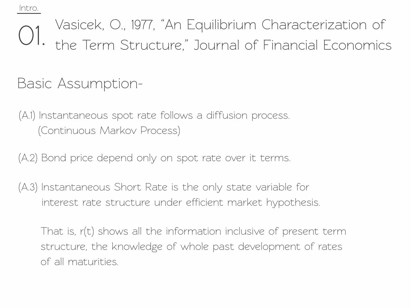
01. Vasicek, O., 1977, “An Equilibrium Charac'erization of

the Term Structure,” Journal of Financial Economics

Basic Assumption-

(A.3) Ins'an'aneous Short Ra'e is the only s'a'e variable for

in'erest ra'e structure under efficient market hypothesis.

That is, r(t) shows all the information inclusive of present 'erm

structure, the knowledge of whole past development of ra'es

of all maturities.

(A.1) Ins'an'aneous spot ra'e follows a diffusion process.

(Continuous Markov Process)

(A.2) Bond price depend only on spot ra'e over it 'erms.

Mean Reversion Property is not

a theorem, It is not a hypothesis, or

a conjecture as well. It’s a his'orical fact.

Intro.

01. Vasicek, O., 1977, “An Equilibrium Charac'erization of

the Term Structure,” Journal of Financial Economics

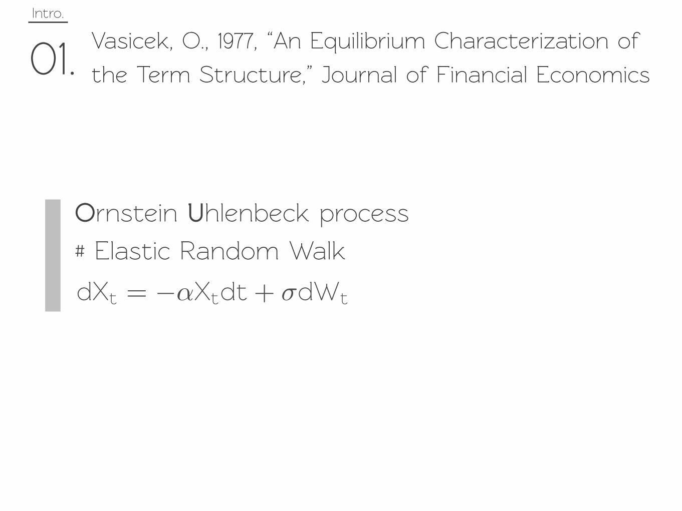
Orns'ein Uhlenbeck process

# Elastic Random Walk

dXt = ��Xtdt+ �dWt

Intro.

01. Vasicek, O., 1977, “An Equilibrium Charac'erization of

the Term Structure,” Journal of Financial Economics

Intro.

01. Vasicek, O., 1977, “An Equilibrium Charac'erization of

the Term Structure,” Journal of Financial Economics

Under risk-neutral probability measure (Q-measure),

drt = �(� � rt)dt+ �dWQtthe SDE of in'erest ra'e is :

Xt = rtektThen, we try 'o solve this differential equation. Let

By I'o’s Lemma, we could ob'ain: dXt = ektdrt + krtektdt

Thus, the solution of this SDE shows that:

rT = rte�k(T�t) + �(1 � e�k(T�t)) + �

� T

te�k(T�u)dWQ

u

Consider expec'ation under Q-measure:

EQ(rT) = rte�k(T�t) + �(1 � e�k(T�t))

T ∞ EQ(rT) = �

Intro.

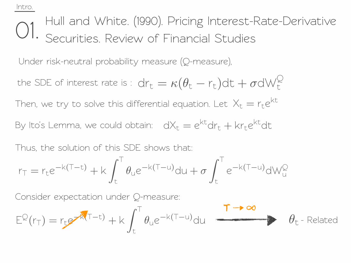
01. Hull and Whi'e. (1990). Pricing In'erest-Ra'e-Derivative

Securities. Review of Financial Studies

Under risk-neutral probability measure (Q-measure),

the SDE of in'erest ra'e is : drt = �(�t � rt)dt+ �dWQt

Xt = rtektThen, we try 'o solve this differential equation. Let

By I'o’s Lemma, we could ob'ain: dXt = ektdrt + krtektdt

Thus, the solution of this SDE shows that:

rT = rte�k(T�t) + k

� T

t�ue

�k(T�u)du+ �

� T

te�k(T�u)dWQ

u

Consider expec'ation under Q-measure:

EQ(rT) = rte�k(T�t) + k

� T

t�ue

�k(T�u)duT ∞

�t - Rela'ed

Let’s 'alk about the relation among

zero coupon bond price, ins'an'aneous

forward ra'e, and the'a function.

Intro.

01.

Intro.

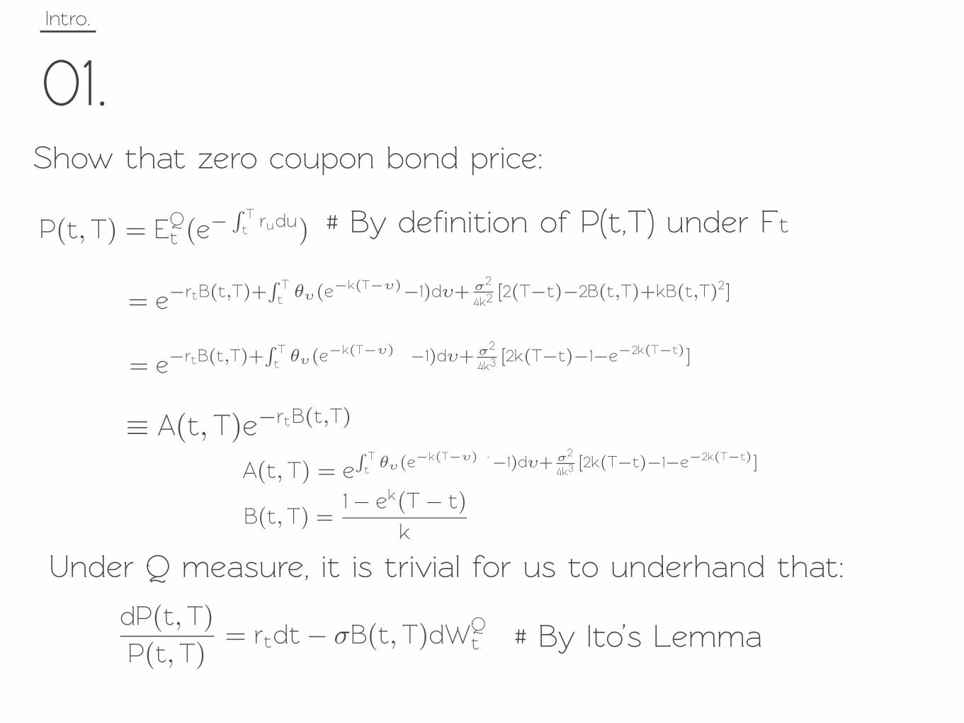
01.Show that zero coupon bond price:

= e�rtB(t,T)+� Tt ��(e�k(T��)��1)d�+ �2

4k3[2k(T�t)�1�e�2k(T�t)]

= e�rtB(t,T)+� Tt ��(e�k(T��)�1)d�+ �2

4k2[2(T�t)�2B(t,T)+kB(t,T)2]

� A(t,T)e�rtB(t,T)

B(t,T) =1 � ek(T � t)

k

A(t,T) = e� Tt ��(e�k(T��)��1)d�+ �2

4k3[2k(T�t)�1�e�2k(T�t)]

Under Q measure, it is trivial for us 'o underhand that:

dP(t,T)

P(t,T)= rtdt� �B(t,T)dWQ

t # By I'o’s Lemma

P(t,T) = EQt (e�� Tt rudu) # By definition of P(t,T) under Ft

Intro.

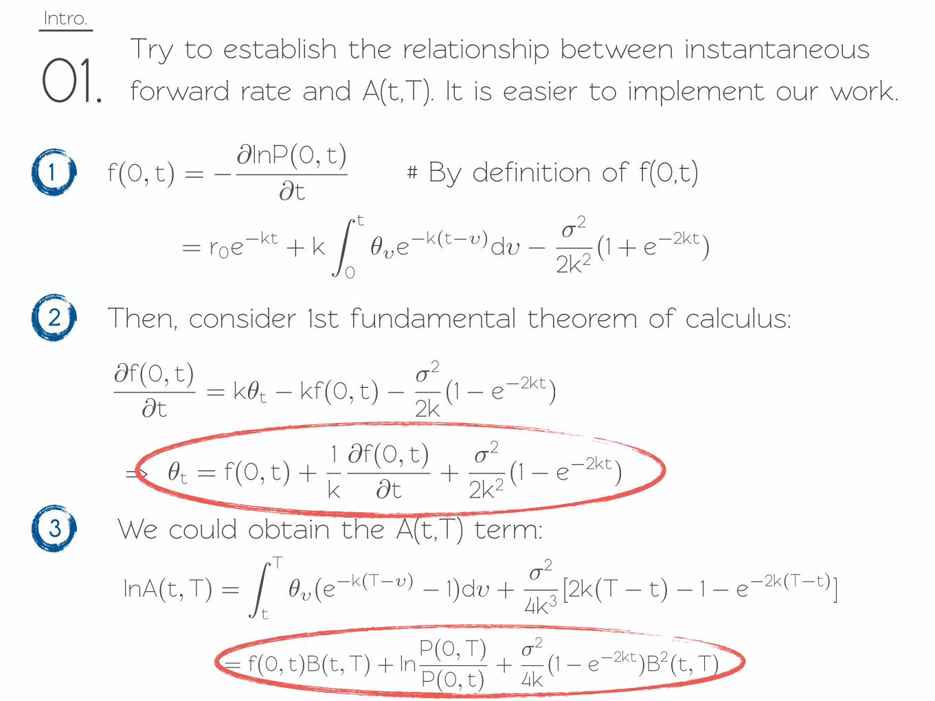
01.Try 'o es'ablish the relationship between ins'an'aneous

forward ra'e and A(t,T). It is easier 'o implement our work.

= f(0, t)B(t,T) + lnP(0,T)

P(0, t)+

�2

4k(1 � e�2kt)B2(t,T)

�t = f(0, t) +1k

�f(0, t)�t

+�2

2k2(1 � e�2kt)=>

f(0, t) = �� lnP(0, t)�t

= r0e�kt + k

� t

0��e

�k(t��)d� � �2

2k2(1 + e�2kt)

# By definition of f(0,t)1

�f(0, t)�t

= k�t � kf(0, t) � �2

2k(1 � e�2kt)

Then, consider 1st fundamen'al theorem of calculus: 2

lnA(t,T) =

� T

t��(e�k(T��) � 1)d� +

�2

4k3[2k(T � t) � 1 � e�2k(T�t)]

We could ob'ain the A(t,T) 'erm: 3

Furthermore, how 'o implement

the calibration work in our research ?

Intro.

01.

Empirical

02.

Empirical.

02. Da'a Description

1st da'a set is in'erest ra'e da'a in the period

of 1982/01/04 - 2013/12/31 from Fed Online. (7993 samples)

2nd da'a set is tradable T-bond price in US

at 2013/12/31 from Da'aStream. (221 samples)

3rd da'a set is yield ra'e curve at 2013/12/31 from

Fed Online.

We couldn’t use time series

method (o calibra(e parame(ers.

Empirical.

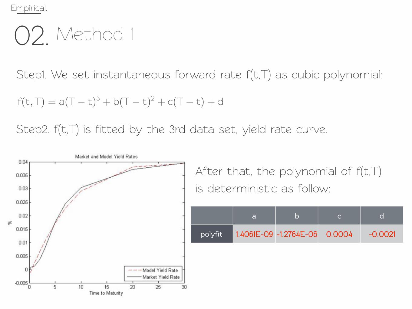
02.S'ep1. We set ins'an'aneous forward ra'e f(t,T) as cubic polynomial:

Method 1

f(t,T) = a(T � t)3 + b(T � t)2 + c(T � t) + d

S'ep2. f(t,T) is fit'ed by the 3rd da'a set, yield ra'e curve.

a b c d

polyfit 1.4061E-09 -1.2764E-06 0.0004 -0.0021

Af'er that, the polynomial of f(t,T)

is de'erministic as follow:

Empirical.

02.S'ep3. Cross Sectional Calibration

Method 1

B(0,T) = cT�

t=1

P(0, t) + FP(0,T)

A coupon bond is combination of several zero coupon bonds:

Given the market prices of Treasury bonds, the parame'ers

are calibra'ed by minimizing SSE.

� = arg m�in

n�i=1

(Bmarketi � Bmodel

i )2

n

k σ r0

Cross Sectional 3.616E-10 0.0306 0.033

Empirical.

02.S'ep4. Bonds price simulation is that :

Method 1

Yield Ra'e Curve can not capture the

behavior of ins'an'aneous forward.

Empirical.

02.

Empirical.

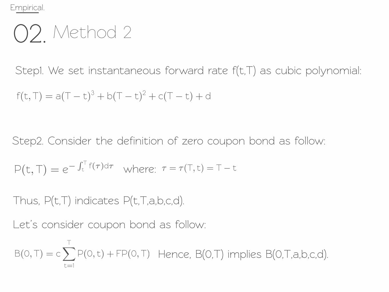
02.S'ep1. We set ins'an'aneous forward ra'e f(t,T) as cubic polynomial:

Method 2

f(t,T) = a(T � t)3 + b(T � t)2 + c(T � t) + d

S'ep2. Consider the definition of zero coupon bond as follow:

P(t,T) = e�� Tt f(�)d� � = �(T, t) = T � twhere:

Thus, P(t,T) indica'es P(t,T,a,b,c,d).

Let’s consider coupon bond as follow:

B(0,T) = cT�

t=1

P(0, t) + FP(0,T) Hence, B(0,T) implies B(0,T,a,b,c,d).

Empirical.

02.S'ep3. We could decide the coefficient of a, b, c, d by SSE condition:

Method 2

� = arg m�in

n�i=1

(Bmarketi � Bmodel

i )2

n

Af'er that, the polynomial of f(t,T) is de'erministic as follow:

# minimize the s'andard error of mean

a b c d

polyfit 1.6129E-05 -8.2566E-04 0.0125 -0.0057

�t = f(0, t) +1k

�f(0, t)�t

+�2

2k2(1 � e�2kt)

P(t,T) = A(t,T)e�rtB(t,T)

f(t,T) = a(T � t)3 + b(T � t)2 + c(T � t) + d

lnA(t,T) = f(0, t)B(t,T) + lnP(0,T)

P(0, t)+

�2

4k(1 � e�2kt)B2(t,T) B(t,T) =

1 � ek(T � t)k

P(t,T) = P(t,T,k,σ)

Empirical.

02. Method 2

S'ep4. Once again, coupon bond price shows that

B(0,T) = cT�

t=1

P(0, t) + FP(0,T) Hence, B(0,T) = B(t,T,k,σ)

Take the cross sectional calibration condition in'o our account:

� = arg m�in

n�i=1

(Bmarketi � Bmodel

i )2

n# minimize the s'andard error of mean

Af'er that, we ob'ain the parame'ers:

k σ r0

Cross Sectional 2.8414E-12 0.0112 0.2655

Empirical.

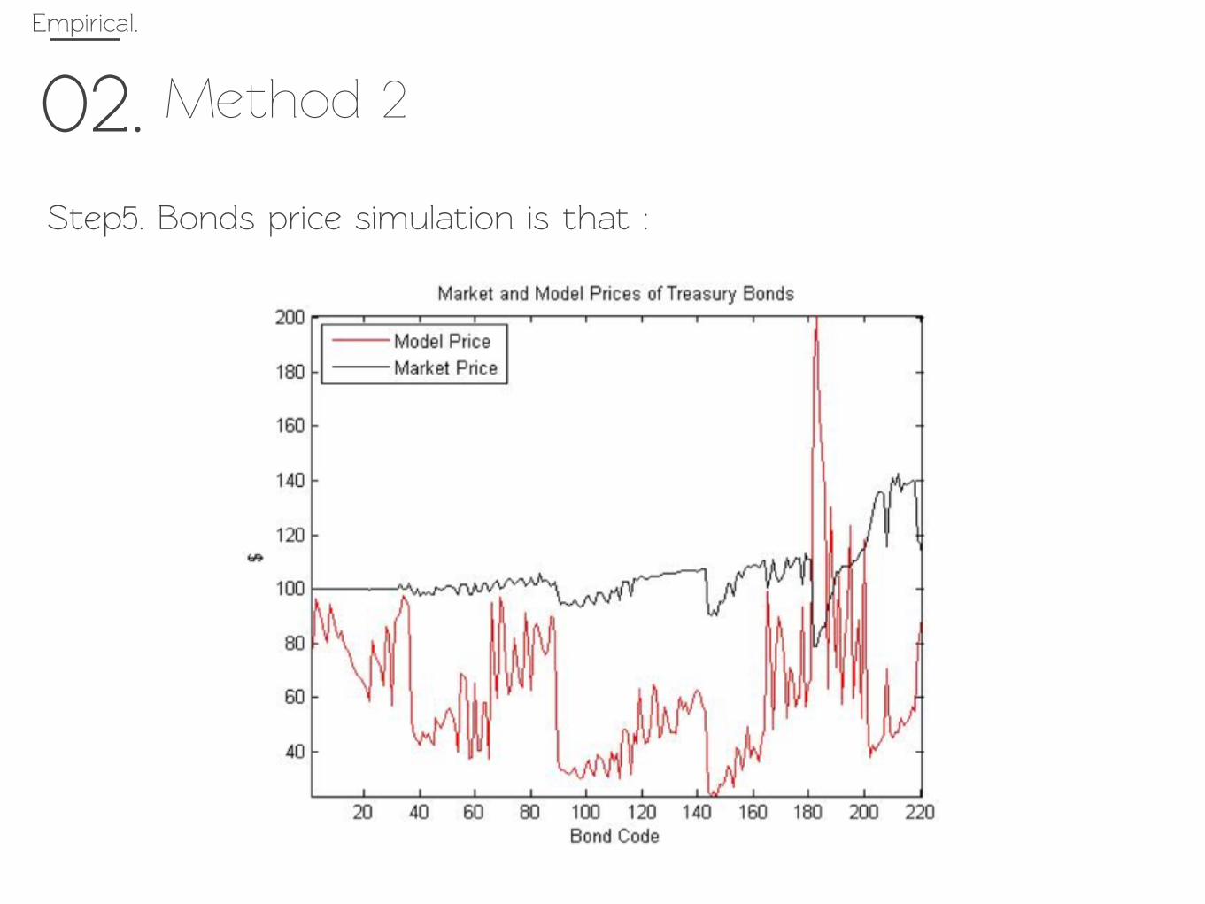
02. Method 2

S'ep5. Bonds price simulation is that :

Next, we 'end 'o calibra'e all the

parame'ers 'ogether one time.

Empirical.

02.

Empirical.

02. Method 3

S'ep1. We set ins'an'aneous forward ra'e f(t,T) as cubic polynomial:

f(t,T) = a(T � t)3 + b(T � t)2 + c(T � t) + d

S'ep2. Consider the definition of zero coupon bond as follow:

B(0,T) = cT�

t=1

P(0, t) + FP(0,T) B(0,T,a,b,c,d,k,σ)

�t = f(0, t) +1k

�f(0, t)�t

+�2

2k2(1 � e�2kt)

P(t,T) = A(t,T)e�rtB(t,T)

lnA(t,T) = f(0, t)B(t,T) + lnP(0,T)

P(0, t)+

�2

4k(1 � e�2kt)B2(t,T) B(t,T) =

1 � ek(T � t)k

where: P(0,T) = e�� T0 f(�)d� & P(0, t) = e�

� t0 f(�)d�

Therefore, under Hull Whi'e model

1

2

3

Empirical.

02. Method 3

S'ep3. Once again, consider cross sectional calibration condition:

� = arg m�in

n�i=1

(Bmarketi � Bmodel

i )2

n# minimize the s'andard error of mean

Af'er that, we ob'ain the parame'ers:

k σ r0 a b c d

Calibration 0.1905 0.0315 0.0012 1.3084E-06 6.5163E-05 -0.0033 -0.0035

Empirical.

02. Method 3

S'ep3. Bonds price simulation is that :

Eventually, method 3 is more sui'able for

calibrating these parame'ers in our work.

Empirical.

02.

Empirical.

02.Calcula'e the Yield Ra'e

P(t,T) = e�R(t,T)(T�t)k �,

We could get the model

zero-coupon bond price.

P(t,T) = A(t,T)e�rTB(t,T)

R(t,T) = � lnP(t,T)

T � t