Hugo Miguel Mota Magalhães - UMinho
45
Outubro de 2009 Universidade do Minho Escola de Engenharia Hugo Miguel Mota Magalhães Applying SAT on the Linear and Differential Cryptanalysis of the AES
Transcript of Hugo Miguel Mota Magalhães - UMinho

Outubro de 2009
Universidade do MinhoEscola de Engenharia
Hugo Miguel Mota Magalhães
Applying SAT on the Linear and DifferentialCryptanalysis of the AES
Tese de MestradoMestrado de Informática
Trabalho efectuado sob a orientação doProfessor Doutor Jose Manuel Valença
Outubro de 2009
Universidade do MinhoEscola de Engenharia
Hugo Miguel Mota Magalhães
Applying SAT on the Linear and DifferentialCryptanalysis of the AES


iii

ACKNOWLEDGMENTS
Firstly, I would like to thank my advisor, Professor Jose M. Valenca, to whom I
am deeply indebted, for his guidance throughout this last year. I would also like to
express my gratitude to my family, father, mother and brother for their uncoditional
support, my uncle, Manuel Magalhaes, for his words of advice, and to my cousin,
Pedro Magalhaes, for reviewing my thesis. Last but not least I would like to thank
my colleagues and friends Filipe Pina e Jose Rodrigues, for their companionship.
iv

ABSTRACT
The AES has been the encryption standard for the last few years, despite the
many attacks that have been attempted, none successfully broke the cipher. We will
explore some background concepts on cryptography and the importance of boolean
functions to the study of cryptanalysis. After, we will see what are SAT solvers, how
they operate and how they relate with cryptographic boolean functions, hence, their
importance on the cryptanalysis of ciphers. We follow with the description of AES
and how it was designed. In the last chapter we give an introduction to linear and
differential cryptanalysis, and why those attacks are infeasible against AES. Finally,
we will sum up what we have done, and provide future directions for research on what
is missing.
v

RESUMO
Nos ultimos anos a cifra AES tem sido a cifra padrao, apesar de ter sido alvo
de varios ataques, nenhum provou quebrar a cifra. Nos vamos explorar conceitos
criptgraficos e a importancia das funcoes booleanas no estudo da criptoanalise. De-
pois, vamos ver o que sao SAT solvers como eles operam e como eles se relacionam com
funcoes booleanas criptograficas, e dai, a sua importancia na criptoanalise das cifras.
Seguimos com a descricao do AES e como foi estruturado. Nos ultimo capıtulo damos
uma introducao a criptoanalise linear e diferencial, e o porque desses ataques nao
serem viaveis contra o AES. Finalmente, iremos resumir o que fizemos, e fornecemos
futuras direccoes para investigar o que ficou a faltar.
vi

TABLE OF CONTENTS
ABSTRACT . . . . . . . . . . . . . . . . . . . . . . . . . . . . . . . . . . . . . . . . . . . . . . . v
1 INTRODUCTION . . . . . . . . . . . . . . . . . . . . . . . . . . . . . . . . . . . . . . . 1
1.1 Objectives . . . . . . . . . . . . . . . . . . . . . . . . . . . . . . . . . . . . . . . . . . . . . . . . 2
2 BACKGROUND INFORMATION . . . . . . . . . . . . . . . . . . . . . . . . . . 3
2.1 Finite fields . . . . . . . . . . . . . . . . . . . . . . . . . . . . . . . . . . . . . . . . . . . . . . . 3
2.1.1 Groups, Rings, Fields . . . . . . . . . . . . . . . . . . . . . . . . . . . . . . . . . 3
2.1.2 Polynomials over Fields . . . . . . . . . . . . . . . . . . . . . . . . . . . . . . . . 5
2.2 Boolean Functions . . . . . . . . . . . . . . . . . . . . . . . . . . . . . . . . . . . . . . . . . 6
2.2.1 Definitions . . . . . . . . . . . . . . . . . . . . . . . . . . . . . . . . . . . . . . . . . . 6
2.2.2 Representation . . . . . . . . . . . . . . . . . . . . . . . . . . . . . . . . . . . . . . 7
2.2.3 Changing representation . . . . . . . . . . . . . . . . . . . . . . . . . . . . . . . 8
2.3 Ciphers . . . . . . . . . . . . . . . . . . . . . . . . . . . . . . . . . . . . . . . . . . . . . . . . . . 10
2.3.1 Introduction . . . . . . . . . . . . . . . . . . . . . . . . . . . . . . . . . . . . . . . . 11
2.3.2 Block cipher . . . . . . . . . . . . . . . . . . . . . . . . . . . . . . . . . . . . . . . . 12
2.3.3 Block cipher design . . . . . . . . . . . . . . . . . . . . . . . . . . . . . . . . . . . 13
3 BOOLEAN SATISFIABILITY PROBLEM . . . . . . . . . . . . . . . . . . . 16
3.1 Introduction . . . . . . . . . . . . . . . . . . . . . . . . . . . . . . . . . . . . . . . . . . . . . . 16
3.2 SAT Solvers . . . . . . . . . . . . . . . . . . . . . . . . . . . . . . . . . . . . . . . . . . . . . . 17
3.2.1 DPLL Algorithm . . . . . . . . . . . . . . . . . . . . . . . . . . . . . . . . . . . . . 17
3.3 Logical Cryptanalysis . . . . . . . . . . . . . . . . . . . . . . . . . . . . . . . . . . . . . . . 19
3.3.1 Encoding ciphers into CNF-SAT . . . . . . . . . . . . . . . . . . . . . . . . . 19
3.3.2 Application of SAT solvers . . . . . . . . . . . . . . . . . . . . . . . . . . . . . 20
4 ADVANCED ENCRYPTION STANDARD . . . . . . . . . . . . . . . . . . . 21
4.1 Specification . . . . . . . . . . . . . . . . . . . . . . . . . . . . . . . . . . . . . . . . . . . . . . 21
4.2 Strucutre . . . . . . . . . . . . . . . . . . . . . . . . . . . . . . . . . . . . . . . . . . . . . . . . 21
vii

4.2.1 The round transformations . . . . . . . . . . . . . . . . . . . . . . . . . . . . . 22
4.2.2 The Key Schedule . . . . . . . . . . . . . . . . . . . . . . . . . . . . . . . . . . . . 25
4.3 High-level implementation . . . . . . . . . . . . . . . . . . . . . . . . . . . . . . . . . . . 25
5 CRYPTANALYSIS . . . . . . . . . . . . . . . . . . . . . . . . . . . . . . . . . . . . . . . 27
5.1 Linear Cryptanalysis . . . . . . . . . . . . . . . . . . . . . . . . . . . . . . . . . . . . . . . 27
5.2 Differential Cryptanalysis . . . . . . . . . . . . . . . . . . . . . . . . . . . . . . . . . . . . 30
6 CONCLUSIONS . . . . . . . . . . . . . . . . . . . . . . . . . . . . . . . . . . . . . . . . . 32
6.1 What have we done so far? . . . . . . . . . . . . . . . . . . . . . . . . . . . . . . . . . . . 32
6.2 Future directions . . . . . . . . . . . . . . . . . . . . . . . . . . . . . . . . . . . . . . . . . . 32
REFERENCES . . . . . . . . . . . . . . . . . . . . . . . . . . . . . . . . . . . . . . . . . . . . . 33
viii

1
CHAPTER 1
INTRODUCTION
With the evolution and popularity of the Internet, security and privacy issues became
a recurring theme for researchers. From this research the first modern cryptographic
algorithms started to appear. This algorithms, also known as ciphers, were used
to encrypt sensitive data sent over the insecure global system of interconnected
networks. The science of securely transmitting information is known as cryptology.
The science that studies and analyzes ciphers is called cryptography and, itself, is a
field of cryptology.
The term encryption refers to the act of taking unobfuscated information, the
plaintext, and applying the cipher to obtain obfuscated data, the ciphertext. To the
inverse action, from the ciphertext derive the plaintext, we call decryption. Generally,
an external piece of information, called the key, is used in the encryption process.
The standard encryption cipher from 1975 until 2002 was the Data Encryption
Standard (DES) [14]. As is common with every other cipher, DES was thoroughly
analyzed and eventually major flaws were found [4, 31]. This flaws compromised
the cipher in such manner that data encrypted with DES was not considered secure
anymore, this led to the necessity of finding a new encryption standard. In 1997 the
US National Institute of Standards and Technology (NIST) announced a competition
for new cryptographic algorithms. From the competition emerged a cipher named
Rijndael, which later became known as the Advanced Encryption Standard (AES) [1,
10] and was adopted by the U.S. government. The AES was also adopted rapidly by a
wide majority of important organizations such as banks, humanitarian and military.
Being a standard, and as happened before with DES and every other cipher, it is
of crucial importance to study ways to circumvent AES protection and to study its
weaknesses. Until the time of writing no feasible method was found to break AES.
The study of methods to analyze and defeat cryptographic algorithms is called crypt-
analysis. Among the various methods of cryptanalysis, in this thesis, we are going to

2
focus on Linear Cryptanalysis [32] and Differential Cryptanalysis [3]. The purpose of
Linear Cryptanalysis is to obtain a linear approximate expression to the actions of a
cipher, this way we can apply these equations with known plaintext/ciphertext pairs
to derive bits from the encryption key. On the other hand, Differential Cryptanalysis
consists on analyzing the effect of a cipher on pairs of plaintext and the resulting
output in order to find statistical patterns. If patterns are found we can conclude,
thus, that the cipher is not random.
Both analyzes heavily rely on the properties of boolean functions. This functions
are the core in which the security of most ciphers rely, thus, the study of boolean
functions have been growing for the past few years, leading to new discoveries and
innovations on the field. One of those innovations is the application of spectral
functions in mathematics.
From the analyzes of function spectra it is possible to to reduce complex problems
of cryptanalysis into boolean problems known as Boolean Satisfiability (SAT) prob-
lems. SAT relies on the boolean characteristic of a problem and attemps to find a truth
solution to that problem. In the last decade a remarkable number of SAT solvers were
published [16, 20, 37]. The performance of state-of-the-art solvers made it possible to
apply them to fields never thought before, such as cryptanalysis [13, 28, 29, 35].
1.1 Objectives
The main purpose of this thesis, is to study the feasibility of attacking a cipher using
SAT and to analyze the current cryptanalysis state of AES, the most popular cipher
used today.
Firstly, we must overview how to represent data using finite fields, since most
attacks rely on the representation of bits as finite fields. We will then give an insight
of boolean functions, and though they are not going to be directly applied into this
thesis, their understading is crucial for the design of ciphers and therefore how to
attack them. Provided that we are dealing with ciphers, a review on the matter will
also be given. Only after this fundamental concepts are explained, will we describe
SAT and how to apply it to the field of cryptography. Moreover, before delving into
cryptanalysis, a chapter will be dedicated to AES cipher. Finally, we round up with
what have we done and provide future directions that may be taken after this work.

3
CHAPTER 2
BACKGROUND INFORMATION
Before proceeding we will give some important mathematical background, that will
be used throughout this thesis, as well as, a brief introduction to the cryptographic
concept of ciphers. This chapter is organized as follows. Section 2.1 provides theory
on finite fields. The second section, section 2.2, covers boolean functions. Finally,
section 2.3 overviews cryptographic concepts.
2.1 Finite fields
In this section we present an introduction to the theory of finite fields, for further
reference we recommend the reading of [25, 33].
2.1.1 Groups, Rings, Fields
In order to explain finite fields we must start with the foundations, and so, we will
begin discussing Abelian groups.
An Abelian group < G,+ > is a set G of elements with a group operation, denoted
here by ′+′. The elements of the Abelian group are said to be ”under” the group
operation.
The group operation has the following properties:
1. Closure: ∀a, b ∈ G : a+ b ∈ G
2. Associativity: ∀a, b, c ∈ G : (a+ b) + c = a+ (b+ c)
3. Neutral element: ∃0 ∈ G,∀a ∈ G : a+ 0 = a
4. Inverse: ∀a ∈ G,∃b ∈ G : a+ b = 0

4
5. Commutativity: ∀a, b ∈ G : a+ b = b+ a
We can now define a ring < R,+, · > as a set R of elements with two group
operations which fulfill the following conditions:
1. < R,+, · > is an Abelian group.
2. Multiplicative closure.
3. Multiplicative associativity.
4. Multiplicative identity: ∃1 ∈ R, ∀a ∈ G : a · 1 = a
5. Left and right distribution: ∀a, b, c ∈ R : (a+ b) · c = a · (b+ c)
A ring is said to be commutative ring if the multiplication is commutative.
A structure < F,+, · > is said to be a field if:
1. < F,+, · > is a commutative ring.
2. Multiplicative inverse, except in 0: ∀a 6= 0 ∈ F∃a−1 ∈ F : ∀a 6= 0, a · a−1 = 1
Finally, we define a finite field, or Galois field, as a field with finite number of
elements. To the number of elements in the set we call order. The order of every
finite field is a prime p or a power of a prime pn, with n being any positive integer.
To p we call the characteristic of the finite field, i.e., the p-fold sum of the identity 1
with itself is 0.
For each prime power, pn, there exists exactly one finite field, denoted by GF (pn).
In other words, fields of the same order are isomorphic. The elements of GF (p) can
be represented by the integers 0, 1, .., p− 1.
The two operations of a finite field, addition and multiplication, are modulo p. If
n > 1, the operations under GF (pn) are modulo an irreducible polynomial of degree
n. The elements of GF (pn), 0, x0, x1, ..., can be represented as polynomials with
degree less than n.

5
2.1.2 Polynomials over Fields
A polynomial over a field F is expressed as:
f(x) =n∑i=0
aixi = a0 + a1x+ ...+ an−1x
n−1,
where n is a positive integer and the coefficients ai ∈ F . The set of polynomials over
a field F is denoted by F [x]. The degree of a polynomial is the greatest n, such that,
an 6= 0. The set of polynomials over a field F , which have a degree less than n, is
denoted by F [x]|n.
Polynomials of degree n over a field F can be stored as strings of bits, which in
turn can be abbreviated using the hexadecimal notation.
Example 2.1.2.1 The polynomial in GF (2)|8, x7 + x4 + x3 + x + 1 corresponds to
10011011 in binary and 9B in hexadeciaml.
We can, in this way, consider a byte as a polynomial with coefficients in GF (2):
b7b6b5b4b3b2b1b0 7→ b(x)
b(x) = b7x7 + b6x
6 + b5x5 + b4x
4 + b3x3 + b2x
2 + b1x+ b0.
The set of all possible byte values corresponds to the set of all polynomials with
degree less than eight.
Operations on polynomials is defined as follows:
Addition: c(x) = a(x) + b(x)↔ ci ≡ ai + bi (mod p), 0 ≤ i < n,
where p is the characteristic of the finite field. If the finite field as characteristic 2
the addition can be implemented using the XOR operation, ⊕ .
Example 2.1.2.2 Let F be the field GF (2). The sum of the polynomials 53 + CA
is 99:
(x6 + x4 + x+ 1)⊕ (x7 + x6 + x3 + x) = x7 + (1⊕ 1)x6 + x4 + x3 + (1⊕ 1)x+ 1
= x7 + x4 + x3 + 1
In binary: 01010011⊕ 11001010 = 10011001

6
Multiplication: c(x) = a(x) · b(x)↔ c(x) ≡ a(x)× b(x) (modm(x)),
where m(x) is an irreducible polynomial over the field GF (p).
Example 2.1.2.3 Let us consider the field GF (28) and the irreducible polynomial
m(x) = x8 +x4 +x3 +x+ 1, which happens to be the AES irreducible polynomial, the
product of the polynomials 53× CA is 01:
(x6 + x4 + x+ 1)× (x7 + x6 + x3 + x) = (x13 + x11 + x8 + x7)⊕ (x12 + x10 + x7 + x6)
⊕ (x9 + x7 + x4 + x3)⊕ (x7 + x5 + x2 + x)
= x13 + x12 + x11 + x10 + x9 + x8 + x6
+ x5 + x4 + x3 + x2 + x
and
(x13 + x12 + x11 + x10 + x9 + x8+x6 + x5 + x4 + x3 + x2 + x)
≡ 1 (mod x8 + x4 + x3 + x+ 1)
2.2 Boolean Functions
Boolean Functions play an important role in the design of ciphers, given that they are
the target of linear and differential cryptanalysis. In order to design strong ciphers,
boolean functions must be carefully chosen and thorough tests must be perfomed. In
this section we aim to provide tools to manipulate boolean functions.
Boolean functions are defined as functions that take as input a finite bitstring and
output a bitstring of the same size or a single bit. More formally we can define a
boolean function as: f : Bn → Bn or f : Bn → B.
We will focus on boolean functions with multiple variables: f : GF (2)n → GF (2)
and then we will see how to change the represention from GF (2)n to GF (2n).
2.2.1 Definitions
The Hamming weight of a vector x = (x0, x1, ...xn−1), xi ∈ {0, 1}, denoted by wt(x),
is the number of non-zero positions of that vector. The support of x contains the
non-zero positions of that vector and is denoted by sup(x), i.e., sup(x) = {i : xi 6= 0}.
7
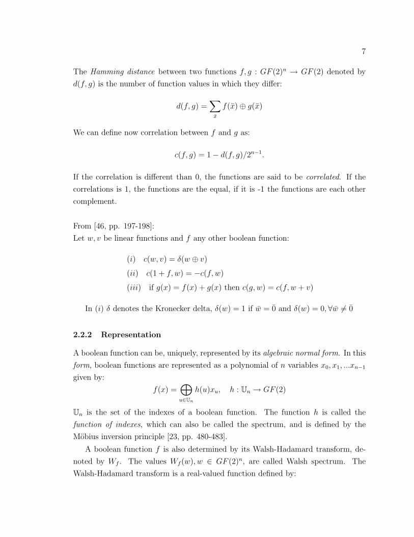
The Hamming distance between two functions f, g : GF (2)n → GF (2) denoted by
d(f, g) is the number of function values in which they differ:
d(f, g) =∑x
f(x)⊕ g(x)
We can define now correlation between f and g as:
c(f, g) = 1− d(f, g)/2n−1.
If the correlation is different than 0, the functions are said to be correlated. If the
correlations is 1, the functions are the equal, if it is -1 the functions are each other
complement.
From [46, pp. 197-198]:
Let w, v be linear functions and f any other boolean function:
(i) c(w, v) = δ(w ⊕ v)
(ii) c(1 + f, w) = −c(f, w)
(iii) if g(x) = f(x) + g(x) then c(g, w) = c(f, w + v)
In (i) δ denotes the Kronecker delta, δ(w) = 1 if w = 0 and δ(w) = 0,∀w 6= 0
2.2.2 Representation
A boolean function can be, uniquely, represented by its algebraic normal form. In this
form, boolean functions are represented as a polynomial of n variables x0, x1, ...xn−1
given by:
f(x) =⊕u∈Un
h(u)xu, h : Un → GF (2)
Un is the set of the indexes of a boolean function. The function h is called the
function of indexes, which can also be called the spectrum, and is defined by the
Mobius inversion principle [23, pp. 480-483].
A boolean function f is also determined by its Walsh-Hadamard transform, de-
noted by Wf . The values Wf (w), w ∈ GF (2)n, are called Walsh spectrum. The
Walsh-Hadamard transform is a real-valued function defined by:

8
Wf (w) =∑
x∈GF (2)n
(−1)f(x)⊕x·w = 2n − 2wt(f ⊕ x · w)
The function (−1)f can be constructed by the inverse Walsh-Hadamard:
(−1)f(x) = 2−n∑
w∈GF (2)n
Wf (w)(−1)w·x
From the Walsh spectrum we can define the following properties [44]:
1. Balanced - A boolean function f is said to be balanced if its output is equally
distributed, wt(f) = 2n−1. In terms of Walsh spectrum we get Wf (0) = 0;
2. Nonlinearity - The nonlinearity of a boolean function f is defined by the min-
imum distance of the function to the set of affine functions, A, and is den-
toted by Nf = ming∈Ad(f, g), or in terms of the Walsh transform as Nf =
2n−1 − 12maxw∈GF (2)n|Wf (w)|.
3. Correlation immunity - A boolean function f is said to be correlation immune
of order t if Wf (w) = 0, for 1 ≤ wt(w) ≤ t. That is if the output and any t of
its inputs are statistically independent;
It is trivial to notice the importance of the above properties and the impact that they
have on the the design of ciphers. The balanceness of a function gives the amount
entropy, or uncertainty over the value of f . High nonlinearity prevents the actions of
the cipher being approximated by affine functions, thus, reducing the risk of the cipher
being vulnerable to correlation, linear, and other attacks. If the cipher has highly
immunity to correlation, it helps preventing differential and correlation attacks. We
have just demonstrated the importance of studying the Walsh transform of boolean
functions.
2.2.3 Changing representation
In this section we will demonstrate how to change the representation from GF (2)n to
GF (2n) [46, §3.4]. A function f : GF (2n)→ GF (2n) can be interpreted as an S-Box
n× n, which will be covered later, and is represented by:
f(x) =2n−1∑i=0
aixi, ai ∈ GF (2n).

9
Some tools are provided below in order to aid in the process of changing the
representation of boolean functions.
We start by defining the function (·)σ : GF (2n) → GF (2n)n which turns an
element x of the Galois field into the vector, over that field, formed by all σk(x):
xσ = (x, σ(x), σ2(x), ..., σn−1(x))
σ(x) is the Frobenius endomorphism σ : x → x2. Now it is possible to represent
linear transformations using matrix algebra. With this in mind we can express a
linear function f as:
f(x) =n−1∑k=0
akσk(x), ak ∈ K
K is any extension ofGF (2) and a ∈ GF (2). If we denote a by the vector (a0, a1, ..., an)
we can represent the above polynomial by the dot product of two vectors:
f(x) = axσ
The above indicates that for a given function y = f(x) = a · xσ we can express yσ as:
yσ = Axσ,
where A denotes the matrix: Aij = (ak)2i, k = j − 1(mod n− 1).
Let B be a base of GF (2n). A base determines n projections, i.e., boolean functions
pu : GF (2n)→ GF (2), one for each element u ∈ B, in such way that any x ∈ GF (2n)
may be reconstructed by using the elements u and the values of pu(x):
x =∑u∈B
pu(x)u
We denote the function that maps x to its projections vector by (·)∼ : GF (2n) →GF (2)n. The above equation can now be defined vectorially as:
x = B · x∼
For any element u ∈ B of a base of GF (2n) exists one, and only one, element
u′ ∈ GF (2n), called dual element of u, such as, for all x ∈ GF (2n) we have:

10
pu(x) = tr(u′x) = (u′)σ · xσ
where tr represents the trace function. The set B′ = u′|u ∈ B of all the dual elements
creates a new base of GF (2n) that will be called dual base of B. It is possible to
prove that B and B′ are relacted by B′ = T−1B, T is the trace matrix Tuv = tr(uv).
This notion of dual element can be extended to any x ∈ GF (2n). The dual element
of x in base B, denoted by x′, is in GF (2n) and has exactly the same components of
x but in B′:pu(x) = tr(u′x) = tr(ux)′ = pu′(x
′), ∀u ∈ B
The operation (·)∼ maps every element of a base B of GF (2n) to the vector of its
projections on that base. Thus
x′∼ = T−1x∼, x′ = B · x′∼ = B′ · x∼
The operator (·)σ can be extended to vectors of elements GF (2n). Let A ∈ GF (2n)n,
then the matrix Aσ ∈ GF (2n)n×n has, for line of order i, the vector (Ai)σ, i.e.,
(Aσ)ik = σk(Ai). Under this circumstances, if B,B′ are a pair of dual bases then:
1. (B′)σ = T−1Bσ
2. x∼ = (B′)σxσ and xσ = (Bσ)tx∼
3. (Bσ)tBσ = T and (Bσ)t(B′)σ = I
4. Bσ(x′)σ = (B′)σxσ
All the above notions are important when we want to study boolean functions that
require changing representation. This happens when a function, alternately, uses bits
in GF (2n) and GF (2)n. We can now solve the following problem:
”Given a base B in GF (2n) and a function f∼ of domain GF (2)n, construct a
function f of domain GF (2n) that verifies f∼(x∼) = f(x)∼, ∀x. Or given a function
f , construct f∼”.
2.3 Ciphers
There are some important concepts in cryptology we must define. For an excellent
treatment on the subject we refer to the the book of Menezes et al. [34].

11
2.3.1 Introduction
A cryptosystem is a five-tuple (P , C, K, E , D), where:
1. P is the plaintext;
2. C is the ciphertext;
3. K is the key;
4. EK is the encryption function under the key K;
5. DK is the decryption function under the key K.
and the following property holds, DK(EK(x)) = x,∀x ∈ P . Reiterating the
definition of a cipher, which is an algorithm that obfuscates data, it becomes obvious
that EK is a cipher.
In his classic paper [41], Shannon, proposed several criteria for the design of
ciphers:
1. The amount of secrecy required should dictate how much effort we put into
securing, or encrypting, our data.
2. The cryptographic system should be low in complexity and simple to implement.
3. The size of the ciphertext should be less than or equal to the size of the plaintext.
4. Errors should not propagate.
There are two types of cryptographic schemes which involve a key: the public-
key cryptosystem and the symmetric-key cryptosystem (also known as private-key
ciphers). The main difference between them is the secrecy of the key. Whereas in
public-key cryptosystems there are two keys, a public and a private, in symmetric-key
cryptosystems the same key is shared by both parties.
Private-key schemes can be further divided into block ciphers or stream ciphers.
Stream ciphers, typically operate at bit level using linear feedback shift registers
(LFSR). Perhaps the most widely used stream ciphers are RC4 [43], used in wired
equivalent privacy (WEP) and secure sockets layer (SSL). The other being A5 [49],
used in mobile telecommunications. Every stream cipher tries to approach its design

12
to the design of one-time pad (OTP), the only cipher ever being proved perfectly
secure [41]. Due to the key size required by the OTP (which must be the same size
as the plaintext), the cipher is impractical.
On the other hand, block ciphers (e.g. AES [1, 10], DES [14]) operate on groups
of bits. Being the object of study of this thesis we shall delve into block ciphers.
2.3.2 Block cipher
To restate, block ciphers take as input a cipher key and groups of plaintext text
bits, called blocks, of fixed length, and output ciphertext blocks of the same length.
Precisely, a block cipher is a set of boolean transformations operating on n-bit vectors.
Most block ciphers are iterative block ciphers. In an iterative block cipher the
plaintext block is encrypted in rounds. In each round a set of boolean transformations,
called round functions, are applied to an intermediate result, the state, using the round
key. The round key is a subkey derived from the cipher key in a process called key
schedule. As the name suggests, the round key is unique for each round. To the
concatenation of all round keys we call the expanded key. The security level of an
iterative block cipher is achieved by increasing the number of rounds.
If an iterative block cipher uses the same round transformations in all rounds,
except in the first or last round, the cipher is called an iterated block cipher.
Figure 2.1: Iterative block cipher with three rounds. [10, p. 25]

13
Another class of block ciphers are the key-alternating block ciphers, which are
iterative block ciphers with the following properties:
1. Alternation: The cipher is defined as the alternated application of key-independent
round transformations and key additions. The first round key is added before
the first round and the last key is added after the last round.
2. Simple key addition: The round keys are added to the state by means of a
simple XOR.
Key-alternating block ciphers, too, have a special case the key-iterated block ci-
phers, which are a junction of iterated block ciphers with key-alternating block
ciphers.
Figure 2.2: Key-alternating block cipher with two rounds. [10, p. 26]
2.3.3 Block cipher design
The design of block ciphers, concentrates around the concepts of confusion and
diffusion, coined by Shannon [41]. Confusion focus on the relation between the
ciphertext and the key, attempting to mix their bits. In practice, confusion is achieved
through the use of substitution boxes (S-box). Diffusion acts on an entire block

14
performing series of linear transformations, spreading its bits, in order to prevent
redundancy. This is achieved by the use of permutation boxes (P-box).
A S-box can be defined as a lookup table with 2n words of m bits each, thus,
S-boxes are usually referred as nxm S-boxes, i.e., an S-box that takes as input n bits
and returns m bits. A S-box that takes as input many bits as the output is called
squared. Formally, a S-box, S, is defined as:
S : GF (2)n 7→ GF (2)m
An S-box must be carefully chosen to satisfy various cryptographic properties [36, 48],
such as: highly nonlinearity, correlation immunity, high avalance features, etc.
A P-box, in a similar way as a S-box, is defined as a lookup table, but contrarily
to the S-boxes, P-boxes do not change the input instead they map the input to a
different output value. Given this fact we can conclude, thus, that P-boxes are not
as random as S-boxes, since we can establish a one-to-one correspondence of bits.
Looking back, at the two previously mentioned structures, it is trivial to notice
that neither should be used alone. A previous knowledge of the S-box or P-box would
make it trivial to decrypt a message. To advert this situtation other structures have
been created that involve the use of the previous ones.
An obvious extension is to combine both structures, and that is what a substitution-
permutation network (SPN) is. Normally, there is a layer of one or more S-boxes,
providing confusion, followed by another layer of one or more P-boxes, contributing
to diffusion, or vice-versa. However, it still is relatively easy to relate the input to
the output, therefore, the use of a key-schedule is useful. As mentioned before, the
key-schedule derives from the key a subkey, that will be added to the cipher, usually,
by XORing them together with either the bits from the S-box or P-box. This makes
it possible for SPNs to be used by theirselves or integrated in a Feistel structure. One
point to note, is the fact that SPNs need two different algorithms, one for encryption
and another for decryption. A notable cipher that uses a SPN by itself is AES.
A Feistel structure, uses a technique to avoid the use of two different algorithms
(one to encrypt, the other to decrypt). This technique consists of splitting a block
in two parts, Li−1 and Ri−1. The round function,f , takes as input a half-sized block
and a round key, Ki. In each round, the left part, Li, will be formed by Ri−1 and the
right part, Ri, will result from the XOR of Li−1 with the Ki. Formally we have:

15
Li = Ri−1
Ri = Li−1 ⊕ f(Ri−1, Ki).
The decryption function, regardless if the round function is nonlinear or noninvertible,
is processed as:
Ri−1 = Li
Li−1 = Ri ⊕ f(Li, Ki)
There are some ciphers that use Feistel structures in which the blocks are not divided
in equal halves, those are called unbalanced Feistel ciphers. The Skipjack, is an
example of such cipher. The ciphers DES, Blowfish, RC5, to name a few, are among
the ciphers that use a Feistel structure.
Figure 2.3: A substitution-permutationnetwork. Figure 2.4: A feistel structure.

16
CHAPTER 3
BOOLEAN SATISFIABILITY PROBLEM
In this chapter we will overview what is the Boolean Satisfiability Problem (SAT).
We will then take a look at which satisfiability algorithms, known as SAT solvers,
have been developed such as in what class do they belong. We end up this chapter
with theory on how to apply SAT solvers against ciphers.
3.1 Introduction
SAT solvers try to answer the question: ”Given a propositional formula, does it have
a solution ?”. In practical terms, not only is the decision problem of interest but also
the actual assignment that makes the decision true, if any. If exists any assignment
of variables in the formula which make the decision true, then the formula is said to
be satisfiable, otherwise, it is said to be unsatisfiable.
Propositional or Boolean formulas are, generally, represented in the conjuctive
normal form (CNF), which is represented by a conjuction of clauses. Clauses, in
turn, are built from literals. These literals are, nothing more, than a variable x which
take a value in the set {0, 1} and are known as negative literal or positive literal,
respectively. The complement of a variable x is denoted by ¬x. So in CNF we have,
the clauses c which are disjunction of literals l, c = (l1 ∨ l2 ∨ ...∨ ln), and are denoted
by: c = {l1, l2, ..., ln}. A function f is in the CNF if it represents a disjunction of
clauses, i.e., f = (c1 ∧ c2 ∧ ...∧ cn). As with the clauses a function can be denoted as
f = {c1, c2, ..., cn}. A function in CNF can also be expressed as:
f = {{l1,1, ..., l1,i1}, {l2,1, ..., l2,i2}, ..., {ln,1, ..., ln,in}}
A CNF f is satisfied iff all clauses are satisfied. A clause c is satisfied iff at least
a literal in c is satisfied. In turn, a literal l is satisfied iff (l = xi, and xi = 1) or

17
(l = ¬xi, and xi = 0).
By analogy, a CNF f is unsatisfied if any clause is not satisfied. A clause c is said
to be unsatisfied iff all literals in c are unsatisfied 1. Finally, a literal l is unsatisfied
iff (l = xi, and xi = 0) or (l = ¬xi, and xi = 1).
3.2 SAT Solvers
There are many methods of solving SAT problems. Each method can be divided into
two groups, the systematic methods and the local search methods.
Systematic methods, also known as complete methods, given a formula either
produce an assignment that satisfies the formula or prove that the formula is unsat-
isfiable. The best complete solvers are based on a process introduced several years
ago, the Davis-Putnam procedure. Since the introduction of the procedure many
improvements have been proposed, the most notorious being the Davis, Putnam,
Logemann and Loveland (DPLL) modification. DPLL algorithms are based on ex-
haustive branching and backtracking search. Some systematic SAT solvers based on
the DPLL procedure are: SATO [50], zChaff [37], MiniSat [16] and more recently
BerkMin [20].
On the other hand, local search methods, or incomplete methods, are not guaran-
teed to find any satisfying assignment neither prove the given formula is unsatisfiable.
Incomplete methods are based on heuristics, the reason, they do not provide any
guarantees on the satisfiability of a formula. The most influencial incomplete methods
are GSAT [40] and WalkSAT [39]. GSAT is based on a randomized local search
technique, whereas, WalkSAT introduces some noise into that same randomization
technique.
3.2.1 DPLL Algorithm
In 1962, Davis, Logemann and Loveland proposed a modification [12] of the original
Davis&Putnam algorithm [11]. Behind the motivation for this modification was the
fact that the original algorithm required exponential space for resolving Boolean
formulas. In DPLL, the authors introduced a branching rule while resolving formulas
in order to tradeoff space for time.
1A clause that contains no literals is called empty and is always unsatisfied

18
With optimization in mind, modern SAT solvers started to introduce some new
features to the DPLL procedure.
Branching rules, are the key strategy to the efficiency of a solver, a survey com-
paring the various branching rules, or decision strategies, is available [26]. Newer
variations on branching rules were used in BerkMin [20] and MiniSat [17].
Clause learning, helped to improve, in great manner, the success of state-of-the-art
SAT solvers. The basic idea is to cache causes of conflicts and use this information to
cut off similar conflicts encountered later during the search. It is used in the majority
of modern solvers.
Conflict clause minimization was introduced in MiniSat [17], the main purpose is
to reduce the size of learnt conflict clause by removing any literals, on that clause,
that are implied to be false when the rest of the literals are set to false.
Conflict-directed backjumping [38] is used to skip decision levels by using learnt
clauses to skip the last assignment in a clause. It is used in relsat [2] and GRASP [27].
Randomized restarts are used by setting a treshold value to some parameter, when
that limit is reached the search starts from the beginning but the all the learnt clauses
are treated as additional initial clauses. This method was introduced in the paper [21].
Watched literals scheme, maintain a ’watch’ on two literals for each clause not yet
satisfied and that are not false under the current assignment. These literals could be
set to true or keep unassigned. The clause can then be checked for satisfiability by
checking weather at least one of the ’watched’ literals is true. This scheme was first
introduced in zChaff [37].
The DPLL algoritm proposed in 1962 works as follows. It chooses a literal and
assigns the truth value to it, then, simplifies the formula and recursively checks if
the formula is satisfiable. If a clause contains only one unassigned literal, this clause
can only be satisfied by assigning the value that makes the clause true, this is called
unit propagation and prevents unnecessary recursion, narrowing the search space. To
further narrow the search space pure literal elimination is also used, i.e., if a variable
exists always with the same boolean value it can be assigned in such way that all
clauses containing it are true, therefore those clauses can be eliminated. Given the
case that the formula is not satisfied, the same run is done but assigning the false value
to the literal. While simplifying, the clauses which become true with the assignment
19
are eliminated and so are all the literals that become false.
Example 3.2.1.1 Let us try a = true, and with the formula f :
f = (a ∨ b) ∧ (¬a ∨ c) ∧ (¬b ∨ c)
then we simplify by removing the clauses which became true
f = (¬a ∨ c) ∧ (¬b ∨ c)
we now simplify by eliminating ¬a
f = (c) ∧ (¬b ∨ c)
after this point is clear that c must be true and thus the formula is satisfiable.
3.3 Logical Cryptanalysis
As we have stated before, the heart of many cryptographic techniques lies in the
strength of boolean functions. With the advance of SAT solvers, primarily due to
the field of Artificial Intelligence, the next logic step was to apply the solvers on
cryptographic boolean functions, and thus, Logical Cryptanalysis was born [30].
3.3.1 Encoding ciphers into CNF-SAT
In order for logical cryptanalysis to be of any use when applied to ciphers, some
pre-processing must be effected, more precisely the cipher must be encoded into a SAT
problem, i.e., the cipher must be converted to the CNF. To achieve that conversion a
few methods have been purposed in literature. In the original paper [30], the authors
tried to directly convert each cipher operation by walking throught the cipher and
represent each operation as a circuit. This kind of approach is known as head-on
approach and successfully broke DES but only up to three rounds of sixteen.
In [6] the authors applied an algebraic approach and were able to break the first
six rounds of DES. The algebraic approach consists of two steps, the first is to convert
a cipher into a system of equations. The following, is to solve that system of equations
20
retrieving either the cipher key or the plaintext. The system of equations will be very
sparse, as denoted in [9]. The conversion was achieved by encoding each monomial,
that appeared in the system of equations, into a variable.
Another technique was presented in [24], where the authors changed the implemen-
tation of diverse hash functions to fit a framework that they had defined. Essentially,
the framework consisted on overloading the operators, so that instead of computing
an hash, the operators would build a logical formula. This formula, had however
to be converted to a CNF. This was achieved through Tseitin’s definitional normal
form [45].
3.3.2 Application of SAT solvers
Soon after the appearence of logical cryptanalysis, many researchers started to exper-
iment with the new methodology. In [18] the authors tried to forge an RSA signature
by encoding modular root finding as a SAT problem, however their approach was
not very successful. Another more successful attack is described on [35], where
the authors were able to break the hash function, MD4, by encoding a previously
attack [15] into CNF. The method used for CNF clausification was, the already
mentioned Tseitin’s transformation [45]. However, in the same paper an attack on
SHA-0 is attempted, but due to the required number of CPU hours (3 million), it is
categorized as unfeasible.
Unarguably, the most successful application of SAT solvers in the field of crypt-
analysis is derived from cipher-specific algebraic properties, which is the case of [6].
Following this approach, few stream ciphers were broken shortly thereafter. The
KeeLoq cipher, used in the majority of remote keyless entry systems, was broke using
precisly this methodology [7], writing a system of equations and feeding it to a SAT
solver. Another example of this technique was employed to broke Crypto-12 stream
cipher [8].
More recently, a new methodology was purposed. By extending SAT solvers to
support XOR clauses and applying Karnaugh’s optimization, the authors in [42],
reduced the complexity of the best known SAT attack on the Bivium cipher by a
factor of 26.
2Crypto-1 is used in many public transport systems worldwide.

21
CHAPTER 4
ADVANCED ENCRYPTION STANDARD
The purpose of this chapter is to present a brief, yet informative, specification of the
AES cipher. For the description of AES we will follow [1, 5, 10, 19].
4.1 Specification
Rijndael is a key-iteraded block cipher, following the structure of a SPN. Before
becoming the Advanced Encryption Standard, Rijndael, had to be approved by NIST,
but while evaluating the cipher some featues were not analyzed, hence, they were not
included in the current Federal Information Processing Standards (FIPS) standard [1].
Those features allowed the key length and the block length to be setted individually
between the range of 128 and 256 bits in multiples of 32 bits. Instead the block length
was fixed to 128 bits and the key size fixed to any of the following: 128, 192 or 256
bits. The number of rounds varies with the key lenght and there can be, respectively:
10, 12 or 14 rounds. To the total number of rounds we denote by Nr.
AES breaks its blocks onto a matrix known as the state. The numbers of columns
in state is denoted by Nb and is equal to the block length divided by 32. In a similar
manner, the key is also mapped onto a matrix, where the numbers of columns is
denoted by Nk and is equal to the block length divided by 32.
4.2 Strucutre
The encryption/decryption process can be broken into three major phases:
1. KeyExpansion - this is where the round keys will be computed, forming the
expanded key;

22
2. Round - this step is executed Nr−1 times and is where the round transformations
are applied;
3. FinalRound - the final round has a special name, consisting of one step less
than the regular round, that is the MixColumns step.
A round consists of the following four transformations: SubBytes, ShiftRows,
MixColumns and AddRoundKey. The final round does not perform the MixColumns
operation.
4.2.1 The round transformations
The SubBytes step
This step is responsible for introducing confusion to the cipher. To do so, it relies
on a S-box to replace every byte block by its substitute. The S-box is constructed
by the composition f ◦ g of two functions f, g : GF (28) 7→ GF (28), such that, f is
the multiplicative inverse in GF (28) and g is an affine transformation over GF (2).
Multiplication is done modulo the irreducible polynomial m(x) = x8 +x4 +x3 +x+1.
Formally, we can define f, g as:
f(x) =
x−1 if x 6= 0
0 if x = 0
and
b′i = bi ⊕ b(i+4)(mod 8) ⊕ b(i+5)(mod 8) ⊕ b(i+6)(mod 8) ⊕ b(i+7)(mod 8) ⊕ ci,
0 ≤ i < 8, where bi is the ith bit of the input byte, b′i is the ith bit of the output
byte, and c = 0x63. In matrix form b′ = g(b) = Ab⊕ c
b′0
b′1
b′2
b′3
b′4
b′5
b′6
b′7
=
1 0 0 0 1 1 1 1
1 1 0 0 0 1 1 1
1 1 1 0 0 0 1 1
1 1 1 1 0 0 0 1
1 1 1 1 1 0 0 0
0 1 1 1 1 1 0 0
0 0 1 1 1 1 1 0
0 0 0 1 1 1 1 1
b0
b1
b2
b3
b4
b5
b6
b7
⊕
1
1
0
0
0
1
1
0
23
Given that the S-box can be defined as S = f(g(b)), we can then represent it as
a single function with the coefficients in GF (28):
S(x) = 05 ·x254+ 09 ·x253+F9 ·x251+ 25 ·x247+F4 ·x239+ 01 ·x223+B5 ·x191+ 8F ·x127+ 63.
The inverse operation of SubBytes, called InvSubBytes, is similar to the SubBytes
operation, having two functions, one is the inverse of the affine transformation,
followed by the second, which is the multiplicative inverse in GF (28). The inverse of
the affine transformation is given by:
b′i = b(i+2)(mod 8) ⊕ b(i+5)(mod 8) ⊕ b(i+7)(mod 8) ⊕ di,
with d = 0x05.
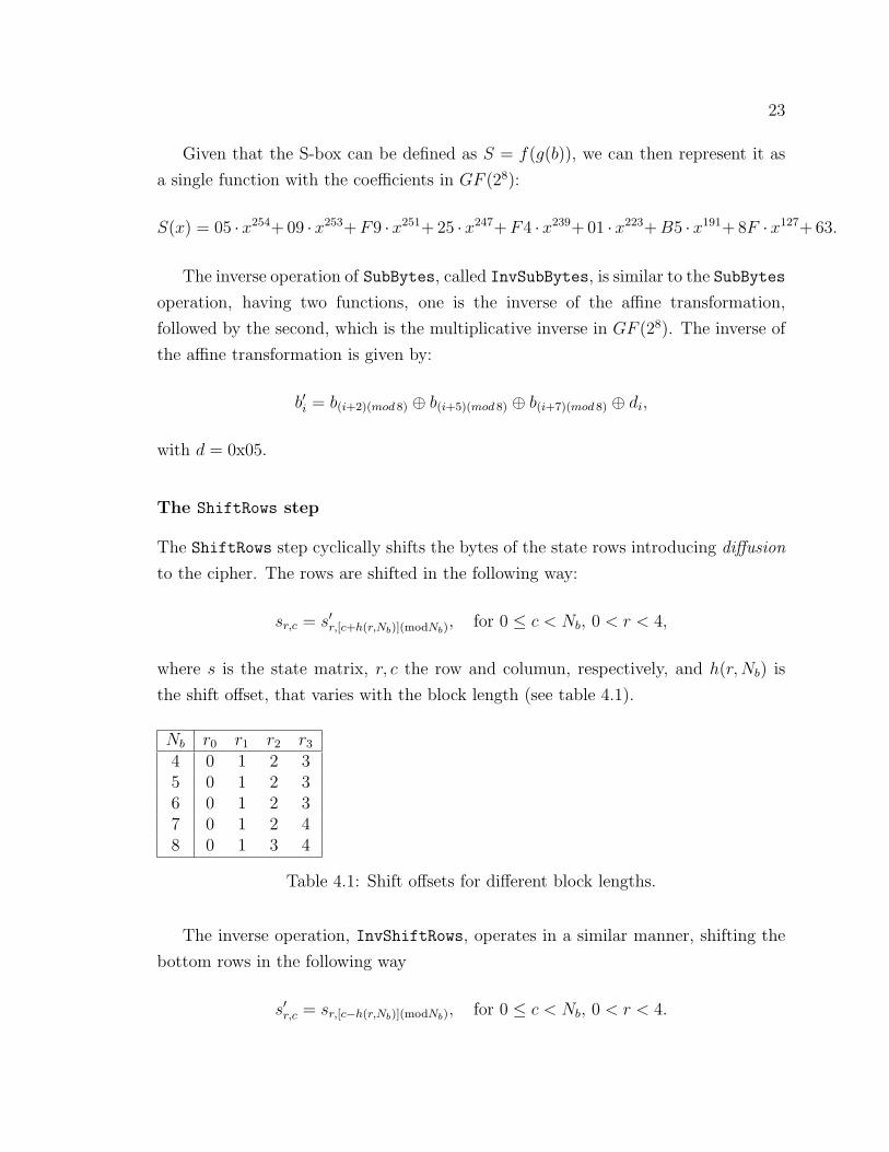
The ShiftRows step
The ShiftRows step cyclically shifts the bytes of the state rows introducing diffusion
to the cipher. The rows are shifted in the following way:
sr,c = s′r,[c+h(r,Nb)](modNb), for 0 ≤ c < Nb, 0 < r < 4,
where s is the state matrix, r, c the row and columun, respectively, and h(r,Nb) is
the shift offset, that varies with the block length (see table 4.1).
Nb r0 r1 r2 r3
4 0 1 2 35 0 1 2 36 0 1 2 37 0 1 2 48 0 1 3 4
Table 4.1: Shift offsets for different block lengths.
The inverse operation, InvShiftRows, operates in a similar manner, shifting the
bottom rows in the following way
s′r,c = sr,[c−h(r,Nb)](modNb), for 0 ≤ c < Nb, 0 < r < 4.

24
The MixColumns step
The MixColumns step operates independently on each of the state columns and
together with the ShiftRows step adds diffusion to the cipher. The columns of the
state are seen as polynomials over GF (28) and multiplied modulo x4 + 1 with a fixed
polynomial, c(x) = 03 ·x3 + 01 ·x2 +01 ·x + 02. This polynomial is coprime to x4 +1
and therefore invertible. Formally, we can define this step as a matrix multiplications′c,0
s′c,1
s′c,2
s′c,3
=
02 03 01 01
01 02 03 01
01 01 02 03
03 01 01 02
×sc,0
sc,1
sc,2
sc,3
.
This matrix is called maximum distance separable (MDS) matrix. The importance
of this matrices was studied by Vaudenay, on what he called multipermutations [47].
The corresponding inverse step, InvMixColumns, transforms the state columns in
similar manner as MixColumns
(03 · x3 + 01 · x2 + 01 · x + 02) · d(x) ≡ 01 (mod x4 + 1),
with d(x) given by
d(x) = 0B · x3 + 0D · x2 + 09 · x + 0E.
Written as a matrix multiplication, InvMixColumns, operates as followss′c,0
s′c,1
s′c,2
s′c,3
=
0E 0B 0D 09
09 0E 0B 0D
0D 09 0E 0B
0B 0D 09 0E
×sc,0
sc,1
sc,2
sc,3
.
The AddRoundKey step
This last step modifies the state by combining it with the round key derived via key
schedule, using the XOR operation. Due to the properties of XOR operation, the
inverse of AddRoundKey is AddRoundKey itself.

25
4.2.2 The Key Schedule
The key schedule responsability is to derive the ExpandedKey from the cipher key.
The ExpandedKey can be seen as a matrix Nb×(Nr+1), recalling that Nb is the block
length divided by 32 and Nr is the number of rounds. The ExpandedKey output is a
linear array of 4-byte words and is computed as follows: Let k0, ..., kNi−1denote the
first columns and let i ≥ Nk, then the following columns are computed recursively in
terms of previously defined columns in the following way:
1. If Nk 6| i, then column i is k[i] = k[i−Nk]⊕ k[i− 1];
2. If Nk | i, then the column i is k[i] = k[i−Nk]⊕SubWord(RotWord(k[i− 1]))⊕Rcon[i/Nk];
3. In case of Nk > 6 and i mod Nk is 4, then k[i] = k[i−Nk]⊕ SubWord(k[i− 1])
The | symbol denotes divisibility and consequently 6| denotes non-divisibility. The Sub-
Word functions takes as input a 4-byte word and applies the substitution of SubBytes
step to produce a 4-byte output word. The RotWord function takes as input a 4-byte
word and cyclically rotates bytes to the left, i.e., RotWord [b3, b2, b1, b0] = [b2, b1, b0, b3].
Finally, Rcon is a word array that contains the values [xi−1, 0, 0, 0], where xi−1 is a
member of the finite field of AES. After the computation of ExpandedKey, the round
key i consists of the words given by ExpandedKey[Nb ·i] to ExpandedKey[Nb ·(i+1)−1].
4.3 High-level implementation
The following high-level listings of the AES implementation were taken from [10].
Rijndael(State, CipherKey)
{
KeyExpansion(CipherKey, ExpandedKey);
AddRoundKey(State, ExpandedKey[0]);
for(i=1; i<$N_r$; i++) Round(State, ExpandedKey[i]);
FinalRound(State, ExpandedKey[$N_r$]);
}
Listing 1: AES encryption listing

26
Round(State, ExpandedKey[$i$])
{
SubBytes(State);
ShiftRows(State);
MixColumns(State);
AddRoundKey(State, ExpandedKey[$i$]);
}
FinalRound(State, ExpandedKey[$N_r$])
{
SubBytes(State);
ShiftRows(State);
AddRoundKey(State, ExpandedKey[$N_r$]);
}
Listing 2: AES round transformation
InvRound(State, ExpandedKey[$i$])
{
AddRoundKey(State, ExpandedKey[$i$]);
InvMixColumns(State);
InvShiftRows(State);
InvSubBytes(State);
}
InvFinalRound(State, ExpandedKey[$N_r$])
{
AddRoundKey(State, ExpandedKey[$N_r$]);
InvShiftRows(State);
InvSubBytes(State);
}
Listing 3: AES round transformation of the decryption algorithm

27
CHAPTER 5
CRYPTANALYSIS
Cryptanalysis, is the study, and analysis, of weaknesses and vulnerabilities found in
ciphers. The attacks performed against a cipher usually fit in one of the following
models [34]:
1. Ciphertext-only attack - the adversary tries to deduce the decryption key, or
plaintext, through the analyzes of the ciphertext.
2. Known-plaintext attack - the adversary possesses various plaintexts and the
corresponding ciphertexts, he or she tries do derive the key from those combi-
nations.
3. Chosen-plaintext attack - the adversary chooses plaintext and feeds it to the
cipher, obtaining this way the corresponding ciphertext. Subsequently, the
adversary tries to deduce any information of a previously unknown ciphertext.
4. Chosen-ciphertext attack - The attacker has the ability to provide a ciphertext
to the cipher and obtains the corresponding plaintext, under unknown key. The
objective is then to deduce the plaintext from another ciphertext.
We will focus on linear cryptanalysis [32], which is a known-plaintext attack, and
on differential cryptanalysis [3], which falls into the chosen-plaintext category.
5.1 Linear Cryptanalysis
The concept of linear cryptanalysis was first introduced by Matsui and Yamagishi
against FEAL [32] and later against DES [31]. It is a known-plaintext attack with
the finality of finding an approximate linear expression to the action of a cipher. This
method is also a statistical attack, meaning that, it is not guaranteed to work every
28
single case, but the probabilty of success can be increased if certain conditions (which
we will describe later) are met.
Linear cryptanalysis relies on the weaknesses of cipher structures, and on the
ideology that no cipher has perfect diffusion and confusion. Therefore, the mean to
achieve the purpose of the attack is to construct a statistical linear path between
input and output bits.
To construct such path, linear binary equations are used, this equations are on
the following format:
Pi1 ⊕ Pi2 ⊕ . . .⊕ Piu ⊕ Cj1 ⊕ Cj2 ⊕ . . .⊕ Cjv = 0
where Pi represents the i-th bit of the input P = [P1, P2, . . . , Pu] and Cj represents
the j-th bit of the output C = [C1, C2, . . . , Cj].
Ideally, a cipher should provide enough randomness so that an expression in the
above form would be true half of the time,i.e., by examining the output bits we
should see as many 0’s as 1’s. Linear cryptanalysis attemps to explore and determine
such expressions which have high or low probability of occurence - the probability of
getting a 0 or a 1 in the ouput is not 1/2, the further the deviation or bias is, the
better are the chances of a successful attack. To the amount of deviation in which the
probability of an expression differs from 1/2 we call linear probability bias. In other
words, if p is the probabilty of the above expression being true, then |p− 1/2| is the
linear probability bias, or simply bias.
The above equation could be reformulated as:
Pi1 ⊕ Pi2 ⊕ . . .⊕ Piu ⊕ Cj1 ⊕ Cj2 ⊕ . . .⊕ Cjv = Kk1 ⊕Kk2 ⊕ . . .⊕Kkw
where Kk represents the k-th bit of the unknown cipherkey K = [K1, K2, . . . , Kw]. If
the sum of the involved k bits is 0, the bias of the expression will have the same sign
as the expression involving the subkey sum, otherwise, it will have the opposite sign.
To construct such expressions with high linearity we must analyze the S-box of the
cipher, which is the only non-linear component. Once all the non-linear properties
of the S-box are analyzed we are able to start concatenating linear expressions of
the S-boxes so that the intermediate bits can be cancelled out and we are left with a
linear expression which as a large bias and involves bits from the plaintext and the last
29
round input. For a detailed analyze of this construction we refer to the outstanding
work of Heys [22].
Matsui describes two methods to mount a linear cryptanalysis attack, however,
only the method he calls ”Algorithm 2” [32] is widely used, hence that is the only
method we will describe. Both algorithms use the principle of maximum likelihood :
If it is the most probable cause, then we assume it is the correct cause.
Assuming we have an equation in the form above and large number of plaintext-
ciphertext pairs, under the key (we recall that this is a known-plaintext attack) we
wish to obtain. Also we must know the probability p that the equation holds true,
then:
1. 1 - For each set of key bits, we calculate the number of times the linear equation
holds true with the plaintext-ciphertext pairs. We denote this value by T .
2. 2 - We select the keys that are the farthest away from half the number of pairs.
That is, if N is the number of pairs we calculate |T − (N/2)| for each key.
The purpose of the above algorithm is to try all the values of key bits and find the
most likely set of them.
To make the life of cryptanlysts harder, the creators of AES studied a way to
prevent the cipher from falling victim to linear cryptanalysis. By analyzing the
properties of boolean functions they could represent those functions as correlation
matrices. The elements of these matrices consist of the correlation coefficients between
linear combinations of input bits and linear combinations of output bits, they serve as
a link between boolean mappings and linear mappings over specific linear functions,
thus, their importance to linear cryptanlysis [10].
For the linear cryptanalysis attack to be successful, the adversary must know the
correlation over all but a few rounds of the cipher with an amplitude slightly larger
than 2−nb/2. To avoid the attack the AES was designed with a number of rounds,
n−1k 2−nb/2, so that no correlation could be found. Also the key-schedule of AES, makes
the cipher strongly key-dependent, thus, making patterns for which high correlations
to occur highly infeasible.
30
5.2 Differential Cryptanalysis
Differential cryptanalysis was purposed by Biham and Shamir on [3] as an attack
against iterated cryptosystems, later, the same authors published the same attack
against DES [4]. The attack analyzes the results of particular differences on plain-
text pairs with the resultant ciphertext pairs. These differences are used to assign
probabilities to possible keys and find the most probable key, thus and like in linear
cryptanalysis, relying on the principle of maximum likelihood. Another similarity
with linear cryptanalysis is the already stated fact that this method is a probabilistic
attack. However, differential cryptanalysis is a chosen-plaintext attack, as opposed
to linear cryptanalysis, which is a known-plaintext attack and thus more realistic.
Differential cryptanalysis exploits the probability of determined occurences of
plaintext differences and ciphertext differences. Let us consider some system with
input P = [P1, P2, . . . , Pn] and output C = [C1, C2, . . . , Cn]. Let two inputs of that
system be P ′ and P ′′ with the corresponding outputs C ′ and C ′′. The input differences
is given by ∆P = P ′ ⊕ P ′′, and we can represent it as,
∆P = [∆P1,∆P2, . . . ,∆Pn]
where ∆Pi = ∆P ′i ⊕ ∆P ′′i with P ′i and P ′′i representing the i-th bit of P ′ and P ′′,
respectively.
In a similar way, the output differences is given by ∆C = C ′ ⊕ C ′′, and can be
denoted as,
∆C = [∆C1,∆C2, . . . ,∆Cn]
where ∆Ci = ∆C ′i ⊕∆C ′′i .
In a cipher with perfect randomization, we have that the probability of an ouput
difference ∆Y to occur given a particular input difference ∆P is 1/2n with n being
the number of bits of P . With this attack we try to find a pair (∆X,∆Y ) that occurs
with very high probability, p. To that pair we call differential.
Being a chosen-plaintext attack, the cryptanalyst (or the adversary) is able to
chose very specific inputs and obtain the corresponding outptus, hoping to derive the
key from further analyzes. Applied to differential cryptanalysis the attacker selects
pairs of inputs ∆P ′ and ∆P ′′, that satisfy a particular ∆P , with the knoweledge
that the correspoding output ∆C holds with high probability. The construction of

31
differentials is achieved through the analyzes of differential characteristics, which are
a sequence of input and output differences to the cipher rounds so that the output
difference from one round corresponds to the input difference for the next round.
In a smiliar way to linear cryptanalysis, the S-boxes must be examined but this
time we will be looking for the differences propagation properties. Then we can
combine the S-boxes difference pairs from one round to another in order that the
non-zero difference ouput bits from one round correspond to the non-zero difference
input bits of the next round, helps us in finding a highly probability differential
composed by the plaintext difference bits and the difference bits from the input to
the last round. For such construction we, again, referer to [22].
For the differential attack be successful, the cryptanalyst needs to know an input
difference pattern that propagates to an ouput difference pattern, over all but a few
of rounds of the cipher with a probability larger than 21−nb , hence, this was also took
in consideration while choosing the number of rounds of AES [10].

32
CHAPTER 6
CONCLUSIONS
6.1 What have we done so far?
In this thesis we covered the necessary tools to manipulate boolean functions and to
analyze their properties. We saw how important they are on the design of ciphers,
particularly on the design of S-boxes. We then explained how SAT solvers work and
how they can be applied to aid in the process of cryptanalysis. Finally, we gave an
insight on the design of AES, as well as, what keeps AES from being vulnerable to
linear and differential cryptanalysis.
6.2 Future directions
Since SAT solvers are getting to much attention, seems to us that the logic step to take
is to convert AES from GF (28) to GF (2)8, so we would have a boolean representation
of AES. In this way, we could then analyze its S-box and try simple attacks with the
SAT solver. A ”simple” attack could consist in solving the equation:
δ(S(x⊕ k) + y) = 1
where δ is the Kronecker delta, described in chapter 2, x is the input bits and y the
ouput bits after the inputs bits being XOR’ed with the key, k and being fed to the
S-box, S. We could the try to extend this attack to more than one round.
Another application of SAT solvers in the cryptanalysis of AES, could be the
study of correlation matrices and the differences propagation on the S-boxes.

33
REFERENCES
[1] Advanced Encryption Standard (AES). Federal Information Processing Stan-dards Publication 197. National Institute of Science and Technology, 2001.
[2] R.J. Bayardo and R.C. Schrag. Using CSP look-back techniques to solve real-world SAT instances. In Proceedings of the National Conference on ArtificialIntelligence, pages 203–208. JOHN WILEY & SONS LTD, 1997.
[3] E. Biham and A. Shamir. Differential cryptanalysis of DES-like cryptosystems.Journal of CRYPTOLOGY, 4(1):3–72, 1991.
[4] E. Biham and A. Shamir. Differential cryptanalysis of the full 16-round DES.Lecture Notes in Computer Science, pages 487–487, 1993.
[5] C. Cid, S. Murphy, and M. Robshaw. Algebraic aspects of the advanced encryp-tion standard. Springer Verlag, 2006.
[6] N.T. Courtois and G.V. Bard. Algebraic cryptanalysis of the data encryptionstandard. Lecture Notes in Computer Science, 4887:152, 2007.
[7] N.T. Courtois, G.V. Bard, and A. Bogdanov. Periodic ciphers with small blocksand cryptanalysis of keeloq. Tatra Mountains Mathematical Publications, 2008.
[8] N.T. Courtois, K. Nohl, and S. O’Neil. Algebraic attacks on the crypto-1 streamcipher in mifare classic and oyster cards. Early announcement of a research inprogress, 14, 2008.
[9] N.T. Courtois and J. Pieprzyk. Cryptanalysis of block ciphers with overdefinedsystems of equations. Lecture Notes in Computer Science, 2501:267–287, 2002.
[10] J. Daemen and V. Rijmen. The Design of Rijndael: AES–the Advanced Encryp-tion Standard. Springer, 2002.
[11] M. Davis and H. Putnam. A computing procedure for quantification theory.Journal of the ACM, 7(3):201–215, 1960.
[12] Martin Davis, George Logemann, and Donald Loveland. A machine program fortheorem-proving. Commun. ACM, 5(7):394–397, 1962.
34
[13] D. De, A. Kumarasubramanian, and R. Venkatesan. Inversion attacks on securehash functions using SAT solvers. Lecture Notes in Computer Science, 4501:377,2007.
[14] Data Encryption Standard (DES). Federal Information Processing StandardsPublication 46. National Institute of Science and Technology, 1977.
[15] H. Dobbertin. Cryptanalysis of MD4. Journal of Cryptology, 11(4):253–271,1998.
[16] N. Een and N. Sorensson. An extensible SAT-solver. Lecture notes in computerscience, 2919:502–518, 2004.
[17] N. Een and N. Sorensson. MiniSat: A SAT solver with conflict-clause minimiza-tion. 8th SAT, 2005.
[18] C. Fiorini, E. Martinelli, and F. Massacci. How to fake an RSA signature byencoding modular root finding as a SAT problem. Discrete Applied Mathematics,130(2):101–127, 2003.
[19] B. Gladman. A specification for Rijndael, the AES algorithm.http://www.techheap.com/cryptography/encryption/spec.v36.pdf.
[20] E. Goldberg and Y. Novikov. BerkMin: A fast and robust SAT-solver. DiscreteApplied Mathematics, 155(12):1549–1561, 2007.
[21] C.P. Gomes, B. Selman, and H. Kautz. Boosting combinatorial search throughrandomization. In Proceedings of the National Conference on Artificial Intelli-gence, pages 431–437. JOHN WILEY & SONS LTD, 1998.
[22] H.M. Heys. A tutorial on linear and differential cryptanalysis. Cryptologia,26(3):189–221, 2002.
[23] N. Jacobson and N. Jacobson. Basic algebra. WH Freeman San Francisco, 1974.
[24] D. Jovanovic and P. Janicic. Logical analysis of hash functions. Lecture notes incomputer science, 3717:200, 2005.
[25] R. Lidl and H. Niederreiter. Introduction to finite fields and their applications.Cambridge University Press, 1986.
[26] J. Marques-Silva. The impact of branching heuristics in propositional satisfia-bility algorithms. Lecture notes in computer science, pages 62–74, 1999.
[27] JP Marques-Silva and KA Sakallah. GRASP: A search algorithm for proposi-tional satisfiability. IEEE Transactions on Computers, 48(5):506–521, 1999.

35
[28] F. Massacci. Using Walk-SAT and Rel-SAT for cryptographic key search. InInternational Joint Conference on Artificial Intelligence, volume 16, pages 290–295. LAWRENCE ERLBAUM ASSOCIATES LTD, 1999.
[29] F. Massacci and L. Marraro. Logical cryptanalysis as a SAT problem. Journalof Automated Reasoning, 24(1):165–203, 2000.
[30] F. Massacci and L. Marraro. Logical cryptanalysis as a SAT problem. Journalof Automated Reasoning, 24(1):165–203, 2000.
[31] M. Matsui. Linear cryptanalysis method for DES cipher. Lecture Notes inComputer Science, 765:386–397, 1994.
[32] M. Matsui and A. Yamagishi. A new method for known plaintext attack of FEALcipher. Lecture Notes in Computer Science, pages 81–81, 1993.
[33] R.J. McEliece. Finite fields for computer scientists and engineers. Springer,1987.
[34] A.J. Menezes, P.C. Van Oorschot, and S.A. Vanstone. Handbook of appliedcryptography. CRC press, 1997.
[35] I. Mironov and L. Zhang. Applications of SAT solvers to cryptanalysis of hashfunctions. Lecture Notes in Computer Science, 4121:102, 2006.
[36] S. Mister and C. Adams. Practical S-box design. In Workshop on Selected Areasin Cryptography, SAC, volume 96, pages 61–76. Citeseer, 1996.
[37] MW Moskewicz, CF Madigan, Y. Zhao, L. Zhang, and S. Malik. Chaff:Engineering an efficient SAT solver. In Design Automation Conference, 2001.Proceedings, pages 530–535, 2001.
[38] P. Prosser. Hybrid algorithms for the constraint satisfaction problem. Compu-tational intelligence, 9(3):268–299, 1993.
[39] B. Selman, H. Kautz, and B. Cohen. Local search strategies for satisfiabilitytesting. DIMACS Series in Discrete Mathematics and Theoretical ComputerScience, 1993.
[40] B. Selman, H. Levesque, and D. Mitchell. A new method for solving hardsatisfiability problems. In Proceedings of the Tenth National Conference onArtificial Intelligence, pages 440–446, 1992.
[41] C. Shannon. Communication theory of secrecy systems. Bell Systems Technical.Journal, 28:656–715, 1949.

[42] M. Soos, K. Nohl, and C. Castelluccia. Extending SAT Solvers to CryptographicProblems. In Proceedings of the 12th International Conference on Theory andApplications of Satisfiability Testing, page 257. Springer, 2009.
[43] D. Sterndark. The RC4 encryption algorithm.http://groups.google.com/group/sci.crypt/msg/10a300c9d21afca0, 1994.
[44] Y. Tarannikov. On Correlation Immune Boolean Functions. In Boolean Functionsin Cryptology and Information Security, volume 18, pages 219–231. NATO-Russia Advanced Study Institute, 2008.
[45] G.S. Tseitin. On the complexity of derivation in propositional calculus. Studiesin constructive mathematics and mathematical logic, 2(115-125):10–13, 1968.
[46] J. Valenca. Tecnincas Criptograficas, 2008.
[47] S. Vaudenay. On the need for multipermutations: Cryptanalysis of MD4 andSAFER. Lecture Notes in Computer Science, pages 286–286, 1995.
[48] AF Webster and S.E. Tavares. On the design of S-boxes. In Advances inCryptology-CRYPTO, volume 85, pages 523–534. Citeseer, 1986.
[49] SB Xu, DK He, and XM Wang. An Impelementation of the GSM General DataEncryption Algorithm A5. CHIANCRYPT94, pages 11–15, 1994.
[50] H. Zhang. SATO: An efficient propositional prover. Lecture Notes in ComputerScience, 1249:272–275, 1997.