A Study on Carbon Reduction in the Vehicle

Routing Problem with Simultaneous Pickups and

Deliveries

Yixiao Huang, Chunyang Shi, Lei Zhao

Department of Industrial Engineering

Tsinghua University, Beijing, China

Tom Van Woensel

School of Industrial Engineering

Eindhoven University of Technology, Eindhoven, The Netherlands

Abstract-Reducing greenhouse gases (GHG), especially car­bon dioxide, has become a critical environmental issue worldwide and has attracted attentions in all economic sectors and indus­tries. Ranking the second in cargo turnover volume in China, road cargo transportation has become a key carbon reduction field in the country. In this paper, we study the vehicle routing problem with simultaneous pickups and deliveries (VRPSPD), a commonly encountered practice in road cargo transportation, especially associated with reverse logistics. More specifically, we study a green VRPSPD (g-VRPSPD) problem by including fuel consumption and carbon emission costs into the model. Our numerical results show that, comparing with the traditional distance-minimizing model, the proposed g-VRPSPD model can generate more environment-friendly routes without scarifying much on the total travel distance. We also provide guidelines for green vehicle routing strategies.

I. INTRODUCTION

Greenhouse gases (GHG) reduction has become an im­

portant issue due to global warming, especially in freight

transportation. According to the World Resources Institute

(WRI, http://www.wri.org/).in 2005, the transportation sector

accounts for 14.3%, among which road transportation accounts

for 10.5%, of the world greenhouse gas emissions. In the

United States, the transportation sector contributes 28% of the

country's overall GHG emissions [1]. In the United Kingdom,

21 % of the CO2 emissions of the transportation sector is

from freight transportation, which accounts for 6% of the

C02 emissions in the country [2]. In China, the road cargo

transportation ranks the second in the country's cargo turnover

volume.

In reverse logistics, vehicles may pick up and deliver goods

at the same time. For products to be recycled or reproduced,

vehicles may deliver new products to customers while picking

up the recycled ones from customers in one route, to increase

vehicle utilization and reduce travel milage, and therefore save

overall operational cost.

The vehicle routing problem with simultaneous pickups

and deliveries (VRPSPD) is a variant of the classical vehicle

routing problem (VRP), where pickup and delivery demand

978-1-4673-2401-4112/$3l.00 ©2012 IEEE

may appear at the same customer node. Moreover, all pickups

are collected at the depot and all deliveries originate from the

depot. In this paper, we study a green VRPSPD (g-VRPSPD)

problem, by considering fuel consumption and carbon e­

missions. We formulate a two-index commodity flow based

linear integer programming model for VRPSPD, modified

from Montane and Galvao [3]. We then perform numerical

experiments based on a real world case of a logistics company

in Europe. The numerical results indicate that, comparing with

the traditional distance-minimizing model, the g-VRPSPD

model can generate more environment-friendly routes without

scarifying much on the total travel distance.

The rest of the paper is organized as follows. Section II

reviews the relevant literature. Section III describes the green

VRPSPD problem and the linear integer programming model.

In Section IV, we describe the numerical experiments and

analysis, and provide guidelines for green vehicle routing

strategies. Section V concludes the paper.

II. LITERATURE REVIEW

The vehicle routing problem was introduced by Dantzig and

Ramser [4]. Since then variants of VRP have been studied

for various situations in transportation. Min [5] recognizes

the possibility of simultaneous pickup and delivery at the

same node in practical situations and introduces the vehicle

routing problem with simultaneous pickups and deliveries

(VRPSPD). Montane and Galvao propose a commodity flow

based model for VRPSPD [3]. Based on the commodity

flow model, Dell' Amico et al. [6] develop a branch-and-price

approach to solve VRPSPD exactly for small to medium

size instances. For large-scale VRPSPD problems, research

has been focusing on heuristic and meta-heuristic methods.

Dethloff [7] studies the cheapest insertion with four different

insertion criteria: travel distance (TD), residual capacity (RC),

and radial surcharge (RS) and their combination (RCRS).

Nagy and Salhi [8] develop mathematical relationships to

describe how route changes affect solution feasibility, based

on which they propose an integrated heuristic method to solve

302

the VRPSPD. It first finds a solution to the corresponding VRP

and modifies the solution to make it feasible for the VRPSPD.

They then apply composite improvement heuristics to improve

the solution. Chen and Wu [9] apply the cheapest insertion

heuristic to construct an initial solution and then improve the

solution based on the record-to-record travel, tabu lists, and

route improvement procedures. Bianchessi and Righini [10]

present and compare a variety of constructive, local search,

and tabu search algorithms via numerical experiments.

Due to the importance of reduction on carbon emissions and

fuel consumption in transportation, in recent years there have

been studies linking fuel consumption and carbon emissions

with the vehicle routing problem and its variants. Bektas and

Laporte [2] use the comprehensive modal emission model (de­

veloped by Barth et al. [11]) to include fuel consumption and

carbon emissions in the capacitated vehicle routing problem

and the variant with time windows (VRP TW ). Xiao et al. [12]

add the load dependent fuel consumption rate (FCR) into the

capacitated VRP, and develop a simulated annealing algorithm

with a hybrid exchange rule to solve the problem. Their

numerical experiments show that the proposed model can

result in 5% fuel consumption savings on average as compared

to the traditional CVRP model. Kuo [13] use the simulated

annealing approach to minimize fuel consumption in the time­

dependent vehicle routing problem (TDVRP ). Figliozzi [14]

analyzes C02 emissions for different levels of congestion

and time-definitive customer demands, using travel time data

from an extensive archive of freeway sensors, time-dependent

VRP algorithms, etc. Ubeda et al. [15] use a case study on

a leading company in the Spanish food distribution sector to

test the green logistics initiative in practice by incorporating

environmental criteria into the vehicle routing problem and

the variant with backhauls (VRPB). Erdogan and Miller-Hooks

[1] study the capacitated vehicle routing problem with vehicles

using alternative fuel and therefore subjective to travel distance

constraint between refills.

In VRPSPD, the vehicle load is no longer monotonously

increasing (as in the pure pickup case) or decreasing (as in

the pure delivery case). This characteristic complicates, but

on the other hand offers more flexibility on, routing decisions.

In this paper, we study the green VRPSPD (g-VRPSPD)

problem, where we incorporate fuel consumption and carbon

emissions into the VRPSPD model. To the best of the authors'

knowledge, there has been no prior research on this subject.

III. MATHEMATICAL MODEL

In this section, we describe the g-VRPSPD problem and

introduces its mathematical formulation.

A. Problem Description

In the VRPSPD, we manage a fleet of K homogeneous

vehicles and design optimal routes to serve a set of customers

from a central depot. On the distribution network, G = (V, A), V = {O, 1, ... , n} is the set of n + 1 nodes, where node 0

represents the depot and other nodes represent customer nodes,

and A = {( i, j) : i, j E V, i =J j} is the set of directed arcs

in the network. A distance matrix Dij is defined on A. At

each node i, the customer may have pickup demand Pi, or

delivery demand di, or both. The capacity of each vehicle is

Q. As in the classical VRP setting, each vehicle should start

its tour from the depot and return to the depot at the end of

the tour. Each customer is visited exactly once by one vehicle.

We assume that the capacity of vehicles can at least satisfy

the demand of each customer.

In addition to minimizing the distance-related cost and setup

cost of vehicles as in the traditional VRPSPD model, the g­

VRPSPD problem also includes the costs of fuel consumption

and carbon emissions in the objective function. Similar to [12],

we assume that fuel consumption and carbon emissions are

proportional to the driving distance and linear with the vehicle

load. That is,

fuel consumption = (a x 10-3 x load + b) x distance, (1)

and

carbon emissions = f..L x fuel consumption, (2)

where a and b are the coefficients of vehicle fuel consumption

and f..L is the emission rate of fuel consumption.

B. An Linear Integer Programming Formulation

For the ease of incorporating fuel consumption and carbon

emissions in VRPSPD, we choose the commodity flow based

model in which the vehicle load is explicitly expressed. We

modify the commodity flow model of [3] for the g-VRPSPD

problem as follows.

Let Xij be the binary variable to indicate whether arc (i, j) is visited on the route. Yij denotes the demand picked up from

customers routed up to node i and transported on arc (i, j); Zij denotes the demand to be delivered to customers routed

after node i and transported on arc (i, j). With the vehicle

load variables Yij and Zij, the fuel consumption from node i to node j can be calculated as Dij[a(Yij + Zij) + b], and the

carbon emissions can be calculated as f..LDij [a(Yij + Zij) + b]. Let Cd denote the unit distance-related cost, Cv denote

the setup cost of a vehicle, cf denote the unit fuel cost,

and Ce denote the environmental cost of carbon emissions.

The mathematical model of g-VRPSPD can be formulated as

below.

s.t.

303

min

Cd L L DijXij + Cf L L DijXij[a(Yij + Zij) + b] iEV JEV iEV JEV

+ cef..L L L DijXij [a(Yij + Zij) + b] + Cv L XOj iEV JEV JEV\ {O}

L Xij = 1, Vj E V \ {O}, iEV

L Xij = 1, Vi E V \ {O}, JEV

(3)

(4)

(5)

L XiO:S; K, iEV

(6) We observe that constraints (11) assure that Yij and Zij are

L XOj = L XiO, JEV iEV

Xij + Xji :s; I, Vi,j E V \ {O}, i < j,

L Yjm - L Yij =Pj, mEV iEV

Vj E V \ {O},

L Zij - L Zjm = dj, Vj E V\ {O}, iEV mEV

Yij + Zij :s; QXij, Vi, j E V,

YOj = 0, j E V \ {O},

(7)

(8)

(9)

(10)

(11)

(12)

positive only if Xij = 1. Therefore, we can convert the bilinear

objective function into the equivalent linear form (20).

min

iEV JEV iEV JEV

+ CeIL L L Dij[a(Yij + Zij) + b] + Cv L XOj· (20) iEV JEV jEV\{O}

IV. COMPUTATIONAL EXPERIMENTS

We choose the real world case of a logistics company in

Europe, with one depot and around 70 customers with pickup

and/or delivery demand. The firm operates a homogeneous

fleet of heavy diesel vehicles with capacity of 24 tons. Every

3 working days, the firm assigns vehicles to visit a subset of

customers, based on their demand.

L YiO = L Pi, (13) A. Test Instances iEV\ {O} iEV\ {O}

ZiO = 0, Vi E V \ {O},

L ZOj = L dj, jEV\ {O} jEV\ {O}

Yij ;::: PiXij, Vi E V \ {O}, Vj E V,

Zij ;::: djXij, Vi E V, Vj E V \ {O},

Xij E {O, I}, i,j E V,

Yij, Zij ;::: 0, i, j E V.

(14)

(15)

(16)

(17)

(18)

(19)

The objective function (3) consists of both economic cost

(distance-related cost and setup cost of vehicles) and en­

vironmental (fuel consumption and carbon emissions) cost.

Constraints (4) and (5) ensure that each customer node is

visited exactly once. Constraint (6) enforces the fleet size

constraint, i.e., the number of vehicles used should not exceed

K. Constraint (7) is the flow balance constraint at the depot.

Constraints (8) eliminate the two-node subtours. Constraints

(9) and (10) ensure that the demand of pickups and deliveries

at each node is satisfied. Constraints (11) guarantee that the

vehicle load should not exceed vehicle capacity. Constraints

(12) indicate no demand is picked up when vehicles leave the

depot. Constraint (13) assures all pickup demand is transported

from customer nodes to the depot. Constraints (14) indicate all

delivery demand is satisfied when vehicles return to the depot.

Constraint (15) assures all delivery demand is transported out

of the depot. Constraints (16) restrict the load of pickup in the

vehicle is not less than the pickup demand of the customer

node just visited. Constraints (17) restrict that the load of

delivery in the vehicle is not less than the delivery demand

of the customer node to be visited. Constraints (18) define the

binary variables Xij and constraints (19) ensure Yij and Zij are nonnegative.

We denote Kmin as the minimium number of vehicles re­

quired to serve the customer demand, which can be calculated

as

Kmin = max{lLiEV�{O} Pi

l, ILiEV�{O} di

U

The average vehicle load W can be estimated as

W = LiEV\{O} Pi + LiEV\{O} di

2Kmm

(21)

(22)

To better understand the 10 test instances, we list their

characteristics in Table I: the number of customers, average

distance, range of distance, and average vehicle load. The

average distance refers to the average distance of the Dij matrix, and the range of distance refers to the range of the

Dij matrix.

TABLE I INSTANCE CHARACTERISTICS

# of Average Range of Average customers distance distance load

20 306 701 16.6 20 279 697 13.7 20 294 684 17.6 20 278 776 13.1 22 284 622 17.9 24 295 776 16.2 20 272 622 18.8 24 285 697 19.1 23 297 774 15.1 20 313 698 14.9

In the numerical experiments, we compare models with

different objective functions. In the traditional distance­minimizing model, we ignore the fuel consumption and carbon

emission costs (cf = Ce = 0). In the emission-minimizing model, we ignore the distance and fuel consumption costs

(Cd = cf = 0). In the cost-minimizing model, the objective

function includes distance related cost as well as fuel con­

sumption and carbon emission costs.

304

The cost coefficients are calculated as follows. In all cases, the setup cost of vehicles Cv are set to be sufficiently large to assure the number of vehicles is minimal. The cost of a 24-ton-capacity vehicle is €70,000. The mileage is expected to be 400,000 kilometers. Then Cd = 70,000/400,000 =

€0.175/km. We set cf = €1.2/liter according to the diesel price on March 30th, 2011 I. Based on the report of Depart­ment for Environment, Food and Rural Affairs (DEFRA) in the UK [16], it suggests that £27 It of CO2 emitted in year 2010, with a 2% increase each year. We use the exchange rate £1 = €1.134 on March 30th, 201l. We obtain Ce =

27 x 1.02 x 1.134/1,000 = €0.031/kg. For the type of vehicle, it consumes 36.08 liters of fuel in

full load, 28.84 liters in 50% load, 21.18 liters in empty load. With linear regression we obtain the function

Fuel consumption = (6.208 x 10-3 x load+0.2125) x distance (23)

We then set a = 6.208 x 10-3 and b = 0.2125. The value of emission rate f-L = 2.68 referring to operation data of the company.

B. Comparison among Different Models

We solve the instances optimally with Xpress-MP and show the comparative results in Fig. l. We use the objec­tive function values of the distance-minimizing model as the benchmark, and compare it with the emission-minimizing and cost-minimizing models on total cost, travel distance, and carbon emissions.

6.0% 10 Cost-minimizing model

I 10 Emis sion-nUnimizing model

4.0%

� � 2.0%

0.0%

-2.0%

-4 .0% Cost reduction Dist. reduction Carbon reduction

Fig. 1. Comparison statistics, benchmarking with the distance-minimizing

model

We observe that the emission-minimizing model and the cost-minimizing model have the similar results. Compared with the traditional distance-minimizing model, the emission­minimizing model can reduce carbon emissions 4.2% on average and 6.5% at most, save total cost 2.4% on average, while only increasing distance by l.8% on average. That is, comparing with the traditional distance-minimizing model, the

1 http://gasoline-germany.comlinternational.phtml

proposed g-VRPSPD model can generate more environment­friendly routes without scarifying much on the total travel distance. These results agree with the observations made by Bektas and Laporte [2]. In the following sections, we focus on the comparison between the emission-minimizing and distance-minimizing models.

C. Parameter Analysis

Next, using the instances in Section IV-B as baseline, we vary parameters to study certain factors that may affect the impact of the g-VRPSPD model on carbon emissions.

When the fuel consumption rate b decreases, the relative effect of travel distance to vehicle load decreases, as shown in the fuel consumption calculation, Dij [a(Yij + Zij) + b]. When we reduce the b value from 0.2125 to 0.1063, the routing decisions of the distance-minimizing model remain the same, while the emission-minimizing model tends to select routes with longer distance but with much fewer carbon emissions. Consequently, the reduction of carbon emissions (distance­minimizing model vs. emission-minimizing model) improves from 4.2% (baseline result) to 7.3% on average (Fig. 2) but the increase in distance changes from l.8% to 2.9%. That is, when the fuel consumption rate becomes smaller, the emission­minimizing model has more significant impact on carbon emission reduction than the traditional distance-minimizing model, while resulting in longer total travel distance.

10.0% 9.0%

...... 8.0% c 2 7.0% '" 0.. 6.0%

£ 5.0% c .,g 4.0% " :::l ." '" 3.0% r<: 2.0%

10% r 0.0% .L.I._....LII"--....... _ ..... --'-....... -'-'''--....... '--..... --' _________ _ 10

Instance .Baseline instances • Instances with smaller b

Fig. 2. Effect of b on carbon emission reduction

The average distance between nodes indicates the geograph­ic scale of the network, that is, the larger the average distance, the customer nodes are farther away from each other. When we increase the average distance from 290 to 590 kilometers, the reduction of carbon emissions (the emission-minimizing model vs. the distance-minimizing model) improves from 4.2% to 5.1% on average (Fig. 3). On the other hand, the increase in distance reduces from l.8% to l.6%. It shows that, when the average distance increases, the vehicle load will have more significant impact on fuel consumption and therefore carbon emissions. Thus, the emission-minimizing model has more significant impact on carbon emission reduction in more

305

geographically scattered networks without sacrificing much in logistics managers to choose among models in their green fleet

total travel distance, as compared to the distance-minimizing management.

model.

8.0%

7.0%

C 6.0% " � " 5.0% Q. »

.D 4.0% c

. � 3.0% u

� " 2.0% �

1.0%

0.0% [ 10

Instance • Baseline Instances

• Instances with larger average distance

Fig. 3. Effect of average distance on carbon emission reduction

The range of distance indicates the variability in distances

between customer nodes in the network. When the range

of distance decreases, vehicles have more routing choices

without significant changes in the distance, while some routes

may reduce more carbon emissions. We decrease the range

of distance from 705 to 353 kilometers, the reduction of

carbon emissions (the emission-minimizing model vs. the

distance-minimizing model) improves from 4.2% to 5.0% on

average (Fig. 4), while the increase in distance reduces from

1.8% to 1.5%. That is, when the variability in distances in

the network is smaller, the emission-minimizing model has

more significant impact on carbon emission reduction without

sacrificing much in total travel distance, as compared to the

distance-minimizing model.

7.0%

6.0%

c � 5.0% " Q. � 4.0%

.D c

.� 3.0% u

" .", 2.0% " �

1.0%

0.0% 10

Instance

_Baseline instances

• Instances with smaller distance range

Fig. 4. Effect of distance range on carbon emission reduction

Based on the above observations, we understand that the

fuel consumption efficiency and the network structure both

affect the relative impact of different models on carbon e­

mission reduction, which can help to provide guidelines for

D. Guidelines for Emission-Saving Routing

Based on the observations on the results of different models,

we provide some guidelines for real world fleet management

or vehicle routing.

1) In green vehicle routing, vehicles should visit customers

with delivery demand before customers with pickup

demand, to decrease the average load of vehicles .

2) In green vehicle routing, vehicles visit customers with

delivery demand in descending order and customers with

pickup demand in ascending order. Combining with the

first guideline, vehicles should serve the large delivery

demand earlier in the route and large pickup demand

later in the route. With possible increase in total travel

distance, these two guidelines aim to reduce the average

load of vehicles.

3) In green vehicle routing, vehicles are assigned in bal­

anced loads and travel distances. Comparing Fig. 5(a)

(distance-minimizing routes) and Fig. 5(b) (emission­

minimizing routes), the latter generates more balanced

routes and therefore reduces the overall ton-milage,

which in turn reduces fuel consumption and carbon

emiSSIOns.

(a) The distance-minimizing routes

(b) The emission-minimizing routes

Fig. 5. Guideline for green routing: balanced routing

V. CONCLUSIONS

Different from other VRP variants, the non-monotone ve­

hicle loads on route in VRPSPD results in complexity, yet

306

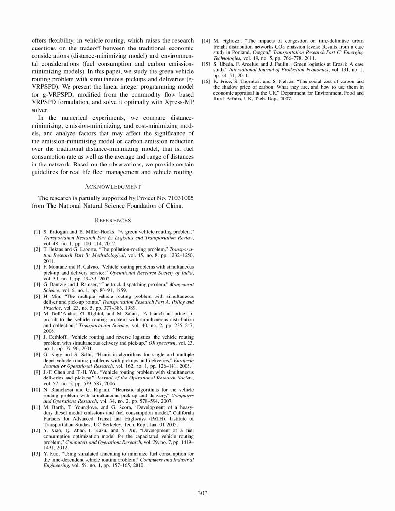
offers flexibility, in vehicle routing, which raises the research

questions on the tradeoff between the traditional economic

considerations (distance-minimizing model) and environmen­

tal considerations (fuel consumption and carbon emission­

minimizing models). In this paper, we study the green vehicle

routing problem with simultaneous pickups and deliveries (g­

VRPSPD). We present the linear integer programming model

for g-VRPSPD, modified from the commodity flow based

VRPSPD formulation, and solve it optimally with Xpress-MP

solver.

In the numerical experiments, we compare distance­

minimizing, emission-minimizing, and cost-minimizing mod­

els, and analyze factors that may affect the significance of

the emission-minimizing model on carbon emission reduction

over the traditional distance-minimizing model, that is, fuel

consumption rate as well as the average and range of distances

in the network. Based on the observations, we provide certain

guidelines for real life fleet management and vehicle routing.

ACKNOWLEDGMENT

The research is partially supported by Project No. 71031005

from The National Natural Science Foundation of China.

REFERENCES

[1] S. Erdogan and E. MiUer-Hooks, "A green vehicle routing problem," Transportation Research Part E: Logistics and Transportation Review, vol. 48, no. 1, pp. 100-ll4, 2012.

[2] T Bektas and G. Laporte, "The pollution-routing problem," Transporta­

tion Research Part B: Methodological, vol. 45, no. 8, pp. 1232-1250, 2011.

[3] F. Montane and R. Galvao, "Vehicle routing problems with simultaneous pick-up and delivery service," Operational Research Society of India,

vol. 39, no. 1, pp. 19-33, 2002. [4] G. Dantzig and J. Ramser, 'The truck dispatching problem," Mangement

Science, vol. 6, no. 1, pp. 80-91, 1959. [5] H. Min, "The multiple vehicle routing problem with simultaneous

deliver and pick-up points," Transportation Research Part A: Policy and

P ractice, vol. 23, no. 5, pp. 377-386, 1989. [6] M. Dell' Amico, G. Righini, and M. Salani, "A branch-and-price ap­

proach to the vehicle routing problem with simultaneous distribution and collection," Transportation Science, vol. 40, no. 2, pp. 235-247, 2006.

[7] J. Dethloff, "Vehicle routing and reverse logistics: the vehicle routing problem with simultaneous delivery and pick-up," OR spectrum, vol. 23, no. 1, pp. 79-96, 200 l.

[8] G. Nagy and S. Salhi, "Heuristic algorithms for single and multiple depot vehicle routing problems with pickups and deliveries," European

Journal of Operational Research, vol. 162, no. 1, pp. 126-141, 2005. [9] J.-F. Chen and T-H. Wu, "Vehicle routing problem with simultaneous

deliveries and pickups," Journal of the Operational Research Society,

vol. 57, no. 5, pp. 579-587, 2006. [10] N. Bianchessi and G. Righini, "Heuristic algorithms for the vehicle

routing problem with simultaneous pick-up and delivery," Computers

and Operations Research, vol. 34, no. 2, pp. 578-594,2007. [11] M. Barth, T Younglove, and G. Scora, "Development of a heavy­

duty diesel modal emissions and fuel consumption model," California Partners for Advanced Transit and Highways (PATH), Institute of Transportation Studies, UC Berkeley, Tech. Rep., Jan. 01 2005.

[l2] Y. Xiao, Q. Zhao, I. Kaku, and Y. Xu, "Development of a fuel consumption optimization model for the capacitated vehicle routing problem," Computers and Operations Research, vol. 39, no. 7, pp. 1419-1431, 2012.

[13] Y. Kuo, "Using simulated annealing to minimize fuel consumption for the time-dependent vehicle routing problem," Computers and Industrial

Engineering, vol. 59, no. 1, pp. 157-165, 2010.

[14] M. Figliozzi, "The impacts of congestion on time-definitive urban freight distribution networks C02 emission levels: Results from a case study in Portland, Oregon," Transportation Research Part C: Emerging

Technologies, vol. 19, no. 5, pp. 766-778, 2011. [l5] S. Ubeda, F. Arcelus, and J. Faulin, "Green logistics at Eroski: A case

study," International Journal of P roduction Economics, vol. 131, no. 1, pp. 44-51, 2011.

[l6] R. Price, S. Thornton, and S. Nelson, 'The social cost of carbon and the shadow price of carbon: What they are, and how to use them in economic appraisal in the UK," Department for Environment, Food and Rural Affairs, UK, Tech. Rep., 2007.

307