
Reviews Cameras Buying Guide Canon EOS 20D Review, Phil Askey
description

APPENDIX D
GROUNDWATER AVAILABILITY GAM ANALYSES

Intera Incorporated 1812 Centre Creek Drive, Suite 300 Austin, Texas 78754 Telephone: 512 425 2000 Fax: 512 425 2099
M E M O R A N D U M
To: PWPG Modeling Committee From: Van Kelley, INTERA Dennis Fryar, INTERA Neil Deeds, INTERA Date: November 11, 2009 RE: Regional Availability and Available Supplies: Current GAM In the planning group meeting held July 14th in Amarillo, it was determined that the draft groundwater planning numbers would be based upon the current GAM, with updated estimates being included in a later draft after the GAM is revised. In a modeling committee meeting held August 7th in Amarillo, the simulations desired by the planning group were defined. It was the intention of the group that each of these simulations be available using both the current Dutton (2004) GAM and the revised GAM being developed by INTERA. The three simulation types requested include; the Baseline Demand simulation (Baseline); the Regional Availability simulation, and the Available Supplies simulation. As defined by GMA 1, these are to be simulated using both the current GAM and the future revised GAM. Table 1 provides a summary of each of these three simulation types in terms of purpose, approach, and results. This memorandum documents the Regional Availability Simulation and the Available Supplies Simulation for the current GAM. Table 1. Scope of simulations requested by the planning group.
Simulation Purpose Approach Expected Results Baseline
(Includes updated demands)
Estimate groundwater availability with current pumping locations
Use current pumping locations and projected use
Capability to meet demands with current infrastructure – areas of concern
Regional Availability (MAG)
Determine available groundwater given regional management goals
Approach employed in GAM Run 09-001 except to correct pumping annually to meet goals
Theoretical availability assuming management at the one-square mile level
Available Supplies Estimate groundwater available to each user groups
Refined approach to GAM Run 09-001 with management areas defined by dominant user groups
Available supplies to be used in the needs analysis and water management strategies analysis
November 11, 2009 Page 2
Methods: The Regional Availability run and the Available Supplies run are derived from the same simulation based upon the management criteria spelled out by GMA-1 for the MAG run (Draft Run 09-001). INTERA and Freese and Nichols met with the TWDB to discuss the approach used to perform the draft MAG Run developed by the TWDB (GAM Run 09-001). The Desired Future Condition (DFC) specified by GMA-1 was:
1. 40% volume in storage remaining after fifty (50) years for Dallam, Sherman, Hartley, and Moore counties;
2. 80% volume in storage remaining after fifty (50) years in Hemphill County; 3. 50% volume in storage remaining after fifty (50) years in Hansford, Ochiltree, Lipscomb,
Hutchinson, Roberts, Oldham, Potter, Carson, Gray, Wheeler, Randall, Armstrong, and Donley counties.
The TWDB stated that the run was challenging to simulate and that they would like to develop an approach where pumping follows a decline curve to the target saturated thickness on a cell-by-cell basis. The TWDB stated that they had a significant number of dry cells in the MAG Run (GAM Run 09-001) and that it would be better to end up in a physical state where all cells meet the target saturated thickness. As part of the work performed by INTERA to support Region A, we developed an algorithm that would calculate the flow rate in each model cell based upon a decline curve that would meet a specified target, expressed as a fraction of the initial saturated thickness. The Texas portion of the Northern Ogallala GAM was divided into three areas, each with different drawdown targets. Pumping for portions of the model in Oklahoma and New Mexico was provided by Alan Dutton. The algorithm developed for calculating regional availability used an iterative process that included MODFLOW 96 and FORTRAN utility codes that read the MODFLOW head file and calculated pumping on a yearly basis. The Northern Ogallala GAM (Dutton, 2004) was run through stress period 55 (based on Richard Smith’s GAM run 09-001 report) to provide initial water level conditions for the MAG run. Based on the stress period 55 water levels, an initial flow rate was calculated for each cell to meet the target over the 50-year horizon. These calculated flow rates were used for the first one-year MODFLOW simulation. The heads from the first one-year simulation were then used to estimate the next flow rate based upon a 49-year horizon. This process continued with one-year simulations through the 50-year timeframe. This approach, as originally contemplated, did not succeed in providing asymptotic saturated thickness declines. The reason was because of the significant hydraulic communication which could occur between model cells. A second approach was developed to ensure that pumping was sustained at rates that would accomplish the predetermined drawdown (i.e., saturated thickness). As with the first approach, the Northern Ogallala GAM (Dutton, 2004) was run through stress period 55 to provide initial water level conditions. A constant decline rate was then calculated for each model cell based on the drawdown target (fraction of initial aquifer storage remaining in 2060) for the area of the model where that cell is located.

November 11, 2009 Page 3
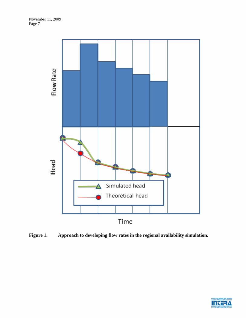
The calculated decline rate was used to determine a target head for each model cell on a yearly basis. This allowed for year-to-year adjustments of pumping to account for flow between cells and flow to or from boundaries. For each year, the model heads from the previous year were compared to the calculated target heads to determine the volume of water that could be removed from each cell during that year. These volumes were then combined with recharge for each cell to determine pumping rates. Figure 1 provides a hypothetical model cell pumping and head time series. In this example, the initial flow rate is calculated a priori to model simulation. However, the lower part of Figure 1 shows that the theoretical drawdown curve at the end of the first year is not achieved. This occurs because the flow rates are calculated assuming no flow from, or to, adjoining model cells. The new algorithm uses the theoretical drawdown curve to estimate the pumping rate for the next year. Through this approach, we successfully developed a method that follows the theoretical drawdown curve for each model cell closely and meets the design saturated thickness with the generation of no new inactive (dry) model cells. Results: The results determined to date include the regional groundwater availability and the available supplies for municipal and irrigation water user groups (WUGs) subject to drawdown criteria over 50 years and a pre-determined decline curve function. Results at this time are limited to the use of the existing GAM (Dutton, 2004). The drawdown criteria applied are consistent with the draft desired future conditions defined by GMA-1. This simulation differs significantly from the draft DFC/MAG simulation currently under review at the TWDB (GAM Run 09-001). Specifically, this simulation implements a consistent methodology for all regions, counties, and grid cells. Secondly, this simulation invokes the drawdown criteria at each model grid cell which implies groundwater management at the scale of one square mile. As a result, this simulation results in preservation of saturated thickness in all model grid blocks. This simulation does not increase inactive (dry) grid cells in the predictive time period. These modeling results do not take the place of the current TWDB draft DFC/MAG simulation (GAM Run 09-001) but rather augment understanding of the potential management of the resource under defined management criteria. Table 2 provides a summary of the annual regional groundwater availability by county as defined by the simulation described herein. Table 3 provides a summary of groundwater in place (storage) by county from the simulation described herein. This estimate of storage accounts for the variable specific yield implemented in the GAM. By dividing the 2060 groundwater in place by the 2010 groundwater in place and multiplying by 100 one should calculate the management criterion applied to that county minus round off. For the available supplies by WUG we analyzed the two largest WUGs, irrigation and municipal. To perform these calculations required definition of WUG zones for both categories within the model area. This required assignment of specific grid cells of the model with pumping associated with these two WUGs. A single cell could not be assigned multiple WUGs. Figure 2 provides the coverage of the irrigation zones used and Figure 3 provides the coverage of the municipal zones used. Each irrigation WUG zone was tracked by WUG type, county, river
November 11, 2009 Page 4
basin, and groundwater conservation district. Each municipal WUG zones was tracked by WUG type, county, river basin, and municipality. This approach resulted in 26 unique irrigation zones and 35 unique municipal zones. Table 4 provides the available irrigation supply by county and Table 5 provides the available municipal supply by county. One will note that in tables 4 and 5 the year 2011 has been added to the table in addition to the typical decadal reporting convention. The reason for this is that the initial pumping rate calculated for the year 2010 was typically an underestimate of the true rate required to attain the drawdown calculated for that one year time period. As a result, the algorithm developed corrected that rate in the next year of simulation to account for the communication between model cells. From that simulation year forward the flow rate was calculated specifically to attain a theoretical drawdown curve (see Figure 1). Generally after the year 2011 the flow rates were on a downward trend from 2012 through 2060. References: Dutton, A., 2004. Adjustments of Parameters to Improve the Calibration of the Og-n Model of the Ogallala Aquifer, Panhandle Water Planning Group, Prepared for Freese and Nichols, Inc. and the Panhandle Water Planning Group, June 2004.

November 11, 2009 Page 5
Table 2. Annual regional groundwater availability - AFY. County 2010 2020 2030 2040 2050 2060
Armstrong 48,916 40,834 36,089 31,978 28,462 25,383 Carson 198,232 178,545 160,493 144,656 129,882 116,336 Dallam 290,088 253,072 225,124 198,739 173,986 151,305 Donley 90,450 81,347 76,005 69,672 63,613 58,017 Gray 186,939 157,029 143,819 130,646 117,614 105,634 Hansford 279,085 258,780 238,529 217,640 195,835 174,892 Hartley 413,782 361,195 314,995 273,474 236,815 204,661 Hemphill 82,951 44,654 44,129 43,784 43,673 43,579 Hutchinson 153,829 129,548 119,798 108,985 98,239 87,979 Lipscomb 260,989 253,488 247,761 234,999 219,735 203,198 Moore 172,388 164,319 142,529 122,138 103,539 86,974 Ochiltree 257,903 236,618 215,489 195,506 176,566 159,017 Oldham 5,288 6,434 6,090 5,571 5,079 4,658 Potter 38,084 29,224 26,093 23,205 20,684 18,459 Randall 19,730 18,411 16,419 14,589 12,974 11,531 Roberts 375,334 339,518 322,909 301,420 277,509 251,933 Sherman 316,971 298,567 262,820 229,557 198,809 169,672 Wheeler 120,205 114,819 112,163 106,500 99,802 92,993 Sum 3,311,163 2,966,401 2,711,253 2,453,060 2,202,815 1,966,221
Table 3. Groundwater in place – AFY. County 2010 2020 2030 2040 2050 2060
Armstrong 3,393,836 2,980,888 2,614,958 2,292,115 2,007,702 1,757,463 Carson 14,523,374 12,748,607 11,166,494 9,751,901 8,489,527 7,367,135 Dallam 15,651,329 13,171,909 11,022,071 9,172,190 7,596,070 6,270,784 Donley 5,822,805 5,121,980 4,498,266 3,944,520 3,453,986 3,021,052 Gray 13,000,446 11,420,486 10,008,063 8,744,601 7,618,601 6,621,642 Hansford 20,769,174 18,218,902 15,883,250 13,768,737 11,879,677 10,213,135 Hartley 23,097,231 19,495,348 16,428,918 13,820,010 11,603,668 9,725,660 Hemphill 15,407,023 14,834,800 14,206,672 13,569,550 12,947,908 12,352,238 Hutchinson 10,542,798 9,248,736 8,078,744 7,025,960 6,087,234 5,257,916 Lipscomb 18,394,426 16,186,671 14,214,079 12,448,522 10,873,857 9,477,201 Moore 9,608,708 8,053,014 6,694,926 5,528,205 4,540,089 3,714,338 Ochiltree 19,066,318 16,739,260 14,648,686 12,768,510 11,083,298 9,580,902 Oldham 238,603 210,149 184,496 161,908 141,974 124,384 Potter 2,632,774 2,311,941 2,026,885 1,774,128 1,550,482 1,353,520 Randall 1,455,665 1,283,475 1,131,174 996,195 876,866 771,861 Roberts 26,852,172 23,590,451 20,655,707 18,018,243 15,657,191 13,557,937 Sherman 18,035,001 15,203,063 12,766,854 10,667,622 8,860,604 7,320,539 Wheeler 7,340,143 6,468,071 5,684,345 4,987,318 4,369,708 3,824,747 Sum 225,831,824 197,287,750 171,914,589 149,440,235 129,638,441 112,312,455

November 11, 2009 Page 6
Table 4. Available irrigation supplies by county (AFY). County 2010 2011 2020 2030 2040 2050 2060
Armstrong 4,863 6,639 5,767 5,051 4,477 3,962 3,511 Carson 99,376 109,908 101,110 92,086 83,796 75,773 67,954 Dallam 122,148 151,907 135,104 118,797 103,857 90,356 77,787 Donley 28,483 32,927 30,629 28,611 26,626 24,638 22,617 Gray 39,434 46,544 43,347 40,598 37,676 34,463 31,290 Hansford 91,195 117,316 114,936 109,261 101,068 90,839 80,500 Hartley 102,548 113,191 101,126 89,569 78,674 68,550 59,098 Hemphill 1,983 2,222 2,492 2,843 3,000 2,997 3,032 Hutchinson 27,517 27,621 27,921 27,126 25,605 23,581 21,394 Lipscomb 27,284 32,719 34,005 33,214 31,947 30,360 28,479 Moore 65,363 80,586 72,212 64,505 56,716 48,993 41,407 Ochiltree 57,568 72,556 67,470 63,162 58,444 53,619 48,921 Potter 1,788 3,131 2,469 1,929 1,555 1,290 1,065 Randall 4,104 6,390 4,857 4,356 3,918 3,495 3,080 Roberts 21,838 30,043 27,084 24,314 21,889 19,460 17,005 Sherman 121,224 147,808 131,122 114,716 99,927 86,586 74,048 Wheeler 10,429 12,558 12,818 12,440 11,961 11,309 10,537
Table 5. Available municipal supplies by county (AFY). County 2010 2011 2020 2030 2040 2050 2060
Armstrong 443 663 591 528 471 420 374 Carson 9,252 18,294 15,707 14,025 12,481 11,090 9,957 Dallam 1,841 2,068 2,321 2,483 2,477 2,357 2,182 Donley 255 248 239 214 194 176 161 Gray 2,040 2,361 1,562 1,152 768 624 541 Hansford 2,768 2,842 1,678 1,399 1,121 1,018 1,004 Hartley 2,066 3,033 2,550 2,045 1,606 1,231 965 Hemphill 238 377 354 356 372 386 399 Hutchinson 1,326 4,443 3,655 3,130 2,693 2,316 1,989 Lipscomb 2,710 3,277 3,749 4,056 4,125 4,047 3,885 Moore 2,253 2,898 2,155 1,693 1,306 1,007 737 Ochiltree 2,494 3,625 3,634 3,604 3,611 3,478 3,238 Potter 3,478 2,576 2,759 2,787 2,660 2,457 2,261 Randall 1,819 4,174 2,748 2,173 1,775 1,498 1,274 Roberts 16,531 31,742 29,155 27,733 26,200 24,283 22,274 Sherman 1,591 1,894 1,835 1,680 1,460 1,249 1,085 Wheeler 2,304 2,579 2,476 2,287 2,025 1,725 1,444
November 11, 2009 Page 7
Figure 1. Approach to developing flow rates in the regional availability simulation.

November 11, 2009 Page 8
Amarillo
Pampa
Dumas
Dalhart
Perryton
Cactus
Miami
Clarendon
Stinnett
Claude
Stratford
Panhandle
Fritch
Texhoma
Texline
Wheeler
Spearman
Sunray
White Deer
Follett
McLean
Higgins
Canadian
Booker
Channing
Gruver
Hedley
Groom
Borger
Mobeetie
Howardwick
Lefors
Skellytown
Darrouzett
Morse
Sanford
Lake TanglewoodLake Tanglewood
U60
I40
U54
U87
S15
S70
U8 3
U287
S152
S20
7
S33
S30
5
U38
5
S136
S102
I40 B
I27
S354
S213
S335
S203
S51
S273
S27
3
U287
U87
S70
U83
S273
I40S20
7S20
7
S70
S15
S20
7
S152
U385
DALLAM
HALL
OLDHAMGRAY
HARTLEY
DEAF SMITH
MOORE
POTTER
DONLEY
CARSON
CASTROPARMERBRISCOE
RANDALL
SWISHER
ROBERTS
WHEELER
SHERMAN
HEMPHILL
LIPSCOMBHANSFORD
OCHILTREE
ARMSTRONG
HUTCHINSON
CHILDRESS
COLLINGSWORTH
LAMB HALE FLOYDBAILEY MOTLEY COTTLE
HARDEMA
FOARD
−0 10 20
Miles
Irrigation Zones
IRR-ARMSTRONG-PGCD-RedRB
IRR-CARSON-PGCD-CanadianRB
IRR-CARSON-PGCD-RedRB
IRR-DALLAM-NPGCD-CanadianRB
IRR-DALLAM-noGCD-CanadianRB
IRR-DONLEY-PGCD-RedRB
IRR-GRAY-PGCD-CanadianRB
IRR-GRAY-PGCD-RedRB
IRR-HANSFORD-NPGCD-CanadianRB
IRR-HARTLEY-NPGCD-CanadianRB
IRR-HEMPHILL-HemphillGCD-CanadianRB
IRR-HUTCHINSON-NPGCD-CanadianRB
IRR-HUTCHINSON-noGCD-CanadianRB
IRR-LIPSCOMB-NPGCD-CanadianRB
IRR-MOORE-NPGCD-CanadianRB
IRR-OCHILTREE-NPGCD-CanadianRB
IRR-POTTER-HighPlainsGCD-RedRB
IRR-POTTER-PGCD-CanadianRB
IRR-POTTER-PGCD-RedRB
IRR-RANDALL-HighPlainsGCD-RedRB
IRR-RANDALL-noGCD-RedRB
IRR-ROBERTS-PGCD-CanadianRB
IRR-ROBERTS-PGCD-RedRB
IRR-SHERMAN-NPGCD-CanadianRB
IRR-WHEELER-PGCD-RedRB
IRR-HEMPHILL-HemphillGCD-REDRB
Irrigation Zones
Figure 2. Irrigation zones for available supplies calculations.

November 11, 2009 Page 9
DALLAM
HALL
OLDHAM
GRAY
HARTLEY
DEAF SMITH
MOORE
POTTER
DONLEY
CARSON
CASTROPARMERBRISCOE
RANDALL
SWISHER
ROBERTS
WHEELER
SHERMAN
HEMPHILL
LIPSCOMB
HANSFORD
OCHILTREE
ARMSTRONG
HUTCHINSON
CHILDRESS
COLLINGSWORTH
Amarillo
Pampa
Dumas
Dalhart
Perryton
Cactus
Miami
Clarendon
Stinnett
Claude
Stratford
Panhandle
Fritch
Texhoma
Texline
Wheeler
Spearman
Sunray
White Deer
Follett
McLean
Higgins
Canadian
Booker
Channing
Gruver
Hedley
Groom
Borger
Mobeetie
Howardwick
Lefors
Skellytown
Darrouzett
Morse
Sanford
Lake Tanglewood
U60
I40
U54
U87
S15
S70
U8 3
U287
S152
S207
S33
S30
5
U38
5
S136
S102
I40 B
I27
S354
S23
S213
S33
5
S51
S273
S17
1
S27
3
U287
U87
S70
U83
S136
S273
I40
S20
7S
2 07
S70
S15
S20
7
S152
U87
U385
−0 10 20
Miles
Municipal Zones
CRMWA
Borger TCW Supply
Fritch
Hi Texas Water Co.
Dumas
City of Amarillo
Memphis
Shamrock
Figure 3. Municipal zones for available supplies calculations.
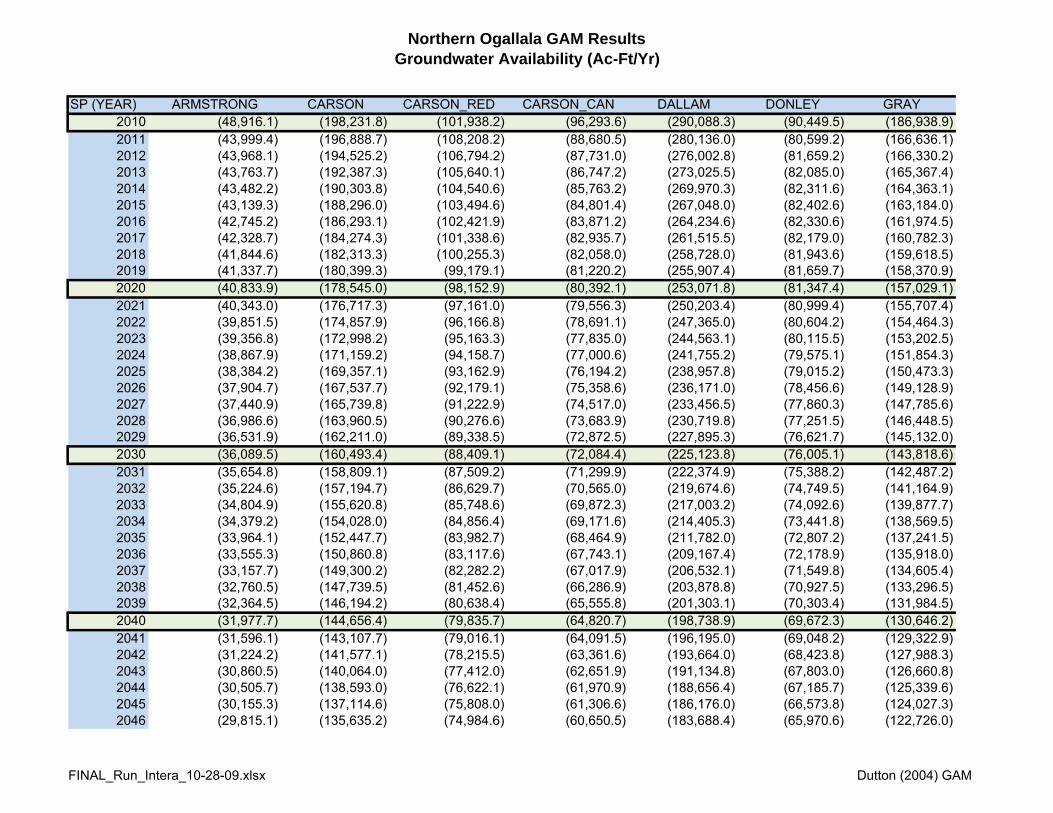
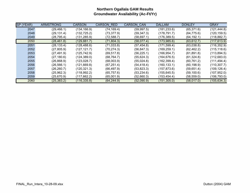
Northern Ogallala GAM ResultsGroundwater Availability (Ac-Ft/Yr)
SP (YEAR) ARMSTRONG CARSON CARSON_RED CARSON_CAN DALLAM DONLEY GRAY2010 (48,916.1) (198,231.8) (101,938.2) (96,293.6) (290,088.3) (90,449.5) (186,938.9) 2011 (43,999.4) (196,888.7) (108,208.2) (88,680.5) (280,136.0) (80,599.2) (166,636.1) 2012 (43,968.1) (194,525.2) (106,794.2) (87,731.0) (276,002.8) (81,659.2) (166,330.2) 2013 (43,763.7) (192,387.3) (105,640.1) (86,747.2) (273,025.5) (82,085.0) (165,367.4) 2014 (43,482.2) (190,303.8) (104,540.6) (85,763.2) (269,970.3) (82,311.6) (164,363.1) 2015 (43,139.3) (188,296.0) (103,494.6) (84,801.4) (267,048.0) (82,402.6) (163,184.0) 2016 (42,745.2) (186,293.1) (102,421.9) (83,871.2) (264,234.6) (82,330.6) (161,974.5) 2017 (42,328.7) (184,274.3) (101,338.6) (82,935.7) (261,515.5) (82,179.0) (160,782.3) 2018 (41,844.6) (182,313.3) (100,255.3) (82,058.0) (258,728.0) (81,943.6) (159,618.5) 2019 (41,337.7) (180,399.3) (99,179.1) (81,220.2) (255,907.4) (81,659.7) (158,370.9) 2020 (40,833.9) (178,545.0) (98,152.9) (80,392.1) (253,071.8) (81,347.4) (157,029.1) 2021 (40,343.0) (176,717.3) (97,161.0) (79,556.3) (250,203.4) (80,999.4) (155,707.4) 2022 (39,851.5) (174,857.9) (96,166.8) (78,691.1) (247,365.0) (80,604.2) (154,464.3) 2023 (39,356.8) (172,998.2) (95,163.3) (77,835.0) (244,563.1) (80,115.5) (153,202.5) 2024 (38,867.9) (171,159.2) (94,158.7) (77,000.6) (241,755.2) (79,575.1) (151,854.3) 2025 (38,384.2) (169,357.1) (93,162.9) (76,194.2) (238,957.8) (79,015.2) (150,473.3) 2026 (37,904.7) (167,537.7) (92,179.1) (75,358.6) (236,171.0) (78,456.6) (149,128.9) 2027 (37,440.9) (165,739.8) (91,222.9) (74,517.0) (233,456.5) (77,860.3) (147,785.6) 2028 (36,986.6) (163,960.5) (90,276.6) (73,683.9) (230,719.8) (77,251.5) (146,448.5) 2029 (36,531.9) (162,211.0) (89,338.5) (72,872.5) (227,895.3) (76,621.7) (145,132.0) 2030 (36,089.5) (160,493.4) (88,409.1) (72,084.4) (225,123.8) (76,005.1) (143,818.6) 2031 (35,654.8) (158,809.1) (87,509.2) (71,299.9) (222,374.9) (75,388.2) (142,487.2) 2032 (35,224.6) (157,194.7) (86,629.7) (70,565.0) (219,674.6) (74,749.5) (141,164.9) 2033 (34,804.9) (155,620.8) (85,748.6) (69,872.3) (217,003.2) (74,092.6) (139,877.7) 2034 (34,379.2) (154,028.0) (84,856.4) (69,171.6) (214,405.3) (73,441.8) (138,569.5) 2035 (33,964.1) (152,447.7) (83,982.7) (68,464.9) (211,782.0) (72,807.2) (137,241.5) 2036 (33,555.3) (150,860.8) (83,117.6) (67,743.1) (209,167.4) (72,178.9) (135,918.0) 2037 (33,157.7) (149,300.2) (82,282.2) (67,017.9) (206,532.1) (71,549.8) (134,605.4) 2038 (32,760.5) (147,739.5) (81,452.6) (66,286.9) (203,878.8) (70,927.5) (133,296.5) 2039 (32,364.5) (146,194.2) (80,638.4) (65,555.8) (201,303.1) (70,303.4) (131,984.5) 2040 (31,977.7) (144,656.4) (79,835.7) (64,820.7) (198,738.9) (69,672.3) (130,646.2) 2041 (31,596.1) (143,107.7) (79,016.1) (64,091.5) (196,195.0) (69,048.2) (129,322.9) 2042 (31,224.2) (141,577.1) (78,215.5) (63,361.6) (193,664.0) (68,423.8) (127,988.3) 2043 (30,860.5) (140,064.0) (77,412.0) (62,651.9) (191,134.8) (67,803.0) (126,660.8) 2044 (30,505.7) (138,593.0) (76,622.1) (61,970.9) (188,656.4) (67,185.7) (125,339.6) 2045 (30,155.3) (137,114.6) (75,808.0) (61,306.6) (186,176.0) (66,573.8) (124,027.3) 2046 (29,815.1) (135,635.2) (74,984.6) (60,650.5) (183,688.4) (65,970.6) (122,726.0)
FINAL_Run_Intera_10-28-09.xlsx Dutton (2004) GAM
Northern Ogallala GAM ResultsGroundwater Availability (Ac-Ft/Yr)
SP (YEAR) ARMSTRONG CARSON CARSON_RED CARSON_CAN DALLAM DONLEY GRAY2047 (29,466.1) (134,166.9) (74,169.4) (59,997.5) (181,233.6) (65,371.6) (121,444.8) 2048 (29,131.4) (132,725.2) (73,377.9) (59,347.3) (178,791.7) (64,775.6) (120,159.5) 2049 (28,795.4) (131,285.9) (72,588.7) (58,697.1) (176,389.5) (64,192.1) (118,882.7) 2050 (28,461.8) (129,881.7) (71,804.3) (58,077.4) (173,985.6) (63,612.7) (117,613.9) 2051 (28,133.4) (128,488.6) (71,033.8) (57,454.8) (171,599.4) (63,038.8) (116,352.9) 2052 (27,805.9) (127,121.7) (70,274.3) (56,847.3) (169,259.1) (62,462.2) (115,118.6) 2053 (27,491.9) (125,742.9) (69,517.8) (56,225.1) (166,954.7) (61,891.8) (113,894.5) 2054 (27,180.6) (124,389.0) (68,764.7) (55,624.3) (164,676.5) (61,324.8) (112,683.0) 2055 (26,868.9) (123,028.7) (68,003.9) (55,024.8) (162,399.4) (60,761.2) (111,494.4) 2056 (26,566.1) (121,669.8) (67,251.4) (54,418.4) (160,133.1) (60,198.9) (110,307.7) 2057 (26,260.7) (120,321.3) (66,497.9) (53,823.3) (157,873.6) (59,651.4) (109,126.4) 2058 (25,962.3) (118,992.2) (65,757.6) (53,234.6) (155,645.5) (59,100.6) (107,952.0) 2059 (25,670.9) (117,662.2) (65,001.9) (52,660.3) (153,454.4) (58,559.0) (106,793.0) 2060 (25,383.2) (116,335.8) (64,244.9) (52,090.9) (151,305.0) (58,017.0) (105,634.3)
FINAL_Run_Intera_10-28-09.xlsx Dutton (2004) GAM
Northern Ogallala GAM ResultsGroundwater Availability (Ac-Ft/Yr)
SP (YEAR)2010201120122013201420152016201720182019202020212022202320242025202620272028202920302031203220332034203520362037203820392040204120422043204420452046
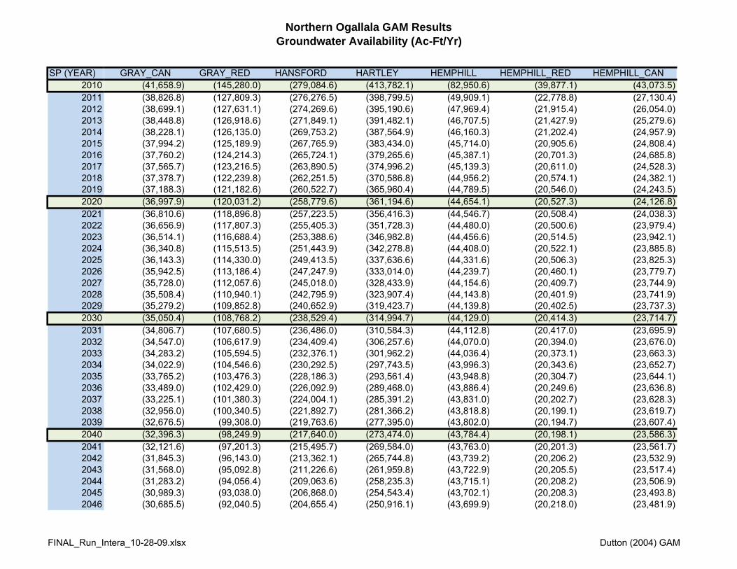
GRAY_CAN GRAY_RED HANSFORD HARTLEY HEMPHILL HEMPHILL_RED HEMPHILL_CAN(41,658.9) (145,280.0) (279,084.6) (413,782.1) (82,950.6) (39,877.1) (43,073.5) (38,826.8) (127,809.3) (276,276.5) (398,799.5) (49,909.1) (22,778.8) (27,130.4) (38,699.1) (127,631.1) (274,269.6) (395,190.6) (47,969.4) (21,915.4) (26,054.0) (38,448.8) (126,918.6) (271,849.1) (391,482.1) (46,707.5) (21,427.9) (25,279.6) (38,228.1) (126,135.0) (269,753.2) (387,564.9) (46,160.3) (21,202.4) (24,957.9) (37,994.2) (125,189.9) (267,765.9) (383,434.0) (45,714.0) (20,905.6) (24,808.4) (37,760.2) (124,214.3) (265,724.1) (379,265.6) (45,387.1) (20,701.3) (24,685.8) (37,565.7) (123,216.5) (263,890.5) (374,996.2) (45,139.3) (20,611.0) (24,528.3) (37,378.7) (122,239.8) (262,251.5) (370,586.8) (44,956.2) (20,574.1) (24,382.1) (37,188.3) (121,182.6) (260,522.7) (365,960.4) (44,789.5) (20,546.0) (24,243.5) (36,997.9) (120,031.2) (258,779.6) (361,194.6) (44,654.1) (20,527.3) (24,126.8) (36,810.6) (118,896.8) (257,223.5) (356,416.3) (44,546.7) (20,508.4) (24,038.3) (36,656.9) (117,807.3) (255,405.3) (351,728.3) (44,480.0) (20,500.6) (23,979.4) (36,514.1) (116,688.4) (253,388.6) (346,982.8) (44,456.6) (20,514.5) (23,942.1) (36,340.8) (115,513.5) (251,443.9) (342,278.8) (44,408.0) (20,522.1) (23,885.8) (36,143.3) (114,330.0) (249,413.5) (337,636.6) (44,331.6) (20,506.3) (23,825.3) (35,942.5) (113,186.4) (247,247.9) (333,014.0) (44,239.7) (20,460.1) (23,779.7) (35,728.0) (112,057.6) (245,018.0) (328,433.9) (44,154.6) (20,409.7) (23,744.9) (35,508.4) (110,940.1) (242,795.9) (323,907.4) (44,143.8) (20,401.9) (23,741.9) (35,279.2) (109,852.8) (240,652.9) (319,423.7) (44,139.8) (20,402.5) (23,737.3) (35,050.4) (108,768.2) (238,529.4) (314,994.7) (44,129.0) (20,414.3) (23,714.7) (34,806.7) (107,680.5) (236,486.0) (310,584.3) (44,112.8) (20,417.0) (23,695.9) (34,547.0) (106,617.9) (234,409.4) (306,257.6) (44,070.0) (20,394.0) (23,676.0) (34,283.2) (105,594.5) (232,376.1) (301,962.2) (44,036.4) (20,373.1) (23,663.3) (34,022.9) (104,546.6) (230,292.5) (297,743.5) (43,996.3) (20,343.6) (23,652.7) (33,765.2) (103,476.3) (228,186.3) (293,561.4) (43,948.8) (20,304.7) (23,644.1) (33,489.0) (102,429.0) (226,092.9) (289,468.0) (43,886.4) (20,249.6) (23,636.8) (33,225.1) (101,380.3) (224,004.1) (285,391.2) (43,831.0) (20,202.7) (23,628.3) (32,956.0) (100,340.5) (221,892.7) (281,366.2) (43,818.8) (20,199.1) (23,619.7) (32,676.5) (99,308.0) (219,763.6) (277,395.0) (43,802.0) (20,194.7) (23,607.4) (32,396.3) (98,249.9) (217,640.0) (273,474.0) (43,784.4) (20,198.1) (23,586.3) (32,121.6) (97,201.3) (215,495.7) (269,584.0) (43,763.0) (20,201.3) (23,561.7) (31,845.3) (96,143.0) (213,362.1) (265,744.8) (43,739.2) (20,206.2) (23,532.9) (31,568.0) (95,092.8) (211,226.6) (261,959.8) (43,722.9) (20,205.5) (23,517.4) (31,283.2) (94,056.4) (209,063.6) (258,235.3) (43,715.1) (20,208.2) (23,506.9) (30,989.3) (93,038.0) (206,868.0) (254,543.4) (43,702.1) (20,208.3) (23,493.8) (30,685.5) (92,040.5) (204,655.4) (250,916.1) (43,699.9) (20,218.0) (23,481.9)
FINAL_Run_Intera_10-28-09.xlsx Dutton (2004) GAM

Northern Ogallala GAM ResultsGroundwater Availability (Ac-Ft/Yr)
SP (YEAR)20472048204920502051205220532054205520562057205820592060
GRAY_CAN GRAY_RED HANSFORD HARTLEY HEMPHILL HEMPHILL_RED HEMPHILL_CAN(30,379.8) (91,065.0) (202,445.2) (247,319.9) (43,697.6) (20,230.8) (23,466.8) (30,075.7) (90,083.7) (200,231.4) (243,783.9) (43,696.4) (20,245.1) (23,451.3) (29,767.1) (89,115.5) (198,029.4) (240,274.6) (43,688.6) (20,256.1) (23,432.6) (29,456.6) (88,157.4) (195,835.4) (236,815.0) (43,672.7) (20,255.8) (23,416.9) (29,146.7) (87,206.3) (193,685.6) (233,390.9) (43,654.7) (20,248.0) (23,406.7) (28,844.6) (86,274.0) (191,553.5) (230,014.3) (43,641.1) (20,241.2) (23,399.9) (28,541.0) (85,353.4) (189,423.7) (226,713.3) (43,642.8) (20,236.1) (23,406.8) (28,239.6) (84,443.4) (187,325.9) (223,446.8) (43,636.4) (20,227.5) (23,408.8) (27,949.5) (83,544.9) (185,277.8) (220,222.7) (43,631.2) (20,214.9) (23,416.3) (27,654.0) (82,653.8) (183,193.2) (217,030.5) (43,620.8) (20,198.3) (23,422.5) (27,355.4) (81,771.1) (181,103.5) (213,880.8) (43,610.3) (20,176.0) (23,434.3) (27,060.7) (80,891.3) (179,004.5) (210,780.2) (43,600.5) (20,158.3) (23,442.1) (26,767.4) (80,025.5) (176,933.6) (207,696.0) (43,591.3) (20,142.6) (23,448.8) (26,479.9) (79,154.3) (174,892.3) (204,660.9) (43,578.7) (20,132.2) (23,446.5)
FINAL_Run_Intera_10-28-09.xlsx Dutton (2004) GAM

Northern Ogallala GAM ResultsGroundwater Availability (Ac-Ft/Yr)
SP (YEAR)2010201120122013201420152016201720182019202020212022202320242025202620272028202920302031203220332034203520362037203820392040204120422043204420452046
HUTCHINSON LIPSCOMB MOORE OCHILTREE OLDHAM POTTER POTTER_CAN(153,829.2) (260,988.7) (172,388.3) (257,903.5) (5,288.2) (38,083.6) (30,284.0) (135,941.4) (245,529.7) (182,771.3) (257,080.2) (4,857.1) (31,477.3) (24,932.1) (135,189.0) (247,846.3) (180,386.7) (254,476.8) (5,218.6) (31,484.5) (25,022.3) (134,432.7) (249,409.0) (178,488.3) (252,283.5) (5,470.4) (31,241.0) (24,885.8) (133,866.8) (250,695.2) (176,627.0) (250,023.9) (5,704.7) (30,999.9) (24,747.0) (133,288.2) (251,634.8) (174,706.9) (247,787.1) (5,911.4) (30,752.5) (24,600.4) (132,671.6) (252,350.4) (172,720.2) (245,491.8) (6,105.5) (30,460.9) (24,406.8) (132,016.1) (252,841.1) (170,776.4) (243,191.4) (6,242.0) (30,155.3) (24,198.2) (131,308.6) (253,185.4) (168,707.6) (240,999.0) (6,349.5) (29,846.7) (23,983.4) (130,473.1) (253,405.6) (166,524.0) (238,835.9) (6,430.0) (29,530.6) (23,759.6) (129,548.1) (253,487.6) (164,318.8) (236,618.5) (6,433.6) (29,223.7) (23,543.3) (128,611.6) (253,372.2) (162,126.0) (234,405.1) (6,421.6) (28,920.5) (23,328.5) (127,645.8) (253,108.0) (159,904.7) (232,222.3) (6,404.7) (28,616.2) (23,111.5) (126,753.2) (252,733.9) (157,662.5) (230,106.9) (6,385.9) (28,292.5) (22,872.4) (125,897.1) (252,238.1) (155,458.0) (228,009.1) (6,363.9) (27,964.6) (22,627.5) (124,992.7) (251,685.9) (153,279.6) (225,962.2) (6,327.0) (27,635.8) (22,380.9) (124,003.7) (251,061.0) (151,077.4) (223,891.8) (6,280.4) (27,319.4) (22,142.0) (122,988.5) (250,398.6) (148,910.7) (221,781.5) (6,235.0) (27,001.8) (21,903.4) (121,942.6) (249,666.6) (146,789.2) (219,691.7) (6,187.9) (26,690.3) (21,667.9) (120,893.7) (248,764.7) (144,660.0) (217,588.8) (6,139.6) (26,394.0) (21,445.6) (119,797.9) (247,761.1) (142,528.7) (215,489.0) (6,090.0) (26,093.4) (21,215.8) (118,692.7) (246,680.6) (140,357.2) (213,466.6) (6,039.3) (25,780.5) (20,976.1) (117,584.6) (245,531.7) (138,245.1) (211,483.5) (5,988.1) (25,473.1) (20,738.1) (116,497.9) (244,331.3) (136,178.5) (209,438.7) (5,936.7) (25,170.1) (20,502.9) (115,431.3) (243,073.4) (134,131.2) (207,402.5) (5,884.9) (24,873.0) (20,272.6) (114,372.0) (241,811.5) (132,102.5) (205,377.6) (5,831.5) (24,576.7) (20,041.9) (113,301.0) (240,514.0) (130,065.1) (203,350.1) (5,778.7) (24,296.3) (19,827.0) (112,214.5) (239,166.2) (128,014.7) (201,337.1) (5,725.7) (24,011.9) (19,607.8) (111,136.3) (237,810.5) (126,004.0) (199,361.8) (5,672.2) (23,738.7) (19,397.1) (110,060.6) (236,418.4) (124,064.6) (197,438.7) (5,622.1) (23,469.4) (19,190.2) (108,985.5) (234,998.7) (122,137.5) (195,505.7) (5,571.0) (23,204.6) (18,985.7) (107,915.0) (233,567.7) (120,219.4) (193,563.3) (5,519.7) (22,936.7) (18,779.2) (106,838.2) (232,107.2) (118,281.6) (191,633.7) (5,469.3) (22,675.8) (18,576.6) (105,758.8) (230,614.2) (116,377.3) (189,696.4) (5,418.5) (22,420.3) (18,376.5) (104,691.8) (229,104.1) (114,485.3) (187,767.6) (5,368.1) (22,161.3) (18,175.9) (103,608.6) (227,566.3) (112,597.4) (185,857.1) (5,318.3) (21,905.2) (17,973.1) (102,501.3) (226,034.4) (110,809.4) (183,951.7) (5,268.7) (21,659.6) (17,779.7)
FINAL_Run_Intera_10-28-09.xlsx Dutton (2004) GAM
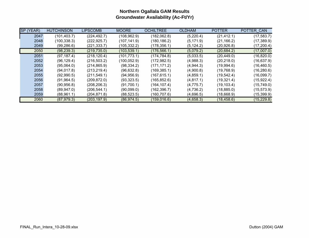
Northern Ogallala GAM ResultsGroundwater Availability (Ac-Ft/Yr)
SP (YEAR)20472048204920502051205220532054205520562057205820592060
HUTCHINSON LIPSCOMB MOORE OCHILTREE OLDHAM POTTER POTTER_CAN(101,403.7) (224,492.7) (108,962.9) (182,062.8) (5,220.4) (21,412.1) (17,583.7) (100,338.3) (222,925.7) (107,141.9) (180,186.2) (5,171.9) (21,166.2) (17,389.9) (99,286.6) (221,333.7) (105,332.2) (178,356.1) (5,124.2) (20,926.8) (17,200.4) (98,239.3) (219,735.0) (103,539.1) (176,566.1) (5,079.2) (20,684.2) (17,007.0) (97,187.4) (218,120.4) (101,773.1) (174,784.8) (5,033.5) (20,449.0) (16,820.0) (96,129.4) (216,503.2) (100,052.9) (172,982.5) (4,988.3) (20,218.0) (16,637.9) (95,064.0) (214,865.9) (98,334.2) (171,171.2) (4,944.3) (19,994.6) (16,460.5) (94,017.8) (213,219.4) (96,632.8) (169,385.1) (4,900.8) (19,768.9) (16,280.6) (92,990.5) (211,549.1) (94,956.9) (167,615.1) (4,859.1) (19,542.4) (16,099.7) (91,964.5) (209,872.0) (93,323.5) (165,852.6) (4,817.1) (19,321.4) (15,922.4) (90,956.8) (208,206.3) (91,700.1) (164,107.4) (4,775.7) (19,103.4) (15,749.0) (89,947.0) (206,544.1) (90,099.0) (162,396.7) (4,736.2) (18,885.0) (15,573.9) (88,961.1) (204,871.8) (88,523.5) (160,707.6) (4,696.5) (18,668.9) (15,399.9) (87,979.3) (203,197.9) (86,974.5) (159,016.6) (4,658.3) (18,458.6) (15,229.8)
FINAL_Run_Intera_10-28-09.xlsx Dutton (2004) GAM

Northern Ogallala GAM ResultsGroundwater Availability (Ac-Ft/Yr)
SP (YEAR)2010201120122013201420152016201720182019202020212022202320242025202620272028202920302031203220332034203520362037203820392040204120422043204420452046
POTTER_RED RANDALL ROBERTS ROBERTS_CAN ROBERTS_RED SHERMAN WHEELER(7,799.7) (19,729.9) (375,334.2) (361,045.1) (14,289.1) (316,970.6) (120,205.2) (6,545.2) (22,578.8) (345,056.7) (330,363.6) (14,693.1) (331,069.3) (101,705.6) (6,462.2) (21,500.4) (344,853.7) (329,698.6) (15,155.1) (326,912.4) (105,614.5) (6,355.2) (20,926.1) (344,692.0) (329,109.9) (15,582.1) (323,893.1) (108,234.9) (6,252.9) (20,422.7) (344,526.9) (328,593.9) (15,933.0) (320,414.5) (110,356.2) (6,152.1) (19,984.6) (344,187.3) (327,976.8) (16,210.5) (316,816.4) (111,947.6) (6,054.1) (19,579.6) (343,805.7) (327,363.3) (16,442.4) (313,160.2) (113,035.0) (5,957.0) (19,229.1) (343,264.6) (326,627.0) (16,637.6) (309,519.1) (113,784.5) (5,863.3) (18,918.2) (342,180.8) (325,407.4) (16,773.4) (305,909.3) (114,309.0) (5,771.1) (18,650.3) (340,922.2) (324,043.5) (16,878.6) (302,301.8) (114,665.4) (5,680.4) (18,411.1) (339,517.7) (322,555.7) (16,962.0) (298,567.5) (114,819.0) (5,592.0) (18,186.0) (338,086.7) (321,061.6) (17,025.2) (294,893.7) (114,816.2) (5,504.7) (17,970.4) (336,630.9) (319,557.5) (17,073.4) (291,269.6) (114,675.5) (5,420.1) (17,757.7) (334,944.7) (317,851.6) (17,093.1) (287,632.1) (114,461.6) (5,337.1) (17,564.4) (333,236.5) (316,148.9) (17,087.5) (284,041.3) (114,218.9) (5,255.0) (17,369.6) (331,547.8) (314,477.2) (17,070.6) (280,477.7) (113,951.9) (5,177.4) (17,179.5) (329,929.1) (312,885.4) (17,043.7) (276,951.9) (113,655.4) (5,098.4) (16,982.8) (328,285.6) (311,277.3) (17,008.3) (273,388.0) (113,318.8) (5,022.4) (16,789.9) (326,589.3) (309,624.6) (16,964.7) (269,865.6) (112,939.7) (4,948.4) (16,598.7) (324,822.7) (307,910.1) (16,912.6) (266,333.5) (112,547.9) (4,877.6) (16,418.6) (322,908.8) (306,054.1) (16,854.8) (262,819.5) (112,162.6) (4,804.4) (16,225.2) (320,887.5) (304,096.7) (16,790.7) (259,369.9) (111,724.9) (4,735.0) (16,038.8) (318,768.2) (302,047.9) (16,720.3) (255,945.2) (111,225.1) (4,667.2) (15,850.0) (316,722.5) (300,083.5) (16,639.0) (252,544.3) (110,694.3) (4,600.4) (15,661.9) (314,666.3) (298,115.6) (16,550.7) (249,142.1) (110,145.1) (4,534.7) (15,474.2) (312,491.7) (296,037.6) (16,454.1) (245,741.4) (109,573.6) (4,469.3) (15,291.1) (310,258.0) (293,907.1) (16,350.9) (242,408.3) (108,997.5) (4,404.1) (15,112.0) (308,004.0) (291,760.7) (16,243.3) (239,154.8) (108,396.1) (4,341.6) (14,935.5) (305,778.4) (289,648.6) (16,129.7) (235,939.8) (107,778.6) (4,279.2) (14,762.1) (303,612.3) (287,597.8) (16,014.5) (232,753.2) (107,142.9) (4,218.9) (14,589.1) (301,420.3) (285,524.7) (15,895.6) (229,557.3) (106,500.1) (4,157.5) (14,419.2) (299,134.9) (283,358.8) (15,776.1) (226,421.8) (105,854.1) (4,099.2) (14,248.7) (296,813.8) (281,159.4) (15,654.4) (223,312.3) (105,210.7) (4,043.8) (14,083.1) (294,429.6) (278,898.2) (15,531.4) (220,232.7) (104,554.7) (3,985.4) (13,923.0) (292,043.0) (276,635.3) (15,407.8) (217,136.4) (103,888.5) (3,932.2) (13,761.5) (289,706.5) (274,423.2) (15,283.3) (214,052.5) (103,212.9) (3,879.9) (13,603.5) (287,350.5) (272,191.5) (15,159.0) (210,965.5) (102,532.8)
FINAL_Run_Intera_10-28-09.xlsx Dutton (2004) GAM

Northern Ogallala GAM ResultsGroundwater Availability (Ac-Ft/Yr)
SP (YEAR)20472048204920502051205220532054205520562057205820592060
POTTER_RED RANDALL ROBERTS ROBERTS_CAN ROBERTS_RED SHERMAN WHEELER(3,828.4) (13,443.9) (284,979.8) (269,935.5) (15,044.3) (207,904.3) (101,861.5) (3,776.3) (13,288.1) (282,520.8) (267,594.9) (14,925.9) (204,872.0) (101,171.9) (3,726.3) (13,129.2) (280,017.0) (265,211.2) (14,805.8) (201,825.9) (100,485.0) (3,677.1) (12,973.9) (277,508.6) (262,824.7) (14,683.9) (198,809.3) (99,801.5) (3,629.0) (12,821.4) (275,003.2) (260,442.3) (14,560.9) (195,801.9) (99,124.2) (3,580.2) (12,664.8) (272,468.6) (258,031.7) (14,436.9) (192,823.1) (98,444.3) (3,534.2) (12,518.1) (269,917.6) (255,603.6) (14,314.0) (189,860.7) (97,759.2) (3,488.3) (12,369.9) (267,377.5) (253,187.4) (14,190.1) (186,896.7) (97,081.7) (3,442.6) (12,225.2) (264,840.8) (250,774.5) (14,066.3) (183,935.6) (96,396.8) (3,399.0) (12,085.6) (262,302.4) (248,360.0) (13,942.4) (181,011.6) (95,713.1) (3,354.4) (11,945.4) (259,733.5) (245,910.2) (13,823.3) (178,121.4) (95,027.5) (3,311.1) (11,806.3) (257,132.7) (243,424.0) (13,708.7) (175,261.9) (94,346.9) (3,269.1) (11,666.8) (254,541.3) (240,949.9) (13,591.4) (172,452.7) (93,671.0) (3,228.8) (11,530.9) (251,932.7) (238,459.1) (13,473.6) (169,671.7) (92,993.3)
FINAL_Run_Intera_10-28-09.xlsx Dutton (2004) GAM
Intera Incorporated 1812 Centre Creek Drive, Suite 300 Austin, Texas 78754 Telephone: 512 425 2000 Fax: 512 425 2099
M E M O R A N D U M
To: Simone Kiel, Freese and Nichols, Inc. From: Van Kelley, INTERA Dennis Fryar, INTERA Date: July 29, 2010
RE: Baseline Simulation Results Using the Dutton (2004) GAM with Updated Pumping Demands
The revised GAM (INTERA, 2010) documented in Appendix F of this plan was not completed in time to be completely incorporated into the Initially Prepared Plan. As a result, simulations to support the planning process were made using the 2004 Dutton GAM (Dutton, 2004) updated to include updated historical (1950-2008) pumping and an updated predictive demand distribution (2009-2060).
A baseline simulation was performed to determine the capability of the aquifer to meet projected demands through 2060 with current infrastructure. Table D-1 summarizes the groundwater in storage in the PWPA for the baseline simulation across the predictive simulation period from 2010 through 2060.
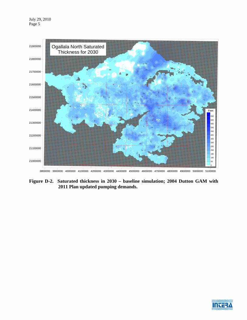
Figure D-1 shows the saturated thickness of the aquifer simulated by the GAM in the year 2010. One can see that in 2010 most of the Northern Ogallala in Texas is saturated with the largest number of inactive cells (representing dry aquifer conditions and white in the figure) in Dallam County. Figures D-2 and D-3 provide similar saturated thickness plots for the years 2030 and 2060, respectively. By 2060 one can see that significant portions of the aquifer in Dallam, Hartley, Moore and Sherman counties have become inactive. The baseline analysis shows that with projected pumping there will be significant areas of the aquifer with significant depletion. Many of these areas occur in heavily irrigated areas. As areas of the model region become over-pumped, the model cells become inactive which represents dry aquifer conditions. In reality, there will likely be a thin saturated thickness in these portions of the aquifer in the future because pumping efficiency will decrease to such a degree that desaturation of the aquifer will be uneconomical. When a model cell becomes inactive, the pumping that is assigned to that cell as a demand cannot be satisfied and these wells are effectively shut off.
Table D-2 provides a summary of the pumping demand requested of the model on a county basis by decade from 2010 through 2060. Table D-3 provides a summary of the pumping volume actually pumped from each county by decade from 2010 through 2060. In the period between 2010 and 2060 the annual average demand for the Ogallala is 1,303,482 acre-ft/year in Region A. However, the model predicts that users will only be able to pump an average annual amount
July 29, 2010 Page 2
of 969,212 acre-ft/year for the planning period. By the year 2060, the model predicts that pumping will be reduced by approximately 44.9 percent from the pumping demand.
References: Dutton, A., 2004. Adjustments of Parameters to Improve the Calibration of the Og-n Model of the Ogallala Aquifer, Panhandle Water Planning Group, Prepared for Freese and Nichols, Inc. and the Panhandle Water Planning Group, June 2004.
INTERA, 2010. Northern Ogallala Update to Support 2011 State Water Plan, Submitted to the Panhandle Area Water Planning Group, February 2010, Included as Appendix F of this Regional Water Plan for the Panhandle Water Planning Area.
Table D-1 Groundwater in storage (acre-ft), baseline simulation(1). County 2010 2020 2030 2040 2050 2060
Armstrong 3,422,773 3,386,035 3,350,603 3,316,695 3,285,329 3,257,389 Carson 14,071,052 13,519,741 13,005,845 12,514,858 12,085,200 11,713,447 Collingsworth 85,793 85,696 85,600 85,511 85,430 85,361 Dallam 14,420,421 12,504,805 10,931,542 9,783,757 8,991,767 8,462,420 Donley 5,733,509 5,496,388 5,295,354 5,121,490 4,977,372 4,866,096 Gray 13,126,321 12,852,731 12,601,443 12,363,648 12,150,490 11,961,188 Hansford 20,409,655 19,271,486 18,237,164 17,258,378 16,386,542 15,633,384 Hartley 21,747,772 19,377,289 17,700,362 16,616,557 15,941,982 15,484,458 Hemphill 15,473,075 15,429,244 15,391,305 15,359,662 15,334,260 15,314,243 Hutchinson 10,553,132 9,932,670 9,380,780 8,888,808 8,478,132 8,130,914 Lipscomb 18,458,532 18,264,312 18,094,708 17,943,872 17,818,846 17,722,298 Moore 9,073,330 7,800,781 6,654,934 5,647,404 4,918,946 4,434,168 Ochiltree 19,104,748 18,628,312 18,189,073 17,767,415 17,381,757 17,042,149 Oldham 348,291 347,997 347,638 347,183 346,613 345,929 Potter 2,679,448 2,541,100 2,441,898 2,354,113 2,278,140 2,230,359 Randall 1,644,728 1,639,999 1,631,057 1,622,772 1,616,472 1,609,374 Roberts 27,078,546 26,266,991 25,543,758 24,997,372 24,543,081 24,192,427 Sherman 17,294,485 15,442,185 13,754,762 12,197,899 10,880,317 9,830,743 Wheeler 7,415,354 7,351,351 7,298,190 7,252,283 7,215,583 7,188,348 Sum 222,140,963 210,139,113 199,936,014 191,439,679 184,716,258 179,504,693
(1) Simulations results using the 2004 Dutton GAM with 2011 Plan updated pumping demands

July 29, 2010 Page 3
Table D-2 Groundwater pumping demand (acre-ft) – baseline simulation(1). County 2010 2020 2030 2040 2050 2060
Armstrong 3,410 3,295 3,209 3,073 2,817 2,557 Carson 68,003 58,348 60,281 57,497 47,771 45,958 Collingsworth 0 0 0 0 0 0 Dallam 282,335 274,929 266,771 252,853 224,580 196,260 Donley 32,353 30,019 29,096 27,563 24,518 21,468 Gray 29,428 26,222 26,632 25,863 24,477 22,385 Hansford 131,074 115,976 112,902 107,564 96,482 85,421 Hartley 296,286 285,034 277,076 263,478 235,664 207,936 Hemphill 5,396 5,285 4,956 4,384 3,836 3,346 Hutchinson 65,137 63,632 63,754 62,948 59,852 57,541 Lipscomb 30,583 28,210 27,291 25,733 22,893 20,078 Moore 150,074 139,282 137,125 132,845 121,040 109,251 Ochiltree 61,419 53,254 51,910 49,459 44,554 39,689 Oldham 1 1 1 1 1 0 Potter 13,344 12,569 11,859 10,970 10,129 9,384 Randall 7,865 7,631 7,915 8,144 8,131 8,033 Roberts 57,377 76,004 75,690 75,152 74,369 67,190 Sherman 228,557 208,975 203,141 191,877 172,757 152,394 Wheeler 10,021 8,727 8,368 7,733 6,794 5,896 Sum 1,472,661 1,397,393 1,367,975 1,307,136 1,180,663 1,054,789
(1) Simulations results using the 2004 Dutton GAM with 2011 Plan updated pumping demands
Table D-3 Actual groundwater pumping (acre-ft) – baseline simulation(1). County 2010 2020 2030 2040 2050 2060
Armstrong 2,575 2,530 2,468 2,370 2,193 2,011 Carson 68,003 58,348 60,281 57,497 47,771 45,365 Collingsworth 0 0 0 0 0 0 Dallam 227,098 189,908 150,979 112,347 80,176 59,718 Donley 32,353 27,249 25,838 23,160 20,260 17,250 Gray 26,622 23,866 23,418 22,179 19,772 17,741 Hansford 131,074 115,975 112,901 106,527 95,027 83,831 Hartley 274,329 213,607 146,551 96,754 64,542 50,626 Hemphill 5,396 5,285 4,956 4,384 3,836 3,346 Hutchinson 62,505 53,783 49,785 41,502 35,226 28,659 Lipscomb 30,583 28,210 27,290 25,733 22,893 20,078 Moore 145,288 127,205 114,947 95,252 65,509 41,390 Ochiltree 60,950 52,854 51,522 49,092 44,228 39,403 Oldham 1 1 1 1 1 0 Potter 13,344 9,201 8,787 8,252 6,504 4,528 Randall 6,941 6,821 6,945 6,756 6,604 6,642 Roberts 57,377 76,003 60,594 52,882 43,685 32,734 Sherman 228,556 206,130 194,352 176,793 147,465 121,598 Wheeler 10,021 8,727 8,368 7,733 6,794 5,896 Sum 1,383,012 1,205,703 1,049,983 889,212 712,486 580,817
(1) Simulations results using the 2004 Dutton GAM with 2011 Plan updated pumping demands

July 29, 2010 Page 4
3800000 3900000 4000000 4100000 4200000 4300000 4400000 4500000 4600000 4700000 4800000 4900000 5000000 5100000
21000000
21100000
21200000
21300000
21400000
21500000
21600000
21700000
21800000
21900000
0
50
100
150
200
250
300
350
400
450
500
550
600
650
Feet
Ogallala North SaturatedThickness for 2010
Figure D-1. Saturated thickness in 2010 – baseline simulation; 2004 Dutton GAM with
2011 Plan updated pumping demands.
July 29, 2010 Page 5
3800000 3900000 4000000 4100000 4200000 4300000 4400000 4500000 4600000 4700000 4800000 4900000 5000000 5100000
21000000
21100000
21200000
21300000
21400000
21500000
21600000
21700000
21800000
21900000
0
50
100
150
200
250
300
350
400
450
500
550
600
650
Feet
Ogallala North SaturatedThickness for 2030
Figure D-2. Saturated thickness in 2030 – baseline simulation; 2004 Dutton GAM with
2011 Plan updated pumping demands.

July 29, 2010 Page 6
3800000 3900000 4000000 4100000 4200000 4300000 4400000 4500000 4600000 4700000 4800000 4900000 5000000 5100000
21000000
21100000
21200000
21300000
21400000
21500000
21600000
21700000
21800000
21900000
0
50
100
150
200
250
300
350
400
450
500
550
600
650
Feet
Ogallala North SaturatedThickness for 2060
Figure D-3. Saturated thickness in 2060 – baseline simulation; 2004 Dutton GAM with
2011 Plan updated pumping demands.
GAM run 04-22
by Roberto Anaya, Scott Hamlin, and Shirley Wade Texas Water Development Board Groundwater Availability Modeling Section (512) 936-2415 March 4, 2005
REQUESTOR: Mr. Stefan Schuster with Freese and Nichols, Inc. on behalf of the Panhandle Regional Water Planning Group DESCRIPTION OF REQUEST: Determine the groundwater volume in storage for the Blaine aquifer in Childress, Collingsworth, Hall, and Wheeler counties and for the Seymour aquifer in Childress, Collingsworth, and Hall counties for the years 2000 to 2060 on a decadal basis using the Groundwater Availability Model (GAM) for the Seymour aquifer (Ewing, and others, 2004). METHODS: To address the request, we ran the GAM for the Seymour aquifer using average annual recharge for the period through 2060 and predictive pumpage based on new demands that the Panhandle Regional Water Planning Group plans to include in their 2006 regional water plan. We saved water-level values for the Blaine and the Seymour aquifers for the end of each decade and imported them into ArcView. Some water levels (less than 10 percent of the active cells) exceeded the land surface. We adjusted these water levels to land surface and calculated the saturated thicknesses of the aquifers. We then multiplied the saturated thickness by the appropriate area and specific yield to calculate groundwater volumes. PARAMETERS AND ASSUMPTIONS:
• See Ewing and others (2004) for assumptions and limitations of the GAM. Root mean squared error for this model ranges from 9.7 feet to 27.5 feet for the Seymour aquifer and is 26.4 feet for the Blaine aquifer (Ewing and others, 2004). This error will have more of an effect on model results where the aquifer is thin.
• We used a specific yield of 0.05 for the Blaine aquifer and 0.15 for the Seymour aquifer.
• Recharge represents average conditions for the predictive period.
1

RESULTS: The volume of groundwater from the Seymour and Blaine aquifers in the counties are listed in Table 1. Note that the GAM run may include less pumpage than initially assigned because, according to the GAM, the Seymour aquifer cannot support the pumpage and begins to go dry. In the GAM, once a part of the model goes dry, it stays dry, and the pumping is “shut off.” This can result in water levels rising in nearby areas once the pumping in the area is stopped (Table 1). This also results in less pumping in the model because the pumping has been stopped in these areas. In reality, the aquifer will probably not go dry because pumping will become uneconomical before the aquifer goes dry in any particular area. However, the GAM is suggesting that these areas may experience water supply problems sometime in the next 50 years. REFERENCES: Ewing, J. E., Jones, T. L., Pickens, J. F., Chastain-Howley, A., Dean, K. E., Spear, and A.
A., 2004, Groundwater availability model for the Seymour aquifer: final report prepared for the Texas Water Development Board by INTERA Inc., 432 p.
2

Table 1. Volume of groundwater in the Blaine and Seymour aquifers for counties in the Panhandle Regional Water Planning Area
based on the GAM for the Seymour aquifer.
Blaine aquifer Groundwater volumes in acre-feet County 2000 2010 2020 2030 2040 2050 2060
Childress 4,900,000 5,000,000 5,000,000 5,000,000 5,000,000 5,000,000 5,000,000Collingsworth 10,000,000 10,000,000 10,000,000 10,000,000 10,000,000 10,000,000 10,000,000Hall 800,000 800,000 800,000 800,000 800,000 800,000 800,000Wheeler 2,600,000 2,600,000 2,500,000 2,500,000 2,500,000 2,500,000 2,500,000
Seymour aquifer Groundwater volumes in acre-feet
County 2000 2010 2020 2030 2040 2050 2060Childress 130,000 130,000 130,000 140,000 140,000 140,000 140,000Collingsworth 520,000 480,000 460,000 450,000 450,000 460,000 470,000Hall 210,000 200,000 180,000 180,000 180,000 190,000 190,000
- values are rounded to two significant figures
3

GAM run 05-11 by Richard Smith, PG
Texas Water Development Board Groundwater Availability Modeling Section (512) 936-0877 March 4, 2005
REQUESTOR: Mr. Stefan Schuster with Freese and Nichols, Inc. on behalf of the Panhandle Regional Water Planning Group DESCRIPTION OF REQUEST: Mr. Schuster requested that we run the Groundwater Availability Model (GAM) for the southern part of the Ogallala aquifer for the period 2000 to 2050 for Randall and Oldham counties and (1) compute groundwater volumes for the same counties and (2) estimate groundwater volumes for 2060. He wanted this information for 2000, 2010, 2020, 2030, 2040, 2050, and 2060. METHODS: We used the GAM for the southern part of the Ogallala aquifer (Blandford and others, 2003) with average recharge and the 2000 to 2050 predictive scenario. We calculated saturated thickness by subtracting the bottom of the Ogallala aquifer, as included in the GAM, from the GAM calculated water levels. We then used ArcView to generate total volumes for each county based on the saturated thickness for each decade. On a cell-by-cell basis in the GAM, we multiplied the saturated thickness by the area of the cell and by a specific yield of 0.15. We used trend line projections, as calculated in Excel, to estimate aquifer volumes for 2060. In addition, we adjusted the partial values listed in Table 1 of GAM run 05-10 (Smith and Mace, 2005) for Oldham and Randall counties to reflect the full aquifer volumes for these counties and included the results in this report. PARAMETERS AND ASSUMPTIONS:
• See Blandford and others (2003) for assumptions and limitations of the GAM. Root mean squared error for this model is 44 ft. This error will have more of an effect on model results where the aquifer is thin.
• Recharge represents average conditions for the predictive period. • Assumed a uniform specific yield of 0.15 across aquifer. • Assumed the trend line analysis represents a reasonable projection based on 2000
to 2050 volumes.
1

RESULTS: Table 1 shows the estimated aquifer volumes for the parts of Oldham and Randall counties that were modeled in the GAM of the southern part of the Ogallala aquifer. Note that the GAM run may include less pumpage than initially assigned because, according to the GAM, the aquifer cannot support the pumpage and begins to go dry in Randall County. In the GAM, once a part of the model goes dry, it stays dry, and the pumping is “shut off.” This can result in water levels rising in nearby areas once the pumping in the area is stopped (Figure 1). This also results in less pumping in the model because the pumping has been stopped in these areas. In reality, the aquifer will probably not go dry because pumping will become uneconomical before the aquifer goes dry in any particular area. However, the GAM is suggesting that these areas may experience water supply problems sometime in the next 50 years. The polynomial trend line and linear analysis to project the aquifer volume for 2060 for Randall and Oldham counties had a 98 percent R-squared value and a 90 percent R-squared value, respectively (see Figures 1 and 2). Table 2 shows the adjusted groundwater volumes to reflect all of Oldham and Randall counties. The projected volumes are consistently higher than the 1.25% analysis from GAM run 04-13 (Smith, 2004). See GAM Run 05-10 (Smith and Mace, 2005) for an analysis of what these numbers mean. REFERENCES: Blandford, T. N., Blazer, D. J., Calhoun, K. C., Dutton, A. R., Naing, T., Reedy, R. C.,
and Scanlon, B. R., 2003, Groundwater Availability of the Southern Ogallala Aquifer in Texas and New Mexico; Numerical Simulations Through 2050: final report prepared for the Texas Water Development Board.
Smith, R., 2004, GAM Run 04-13: Texas Water Development Board, 7 p. Smith, R., 2005, GAM Run 05-09: Texas Water Development Board, 14 p. Smith, R. and Mace, R., 2005, GAM Run 05-10: Texas Water Development Board, 4 p.
2

Table 1. Estimates of groundwater volumes for the portions of Oldham and Randall counties located in the GAM of the southern part of the Ogallala aquifer.
County GAM 2000 (acre-feet)
GAM 2010 (acre-feet)
GAM 2020 (acre-feet)
GAM 2030 (acre-feet)
GAM 2040 (acre-feet)
GAM 2050 (acre-feet)
*GAM 2060 (acre-feet)
Oldham 2,220,000 2,120,000 2,100,000 2,070,000 2,050,000 2,050,000 1,990,000Randall 4,840,000 4,370,000 4,100,000 4,040,000 4,140,000 4,220,000 4,620,000
- Values are rounded to three significant figures. * 2060 is not based on the GAM.
Table 2. Update to Table 1 in GAM run 05-10 for Oldham and Randall counties reflecting the combination of aquifer volumes from the northern and southern parts of the GAMs of the Ogallala aquifer.
1.25% GAM 1.25% GAM 1.25% GAM 1.25% GAM 1.25% GAM 2000 2000 2010 2010 2020 2020 2030 2030 2040 2040 County (acre-feet) (acre-feet) (acre-feet) (acre-feet) (acre-feet) (acre-feet) (acre-feet) (acre-feet) (acre-feet) (acre-feet) Oldham* 2,580,000 2,660,000 2,310,000 2,560,000 2,080,000 2,530,000 1,870,000 2,490,000 1,690,000 2,470,000 Randall* 6,230,000 6,400,000 5,730,000 5,820,000 5,290,000 5,460,000 4,900,000 5,320,000 4,560,000 5,360,000 1.25% GAM 1.25% GAM 2050 2050 2060 2060 County (acre-feet) (acre-feet) (acre-feet) (acre-feet) Oldham* 1,530,000 2,460,000 1,390,000 2,400,000** Randall* 4,250,000 5,390,000 3,990,000 5,750,000** - Values are rounded to three significant figures. * Additional information on the method and assumptions used to calculate the 1.25% reduction can be found in GAM run 04-13 (Smith, 2004) and the method and assumptions used to estimate the portion of the counties in the northern portion of the Ogallala aquifer GAM can be found in GAM run 05-09 (Smith, 2005). ** 2060 is not based on the GAM.
3

Randall County Trendline Analysis
4,000,000
4,100,000
4,200,000
4,300,000
4,400,000
4,500,000
4,600,000
4,700,000
4,800,000
4,900,000
5,000,000
2000 2010 2020 2030 2040 2050 2060
Year
Estim
ated
gro
undw
ater
vol
umes
(acr
e-fe
et)
Randall County Poly. (Randall County)
Figure 1. Polynomial best fit trend analysis for groundwater volume in Randall County (Equation is y =76,429x2 – 644,286x + 5,380,000; R2 = 0.9811).
4
Oldham County Trendline Analysis
1,900,000
1,950,000
2,000,000
2,050,000
2,100,000
2,150,000
2,200,000
2,250,000
2,300,000
2000 2010 2020 2030 2040 2050 2060
Year
Estim
ated
gro
undw
ater
vol
umes
(acr
e-fe
et)
Oldham County Linear (Oldham County)
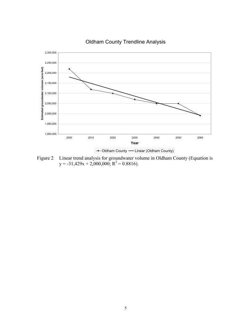
Figure 2 Linear trend analysis for groundwater volume in Oldham County (Equation is y = -31,429x + 2,000,000; R2 = 0.8816).
5

1
GAM run 05-16
by Richard Smith, P.G. Texas Water Development Board Groundwater Availability Modeling Section (512) 936-0877 June 12, 2005
REQUESTOR: Mr. Stefan Schuster with Freese and Nichols, Inc. on behalf of the Panhandle Regional Water Planning Group DESCRIPTION OF REQUEST: Mr. Schuster requested that we run the Groundwater Availability Model (GAM) for the southern part of the Ogallala aquifer for the period 1950 to 2060 and provide maps of saturated thicknesses for 1950, 1960, 1970, 1980, 1990, 2000, 2010, 2020, 2030, 2040, 2050, and 2060 in Oldham, Potter, and Randall counties. METHODS: We used the Groundwater Availability Model (GAM) for the southern part of the Ogallala aquifer (Blandford and others, 2003). For the historical simulation (1950 to 1999), we used pumpage as included in the GAM. For the predictive simulation (2000 to 2060), we used the water demand projections for water user groups of the Llano Estacado Regional Water Planning Group, as approved by the Texas Water Development Board on September 17, 2003, for the period of record through 2060 (see GAM run 03-36). In GAM run 05-11, volumes in 2060 for Oldham and Randall counties were projected using polynomial trend line and linear analysis. This was done as a simplification and the resulting values are essentially the same as the GAM values for the same year using the pumpage from GAM run 03-36. Once we ran the GAM, we calculated saturated thickness by subtracting the bottom elevation of the Ogallala aquifer as included in the GAM from the GAM calculated water levels. We contoured the saturated thickness data on a cell-by-cell basis within PMWIN to create maps. PARAMETERS AND ASSUMPTIONS:
• See Blandford and others (2003) for assumptions and limitations of the GAM. Root mean squared error for this model is 34 feet. This error will have more of an effect on model results where the aquifer is thin.
• Recharge represents average conditions for the predictive period. • Assumed a uniform specific yield of 0.15 across the aquifer.
2
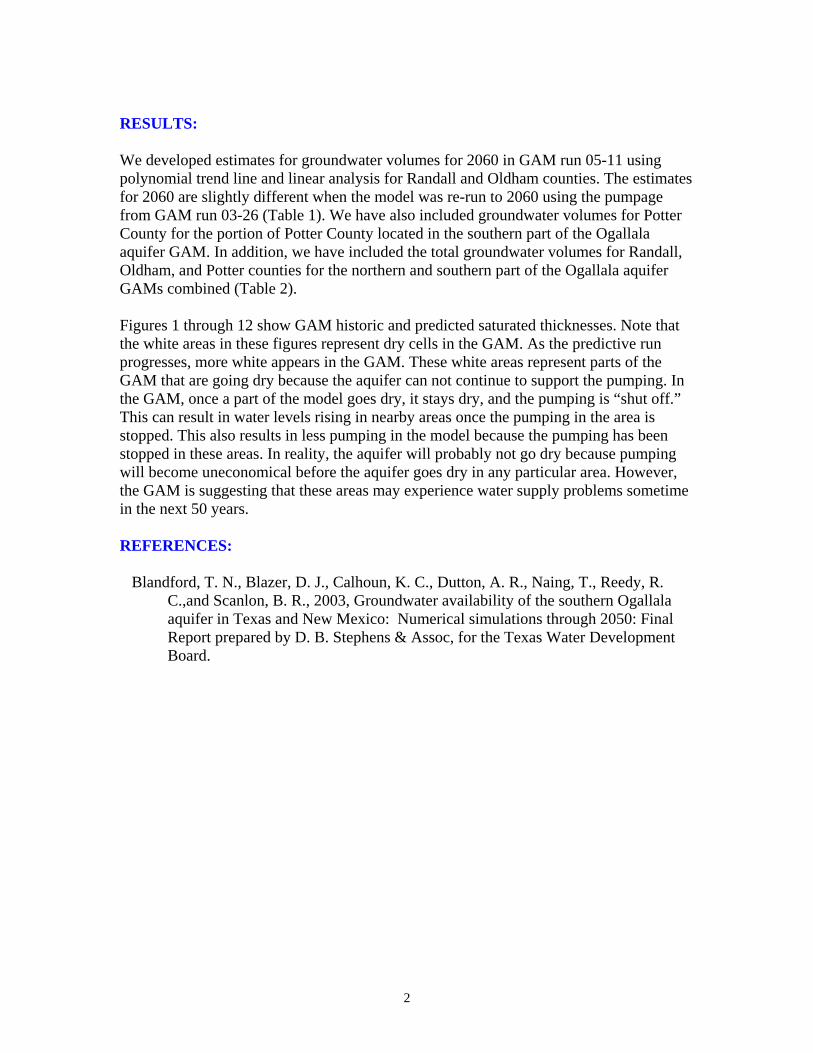
RESULTS: We developed estimates for groundwater volumes for 2060 in GAM run 05-11 using polynomial trend line and linear analysis for Randall and Oldham counties. The estimates for 2060 are slightly different when the model was re-run to 2060 using the pumpage from GAM run 03-26 (Table 1). We have also included groundwater volumes for Potter County for the portion of Potter County located in the southern part of the Ogallala aquifer GAM. In addition, we have included the total groundwater volumes for Randall, Oldham, and Potter counties for the northern and southern part of the Ogallala aquifer GAMs combined (Table 2). Figures 1 through 12 show GAM historic and predicted saturated thicknesses. Note that the white areas in these figures represent dry cells in the GAM. As the predictive run progresses, more white appears in the GAM. These white areas represent parts of the GAM that are going dry because the aquifer can not continue to support the pumping. In the GAM, once a part of the model goes dry, it stays dry, and the pumping is “shut off.” This can result in water levels rising in nearby areas once the pumping in the area is stopped. This also results in less pumping in the model because the pumping has been stopped in these areas. In reality, the aquifer will probably not go dry because pumping will become uneconomical before the aquifer goes dry in any particular area. However, the GAM is suggesting that these areas may experience water supply problems sometime in the next 50 years. REFERENCES:
Blandford, T. N., Blazer, D. J., Calhoun, K. C., Dutton, A. R., Naing, T., Reedy, R. C.,and Scanlon, B. R., 2003, Groundwater availability of the southern Ogallala aquifer in Texas and New Mexico: Numerical simulations through 2050: Final Report prepared by D. B. Stephens & Assoc, for the Texas Water Development Board.

3
Table 1. Estimates of groundwater volumes for the portions of Oldham, Randall, and Potter counties located in the GAM of the southern part of the Ogallala aquifer.
County GAM 2000 (acre-feet)
GAM 2010 (acre-feet)
GAM 2020 (acre-feet)
GAM 2030 (acre-feet)
GAM 2040 (acre-feet)
GAM 2050 (acre-feet)
GAM 2060 (acre-feet)
Oldham 2,220,000 2,120,00 0 2,100,00 0 2,070,000 2,050,000 2,050,000 2,040,000Randall 4,840,000 4,370,00 0 4,100,00 0 4,040,000 4,140,000 4,220,000 4,210,000Potter 294,000 241,00 0 213,00 0 204,000 203,000 202,000 200,000
- Values are rounded to three significant figures.
Table 2. Update to Table 1 in GAM run 05-10 for Oldham, Randall, and Potter counties reflecting the combination of aquifer volumes from the northern and southern parts of the GAMs of the Ogallala aquifer.
1.25% GAM 1.25% GAM 1.25% GAM 1.25% GAM 1.25% GAM 2000 2000 2010 2010 2020 2020 2030 2030 2040 2040 County (acre-feet) (acre-feet) (acre-feet) (acre-feet) (acre-feet) (acre-feet) (acre-feet) (acre-feet) (acre-feet) (acre-feet) Oldham* 2,580,000 2,660,000 2,310,000 2,560,000 2,080,000 2,530,000 1,870,000 2,490,000 1,690,000 2,470,000 Randall* 6,230,000 6,400,000 5,730,000 5,820,000 5,290,000 5,460,000 4,900,000 5,320,000 4,560,000 5,360,000 Potter 2,790,000 3,084,000 2,490,000 2,921,000 2,230,000 2,743,000 2,000,000 2,614,000 1,800,000 2,543,000 1.25% GAM 1.25% GAM 2050 2050 2060 2060 County (acre-feet) (acre-feet) (acre-feet) (acre-feet) Oldham* 1,530,000 2,460,000 1,390,000 2,450,000 Randall* 4,250,000 5,390,000 3,990,000 5,340,000 Potter 1,620,000 2,262,000 1,460,000 2,390,000 - Values are rounded to three significant figures. * Additional information on the method and assumptions used to calculate the 1.25% reduction can be found in GAM run 04-13 (Smith, 2004) and the method and assumptions used to estimate the portion of the counties in the northern portion of the Ogallala aquifer GAM can be found in GAM run 05-09 (Smith, 2005).

9
Figure 6: Simulated saturated thickness in feet of the Ogallala aquifer in Oldham, Potter, Deaf Smith, and Randall counties for 2000.
North is at the top of the map, and county boundaries are shown in yellow. Inactive cells are in dark gray, and dry cells are white.
15
Figure 12: Simulated saturated thickness in feet of the Ogallala aquifer in Oldham, Potter, Deaf Smith, and Randall counties for 2060.
North is at the top of the map, and county boundaries are shown in yellow. Inactive cells are in dark gray, and dry cells are white.
1
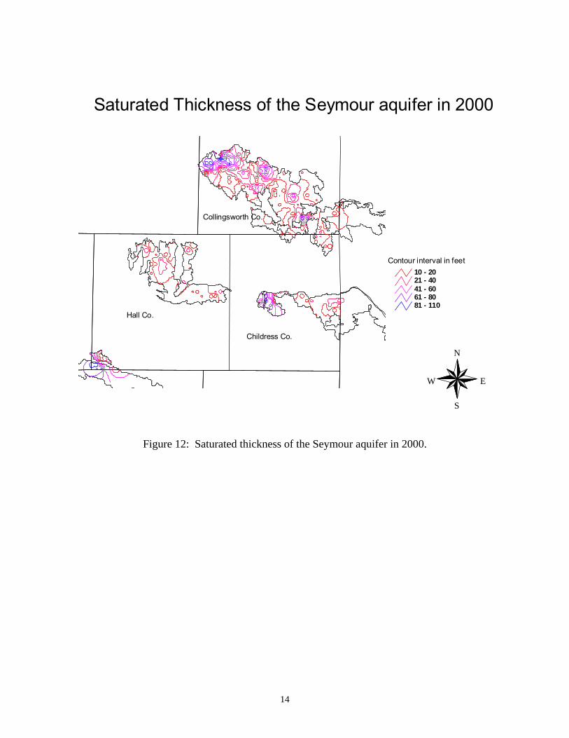
GAM run 05-17
by Richard Smith, P.G. Texas Water Development Board Groundwater Availability Modeling Section (512) 936-0877 May 16, 2005
REQUESTOR: Mr. Stefan Schuster with Freese and Nichols, Inc. on behalf of the Panhandle Regional Water Planning Group DESCRIPTION OF REQUEST: Mr. Schuster requested that we run the Groundwater Availability Model (GAM) for the Seymour and Blaine aquifers for the period 1975 to 2060 and provide maps of saturated thicknesses for 1980, 1990, 2000, 2010, 2020, 2030, 2040, 2050, and 2060 in Hall, Childress, Collingsworth and Wheeler counties for the Blaine aquifer and Hall, Childress, and Collingsworth counties for the Seymour aquifer. METHODS: We used the Groundwater Availability Model (GAM) for the Seymour aquifer (Ewing, and others, 2004). For the historical simulation (1975 to 1999), we used pumpage as included in the GAM with average annual recharge. We ran the GAM for the Seymour aquifer using average annual recharge for the period through 2060 and predictive pumpage based on new demands that the Panhandle Regional Water Planning Group plans to include in their 2006 regional water plan. Once we ran the GAM, we calculated saturated thickness by subtracting the bottom elevation of the Seymour aquifer as included in the GAM from the GAM calculated water levels. If the calculated water level exceeded the elevation of the top of the Seymour, the water level was changed to match the elevation value and then the difference between the top and bottom elevations was considered the saturated thickness. We used the same procedure to calculate the saturated thickness of the Blaine in Hall, Childress, Collingsworth, and Wheeler counties. We imported the saturated thickness data on a cell-by-cell basis into Surfer8© for the Blaine aquifer and we contoured the information to create maps. We calculated and contoured the saturated thickness of the Seymour aquifer in Hall, Childress, and Collingsworth counties using ArcView. PARAMETERS AND ASSUMPTIONS:
• See Ewing and others (2004) for assumptions and limitations of the GAM. • Root mean squared error for this model ranges from 9.7 feet to 27.5 feet for the
Seymour aquifer and is 26.4 feet for the Blaine aquifer (Ewing and others, 2004). This error will have more of an effect on model results where the aquifer is thin
2
• Recharge represents average conditions for the predictive and historical period. RESULTS: Figures 1 through 9 show GAM historic and predicted saturated thicknesses for the Blaine aquifer. Figures 10 through 18 show GAM historic and predicted saturated thicknesses for the Seymour aquifer. REFERENCES: Ewing, J. E., Jones, T. L., Pickens, J. F., Chastain-Howley, A., Dean, K. E., Spear, and A.
A., 2004, Groundwater availability model for the Seymour aquifer: final report prepared for the Texas Water Development Board by INTERA Inc., 432 p.

5
4800000 4850000 4900000
20900000
21000000
21100000
Figure 3: Saturated Thickness in feet of the Blaine aquifer in Childress, Collingsworth Hall and Wheeler counties in 2000. North is at the top of the figure and the maps units are in feet.
Childress Co..
Collingsworth Co.
Wheeler Co.
140
180
200
240
280
300
340
380
400
440
480
Hall Co.

11
Figure 9: Saturated Thickness in feet of the Blaine aquifer in Childress, Collingsworth Hall and Wheeler counties in 2060. North is at the top of the figure and the maps units are in feet.
Childress Co..
Collingsworth Co.
Wheeler Co.
Hall Co.
4800000 4850000 4900000
20900000
21000000
21100000
140
180
200
240
280
300
340
380
400
440
480
14
N
EW
S
10 - 2021 - 4041 - 6061 - 8081 - 110
Contour interval in feet
Childress Co.
Hall Co.
Collingsworth Co.
Saturated Thickness of the Seymour aquifer in 2000
Figure 12: Saturated thickness of the Seymour aquifer in 2000.

20
N
EW
S
10 - 2021 - 4041 - 6061 - 8081 - 100
Saturated Thickness of the Seymour aquifer in 2060
Contour interval in feetChildress Co.
Collingsworth Co.
Hall Co.
Figure 18: Saturated thickness of the Seymour aquifer in 2060.


