HPCToolkit User’s Manual

John Mellor-CrummeyLaksono Adhianto, Mike Fagan, Mark Krentel, Nathan Tallent

Rice University

October 9, 2017

Contents

1 Introduction 1

2 HPCToolkit Overview 52.1 Asynchronous Sampling . . . . . . . . . . . . . . . . . . . . . . . . . . . . . 52.2 Call Path Profiling . . . . . . . . . . . . . . . . . . . . . . . . . . . . . . . . 62.3 Recovering Static Program Structure . . . . . . . . . . . . . . . . . . . . . . 72.4 Presenting Performance Measurements . . . . . . . . . . . . . . . . . . . . . 8

3 Quick Start 93.1 Guided Tour . . . . . . . . . . . . . . . . . . . . . . . . . . . . . . . . . . . 9

3.1.1 Compiling an Application . . . . . . . . . . . . . . . . . . . . . . . . 93.1.2 Measuring Application Performance . . . . . . . . . . . . . . . . . . 103.1.3 Recovering Program Structure . . . . . . . . . . . . . . . . . . . . . 113.1.4 Analyzing Measurements & Attributing them to Source Code . . . . 113.1.5 Presenting Performance Measurements for Interactive Analysis . . . 123.1.6 Effective Performance Analysis Techniques . . . . . . . . . . . . . . 12

3.2 Additional Guidance . . . . . . . . . . . . . . . . . . . . . . . . . . . . . . . 13

4 Effective Strategies for Analyzing Program Performance 144.1 Monitoring High-Latency Penalty Events . . . . . . . . . . . . . . . . . . . 144.2 Computing Derived Metrics . . . . . . . . . . . . . . . . . . . . . . . . . . . 144.3 Pinpointing and Quantifying Inefficiencies . . . . . . . . . . . . . . . . . . . 174.4 Pinpointing and Quantifying Scalability Bottlenecks . . . . . . . . . . . . . 19

4.4.1 Scalability Analysis Using Expectations . . . . . . . . . . . . . . . . 21

5 Running Applications with hpcrun and hpclink 255.1 Using hpcrun . . . . . . . . . . . . . . . . . . . . . . . . . . . . . . . . . . . 255.2 Using hpclink . . . . . . . . . . . . . . . . . . . . . . . . . . . . . . . . . . 265.3 Sample Sources . . . . . . . . . . . . . . . . . . . . . . . . . . . . . . . . . . 26

5.3.1 Linux perf events . . . . . . . . . . . . . . . . . . . . . . . . . . . . 265.3.2 PAPI . . . . . . . . . . . . . . . . . . . . . . . . . . . . . . . . . . . 295.3.3 Wallclock, Realtime and Cputime . . . . . . . . . . . . . . . . . . . . 305.3.4 IO . . . . . . . . . . . . . . . . . . . . . . . . . . . . . . . . . . . . . 315.3.5 Memleak . . . . . . . . . . . . . . . . . . . . . . . . . . . . . . . . . 32

5.4 Process Fraction . . . . . . . . . . . . . . . . . . . . . . . . . . . . . . . . . 33

i

5.5 Starting and Stopping Sampling . . . . . . . . . . . . . . . . . . . . . . . . 335.6 Environment Variables for hpcrun . . . . . . . . . . . . . . . . . . . . . . . 355.7 Platform-Specific Notes . . . . . . . . . . . . . . . . . . . . . . . . . . . . . 35

5.7.1 Cray XE6 and XK6 . . . . . . . . . . . . . . . . . . . . . . . . . . . 35

6 hpcviewer’s User Interface 376.1 Launching . . . . . . . . . . . . . . . . . . . . . . . . . . . . . . . . . . . . . 376.2 Views . . . . . . . . . . . . . . . . . . . . . . . . . . . . . . . . . . . . . . . 376.3 Panes . . . . . . . . . . . . . . . . . . . . . . . . . . . . . . . . . . . . . . . 39

6.3.1 Source pane . . . . . . . . . . . . . . . . . . . . . . . . . . . . . . . . 396.3.2 Navigation pane . . . . . . . . . . . . . . . . . . . . . . . . . . . . . 396.3.3 Metric pane . . . . . . . . . . . . . . . . . . . . . . . . . . . . . . . . 42

6.4 Understanding Metrics . . . . . . . . . . . . . . . . . . . . . . . . . . . . . . 426.4.1 How metrics are computed? . . . . . . . . . . . . . . . . . . . . . . . 436.4.2 Example . . . . . . . . . . . . . . . . . . . . . . . . . . . . . . . . . . 43

6.5 Derived Metrics . . . . . . . . . . . . . . . . . . . . . . . . . . . . . . . . . . 456.5.1 Formulae . . . . . . . . . . . . . . . . . . . . . . . . . . . . . . . . . 456.5.2 Examples . . . . . . . . . . . . . . . . . . . . . . . . . . . . . . . . . 456.5.3 Derived metric dialog box . . . . . . . . . . . . . . . . . . . . . . . . 45

6.6 Thread-level Metric Values . . . . . . . . . . . . . . . . . . . . . . . . . . . 476.6.1 Plotting graphs . . . . . . . . . . . . . . . . . . . . . . . . . . . . . . 476.6.2 Thread View . . . . . . . . . . . . . . . . . . . . . . . . . . . . . . . 48

6.7 Filtering Tree nodes . . . . . . . . . . . . . . . . . . . . . . . . . . . . . . . 496.8 For Convenience Sake . . . . . . . . . . . . . . . . . . . . . . . . . . . . . . 51

6.8.1 Editor pane . . . . . . . . . . . . . . . . . . . . . . . . . . . . . . . . 516.8.2 Metric pane . . . . . . . . . . . . . . . . . . . . . . . . . . . . . . . . 52

6.9 Menus . . . . . . . . . . . . . . . . . . . . . . . . . . . . . . . . . . . . . . . 536.9.1 File . . . . . . . . . . . . . . . . . . . . . . . . . . . . . . . . . . . . 536.9.2 Filter . . . . . . . . . . . . . . . . . . . . . . . . . . . . . . . . . . . 546.9.3 View . . . . . . . . . . . . . . . . . . . . . . . . . . . . . . . . . . . . 546.9.4 Window . . . . . . . . . . . . . . . . . . . . . . . . . . . . . . . . . . 546.9.5 Help . . . . . . . . . . . . . . . . . . . . . . . . . . . . . . . . . . . . 54

6.10 Limitations . . . . . . . . . . . . . . . . . . . . . . . . . . . . . . . . . . . . 54

7 hpctraceviewer’s User Interface 557.1 hpctraceviewer overview . . . . . . . . . . . . . . . . . . . . . . . . . . . . 557.2 Launching . . . . . . . . . . . . . . . . . . . . . . . . . . . . . . . . . . . . . 567.3 Views . . . . . . . . . . . . . . . . . . . . . . . . . . . . . . . . . . . . . . . 56

7.3.1 Trace view . . . . . . . . . . . . . . . . . . . . . . . . . . . . . . . . 587.3.2 Depth view . . . . . . . . . . . . . . . . . . . . . . . . . . . . . . . . 597.3.3 Summary view . . . . . . . . . . . . . . . . . . . . . . . . . . . . . . 597.3.4 Call path view . . . . . . . . . . . . . . . . . . . . . . . . . . . . . . 607.3.5 Mini map view . . . . . . . . . . . . . . . . . . . . . . . . . . . . . . 60

7.4 Menus . . . . . . . . . . . . . . . . . . . . . . . . . . . . . . . . . . . . . . . 607.5 Limitations . . . . . . . . . . . . . . . . . . . . . . . . . . . . . . . . . . . . 62

8 Monitoring MPI Applications 648.1 Introduction . . . . . . . . . . . . . . . . . . . . . . . . . . . . . . . . . . . . 648.2 Running and Analyzing MPI Programs . . . . . . . . . . . . . . . . . . . . 648.3 Building and Installing HPCToolkit . . . . . . . . . . . . . . . . . . . . . 66

9 Monitoring Statically Linked Applications 679.1 Linking with hpclink . . . . . . . . . . . . . . . . . . . . . . . . . . . . . . 679.2 Running a Statically Linked Binary . . . . . . . . . . . . . . . . . . . . . . . 689.3 Troubleshooting . . . . . . . . . . . . . . . . . . . . . . . . . . . . . . . . . . 68

10 FAQ and Troubleshooting 7010.1 How do I choose hpcrun sampling periods? . . . . . . . . . . . . . . . . . . 7010.2 hpcrun incurs high overhead! Why? . . . . . . . . . . . . . . . . . . . . . . 7010.3 Fail to run hpcviewer: executable launcher was unable to locate its compan-

ion shared library . . . . . . . . . . . . . . . . . . . . . . . . . . . . . . . . . 7110.4 When executing hpcviewer, it complains cannot create “Java Virtual Machine” 7110.5 hpcviewer fails to launch due to java.lang.NoSuchMethodError exception. . 7210.6 hpcviewer writes a long list of Java error messages to the terminal! . . . . 7210.7 hpcviewer attributes performance information only to functions and not to

source code loops and lines! Why? . . . . . . . . . . . . . . . . . . . . . . . 7210.8 hpcviewer hangs trying to open a large database! Why? . . . . . . . . . . . 7310.9 hpcviewer runs glacially slowly! Why? . . . . . . . . . . . . . . . . . . . . . 7310.10hpcviewer does not show my source code! Why? . . . . . . . . . . . . . . . 74

10.10.1 Follow ‘Best Practices’ . . . . . . . . . . . . . . . . . . . . . . . . . . 7410.10.2 Additional Background . . . . . . . . . . . . . . . . . . . . . . . . . 74

10.11hpcviewer’s reported line numbers do not exactly correspond to what I seein my source code! Why? . . . . . . . . . . . . . . . . . . . . . . . . . . . . 75

10.12hpcviewer claims that there are several calls to a function within a particularsource code scope, but my source code only has one! Why? . . . . . . . . . 76

10.13hpctraceviewer shows lots of white space on the left. Why? . . . . . . . . 7610.14I get a message about “Unable to find HPCTOOLKIT root directory” . . . 7610.15Some of my syscalls return EINTR when run under hpcrun . . . . . . . . . 7710.16How do I debug hpcrun? . . . . . . . . . . . . . . . . . . . . . . . . . . . . . 77

10.16.1 Tracing libmonitor . . . . . . . . . . . . . . . . . . . . . . . . . . . 7710.16.2 Tracing hpcrun . . . . . . . . . . . . . . . . . . . . . . . . . . . . . . 7810.16.3 Using hpcrun with a debugger . . . . . . . . . . . . . . . . . . . . . 7810.16.4 Using hpclink with cmake . . . . . . . . . . . . . . . . . . . . . . . 79

A Environment Variables 82A.1 Environment Variables for Users . . . . . . . . . . . . . . . . . . . . . . . . 82A.2 Environment Variables for Developers . . . . . . . . . . . . . . . . . . . . . 84

iii

Chapter 1

Introduction

HPCToolkit [1,6] is an integrated suite of tools for measurement and analysis of pro-gram performance on computers ranging from multicore desktop systems to the nation’slargest supercomputers. HPCToolkit provides accurate measurements of a program’swork, resource consumption, and inefficiency, correlates these metrics with the program’ssource code, works with multilingual, fully optimized binaries, has very low measurementoverhead, and scales to large parallel systems. HPCToolkit’s measurements provide sup-port for analyzing a program execution cost, inefficiency, and scaling characteristics bothwithin and across nodes of a parallel system.

HPCToolkit works by sampling an execution of a multithreaded and/or multiprocessprogram using hardware performance counters, unwinding thread call stacks, and attribut-ing the metric value associated with a sample event in a thread to the calling context ofthe thread/process in which the event occurred. Sampling has several advantages over in-strumentation for measuring program performance: it requires no modification of sourcecode, it avoids potential blind spots (such as code available in only binary form), and it haslower overhead. HPCToolkit typically adds only 1% to 3% measurement overhead to anexecution for reasonable sampling rates [10]. Sampling using performance counters enablesfine-grain measurement and attribution of detailed costs including metrics such as opera-tion counts, pipeline stalls, cache misses, and inter-cache communication in multicore andmultisocket configurations. Such detailed measurements are essential for understanding theperformance characteristics of applications on modern multicore microprocessors that em-ploy instruction-level parallelism, out-of-order execution, and complex memory hierarchies.HPCToolkit also supports computing derived metrics such as cycles per instruction,waste, and relative efficiency to provide insight into a program’s shortcomings.

A unique capability of HPCToolkit is its ability to unwind the call stack of a threadexecuting highly optimized code to attribute time or hardware counter metrics to a fullcalling context. Call stack unwinding is often a difficult and error-prone task with highlyoptimized code [10].

HPCToolkit assembles performance measurements into a call path profile that asso-ciates the costs of each function call with its full calling context. In addition, HPCToolkituses binary analysis to attribute program performance metrics with uniquely detailed pre-cision – full dynamic calling contexts augmented with information about call sites, sourcelines, loops and inlined code. Measurements can be analyzed in a variety of ways: top-

1

Figure 1.1: A code-centric view of an execution of the University of Chicago’s FLASHcode executing on 8192 cores of a Blue Gene/P. This bottom-up view shows that 16% of theexecution time was spent in IBM’s DCMF messaging layer. By tracking these costs up thecall chain, we can see that most of this time was spent on behalf of calls to pmpi allreduce

on line 419 of amr comm setup.

down in a calling context tree, which associates costs with the full calling context in whichthey are incurred; bottom-up in a view that apportions costs associated with a function toeach of the contexts in which the function is called; and in a flat view that aggregates allcosts associated with a function independent of calling context. This multiplicity of code-centric perspectives is essential to understanding a program’s performance for tuning undervarious circumstances. HPCToolkit also supports a thread-centric perspective, whichenables one to see how a performance metric for a calling context differs across threads, anda time-centric perspective, which enables a user to see how an execution unfolds over time.Figures 1.1–1.3 show samples of the code-centric, thread-centric, and time-centric views.

By working at the machine-code level, HPCToolkit accurately measures and at-tributes costs in executions of multilingual programs, even if they are linked with librariesavailable only in binary form. HPCToolkit supports performance analysis of fully opti-mized code – the only form of a program worth measuring; it even measures and attributesperformance metrics to shared libraries that are dynamically loaded at run time. Thelow overhead of HPCToolkit’s sampling-based measurement is particularly importantfor parallel programs because measurement overhead can distort program behavior.

HPCToolkit is also especially good at pinpointing scaling losses in parallel codes, bothwithin multicore nodes and across the nodes in a parallel system. Using differential analysisof call path profiles collected on different numbers of threads or processes enables one toquantify scalability losses and pinpoint their causes to individual lines of code executed

2

Figure 1.2: A thread-centric view of the performance of a parallel radix sort applicationexecuting on 960 cores of a Cray XE6. The bottom pane shows a calling context for usortin the execution. The top pane shows a graph of how much time each thread spent executingcalls to usort from the highlighted context. On a Cray XE6, there is one MPI helper threadfor each compute node in the system; these helper threads spent no time executing usort.The graph shows that some of the MPI ranks spent twice as much time in usort as others.This happens because the radix sort divides up the work into 1024 buckets. In an executionon 960 cores, 896 cores work on one bucket and 64 cores work on two. The middle paneshows an alternate view of the thread-centric data as a histogram.

in particular calling contexts [3]. We have used this technique to quantify scaling losses inleading science applications across thousands of processor cores on Cray and IBM Blue Genesystems and associate them with individual lines of source code in full calling context [8,11],as well as to quantify scaling losses in science applications within nodes at the loop nestlevel due to competition for memory bandwidth in multicore processors [7]. We have alsodeveloped techniques for efficiently attributing the idleness in one thread to its cause inanother thread [9, 13].

HPCToolkit is deployed on several DOE leadership class machines, including BlueGene Q systems at Argonne’s Leadership Computing Facility and Cray systems at ORNLand NERSC. It is also deployed on systems at NSF centers such as TACC and other su-percomputer centers around the world. In addition, Bull Extreme Computing distributesHPCToolkit as part of its bullx SuperComputer Suite development environment.

3

Figure 1.3: A time-centric view of part of an execution of the University of Chicago’sFLASH code on 256 cores of a Blue Gene/P. The figure shows a detail from the end of theinitialization phase and part of the first iteration of the solve phase. The largest pane inthe figure shows the activity of cores 2–95 in the execution during a time interval rangingfrom 69.376s–85.58s during the execution. Time lines for threads are arranged from topto bottom and time flows from left to right. The color at any point in time for a threadindicates the procedure that the thread is executing at that time. The right pane showsthe full call stack of thread 85 at 84.82s into the execution, corresponding to the selectionshown by the white crosshair; the outermost procedure frame of the call stack is shown atthe top of the pane and the innermost frame is shown at the bottom. This view highlightsthat even though FLASH is an SPMD program, the behavior of threads over time can bequite different. The purple region highlighted by the cursor, which represents a call byall processors to mpi allreduce, shows that the time spent in this call varies across theprocessors. The variation in time spent waiting in mpi allreduce is readily explained by animbalance in the time processes spend a prior prolongation step, shown in yellow. Furtherleft in the figure, one can see differences between main and slave cores awaiting completionof an mpi allreduce. The main cores wait in DCMF Messager advance (which appears asblue stripes); the slave cores wait in a helper function (shown in green). These cores awaitthe late arrival of a few processes that have extra work to do inside simulation initblock.

4

Chapter 2

HPCToolkit Overview

HPCToolkit’s work flow is organized around four principal capabilities, as shown inFigure 2.1:

1. measurement of context-sensitive performance metrics while an application executes;

2. binary analysis to recover program structure from application binaries;

3. attribution of performance metrics by correlating dynamic performance metrics withstatic program structure; and

4. presentation of performance metrics and associated source code.

To use HPCToolkit to measure and analyze an application’s performance, one firstcompiles and links the application for a production run, using full optimization and in-cluding debugging symbols.1 Second, one launches an application with HPCToolkit’smeasurement tool, hpcrun, which uses statistical sampling to collect a performance profile.Third, one invokes hpcstruct, HPCToolkit’s tool for analyzing an application binaryto recover information about files, procedures, loops, and inlined code. Fourth, one useshpcprof to combine information about an application’s structure with dynamic performancemeasurements to produce a performance database. Finally, one explores a performancedatabase with HPCToolkit’s hpcviewer graphical presentation tool.

The rest of this chapter briefly discusses unique aspects of HPCToolkit’s measure-ment, analysis and presentation capabilities.

2.1 Asynchronous Sampling

Without accurate measurement, performance analysis results may be of questionablevalue. As a result, a principal focus of work on HPCToolkit has been the design and

1For the most detailed attribution of application performance data using HPCToolkit, one shouldensure that the compiler includes line map information in the object code it generates. While HPCToolkitdoes not need this information to function, it can be helpful to users trying to interpret the results. Sincecompilers can usually provide line map information for fully optimized code, this requirement need notrequire a special build process. For instance, with the Intel compiler we recommend using -g -debug

inline debug info.

5

sourcecode

optimizedbinary

compile & link call path profile

profile execution[hpcrun]

binary analysis

[hpcstruct]

interpret profilecorrelate w/ source[hpcprof/hpcprof-mpi]

databasepresentation[hpcviewer/

hpctraceviewer]

program structure

7

Figure 2.1: Overview of HPCToolkit’s tool work flow.

implementation of techniques for providing accurate fine-grain measurements of productionapplications running at scale. For tools to be useful on production applications on large-scale parallel systems, large measurement overhead is unacceptable. For measurements tobe accurate, performance tools must avoid introducing measurement error. Both source-level and binary instrumentation can distort application performance through a varietyof mechanisms. In addition, source-level instrumentation can distort application perfor-mance by interfering with inlining and template optimization. To avoid these effects, manyinstrumentation-based tools intentionally refrain from instrumenting certain procedures.Ironically, the more this approach reduces overhead, the more it introduces blind spots,i.e., portions of unmonitored execution. For example, a common selective instrumentationtechnique is to ignore small frequently executed procedures — but these may be just thethread synchronization library routines that are critical. Sometimes, a tool unintentionallyintroduces a blind spot. A typical example is that source code instrumentation necessarilyintroduces blind spots when source code is unavailable, a common condition for math andcommunication libraries.

To avoid these problems, HPCToolkit eschews instrumentation and favors the use ofasynchronous sampling to measure and attribute performance metrics. During a programexecution, sample events are triggered by periodic interrupts induced by an interval timer oroverflow of hardware performance counters. One can sample metrics that reflect work (e.g.,instructions, floating-point operations), consumption of resources (e.g., cycles, memory bustransactions), or inefficiency (e.g., stall cycles). For reasonable sampling frequencies, theoverhead and distortion introduced by sampling-based measurement is typically much lowerthan that introduced by instrumentation [4].

2.2 Call Path Profiling

For all but the most trivially structured programs, it is important to associate the costsincurred by each procedure with the contexts in which the procedure is called. Know-ing the context in which each cost is incurred is essential for understanding why the codeperforms as it does. This is particularly important for code based on application frame-

6

works and libraries. For instance, costs incurred for calls to communication primitives (e.g.,MPI_Wait) or code that results from instantiating C++ templates for data structures canvary widely depending how they are used in a particular context. Because there are oftenlayered implementations within applications and libraries, it is insufficient either to insertinstrumentation at any one level or to distinguish costs based only upon the immediatecaller. For this reason, HPCToolkit uses call path profiling to attribute costs to the fullcalling contexts in which they are incurred.

HPCToolkit’s hpcrun call path profiler uses call stack unwinding to attribute execu-tion costs of optimized executables to the full calling context in which they occur. Unlikeother tools, to support asynchronous call stack unwinding during execution of optimizedcode, hpcrun uses on-line binary analysis to locate procedure bounds and compute an un-wind recipe for each code range within each procedure [10]. These analyses enable hpcrun

to unwind call stacks for optimized code with little or no information other than an appli-cation’s machine code.

2.3 Recovering Static Program Structure

To enable effective analysis, call path profiles for executions of optimized programs mustbe correlated with important source code abstractions. Since measurements refer only toinstruction addresses within an executable, it is necessary to map measurements back tothe program source. To associate measurement data with the static structure of fully-optimized executables, we need a mapping between object code and its associated sourcecode structure.2 HPCToolkit constructs this mapping using binary analysis; we call thisprocess recovering program structure [10].

HPCToolkit focuses its efforts on recovering procedures and loop nests, the mostimportant elements of source code structure. To recover program structure, HPCToolkit’shpcstruct utility parses a load module’s machine instructions, reconstructs a control flowgraph, combines line map information with interval analysis on the control flow graph in away that enables it to identify transformations to procedures such as inlining and accountfor loop transformations [10].

Two important benefits naturally accrue from this approach. First, HPCToolkit canexpose the structure of and assign metrics to what is actually executed, even if source codeis unavailable. For example, hpcstruct’s program structure naturally reveals transforma-tions such as loop fusion and scalarization loops that arise from compilation of Fortran 90array notation. Similarly, it exposes calls to compiler support routines and wait loops incommunication libraries of which one would otherwise be unaware. Second, we combine(post-mortem) the recovered static program structure with dynamic call paths to exposeinlined frames and loop nests. This enables us to attribute the performance of samples intheir full static and dynamic context and correlate it with source code.

2This object to source code mapping should be contrasted with the binary’s line map, which (if present)is typically fundamentally line based.

7

2.4 Presenting Performance Measurements

To enable an analyst to rapidly pinpoint and quantify performance bottlenecks, toolsmust present the performance measurements in a way that engages the analyst, focusesattention on what is important, and automates common analysis subtasks to reduce themental effort and frustration of sifting through a sea of measurement details.

To enable rapid analysis of an execution’s performance bottlenecks, we have carefullydesigned the hpcviewer presentation tool [2]. hpcviewer combines a relatively small setof complementary presentation techniques that, taken together, rapidly focus an analyst’sattention on performance bottlenecks rather than on unimportant information.

To facilitate the goal of rapidly focusing an analyst’s attention on performance bottle-necks hpcviewer extends several existing presentation techniques. In particular, hpcviewer(1) synthesizes and presents three complementary views of calling-context-sensitive metrics;(2) treats a procedure’s static structure as first-class information with respect to both per-formance metrics and constructing views; (3) enables a large variety of user-defined metricsto describe performance inefficiency; and (4) automatically expands hot paths based on ar-bitrary performance metrics — through calling contexts and static structure — to rapidlyhighlight important performance data.

8

Chapter 3

Quick Start

This chapter provides a rapid overview of analyzing the performance of an applicationusing HPCToolkit. It assumes an operational installation of HPCToolkit.

3.1 Guided Tour

HPCToolkit’s work flow is summarized in Figure 3.1 (on page 10) and is organizedaround four principal capabilities:

1. measurement of context-sensitive performance metrics while an application executes;

2. binary analysis to recover program structure from application binaries;

3. attribution of performance metrics by correlating dynamic performance metrics withstatic program structure; and

4. presentation of performance metrics and associated source code.

To use HPCToolkit to measure and analyze an application’s performance, one firstcompiles and links the application for a production run, using full optimization. Sec-ond, one launches an application with HPCToolkit’s measurement tool, hpcrun, whichuses statistical sampling to collect a performance profile. Third, one invokes hpcstruct,HPCToolkit’s tool for analyzing an application binary to recover information about files,procedures, loops, and inlined code. Fourth, one uses hpcprof to combine informationabout an application’s structure with dynamic performance measurements to produce aperformance database. Finally, one explores a performance database with HPCToolkit’shpcviewer graphical presentation tool.

The following subsections explain HPCToolkit’s work flow in more detail.

3.1.1 Compiling an Application

For the most detailed attribution of application performance data using HPCToolkit,one should compile so as to include with line map information in the generated object code.This usually means compiling with options similar to ‘-g -O3’ or ‘-g -fast’; for PortlandGroup (PGI) compilers, use -gopt in place of -g.

9

sourcecode

optimizedbinary

compile & link call path profile

profile execution[hpcrun]

binary analysis

[hpcstruct]

interpret profilecorrelate w/ source[hpcprof/hpcprof-mpi]

databasepresentation[hpcviewer/

hpctraceviewer]

program structure

7

Figure 3.1: Overview of HPCToolkit tool’s work flow.

While HPCToolkit does not need this information to function, it can be helpful tousers trying to interpret the results. Since compilers can usually provide line map informa-tion for fully optimized code, this requirement need not require a special build process.

3.1.2 Measuring Application Performance

Measurement of application performance takes two different forms depending on whetheryour application is dynamically or statically linked. To monitor a dynamically linked ap-plication, simply use hpcrun to launch the application. To monitor a statically linkedapplication (e.g., when using Compute Node Linux or BlueGene/P), link your applicationusing hpclink. In either case, the application may be sequential, multithreaded or basedon MPI. The commands below give examples for an application named app.

• Dynamically linked applications:

Simply launch your application with hpcrun:

[<mpi-launcher>] hpcrun [hpcrun-options] app [app-arguments]

Of course, <mpi-launcher> is only needed for MPI programs and is usually a programlike mpiexec or mpirun.

• Statically linked applications:

First, link hpcrun’s monitoring code into app, using hpclink:

hpclink <linker> -o app <linker-arguments>

Then monitor app by passing hpcrun options through environment variables. Forinstance:

export HPCRUN_EVENT_LIST="PAPI_TOT_CYC@4000001"

[<mpi-launcher>] app [app-arguments]

hpclink’s --help option gives a list of environment variables that affect monitoring.See Chapter 9 for more information.

10

Any of these commands will produce a measurements database that contains separate mea-surement information for each MPI rank and thread in the application. The database isnamed according the form:

hpctoolkit-app-measurements[-<jobid>]

If the application app is run under control of a recognized batch job scheduler (such as PBSor GridEngine), the name of the measurements directory will contain the correspondingjob identifier <jobid>. Currently, the database contains measurements files for each threadthat are named using the following template:

app-<mpi-rank>-<thread-id>-<host-id>-<process-id>.<generation-id>.hpcrun

Specifying Sample Sources

HPCToolkit primarily monitors an application using asynchronous sampling. Con-sequently, the most common option to hpcrun is a list of sample sources that define howsamples are generated. A sample source takes the form of an event name e and period pand is specified as e@p, e.g., PAPI_TOT_CYC@4000001. For a sample source with event e andperiod p, after every p instances of e, a sample is generated that causes hpcrun to inspectthe and record information about the monitored application.

To configure hpcrun with two samples sources, e1@p1 and e2@p2, use the following op-tions:

--event e1@p1 --event e2@p2

To use the same sample sources with an hpclink-ed application, use a command similar to:

export HPCRUN EVENT LIST="e1@p1;e2@p2"

3.1.3 Recovering Program Structure

To recover static program structure for the application app, use the command:

hpcstruct app

This command analyzes app’s binary and computes a representation of its static sourcecode structure, including its loop nesting structure. The command saves this informationin a file named app.hpcstruct that should be passed to hpcprof with the -S/--structureargument.

Typically, hpcstruct is launched without any options.

3.1.4 Analyzing Measurements & Attributing them to Source Code

To analyze HPCToolkit’s measurements and attribute them to the application’ssource code, use either hpcprof or hpcprof-mpi. In most respects, hpcprof and hpcprof-mpi

are semantically idential. Both generate the same set of summary metrics over all threadsand processes in an execution. The difference between the two is that the latter is designedto process (in parallel) measurements from large-scale executions. Consequently, while the

11

former can optionally generate separate metrics for each thread (see the --metric/-M op-tion), the latter only generates summary metrics. However, the latter can also generateadditional information for plotting thread-level metric values (see Section 6.6.1).

hpcprof is typically used as follows:

hpcprof -S app.hpcstruct -I <app-src>/’*’ \

hpctoolkit-app-measurements1 [hpctoolkit-app-measurements2 ...]

and hpcprof-mpi is analogous:

<mpi-launcher> hpcprof-mpi \

-S app.hpcstruct -I <app-src>/’*’ \

hpctoolkit-app-measurements1 [hpctoolkit-app-measurements2 ...]

Either command will produce an HPCToolkit performance database with the namehpctoolkit-app-database. If this database directory already exists, hpcprof/mpi willform a unique name using a numerical qualifier.

Both hpcprof/mpi can collate multiple measurement databases, as long as they aregathered against the same binary. This capability is useful for (a) combining event setsgathered over multiple executions and (b) performing scalability studies (see Section 4.4).

The above commands use two important options. The -S/--structure option takes aprogram structure file. The -I/--include option takes a directory <app-src> to applica-tion source code; the optional ’*’ suffix requests that the directory be searched recursivelyfor source code. (Note that the ‘*’ is quoted to protect it from shell expansion.) Eitheroption can be passed multiple times.

Another potentially important option, especially for machines that require executingfrom special file systems, is the -R/--replace-path option for substituting instances ofold-path with new-path: -R ’old-path=new-path’.

A possibly important detail about the above command is that source code should beconsidered an hpcprof/mpi input. This is critical when using a machine that restricts exe-cutions to a scratch parallel file system. In such cases, not only must you copy hpcprof-mpi

into the scratch file system, but also all source code that you want hpcprof-mpi to findand copy into the resulting Experiment database.

3.1.5 Presenting Performance Measurements for Interactive Analysis

To interactively view and analyze an HPCToolkit performance database, use hpcviewer.hpcviewer may be launched from the command line or from a windowing system. The fol-lowing is an example of launching from a command line:

hpcviewer hpctoolkit-app-database

Additional help for hpcviewer can be found in a help pane available from hpcviewer’s Helpmenu.

3.1.6 Effective Performance Analysis Techniques

To effectively analyze application performance, consider using one of the following strate-gies, which are described in more detail in Chapter 4.

12

• A waste metric, which represents the difference between achieved performance andpotential peak performance is a good way of understanding the potential for tun-ing the node performance of codes (Section 4.3). hpcviewer supports synthesis ofderived metrics to aid analysis. Derived metrics are specified within hpcviewer us-ing spreadsheet-like formula. See the hpcviewer help pane for details about how tospecify derived metrics.

• Scalability bottlenecks in parallel codes can be pinpointed by differential analysis oftwo profiles with different degrees of parallelism (Section 4.4).

The following sketches the mechanics of performing a simple scalability study betweenexecutions x and y of an application app:

hpcrun [options-x] app [app-arguments-x] (execution x)hpcrun [options-y] app [app-arguments-y] (execution y)hpcstruct app

hpcprof/mpi -S ... -I ... measurements-x measurements-y

hpcviewer hpctoolkit-database (compute a scaling-loss metric)

3.2 Additional Guidance

For additional information, consult the rest of this manual and other documentation:First, we summarize the available documentation and command-line help:

Command-line help.

Each of HPCToolkit’s command-line tools will generate a help message summariz-ing the tool’s usage, arguments and options. To generate this help message, invokethe tool with -h or --help.

Man pages.

Man pages are available either via the Internet (http://hpctoolkit.org/documentation.html) or from a local HPCToolkit installation (<hpctoolkit-installation>/share/man).

Manuals.

Manuals are available either via the Internet (http://hpctoolkit.org/documentation.html) or from a local HPCToolkit installation (<hpctoolkit-installation>/share/doc/hpctoolkit/documentation.html).

Articles and Papers.

There are a number of articles and papers that describe various aspects of HPC-Toolkit’s measurement, analysis, attribution and presentation technology. Theycan be found at http://hpctoolkit.org/publications.html.

13

Chapter 4

Effective Strategies for AnalyzingProgram Performance

This chapter describes some proven strategies for using performance measurements toidentify performance bottlenecks in both serial and parallel codes.

4.1 Monitoring High-Latency Penalty Events

A very simple and often effective methodology is to profile with respect to cycles andhigh-latency penalty events. If HPCToolkit attributes a large number of penalty eventswith a particular source-code statement, there is an extremely high likelihood of significantexposed stalling. This is true even though (1) modern out-of-order processors can overlapthe stall latency of one instruction with nearby independent instructions and (2) somepenalty events “over count”.1 If a source-code statement incurs a large number of penaltyevents and it also consumes a non-trivial amount of cycles, then this region of code is anopportunity for optimization. Examples of good penalty events are last-level cache missesand TLB misses.

4.2 Computing Derived Metrics

Modern computer systems provide access to a rich set of hardware performance countersthat can directly measure various aspects of a program’s performance. Counters in theprocessor core and memory hierarchy enable one to collect measures of work (e.g., operationsperformed), resource consumption (e.g., cycles), and inefficiency (e.g., stall cycles). One canalso measure time using system timers.

Values of individual metrics are of limited use by themselves. For instance, knowing thecount of cache misses for a loop or routine is of little value by itself; only when combined withother information such as the number of instructions executed or the total number of cacheaccesses does the data become informative. While a developer might not mind using mentalarithmetic to evaluate the relationship between a pair of metrics for a particular programscope (e.g., a loop or a procedure), doing this for many program scopes is exhausting.

1For example, performance monitoring units often categorize a prefetch as a cache miss.

14

Figure 4.1: Computing a derived metric (cycles per instruction) in hpcviewer.

To address this problem, hpcviewer supports calculation of derived metrics. hpcviewer

provides an interface that enables a user to specify spreadsheet-like formula that can beused to calculate a derived metric for every program scope.

Figure 4.1 shows how to use hpcviewer to compute a cycles/instruction derived met-ric from measured metrics PAPI_TOT_CYC and PAPI_TOT_INS; these metrics correspond tocycles and total instructions executed measured with the PAPI hardware counter interface.To compute a derived metric, one first depresses the button marked f(x) above the metricpane; that will cause the pane for computing a derived metric to appear. Next, one typesin the formula for the metric of interest. When specifying a formula, existing columns ofmetric data are referred to using a positional name $n to refer to the nth column, where thefirst column is written as $0. The metric pane shows the formula $1/$3. Here, $1 refers tothe column of data representing the exclusive value for PAPI_TOT_CYC and $3 refers to thecolumn of data representing the exclusive value for PAPI_TOT_INS.2 Positional names for

2An exclusive metric for a scope refers to the quantity of the metric measured for that scope alone;an inclusive metric for a scope represents the value measured for that scope as well as costs incurred by

15

Figure 4.2: Displaying the new cycles/ instruction derived metric in hpcviewer.

metrics you use in your formula can be determined using the Metric pull-down menu in thepane. If you select your metric of choice using the pull-down, you can insert its positionalname into the formula using the insert metric button, or you can simply type the positionalname directly into the formula.

At the bottom of the derived metric pane, one can specify a name for the new metric.One also has the option to indicate that the derived metric column should report for eachscope what percent of the total its quantity represents; for a metric that is a ratio, computinga percent of the total is not meaningful, so we leave the box unchecked. After clicking theOK button, the derived metric pane will disappear and the new metric will appear as therightmost column in the metric pane. If the metric pane is already filled with other columnsof metric, you may need to scroll right in the pane to see the new metric. Alternatively, youcan use the metric check-box pane (selected by depressing the button to the right of f(x)above the metric pane) to hide some of the existing metrics so that there will be enough

any functions it calls. In hpcviewer, inclusive metric columns are marked with “(I)” and exclusive metriccolumns are marked with “(E).”

16

room on the screen to display the new metric. Figure 4.2 shows the resulting hpcviewer

display after clicking OK to add the derived metric.The following sections describe several types of derived metrics that are of particular

use to gain insight into performance bottlenecks and opportunities for tuning.

4.3 Pinpointing and Quantifying Inefficiencies

While knowing where a program spends most of its time or executes most of its floatingpoint operations may be interesting, such information may not suffice to identify the biggesttargets of opportunity for improving program performance. For program tuning, it is lessimportant to know how much resources (e.g., time, instructions) were consumed in eachprogram context than knowing where resources were consumed inefficiently.

To identify performance problems, it might initially seem appealing to compute ratiosto see how many events per cycle occur in each program context. For instance, one mightcompute ratios such as FLOPs/cycle, instructions/cycle, or cache miss ratios. However,using such ratios as a sorting key to identify inefficient program contexts can misdirecta user’s attention. There may be program contexts (e.g., loops) in which computation isterribly inefficient (e.g., with low operation counts per cycle); however, some or all of theleast efficient contexts may not account for a significant amount of execution time. Justbecause a loop is inefficient doesn’t mean that it is important for tuning.

The best opportunities for tuning are where the aggregate performance losses are great-est. For instance, consider a program with two loops. The first loop might account for 90%of the execution time and run at 50% of peak performance. The second loop might accountfor 10% of the execution time, but only achieve 12% of peak performance. In this case, thetotal performance loss in the first loop accounts for 50% of the first loop’s execution time,which corresponds to 45% of the total program execution time. The 88% performance lossin the second loop would account for only 8.8% of the program’s execution time. In thiscase, tuning the first loop has a greater potential for improving the program performanceeven though the second loop is less efficient.

A good way to focus on inefficiency directly is with a derived waste metric. Fortunately,it is easy to compute such useful metrics. However, there is no one right measure of wastefor all codes. Depending upon what one expects as the rate-limiting resource (e.g., floating-point computation, memory bandwidth, etc.), one can define an appropriate waste metric(e.g., FLOP opportunities missed, bandwidth not consumed) and sort by that.

For instance, in a floating-point intensive code, one might consider keeping the floatingpoint pipeline full as a metric of success. One can directly quantify and pinpoint lossesfrom failing to keep the floating point pipeline full regardless of why this occurs. Onecan pinpoint and quantify losses of this nature by computing a floating-point waste metricthat is calculated as the difference between the potential number of calculations that couldhave been performed if the computation was running at its peak rate minus the actualnumber that were performed. To compute the number of calculations that could have beencompleted in each scope, multiply the total number of cycles spent in the scope by thepeak rate of operations per cycle. Using hpcviewer, one can specify a formula to computesuch a derived metric and it will compute the value of the derived metric for every scope.Figure 4.3 shows the specification of this floating-point waste metric for a code.

17

Figure 4.3: Computing a floating point waste metric in hpcviewer.

Sorting by a waste metric will rank order scopes to show the scopes with the greatestwaste. Such scopes correspond directly to those that contain the greatest opportunities forimproving overall program performance. A waste metric will typically highlight loops where

• a lot of time is spent computing efficiently, but the aggregate inefficiencies accumulate,

• less time is spent computing, but the computation is rather inefficient, and

• scopes such as copy loops that contain no computation at all, which represent acomplete waste according to a metric such as floating point waste.

Beyond identifying and quantifying opportunities for tuning with a waste metric, onecan compute a companion derived metric relative efficiency metric to help understand howeasy it might be to improve performance. A scope running at very high efficiency willtypically be much harder to tune than running at low efficiency. For our floating-pointwaste metric, we one can compute the floating point efficiency metric by dividing measuredFLOPs by potential peak FLOPS and multiplying the quantity by 100. Figure 4.4 showsthe specification of this floating-point efficiency metric for a code.

Scopes that rank high according to a waste metric and low according to a companionrelative efficiency metric often make the best targets for optimization. Figure 4.5 shows

18

Figure 4.4: Computing floating point efficiency in percent using hpcviewer.

the specification of this floating-point efficiency metric for a code. Figure 4.5 shows anhpcviewer display that shows the top two routines that collectively account for 32.2%of the floating point waste in a reactive turbulent combustion code. The second routine(ratt) is expanded to show the loops and statements within. While the overall floatingpoint efficiency for ratt is at 6.6% of peak (shown in scientific notation in the hpcviewer

display), the most costly loop in ratt that accounts for 7.3% of the floating point waste isexecuting at only 0.114%. Identifying such sources of inefficiency is the first step towardsimproving performance via tuning.

4.4 Pinpointing and Quantifying Scalability Bottlenecks

On large-scale parallel systems, identifying impediments to scalability is of paramountimportance. On today’s systems fashioned out of multicore processors, two kinds of scala-bility are of particular interest:

• scaling within nodes, and

• scaling across the entire system.

19

Figure 4.5: Using floating point waste and the percent of floating point efficiency toevaluate opportunities for optimization.

HPCToolkit can be used to readily pinpoint both kinds of bottlenecks. Using call pathprofiles collected by hpcrun, it is possible to quantify and pinpoint scalability bottlenecksof any kind, regardless of cause.

To pinpoint scalability bottlenecks in parallel programs, we use differential profiling —mathematically combining corresponding buckets of two or more execution profiles. Differ-ential profiling was first described by McKenney [5]; he used differential profiling to comparetwo flat execution profiles. Differencing of flat profiles is useful for identifying what partsof a program incur different costs in two executions. Building upon McKenney’s idea ofdifferential profiling, we compare call path profiles of parallel executions at different scalesto pinpoint scalability bottlenecks. Differential analysis of call path profiles pinpoints notonly differences between two executions (in this case scalability losses), but the contextsin which those differences occur. Associating changes in cost with full calling contexts isparticularly important for pinpointing context-dependent behavior. Context-dependent be-havior is common in parallel programs. For instance, in message passing programs, the timespent by a call to MPI_Wait depends upon the context in which it is called. Similarly, how

20

the performance of a communication event scales as the number of processors in a parallelexecution increases depends upon a variety of factors such as whether the size of the datatransferred increases and whether the communication is collective or not.

4.4.1 Scalability Analysis Using Expectations

Application developers have expectations about how the performance of their codeshould scale as the number of processors in a parallel execution increases. Namely,

• when different numbers of processors are used to solve the same problem (strongscaling), one expects an execution’s speedup to increase linearly with the number ofprocessors employed;

• when different numbers of processors are used but the amount of computation perprocessor is held constant (weak scaling), one expects the execution time on a differentnumber of processors to be the same.

In both of these situations, a code developer can express their expectations for howperformance will scale as a formula that can be used to predict execution performanceon a different number of processors. One’s expectations about how overall applicationperformance should scale can be applied to each context in a program to pinpoint andquantify deviations from expected scaling. Specifically, one can scale and difference theperformance of an application on different numbers of processors to pinpoint contexts thatare not scaling ideally.

To pinpoint and quantify scalability bottlenecks in a parallel application, we first usehpcrun to a collect call path profile for an application on two different numbers of processors.Let Ep be an execution on p processors and Eq be an execution on q processors. Withoutloss of generality, assume that q > p.

In our analysis, we consider both inclusive and exclusive costs for CCT nodes. Theinclusive cost at n represents the sum of all costs attributed to n and any of its descendantsin the CCT, and is denoted by I(n). The exclusive cost at n represents the sum of all costsattributed strictly to n, and we denote it by E(n). If n is an interior node in a CCT, itrepresents an invocation of a procedure. If n is a leaf in a CCT, it represents a statementinside some procedure. For leaves, their inclusive and exclusive costs are equal.

It is useful to perform scalability analysis for both inclusive and exclusive costs; if theloss of scalability attributed to the inclusive costs of a function invocation is roughly equalto the loss of scalability due to its exclusive costs, then we know that the computationin that function invocation does not scale. However, if the loss of scalability attributedto a function invocation’s inclusive costs outweighs the loss of scalability accounted for byexclusive costs, we need to explore the scalability of the function’s callees.

Given CCTs for an ensemble of executions, the next step to analyzing the scalabilityof their performance is to clearly define our expectations. Next, we describe performanceexpectations for weak scaling and intuitive metrics that represent how much performancedeviates from our expectations. More information about our scalability analysis techniquecan be found elsewhere [3, 11].

21

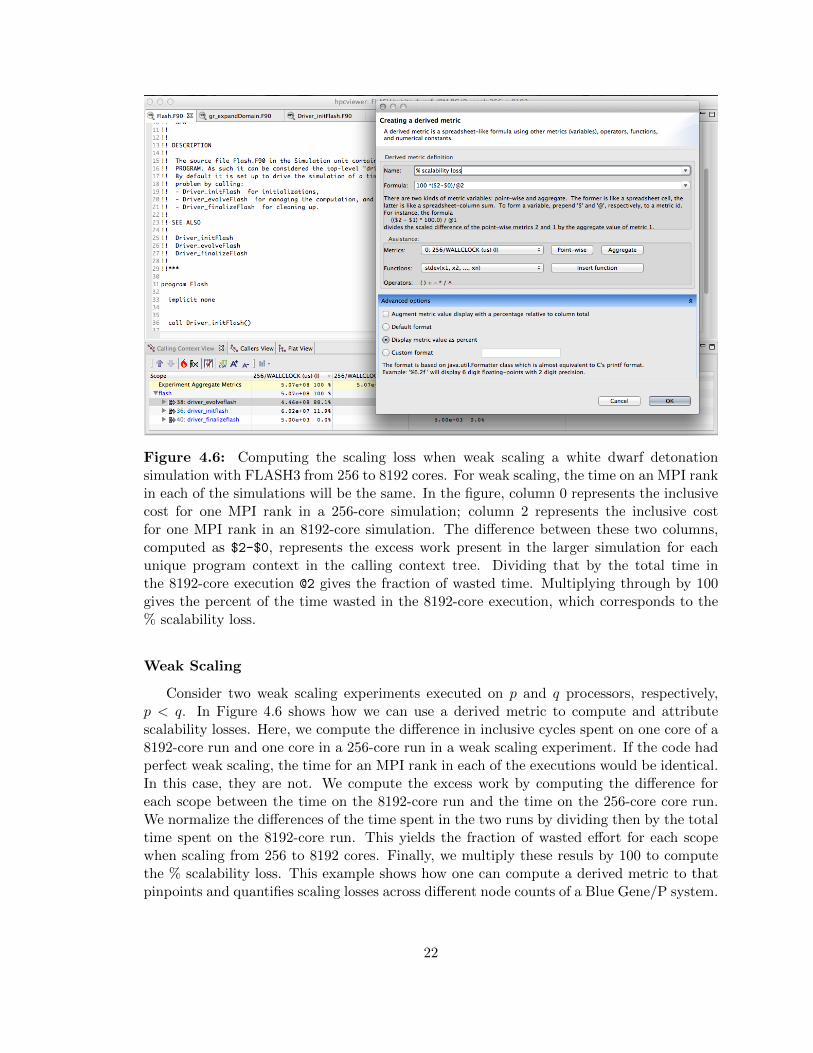
Figure 4.6: Computing the scaling loss when weak scaling a white dwarf detonationsimulation with FLASH3 from 256 to 8192 cores. For weak scaling, the time on an MPI rankin each of the simulations will be the same. In the figure, column 0 represents the inclusivecost for one MPI rank in a 256-core simulation; column 2 represents the inclusive costfor one MPI rank in an 8192-core simulation. The difference between these two columns,computed as $2-$0, represents the excess work present in the larger simulation for eachunique program context in the calling context tree. Dividing that by the total time inthe 8192-core execution @2 gives the fraction of wasted time. Multiplying through by 100gives the percent of the time wasted in the 8192-core execution, which corresponds to the% scalability loss.

Weak Scaling

Consider two weak scaling experiments executed on p and q processors, respectively,p < q. In Figure 4.6 shows how we can use a derived metric to compute and attributescalability losses. Here, we compute the difference in inclusive cycles spent on one core of a8192-core run and one core in a 256-core run in a weak scaling experiment. If the code hadperfect weak scaling, the time for an MPI rank in each of the executions would be identical.In this case, they are not. We compute the excess work by computing the difference foreach scope between the time on the 8192-core run and the time on the 256-core core run.We normalize the differences of the time spent in the two runs by dividing then by the totaltime spent on the 8192-core run. This yields the fraction of wasted effort for each scopewhen scaling from 256 to 8192 cores. Finally, we multiply these resuls by 100 to computethe % scalability loss. This example shows how one can compute a derived metric to thatpinpoints and quantifies scaling losses across different node counts of a Blue Gene/P system.

22

Figure 4.7: Using the fraction the scalability loss metric of Figure 4.6 to rank order loopnests by their scaling loss.

A similar analysis can be applied to compute scaling losses between jobs that use differentnumbers of core counts on individual processors. Figure 4.7 shows the result of computingthe scaling loss for each loop nest when scaling from one to eight cores on a multicore nodeand rank order loop nests by their scaling loss metric. Here, we simply compute the scalingloss as the difference between the cycle counts of the eight-core and the one-core runs,divided through by the aggregate cost of the process executing on eight cores. This figureshows the scaling lost written in scientific notation as a fraction rather than multiplyingthrough by 100 to yield a percent. In this figure, we examine scaling losses in the flat view,showing them for each loop nest. The source pane shows the loop nest responsible for thegreatest scaling loss when scaling from one to eight cores. Unsurprisingly, the loop with theworst scaling loss is very memory intensive. Memory bandwidth is a precious commodityon multicore processors.

While we have shown how to compute and attribute the fraction of excess work in a weakscaling experiment, one can compute a similar quantity for experiments with strong scaling.When differencing the costs summed across all of the threads in a pair of strong-scalingexperiments, one uses exactly the same approach as shown in Figure 4.6. If comparingweak scaling costs summed across all ranks in p and q core executions, one can simply scalethe aggregate costs by 1/p and 1/q respectively before differencing them.

23

Exploring Scaling Losses

Scaling losses can be explored in hpcviewer using any of its three views.

• Calling context view. This top-down view represents the dynamic calling contexts(call paths) in which costs were incurred.

• Callers view. This bottom up view enables one to look upward along call paths. Thisview is particularly useful for understanding the performance of software componentsor procedures that are used in more than one context, such as communication libraryroutines.

• Flat view. This view organizes performance measurement data according to the staticstructure of an application. All costs incurred in any calling context by a procedureare aggregated together in the flat view.

hpcviewer enables developers to explore top-down, bottom-up, and flat views of CCTsannotated with costs, helping to quickly pinpoint performance bottlenecks. Typically, onebegins analyzing an application’s scalability and performance using the top-down callingcontext tree view. Using this view, one can readily see how costs and scalability losses areassociated with different calling contexts. If costs or scalability losses are associated withonly a few calling contexts, then this view suffices for identifying the bottlenecks. Whenscalability losses are spread among many calling contexts, e.g., among different invocationsof MPI_Wait, often it is useful to switch to the bottom-up caller’s view of the data to seeif many losses are due to the same underlying cause. In the bottom-up view, one can sortroutines by their exclusive scalability losses and then look upward to see how these lossesaccumulate from the different calling contexts in which the routine was invoked.

Scaling loss based on excess work is intuitive; perfect scaling corresponds to a excess workvalue of 0, sublinear scaling yields positive values, and superlinear scaling yields negativevalues. Typically, CCTs for SPMD programs have similar structure. If CCTs for differentexecutions diverge, using hpcviewer to compute and report excess work will highlight theseprogram regions.

Inclusive excess work and exclusive excess work serve as useful measures of scalabilityassociated with nodes in a calling context tree (CCT). By computing both metrics, one candetermine whether the application scales well or not at a CCT node and also pinpoint thecause of any lack of scaling. If a node for a function in the CCT has comparable positivevalues for both inclusive excess work and exclusive excess work, then the loss of scalingis due to computation in the function itself. However, if the inclusive excess work for thefunction outweighs that accounted for by its exclusive costs, then one should explore thescalability of its callees. To isolate code that is an impediment to scalable performance, onecan use the hot path button in hpcviewer to trace a path down through the CCT to seewhere the cost is incurred.

24

Chapter 5

Running Applications with hpcrun

and hpclink

This chapter describes the mechanics of using hpcrun and hpclink to profile an appli-cation and collect performance data. For advice on how to choose events, perform scalingstudies, etc., see Chapter 4 Effective Strategies for Analyzing Program Performance.

5.1 Using hpcrun

The hpcrun launch script is used to run an application and collect performance data fordynamically linked binaries. For dynamically linked programs, this requires no change to theprogram source and no change to the build procedure. You should build your applicationnatively at full optimization. hpcrun inserts its profiling code into the application at runtimevia LD_PRELOAD.

The basic options for hpcrun are -e (or --event) to specify a sampling source and rateand -t (or --trace) to turn on tracing. Sample sources are specified as ‘event@period’where event is the name of the source and period is the period (threshold) for that event,and this option may be used multiple times. Note that a higher period implies a lower rateof sampling. The basic syntax for profiling an application with hpcrun is:

hpcrun -t -e event@period ... app arg ...

For example, to profile an application and sample every 15,000,000 total cycles andevery 400,000 L2 cache misses you would use:

hpcrun -e PAPI_TOT_CYC@15000000 -e PAPI_L2_TCM@400000 app arg ...

The units for the WALLCLOCK sample source are in microseconds, so to sample an appli-cation with tracing every 5,000 microseconds (200 times/second), you would use:

hpcrun -t -e WALLCLOCK@5000 app arg ...

hpcrun stores its raw performance data in a measurements directory with the programname in the directory name. On systems with a batch job scheduler (eg, PBS) the name ofthe job is appended to the directory name.

25

hpctoolkit-app-measurements[-jobid]

It is best to use a different measurements directory for each run. So, if you’re usinghpcrun on a local workstation without a job launcher, you can use the ‘-o dirname’ optionto specify an alternate directory name.

For programs that use their own launch script (eg, mpirun or mpiexec for MPI), putthe application’s run script on the outside (first) and hpcrun on the inside (second) on thecommand line. For example,

mpirun -n 4 hpcrun -e PAPI_TOT_CYC@15000000 mpiapp arg ...

Note that hpcrun is intended for profiling dynamically linked binaries. It will not workwell if used to launch a shell script. At best, you would be profiling the shell interpreter,not the script commands, and sometimes this will fail outright.

It is possible to use hpcrun to launch a statically linked binary, but there are two prob-lems with this. First, it is still necessary to build the binary with hpclink. Second, staticbinaries are commonly used on parallel clusters that require running the binary directlyand do not accept a launch script. However, if your system allows it, and if the binarywas produced with hpclink, then hpcrun will set the correct environment variables forprofiling statically or dynamically linked binaries. All that hpcrun really does is set someenvironment variables (including LD_PRELOAD) and exec the binary.

5.2 Using hpclink

For now, see Chapter 9 on Monitoring Statically Linked Applications.

5.3 Sample Sources

This section provide an overview of how to use sample sources supported by HPC-Toolkit. To see a list of the available sample sources and events that hpcrun supports, use‘hpcrun -L’ (dynamic) or set ‘HPCRUN_EVENT_LIST=LIST’ (static). Note that on systemswith separate compute nodes, it is best to run this on one of the compute nodes.

5.3.1 Linux perf events

Linux perf events provides a powerful interface that supports measurement of both ap-plication execution and kernel activity. Using perf events, one can measure both hardwareand software events. Using a processor’s hardware performance monitoring unit (PMU), theperf events interface can measure an execution using any hardware counter supported bythe PMU. Examples of hardware events include cycles, instructions completed, cache misses,and stall cycles. Using instrumentation built in to the Linux kernel, the perf events inter-face can measure software events. Examples of software events include page faults, contextswitches, and CPU migrations.

26

Capabilities of HPCToolkit’s perf events Interface

Frequency-based sampling. Rather than picking a sample period for a hardware counter,the Linux perf events interface enables one to specify the desired sampling frequency andhave the kernel automatically select and adjust the period to try to achieve the desiredsampling frequency.1 To use frequency-based sampling, one can specify the sampling ratefor an event as the desired number of samples per second by prefixing the rate with theletter f. The subsequent subsection on Launching shows some examples of how to monitoran execution using frequency-based sampling.

Multiplexing. Using multiplexing enables one to monitor more events in a single execu-tion than the number of hardware counters a processor can support for each thread. Thenumber of events that can be monitored in a single execution is only limited by the maxi-mum number of concurrent events that the kernel will allow a user to multiplex using theperf events interface.

When more events are specified than can be monitored simultaneously using a thread’shardware counters,2 the kernel will employ multiplexing and divide the set of events to bemonitored into groups, monitor only one group of events at a time, and cycle repeatedlythrough the groups as a program executes.

For applications that have very regular, steady state behavior, e.g., an iterative codewith lots of iterations, multiplexing will yield results that are suitably representative ofexecution behavior. However, for executions that consist of unique short phases, measure-ments collected using multiplexing may not accurately represent the execution behavior.To obtain more accurate measurements, one can run an application multiple times and ineach run collect a subset of events that can be measured without multiplexing. Resultsfrom several such executions can be imported into HPCToolkit’s hpcviewer and analyzedtogether.

Thread blocking. When a program executes, a thread may block waiting for the kernelto complete some operation on its behalf. Example operations include waiting for a read

operation to complete or having the kernel service a page fault or zero-fill a page. On systemsrunning Linux 4.3 or newer, one can use the perf events sample source to monitor howmuch time a thread is blocked and where the blocking occurs. To measure the time a threadspends blocked, one can profile with BLOCKTIME event and another time-based event, suchas CYCLES. The BLOCKTIME event shouldn’t have any frequency or period specified, whereasCYCLES should have a frequency or period specified.

Launching

When sampling with native events, by default hpcrun will profile using perf events.To force HPCToolkit to use PAPI (assuming it's available) instead of perf events, onemust prefix the event with ‘papi::’ as follows:

1The kernel may be unable to deliver the desired frequency if there are fewer events per second than thedesired frequency.

2How many events can be monitored simultaneously on a particular processor may depend on the eventsspecified.

27

hpcrun -e papi::CYCLES

For PAPI presets, there is no need to prefix the event with ‘papi::’. For instance it issufficient to specify PAPI_TOT_CYC event without any prefix to profile using PAPI.

To sample an execution 100 times per second (frequency-based sampling) countingCYCLES and 100 times a second counting INSTRUCTIONS:

hpcrun -e CYCLES@f100 -e INSTRUCTIONS@f100 ...

To sample an execution every 1,000,000 cycles and every 1,000,000 instructions usingperiod-based sampling:

hpcrun -e CYCLES@1000000 -e INSTRUCTIONS@1000000

By default, hpcrun will use frequency-based sampling with the rate 300 samples persecond per event type. Hence the following command will cause HPCToolkit to sampleCYCLES at 300 samples per second and INSTRUCTIONS at 300 samples per second:

hpcrun -e CYCLES -e INSTRUCTIONS

One can a different default rate using the -c option. The command below will sampleCYCLES at 200 samples per second and INSTRUCTIONS at 200 samples per second:

hpcrun -c f200 -e CYCLES -e INSTRUCTIONS

Caveats

• When a system is configured with suitable permissions, HPCToolkit will sample callstacks within the Linux kernel in addition to application-level call stacks. This fea-ture can be useful to diagnose where and why a thread blocks. For this feature tobe available, the file /proc/sys/kernel/perf_event_paranoid file must have value1. To associate addresses in kernel call paths with function names, the value of/proc/sys/kernel/kptr_restrict must be 0 (number zero). If these settings arenot configured in this way on your system, you will need someone with administratorprivileges to change them.

• Due to a limitation of all Linux kernel versions currently available, hpcrun can onlyapproximate a thread’s blocking time using first-party sampling rather than directlymeasuring the time between when a thread blocks and when it resumes.

• Users need to be cautious to compare between different multiplexed counters. Cur-rently, there is no direct information to know if a metric is based on multiplexedcounter. Currently the information is embedded in the experiment.xml file producedwhen post-processing measurement data with hpcprof or hpcprof-mpi, but not vis-ible in the hpcviewer.

28

5.3.2 PAPI

PAPI, the Performance API, is a library for providing access to the hardware perfor-mance counters. This is an attempt to provide a consistent, high-level interface to thelow-level performance counters. PAPI is available from the University of Tennessee at:

http://icl.cs.utk.edu/papi/

PAPI focuses mostly on in-core CPU events: cycles, cache misses, floating point opera-tions, mispredicted branches, etc. For example, the following command samples total cyclesand L2 cache misses.

hpcrun -e PAPI_TOT_CYC@15000000 -e PAPI_L2_TCM@400000 app arg ...

The precise set of PAPI preset and native events is highly system dependent. Commonly,there are events for machine cycles, cache misses, floating point operations and other moresystem specific events. However, there are restrictions both on how many events can besampled at one time and on what events may be sampled together and both restrictions aresystem dependent. Table 5.1 contains a list of commonly available PAPI events.

To see what PAPI events are available on your system, use the papi_avail commandfrom the bin directory in your PAPI installation. The event must be both available andnot derived to be usable for sampling. The command papi_native_avail displays themachine’s native events. Note that on systems with separate compute nodes, you normallyneed to run papi_avail on one of the compute nodes.

When selecting the period for PAPI events, aim for a rate of approximately a fewhundred samples per second. So, roughly several million or tens of million for total cyclesor a few hundred thousand for cache misses. PAPI and hpcrun will tolerate sampling ratesas high as 1,000 or even 10,000 samples per second (or more). But rates higher than a fewthousand samples per second will only drive up the overhead and distort the running ofyour program. It won’t give more accurate results.

Earlier versions of PAPI required a separate patch (perfmon or perfctr) for the Linuxkernel. But beginning with kernel 2.6.32, support for accessing the performance counters(perf events) is now built in to the standard Linux kernel. This means that on kernels 2.6.32or later, PAPI can be compiled and run entirely in user land without patching the kernel.PAPI is highly recommended and well worth building if it is not already installed on yoursystem.

Proxy Sampling HPCToolkit now supports proxy sampling for derived PAPI events.Normally, for HPCToolkit to use a PAPI event, the event must not be derived and mustsupport hardware interrupts. However, for events that cannot trigger interrupts directly,it is still possible to sample on another event and then read the counters for the derivedevents and this is how proxy sampling works. The native events serve as a proxy for thederived events.

To use proxy sampling, specify the hpcrun command line as usual and be sure to includeat least one non-derived PAPI event. The derived events will be counted automaticallyduring the native samples. Normally, you would use PAPI_TOT_CYC as the native event,

29

PAPI_BR_INS Branch instructions

PAPI_BR_MSP Conditional branch instructions mispredicted

PAPI_FP_INS Floating point instructions

PAPI_FP_OPS Floating point operations

PAPI_L1_DCA Level 1 data cache accesses

PAPI_L1_DCM Level 1 data cache misses

PAPI_L1_ICH Level 1 instruction cache hits

PAPI_L1_ICM Level 1 instruction cache misses

PAPI_L2_DCA Level 2 data cache accesses

PAPI_L2_ICM Level 2 instruction cache misses

PAPI_L2_TCM Level 2 cache misses

PAPI_LD_INS Load instructions

PAPI_SR_INS Store instructions

PAPI_TLB_DM Data translation lookaside buffer misses

PAPI_TOT_CYC Total cycles

PAPI_TOT_IIS Instructions issued

PAPI_TOT_INS Instructions completed

Table 5.1: Some commonly available PAPI events. The exact set of available events issystem dependent.

but really this works as long as the event set contains at least one non-derived PAPI event.Proxy sampling only applies to PAPI events, you can’t use itimer as the native event.

For example, on newer Intel CPUs, often the floating point events are all derived andcannot be sampled directly. In that case, you could count flops by using cycles a proxyevent with a command line such as the following. The period for derived events is ignoredand may be omitted.

hpcrun -e PAPI_TOT_CYC@6000000 -e PAPI_FP_OPS app arg ...

Attribution of proxy samples is not as accurate as regular samples. The problem, ofcourse, is that the event that triggered the sample may not be related to the derived counter.The total count of events should be accurate, but their location at the leaves in the CallingContext tree may not be very accurate. However, the higher up the CCT, the more accuratethe attribution becomes. For example, suppose you profile a loop of mixed integer andfloating point operations and sample on PAPI_TOT_CYC directly and count PAPI_FP_OPS viaproxy sampling. The attribution of flops to individual statements within the loop is likelyto be off. But as long as the loop is long enough, the count for the loop as a whole (and upthe tree) should be accurate.

5.3.3 Wallclock, Realtime and Cputime

HPCToolkit supports three timer sample sources: WALLCLOCK, REALTIME and CPUTIME.The WALLCLOCK sample source is based on the ITIMER_PROF interval timer. Normally,PAPI_TOT_CYC is just as good as WALLCLOCK and often better, but WALLCLOCK can be used

30

on systems where PAPI is not available. The units are in microseconds, so the followingexample will sample app approximately 200 times per second.

hpcrun -e WALLCLOCK@5000 app arg ...

Note that the maximum interrupt rate from itimer is limited by the system’s Hz rate,commonly 1,000 cycles per second, but may be lower. That is, WALLCLOCK@10 will notgenerate any higher sampling rate than WALLCLOCK@1000. However, on IBM Blue Gene,itimer is not bound by the Hz rate and so sampling rates faster than 1,000 per second arepossible.

Also, the WALLCLOCK (itimer) signal is not thread-specific and may not work well inthreaded programs. In particular, the number of samples per thread may vary wildly,although this is very system dependent. We recommend not using WALLCLOCK in threadedprograms, except possibly on Blue Gene. Use REALTIME, CPUTIME or PAPI_TOT_CYC instead.

The REALTIME and CPUTIME sources are based on the POSIX timers CLOCK_REALTIME

and CLOCK_THREAD_CPUTIME_ID with the Linux SIGEV_THREAD_ID extension. REALTIME

counts real (wall clock) time, whether the process is running or not, and CPUTIME onlycounts time when the CPU is running. Both units are in microseconds.

REALTIME and CPUTIME are not available on all systems (in particular, not on Blue Gene),but they have important advantages over itimer. These timers are thread-specific and willgive a much more consistent number of samples in a threaded process. Also, compared toitimer, REALTIME includes time when the process is not running and so can identify timeswhen the process is blocked waiting on a syscall. However, REALTIME could also breaksome applications that don’t handle interrupted syscalls well. In that case, consider usingCPUTIME instead.

Note: do not use more than one timer event in the same run. Also, we recommend notusing both PAPI and a timer event together. Technically, this is now possible and hpcrun

won’t fall over. However, PAPI samples would be interrupted by timer signals and viceversa, and this would lead to many dropped samples and possibly distorted results.

5.3.4 IO

The IO sample source counts the number of bytes read and written. This displays twometrics in the viewer: “IO Bytes Read” and “IO Bytes Written.” The IO source is asynchronous sample source. That is, it does not generate asynchronous interrupts. Instead,it overrides the functions read, write, fread and fwrite and records the number of bytesread or written along with their dynamic context.

To include this source, use the IO event (no period). In the static case, two steps areneeded. Use the --io option for hpclink to link in the IO library and use the IO event toactivate the IO source at runtime. For example,

(dynamic) hpcrun -e IO app arg ...

(static) hpclink --io gcc -g -O -static -o app file.c ...

export HPCRUN_EVENT_LIST=IO

app arg ...

31

The IO source is mainly used to find where your program reads or writes large amountsof data. However, it is also useful for tracing a program that spends much time in read

and write. The hardware performance counters (PAPI) do not advance while running inthe kernel, so the trace viewer may misrepresent the amount of time spent in syscalls suchas read and write. By adding the IO source, hpcrun overrides read and write and thusis able to more accurately count the time spent in these functions.

5.3.5 Memleak

The MEMLEAK sample source counts the number of bytes allocated and freed. Like IO,MEMLEAK is a synchronous sample source and does not generate asynchronous interrupts.Instead, it overrides the malloc family of functions (malloc, calloc, realloc and free

plus memalign, posix_memalign and valloc) and records the number of bytes allocatedand freed along with their dynamic context.

MEMLEAK allows you to find locations in your program that allocate memory that isnever freed. But note that failure to free a memory location does not necessarily implythat location has leaked (missing a pointer to the memory). It is common for programs toallocate memory that is used throughout the lifetime of the process and not explicitly freeit.

To include this source, use the MEMLEAK event (no period). Again, two steps are neededin the static case. Use the --memleak option for hpclink to link in the MEMLEAK libraryand use the MEMLEAK event to activate it at runtime. For example,

(dynamic) hpcrun -e MEMLEAK app arg ...

(static) hpclink --memleak gcc -g -O -static -o app file.c ...

export HPCRUN_EVENT_LIST=MEMLEAK

app arg ...

If a program allocates and frees many small regions, the MEMLEAK source may result in ahigh overhead. In this case, you may reduce the overhead by using the memleak probabilityoption to record only a fraction of the mallocs. For example, to monitor 10% of the mallocs,use:

(dynamic) hpcrun -e MEMLEAK --memleak-prob 0.10 app arg ...

(static) export HPCRUN_EVENT_LIST=MEMLEAK

export HPCRUN_MEMLEAK_PROB=0.10

app arg ...

It might appear that if you monitor only 10% of the program’s mallocs, then you wouldhave only a 10% chance of finding the leak. But if a program leaks memory, then it’s likelythat it does so many times, all from the same source location. And you only have to findthat location once. So, this option can be a useful tool if the overhead of recording allmallocs is prohibitive.

Rarely, for some programs with complicated memory usage patterns, the MEMLEAK sourcecan interfere with the application’s memory allocation causing the program to segfault. Ifthis happens, use the hpcrun debug (dd) variable MEMLEAK_NO_HEADER as a workaround.

32

(dynamic) hpcrun -e MEMLEAK -dd MEMLEAK_NO_HEADER app arg ...

(static) export HPCRUN_EVENT_LIST=MEMLEAK

export HPCRUN_DEBUG_FLAGS=MEMLEAK_NO_HEADER

app arg ...

The MEMLEAK source works by attaching a header or a footer to the application’s malloc’dregions. Headers are faster but have a greater potential for interfering with an application.Footers have higher overhead (require an external lookup) but have almost no chance ofinterfering with an application. The MEMLEAK_NO_HEADER variable disables headers and usesonly footers.

5.4 Process Fraction

Although hpcrun can profile parallel jobs with thousands or tens of thousands of pro-cesses, there are two scaling problems that become prohibitive beyond a few thousand cores.First, hpcrun writes the measurement data for all of the processes into a single directory.This results in one file per process plus one file per thread (two files per thread if using trac-ing). Unix file systems are not equipped to handle directories with many tens or hundredsof thousands of files. Second, the sheer volume of data can overwhelm the viewer when thesize of the database far exceeds the amount of memory on the machine.

The solution is to sample only a fraction of the processes. That is, you can run anapplication on many thousands of cores but record data for only a few hundred processes.The other processes run the application but do not record any measurement data. Thisis what the process fraction option (-f or --process-fraction) does. For example, tomonitor 10% of the processes, use:

(dynamic) hpcrun -f 0.10 -e event@period app arg ...

(dynamic) hpcrun -f 1/10 -e event@period app arg ...

(static) export HPCRUN_EVENT_LIST=’event@period’

export HPCRUN_PROCESS_FRACTION=0.10

app arg ...

With this option, each process generates a random number and records its measurementdata with the given probability. The process fraction (probability) may be written as adecimal number (0.10) or as a fraction (1/10) between 0 and 1. So, in the above example,all three cases would record data for approximately 10% of the processes. Aim for a numberof processes in the hundreds.

5.5 Starting and Stopping Sampling

HPCToolkit supports an API for the application to start and stop sampling. Thisis useful if you want to profile only a subset of a program and ignore the rest. The APIsupports the following functions.

void hpctoolkit_sampling_start(void);

void hpctoolkit_sampling_stop(void);

33

For example, suppose that your program has three major phases: it reads input froma file, performs some numerical computation on the data and then writes the output toanother file. And suppose that you want to profile only the compute phase and skip theread and write phases. In that case, you could stop sampling at the beginning of theprogram, restart it before the compute phase and stop it again at the end of the computephase.

This interface is process wide, not thread specific. That is, it affects all threads of aprocess. Note that when you turn sampling on or off, you should do so uniformly across allprocesses, normally at the same point in the program. Enabling sampling in only a subsetof the processes would likely produce skewed and misleading results.

And for technical reasons, when sampling is turned off in a threaded process, interruptsare disabled only for the current thread. Other threads continue to receive interrupts, butthey don’t unwind the call stack or record samples. So, another use for this interface isto protect syscalls that are sensitive to being interrupted with signals. For example, someGemini interconnect (GNI) functions called from inside gasnet_init() or MPI_Init() onCray XE systems will fail if they are interrupted by a signal. As a workaround, you couldturn sampling off around those functions.

Also, you should use this interface only at the top level for major phases of your program.That is, the granularity of turning sampling on and off should be much larger than the timebetween samples. Turning sampling on and off down inside an inner loop will likely produceskewed and misleading results.

To use this interface, put the above function calls into your program where you wantsampling to start and stop. Remember, starting and stopping apply process wide. ForC/C++, include the following header file from the HPCToolkit include directory.

#include <hpctoolkit.h>

Compile your application with libhpctoolkit with -I and -L options for the includeand library paths. For example,

gcc -I /path/to/hpctoolkit/include app.c ... \

-L /path/to/hpctoolkit/lib/hpctoolkit -lhpctoolkit ...

The libhpctoolkit library provides weak symbol no-op definitions for the start andstop functions. For dynamically linked programs, be sure to include -lhpctoolkit on thelink line (otherwise your program won’t link). For statically linked programs, hpclink

adds strong symbol definitions for these functions. So, -lhpctoolkit is not necessary inthe static case, but it doesn’t hurt.

To run the program, set the LD_LIBRARY_PATH environment variable to include theHPCToolkit lib/hpctoolkit directory. This step is only needed for dynamically linkedprograms.

export LD_LIBRARY_PATH=/path/to/hpctoolkit/lib/hpctoolkit

Note that sampling is initially turned on until the program turns it off. If you want itinitially turned off, then use the -ds (or --delay-sampling) option for hpcrun (dynamic)or set the HPCRUN_DELAY_SAMPLING environment variable (static).

34

(dynamic) hpcrun -ds -e event@period app arg ...

(static) export HPCRUN_EVENT_LIST=’event@period’

export HPCRUN_DELAY_SAMPLING=1

app arg ...

5.6 Environment Variables for hpcrun

For most systems, hpcrun requires no special environment variable settings. There aretwo situations, however, where hpcrun, to function correctly, must refer to environmentvariables. These environment variables, and corresponding situations are:

HPCTOOLKIT To function correctly, hpcrun must know the location of the HPCToolkittop-level installation directory. The hpcrun script uses elements of the installationlib and libexec subdirectories. On most systems, the hpcrun can find the requisitecomponents relative to its own location in the file system. However, some parallel joblaunchers copy the hpcrun script to a different location as they launch a job. If yoursystem does this, you must set the HPCTOOLKIT environment variable to the locationof the HPCToolkit top-level installation directory before launching a job.

Note to system administrators: if your system provides a module system for con-figuring software packages, then constructing a module for HPCToolkit to initialize theseenvironment variables to appropriate settings would be convenient for users.

5.7 Platform-Specific Notes

5.7.1 Cray XE6 and XK6

The ALPS job launcher used on Cray XE6 and XK6 systems copies programs to a specialstaging area before launching them, as described in Section 5.6. Consequently, when usinghpcrun to monitor dynamically linked binaries on Cray XE6 and XK6 systems, you shouldadd the HPCTOOLKIT environment variable to your launch script. Set HPCTOOLKIT to thetop-level HPCToolkit installation directory (the directory containing the bin, lib andlibexec subdirectories) and export it to the environment. (If launching statically-linkedbinaries created using hpclink, this step is unnecessary, but harmless.) Below we showa skeletal job script that sets the HPCTOOLKIT environment variable before monitoring adynamically-linked executable with hpcrun:

#!/bin/sh

#PBS -l mppwidth=#nodes

#PBS -l walltime=00:30:00

#PBS -V

export HPCTOOLKIT=/path/to/hpctoolkit/install/directory

export CRAY_ROOTFS=DSL

cd $PBS_O_WORKDIR

aprun -n #nodes hpcrun -e event@period dynamic-app arg ...

35

If HPCTOOLKIT is not set, you may see errors such as the following in your job’s errorlog.

/var/spool/alps/103526/hpcrun: Unable to find HPCTOOLKIT root directory.

Please set HPCTOOLKIT to the install prefix, either in this script,

or in your environment, and try again.

The problem is that the Cray job launcher copies the hpcrun script to a directorysomewhere below /var/spool/alps/ and runs it from there. By moving hpcrun to adifferent directory, this breaks hpcrun’s method for finding its own install directory. Thesolution is to add HPCTOOLKIT to your environment so that hpcrun can find its installdirectory.

Your system may have a module installed for hpctoolkit with the correct settings forPATH, HPCTOOLKIT, etc. In that case, the easiest solution is to load the hpctoolkit module.Try “module show hpctoolkit” to see if it sets HPCTOOLKIT.

36

Chapter 6

hpcviewer’s User Interface

HPCToolkit provides the hpcviewer [2] performance presentation tool for interactiveexamination of performance databases. hpcviewer interactively presents context-sensitiveperformance metrics correlated to program structure and mapped to a program’s sourcecode, if available. It can present an arbitrary collection of performance metrics gatheredduring one or more runs or compute derived metrics.

6.1 Launching

hpcviewer can either be launched from a command line (Linux/Unix platform) or byclicking the hpcviewer icon (for Windows, Mac OS X and Linux/Unix platform). Thecommand line syntax is as follows:

hpcviewer [options] [<hpctoolkit-database>]

Here, <hpctoolkit-database> is an optional argument to load a database automatically.Without this argument, hpcviewer will prompt for the location of a database.

The possible options are as follows:

• -n: Do not display the Callers View. (May save memory and time.)

• -consolelog: Send log entries to a console in addition to a log file. (To get a consolewindow, be sure to use java as the VM instead of javaw.)

• -debug: Log additional information about plug-in dependency problems.

6.2 Views

Figure 6.1 shows an annotated screenshot of hpcviewer’s user interface presenting acall path profile. The annotations highlight hpcviewer’s principal window panes and keycontrols. The browser window is divided into three panes. The Source pane (top) displaysprogram source code. The Navigation and Metric panes (bottom) associate a table ofperformance metrics with static or dynamic program structure. These panes are discussedin more detail in Section 6.3.

37

Figure 6.1: An annotated screenshot of hpcviewer’s interface.

hpcviewer displays calling-context-sensitive performance data in three different views:a top-down Calling Context View, a bottom-up Callers View, and a Flat View. One selectsthe desired view by clicking on the corresponding view control tab. We briefly describe thethree views and their corresponding purposes.

• Calling Context View. This top-down view represents the dynamic calling contexts(call paths) in which costs were incurred. Using this view, one can explore performancemeasurements of an application in a top-down fashion to understand the costs incurredby calls to a procedure in a particular calling context. We use the term cost rather thansimply time since hpcviewer can present a multiplicity of measured such as cycles, orcache misses) or derived metrics (e.g. cache miss rates or bandwidth consumed) thatthat are other indicators of execution cost.

A calling context for a procedure f consists of the stack of procedure frames activewhen the call was made to f. Using this view, one can readily see how much of the ap-plication’s cost was incurred by f when called from a particular calling context. If finerdetail is of interest, one can explore how the costs incurred by a call to f in a partic-ular context are divided between f itself and the procedures it calls. HPCToolkit’s

38

call path profiler hpcrun and the hpcviewer user interface distinguish calling contextprecisely by individual call sites; this means that if a procedure g contains calls toprocedure f in different places, these represent separate calling contexts.

• Callers View. This bottom-up view enables one to look upward along call paths.The view apportions a procedure’s costs to its caller and, more generally, its callingcontexts. This view is particularly useful for understanding the performance of soft-ware components or procedures that are used in more than one context. For instance,a message-passing program may call MPI_Wait in many different calling contexts.The cost of any particular call will depend upon the structure of the parallelizationin which the call is made. Serialization or load imbalance may cause long waits insome calling contexts while other parts of the program may have short waits becausecomputation is balanced and communication is overlapped with computation.

When several levels of the Callers View are expanded, saying that the Callers Viewapportions metrics of a callee on behalf of its caller can be confusing: what is thecaller and what is the callee? In this situation, we can say that the Callers View ap-portions the metrics of a particular procedure in its various calling contexts on behalfof that context’s caller. Alternatively but equivalently, the Callers View apportionsthe metrics of a particular procedure on behalf of its various calling contexts.

• Flat View. This view organizes performance measurement data according to thestatic structure of an application. All costs incurred in any calling context by aprocedure are aggregated together in the Flat View. This complements the CallingContext View, in which the costs incurred by a particular procedure are representedseparately for each call to the procedure from a different calling context.

6.3 Panes

hpcviewer’s browser window is divided into three panes: the Navigation pane, Sourcepane, and the Metrics pane. We briefly describe the role of each pane.

6.3.1 Source pane

The source pane displays the source code associated with the current entity selectedin the navigation pane. When a performance database is first opened with hpcviewer,the source pane is initially blank because no entity has been selected in the navigationpane. Selecting any entity in the navigation pane will cause the source pane to load thecorresponding file, scroll to and highlight the line corresponding to the selection. Switchingthe source pane to view to a different source file is accomplished by making another selectionin the navigation pane.

6.3.2 Navigation pane

The navigation pane presents a hierarchical tree-based structure that is used to organizethe presentation of an applications’s performance data. Entities that occur in the navigationpane’s tree include load modules, files, procedures, procedure activations, inlined code,

39

loops, and source lines. Selecting any of these entities will cause its corresponding sourcecode (if any) to be displayed in the source pane. One can reveal or conceal children in thishierarchy by ‘opening’ or ‘closing’ any non-leaf (i.e., individual source line) entry in thisview.

The nature of the entities in the navigation pane’s tree structure depends upon whetherone is exploring the Calling Context View, the Callers View, or the Flat View of theperformance data.

• In the Calling Context View, entities in the navigation tree represent procedureactivations, inlined code, loops, and source lines. While most entities link to a singlelocation in source code, procedure activations link to two: the call site from which aprocedure was called and the procedure itself.

• In the Callers View, entities in the navigation tree are procedure activations. Unlikeprocedure activations in the calling context tree view in which call sites are pairedwith the called procedure, in the caller’s view, call sites are paired with the callingprocedure to facilitate attribution of costs for a called procedure to multiple differentcall sites and callers.

• In the Flat View, entities in the navigation tree correspond to source files, procedurecall sites (which are rendered the same way as procedure activations), loops, andsource lines.

Navigation control

The header above the navigation pane contains some controls for the navigation andmetric view. In Figure 6.1, they are labeled as “navigation/metric control.”

• Flatten / Unflatten (available for the Flat View):

Enabling to flatten and unflatten the navigation hierarchy. Clicking on the flattenbutton (the icon that shows a tree node with a slash through it) will replace eachtop-level scope shown with its children. If a scope has no children (i.e., it is a leaf ),the node will remain in the view. This flattening operation is useful for relaxing thestrict hierarchical view so that peers at the same level in the tree can be viewed andranked together. For instance, this can be used to hide procedures in the Flat Viewso that outer loops can be ranked and compared to one another. The inverse of theflatten operation is the unflatten operation, which causes an elided node in the treeto be made visible once again.

• Zoom-in / Zoom-out :

Depressing the up arrow button will zoom in to show only information for the selectedline and its descendants. One can zoom out (reversing a prior zoom operation) bydepressing the down arrow button.

• Hot call path :

This button is used to automatically find hot call paths with respect to the currentlyselected metric column. The hot path is computed by comparing parent and child

40

Figure 6.2: Context menu in the navigation pane: activated by clicking the right-buttonof the mouse.

metric values, and showing the chain where the difference is greater than a threshold(by default is 50%). It is also possible to change the threshold value by clicking themenu File—Preference.

• Derived metric :

Creating a new metric based on mathematical formula. See Section 6.5 for moredetails.

• Hide/show metrics :

Showing and hiding metric columns. A dialog box will appear, and user can selectwhich columns to show or hide. See Section 6.8.2 section for more details.

• Export into a CSV format file :

Exporting the current metric table into a comma separated value (CSV) format file.This feature only exports all metrics that are currently shown. Metrics that are notshown in the view (whose scopes are not expanded) will not be exported (we assumethese metrics are not significant).

• Increase font size / Decrease font size :

Increasing or decreasing the size of the navigation and metric panes.

• Showing graph of metric values :

Showing the graph (plot, sorted plot or histogram) of metric values of the selectednode in CCT for all processes or threads (Section 6.6.1). This menu is only availableif the database is generated by hpcprof-mpi instead of hpcprof.

• Show the metrics of a set of threads :

Showing the CCT and the metrics of a seletected threads (Section 6.6.2). This menuis only available if the database is generated by hpcprof-mpi instead of hpcprof.

Context menus

Navigation control also provides several context menus by clicking the right-button ofthe mouse. As shown in Figure 6.2, the menus are:

41

• Zoom-in/out: Carrying out exactly the same as action as the Zoom-in/out in thenavigation control.

• Copy: Copying into clipboard the selected line in navigation pane which includes thename of the node in the tree, and the values of visible metrics in metric pane (Section6.3.3). The values of hidden metrics will not be copied.

• Show ...: Showing the source code file and highlighting the specified line in (SectionSource pane 6.3.1). If the file doesn’t exist, the menu is disabled.

• Callsite ...: Showing the source code file and highlighting the specified line of thecall site. This menu only available in Calling Context View. If the file doesn’t exist,the menu is disabled.

• Graph ...: Showing the graph (plot, sorted plot or histogram) of metric values of theselected node in CCT for all processes or threads (Section 6.6.1). This menu is onlyavailable if the database is generated by hpcprof-mpi instead of hpcprof.

6.3.3 Metric pane

The metric pane displays one or more performance metrics associated with entities tothe left in the navigation pane. Entities in the tree view of the navigation pane are sortedat each level of the hierarchy by the metric in the selected column. When hpcviewer islaunched, the leftmost metric column is the default selection and the navigation pane issorted according to the values of that metric in descending order. One can change theselected metric by clicking on a column header. Clicking on the header of the selectedcolumn toggles the sort order between descending and ascending.

During analysis, one often wants to consider the relationship between two metrics. Thisis easier when the metrics of interest are in adjacent columns of the metric pane. One canchange the order of columns in the metric pane by selecting the column header for a metricand then dragging it left or right to its desired position. The metric pane also includesscroll bars for horizontal scrolling (to reveal other metrics) and vertical scrolling (to revealother scopes). Vertical scrolling of the metric and navigation panes is synchronized.

6.4 Understanding Metrics

hpcviewer can present an arbitrary collection of performance metrics gathered duringone or more runs, or compute derived metrics expressed as formulae with existing metricsas terms.

For any given scope in hpcviewer’s three views, hpcviewer computes both inclusiveand exclusive metric values. For the moment, consider the Calling Context View. Inclusivemetrics reflect costs for the entire subtree rooted at that scope. Exclusive metrics are of twoflavors, depending on the scope. For a procedure, exclusive metrics reflect all costs withinthat procedure but excluding callees. In other words, for a procedure, costs are exclusivewith respect to dynamic call chains. For all other scopes, exclusive metrics reflect costs forthe scope itself; i.e., costs are exclusive with respect to static structure. The Callers andFlat Views contain inclusive and exclusive metric values that are relative to the Calling

42

file1.c file2.c

f () {

g ();

}

// m is the main routine

m () {

f ();

g ();

}

// g can be a recursive function

g () {

if ( . . ) g ();

if ( . . ) h ();

}

h () {

}

Figure 6.3: A sample program divided into two source files.

Context View. This means, e.g., that inclusive metrics for a particular scope in the Callersor Flat View are with respect to that scope’s subtree in the Calling Context View.

6.4.1 How metrics are computed?

Call path profile measurements collected by hpcrun correspond directly to the CallingContext View. hpcviewer derives all other views from exclusive metric costs in the CallingContext View. For the Caller View, hpcviewer collects the cost of all samples in eachfunction and attribute that to a top-level entry in the Caller View. Under each top-levelfunction, hpcviewer can look up the call chain at all of the context in which the function iscalled. For each function, hpcviewer apportions its costs among each of the calling contextsin which they were incurred. hpcviewer computes the Flat View by traversing the callingcontext tree and attributing all costs for a scope to the scope within its static source codestructure. The Flat View presents a hierarchy of nested scopes for load modules, files,procedures, loops, inlined code and statements.

6.4.2 Example

Figure 6.3 shows an example of a recursive program separated into two files, file1.cand file2.c. In this figure, we use numerical subscripts to distinguish between differ-ent instances of the same procedure. In the other parts of this figure, we use alphabeticsubscripts. We use different labels because there is no natural one-to-one correspondencebetween the instances in the different views.

Routine g can behave as a recursive function depending on the value of the conditionbranch (lines 3–4). Figure 6.4 shows an example of the call chain execution of the programannotated with both inclusive and exclusive costs. Computation of inclusive costs fromexclusive costs in the Calling Context View involves simply summing up all of the costs inthe subtree below.

In this figure, we can see that on the right path of the routine m, routine g (instantiatedin the diagram as g1) performed a recursive call (g2) before calling routine h. Although

43

Figure 6.4: Calling Context View. Each node of the tree has three boxes: the left-mostis the name of the node (or in this case the name of the routine, the center is the inclusivevalue, and on the right is the exclusive value.

Figure 6.5: Caller View

g1, g2 and g3 are all instances from the same routine (i.e., g), we attribute a different costfor each instance. This separation of cost can be critical to identify which instance has aperformance problem.

Figure 6.5 shows the corresponding scope structure for the Caller View and the costswe compute for this recursive program. The procedure g noted as ga (which is a root node

Figure 6.6: Flat View

44

in the diagram), has different cost to g as a callsite as noted as gb, gc and gd. For instance,on the first tree of this figure, the inclusive cost of ga is 9, which is the sum of the highestcost for each branch in calling context tree (Figure 6.4): the inclusive cost of g3 (which is3) and g1 (which is 6). We do not attribute the cost of g2 here since it is a descendant ofg1 (in other term, the cost of g2 is included in g1).

Inclusive costs need to be computed similarly in the Flat View. The inclusive cost of arecursive routine is the sum of the highest cost for each branch in calling context tree. Forinstance, in Figure 6.6, The inclusive cost of gx, defined as the total cost of all instancesof g, is 9, and this is consistently the same as the cost in caller tree. The advantage ofattributing different costs for each instance of g is that it enables a user to identify whichinstance of the call to g is responsible for performance losses.

6.5 Derived Metrics

Frequently, the data become useful only when combined with other information suchas the number of instructions executed or the total number of cache accesses. While usersdon’t mind a bit of mental arithmetic and frequently compare values in different columnsto see how they relate for a scope, doing this for many scopes is exhausting. To addressthis problem, hpcviewer provides a mechanism for defining metrics. A user-defined metricis called a “derived metric.” A derived metric is defined by specifying a spreadsheet-likemathematical formula that refers to data in other columns in the metric table by using $nto refer to the value in the nth column.

6.5.1 Formulae

The formula syntax supported by hpcviewer is inspired by spreadsheet-like in-fix math-ematical formulae. Operators have standard algebraic precedence.

6.5.2 Examples

Suppose the database contains information about 5 processes, each with two metrics:

1. Metric 0, 2, 4, 6 and 8: total number of cycles

2. Metric 1, 3, 5, 7 and 9: total number of floating point operations

To compute the average number of cycles per floating point operation across all of theprocesses, we can define a formula as follows:

avg($0, $2, $4. $6. $8) / avg($1, $3, $5, $7, $9)

6.5.3 Derived metric dialog box

A derived metric can be created by clicking the Derived metric tool item in thenavigation/control pane. A derived metric window will then appear as shown in Figure 6.7.

The window has two main parts:

• Derived metric definition, which consists of:

45

Figure 6.7: Derived metric dialog box

– New name for the derived metric. Supply a string that will be used as the columnheader for the derived metric. If you don’t supply one, the metric will have noname.

– Formula definition field. In this field the user can define a formula with spreadsheet-like mathematical formula. This field is required to be filled.

– Metric help. This is used to help the user to find the ID of a metric. Forinstance, in this snapshot, the metric PAPI TOT CYC has the ID 44. By clickingthe button Insert metric, the metric ID will be inserted in formula definitionfield.

– Function help. This help is to guide the user to insert functions in the formuladefinition field. Some functions require only one metric as the argument, butsome can have two or more arguments. For instance, the function avg() whichcomputes the average of some metrics, need to have two arguments.

• Advanced options:

– Augment metric value display with a percentage relative to column total. Whenthis box is checked, each scope’s derived metric value will be augmented with a

46

percentage value, which for scope s is computed as the 100 * (s’s derived metricvalue) / (the derived metric value computed by applying the metric formula to theaggregate values of the input metrics) the entire execution). Such a computationcan lead to nonsensical results for some derived metric formulae. For instance, ifthe derived metric is computed as a ratio of two other metrics, the aforementionedcomputation that compares the scope’s ratio with the ratio for the entire programwon’t yield a meaningful result. To avoid a confusing metric display, think beforeyou use this button to annotate a metric with its percent of total.

– Default format. This option will set the metric value with a scientific notationformat which is the default format.

– Display metric value as percent. This option will set the metric value with percentformat. For instance, if the metric has a value 12.345678, with this option, it’sdisplayed as 12.34%.

– Custom format. This option will set the metric value with your customizedformat. The format is equivalent to Java’s Formatter class, or similar to C’sprintf format. For example, the format ”%6.2f” will display 6 digit floating-points with 2 digit precision.

Note that the entered formula and the metric name will be stored automatically. Onecan then review again the formula (or metric name) by clicking the small triangle of thecombo box (marked with a red circle).

6.6 Thread-level Metric Values

6.6.1 Plotting graphs

HPCToolkit Experiment databases that have been generated by hpcprof-mpi (incontrast to hpcprof) can be used by hpcviewer to plot graphs of thread-level metric values.This is particularly useful for quickly assessing load imbalance in context across the severalthreads or processes of an execution. Figure 6.8 shows hpcviewer rendering such a plot.The horizontal axis shows application processes, ordered by MPI rank. The vertical axisshows metric values for each process. Because hpcviewer can generate scatter plots for anynode in the Calling Context View, these graphs are calling-context sensitive.

To create a graph, first select a scope in the Calling Context View; in the Figure, the top-level procedure main is selected. Then, right-click the selected scope to show the associatedcontext menu. (The menu begins with entries labeled ‘Zoom-in’ and ‘Zoom-out.’) At thebottom of the context menu is a list of metrics that hpcviewer can graph. Each metriccontains a sub-menu that lists the three different types of graphs hpcviewer can plot:

• Plot graph. This standard graph plots metric values by their MPI rank (if available)and thread id (where ids are assigned by thread creation).

• Sorted plot graph. This graph plots metric values in ascending order.

• Histogram graph. This graph is a histogram of metric values. It divides the rangeof metric values into a small number of sub-ranges. The graph plots the frequencythat a metric value falls into a particular sub-range.

47

Figure 6.8: Plot graph view of main procedure in a Coarray Fortran application.

Note that the viewers have the following notation for the ranks:

<process_id> . <thread_id>

Hence, if the ranks are 0.0, 0.1, . . . 31.0, 31.1 it means MPI process 0 has two threads:thread 0 and thread 1 (similarly with MPI process 31).

Currently, it is only possible to generate scatter plots for metrics directly collected byhpcrun, which excludes derived metrics created within hpcviewer.

6.6.2 Thread View

hpcviewer also provides a feature to view the metrics of a certain threads (or processes)named Thread View. First, you need to select a thread or a set of threads of interest. Toselect a single thread, you can click on the dot from the plot graph (see Figure 6.8). Thenclick the context menu “Show thread X” to activate the thread view.

To select a group of threads, you need to use the thread selection window by clickingbutton from the calling-context view. On the thread selection window, you need to selectthe checkbox of the threads of interest. To narrow the list, you can specify the thread nameon the filter part of the window. Recall that the format of the thread is “process id .

thread id” (see Section 6.6). Hence, to specify just a main thread (thread zero), you cantype ’.0’ on the filter, and the view only list threads 0 (such as 1.0, 2.0, 3.0 . . . ).

Once threads have been selected, you can click OK, and the Thread view (Figure 6.9)will be activated. The tree of the view is the same as the tree from calling context view,

48

Figure 6.9: Example of a Thread View which display thread-level metrics of a set ofthreads. The first column is a CCT equivalent to the CCT in the Calling Context View,the second and third columns represent the metrics of the selected threads (in this case theyare threads from 0.0, to 15.0)

with the metrics only from the selected threads. If there are more than one selected threads,the metrics are the average of the values of the selected threads.

6.7 Filtering Tree nodes

Occasionally, It is useful to omit uninterested nodes in the CCT and to focus on impor-tant parts. For instance, you may want to hide all nodes associated with OpenMP runtimeand just show all nodes and metrics from the application. For this purpose, hpcviewer pro-vides filtering to elide nodes that match a filter pattern. hpcviewer allows users to definemultiple filters, and each filter is associated with a glob pattern 1 and a type. There arethree types of filter: “self only” to omit the matched nodes, “descendants only” to excludeonly the subtree of the matched nodes, and “self and descendants” to remove the matchednodes and its descendants.

Self only : This filter is useful to hide intermediary runtime functions such as pthreador OpenMP runtime functions. All nodes that match filter patterns will be removed, andtheir children will be augmented to the parent of the elided nodes. The exclusive cost ofthe elided nodes will be also augmented into the exclusive cost of the parent of the elidednodes. Figure 6.10b shows the result of filtering node C of the CCT from Figure 6.10a.Node C is elided and its exclusive cost is augmented into the exclusive cost of its parent(node A). The children of node C (nodes D and E) are now the children of node A.

1A glob pattern specifies which name to be removed by using wildcard characters such as *, ? and +

49

(a) The original CCT tree.

(b) The result of applying self only filteron node C. Node C is elided and its children(nodes D and E) are augmented to the parentof node C. The exclusive cost of node C is alsoaugmented to node A.

(c) The result of applying Descendants onlyfilter on node C. All the children of node C

(nodes D and E) are elided, and the total oftheir exclusive cost is added to node C.

(d) The result of applying self and descen-dants filter on node C. Nodes C and its de-scendants are elided, and their exclusive costis augmented to node A which is the parentof node C.

Figure 6.10: Different results of filtering on node C from Figure 6.10a (the original CCT).Figure 6.10b shows the result of self only filter, Figure 6.10c shows the result of descendantsonly filter, and Figure 6.10d shows the result of self and descendants filter. Each node isattributed with two boxes on its right. The left box represents the node’s inclusive cost,while the right box represents the exclusive cost.

Figure 6.11: The window of filter property.

50

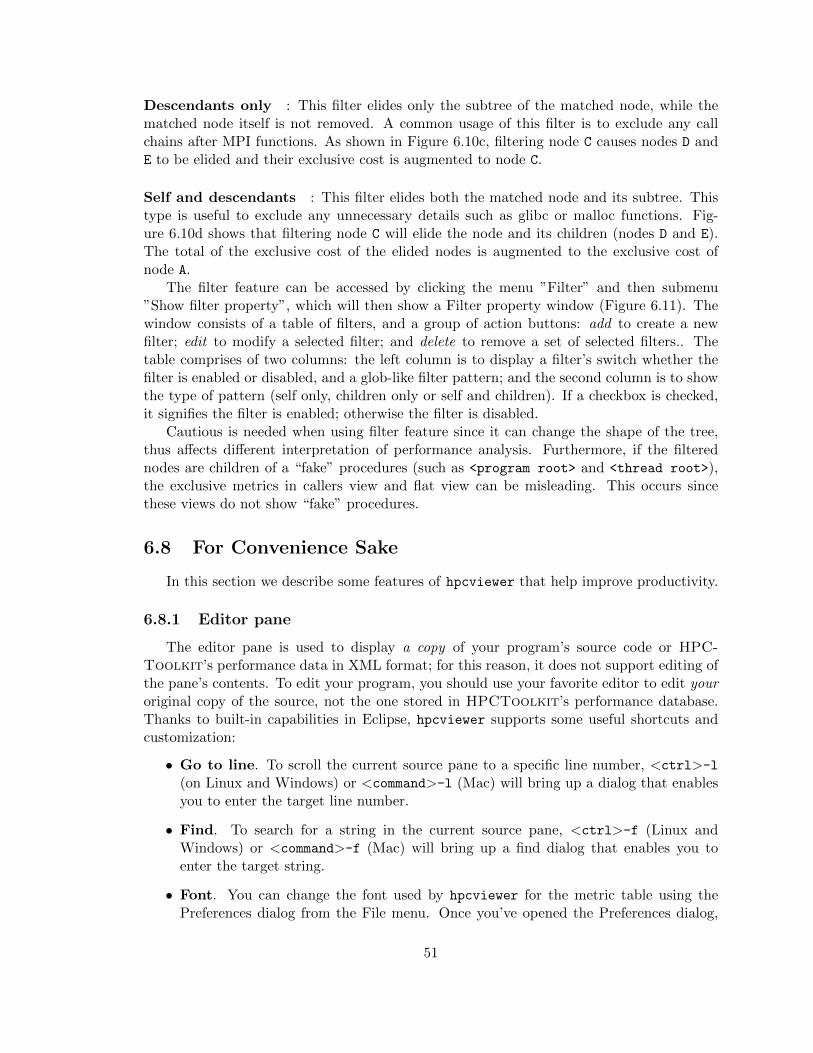
Descendants only : This filter elides only the subtree of the matched node, while thematched node itself is not removed. A common usage of this filter is to exclude any callchains after MPI functions. As shown in Figure 6.10c, filtering node C causes nodes D andE to be elided and their exclusive cost is augmented to node C.

Self and descendants : This filter elides both the matched node and its subtree. Thistype is useful to exclude any unnecessary details such as glibc or malloc functions. Fig-ure 6.10d shows that filtering node C will elide the node and its children (nodes D and E).The total of the exclusive cost of the elided nodes is augmented to the exclusive cost ofnode A.

The filter feature can be accessed by clicking the menu ”Filter” and then submenu”Show filter property”, which will then show a Filter property window (Figure 6.11). Thewindow consists of a table of filters, and a group of action buttons: add to create a newfilter; edit to modify a selected filter; and delete to remove a set of selected filters.. Thetable comprises of two columns: the left column is to display a filter’s switch whether thefilter is enabled or disabled, and a glob-like filter pattern; and the second column is to showthe type of pattern (self only, children only or self and children). If a checkbox is checked,it signifies the filter is enabled; otherwise the filter is disabled.

Cautious is needed when using filter feature since it can change the shape of the tree,thus affects different interpretation of performance analysis. Furthermore, if the filterednodes are children of a “fake” procedures (such as <program root> and <thread root>),the exclusive metrics in callers view and flat view can be misleading. This occurs sincethese views do not show “fake” procedures.

6.8 For Convenience Sake

In this section we describe some features of hpcviewer that help improve productivity.

6.8.1 Editor pane

The editor pane is used to display a copy of your program’s source code or HPC-Toolkit’s performance data in XML format; for this reason, it does not support editing ofthe pane’s contents. To edit your program, you should use your favorite editor to edit youroriginal copy of the source, not the one stored in HPCToolkit’s performance database.Thanks to built-in capabilities in Eclipse, hpcviewer supports some useful shortcuts andcustomization:

• Go to line. To scroll the current source pane to a specific line number, <ctrl>-l(on Linux and Windows) or <command>-l (Mac) will bring up a dialog that enablesyou to enter the target line number.

• Find. To search for a string in the current source pane, <ctrl>-f (Linux andWindows) or <command>-f (Mac) will bring up a find dialog that enables you toenter the target string.

• Font. You can change the font used by hpcviewer for the metric table using thePreferences dialog from the File menu. Once you’ve opened the Preferences dialog,

51

select hpcviewer preferences (the item at the bottom of the list in the column on theleft side of the pane). The new font will take effect when you next launch hpcviewer.

• Minimize/Maximize window. Icons in the upper right corner of the window enable

you to minimize ( ) or maximize ( ) the hpcviewer window.

6.8.2 Metric pane

For the metric pane, hpcviewer has some convenient features:

• Maximizing a view. To expand the source or metric pane to fill the window, onecan double click on the tab with the view name. Double clicking again on the viewname will restore the view back to its original size.

• Sorting the metric pane contents by a column’s values. First, select the columnon which you wish to sort. If no triangle appears next to the metric, click again. Adownward pointing triangle means that the rows in the metric pane are sorted indescending order according to the column’s value. Additional clicks on the header ofthe selected column will toggle back and forth between ascending and descending.

• Changing column width. To increase or decrease the width of a column, first putthe cursor over the right or left border of the column’s header field. The cursor willchange into a vertical bar between a left and right arrow. Depress the mouse and dragthe column border to the desired position.

• Changing column order. If it would be more convenient to have columns displayedin a different order, they can be permuted as you wish. Depress and hold the mousebutton over the header of column that you wish to move and drag the column rightor left to its new position.

• Copying selected metrics into clipboard. In order to copy selected lines ofscopes/metrics, one can right click on the metric pane or navigation pane then selectthe menu Copy. The copied metrics can then be pasted into any text editor.

• Hiding or showing metric columns. Sometimes, it may be more convenient tosuppress the display of metrics that are not of current interest. When there are toomany metrics to fit on the screen at once, it is often useful to suppress the display ofsome. The icon above the metric pane will bring up the column selection dialogshown in Figure 6.12.

The dialog box contains a list of metric columns sorted according to their order inHPCToolkit’s performance database for the application. Each metric column isprefixed by a check box to indicate if the metric should be displayed (if checked)or hidden (unchecked). To display all metric columns, one can click the Check allbutton. A click to Uncheck all will hide all the metric columns.

Finally, an option Apply to all views will set the configuration into all views whenchecked. Otherwise, the configuration will be applied only on the current view.

52

Figure 6.12: Hide/Show columns dialog box

6.9 Menus

hpcviewer provides five main menus:

6.9.1 File

This menu includes several menu items for controlling basic viewer operations.

• New window Open a new hpcviewer window that is independent from the existingone.

• Open database... Load a performance database into the current hpcviewer window.Currently hpcviewer restricts maximum of five database open at a time. If you wantto display more than five, either you close an existing open database first, or you opena new hpcviewer window.

• Close database... Unloading one of more open performance database.

• Merge database CCT.../Merge database flat tree... Merging two databasethat are currently in the viewer. If hpcviewer has more than two open database,then you need to choose which database you want to merge.

Currently hpcviewer does not support storing a merged database into a file.

• Preferences... Display the settings dialog box.

• Close window Closing the current window. If there is only one window, then thismenu will also exit hpcviewer application.

• Exit Quit the hpcviewer application.

53

6.9.2 Filter

This menu only contains one submenu:

• Show filter property Open a filter property window which lists a set of filters andits properties (Section 6.7).

6.9.3 View

This menu is only visible if at least one database is loaded. All actions in this menu areintended primarily for tool developer use. By default, the menu is hidden. Once you opena database, the menu is then shown.

• Show views Display all the list of views (calling context views, callers view and flatview) for each database. If a view was closed, it will be suffixed by a ”*closed*” signand can be reactivated by double-clicking the name of the view in the tree.

• Show metric properties Display a list of metrics in a window. From this window,you can modify the name of the metric. For derived metrics, this also allows to modifythe formula as well as the format.

• Debug A special set of menus for advanced users. These menus are useful to debugHPCToolkit and hpcviewer. The menu consists of:

– Show database raw’s XML Enable one to request display of HPCToolkit’sraw XML representation for performance data.

– Show CCT label Display calling context ID for each node in the tree. Thisoption is important to match between the node tree in hpcviewer with the datain experiment.xml.

– Show flat label Display static ID for each node in the tree.

6.9.4 Window

This menu contains only one submenu to reset the position of the views to the originaldefault position. Since hpcviewer is built on top of Eclipse, sometimes Eclipse fails toreposition its views due to its bugs. A work-around to fix this issue is an ongoing work.

6.9.5 Help

This menu displays information about the viewer. The menu contains two items:

• About. Displays brief information about the viewer, including used plug-ins anderror log.

6.10 Limitations

Some important hpcviewer limitations are listed below:

• Limited number of metrics. With a large number of metric columns, hpcviewer’sresponse time may become sluggish as this requires a large amount of memory.

54

Chapter 7

hpctraceviewer’s User Interface

7.1 hpctraceviewer overview

HPCToolkit provides two applications to visualize performance data: hpcviewer [2]for performance profile presentation tool, and hpctraceviewer [12] of performance presen-tation tool for interactive examination of performance-trace databases. Here, we describehpctraceviewer which interactively presents a large-scale trace without concern for thescale of parallelism it represents.

In order to generate a trace data, the user has to run hpcrun with -t flag to enablethe tracing. It is preferable to sample with regular time-based events like WALLCLOCK orPAPI TOT CYC instead of irregular time-based events such as PAPI FP OPS and PAPI L3 DCM.

As shown in Figure 7.1, trace call path data generated by hpcprof comprises samplesfrom three dimensions: process rank (or thread rank if the application is multithreaded),time and call path depth. Therefore, a crosshair in hpctraceviewer is defined by a triplet(p, t, d) where p is the selected process rank, t is the selected time, and d is the selected callpath depth.

hpctraceviewer visualizes the samples for process and time dimension with Trace view(Section 7.3.1), call path depth and time dimension with Depth view (Section 7.3.2) and acall path of a specific process and time with Call path view (Section 7.3.4). Each view hasits own use to pinpoint performance problem which will be described in the next sections.

In hpctraceviewer, each procedure is assigned specific color based on labeled nodes inhpcviewer. Figure 7.1 shows that the top level (level 1) in the call path is assigned the samecolor: blue, which is the main entry program in all process and all time. The next depth(level 2), all processes have the same node color, i.e. green, which is another procedure. Inthe following depth (level 3), all processes in the first time step have light yellow node andon the time steps, they have purple. This means that in the same depth and time, not allprocesses are in the same procedure. This color assignment is important to visually identifyload imbalance in a program.

55

Figure 7.1: Logical view of trace call path samples on three dimensions: time, processrank and call path depth.

7.2 Launching

hpctraceviewer can either be launched from a command line (Linux/Unix platform) orby clicking the hpctraceviewer icon (for Windows, Mac OS X and Linux/Unix platform).The command line syntax is as follows:

hpctraceviewer [options] [<hpctoolkit-database>]

Here, <hpctoolkit-database> is an optional argument to load a database automatically.Without this argument, hpctraceviewer will prompt for the location of a database.

The possible options are as follows:

• -consolelog: Send log entries to a console in addition to a log file. (To get a consolewindow, be sure to use java as the VM instead of javaw.)

• -debug: Log additional information about plug-in dependency problems.

7.3 Views

Figure 7.2 shows an annotated screenshot of hpctraceviewer’s user interface presentinga call path profile. The annotations highlight hpctraceviewer’s four principal windowpanes: Trace view, Depth view, Call path view and Mini map view.

• Trace view (left, top): This is hpctraceviewer’s primary view. This view, whichis similar to a conventional process/time (or space/time) view, shows time on thehorizontal axis and process (or thread) rank on the vertical axis; time moves fromleft to right. Compared to typical process/time views, there is one key difference.To show call path hierarchy, the view is actually a user-controllable slice of the

56

Figure 7.2: An annotated screenshot of hpctraceviewer’s interface.

process/time/call-path space. Given a call path depth, the view shows the colorof the currently active procedure at a given time and process rank. (If the requesteddepth is deeper than a particular call path, then hpctraceviewer simply displays thedeepest procedure frame and, space permitting, overlays an annotation indicating thefact that this frame represents a shallower depth.)

hpctraceviewer assigns colors to procedures based on (static) source code procedures.Although the color assignment is currently random, it is consistent across the differentviews. Thus, the same color within the Trace and Depth Views refers to the sameprocedure.

The Trace View has a white crosshair that represents a selected point in time andprocess space. For this selected point, the Call Path View shows the correspondingcall path. The Depth View shows the selected process.

• Depth view (left, bottom): This is a call-path/time view for the process rank selectedby the Trace view’s crosshair. Given a process rank, the view shows for each virtualtime along the horizontal axis a stylized call path along the vertical axis, where ‘main’is at the top and leaves (samples) are at the bottom. In other words, this view shows

57

for the whole time range, in qualitative fashion, what the Call Path View shows for aselected point. The horizontal time axis is exactly aligned with the Trace View’s timeaxis; and the colors are consistent across both views. This view has its own crosshairthat corresponds to the currently selected time and call path depth.

• Summary view (left, bottom): The view shows for the whole time range dislayed,the proportion of each subroutine in a certain time. Similar to Depth view, the timerange in Summary reflects to the time range in the Trace view.

• Call path view (right, top): This view shows two things: (1) the current call pathdepth that defines the hierarchical slice shown in the Trace View; and (2) the actualcall path for the point selected by the Trace View’s crosshair. (To easily coordinatethe call path depth value with the call path, the Call Path View currently suppressesdetails such as loop structure and call sites; we may use indentation or other techniquesto display this in the future.)

• Mini map view (right, bottom): The Mini Map shows, relative to the process/timedimensions, the portion of the execution shown by the Trace View. The Mini Mapenables one to zoom and to move from one close-up to another quickly.

7.3.1 Trace view

Trace view is divided into two parts: the top part which contains action pane and theinformation pane, and the main view which displays the traces.

The buttons in the action pane are the following:

• Home : Resetting the view configuration into the original view, i.e., viewing tracesfor all times and processes.

• Horiontal zoom in / out : Zooming in/out the time dimension of the traces.

• Vertical zoom in / out : Zooming in/out the process dimension of the traces.

• Navigation buttons , , , : Navigating the trace view to the left, right, upand bottom, respectively. It is also possible to navigate with the arrow keys in thekeyboard. Since Trace view does not support scrool bars, the only way to navigate isthrough navigation buttons (or arrow keys).

• Undo : Canceling the action of zoom or navigation and returning back to theprevious view configuration.

• Redo : Redoing of previously undo change of view configuration.

• Save / Open a view configuration : Saving/loading a saved view configura-tion. A view configuration file contains the information of the current dimension oftime and process, the depth and the position of the crosshair. It is recommended tostore the view configuration file in the same directory as the database to ensure thatthe view configuration file matches well with the database since the file does not store

58

which database it is associated with. Although it is possible to open a view configu-ration file which is associated from different database, it is highly not recommendedsince each database has different time/process dimensions and depth.

The information pane contains some information concerning the range status of thecurrent displayed data.

• Time Range. The information of current time-range (horizontal) dimension.

• Process Range. The information of current process-range (vertical) dimension. Theranks are formatted in the following notation:

<process_id> . <thread_id>

Hence, if the ranks are 0.0, 0.1, . . . 31.0, 31.1 it means MPI process 0 has two threads:thread 0 and thread 1 (similarly with MPI process 31).

• Cross Hair. The information of current crosshair position in time and process di-mensions.

7.3.2 Depth view

Depth view shows all the call path for a certain time range [t1, t2] = {t|t1 ≤ t ≤ t2} in aspecified process rank p. The content of Depth view is always consistent with the position ofthe crosshair in Trace view. For instance once the user clicks in process p and time t, whilethe current depth of call path is d, then the Depth view’s content is updated to display allthe call path of process p and shows its crosshair on the time t and the call path depth d.

On the other hand, any user action such as crosshair and time range selection in Depthview will update the content within Trace view. Similarly, the selection of new call pathdepth in Call path view invokes a new position in Depth view.

In Depth view a user can specify a new crosshair time and a new time range.

Specifying a new crosshair time. Selecting a new crosshair time t can be performedby clicking a pixel within Depth view. This will update the crosshair in Trace view and thecall path in Call path view.

Selecting a new time range. Selecting a new time range [tm, tn] = {t|tm ≤ t ≤ tn} isperformed by first clicking the position of tm and drag the cursor to the position of tn. Anew content in Depth view and Trace view is then updated. Note that this action will notupdate the call path in Call path view since it does not change the position of the crosshair.

7.3.3 Summary view

Summary view presents the proportion of number of calls of time t across the currentdisplayed rank of proces p. Similar to Depth view, the time range in Summary view isalways consistent with the time range in Trace view.

59

Figure 7.3: An annotated screenshot of hpctraceviewer’s Call path view.

7.3.4 Call path view

This view lists the call path of process p and time t specified in Trace view and Depthview. Figure 7.3 shows a call path from depth 0 to depth 14, and the current depth is 9 asshown in the depth editor (located on the top part of the view).

In this view, the user can select the depth dimension of Trace view by either typing thedepth in the depth editor or selecting a procedure in the table of call path.

7.3.5 Mini map view

The Mini map view shows, relative to the process/time dimensions, the portion ofthe execution shown by the Trace view. In Mini map view, the user can select a newprocess/time (pa, ta), (pb, tb) dimensions by clicking the first process/time position (pa, ta)and then drag the cursor to the second position (pb, tb). The user can also moving thecurrent selected region to another region by clicking the white rectangle and drag it to thenew place.

7.4 Menus

hpctraceviewer provides three main menus:

• File menu which contains two sub menus:

60

Figure 7.4: Procedure-color mapping dialog box. This window shows that any procedurenames that match with ”MPI*” pattern are assigned with red, while procedures that matchwith ”PMPI*” pattern are assigned with color black.

Figure 7.5: Rank filter dialog box. This window shows that all rank IDs that match withthe list of patterns will be hidden from the display. For example, ranks 1.1, 2.1, 1.22, 1.3will be hidden.

– Open database: to load a database experiment directory. The directory hasto contain experiment.xml (CCT and metric information) or callpath.xml

(uniquely CCT information), and *.hpctrace or experiment.mt files which pro-vide trace information.

– Exit: to quit the application.

• View menu to enhance appearance which contains two sub menus:

61

– Show debug info: to enable/disabe the display of debugging information inthe form of ‘a(b)’ where a is the maximum depth (this number is shown if thecurrent depth reaches the maximum depth) and b is the number of records on thetrace view. The number of records can be useful to identify blocking procedures(such as I/O operations). Note: the numbers are displayed only if there’s enoughspace in the process time line.

– Using midpoint painting: if checked, the trace painting will use midpointpainting algorithm. By using the later, for every samples S1 at time T1, S2 attime T2 and S3 at time T3, hpctraceviewer renders a block from T1 to T1+T2

2 tosample S1, and a block from from T1+T2

2 to T2+T32 for sample S2, and so forth.

If the menu is not checked, then a simpler rightmost algorithm is used: it willrender a block from T1 to T2 for sample S1, and a block from T2 to T3 for sampleS2, and so forth.

– Show procedure-color mapping: to open a window which shows customizedmapping between a procedure pattern and a color (Figure 7.4). hpctraceviewerallows users to customize assignment of a pattern of procedure names with aspecific color.

– Filter ranks: to open a window for selecting which ranks should be displayed(Figure 7.5). Recall that a rank can be a process (e.g. MPI applications), athread (OpenMP applications) or both (hybrid MPI and OpenMP applications).hpctraceviewer allows two types of filtering: either you specify which ranksto show or to hide (default is to hide). To add a pattern to filter, you need toclick ”add” button and type the pattern in the dialog box. To remove a pattern,you have to select the pattern to remove, and click ”Remove” button. Finally,clicking to ”Remove all” button will clear the list of patterns.

• Window menu to manage the layout of the application. The menu only provide onesub menu:

– Reset layout: to reset the layout to the original one.

hpctraceviewer also provides a context menu to save the current image of the view.This context menu is available is three views: trace view, depth view and summary view.

7.5 Limitations

Some important hpctraceviewer limitations are listed below:

• Handling hybrid MPI and OpenMP applications are not fully supported.Although it is possible to display trace data from mixed programming models such asMPI and OpenMP, the callpath between threads and processes are not fully consistent;thus it may confuse the user. Note: some MPI runtime spawns helper-threads whichmakes the trace appears to have more threads than it should be.

• No image print. At the moment hpctraceviewer does not support saving andprinting images of the traces.

62

• Not scalable on IBM Power7 and BGQ platforms for large database. Dis-playing a large database (more than 2 GB of experiment.mt file on IBM Power7 andBGQ is very slow. This is a known issue, and we are working on this.

63

Chapter 8

Monitoring MPI Applications

This chapter describes how to use HPCToolkit with MPI programs.

8.1 Introduction

HPCToolkit’s measurement tools collect data on each process and thread of an MPIprogram. HPCToolkit can be used with pure MPI programs as well as hybrid programsthat use OpenMP or Pthreads for multithreaded parallelism.

HPCToolkit supports C, C++ and Fortran MPI programs. It has been successfullytested with MPICH, MVAPICH and OpenMPI and should work with almost all MPI im-plementations.

8.2 Running and Analyzing MPI Programs

Q: How do I launch an MPI program with hpcrun?

A: For a dynamically linked application binary app, use a command line similar to thefollowing example:

<mpi-launcher> hpcrun -e <event>:<period> ... app [app-arguments]

Observe that the MPI launcher (mpirun, mpiexec, etc.) is used to launch hpcrun, which isthen used to launch the application program.

Q: How do I compile and run a statically linked MPI program?

A: On systems such as Cray’s Compute Node Linux and IBM’s Blue Gene microkernelthat are designed to run statically linked binaries, use hpclink to build a statically linkedversion of your application that includes HPCToolkit’s monitoring library. For example,to link your application binary app:

hpclink <linker> -o app <linker-arguments>

Then, set the HPCRUN_EVENT_LIST environment variable in the launch script before runningthe application:

64

export HPCRUN_EVENT_LIST="PAPI_TOT_CYC@4000001"

<mpi-launcher> app [app-arguments]

See the Chapter 9 for more information.

Q: What files does hpcrun produce for an MPI program?

A: In this example, s3d_f90.x is the Fortran S3D program compiled with OpenMPI andrun with the command line

mpiexec -n 4 hpcrun -e PAPI_TOT_CYC:2500000 ./s3d_f90.x

This produced 12 files in the following abbreviated ls listing:

krentel 1889240 Feb 18 s3d_f90.x-000000-000-72815673-21063.hpcrun

krentel 9848 Feb 18 s3d_f90.x-000000-001-72815673-21063.hpcrun

krentel 1914680 Feb 18 s3d_f90.x-000001-000-72815673-21064.hpcrun

krentel 9848 Feb 18 s3d_f90.x-000001-001-72815673-21064.hpcrun

krentel 1908030 Feb 18 s3d_f90.x-000002-000-72815673-21065.hpcrun

krentel 7974 Feb 18 s3d_f90.x-000002-001-72815673-21065.hpcrun

krentel 1912220 Feb 18 s3d_f90.x-000003-000-72815673-21066.hpcrun

krentel 9848 Feb 18 s3d_f90.x-000003-001-72815673-21066.hpcrun

krentel 147635 Feb 18 s3d_f90.x-72815673-21063.log

krentel 142777 Feb 18 s3d_f90.x-72815673-21064.log

krentel 161266 Feb 18 s3d_f90.x-72815673-21065.log

krentel 143335 Feb 18 s3d_f90.x-72815673-21066.log

Here, there are four processes and two threads per process. Looking at the file names,s3d_f90.x is the name of the program binary, 000000-000 through 000003-001 are theMPI rank and thread numbers, and 21063 through 21066 are the process IDs.

We see from the file sizes that OpenMPI is spawning one helper thread per process.Technically, the smaller .hpcrun files imply only a smaller calling-context tree (CCT), notnecessarily fewer samples. But in this case, the helper threads are not doing much work.

Q: Do I need to include anything special in the source code?

A: Just one thing. Early in the program, preferably right after MPI_Init(), the programshould call MPI_Comm_rank() with communicator MPI_COMM_WORLD. Nearly all MPI pro-grams already do this, so this is rarely a problem. For example, in C, the program mightbegin with:

int main(int argc, char **argv)

{

int size, rank;

MPI_Init(&argc, &argv);

MPI_Comm_size(MPI_COMM_WORLD, &size);

MPI_Comm_rank(MPI_COMM_WORLD, &rank);

...

}

65

Note: The first call to MPI_Comm_rank() should use MPI_COMM_WORLD. This sets theprocess’s MPI rank in the eyes of hpcrun. Other communicators are allowed, but the firstcall should use MPI_COMM_WORLD.

Also, the call to MPI_Comm_rank() should be unconditional, that is all processes shouldmake this call. Actually, the call to MPI_Comm_size() is not necessary (for hpcrun), al-though most MPI programs normally call both MPI_Comm_size() and MPI_Comm_rank().

Q: What MPI implementations are supported?

A: Although the matrix of all possible MPI variants, versions, compilers, architectures andsystems is very large, HPCToolkit has been tested successfully with MPICH, MVAPICHand OpenMPI and should work with most MPI implementations.

Q: What languages are supported?

A: C, C++ and Fortran are supported.

8.3 Building and Installing HPCToolkit

Q: Do I need to compile HPCToolkit with any special options for MPI support?

A: No, HPCToolkit is designed to work with multiple MPI implementations at the sametime. That is, you don’t need to provide an mpi.h include path, and you don’t need tocompile multiple versions of HPCToolkit, one for each MPI implementation.

The technically-minded reader will note that each MPI implementation uses a differ-ent value for MPI_COMM_WORLD and may wonder how this is possible. hpcrun (actuallylibmonitor) waits for the application to call MPI_Comm_rank() and uses the same com-municator value that the application uses. This is why we need the application to callMPI_Comm_rank() with communicator MPI_COMM_WORLD.

66

Chapter 9

Monitoring Statically LinkedApplications

On modern Linux systems, dynamically linked executables are the default. With dynam-ically linked executables, HPCToolkit’s hpcrun script uses library preloading to injectHPCToolkit’s monitoring code into an application’s address space. However, in somecases, statically-linked executables are necessary or desirable.

• On Blue Gene platforms, the compute node kernel doesn’t support using dynamicallylinked executables; for such systems, one needs to build a statically linked executable.

• On Cray systems, statically-linked executables are the default.

• One might choose to build a statically linked executable because they are generallyfaster if an application spends a significant amount of time calling functions providedby libraries.

For statically linked executables, preloading HPCToolkit’s monitoring code into anapplication’s address space at program launch is not an option. Instead, monitoring codemust be added at link time; HPCToolkit’s hpclink script is used for this purpose.

9.1 Linking with hpclink

Adding HPCToolkit’s monitoring code into a statically linked application is easy.This does not require any source-code modifications, but it does involve a small change toyour build procedure. You continue to compile all of your object (.o) files exactly as before,but you will need to modify your final link step to use hpclink to add HPCToolkit’smonitoring code to your executable.

In your build scripts, locate the last step in the build, namely, the command thatproduces the final statically linked binary. Edit that command line to add the hpclink

command at the front.For example, suppose that the name of your application binary is app and the last step

in your Makefile links various object files and libraries as follows into a statically linkedexecutable:

67

mpicc -o app -static file.o ... -l<lib> ...

To build a version of your executable with HPCToolkit’s monitoring code linked in, youwould use the following command line:

hpclink mpicc -o app -static file.o ... -l<lib> ...

In practice, you may want to edit your Makefile to always build two versions of yourprogram, perhaps naming them app and app.hpc.

9.2 Running a Statically Linked Binary

For dynamically linked executables, the hpcrun script sets environment variables topass information to the HPCToolkit monitoring library. On standard Linux systems,statically linked hpclink-ed executables can still be launched with hpcrun.

On Cray and Blue Gene systems, the hpcrun script is not applicable because of dif-ferences in application launch procedures. On these systems, you will need to use theHPCRUN_EVENT_LIST environment variable to pass a list of events to HPCToolkit’s mon-itoring code, which was linked into your executable using hpclink. Typically, you wouldset HPCRUN_EVENT_LIST in your launch script.

The HPCRUN_EVENT_LIST environment variable should be set to a space-separated listof EVENT@COUNT pairs. For example, in a PBS script for a Cray system, you might writethe following in Bourne shell or bash syntax:

#!/bin/sh

#PBS -l size=64

#PBS -l walltime=01:00:00

cd $PBS_O_WORKDIR

export HPCRUN_EVENT_LIST="PAPI_TOT_CYC@4000000 PAPI_L2_TCM@400000"

aprun -n 64 ./app arg ...

Using the Cobalt job launcher on Argonne National Laboratory’s Blue Gene system,you would use the --env option to pass environment variables. For example, you mightsubmit a job with:

qsub -t 60 -n 64 --env HPCRUN_EVENT_LIST="WALLCLOCK@1000" \

/path/to/app <app arguments> ...

To collect sample traces of an execution of a statically linked binary (for visualizationwith hpctraceviewer), one needs to set the environment variable HPCRUN_TRACE=1 in theexecution environment.

9.3 Troubleshooting

With some compilers you need to disable interprocedural optimization to use hpclink.To instrument your statically linked executable at link time, hpclink uses the ld option--wrap (see the ld(1) man page) to interpose monitoring code between your application

68

and various process, thread, and signal control operations, e.g., fork, pthread_create, andsigprocmask to name a few. For some compilers, e.g., IBM’s XL compilers and Pathscale’scompilers, interprocedural optimization interferes with the --wrap option and preventshpclink from working properly. If this is the case, hpclink will emit error messages andfail. If you want to use hpclink with such compilers, sadly, you must turn off interproceduraloptimization.

Note that interprocedural optimization may not be explicitly enabled during your com-piles; it might be implicitly enabled when using a compiler optimization option such as-fast. In cases such as this, you can often specify -fast along with an option such as-no-ipa; this option combination will provide the benefit of all of -fast’s optimizationsexcept interprocedural optimization.

69

Chapter 10

FAQ and Troubleshooting

10.1 How do I choose hpcrun sampling periods?

Statisticians use samples sizes of approximately 3500 to make accurate projections aboutthe voting preferences of millions of people. In an analogous way, rather than collect unnec-essary large amounts of performance information, sampling-based performance measure-ment collects “just enough” representative performance data. You can control hpcrun’ssampling periods to collect “just enough” representative data even for very long executionsand, to a lesser degree, for very short executions.

For reasonable accuracy (±5%), there should be at least 20 samples in each contextthat is important with respect to performance. Since unimportant contexts are irrelevantto performance, as long as this condition is met (and as long as samples are not correlated,etc.), HPCToolkit’s performance data should be accurate.

We typically recommend targeting a frequency of hundreds of samples per second. Forvery short runs, you may need to try thousands of samples per second. For very long runs,tens of samples per second can be quite reasonable.

Choosing sampling periods for some events, such as wallclock, cycles and instructions,is easy given a target sampling frequency. Choosing sampling periods for other events suchas cache misses is harder. In principle, an architectural expert can easily derive reasonablesampling periods by working backwards from (a) a maximum target sampling frequencyand (b) hardware resource saturation points. In practice, this may require some experimen-tation.

See also the hpcrun man page.

10.2 hpcrun incurs high overhead! Why?

For reasonable sampling periods, we expect hpcrun’s overhead percentage to be in thelow single digits, e.g., less than 5%. The most common causes for unusually high overheadare the following:

• Your sampling frequency is too high. Recall that the goal is to obtain a representativeset of performance data. For this, we typically recommend targeting a frequency ofhundreds of samples per second. For very short runs, you may need to try thousands

70

of samples per second. For very long runs, tens of samples per second can be quitereasonable. See also Section 10.1.

• hpcrun has a problem unwinding. This causes overhead in two forms. First, hpcrunwill resort to more expensive unwind heuristics and possibly have to recover fromself-generated segmentation faults. Second, when these exceptional behaviors occur,hpcrun writes some information to a log file. In the context of a parallel applicationand overloaded parallel file system, this can perturb the execution significantly. Todiagnose this, execute the following command and look for “Errant Samples”:

hpcsummary --all <hpctoolkit-measurements>

Please let us know if there are problems.

• You have very long call paths where long is in the hundreds or thousands. On x86-based architectures, try additionally using hpcrun’s RETCNT event. This has twoeffects: It causes hpcrun to collect function return counts and to memoize commonunwind prefixes between samples.

• Currently, on very large runs the process of writing profile data can take a longtime. However, because this occurs after the application has finished executing, it isrelatively benign overhead. (We plan to address this issue in a future release.)

10.3 Fail to run hpcviewer: executable launcher was unableto locate its companion shared library

Although this error mostly incurrs on Windows platform, but it can happen in otherenvironment. The cause of this issue is that the permission of one of Eclipse launcherlibary (org.eclipse.equinox.launcher.*) is too restricted. To fix this, set the permission ofthe library to 0755, and launch again the viewer.

10.4 When executing hpcviewer, it complains cannot create“Java Virtual Machine”

If you use Java 7 or older, the error message indicates that your machine cannot in-stantiate the JVM with the default size specified for the Java heap. If you encounter thisproblem, we recommend that you edit the hpcviewer.ini file which is located in HPC-Toolkit installation directory to reduce the Java heap size. By default, the content of thefile is as follows:

-consoleLog

-vmargs

-Dosgi.requiredJavaVersion=1.6

-XX:MaxPermSize=256m

-Xms40m

-Xmx2048m

-Dosgi.locking=none

71

You can decrease the maximum size of the Java heap from 2048MB to 4GB by changingthe Xmx specification in the hpcviewer.ini file as follows:

-Xmx1024m

10.5 hpcviewer fails to launch due to java.lang.NoSuchMethodErrorexception.

The root cause of the error is due to a mix of old new hpcviewer binaries. To solve thisproblem, you need to remove your hpcviewer workspace (usually in $HOME/.hpctoolkit/hpcviewerdirectory, and run hpcviewer again.

10.6 hpcviewer writes a long list of Java error messages tothe terminal!

The Eclipse Java framework that serves as the foundation for hpcviewer can be some-what temperamental. If the persistent state maintained by Eclipse for hpcviewer getscorrupted, hpcviewer may spew a list of errors deep within call chains of the Eclipse frame-work. Below are a few suggestions that may fix the problem:

On Linux, try removing your hpcviewer Eclipse workspace with default location:$HOME/.hpctoolkit/hpcviewerand run hpcviewer again.

On MacOS, persistent state is currently stored within Mac app. If the Eclipse persistentstate gets corrupted, one cant simply clear the workspace because some initial persistentstate is needed for Eclipse to function properly. For MacOS, the thing to try is downloadinga fresh copy of hpcviewer and running the freshly downloaded copy.

If one of the aforementioned suggestions doesnt fix the problem, report a bug.

10.7 hpcviewer attributes performance information only tofunctions and not to source code loops and lines! Why?

Most likely, your application’s binary either lacks debugging information or is stripped.A binary’s (optional) debugging information includes a line map that is used by profilersand debuggers to map object code to source code. HPCToolkit can profile binarieswithout debugging information, but without such debugging information it can only mapperformance information (at best) to functions instead of source code loops and lines.

For this reason, we recommend that you always compile your production applicationswith optimization and with debugging information. The options for doing this vary bycompiler. We suggest the following options:

• GNU compilers (gcc, g++, gfortran): -g

• Intel compilers (icc, icpc, ifort): -g -debug inline debug info

• Pathscale compilers (pathcc, pathCC, pathf95): -g1

72

• PGI compilers (pgcc, pgCC, pgf95): -gopt.

We generally recommend adding optimization options after debugging options — e.g., ‘-g-O2’ — to minimize any potential effects of adding debugging information.1 Also, be carefulnot to strip the binary as that would remove the debugging information. (Adding debugginginformation to a binary does not make a program run slower; likewise, stripping a binarydoes not make a program run faster.)

Please note that at high optimization levels, a compiler may make significant programtransformations that do not cleanly map to line numbers in the original source code. Evenso, the performance attribution is usually very informative.

10.8 hpcviewer hangs trying to open a large database! Why?

The most likely problem is that the Java virtual machine is low on memory and thrash-ing. There are three ways to address this problem.

First, make sure you are not using hpcprof’s --force-metric option to create a verylarge number of metrics.

Second, increase the resources available to Java. hpcviewer uses the initialization filehpcviewer.ini to determine how much memory is allocated to the Java virtual machine. Toincrease this allocation, locate the hpcviewer.ini file within your hpcviewer installation.The default maximum sizes for the Java stack and heap, respectively, are given by -Xms400m

and -Xmx1024m. You should be able to increase these values to -Xms800m and -Xmx1800m.Third, you can disable hpcviewer’s Callers View by using the -n option as follows:

hpcviewer -n hpctoolkit-database

10.9 hpcviewer runs glacially slowly! Why?

There are three likely reasons why hpcviewer might run slowly. First, you may berunning hpcviewer on a remote system with low bandwidth, high latency or an otherwiseunsatisfactory network connection to your desktop. If any of these conditions are true,hpcviewer’s otherwise snappy GUI can become sluggish if not downright unresponsive.The solution is to install hpcviewer on your local system, copy the database onto yourlocal system, and run hpcviewer locally. We almost always run hpcviewer on our localworkstations or laptops for this reason.

Second, HPCToolkit’s database may contain too many metrics. This can happen ifyou use hpcprof to build a database for several threads with several metrics each, resultingin too many metrics total. You can check the number of columns in your database byrunning

grep -e "<Metric" experiment.xml | wc -l

1In general, debugging information is compatible with compiler optimization. However, in a few cases,compiling with debugging information will disable some optimization. We recommend placing optimizationoptions after debugging options because compilers usually resolve option incompatibilities in favor of thelast option.

73

If that command yields a number greater than 30 or so, hpcviewer is likely slow becauseyou are working with too many columns of metrics. In this case, either use hpcprof-mpi

or run hpcprof to build a database based on fewer profiles.Third, HPCToolkit’s database may be too large. If the experiment.xml file within

your database is tens of megabytes or more, the total database size might be the problem.

10.10 hpcviewer does not show my source code! Why?

Assuming you compiled your application with debugging information (see Issue 10.7),the most common reason that hpcviewer does not show source code is that hpcprof/mpi

could not find it and therefore could not copy it into the HPCToolkit performancedatabase.

10.10.1 Follow ‘Best Practices’

When running hpcprof/mpi, we recommend using an -I/--include option to specifya search directory for each distinct top-level source directory (or build directory, if it isseparate from the source directory). Assume the paths to your top-level source directoriesare <dir1> through <dirN>. Then, pass the the following options to hpcprof/mpi:

-I <dir1>/+ -I <dir2>/+ ... -I <dirN>/+

These options instruct hpcprof/mpi to search for source files that live within any of thesource directories <dir1> through <dirN>. Each directory argument can be either absoluteor relative to the current working directory.

It will be instructive to unpack the rationale behind this recommendation. hpcprof/mpiobtains source file names from your application binary’s debugging information. Thesesource file paths may be either absolute or relative. Without any -I/--include options,hpcprof/mpi can find source files that either (1) have absolute paths (and that still exist onthe file system) or (2) are relative to the current working directory. However, because thenature of these paths depends on your compiler and the way you built your application, itis not wise to depend on either of these default path resolution techniques. For this reason,we always recommend supplying at least one -I/--include option.

There are two basic forms in which the search directory can be specified: non-recursiveand recursive. In most cases, the most useful form is the recursive search directory, whichmeans that the directory should be searched along with all of its descendants. A non-recursive search directory dir is simply specified as dir. A recursive search directory dir isspecified as the base search directory followed by the special suffix ‘/+’: dir/+. The pathsabove use the recursive form.

10.10.2 Additional Background

hpcprof/mpi obtains source file names from your application binary’s debugging infor-mation. If debugging information is unavailable, such as is often the case for system or mathlibraries, then source files are unknown. Two things immediately follow from this. First, inmost normal situations, there will always be some functions for which source code cannotbe found, such as those within system libraries. Second, to ensure that hpcprof/mpi has

74

file names for which to search, make sure as much of your application as possible (includinglibraries) contains debugging information.

If debugging information is available, source files can come in two forms: absolute andrelative. hpcprof/mpi can find source files under the following conditions:

• If a source file path is absolute and the source file can be found on the file system,then hpcprof/mpi will find it.

• If a source file path is relative, hpcprof/mpi can only find it if the source file can befound from the current working directory or within a search directory (specified withthe -I/--include option).

• Finally, if a source file path is absolute and cannot be found by its absolute path,hpcprof/mpi uses a special search mode. Let the source file path be p/f . If thepath’s base file name f is found within a search directory, then that is considereda match. This special search mode accomodates common complexities such as: (1)source file paths that are relative not to your source code tree but to the directorywhere the source was compiled; (2) source file paths to source code that is later moved;and (3) source file paths that are relative to file system that is no longer mounted.

Note that given a source file path p/f (where p may be relative or absolute), it may be thecase that there are multiple instances of a file’s base name f within one search directory,e.g., p1/f through pn/f , where pi refers to the ith path to f . Similarly, with multiple search-directory arguments, f may exist within more than one search directory. If this is the case,the source file p/f is resolved to the first instance p′/f such that p′ best corresponds to p,where instances are ordered by the order of search directories on the command line.

For any functions whose source code is not found (such as functions within systemlibraries), hpcviewer will generate a synopsis that shows the presence of the function andits line extents (if known).

10.11 hpcviewer’s reported line numbers do not exactly cor-respond to what I see in my source code! Why?

To use a cliche, “garbage in, garbage out”. HPCToolkit depends on informationrecorded in the symbol table by the compiler. Line numbers for procedures and loopsare inferred by looking at the symbol table information recorded for machine instructionsidentified as being inside the procedure or loop.

For procedures, often no machine instructions are associated with a procedure’s decla-rations. Thus, the first line in the procedure that has an associated machine instruction isthe first line of executable code.

Inlined functions may occasionally lead to confusing data for a procedure. Machineinstructions mapped to source lines from the inlined function appear in the context of otherfunctions. While hpcprof’s methods for handling incline functions are good, some codescan confuse the system.

For loops, the process of identifying what source lines are in a loop is similar to theprocedure process: what source lines map to machine instructions inside a loop defined by

75

a backward branch to a loop head. Sometimes compilers do not properly record the linenumber mapping.

When the compiler line mapping information is wrong, there is little you can do aboutit other than to ignore its imperfections, or hand-edit the XML program structure fileproduced by hpcstruct. This technique is used only when truly desperate.

10.12 hpcviewer claims that there are several calls to a func-tion within a particular source code scope, but mysource code only has one! Why?

In the course of code optimization, compilers often replicate code blocks. For instance,as it generates code, a compiler may peel iterations from a loop or split the iteration space ofa loop into two or more loops. In such cases, one call in the source code may be transformedinto multiple distinct calls that reside at different code addresses in the executable.

When analyzing applications at the binary level, it is difficult to determine whether twodistinct calls to the same function that appear in the machine code were derived from thesame call in the source code. Even if both calls map to the same source line, it may bewrong to coalesce them; the source code might contain multiple calls to the same function onthe same line. By design, HPCToolkit does not attempt to coalesce distinct calls to thesame function because it might be incorrect to do so; instead, it independently reports eachcall site that appears in the machine code. If the compiler duplicated calls as it replicatedcode during optimization, multiple call sites may be reported by hpcviewer when only oneappeared in the source code.

10.13 hpctraceviewer shows lots of white space on the left.Why?

At startup, hpctraceviewer renders traces for the time interval between the minimumand maximum times recorded for any process or thread in the execution. The minimumtime for each process or thread is recorded when its trace file is opened as HPCToolkit’smonitoring facilities are initialized at the beginning of its execution. The maximum timefor a process or thread is recorded when the process or thread is finalized and its trace file isclosed. When an application uses the hpctoolkit_start and hpctoolkit_stop primitives,the minimum and maximum time recorded for a process/thread are at the beginning andend of its execution, which may be distant from the start/stop interval. This can causesignificant white space to appear in hpctraceviewer’s display to the left and right of theregion (or regions) of interest demarcated in an execution by start/stop calls.

10.14 I get a message about “Unable to find HPCTOOLKITroot directory”

On some systems, you might see a message like this:

/path/to/copy/of/hpcrun: Unable to find HPCTOOLKIT root directory.

76

Please set HPCTOOLKIT to the install prefix, either in this script,

or in your environment, and try again.

The problem is that the system job launcher copies the hpcrun script from its installdirectory to a launch directory and runs it from there. When the system launcher moveshpcrun to a different directory, this breaks hpcrun’s method for finding its own installdirectory. The solution is to add HPCTOOLKIT to your environment so that hpcrun can findits install directory. See section 5.6 for general notes on environment variables for hpcrun.Also, see section 5.7.1, as this problem occurs on Cray XE and XK systems.

Note: Your system may have a module installed for hpctoolkit with the correct settingsfor PATH, HPCTOOLKIT, etc. In that case, the easiest solution is to load the hpctoolkit mod-ule. If there is such a module, Try “module show hpctoolkit” to see if it sets HPCTOOLKIT.

10.15 Some of my syscalls return EINTR when run underhpcrun

When profiling a threaded program, there are times when it is necessary for hpcrun tosignal another thread to take some action. When this happens, if the thread receiving thesignal is blocked in a syscall, the kernel may return EINTR from the syscall. This wouldhappen only in a threaded program and mainly with “slow” syscalls such as select(),poll() or sem wait().

10.16 How do I debug hpcrun?

Assume you want to debug hpcrun when collecting measurements for an applicationnamed app.

10.16.1 Tracing libmonitor

hpcrun uses libmonitor for process/thread control. To collect a debug trace of libmonitor,use either monitor-run or monitor-link, which are located within:

<externals-install>/libmonitor/bin

Launch your application as follows:

• Dynamically linked applications:

[<mpi-launcher>] monitor-run --debug app [app-arguments]

• Statically linked applications:

Link libmonitor into app:

monitor-link <linker> -o app <linker-arguments>

Then execute app under special environment variables:

export MONITOR_DEBUG=1

[<mpi-launcher>] app [app-arguments]

77

10.16.2 Tracing hpcrun

Broadly speaking, there are two levels at which a user can test hpcrun. The first levelis tracing hpcrun’s application control, that is, running hpcrun without an asynchronoussample source. The second level is tracing hpcrun with a sample source. The key differencebetween the two is that the former uses the --event NONE or HPCRUN_EVENT_LIST="NONE"option (shown below) whereas the latter does not (which enables the default WALLCLOCKsample source). With this in mind, to collect a debug trace for either of these levels, usecommands similar to the following:

• Dynamically linked applications:

[<mpi-launcher>] \

hpcrun --monitor-debug --dynamic-debug ALL --event NONE \

app [app-arguments]

• Statically linked applications:

Link hpcrun into app (see Section 3.1.2). Then execute app under special environmentvariables:

export MONITOR_DEBUG=1

export HPCRUN_EVENT_LIST="NONE"

export HPCRUN_DEBUG_FLAGS="ALL"

[<mpi-launcher>] app [app-arguments]

Note that the *debug* flags are optional. The --monitor-debug/MONITOR_DEBUG flagenables libmonitor tracing. The --dynamic-debug/HPCRUN_DEBUG_FLAGS flag enableshpcrun tracing.

10.16.3 Using hpcrun with a debugger

To debug hpcrun within a debugger use the following instructions. Note that hpcrun iseasiest to debug if you configure and build HPCToolkit with configure’s --enable-developoption. (It is not necessary to rebuild HPCToolkit’s Externals.)

1. Launch your application. To debug hpcrun without controlling sampling signals,launch normally. To debug hpcrun with controlled sampling signals, launch as follows:

hpcrun --debug --event WALLCLOCK@0 app [app-arguments]

or

export HPCRUN_WAIT=1

export HPCRUN_EVENT_LIST="WALLCLOCK@0"

app [app-arguments]

2. Attach a debugger. The debugger should be spinning in a loop whose exit is condi-tioned by the DEBUGGER_WAIT variable.

78

3. Set any desired breakpoints. To send a sampling signal at a particular point, makesure to stop at that point with a one-time or temporary breakpoint (tbreak in GDB).

4. Set the DEBUGGER_WAIT variable to 0 and continue.

5. To raise a controlled sampling signal, raise a SIGPROF, e.g., using GDB’s commandsignal SIGPROF.

10.16.4 Using hpclink with cmake

When creating a statically-linked executable with cmake, it is not obvious how to addhpclink as a prefix to a link command. Unless it is overridden somewhere along the way,the following rule found in Modules/CMakeCXXInformation.cmake is used to create the linkcommand line for a C++ executable:

if(NOT CMAKE_CXX_LINK_EXECUTABLE)

set(CMAKE_CXX_LINK_EXECUTABLE

"<CMAKE_CXX_COMPILER> <FLAGS> <CMAKE_CXX_LINK_FLAGS> <LINK_FLAGS>

<OBJECTS> -o <TARGET> <LINK_LIBRARIES>")

endif()

As the rule shows, by default, the C++ compiler is used to link C++ executables. One wayto change this is to override the definition for CMAKE_CXX_LINK_EXECUTABLE on the cmake

command line so that it includes the necessary hpclink prefix, as shown below:

cmake srcdir ... \

-DCMAKE_CXX_LINK_EXECUTABLE="hpclink <CMAKE_CXX_COMPILER> \

<FLAGS> <CMAKE_CXX_LINK_FLAGS> <LINK_FLAGS> <OBJECTS> -o <TARGET> \

<LINK_LIBRARIES>" ...

If your project has executables linked with a C or Fortran compiler, you will need analogousredefinitions for CMAKE_C_LINK_EXECUTABLE or CMAKE_Fortran_LINK_EXECUTABLE as well.

Rather than adding the redefinitions of these linker rules to the cmake command line,you may find it more convenient to add definitions of these rules to your CMakeLists.cmakefile.

79

Bibliography

[1] L. Adhianto, S. Banerjee, M. Fagan, M. Krentel, G. Marin, J. Mellor-Crummey, andN. R. Tallent. HPCToolkit: Tools for performance analysis of optimized parallel pro-grams. Concurrency and Computation: Practice and Experience, 22(6):685–701, 2010.

[2] L. Adhianto, J. Mellor-Crummey, and N. R. Tallent. Effectively presenting call pathprofiles of application performance. In PSTI 2010: Workshop on Parallel SoftwareTools and Tool Infrastructures, in conjuction with the 2010 International Conferenceon Parallel Processing, 2010.

[3] C. Coarfa, J. Mellor-Crummey, N. Froyd, and Y. Dotsenko. Scalability analysis ofSPMD codes using expectations. In ICS ’07: Proc. of the 21st International Conferenceon Supercomputing, pages 13–22, New York, NY, USA, 2007. ACM.

[4] N. Froyd, J. Mellor-Crummey, and R. Fowler. Low-overhead call path profiling ofunmodified, optimized code. In Proc. of the 19th International Conference on Super-computing, pages 81–90, New York, NY, USA, 2005. ACM.

[5] P. E. McKenney. Differential profiling. Software: Practice and Experience, 29(3):219–234, 1999.

[6] Rice University. HPCToolkit performance tools. http://hpctoolkit.org.

[7] N. Tallent, J. Mellor-Crummey, L. Adhianto, M. Fagan, and M. Krentel. HPCToolkit:Performance tools for scientific computing. Journal of Physics: Conference Series,125:012088 (5pp), 2008.

[8] N. R. Tallent, L. Adhianto, and J. M. Mellor-Crummey. Scalable identification of loadimbalance in parallel executions using call path profiles. In SC ’10: Proc. of the 2010ACM/IEEE Conference on Supercomputing, pages 1–11, Washington, DC, USA, 2010.IEEE Computer Society.

[9] N. R. Tallent and J. Mellor-Crummey. Effective performance measurement and analysisof multithreaded applications. In PPoPP ’09: Proc. of the 14th ACM SIGPLANSymposium on Principles and Practice of Parallel Programming, pages 229–240, NewYork, NY, USA, 2009. ACM.

[10] N. R. Tallent, J. Mellor-Crummey, and M. W. Fagan. Binary analysis for measure-ment and attribution of program performance. In PLDI ’09: Proc. of the 2009 ACMSIGPLAN Conference on Programming Language Design and Implementation, pages441–452, New York, NY, USA, 2009. ACM. Distinguished Paper.

80

[11] N. R. Tallent, J. M. Mellor-Crummey, L. Adhianto, M. W. Fagan, and M. Krentel.Diagnosing performance bottlenecks in emerging petascale applications. In SC ’09:Proc. of the 2009 ACM/IEEE Conference on Supercomputing, pages 1–11, New York,NY, USA, 2009. ACM.

[12] N. R. Tallent, J. M. Mellor-Crummey, M. Franco, R. Landrum, and L. Adhianto.Scalable fine-grained call path tracing. In ICS ’11: Proc. of the 25th InternationalConference on Supercomputing, pages 63–74, New York, NY, USA, 2011. ACM.

[13] N. R. Tallent, J. M. Mellor-Crummey, and A. Porterfield. Analyzing lock contentionin multithreaded applications. In PPoPP ’10: Proc. of the 15th ACM SIGPLANSymposium on Principles and Practice of Parallel Programming, pages 269–280, NewYork, NY, USA, 2010. ACM.

81

Appendix A

Environment Variables

HPCToolkit’s measurement subsystem decides what and how to measure using infor-mation it obtains from environment variables. This chapter describes all of the environmentvariables that control HPCToolkit’s measurement subsystem.

When using HPCToolkit’s hpcrun script to measure the performance of dynamically-linked executables, hpcrun takes information passed to it in command-line arguments andcommunicates it to HPCToolkit’s measurement subsystem by appropriately setting envi-ronment variables. To measure statically-linked executables, one first adds HPCToolkit’smeasurement subsystem to a binary as it is linked by using HPCToolkit’s hpclink script.Prior to launching a statically-linked binary that includes HPCToolkit’s measurementsubsystem, a user must manually set environment variables.

Section A.1 describes environment variables of interest to users. Section A.2 describesenvironment variables designed for use by HPCToolkit developers. In some cases, HPC-Toolkit’s developers will ask a user to set some of the environment variables described inSection A.2 to generate a detailed error report when problems arise.

A.1 Environment Variables for Users

HPCRUN EVENT LIST. This environment variable is used provide a set of (event,period) pairs that will be used to configure HPCToolkit’s measurement subsystem toperform asynchronous sampling. The HPCRUN EVENT LIST environment variable mustbe set otherwise HPCToolkit’s measurement subsystem will terminate execution. If anapplication should run with sampling disabled, HPCRUN EVENT LIST should be set toNONE. Otherwise, HPCToolkit’s measurement subsystem expects an event list of the formshown below.

event1[@period1]; ...; eventN [@periodN ]

As denoted by the square brackets, periods are optional. The default period is 1 million.

Flags to add an event with hpcrun: -e/--event event1[@period1]

Multiple events may be specified using multiple instances of -e/--event options.

HPCRUN TRACE. If this environment variable is set, HPCToolkit’s measurementsubsystem will collect a trace of sample events as part of a measurement database in addi-

82

tion to a profile. HPCToolkit’s hpctraceviewer utility can be used to view the trace afterthe measurement database are processed with either HPCToolkit’s hpcprof or hpcprofmpiutilities.

Flags to enable tracing with hpcrun: -t/--trace

HPCRUN OUT PATH If this environment variable is set, HPCToolkit’s measurementsubsystem will use the value specified as the name of the directory where output data willbe recorded. The default directory for a command command running under control of a joblauncher with as job ID jobid is hpctoolkit-command-measurements[-jobid]. (If no job IDis available, the portion of the directory name in square brackets will be omitted. Warning:Without a jobid or an output option, multiple profiles of the same command will be placedin the same output directory.

Flags to set output path with hpcrun: -o/--output directoryName

HPCRUN PROCESS FRACTION If this environment variable is set, HPC-Toolkit’s measurement subsystem will measure only a fraction of an executions processes.The value of HPCRUN PROCESS FRACTION may be written as a a floating point numberor as a fraction. So, ’0.10’ and ’1/10’ are equivalent. If HPCRUN PROCESS FRACTIONis set to a value with an unrecognized format, HPCToolkit’s measurement subsystem willuse the default probability of 0.1. For each process, HPCToolkit’s measurement subsys-tem will generate a pseudo-random value in the range [0.0, 1.0). If the generated randomnumber is less than the value of HPCRUN PROCESS FRACTION, then HPCToolkitwill collect performance measurements for that process.

Flags to set process fraction with hpcrun: -f/-fp/--process-fraction frac

HPCRUN MEMLEAK PROB If this environment variable is set, HPCToolkit’smeasurement subsystem will measure only a fraction of an executions memory allocations,e.g., calls to malloc, calloc, realloc, posix_memalign, memalign, and valloc. All alloca-tions monitored will have their corresponding calls to free monitored as well. The value ofHPCRUN MEMLEAK PROB may be written as a a floating point number or as a fraction.So, ’0.10’ and ’1/10’ are equivalent. If HPCRUN MEMLEAK PROB is set to a value withan unrecognized format, HPCToolkit’s measurement subsystem will use the default prob-ability of 0.1. For each memory allocation, HPCToolkit’s measurement subsystem willgenerate a pseudo-random value in the range [0.0, 1.0). If the generated random numberis less than the value of HPCRUN MEMLEAK PROB, then HPCToolkit will monitorthat allocation.

Flags to set process fraction with hpcrun: -mp/--memleak-prob prob

HPCRUN DELAY SAMPLING If this environment variable is set, HPCToolkit’smeasurement subsystem will initialize itself but not begin measurement using samplinguntil the program turns on sampling by calling hpctoolkit_sampling_start(). To mea-sure only a part of a program, one can bracket that with hpctoolkit_sampling_start()

and hpctoolkit_sampling_stop(). Sampling may be turned on and off multiple timesduring an execution, if desired.

83

Flags to delay sampling with hpcrun: -ds/--delay-sampling

HPCRUN RETAIN RECURSION Unless this environment variable is set, by de-fault HPCToolkit’s measurement subsystem will summarize call chains from recursive callsat a depth of two. Typically, application developers have no need to see performance at-tribution at all recursion depths when an application calls recursive procedures such asquicksort. Setting this environment variable may dramatically increase the size of callingcontext trees for applications that employ bushy subtrees of recursive calls.

Flags to retain recursion with hpcrun: -r/--retain-recursion

HPCRUN MEMSIZE If this environment variable is set, HPCToolkit’s measurementsubsystem will allocate memory for measurement data in segments using the value specifiedfor HPCRUN MEMSIZE (rounded up to the nearest enclosing multiple of system page size)as the segment size. The default segment size is 4M.

Flags to set memsize with hpcrun: -ms/--memsize bytes

HPCRUN LOW MEMSIZE If this environment variable is set, HPCToolkit’s mea-surement subsystem will allocate another segment of measurement data when the amountof free space available in the current segment is less than the value specified byHPCRUN LOW MEMSIZE. The default for low memory size is 80K.

Flags to set low memsize with hpcrun: -lm/--low-memsize bytes

A.2 Environment Variables for Developers

HPCRUN WAIT If this environment variable is set, HPCToolkit’s measurement sub-system will spin wait for a user to attach a debugger. After attaching a debugger, a usercan set breakpoints or watchpoints in the user program or HPCToolkit’s measurementsubsystem before continuing execution. To continue after attaching a debugger, use thedebugger to set the program variable DEBUGGER WAIT=0 and then continue. Note:Setting HPCRUN WAIT can only be cleared by a debugger if HPCToolkit has beenbuilt with debugging symbols. Building HPCToolkit with debugging symbols requiresconfiguring HPCToolkit with –enable-develop.

HPCRUN DEBUG FLAGS HPCToolkit supports a multitude of debugging flagsthat enable a developer to log information about HPCToolkit’s measurement subsystem asit records sample events. If HPCRUN DEBUG FLAGS is set, this environment variableis expected to contain a list of tokens separated by a space, comma, or semicolon. If atoken is the name of a debugging flag, the flag will be enabled, it will cause HPCToolkit’smeasurement subsystem to log messages guarded with that flag as an application executes.The complete list of dynamic debugging flags can be found in HPCToolkit’s source code inthe file src/tool/hpcrun/messages/messages.flag-defns. A special flag value ALL will enableall flags.

Note: not all debugging flags are meaningful on all architectures.

84

Caution: turning on debugging flags will typically result in voluminous log messages, whichwill may dramatically slow measurement and the execution under study.

Flags to set debug flags with hpcrun: -dd/--dynamic-debug flag

HPCRUN ABORT TIMEOUT If an execution hangs when profiled with HPC-Toolkit’s measurement subsystem, the environment variable HPCRUN ABORT TIMEOUTcan be used to specify the number of seconds that an application should be allowed to exe-cute. After executing for the number of seconds specified in HPCRUN ABORT TIMEOUT,HPCToolkit’s measurement subsystem will forcibly terminate the execution and record acore dump (assuming that core dumps are enabled) to aid in debugging.

Caution: for a large-scale parallel execution, this might cause a core dump for each process,depending upon the settings for your system. Be careful!

HPCRUN QUIET If this unfortunately-named environment variable is set, HPC-Toolkit’s measurement subsystem will turn on a default set of dynamic debugging vari-ables to log information about HPCToolkit’s stack unwinding based on on-the-fly binaryanalysis. If set, HPCToolkit’s measurement subsystem log information associated with thefollowing debug flags: TROLL (when a return address was not found algorithmically andHPCToolkit begins looking for possible return address values on the call stack), SUS-PICIOUS INTERVAL (when an x86 unwind recipe is suspicious because it indicates thata base pointer is saved on the stack when a return instruction is encountered) and DROP(when samples are dropped because the measurement infrastructure was unable to recorda sample in a timely fashion).

HPCRUN FNBOUNDS CMD For dynamically-linked executables, this environmentvariable must be set to the full path of a copy of HPCToolkit’s hpcfnbounds utility. Thisutility is available at /path/to/hpctoolkit/libexec/hpctoolkit/hpcfnbounds.

85