How Well Does the New Keynesian Sticky-Price … Well Does the New Keynesian Sticky-Price Model Fit...

How Well Does the New Keynesian Sticky-Price Model Fit the Data?

John M. RobertsBoard of Governors of the Federal Reserve System

Stop 76Washington D.C. 20551

February 2001

Abstract: The New Keynesian sticky-price model has become increasingly popular formonetary-policy analysis. However, there have been conflicting results on the empiricalperformance of the model. In this paper, I attempt to reconcile these conflicting claims byexamining various specifications of the model within the context of a single framework. I findthat the New Keynesian model does not fit the U.S. data well; in particular, the model requiresadditional lags of inflation not implied by the model under rational expectations. Theseadditional lags have the interpretation that some fraction of the population uses a simpleunivariate rule for forecasting inflation.

The views expressed in this paper are those of the author and should not be construed as those ofany member of the Board of Governors of the Federal Reserve system or any other member ofits staff. Earlier versions of this paper were presented in seminars and workshops at the January2000 Econometric Society meetings in Boston; the European Central Bank; and the FederalReserve Board. I am grateful to seminar participants for helpful comments.

The New Keynesian sticky-price model has received increasing attention in recent years.

For example, King and Wolman (1999), Levin, Wieland, and Williams (1999), and Rotemberg

and Woodford (1997, 1999) incorporate New Keynesian sticky-price assumptions in models

that they use for policy evaluation. At the same time, however, questions have arisen about the

empirical validity of the model. Fuhrer and Moore (1995) have argued that the standard New

Keynesian model with sticky prices and rational expectations does not fit U.S. post-war data.

Fuhrer (1997b) and Roberts (1998) have shown that modifying the model so that the it includes

lags of inflation not predicted by the standard model with rational expectations allows it to fit the

data well.

These additional lags have been justified by various arguments. Roberts (1997, 1998)

argues that the additional inflation lags can be interpreted as meaning that some agents use

simple autoregressive rules of thumb to forecast inflation. By contrast, Brayton, et al. (1997)

and Fuhrer and Moore (1995) argue that the additional lags reflect characteristics of the structure

of the economy.

While Fuhrer (1997b) and Roberts (1998) claim empirical support for the role for

additional lags in the New Keynesian Phillips curve, there is not, to date, a consensus concerning

the empirical performance of the New Keynesian sticky-price model under rational expectations.

In particular, Rotemberg and Woodford (1997, 1999) claim empirical support for the original

New Keynesian sticky-price model under rational expectations. They argue that allowing for a

serially correlated error term permits the model to fit U.S. data well over the post-1979 period

with purely rational expectations.

These competing views matter, because policy implications differ markedly depending

on whether the fully or partially rational versions of the New Keynesian model are adopted.

Rotemberg and Woodford (1997) show that in their model with fully rational expectations, an

optimized central-bank reaction function ought to have a very large coefficient on lagged interest

-2-

rates and a small coefficient on deviations of output from its trend level. By contrast, Levin,

Wieland, and Williams (1999) show that in the Fuhrer-Moore (1995) model, which can be

interpreted as putting a weight of one-half on lagged inflation and one-half on forward-looking

expectations, the optimal coefficient on lagged interest rates should be close to one and the

optimal rule will imply a large coefficient on output deviations. Furthermore, as discussed in

Roberts (1998), an explicit policy of disinflation has very different implications in the two

models, with output and employment costs of disinflation considerably smaller when

expectations are fully rational.

More recently, Sbordone (1998) and Gali and Gertler (1999) have argued that if price

dynamics are estimated conditional on labor costs, the additional lags of inflation that are not

predicted by the New Keynesian model under rational expectations are no longer needed.

Earlier work by Roberts, Stockton, and Struckmeyer (1994) had obtained a similar result. Of

course, making the model conditional on labor costs rather than on aggregate economic activity

in effect splits the aggregate Phillips curve into two pieces, one of which explains prices

conditional on labor costs and the other of which explains labor costs; Sbordone and Gali and

Gertler examine only the first of these pieces. Hence, the finding that the model conditional on

labor costs does not require additional lags of inflation may suggest that the failure of the New

Keynesian model stems from the behavior of labor costs and not from the adjustment of prices

conditional on labor costs. However, as I will discuss shortly, the results of this paper cast some

doubt on the interpretation that Sbordone (1998) and Gali and Gertler (1999) give to their

findings.

The question of which model ought to be used for policy analysis is ultimately empirical.

To date, the question remains open, because the competing models have been examined

separately, over different time periods, and with different econometric techniques. For example,

Fuhrer (1997a, b) uses full information maximum likelihood techniques over a long post-war

sample, while Rotemberg and Woodford (1997, 1999) combine limited-information techniques

with a moment-matching approach, focusing on the post-1979 period. The purpose of the

-3-

present paper is to attempt to resolve these tensions by using a common estimation framework to

examine the competing models. To further this goal, I include extensive sensitivity analysis,

examining alternative measures of inflation and economic activity.

To summarize, the results generally favor models that include lags of inflation. Thus, the

New Keynesian model with purely rational expectations that has been favored by Rotemberg and

Woodford is rejected in favor of versions that allow for some deviation from perfect rationality,

as in Roberts (1997, 1998). I also find that explicitly allowing for serial correlation in the error

term of the standard model does not improve its ability to fit the data.

While I find that the New Keynesian model apparently needs to be supplemented by

lagged inflation to fit U.S. data, in most cases, the required weight on lagged inflation is

moderate. In particular, I find that in most of the specifications, the weight on lagged inflation

was significantly less than one. This result is in contrast to Fuhrer (1997b), who found a point

estimate of 0.8, which was not significantly different from one.

The results turn out to be sensitive to accounting for potential breaks in monetary policy

regime. In particular, I find that once I take into account the possibility that there may have been

a break in monetary policy around 1979, as has been argued by, for example, Fuhrer (1997a);

Rotemberg and Woodford (1997); and Clarida, Gali, and Gertler (1998), there is a marked

increase in the precision of the estimates of the key parameters of the structural Phillips curve.

When I allow for this break, I find that the weight on lagged inflation is in the range of 0.5 to

0.7, with limited sensitivity to specification choice.

On the question of the New Keynesian model conditional on labor costs, I find that the

results emphasized by Sbordone (1998) and Gali and Gertler (1999) are sensitive to the

specification of labor costs. In particular, I find that their results are dependent on the use of

average labor productivity as a measure of the marginal product of labor. I argue that because

average labor productivity is itself a strongly procyclical variable, the results of Sbordone and

Gali and Gertler can be given an interpretation as a traditional aggregate Phillips curve. I also

-4-

argue that this interpretation calls into question their conclusion that the degree of nonrationality

is low.

The outline of the remainder of the paper is as follows:

� Section 1 reviews the New Keynesian model of sluggish price adjustment.

� Section 2 discusses the empirical framework that will be used in this paper.

� Section 3 presents estimates of the version of the model with an extra lag of inflation.

� Section 4 presents estimates of the model assuming serially correlated errors.

� Section 5 presents estimates of the variant of the model conditional on labor costs.

� Section 6 presents conclusions.

1. The New Keynesian model

1.1 – The partial-adjustment principle

In New Keynesian models, prices are “sticky” — that is, they do not adjust immediately

to their long-run target level. A common modeling strategy that captures such sluggish

adjustment is the quadratic adjustment cost (QAC) model. The QAC model was first developed

as a model of investment (see, for example, Lucas, 1967), but was extended to the analysis of

sticky prices by Rotemberg (1982). In the quadratic adjustment costs model, costs of adjusting

prices are assumed to be increasing in the square of the change in prices. Firms weigh the costs

of changing their prices against the costs of being away from the price they would charge in the

absence of costly price adjustment. Solving the firm’s dynamic maximization problem implies

the following first-order condition (see Rotemberg, 1982, or Roberts, 1995, for details):

�pt - Et�pt+1 = [(1 - �)2 / �] (ct - pt) + �t , (1)

where �pt is inflation, Et�pt+1 is the expectation in period t of inflation in period t+1, c is the log

of marginal cost, � is a stochastic error term, and � is the rate of partial adjustment of prices.

Calvo (1983) has derived an identical reduced-form model assuming a particular kind of

staggered price contracts; see Rotemberg (1987) or Roberts (1995) for a discussion of the

relationship between these models.

-5-

1 Notice that the Phillips curve slope will be sensitive to the frequency of the data used toestimate the model. In particular, it is easy to show that in annual data, the slope will be at least sixteentimes larger than when the model is estimated with quarterly data.

1.2 – Deriving an aggregate Phillips curve

Marginal cost relative to overall prices – the ct - pt term from the partial-adjustment

model – will be affected both by the firm’s marginal cost schedule and by labor-supply

decisions. These phenomena will tend to make ct - pt be rising in aggregate activity, which can

be captured as:

(ct - pt) = � yt , (2)

where y is the deviation of aggregate output from its trend level and � summarizes the slopes of

labor supply and marginal cost.

Under this specification, the model becomes:

�pt - Et�pt+1 = [� (1 - �)2 / �] yt + �t , (3)

which, as noted in Roberts (1995), can be interpreted as an expectations-augmented Phillips

curve.1

1.3 – Empirical problems with the model and proposed solutions

Starting with Fuhrer and Moore (1995), it has been pointed out that the New Keynesian

Phillips curve under the assumption of rational expectations has difficulty fitting U.S. data.

However, as shown by Fuhrer and Moore (1995) and Fuhrer (1997a, 1997b), if additional lags of

inflation are added to the model, the fit of the model is improved considerably.

Various arguments have been made as to the role of lagged inflation. Brayton, et al.,

(1997) provide a structural interpretation. They extend the quadratic adjustment cost model to

allow for higher-order adjustment cost, which will imply that lagged inflation will appear in the

reduced form of the price-adjustment equation. Fuhrer and Moore (1995) make an alternative

structural argument, relying on a model originally developed by Buiter and Jewitt (1981) which

relies on the interaction between nominal rigidity and underlying real-wage behavior that

-6-

associates real-wage changes with the level of economic activity, rather than real-wage levels, as

was the case, for example, in equation 2.

While the preceding arguments rely on microeconomic structure, I have argued in

Roberts (1997, 1998) that the source of these additional lags may be some deviation of inflation

expectations from full rationality. In particular, suppose that inflation expectations are a

weighted average of rational expectations and a simple univariate forecast of inflation, perhaps

because some fraction of the population uses a univariate rule for forecasting inflation, so that:

Et�pt+1 = (1-�) Mt�pt+1 + � � �pt-1, (3)

where the operator “Mt” is introduced to distinguish the rational, or “mathematical,” expectation

from other possible expectation-formation mechanisms. The parameter � can be interpreted as

the fraction of the population that does not have rational expectations and � is the coefficient of

a univariate regression of inflation on lagged inflation.

With this assumption about expectations, the model becomes:

�pt = [� (1 - �)2 / �] yt + (1-�) Mt�pt+1 + � � �pt-1 + �t .

In this framework, if inflation has a unit root, then � will be one. With this assumption, the

model becomes:

�pt = [� (1 - �)2 / �] yt + (1-�) Mt�pt+1 + � �pt-1 + �t . (4)

An equation of this form that has been estimated, for example, by Fuhrer (1997b) and Chadha,

Masson, and Meredith (1992).

It is worth noting that the model derived under less-than-rational expectations and the

models based on alternative microfoundations can be shown to be observationally equivalent in

many contexts. For example, as discussed in Roberts (1997), Fuhrer and Moore’s can be shown

to be identical to the model of imperfectly rational expectations in equation 4, with � = ½.

While the structural models and the models based on imperfectly rational expectations

can be shown to have the same reduced form, I argue in Roberts (1997) that surveys of inflation

expectations can be used to distinguish between the structural and expectational sources of

lagged inflation. Briefly, I find that if surveys are assumed to capture inflation expectations

-7-

2 Chadha, Masson, and Meredith (1992) have also estimated equation 4 directly. They found� = 0.5. However, their estimates were based on annual data from several countries taken together andso are less comparable to the estimates of the present paper, which, like Fuhrer (1997b), use U.S.quarterly data.

accurately, then there is no need for additional lags of inflation. Hence, if surveys accurately

reflect inflation expectations, this result would appear to imply that it is imperfectly rational

expectations and not the underlying structure of the economy that accounts for the presence of

lagged inflation in empirical estimates of the New Keynesian model.

This argument would be strengethened if it were the case that inflation expectations as

captured by the surveys were well represented as being a weighted average of forward-looking

and backward-looking expectations. In Roberts (1998), I show that this is indeed the case. In

particular, I estimate equation 3 directly, using survey measures of inflation expectations as a

proxy for actual expectations. I find � = 0.4, which has the interpretation that 40 percent of the

population uses a simple univariate rule for forecasting inflation while the remaining 60 percent

has rational expectations.

While these findings are of interest, they rely on survey estimates of inflation

expectations, which can be viewed with suspicion, as survey respondents have little incentive to

take them seriously. The findings based on the survey results would be buttressed if direct

estimation of equation 4 yielded similar results – namely, that � is 0.4. Fuhrer (1997b) has a

model like equation 4 and finds that a point estimate for � of 0.8 and further finds that it is not

statistically significant different from one.2 Resolving the discrepancies among these estimates

is one of the objectives of the present paper.

1.4 – Adding a serially correlated error term

Adding a lagged variable to a model can often be a way of compensating for an omitted

serially correlated error term. This insight motivates an alternative solution to the problem,

suggested by Rotemberg and Woodford (1997). Thus, suppose that the true model is:

�pt - Mt�pt+1 = [� (1 - �)2 / �] yt + ut

and ut = � ut-1 + �t..

-8-

This model can be rewritten as:

�pt = [� (1 - �)2 / �] (yt - � yt-1) + � �pt-1 + Mt�pt+1 - � Mt-1 �pt + �t. (5)

While not identical to the model with less-than-rational expectations, this model bears some

resemblance to it, notably in the presence of lagged inflation. Hence, it is possible that results

suggesting some weight on lagged inflation may in fact be picking up a serially correlated error.

In particular, Rotemberg and Woodford (1997, 1999) have suggested that the New Keynesian

model may well include a serially correlated error term. Their argument is that simple

detrending procedures may miss some of the variation in “trend” output. While they do not

propose an explicit specification of the serially correlated error term, the argument here is

intended to capture the spirit of their suggestion.

1.5 – The model with labor costs

An alternative approach to the New Keynesian partial-adjustment model has been to

assume that marginal cost is well-represented by labor costs. This approach has been used by

Roberts (1992) and Roberts, Stockton, and Struckmeyer (1994), and, more recently, by Sbordone

(1998) and Gali and Gertler (1999). Thus, it is assumed that:

ct = wt - log(MPLt),

where w is the log of the wage and MPL is the marginal product of labor. In Roberts (1992) and

Roberts, Stockton, and Struckmeyer (1994), it was assumed that:

log(MPLt) = � yt + at ,

where at is a stochastic process reflecting movements in the marginal product of labor that are

unrelated to aggregate economic activity. By contrast, Sbordone (1998) and Gali and Gertler

(1999) assume that the marginal product of labor is proportional to the average product of labor:

log(MPLt) = yt - ht ,

where h is the log of aggregate hours worked. Under this assumption, the partial adjustment

model becomes:

�pt - Et�pt+1 = [(1 - �)2 / �] st + �t ,

-9-

where s = w + h - (y + p), or the log of labor’s share. Alternatively, under the assumption of

Cobb-Douglas production technology, s can be thought of as (minus) the log of the markup of

price over unit labor cost (up to an additive constant), where unit labor cost is defined to be the

wage divided by average labor productivity.

Each of these approaches to modeling the marginal product of labor has potential

difficulties. Modeling the marginal product of labor to include an important stochastic trend

requires differencing the price adjustment equation; if the data contain measurement error, such

differencing will reduce the signal-to-noise ratio. On the other hand, assuming that the marginal

product of labor is proportional to the average product of labor runs into the well-known

procyclicality of average labor productivity, which some analysts have interpreted as meaning

that average labor productivity deviates from marginal productivity, perhaps because of so-

called “labor hoarding.”

It is worth emphasizing that there is no tension between this model and the Phillips

curve. The Phillips curve can be thought of a stylized model that summarizes the effects of

economic activity on all dimensions of marginal cost. The model conditional on labor costs is

looking at a narrower set of phenomena than the Phillips curve, and is implicitly leaving any

influence of aggregate economic activity on labor costs to be explained by another model. The

Phillips curve can thus be thought of as the reduced form of the model conditional on labor costs

and an additional model linking labor costs and aggregate economic activity.

In empirical implementation of the model with partial adjustment toward a measure of

labor costs, Roberts, Stockton, and Struckmeyer (1994), Sbordone (1998), and Gali and Gertler

(1999) have found that the model appears to perform well without the need to add an additional

lag of inflation. An interpretation of this result is that the problems with the reduced-form

Phillips curve must stem from the properties of labor costs — for example, because of less-than-

rational expectations in the formation of wages. However, because of the problems with the

measures of the marginal product of labor used in each of these studies, this conclusion may be

premature.

-10-

3 In particular, I examine the U.S. CPI and the U.S. GDP chain price index over the period 1957to 1997. For each inflation series, I conducted an augmented Dickey-Fuller test, including four laggedchanges in the inflation rate and a constant term in each regression. For the CPI, the t-ratio on the laggedlevel of inflation is 2.2; for the GDP chain price index, the t-ratio is 1.9. In both cases, the test statisticsare far from the 5 percent confidence level of the test, for which the t-ratio is 3.2.

2. The empirical framework

2.1 – Deriving the specification for estimation

In this section, I derive the versions of the models I will use in the empirical work. I first

consider the model in which some agents are assumed to use simple univariate forecasting rules:

�pt = � yt + (1-�) Mt�pt+1 + � � �pt-1 + �t .

where � = [� (1 - �)2 / �], the Phillips curve slope.

In my estimation, I make the assumption that � = 1. Standard tests suggest that over the

period I examine, the hypothesis that U.S. inflation had a unit root cannot be rejected.3 Also,

assuming that � = 1 is consistent with earlier work in this area, such as Fuhrer (1997b). With

this assumption, there is a restriction imposed across the coefficients on lagged and expected

inflation. To impose this restriction, I rewrite the model as:

�pt - Mt�pt+1 = � yt + � (�pt-1 - Mt�pt+1) + �t .

Note that rewriting the model in this way also has the effect of making statistical inference

robust to the presence of a unit root in inflation.

I focus on instrumental variables techniques to estimate the model. As is well-known,

full-information techniques, as were used by Fuhrer (1997a, b), have greater econometric

efficiency when the correct specification of the model is known. On the other hand, limited

information techniques are robust to incorrect model specifications — and, more prosaically, to

skepticism about modeling assumptions. Moreover, because of their lower computational costs,

limited information techniques more readily allow repetitive sensitivity analysis, a strategy I

adopt here.

In implementing my limited information approach, I replace the mathematical

expectation of inflation with its actual outcome. Provided that the instruments are limited to

-11-

those that would have been part of the information set of agents at the time expectations were

formed, this substitution will yield estimates consistent under the rational expectations

hypothesis. With this modification, the equation becomes:

�pt - �pt+1 = � yt + � (�pt-1 - �pt+1) + �’t ,

where �’t = �t + (1-�) (Mt�pt+1 - �pt+1).

Fuhrer (1997b) made a further modification of the model. He replaced the single lead

and lag of inflation with a three-quarter average of inflation. One justification for such a

modification is that some prices are set for a year at a time, implying concern for inflation

several quarters ahead. With this modification, the model becomes:

�pt - (�pt+1 + �pt+2 + �pt+3)/3 =

� yt + � [(�pt-1 + �pt-2 + �pt-3) - (�pt+1 + �pt+2 + �pt+3)]/3 + �’t .

I next consider the model with a serially correlated structural error term. Again, I begin

with instrumental variables estimation of the model, replacing expectations with realizations:

pt = [�/(1+�)] (yt - � yt-1) + (� �pt-1 + �pt+1)/(1+�) + �’t,

where �’ includes expectational errors. Rearranging this model will not allow a single

parameter to capture information about �. Still, rearranging does permit a more direct

comparison with the less-than-perfectly rational model:

�pt - �pt+1 = [�/(1+ �)] (yt - � yt-1) + [� /(1+ �)] (�pt-1 - �pt+1) + �’t.

Notice that only the presence of lagged output distinguishes this specification from the model

with imperfectly rational expectations.

Finally, I also rearrange the model that uses labor costs, in a manner parallel to the way

that I rearranged the model that uses a measure of aggregate economic activity. I also consider

the possibility of three leads and lags of inflation in this model.

2.2 – Data

I examine a variety of measures of economy activity and of inflation. In addition to

providing a perspective on the sensitivity of the results, using a range of measures facilitates

comparison with other studies. For economic activity, I consider detrended GDP; manufacturing

-12-

4 I use a smoothness parameter of 16,000 rather than the recommended value of 1,600 because thesmaller value leads to a “trend” that is clearly procyclical.

capacity utilization; and the unemployment rate. Detrended output has been used in a number of

other studies, notably Fuhrer and Moore (1995) and Fuhrer (1997a, b). It is an obvious

candidate for capturing aggregate cyclical variation. I detrend (the log of) GDP using the

Hodrick-Prescott filter.4 Manufacturing capacity utilization is an alternative measure of

economic activity. Although it only measures activity in a narrow segment of the economy,

capacity utilization is highly cyclical and, unlike GDP, it is clearly stationary, so issues of

detrending are not important. The unemployment rate is also an important cyclical indicator.

Unemployment has the further advantage that, except for seasonal factors, it is not revised, so

estimates using it are robust to the criticism — especially pertinent for models assuming rational

expectations — that agents did not have access to the data used in the estimation at the time

decisions were made.

For inflation, I use the CPI and the GDP chain-type price index. The CPI is a broad

measure of consumer prices. Like the unemployment rate, it has the advantage that it is not

revised. The GDP chain price index is a broader measure than the CPI, and is the broadest

available measure of product prices. However, that greater coverage comes at a cost: Many of

the prices underlying the GDP price index are imputed. By contrast, an advantage of the CPI is

that it is based entirely on market prices.

In my analysis of the model conditional on labor costs, I will begin with labor’s share in

the nonfarm business sector (in logs, w - p - [y - h]) as the measure of labor cost. Because of the

problems with average labor productivity as a proxy for marginal productivity mentioned above,

I will also consider a measure that replaces y - h with an estimate of the trend level of output per

hour. As with GDP, I use the Hodrick-Prescott filter to detrend output per hour.

2.3 – Instruments

As noted above, the model requires instrumental variables estimation because of the use

of actual future inflation as a proxy for the expectation; by using instrumental variables, I

-13-

effectively ensure that the projection of future inflation on the instruments enters the model. The

use of instrumental variables also helps protect against the possibility that the error term in the

equation will be correlated with either the economic activity variable or with the difference

between lagged and future inflation. And instrumental variables can be useful in protecting

against biases stemming from measurement error in the data.

Lagged dependent variables are often used as instruments in macroeconomic models

such as this one; lagged economic activity and inflation are obvious candidates. While lagged

economic activity will be a principal instrument, I will be more circumspect in my use of lagged

inflation. One reason is that, because it is a differenced variable, inflation may be more subject

to measurement error. Furthermore, differencing may lead to measurement error with serial

correlation. Problems related to measurement error in inflation may be particularly marked for

the GDP price index because it incorporates imputed prices in many areas.

Another variable that is useful for predicting economic activity is the short-term interest

rate. Short-term interest rates may also be helpful in bringing to bear information about inflation

expectations that is not affected by possible measurement problems in the actual inflation data.

As a consequence, I will also consider the change in the federal funds rate as an instrument.

The use of future inflation as a proxy for expectations dictates that, in the imperfect

rationality model, instruments must be dated period t and earlier and that, in the model with

serially correlated errors, the instruments must be dated period t-1 or earlier. If we also take into

account publication lags, so that agents forming their expectations in period t only have

information from period t-1, then instruments for the imperfect rationality model must be dated

period t-1 and earlier and for the model with serially correlated errors, they must be dated period

t-2 and earlier. Given the publication schedules of the major statistical agencies, a one-period

publication lag seems reasonable in quarterly data.

A common question in instrumental variables estimation is the number of instruments to

use. Generally speaking, using more lags will improve the ability of the instruments to capture

movements in the variable of interest. But this benefit must be weighed against the danger of

-14-

using too many instruments in a finite sample. To illustrate this risk, consider the case of

estimation of the coefficient on a single right-hand-side variable, where we use the same number

of instruments as observations. In this case, the instrumental variables estimate will be identical

to the OLS estimate, because the first-stage regression will have fit the variable exactly. While

this case is obviously degenerate, it illustrates that, at some point, adding instruments in a finite

sample runs the risk of overfitting.

In the present case, I use four lags of each instrument. My main motivation for this

choice comes from the VAR literature, in which four lags appear to allow these models to

capture the economy’s dynamics well. The four main instrument sets I will consider are:

1. Four lags of the economic activity variable;

2. Four lags of the activity variable plus four lags of the change in the fed funds rate;

3. Set 2 plus four lags of the change in inflation;

4. Four lags of activity plus four lags of the change in inflation.

The first two sets of instruments will receive more weight than the latter two because, as

mentioned above, there is the risk that lagged inflation may not be a valid instrument. When I

discuss the model conditional on labor costs, I will also consider lagged labor-cost variables as

instruments.

To allow for the possibility of serially correlated residual error terms, I use a generalized

method of moments estimation technique, using the Newey-West weighting matrix and allowing

for up to eight-quarter serial correlation.

3. Estimates of the model with less-than-perfect rationality

3.1 – Base results, 1957 to 1997

Tables 1 to 4 show estimates of the less-than-perfectly rational version of the model for a

variety of measures of inflation, economic activity, and instrument sets. Tables 1 and 2 use the

basic specification, with a single lead and lag of inflation; tables 3 and 4 show results using

three-quarter averages of lead and lag inflation.

-15-

In the results for the specification with only a single lead and lag of inflation, shown in

tables 1 and 2, the Phillips curve slope is never statistically significant. However, in all cases in

which lagged inflation is not part of the instrument set, it is estimated to have the correct sign. In

these cases, the parameter that captures the degree of nonrationality is always statistically

different from zero and varies between 0.43 and 1.03. It is significantly different from one in

eight of twelve cases.

When lagged inflation is included in the instrument set, the Phillips curve slope has the

wrong sign in ten of twelve cases, and in two of those, it is statistically significant. As pointed

out by Gali and Gertler (1999), an interpretation of a structural Phillips curve estimated with the

wrong slope is that the model is implicitly estimated with the correct sign, but with a high degree

of nonrationality. To understand this interpretation, consider the New Keynesian Phillips curve

with rational expectations:

�pt - Mt�pt+1 = � yt,

where, for convenience, we ignore the error term. This equation can be rearranged as:

�pt = �pt-1 - � yt-1.

Except for the fact that output appears with a lag, this specification is equivalent to assuming that

inflation expectations are formed entirely with a univariate forecasting rule; and because

economic activity is highly serially correlated, the fact that it appears with a lag doesn’t

constitute an important difference.

Consistent with this interpretation, the direct estimates of the rationality share are much

smaller when the Phillips curve slope has the wrong sign. Indeed, in the estimates in which GDP

prices measure inflation, the absolute value of the Phillips curve slope is especially large, and the

nonrationality parameter is not significantly different from zero in three of six cases. Of course,

as just noted, this result in no way indicates that the degree of nonrationality is small, because

the fact that the Phillips curve slope has the wrong sign means the results can be given the

opposite interpretation.

-16-

As noted in section 2, there is reason to view the results that include lagged inflation as

an instrument with suspicion, because of the risk of serially correlated measurement error,

especially in the GDP price index. Hence, we may want to put greater weight on the results that

exclude lagged inflation as an instrument. Still, it is hard to claim much support for the Phillips

curve model from these results, as the main structural parameter of the model — the Phillips

curve slope — is never statistically significant.

Tables 3 and 4 show estimates of specifications that use three leads and lags of inflation

instead of one. These estimates are, for the most part, more precise than the results with just one

lead and lag: When lagged inflation is not included in the instrument set, the Phillips curve slope

is statistically significant at the 5 percent level in six of twelve cases, and at the 10 percent level

in a further two cases. The results are also more consistent with the economic logic of the

model, as the Phillips curve slope has the correct sign in all but one case. Moreover, in all cases

in which the Phillips curve slope has the correct sign, the J-test indicates that the instruments are

not correlated with the residuals.

When the CPI is the measure of inflation, the results are little affected when lagged

inflation is added to the instrument set: The Phillips curve slope continues to have the correct

sign, and it is statistically significant in three of six cases. The estimated degree of

nonrationality is a bit smaller than in the cases in which lagged inflation is not included in the

instrument set, with the largest around 0.6, and in all cases, it is significantly different from one.

By contrast, with GDP prices, the results using lagged inflation as an instrument are not

successful: When either detrended output or capacity utilization is the measure of economic

activity, the Phillips curve slope has the wrong sign. While the slope in the unemployment rate

equations has the correct sign, it is much smaller than before, and is no longer statistically

significant.

On balance, the results with the CPI appear to be less sensitive to specification than the

results with GDP prices. Using the CPI, the Phillips curve slope is statistically significant in five

of eight cases, and the results are less sensitive to the exact set of instruments used. In the cases

-17-

where the Phillips curve slope is statistically significant, the degree of nonrationality is estimated

to be between 0.60 and 0.75, and in three of those five cases, it is estimated to be significantly

different from one. As in tables 1 and 2, when the Phillips curve slope is smaller, the degree of

nonrationality tends to be small, as well. For example, when the unemployment rate is the

measure of economic activity, the Phillips curve slope is not significantly different from zero,

and the degree of nonrationality is around 0.4.

The estimates with GDP prices appear to be more sensitive to the choice of instruments,

and, in particular, when lagged inflation is added as an instrument, the estimates shift markedly.

In general, the estimated degree of nonrationality is higher when GDP prices are used. For

example, when the unemployment rate is the measure of economic activity, the estimated degree

of nonrationality is about 0.7 to 0.75, in contrast to 0.4 with CPI inflation. Interestingly, despite

the large point estimate for �, the precision is high enough that we can reject the hypothesis that

� is equal to one in this case. On the other hand, when capacity utilization is the measure of

economic activity, the estimate of the nonrationality parameter actually exceeds one, although

not to a statistically significant degree.

One interesting pattern in the results is that when GDP is the measure of inflation and

inflation is not among the instruments, the Phillips curve slope is statistically significant at the

10 percent level in the four cases in which detrended GDP was not the measure of economic

activity. A possible explanation of this result is that there is correlation between measurement

error in real GDP and in GDP prices; because much of real GDP is computed by deflating

nominal quantities, this is a distinct possibility. Suggestive in this regard are the results when

CPI is the measure of inflation; here, the Phillips curve slope is estimated to be large and

statistically significant when detrended GDP is the measure of economic activity.

To explore the possibility that measurement error in economic activity may be biasing

the results, in table 5, I use the unemployment rate as an instrument for detrended GDP, and

detrended GDP as an instrument for the unemployment rate. In brief, the results are not

especially supportive of this approach. In particular, when the GDP price index is the measure

-18-

of inflation, the estimate of the Phillips curve slope when detrended GDP is the measure of

economic activity is larger than in table 3, but while the t-ratio is also larger, it still falls short of

statistical significance. Interestingly, when detrended GDP is used as an instrument for the

unemployment rate, the estimated Phillips curve slope is larger than in table 3, but it is no longer

statistically significant, apparently because detrended GDP is a sufficiently worse instrument

that the precision of the estimate fell. Similarly, when the CPI is the measure of inflation, the

coefficient on detrended GDP loses its statistical significance when the unemployment rate is

used as an instrument.

A modicum of support for this approach comes when detrended GDP is used as an

instrument for the unemployment rate and CPI is the measure of inflation; in this case, the

estimated Phillips curve slope is larger than in table 4 and is statistically significant. Given the

lack of success for the other specifications, it appears that this method does not in general yield

improved estimates.

One robust feature of the results is that the hypothesis of complete rationality is

invariably rejected, either because the direct estimate of the nonrationality parameter is

significantly greater than zero, or because the Phillips curve slope is estimated to have the wrong

sign. There is nonetheless a broad range of estimates of the degree of nonrationality. Despite

this broad range of estimates, in most, but not all, cases, the nonrational share is significantly

less than one. This result is in contrast to Fuhrer (1997b), who found that he could not reject the

hypothesis of complete nonrationality.

3.2 – An interpretation of the correlation between the slope of the Phillips curve and the

estimated degree of nonrationality

As the preceding results have made clear, there is wide variation in both Phillips-curve

slopes and nonrational shares. A pattern in these results is that these coefficients are positively

correlated. That is, when the nonrational share is small, the Phillips-curve slope seems to be

small, whereas when the nonrational share is large, the Phillips-curve slope is larger.

-19-

5 This intuition is confirmed in simulation results, in which the Phillips-curve model issupplemented by some simple, reduced-form relationships for output and interest rates. From this model,

As figure 1 indicates, this result is confirmed by plotting likelihood surfaces for an

individual estimate — in this case, for the specification in table 3 that uses the GDP price index

as the measure of inflation; the unemployment rate as the measure of economic activity; and four

lags of the unemployment rate and four lags of the change in the fed funds rate as instruments.

The figure shows two constant-likelihood curves, the inner one for the 50 percent confidence

level that the two parameters differ from the point estimate and the outer, for the 10 percent

confidence level. Each of the curves is elliptical in shape, suggesting a negatively sloped “ridge”

in the plot of the constant-likelihood curves of the two coefficients.

The plot suggests that it is difficult to distinguish between, on the one hand, a flat Phillips

curve and a high degree of rationality, and, on the other, a low degree of rationality and a more

steeply sloped Phillips curve. Nonetheless, it is worth noting that in figure 1, some hypotheses

can be ruled out. In particular, even when the Phillips curve is completely flat, the degree of

nonrationality is above one-half, suggesting that despite the broad range of estimates, complete

rationality is ruled out. At the other extreme, when the Phillips curve is very steep, the

corresponding estimate of � falls short of complete nonrationality, at least at the 10 percent

confidence level.

There is a ready economic interpretation of the trade-off between the slope of the Phillips

curve and the degree of nonrationality: As Ball and Romer (1990) have pointed out, a flatter

Phillips curve means that a given nominal shock will have a larger effect on real variables. But

as I show in Roberts (1998), given the slope of the Phillips curve, a greater degree of

nonrationality will imply a larger effect of certain types of monetary shocks on the real economy

— in particular, shocks that lead to a permanent reduction in inflation. Indeed, when there is

complete rationality, inflation can be reduced virtually without cost. Hence, a flat Phillips curve

and a high degree of nonrationality are alternative ways of generating a large effect of monetary

shocks on the real economy.5

-20-

a “sacrifice ratio” can be calculated, which captures the output loss associated with a given permanentreduction in inflation. Simulations of this model indicate that there is a constant sacrifice-ratio trade-offbetween the Phillips curve slope and the nonrational share.

6 Fuhrer (1997a, b) presents estimates of the model with lagged inflation over the period 1966:Q1to 1994:Q1. I re-estimated the models over this sample and found that the results were generally similar. As a consequence, I will focus on structural change in the longer sample. Also, Fuhrer (1997a) allowedfor a second change in monetary policy, in 1982. I do not do so, for two reasons. First, because I amusing a limited-information technique, introducing a second break would have made the number ofinstruments untenably large. Second, the 1979 change in policy appears to be the more important of thetwo — for example, it is this change that Rotemberg and Woodford focus on.

7 Note that the Fuhrer paper that takes account of the shift in monetary policy (1997a) is adifferent paper than the one that estimates the degree of nonrationality (1997b). In the former paper, thedegree of nonrationality is set equal to 0.5 and not estimated. In the event, it turns out that thisassumption is not unreasonable.

3.3 – Allowing for shifts in regime

Fuhrer (1997a) and Rotemberg and Woodford (1997) raise the concern that there was a

major shift in the conduct of monetary policy starting at the end of 1979, which may affect the

structural stability of estimation. Fuhrer’s (1997a) paper provides evidence of such a break, as

do Clarida, Gali, and Gertler (1998).

To guard against the possibility of a break, Rotemberg and Woodford limit estimation to

the post-1979 sample. By contrast, Fuhrer (1997a) formally takes account of the change in

monetary policy. In particular, Fuhrer estimates his model using full information maximum

likelihood techniques and introduces different monetary policy rules for different time periods.

In the following, I adapt Fuhrer’s approach to my limited-information framework.6 I do this by

introducing an additional set of instruments, which are zero before 1980 and equal to the level of

each of the other instruments thereafter.7

Table 6 shows results for the 1957 to 1997 period with the additional set of instruments

that is zero before 1980 and equal to the existing set of instruments thereafter. To limit

repetition, a single instrument set is used — the set that includes four lags of economic activity

and four lags of the change in the federal funds rate. With this new set of instruments, the

Phillips curve slopes are significant at the 90 percent level in all but one case and at the

-21-

95 percent level in six of ten cases. The variation in the nonrationality coefficient is much

smaller than before; it now lies in the range of 0.47 to 0.67. And it is estimated precisely enough

to reject equality to either zero or one at the 95 percent confidence level.

These results suggest that taking account of changes in policy regime can have an

important effect on estimates of structural Phillips curves. In particular, taking account of the

structural break greatly improves the precision of the results, and the finding that the degree of

nonrationality is less than one is now less sensitive to specification. Figure 2 illustrates the

change in the precision of the estimates. It presents constant-likelihood curves from the same

model as in figure 1, but with the instrument set that allows for breaks. To emphasize the

increase in precision, the figure is plotted to the same scale as figure 1. In particular, while the

likelihood surface continues to contain a ridge, its peak is more pronounced, indicating that the

“trade-off” between the Phillips curve slope and the degree of nonrationality is less pertinent.

4. The New Keynesian model with serially correlated errors

As noted above, an autoregressive error term may provide an alternative explanation for

the presence of lagged inflation in the New Keynesian model. Of course, an autoregressive

structural error term has additional implications as well, and if it were the correct model, failure

of the preceding model to account for these features would imply that test statistics such as the J-

test would generate rejections. The fact that they did not should perhaps increase our confidence

that the less-than-rational-expectations interpretation is satisfactory. Still, it is possible that low

power in small samples could explain the failure of the model to be rejected, and it is worth

pursuing the possibility of an autoregressive error term explicitly.

Table 7 shows results for the model with a serially correlated structural error term. The

estimates are not successful: The Phillips curve slope has the wrong sign with each of the

measures of economic activity, and each of these coefficients is statistically significant. The

estimated serial correlation parameter is small and not statistically significant.

Recall from section 3 that one interpretation of an incorrect Phillips curve slope is that

there is a high degree of nonrationality. Under this interpretation, the small size of the serial

-22-

correlation parameter may be related to the earlier finding that when the slope coefficient has the

wrong sign, the estimated nonrationality parameter was small. In any case, the results can be

taken as a repudiation of the notion that adding a serially correlated error term to the model can

account for the lag of inflation that appears when the model is estimated without serially

correlated errors.

The last three columns of the table indicate that these results are not sensitive to sample:

When the sample is limited to 1980:Q1 to 1995:Q2, the period Rotemberg and Woodford (1997)

examine, the results are very similar. Other results (not shown) indicate that the results are not

sensitive to adding lags of the change in inflation as instruments.

5. Estimates of the partial adjustment model conditional on labor costs

As discussed in section 1, the partial adjustment model for prices can also be estimated

conditional on labor costs. This approach has been taken by Roberts (1992); Roberts, Stockton,

and Struckmeyer (1994); Sbordone (1998); and Gali and Gertler (1999). As noted in section

one, the partial-adjustment model conditional on labor costs can be thought of as part of a larger

system underlying the reduced-form Phillips curve; in particular, to complete the system, some

further model must be specified for labor costs.

I begin by presenting estimates using labor’s share as a proxy for the ratio of price to unit

labor costs, as in Sbordone (1998) and Gali and Gertler (1999). Tables 8, 9, and 10 present

estimates of this model. For continuity with the estimates of the reduced-form Phillips curve, I

begin with results that use the same instruments as I used in estimating the reduced-form Phillips

curve. To reduce the proliferation of results, I examine only results that combine lagged

economic activity with either lagged federal funds rate changes or lagged inflation changes. I

also consider instrument sets that add lagged labor’s share to the instrument set.

Table 8 shows results using only one lead and one lag of inflation. To limit repetition, I

focus on results using GDP prices; results using the CPI were qualitatively similar, although less

precise. Labor’s share is never significant when the unemployment rate is included as an

instrument. However, it is significant at the 10 percent level in three of four specifications with

-23-

detrended GDP in the instrument set and in both cases when capacity utilization and lagged

labor’s share are in the instrument set. The estimated degree of nonrationality is notably lower

than in the reduced-form Phillips curve, especially when lagged inflation is included in the

instrument set.

Tables 9 and 10 show results using three leads and lags of inflation instead of just one

lead and lag with both the CPI and the GDP price index as measures of inflation. As with the

reduced-form Phillips curve, the results are more precise with three leads and lags — in

particular, the coefficient on labor’s share is more often significant. When lagged labor’s share

is not included as an instrument, detrended GDP appears to be the best instrument for

movements in labor’s share. When labor’s share is included in the instrument list, the coefficient

on labor’s share is significant at least at the 10 percent level in ten of the twelve cases in tables 9

and 10. In common with the results in table 8, the estimated nonrational share is smaller than in

the reduced-form Phillips curve, in the range of 0.29 to 0.46 when GDP prices are used and 0.14

to 0.37 with the CPI.

As noted in section 1, it may be worthwhile determining the extent to which the results

depend on the use of average labor productivity as a measure of the marginal product of labor.

To explore this issue, I split labor’s share into two pieces, one that is the deviation of labor

productivity from its trend value and the other that recalculates labor’s share using trend

productivity rather than actual productivity. That is, I rearrange labor’s share as:

log(share) = w - p - (q - h) = [w - p - (q - h)*] - [(q - h) - (q - h)*]

= s* - [(q - h) - (q - h)*],

where s* = [w - p - (q - h)*], or labor’s share computed using trend labor productivity. I then

use s* and [(q - h) - (q - h)*] as separate right-hand-side variables. If labor’s share is the

appropriate variable to use in the partial-adjustment model, then the two terms will have equal

and opposite coefficients.

The top panel of table 11 shows results using lags of economic activity, labor’s share,

and either the change in the federal funds rate or the change in inflation as instruments. In the

-24-

bottom panel, I add lags of detrended labor productivity as additional instruments. To limit

repetition, I consider results using only detrended GDP as an instrument for economic activity;

as noted above, detrended output seems to lead to sharper estimates than the other measures of

activity.

The results in table 11 are not favorable to the simplest story about labor’s share as a

good measure of the ratio of labor cost to price. In particular, detrended labor productivity has

large coefficients in all specifications, and is statistically significant at the 10 percent level in six

of eight cases. By contrast, labor’s share computed using trend labor productivity (s*) is never

statistically significant and has the wrong sign in all four specifications in the upper panel. In

the lower panel, where detrended labor productivity is added as an instrument, the coefficient on

s* has the correct sign but it is always much smaller than the coefficient on detrended labor

productivity. The parameter measuring nonrationality of inflation expectations is again on the

small side; indeed, in the upper panel, the nonrationality parameter is insignificant in three of

four cases.

Taken at face value, the results in table 11 suggest that when labor productivity falls

relative to trend, the increase in costs leads to an increase in current inflation relative to expected

future inflation. This aspect of the results is as expected for the partial adjustment model

conditional on labor costs. However, the model also predicts that other increases in labor costs

ought to have similar consequences for inflation, and this aspect of the model is not borne out.

An alternative interpretation of these results is not so sanguine for the notion that the

model is capturing the adjustment of prices to labor costs. As noted before, labor productivity is

procyclical. As a consequence, it may be standing in as a cyclical variable. Because it is

procyclical, a negative coefficient is the opposite of what the theory predicts. Of course, as

noted in section 3, a negative sign on a procyclical variable may instead be a symptom of a high

degree of nonrationality. Consistent with this interpretation, the coefficient intended to capture

nonrationality is small, similar to the pattern in earlier results in which the cyclical variable had

the wrong sign.

-25-

To explore this possibility further, in table 12 I show estimates that include both

detrended labor productivity and an economic activity variable. If detrended labor productivity

is simply capturing cyclical variation, then including one of the traditional business cycle

indicators should reduce or eliminate the significance of detrended productivity. As instruments,

I include lags of the measure of economic activity, detrended productivity, and either the change

in the federal funds rate or the change in inflation. As table 12 indicates, the results are sensitive

to the instruments used. If lagged inflation is not among the instruments, the results are not

favorable to detrended labor productivity; the traditional economic activity variable is preferred,

and the estimated degree of nonrationality is in the 0.6-to-0.7 range. If, however, the change in

inflation is included among the instruments, the results are more mixed. But as noted above,

lagged inflation is suspect as an instrument, because of the possibility of serially correlated

measurement error in inflation.

The results in table 12 suggest that detrended labor productivity — and thus labor’s share

— may simply be playing the role of a traditional economic activity variable. These results call

into question the interpretation of the model conditional on labor’s share emphasized by

Sbordone (1998) and Gali and Gertler (1999).

6. Conclusions

On balance, the evidence presented here suggests that the answer to the title question is,

“Not very well.” To fit the U.S. data, the New Keynesian sticky-price model with rational

expectations needs to be augmented by additional lags of inflation that are not predicted by the

model. An attempt to account for the additional lags of inflation by adding serially correlated

errors to the model was not successful. And while a version of the model conditional on labor’s

share appeared not to require the additional inflation lags, on closer examination, this result

appears to be driven by the cyclical behavior of productivity, and thus could be interpreted as

consistent with a reduced-form Phillips curve with a very large coefficient on lagged inflation.

The results of section 3 suggest that, in the model conditional on economic activity, there

is a weight of about 60 percent on lagged inflation. Under one interpretation, this result would

-26-

imply that 60 percent of the population uses simple univariate rules to forecast inflation, while

the remainder uses rational expectations. In most specifications, the estimates are precise

enough that the extreme of complete nonrationality can be ruled out at the 95 percent confidence

level. These results are in contrast to that of Fuhrer (1997b), who found a point estimate of 0.8

and could not rule out complete nonrationality. As the sensitivity analysis of the paper

suggested, estimates can be affected by the precise details of specification, and in some cases, I

obtained results similar to Fuhrer’s. However, once I allowed for a policy regime shift in 1979,

the range of results tightened considerably, and I could reject both complete rationality and

complete nonrationality in a broad range of specifications.

The estimates of the degree of nonrationality in expectations formation in this paper are

qualitatively similar to estimates I obtained using survey measures of inflation expectations in

Roberts (1998). In that earlier work, I found that about 40 percent of the population uses simple

univariate rules for forecasting inflation. Taken together, the results of these two papers suggest

that less-than-perfect-rationality is the most likely source of the failure of the New Keynesian

sticky price model, with about half the population using simple univariate rules of thumb to

forecast inflation, while the remainder use forecasting rules consistent with full rationality.

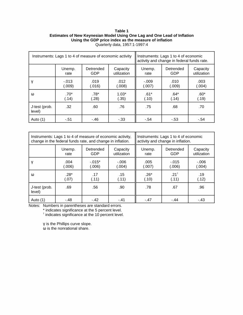
Table 1Estimates of New Keynesian Model Using One Lag and One Lead of Inflation

Using the GDP price index as the measure of inflationQuarterly data, 1957:1-1997:4

Instruments: Lags 1 to 4 of measure of economic activity Instruments: Lags 1 to 4 of economicactivity and change in federal funds rate.

Unemp.rate

DetrendedGDP

Capacityutilization

Unemp.rate

DetrendedGDP

Capacityutilization

� -.013 (.009)

.019(.016)

.012(.008)

-.009(.007)

.010(.009)

.003(.004)

� .70*(.14)

.78*(.28)

1.03*(.35)

.61*(.10)

.64*(.14)

.60*(.19)

J-test (prob.level)

.32 .60 .76 .75 .68 .70

Auto (1) -.51 -.46 -.33 -.54 -.53 -.54

Instruments: Lags 1 to 4 of measure of economic activity,change in the federal funds rate, and change in inflation.

Instruments: Lags 1 to 4 of economicactivity and change in inflation.

Unemp.rate

DetrendedGDP

Capacityutilization

Unemp.rate

DetrendedGDP

Capacityutilization

� .004(.006)

-.015*(.006)

-.006(.004)

.005(.007)

-.015(.006)

-.006(.004)

� .28*(.07)

.17(.11)

.15(.11)

.26*(.10)

.21†

(.11).19

(.12)

J-test (prob.level)

.69 .56 .90 .78 .67 .96

Auto (1) -.48 -.42 -.41 -.47 -.44 -.43Notes: Numbers in parentheses are standard errors.

* indicates significance at the 5 percent level.† indicates significance at the 10 percent level.

� is the Phillips curve slope.� is the nonrational share.

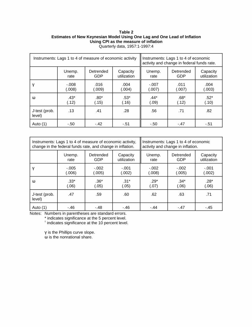
Table 2Estimates of New Keynesian Model Using One Lag and One Lead of Inflation

Using CPI as the measure of inflationQuarterly data, 1957:1-1997:4


Unemp.rate

DetrendedGDP

Capacityutilization

Unemp.rate

DetrendedGDP

Capacityutilization

� -.008(.008)

.016(.009)

.004(.004)

-.007(.007)

.011(.007)

.004(.003)

� .43*(.12)

.80*(.15)

.53*(.16)

.44*(.09)

.68*(.12)

.52*(.10)

J-test (prob.level)

.13 .41 .28 .56 .71 .82

Auto (1) -.50 -.42 -.51 -.50 -.47 -.51



Unemp.rate

DetrendedGDP

Capacityutilization

Unemp.rate

DetrendedGDP

Capacityutilization

� -.005(.006)

-.002(.005)

-.001(.002)

-.002(.008)

-.002(.005)

-.001(.002)

� .33*(.06)

.36*(.05)

.31*(.05)

.29*(.07)

.34*(.06)

.28*(.06)

J-test (prob.level)

.47 .59 .60 .62 .63 .71

Auto (1) -.46 -.48 -.46 -.44 -.47 -.45Notes: Numbers in parentheses are standard errors.



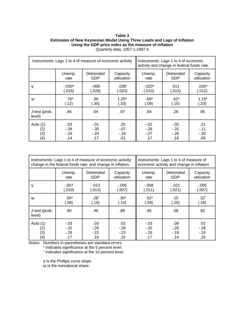
Table 3Estimates of New Keynesian Model Using Three Leads and Lags of Inflation

Using the GDP price index as the measure of inflationQuarterly data, 1957:1-1997:4


Unemp.rate

DetrendedGDP

Capacityutilization

Unemp.rate

DetrendedGDP

Capacityutilization

� -.030*(.015)

-.006(.028)

.038†

(.020)-.020*(.010)

.011(.013)

.026*(.012)

� .76*(.12)

.39(.35)

1.25*(.33)

.69*(.09)

.62*(.15)

1.15*(.23)

J-test (prob.level)

.46 .04 .97 .84 .26 .95

Auto (1) (2) (3) (4)

.03-.26-.24 .14

-.01-.30-.24 .17

.25-.07-.19 .01

-.02-.26-.27 .17

-.02-.31-.26 .16

.21-.11-.20 .05

Instruments: Lags 1 to 4 of measure of economic activity;change in the federal funds rate; and change in inflation.

Instruments: Lags 1 to 4 of measure ofeconomic activity and change in inflation.

Unemp.rate

DetrendedGDP

Capacityutilization

Unemp.rate

DetrendedGDP

Capacityutilization

� -.007(.010)

-.013(.013)

-.006(.007)

-.008(.011)

-.021(.021)

-.005(.007)

� .50*(.08)

.28†

(.16) .30*(.14)

.52*(.09)

.15(.25)

.32†

(.16)

J-test (prob.level)

.80 .46 .89 .85 .58 .92

Auto (1) (2) (3) (4)

-.03-.32-.26 .17

.03-.26-.22 .16

.02-.28-.23 .16

-.03-.32-.26 .17

.09-.20-.19 .14

.01-.28-.24 .16

Notes: Numbers in parentheses are standard errors.* indicates significance at the 5 percent level.† indicates significance at the 10 percent level.


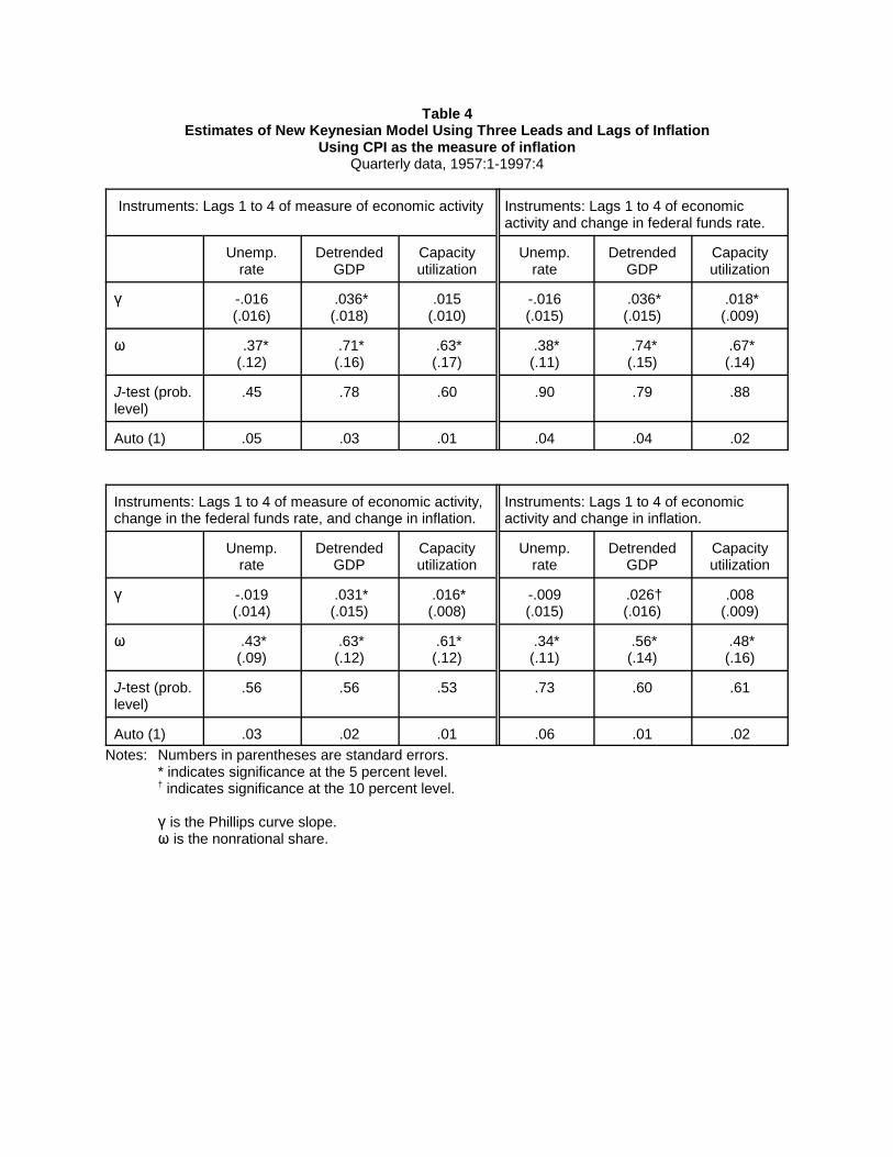
Table 4Estimates of New Keynesian Model Using Three Leads and Lags of Inflation

Using CPI as the measure of inflationQuarterly data, 1957:1-1997:4


Unemp.rate

DetrendedGDP

Capacityutilization

Unemp.rate

DetrendedGDP

Capacityutilization

� -.016(.016)

.036*(.018)

.015(.010)

-.016(.015)

.036*(.015)

.018*(.009)

� .37*(.12)

.71*(.16)

.63*(.17)

.38*(.11)

.74*(.15)

.67*(.14)

J-test (prob.level)

.45 .78 .60 .90 .79 .88

Auto (1) .05 .03 .01 .04 .04 .02



Unemp.rate

DetrendedGDP

Capacityutilization

Unemp.rate

DetrendedGDP

Capacityutilization

� -.019(.014)

.031*(.015)

.016*(.008)

-.009(.015)

.026†(.016)

.008(.009)

� .43*(.09)

.63*(.12)

.61*(.12)

.34*(.11)

.56*(.14)

.48*(.16)

J-test (prob.level)

.56 .56 .53 .73 .60 .61

Auto (1) .03 .02 .01 .06 .01 .02Notes: Numbers in parentheses are standard errors.



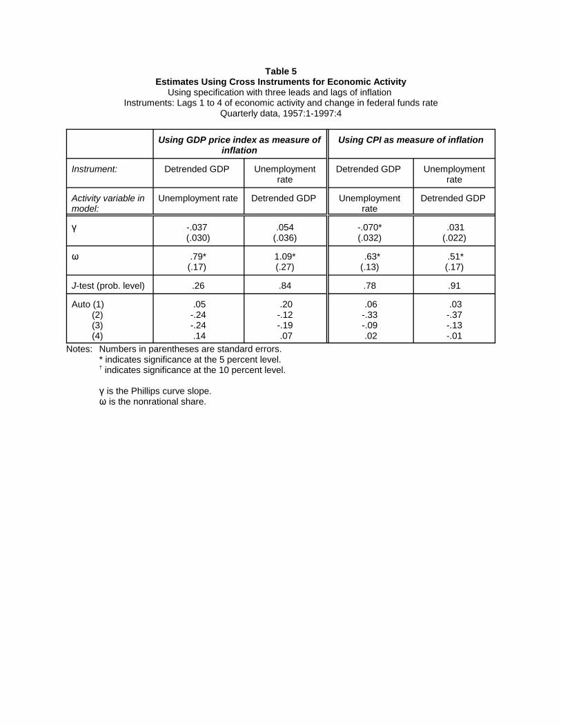
Table 5Estimates Using Cross Instruments for Economic Activity

Using specification with three leads and lags of inflation Instruments: Lags 1 to 4 of economic activity and change in federal funds rate

Quarterly data, 1957:1-1997:4

Using GDP price index as measure ofinflation

Using CPI as measure of inflation

Instrument: Detrended GDP Unemploymentrate

Detrended GDP Unemploymentrate

Activity variable inmodel:

Unemployment rate Detrended GDP Unemploymentrate

Detrended GDP

� -.037 (.030)

.054(.036)

-.070*(.032)

.031(.022)

� .79*(.17)

1.09*(.27)

.63*(.13)

.51*(.17)

J-test (prob. level) .26 .84 .78 .91

Auto (1) (2) (3) (4)

.05-.24-.24 .14

.20-.12-.19 .07

.06-.33-.09 .02

.03-.37-.13-.01



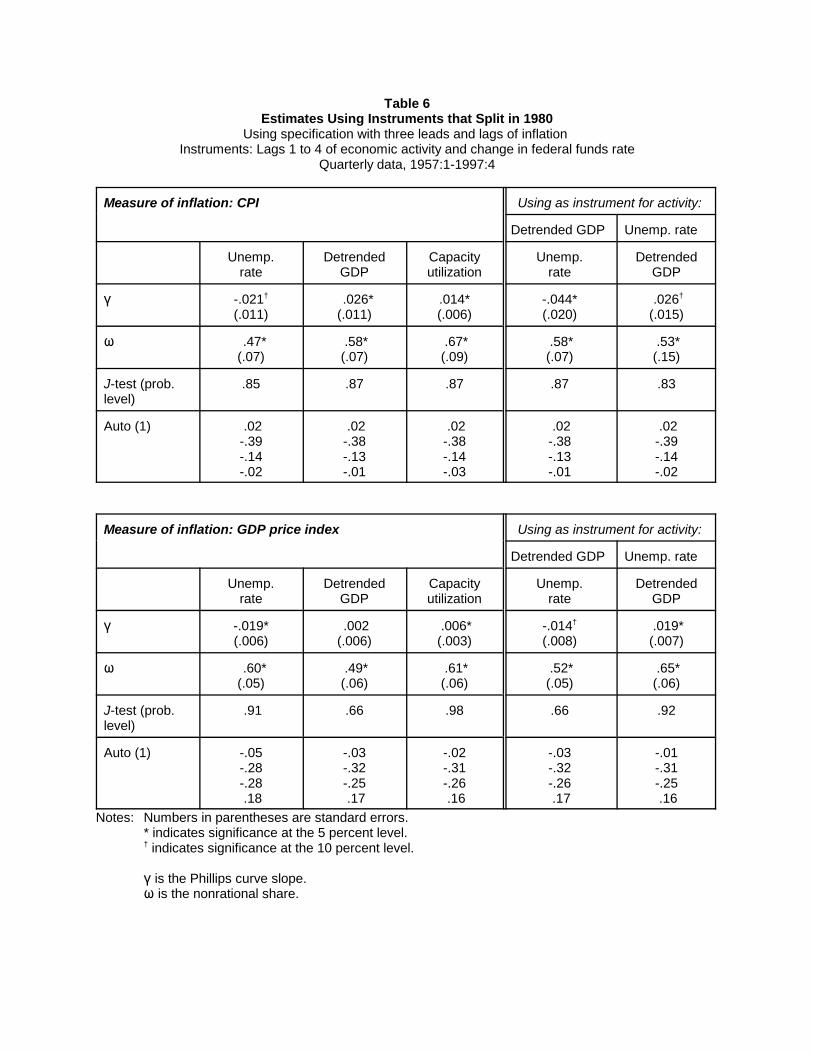
Table 6Estimates Using Instruments that Split in 1980

Using specification with three leads and lags of inflation Instruments: Lags 1 to 4 of economic activity and change in federal funds rate


Measure of inflation: CPI Using as instrument for activity:

Detrended GDP Unemp. rate

Unemp.rate

DetrendedGDP

Capacityutilization

Unemp.rate

DetrendedGDP

� -.021†

(.011) .026*(.011)

.014*(.006)

-.044*(.020)

.026†

(.015)

� .47*(.07)

.58*(.07)

.67*(.09)

.58*(.07)

.53*(.15)

J-test (prob.level)

.85 .87 .87 .87 .83

Auto (1) .02-.39-.14-.02

.02-.38-.13-.01

.02-.38-.14-.03

.02-.38-.13-.01

.02-.39-.14-.02

Measure of inflation: GDP price index Using as instrument for activity:

Detrended GDP Unemp. rate

Unemp.rate

DetrendedGDP

Capacityutilization

Unemp.rate

DetrendedGDP

� -.019*(.006)

.002(.006)

.006*(.003)

-.014†

(.008) .019*(.007)

� .60*(.05)

.49*(.06)

.61*(.06)

.52*(.05)

.65*(.06)

J-test (prob.level)

.91 .66 .98 .66 .92

Auto (1) -.05-.28-.28 .18

-.03-.32-.25 .17

-.02-.31-.26 .16

-.03-.32-.26 .17

-.01-.31-.25 .16



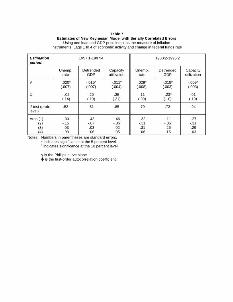
Table 7Estimates of New Keynesian Model with Serially Correlated Errors

Using one lead and GDP price index as the measure of inflationInstruments: Lags 1 to 4 of economic activity and change in federal funds rate

Estimationperiod:

1957:1-1997:4 1980:2-1995:2

Unemp.rate

DetrendedGDP

Capacityutilization

Unemp.rate

DetrendedGDP

Capacityutilization

� .020*(.007)

-.015*(.007)

-.011*(.004)

.029*(.008)

-.018*(.003)

-.009*(.003)

� -.02 (.14)

.20(.19)

.25(.21)

.11(.09)

-.23*(.10)

.01(.19)

J-test (prob.level)

.53 .81 .85 .79 .73 .94

Auto (1) (2) (3) (4)

-.30-.15 .03 .08

-.43-.07 .03 .06

-.46-.06 .02 .05

-.32-.31 .31 .06

-.11-.36 .26 .15

-.27-.31 .29 .03


� is the Phillips curve slope.� is the first-order autocorrelation coefficient.

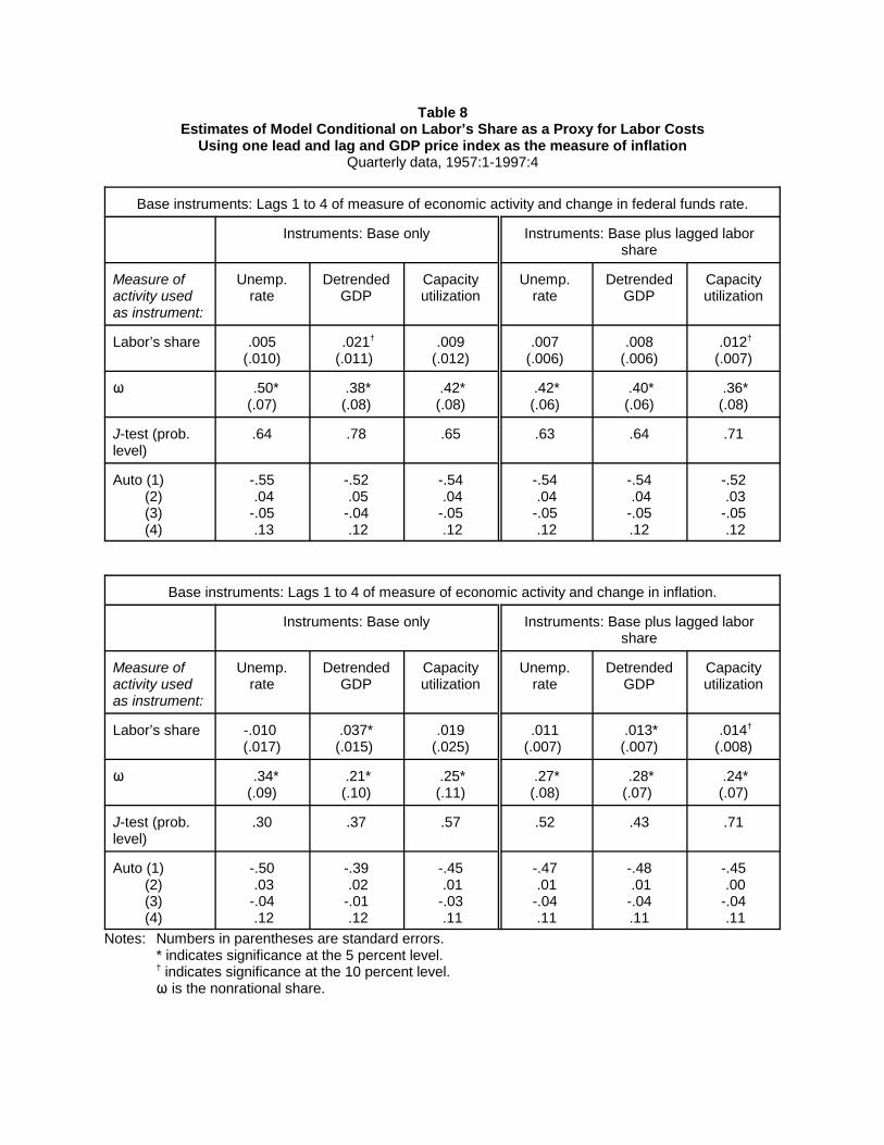
Table 8Estimates of Model Conditional on Labor’s Share as a Proxy for Labor Costs

Using one lead and lag and GDP price index as the measure of inflationQuarterly data, 1957:1-1997:4

Base instruments: Lags 1 to 4 of measure of economic activity and change in federal funds rate.

Instruments: Base only Instruments: Base plus lagged laborshare

Measure ofactivity usedas instrument:

Unemp.rate

DetrendedGDP

Capacityutilization

Unemp.rate

DetrendedGDP

Capacityutilization

Labor’s share .005(.010)

.021†

(.011) .009

(.012).007

(.006).008

(.006) .012†

(.007)

� .50*(.07)

.38*(.08)

.42*(.08)

.42*(.06)

.40*(.06)

.36*(.08)

J-test (prob.level)

.64 .78 .65 .63 .64 .71

Auto (1) (2) (3) (4)

-.55 .04-.05 .13

-.52 .05-.04 .12

-.54 .04-.05 .12

-.54 .04-.05 .12

-.54 .04-.05.12

-.52 .03-.05 .12

Base instruments: Lags 1 to 4 of measure of economic activity and change in inflation.

Instruments: Base only Instruments: Base plus lagged laborshare


Unemp.rate

DetrendedGDP

Capacityutilization

Unemp.rate

DetrendedGDP

Capacityutilization

Labor’s share -.010 (.017)

.037*(.015)

.019(.025)

.011(.007)

.013*(.007)

.014†

(.008)

� .34*(.09)

.21*(.10)

.25*(.11)

.27*(.08)

.28*(.07)

.24*(.07)

J-test (prob.level)

.30 .37 .57 .52 .43 .71

Auto (1) (2) (3) (4)

-.50 .03-.04 .12

-.39 .02-.01 .12

-.45 .01-.03 .11

-.47 .01-.04 .11

-.48 .01-.04.11

-.45 .00-.04 .11

Notes: Numbers in parentheses are standard errors.* indicates significance at the 5 percent level.† indicates significance at the 10 percent level.� is the nonrational share.

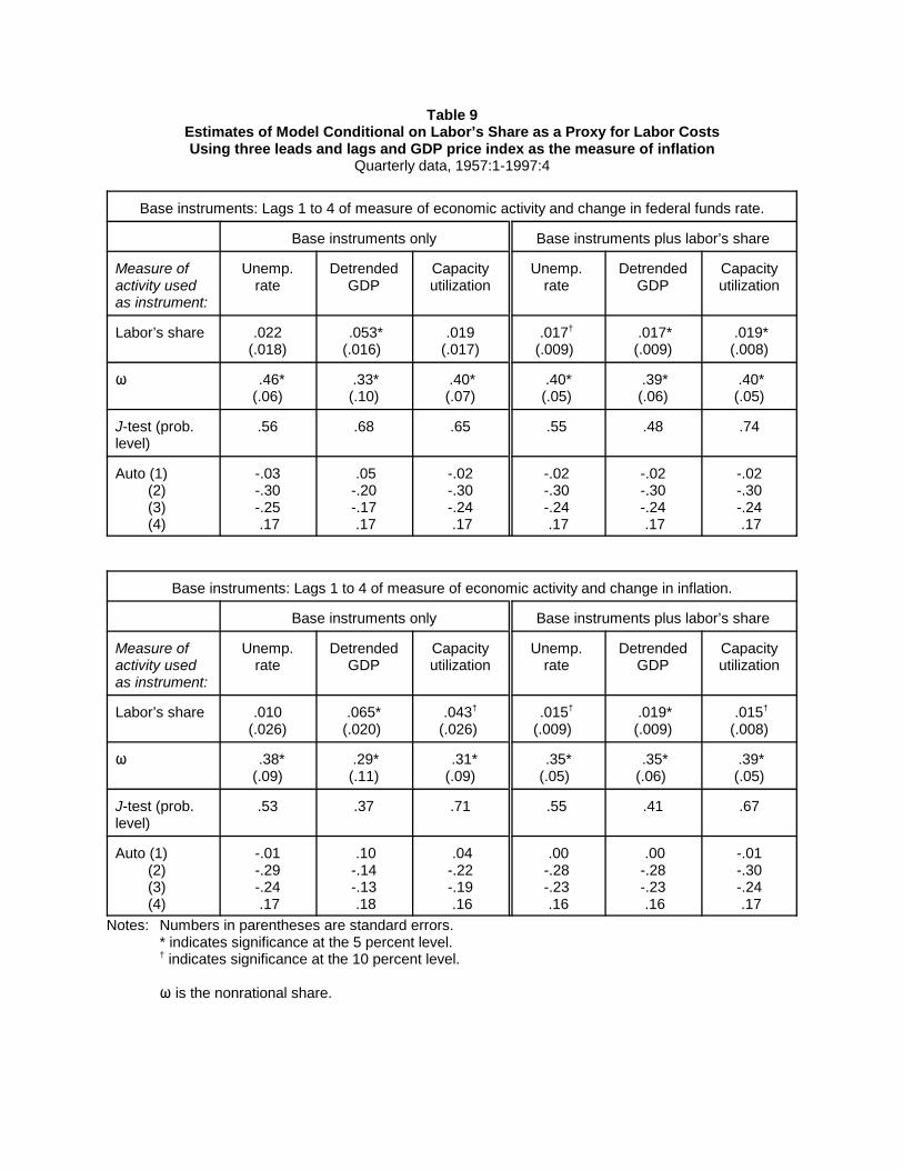
Table 9Estimates of Model Conditional on Labor’s Share as a Proxy for Labor CostsUsing three leads and lags and GDP price index as the measure of inflation



Base instruments only Base instruments plus labor’s share


Unemp.rate

DetrendedGDP

Capacityutilization

Unemp.rate

DetrendedGDP

Capacityutilization


.053*(.016)

.019(.017)

.017†

(.009) .017*(.009)

.019*(.008)

� .46*(.06)

.33*(.10)

.40*(.07)

.40*(.05)

.39*(.06)

.40*(.05)

J-test (prob.level)

.56 .68 .65 .55 .48 .74

Auto (1) (2) (3) (4)

-.03-.30-.25 .17

.05-.20-.17 .17

-.02-.30-.24 .17

-.02-.30-.24 .17

-.02-.30-.24 .17

-.02-.30-.24 .17




Unemp.rate

DetrendedGDP

Capacityutilization

Unemp.rate

DetrendedGDP

Capacityutilization

Labor’s share .010 (.026)

.065*(.020)

.043†

(.026) .015†

(.009) .019*(.009)

.015†

(.008)

� .38*(.09)

.29*(.11)

.31*(.09)

.35*(.05)

.35*(.06)

.39*(.05)

J-test (prob.level)

.53 .37 .71 .55 .41 .67

Auto (1) (2) (3) (4)

-.01-.29-.24 .17

.10-.14-.13 .18

.04-.22-.19 .16

.00-.28-.23 .16

.00-.28-.23 .16

-.01-.30-.24 .17


� is the nonrational share.

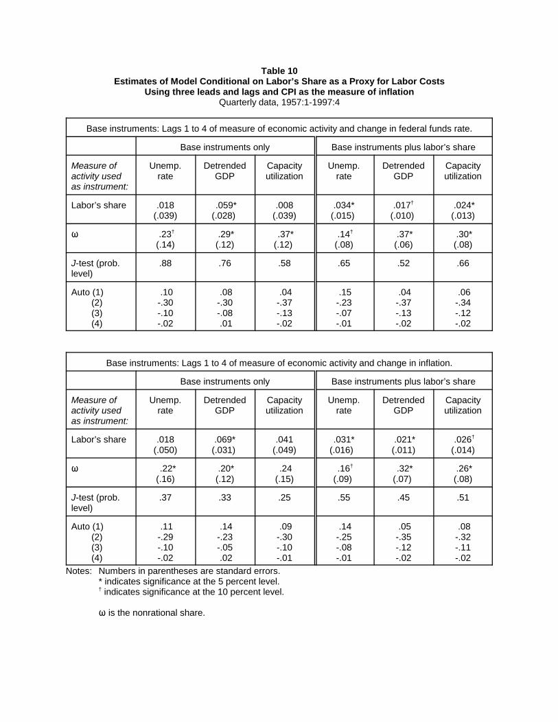
Table 10Estimates of Model Conditional on Labor’s Share as a Proxy for Labor Costs

Using three leads and lags and CPI as the measure of inflationQuarterly data, 1957:1-1997:4




Unemp.rate

DetrendedGDP

Capacityutilization

Unemp.rate

DetrendedGDP

Capacityutilization


.059*(.028)

.008(.039)

.034*(.015)

.017† (.010)

.024*(.013)

� .23†

(.14) .29*(.12)

.37*(.12)

.14†

(.08) .37*(.06)

.30*(.08)

J-test (prob.level)

.88 .76 .58 .65 .52 .66

Auto (1) (2) (3) (4)

.10-.30-.10-.02

.08-.30-.08 .01

.04-.37-.13-.02

.15-.23-.07-.01

.04-.37-.13-.02

.06-.34-.12-.02




Unemp.rate

DetrendedGDP

Capacityutilization

Unemp.rate

DetrendedGDP

Capacityutilization

Labor’s share .018 (.050)

.069*(.031)

.041(.049)

.031*(.016)

.021*(.011)

.026†

(.014)

� .22*(.16)

.20*(.12)

.24(.15)

.16†

(.09) .32*(.07)

.26*(.08)

J-test (prob.level)

.37 .33 .25 .55 .45 .51

Auto (1) (2) (3) (4)

.11-.29-.10-.02

.14-.23-.05 .02

.09-.30-.10-.01

.14-.25-.08-.01

.05-.35-.12-.02

.08-.32-.11-.02


� is the nonrational share.

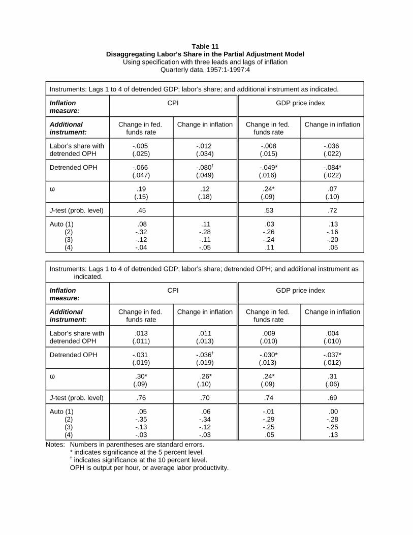
Table 11Disaggregating Labor’s Share in the Partial Adjustment Model

Using specification with three leads and lags of inflationQuarterly data, 1957:1-1997:4

Instruments: Lags 1 to 4 of detrended GDP; labor’s share; and additional instrument as indicated.

Inflationmeasure:

CPI GDP price index

Additionalinstrument:

Change in fed. funds rate

Change in inflation Change in fed. funds rate

Change in inflation

Labor’s share withdetrended OPH

-.005 (.025)

-.012 (.034)

-.008(.015)

-.036 (.022)

Detrended OPH -.066 (.047)

-.080†

(.049)-.049*(.016)

-.084*(.022)

� .19(.15)

.12(.18)

.24*(.09)

.07(.10)

J-test (prob. level) .45 .53 .72

Auto (1) (2) (3) (4)

.08-.32-.12-.04

.11-.28-.11-.05

.03-.26-.24 .11

.13-.16-.20 .05

Instruments: Lags 1 to 4 of detrended GDP; labor’s share; detrended OPH; and additional instrument asindicated.

Inflationmeasure:

CPI GDP price index

Additionalinstrument:

Change in fed. funds rate

Change in inflation Change in fed. funds rate

Change in inflation

Labor’s share withdetrended OPH

.013 (.011)

.011 (.013)

.009(.010)

.004(.010)


-.036†

(.019)-.030*(.013)

-.037*(.012)

� .30*(.09)

.26*(.10)

.24*(.09)

.31(.06)

J-test (prob. level) .76 .70 .74 .69

Auto (1) (2) (3) (4)

.05-.35-.13-.03

.06-.34-.12-.03

-.01-.29-.25 .05

.00-.28-.25 .13

Notes: Numbers in parentheses are standard errors.* indicates significance at the 5 percent level.† indicates significance at the 10 percent level.OPH is output per hour, or average labor productivity.

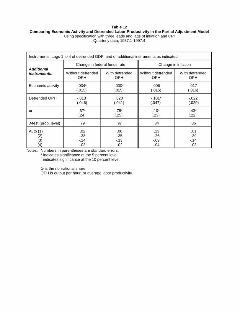
Table 12Comparing Economic Activity and Detrended Labor Productivity in the Partial Adjustment Model

Using specification with three leads and lags of inflation and CPIQuarterly data, 1957:1-1997:4

Instruments: Lags 1 to 4 of detrended GDP; and of additional instruments as indicated.

Additionalinstruments:

Change in federal funds rate Change in inflation

Without detrendedOPH

With detrendedOPH

Without detrendedOPH

With detrendedOPH

Economic activity .034*(.015)

.030*(.015)

.006(.015)

.017(.016)


.028(.041)

-.101*(.047)

-.022 (.029)

� .67*(.24)

.78*(.25)

.10*(.23)

.43*(.22)

J-test (prob. level) .79 .97 .34 .86

Auto (1) (2) (3) (4)

.02-.38-.14-.03

.06-.35-.13-.02

.13-.26-.09-.04

.01-.39-.14-.03


� is the nonrational share.OPH is output per hour, or average labor productivity.

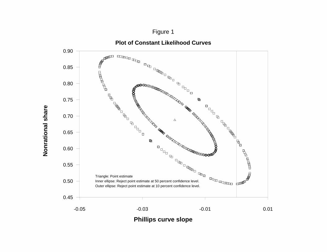
Figure 1

Plot of Constant Likelihood Curves

Phillips curve slope

No

nra

tio

nal

sh

are

-0.05 -0.03 -0.01 0.01

0.45

0.50

0.55

0.60

0.65

0.70

0.75

0.80

0.85

0.90

Triangle: Point estimateInner ellipse: Reject point estimate at 50 percent confidence level.Outer ellipse: Reject point estimate at 10 percent confidence level.

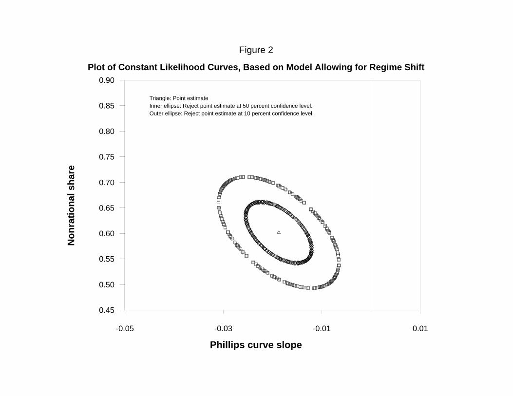
Figure 2

Plot of Constant Likelihood Curves, Based on Model Allowing for Regime Shift

Phillips curve slope

No

nra

tio

nal

sh

are

-0.05 -0.03 -0.01 0.01

0.45

0.50

0.55

0.60

0.65

0.70

0.75

0.80

0.85

0.90

Triangle: Point estimateInner ellipse: Reject point estimate at 50 percent confidence level.Outer ellipse: Reject point estimate at 10 percent confidence level.

-27-

References

Ball, Laurence, and David Romer (1990) “Real Rigidities and the Nonneutrality of Money,”

Review of Economic Studies 57, 183-203.

Brayton, Flint, Andrew Levin, Ralph Tryon, and John C. Williams (1997) “The Evolution of

Macro Models at the Federal Reserve Board,” Carnegie-Rochester Conference Series on

Public Policy 47, 43-81.

Buiter, Willem, and Ian Jewitt (1981) “Staggered Wage Setting with Real Wage Relativities:

Variations on a Theme of Taylor,” The Manchester School 49, 211-28.

Calvo, Guillermo A. (1983) “Staggered Contracts in a Utility-Maximizing Framework,” Journal

of Monetary Economics 12, 383-98.

Chadha, Bankim, Paul R. Masson, and Guy Meredith (1992) “Models of Inflation and the Costs

of Disinflation,” IMF Staff Papers 39, 395-431.

Clarida, Richard, Jordi Gali, and Mark Gertler (1998) “Monetary Policy Rules in Practice: Some

International Evidence,” European Economic Review 42, 1033-67.

Dotsey, Michael, Robert G. King, and Alexander L. Wolman (1999) “State-Dependent Pricing

and the General Equilibrium Dynamics of Money and Output,” Quarterly Journal of

Economics 114, 655-90.

Fuhrer, Jeffrey (1997a) “Inflation/Output Variance Trade-offs and Optimal Monetary Policy,”

Journal of Money, Credit, and Banking 29, 214-34.

_________ (1997b) “The (Un)Importance of Forward-Looking Behavior in Price Specifications,”

Journal of Money, Credit, and Banking 29, 338-50.

_________ and George R. Moore (1995) “Inflation Persistence,” Quarterly Journal of Economics

110, 127-59.

Gali, Jordi and Mark Gertler (1999) “Inflation Dynamics: A Structural Econometric Analysis,”

Journal of Monetary Economics 44, 195-222.

King, Robert G., and Alexander L. Wolman (1999) “What Should the Monetary Authority Do

When Prices Are Sticky?” in John B. Taylor, ed., Monetary Policy Rules, University of

Chicago Press, 349-404.

Levin, Andrew, Volker Wieland, and John C. Williams (1999) “Robustness of Simple Monetary

Policy Rules under Model Uncertainty,” in John B. Taylor, ed., Monetary Policy Rules,

University of Chicago Press, 263-318.

-28-

Lucas, Robert E. (1967) “Adjustment Costs and the Theory of Supply,” Journal of Political

Economy 75, 321-34.

Roberts, John M. (1992) “Evidence on Price Adjustment Costs in U.S. Manufacturing Industry,”

Economic Inquiry 30, 399-417.

_________ (1995) “New Keynesian Economics and the Phillips Curve,” Journal of Money,

Credit, and Banking 27, 975-84.

_________ (1997) “Is Inflation Sticky?” Journal of Monetary Economics 39, 173-96.

_________ (1998) “Inflation Expectations and the Transmission of Monetary Policy,” Federal

Reserve Board FEDS working paper no. 1998-43 (October).

_________, David J. Stockton, and Charles S. Struckmeyer (1994) “Evidence on the Flexibility

of Prices,” Review of Economics and Statistics 76, 142-50.

Rotemberg, Julio J. (1982) “Sticky Prices in the United States,” Journal of Political Economy 60,

1187-1211.

_________ (1987) “The New Keynesian Microfoundations,” in Stanley Fischer, ed., NBER

Macroeconomics Annual 1987, MIT Press, 69-104.

_________ and Michael Woodford (1997) “An Optimization-Based Econometric Framework for

the Evaluation of Monetary Policy,” in Ben S. Bernanke and Julio J. Rotemberg, eds.,

NBER Macroeconomics Annual 1997, MIT Press.

_________ and _________ (1999) “Interest Rate Rules in an Estimated Sticky Price Model,” in

John B. Taylor, ed., Monetary Policy Rules, University of Chicago Press, 57-126.

Rudebusch, Glenn D. (2000) “Assessing Nominal Income Rules for Monetary Policy with Model

and Data Uncertainty,” working paper, www.sf.frb.org/econrsrch/economists/

grudebusch.html

Sbordone, Argia M. (1998) “Prices and Unit Labor Costs: A New Test of Price Stickiness,”

working paper, Rutgers University (October).

Taylor, John B., (1999), ed., Monetary Policy Rules, University of Chicago Press.

How Well Does the New Keynesian Sticky-Price … Well Does the New Keynesian Sticky-Price Model Fit...

Documents

Transcript of How Well Does the New Keynesian Sticky-Price … Well Does the New Keynesian Sticky-Price Model Fit...