How to Explain Individual Classiﬁcation...

Journal of Machine Learning Research 11 (2010) 1803-1831 Submitted 4/09; Revised 11/09; Published 6/10

How to Explain Individual Classification Decisions

David Baehrens∗ [email protected]

Timon Schroeter∗ [email protected]

Technische Universitat BerlinFranklinstr. 28/29, FR 6-910587 Berlin, Germany

Stefan Harmeling∗ [email protected]

MPI for Biological CyberneticsSpemannstr. 3872076 Tubingen, Germany

Motoaki Kawanabe† MOTOAKI .KAWANABE @FIRST.FRAUNHOFER.DE

Fraunhofer Institute FIRST.IDAKekulestr.712489 Berlin, Germany

Katja Hansen [email protected]

Klaus-Robert Muller [email protected]

Technische Universitat BerlinFranklinstr. 28/29, FR 6-910587 Berlin, Germany

Editor: Carl Edward Rasmussen

AbstractAfter building a classifier with modern tools of machine learning we typically have a black box athand that is able to predict well for unseen data. Thus, we getan answer to the questionwhat is themost likely label of a given unseen data point. However, mostmethods will provide no answerwhythe model predicted a particular label for a single instanceand what features were most influentialfor that particular instance. The only method that is currently able to provide such explanations aredecision trees. This paper proposes a procedure which (based on a set of assumptions) allows toexplain the decisions ofanyclassification method.

Keywords: explaining, nonlinear, black box model, kernel methods, Ames mutagenicity

1. Introduction

Automatic nonlinear classification is a common and powerful tool in data analysis. Machine learn-ing research has created methods that are practically useful and that can classify unseen data afterbeing trained on a limited training set of labeled examples.

Nevertheless, most of the algorithms do notexplain their decision. However in practical dataanalysis it is essential to obtain an instance-based explanation, that is, we would like to gain an

∗. The first three authors contributed equally.†. Also at Technische Universitat Berlin, Franklinstr. 28/29, FR 6-9, 10587 Berlin, Germany.

c©2010 David Baehrens, Timon Schroeter, Stefan Harmeling, Motoaki Kawanabe, Katja Hansen and Klaus-Robert Muller.

BAEHRENS, SCHROETER, HARMELING , KAWANABE , HANSEN AND M ULLER

understanding what input features made the nonlinear machine give its answer for each individualdata point.

Typically, explanations are provided jointly for all instances of the training set, for examplefeature selection methods (including Automatic Relevance Determination) find outwhich inputsare salient for a good generalization (see Guyon and Elisseeff, 2003,for a review). While this cangive a coarse impression about the global usefulness of each input dimension, it is still an ensembleview and does not provide an answer on an instance basis.1 In the neural network literature alsosolely an ensemble view was taken in algorithms like input pruning (e.g., Bishop,1995; LeCunet al., 1998). The only classification that does provide individual explanations are decision trees(e.g., Hastie et al., 2001).

This paper proposes a simple framework that provides local explanation vectors applicable toanyclassification method in order to help understanding prediction results for single data instances.The local explanation yields the features relevant for the prediction at thevery points of interestin the data space, and is able to spot local peculiarities that are neglected in the global view, forexample, due to cancellation effects.

The paper is organized as follows: We define local explanation vectors as class probability gradi-ents in Section 2 and give an illustration for Gaussian Process Classification(GPC). Some methodsoutput a prediction without a direct probability interpretation. For these we propose in Section 3 away to estimate local explanations. In Section 4 we apply our methodology to learn distinguishingproperties of Iris flowers by estimating explanation vectors for a k-NN classifier applied to the clas-sic Iris data set. In Section 5 we discuss how our approach applied to a SVMclassifier allows us toexplain how digit “2” is distinguished from digit “8” in the USPS data set. In Section 6 we focus ona more real-world application scenario where the proposed explanation capabilities prove useful indrug discovery: Human experts regularly decide how to modify existing leadcompounds in orderto obtain new compounds with improved properties. Models capable of explaining predictions canhelp in the process of choosing promising modifications. Our automatically generated explanationsmatch with chemical domain knowledge about toxifying functional groups of the compounds inquestion. Section 7 contrasts our approach with related work and Section 8discusses characteristicproperties and limitations of our approach, before we conclude the paperin Section 9.

2. Definitions of Explanation Vectors

In this Section we will give definitions for our approach of local explanation vectors in the classi-fication setting. We start with a theoretical definition for multi-class Bayes classification and thengive a specialized definition being more practical for the binary case.

For the multi-class case, suppose we are given data pointsx1, . . . ,xn ∈ℜd with labelsy1, . . . ,yn ∈{1, . . . ,C} and we intend to learn a function that predicts the labels of unlabeled data points. As-suming that the data is IID-sampled from some unknown joint distributionP(X,Y), we define the

1. This point is illustrated in Figure 1 (Section 2). Applying feature selection methods to the training set (a) will leadto the (correct) conclusion that both dimensions are equally important foraccurate classification. As an alternativeto this ensemble view, one may ask: Which features (or combinations thereof) are most influential in the vicinityof each particular instance. As can be seen in Figure 1 (c), the answer depends on where the respective instance islocated. On the hypotenuse and at the corners of the triangle, both features contribute jointly, whereas along each ofthe remaining two edges the classification depends almost completely on justone of the features.

1804

HOW TO EXPLAIN INDIVIDUAL CLASSIFICATION DECISIONS

Bayes classifier,

g∗(x) = arg minc∈{1,...,C}

P(Y 6=c | X=x)

which is optimal for the 0-1 loss function (see Devroye et al., 1996).For the Bayes classifier we define theexplanation vectorof a data pointx0 to be the derivative

with respect tox atx= x0 of the conditional probability ofY 6=g∗(x0) givenX = x, or formally,

Definition 1

ζ(x0) :=∂∂x

P(Y 6=g∗(x) | X=x)

∣

∣

∣

∣

x=x0

.

Note thatζ(x0) is ad-dimensional vector just likex0 is. The classifierg∗ partitions the data spaceℜd

into up toC parts on whichg∗ is constant. We assume that the conditional distributionP(Y = c |X =x) is first-order differentiable w.r.t.x for all classesc and over the entire input space. For instance,this assumption holds ifP(X=x | Y=c) is for all c first-order differentiable inx and the supportsof the class densities overlap around the border for all neighboring pairs in the partition by theBayes classifier. The vectorζ(x0) defines on each of those parts a vector field that characterizes theflow away from the corresponding class. Thus entries inζ(x0) with large absolute values highlightfeatures that will influence the class label decision ofx0. A positive sign of such an entry impliesthat increasing that feature would lower the probability thatx0 is assigned tog∗(x0). Ignoring theorientations of the explanation vectors,ζ forms a continuously changing (orientation-less) vectorfield along which the class labels change. This vector field lets uslocally understand the Bayesclassifier.

We remark thatζ(x0) becomes a zero vector, for example, whenP(Y 6=g∗(x) | X = x)|x=x0 isequal to one in some neighborhood ofx0. Our explanation vector fits well to classifiers where theconditional distributionP(Y = c | X = x) is usually not completely flat in some regions. In thecase of deterministic classifiers, despite of this issue, Parzen window estimators with appropriatewidths (Section 3) can provide meaningful explanation vectors for many samples in practice (seealso Section 8).

In the case of binary classification we directly define local explanation vectors as local gradientsof the probability functionp(x) = P(Y = 1 | X = x) of the learned model for the positive class.

For a probability functionp : ℜd → [0,1] of a classification model learned from examples{(x1,y1), . . . ,(xn,yn)} ∈ ℜd ×{−1,+1} the explanation vector for a classified test pointx0 is thelocal gradient ofp atx0:

Definition 2ηp(x0) := ∇p(x)|x=x0.

By this definition the explanationη is again ad-dimensional vector just like the test pointx0 is.The sign of each of its individual entries indicates whether the prediction would increase or decreasewhen the corresponding feature ofx0 is increased locally and each entry’s absolute value gives theamount of influence in the change in prediction. The vectorη gives the direction of the steepestascent from the test point to higher probabilities for the positive class. For binary classification thenegative version−ηp(x0) indicates the changes in features needed to increase the probability forthe negative class which may be especially useful forx0 predicted in the positive class.

1805


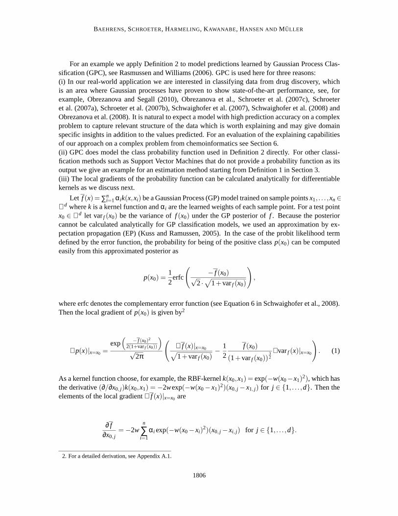
For an example we apply Definition 2 to model predictions learned by GaussianProcess Clas-sification (GPC), see Rasmussen and Williams (2006). GPC is used here forthree reasons:(i) In our real-world application we are interested in classifying data from drug discovery, whichis an area where Gaussian processes have proven to show state-of-the-art performance, see, forexample, Obrezanova and Segall (2010), Obrezanova et al., Schroeter et al. (2007c), Schroeteret al. (2007a), Schroeter et al. (2007b), Schwaighofer et al. (2007), Schwaighofer et al. (2008) andObrezanova et al. (2008). It is natural to expect a model with high prediction accuracy on a complexproblem to capture relevant structure of the data which is worth explaining and may give domainspecific insights in addition to the values predicted. For an evaluation of the explaining capabilitiesof our approach on a complex problem from chemoinformatics see Section 6.(ii) GPC does model the class probability function used in Definition 2 directly. For other classi-fication methods such as Support Vector Machines that do not provide a probability function as itsoutput we give an example for an estimation method starting from Definition 1 in Section 3.(iii) The local gradients of the probability function can be calculated analytically for differentiablekernels as we discuss next.

Let f (x)=∑ni=1 αik(x,xi) be a Gaussian Process (GP) model trained on sample pointsx1, . . . ,xn∈

ℜd wherek is a kernel function andαi are the learned weights of each sample point. For a test pointx0 ∈ ℜd let varf (x0) be the variance off (x0) under the GP posterior off . Because the posteriorcannot be calculated analytically for GP classification models, we used an approximation by ex-pectation propagation (EP) (Kuss and Ramussen, 2005). In the case ofthe probit likelihood termdefined by the error function, the probability for being of the positive class p(x0) can be computedeasily from this approximated posterior as

p(x0) =12

erfc

(

− f (x0)√2 ·√

1+varf (x0)

)

,

where erfc denotes the complementary error function (see Equation 6 in Schwaighofer et al., 2008).Then the local gradient ofp(x0) is given by2

∇p(x)|x=x0 =exp(

− f (x0)2

2(1+varf (x0))

)

√2π

(

∇ f (x)|x=x0√

1+varf (x0)− 1

2f (x0)

(1+varf (x0))32

∇varf (x)|x=x0

)

. (1)

As a kernel function choose, for example, the RBF-kernelk(x0,x1) = exp(−w(x0−x1)2), which has

the derivative(∂/∂x0, j)k(x0,x1) =−2wexp(−w(x0−x1)2)(x0, j −x1, j) for j ∈ {1, . . . ,d}. Then the

elements of the local gradient∇ f (x)|x=x0 are

∂ f∂x0, j

=−2wn

∑i=1

αi exp(−w(x0−xi)2)(x0, j −xi, j) for j ∈ {1, . . . ,d}.

2. For a detailed derivation, see Appendix A.1.

1806


For varf (x0) = k(x0,x0)−kT∗ (K+Σ)−1k∗ the derivative is given by3

∇varf (x)|x=x0 =∂varf

∂x0, j=

(

∂∂x0, j

k(x0,x0)

)

−2∗kT∗ (K+Σ)−1 ∂

∂x0, jk∗ for j ∈ {1, . . . ,d}.

0

0.2

0.4

0.6

0.8

1 00.2

0.40.6

0.81

−1

−0.5

0

0.5

1

(a) Object

0

0.2

0.4

0.6

0.8

1 00.2

0.40.6

0.81

0

0.2

0.4

0.6

0.8

1

(b) Model

0

0.2

0.4

0.6

0.8

1 0

0.1

0.2

0.3

0.4

0.5

0.6

0.7

0.8

0.9

1

(c) Local explanation vectors

0

0.2

0.4

0.6

0.8

1 0

0.1

0.2

0.3

0.4

0.5

0.6

0.7

0.8

0.9

1

(d) Direction of explanation vectors

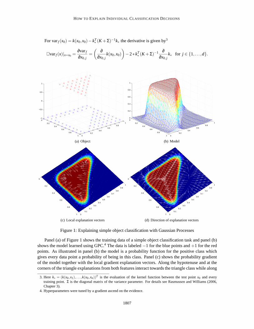
Figure 1: Explaining simple object classification with Gaussian Processes

Panel (a) of Figure 1 shows the training data of a simple object classificationtask and panel (b)shows the model learned using GPC.4 The data is labeled−1 for the blue points and+1 for the redpoints. As illustrated in panel (b) the model is a probability function for the positive class whichgives every data point a probability of being in this class. Panel (c) shows the probability gradientof the model together with the local gradient explanation vectors. Along the hypotenuse and at thecorners of the triangle explanations from both features interact towardsthe triangle class while along

3. Herek∗ = (k(x0,x1), . . . ,k(x0,xn))T is the evaluation of the kernel function between the test pointx0 and every

training point. Σ is the diagonal matrix of the variance parameter. For details see Rasmussen and Williams (2006,Chapter 3).

4. Hyperparameters were tuned by a gradient ascend on the evidence.

1807


the edges the importance of one of the two feature dimensions dominates. At thetransition fromthe negative to the positive class the length of the local gradient vectors represents the increasedimportance of the relevant features. In panel (d) we see that explanations close to the edges of theplot (especially in the right hand side corner) point away from the positive class. However, panel(c) shows that their magnitude is very small. For discussion of this issue see Section 8.

3. Estimating Explanation Vectors

Several classification methods directly estimate the decision rule, which often has no interpretationas the probability function in terms of Definition 2. For example Support VectorMachines estimatea decision function of the form

f (x) =n

∑i=1

αik(xi ,x)+b,

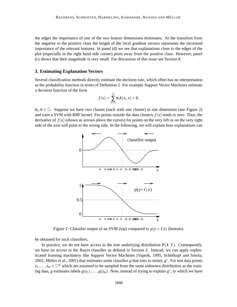
αi ,b ∈ ℜ. Suppose we have two classes (each with one cluster) in one dimension (see Figure 2)and train a SVM with RBF kernel. For points outside the data clustersf (x) tends to zero. Thus, thederivative of f (x) (shown as arrows above the curves) for points on the very left or on the very rightside of the axis will point to the wrong side. In the following, we will explain howexplanations can

0

x

p( | )y=1 x1

0.5

0

x

classifier output

Figure 2: Classifier output of an SVM (top) compared top(y=1|x) (bottom).

be obtained for such classifiers.In practice, we do not have access to the true underlying distributionP(X,Y). Consequently,

we have no access to the Bayes classifier as defined in Section 2. Instead, we can apply sophis-ticated learning machinery like Support Vector Machines (Vapnik, 1995; Scholkopf and Smola,2002; Muller et al., 2001) that estimates some classifierg that tries to mimicg∗. For test data pointsz1, . . . ,zm ∈ ℜd which are assumed to be sampled from the same unknown distribution as the train-ing data,g estimates labelsg(z1), . . . ,g(zm). Now, instead of trying to explaing∗, to which we have

1808


no access, we will define explanation vectors that help us understand theclassifierg on the test datapoints.

Since we do not assume that we have access to some intermediate real-valuedclassifier outputhere (of whichg might be a thresholded version and which further might not be an estimate ofP(Y=c | X=x)), we suggest to approximateg by another classifier ˆg, the actual form of which resemblesthe Bayes classifier. There are several choices for ˆg, for example, GPC, logistic regression, andParzen windows.5 In this paper we apply Parzen windows to the training points to estimate theweighted class densitiesP(Y=c) ·P(X |Y=c), for the index setIc = {i | g(xi) = c}

pσ(x,y=c) =1n ∑

i∈Ic

kσ(x−xi) (2)

and withkσ(z) being a Gaussian kernelkσ(z) = exp(−0.5 z⊤z/σ2)/√

2πσ2 (as always other kernelsare also possible). This estimatesP(Y=c | X=x) for all c,

pσ(y=c|x) = pσ(x,y=c)pσ(x,y=c)+ pσ(x,y 6=c)

≈ ∑i∈Ic kσ(x−xi)

∑i kσ(x−xi)(3)

and thus is an estimate of the Bayes classifier (that mimicsg),

gσ(x) = arg minc∈{1,...,C}

pσ(y 6=c | x).

This approach has the advantage that we can use our estimated classifierg to generate any amountof labeled data for constructing ˆg. The single hyper-parameterσ is chosen such that ˆg approximatesg (which we want to explain), that is,

σ := argminσ

m

∑j=1

I{

g(zj) 6= gσ(zj)}

,

whereI{· · ·} is the indicator function.σ is assigned the constant valueσ from here on and omittedas a subscript. For ˆg it is straightforward to define explanation vectors:

Definition 3

ζ(z) :=∂∂x

p(y 6=g(z) | x)

∣

∣

∣

∣

x=z=

(

∑i /∈Ig(z) k(z−xi))(

∑i∈Ig(z) k(z−xi)(z−xi))

σ2(

∑ni=1k(z−xi)

)2

−

(

∑i /∈Ig(z) k(z−xi)(z−xi))(

∑i∈Ig(z) k(z−xi))

σ2(

∑ni=1k(z−xi)

)2 .

This is easily derived using Equation (3) and the derivative of Equation (2), see Appendix A.3.1.Note that we useg instead of ˆg. This choice ensures that the orientation ofζ(z) fits to the labelsassigned byg, which allows better interpretations.

In summary, we imitate the classifierg which we would like to explain locally by a Parzenwindow classifier ˆg that has the same form as the Bayes estimator and for which we can estimate the

5. For Support Vector Machines Platt (1999) fits a sigmoid function to mapthe outputs to probabilities. In the following,we will present a more general method for estimating explanation vectors.

1809


explanation vectors using Definition 3. Practically there are some caveats: The mimicking classifierg has to be estimated fromg even in high dimensions; this needs to be done with care. However,in principle we have an arbitrary amount of training data available for constructing g since we mayuse our estimated classifierg to generate labeled data.

4. Explaining Iris Flower Classification by k-Nearest Neighbors

The Iris flower data set (introduced in Fisher, 1936) describes 150 flowers from the genus Iris by fourfeatures: sepal length, sepal width, petal length, and petal width, all ofwhich are easily measuredproperties of certain leaves of the corolla of the flower. There are threeclusters in this data set thatcorrespond to three different species:Iris setosa, Iris virginica, andIris versicolor.

Let us consider the problem of classifying the data points ofIris versicolor (class 0) against theother two species (class 1). We applied standard classification machinery tothis problem as follows:

• Class 0 consists of all examples ofIris versicolor.

• Class 1 consists of all examples ofIris setosaandIris virginica.

• Randomly split 150 data points into 100 training and 50 test examples.

• Normalize training and test set using the mean and variance of the training set.

• Apply k-nearest neighbor classification withk= 4 (chosen by leave-one-out cross-validationon the training data).

• Training error is 3% (i.e., 3 mistakes in 100).

• Test error is 8% (i.e., 4 mistakes in 50).

In order to estimate explanation vectors we mimic the classification results with a Parzen windowclassifier. The best fit (3% error) is obtained with a kernel width ofσ = 0.26 (chosen by leave-one-out cross-validation on the training data).

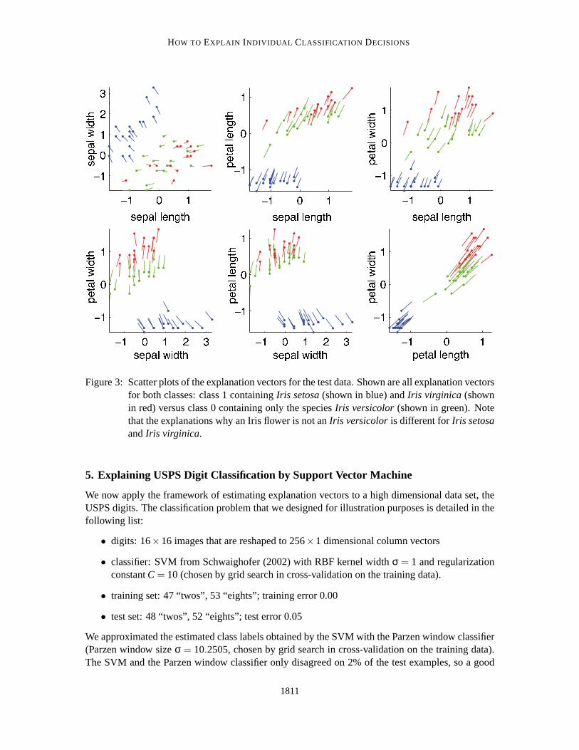
Since the explanation vectors live in the input space we can visualize them withscatter plots ofthe initially measured features. The resultingexplanations(i.e., vectors) for the test set are shownin Figure 3. The blue markers correspond to explanation vectors ofIris setosaand the red markerscorrespond to those of ofIris virginica (both class 1). Both groups of markers point to the greenmarkers ofIris versicolor. The most important feature is the combination of petal length and petalwidth (see the corresponding panel), the product of which corresponds roughly to the area of thepetals. However, the resulting explanations for the two species in class 1 are different:

• Iris setosa(class 1) is different fromIris versicolor(class 0) because its petal area issmaller.

• Iris virginica (class 1) is different fromIris versicolor(class 0) because its petal area islarger.

Also the dimensions of the sepal (another part of the blossom) are relevant, but not as distinguishing.

1810


Figure 3: Scatter plots of the explanation vectors for the test data. Shown are all explanation vectorsfor both classes: class 1 containingIris setosa(shown in blue) andIris virginica (shownin red) versus class 0 containing only the speciesIris versicolor (shown in green). Notethat the explanations why an Iris flower is not anIris versicolor is different forIris setosaandIris virginica.

5. Explaining USPS Digit Classification by Support Vector Machine

We now apply the framework of estimating explanation vectors to a high dimensional data set, theUSPS digits. The classification problem that we designed for illustration purposes is detailed in thefollowing list:

• digits: 16×16 images that are reshaped to 256×1 dimensional column vectors

• classifier: SVM from Schwaighofer (2002) with RBF kernel widthσ = 1 and regularizationconstantC= 10 (chosen by grid search in cross-validation on the training data).

• training set: 47 “twos”, 53 “eights”; training error 0.00

• test set: 48 “twos”, 52 “eights”; test error 0.05

We approximated the estimated class labels obtained by the SVM with the Parzen window classifier(Parzen window sizeσ = 10.2505, chosen by grid search in cross-validation on the training data).The SVM and the Parzen window classifier only disagreed on 2% of the testexamples, so a good

1811


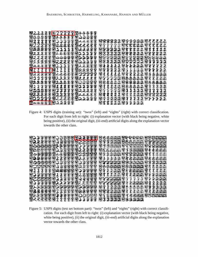
Figure 4: USPS digits (training set): “twos” (left) and “eights” (right) with correct classification.For each digit from left to right: (i) explanation vector (with black being negative, whitebeing positive), (ii) the original digit, (iii-end) artificial digits along the explanation vectortowards the other class.

Figure 5: USPS digits (test set bottom part): “twos” (left) and “eights” (right) with correct classifi-cation. For each digit from left to right: (i) explanation vector (with black being negative,white being positive), (ii) the original digit, (iii-end) artificial digits along the explanationvector towards the other class.

1812


fit was achieved. Figures 4 and 5 show our results. All parts show threeexamples per row. Foreach example we display from left to right: (i) the explanation vector, (ii) the original digit, (iii-end)artificial digits along the explanation vector towards the other class.6 These artificial digits shouldhelp to understand and interpret the explanation vector. Let us first have a look at the results on thetraining set:

Figure 4 (left panel): Let us focus on the top example framed in red. The line that forms the “two”is part of some “eight” from the data set. Thus the parts of the lines that are missing showup in the explanation vector: if the dark parts (which correspond to the missing lines) areadded to the “two” digit then it will be classified as an “eight”. In other words, because ofthe lack of those parts the digit was classified as a “two” and not as an “eight”. A similarexplanation holds for the middle example framed in red in the same Figure. Not allexamplestransform easily to “eights”: Besides adding parts of black lines, some existing black spots(that make the digit be a “two”) must be removed. This is reflected in the explanation vectorby white spots/lines. The bottom “two”, framed in red, is actually a dash and is inthe data setby mistake. However, its explanation vector shows nicely which parts have tobe added andwhich have to be removed.

Figure 4 (right panel): We see similar results for the “eights” class. The explanation vectors againtell us how the “eights” have to change to become classified as “twos”. However, sometimesthe transformation does not reach the “twos”. This is probably due to the fact that some ofthe “eights” are inside the cloud of “eights”.

On the test set the explanation vectors are not as pronounced as on the training set. However, theyshow similar tendencies:

Figure 5 (left panel): We see the correctly classified “twos”. Let’s focus on the example framed inred. Again the explanation vector shows us how to edit the image of the “two” totransform itinto an “eights”, that is, exactly which parts of the digit were important for theclassificationresult. For several other “twos” the explanation vectors do not directly lead to the “eights”but weight the different parts of the digits that were relevant for the classification.

Figure 5 (right panel): Similarly to the training data, we see that also these explanation vectorsare not bringing all “eights” to “twos”. Their explanation vectors mainly suggest to removemost of the “eights” (black pixels) and add some black in the lower part (the light parts, whichlook like a white shadow).

Overall, the explanation vectors tell us how to edit our example digits to changethe assigned classlabel. Hereby, we get a better understanding of the reasons why the chosen classifier classified theway it did.

6. Explaining Mutagenicity Classification by Gaussian Processes

In the following Section we describe an application of our local gradient explanation methodology toa complex real world data set. Our aim is to find structure specific to the problem domain that hasnot

6. For the sake of simplicity, no intermediate updates were performed, that is, artificial digits were generated by takingequal-sized steps in the direction given by the original explanation vector calculated for the original digit.

1813


been fed into training explicitly but is captured implicitly by the GPC model in the high-dimensionalfeature space used to determine its prediction. We investigate the task of predicting Ames mutagenicactivity of chemical compounds. Not being mutagenic (i.e., not able to cause mutations in the DNA)is an important requirement for compounds under investigation in drug discovery and design. TheAmes test (Ames et al., 1972) is a standard experimental setup for measuringmutagenicity. Thefollowing experiments are based on a set of Ames test results for 6512 chemical compounds that wepublished previously.7

GPC was applied as follows:

• Class 0 consists of non-mutagenic compounds.

• Class 1 consists of mutagenic compounds.

• Randomly split 6512 data points into 2000 training and 4512 test examples suchthat:

– The training set consists of equally many class 0 and class 1 examples.

– For the steroid compound class the balance in the training and test set is enforced.

• 10 additional random splits were investigated individually. This confirmed theresults pre-sented below.

• Each example (chemical compound) is represented by a vector of counts of 142 molecularsubstructures calculated using the DRAGON software (Todeschini et al., 2006).

• Normalize training and test set using the mean and variance of the training set.

• Apply GPC model with RBF kernel.

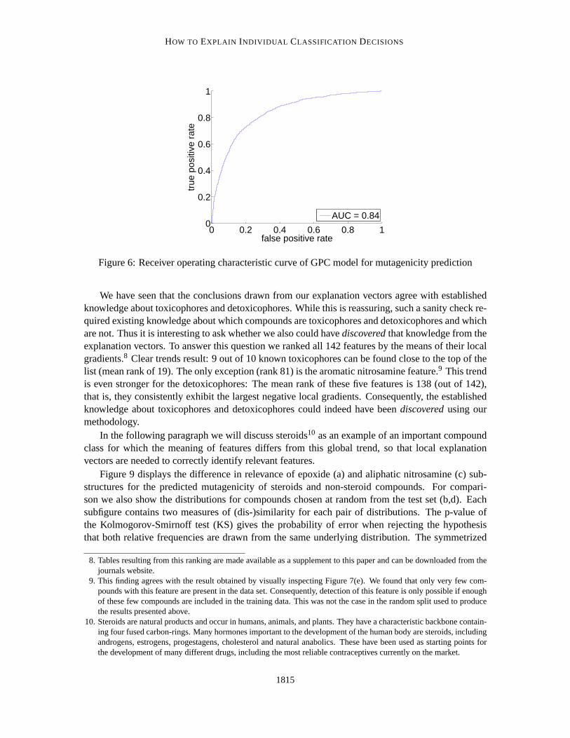
• Performance (84 % area under curve) confirms our previous results (Hansen et al., 2009).Error rates can be obtained from Figure 6.

Together with the prediction we calculated the explanation vector (as introduced in Definition 2) foreach test point. The remainder of this Section is an evaluation of these local explanations.

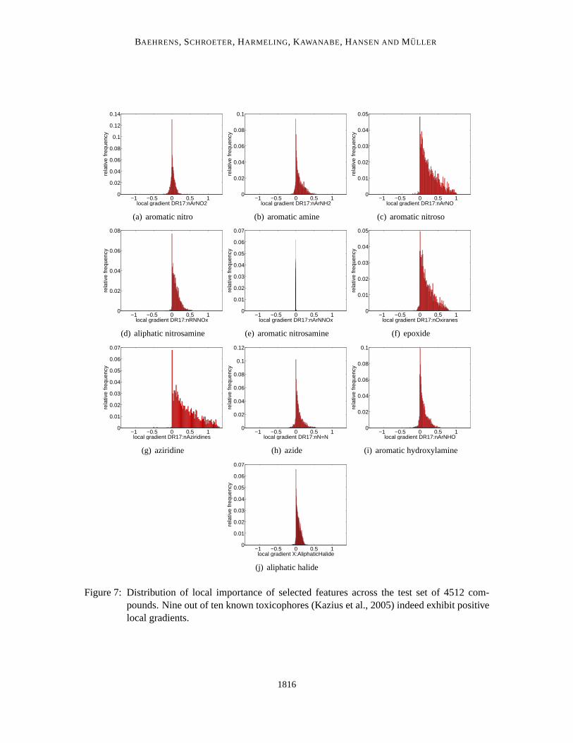
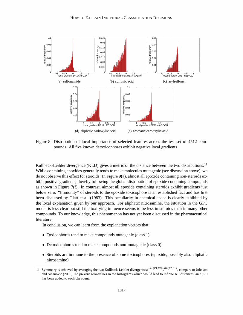
In Figures 7 and 8 we show the distribution of the local importance of selectedfeatures acrossthe test set: For each input feature we generate a histogram of local importance values, as indicatedby its corresponding entry in the explanation vector of each of the 4512 test compounds. Thefeatures examined in Figure 7 are counts of substructures known to cause mutagenicity. We showall approved “specific toxicophores” introduced by Kazius et al. (2005) that are also representedin the DRAGON set of features. The features shown in Figure 8 are known to detoxify certaintoxicophores (again see Kazius et al., 2005). With the exception of 7(e) the toxicophores also havea toxifying influence according to our GPC prediction model. Feature 7(e) seems to be mostlyirrelevant for the prediction of the GPC model on the test points. In contrast the detoxicophoresshow overall negative influence on the prediction outcome of the GPC model.Modifying the testcompounds by adding toxicophores will increase the probability of being mutagenic as predicted bythe GPC model while adding detoxicophores will decrease this predicted probability.

7. See Hansen et al. (2009) for results of modeling this set using different machine learning methods. The data itself isavailable online athttp://ml.cs.tu-berlin.de/toxbenchmark .

1814


0 0.2 0.4 0.6 0.8 10

0.2

0.4

0.6

0.8

1

false positive rate

true

pos

itive

rat

e

AUC = 0.84

Figure 6: Receiver operating characteristic curve of GPC model for mutagenicity prediction

We have seen that the conclusions drawn from our explanation vectors agree with establishedknowledge about toxicophores and detoxicophores. While this is reassuring, such a sanity check re-quired existing knowledge about which compounds are toxicophores anddetoxicophores and whichare not. Thus it is interesting to ask whether we also could havediscoveredthat knowledge from theexplanation vectors. To answer this question we ranked all 142 featuresby the means of their localgradients.8 Clear trends result: 9 out of 10 known toxicophores can be found closeto the top of thelist (mean rank of 19). The only exception (rank 81) is the aromatic nitrosamine feature.9 This trendis even stronger for the detoxicophores: The mean rank of these five features is 138 (out of 142),that is, they consistently exhibit the largest negative local gradients. Consequently, the establishedknowledge about toxicophores and detoxicophores could indeed havebeendiscoveredusing ourmethodology.

In the following paragraph we will discuss steroids10 as an example of an important compoundclass for which the meaning of features differs from this global trend, sothat local explanationvectors are needed to correctly identify relevant features.

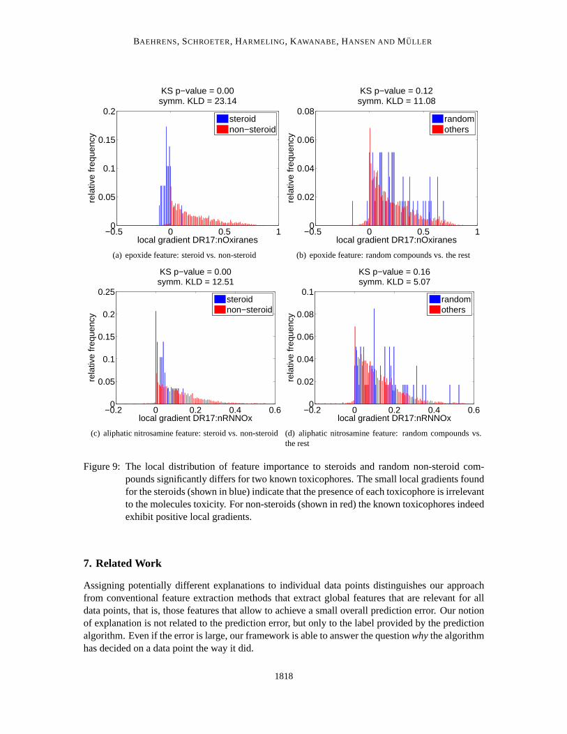
Figure 9 displays the difference in relevance of epoxide (a) and aliphatic nitrosamine (c) sub-structures for the predicted mutagenicity of steroids and non-steroid compounds. For compari-son we also show the distributions for compounds chosen at random fromthe test set (b,d). Eachsubfigure contains two measures of (dis-)similarity for each pair of distributions. The p-value ofthe Kolmogorov-Smirnoff test (KS) gives the probability of error when rejecting the hypothesisthat both relative frequencies are drawn from the same underlying distribution. The symmetrized

8. Tables resulting from this ranking are made available as a supplement tothis paper and can be downloaded from thejournals website.

9. This finding agrees with the result obtained by visually inspecting Figure 7(e). We found that only very few com-pounds with this feature are present in the data set. Consequently, detection of this feature is only possible if enoughof these few compounds are included in the training data. This was not the case in the random split used to producethe results presented above.

10. Steroids are natural products and occur in humans, animals, and plants. They have a characteristic backbone contain-ing four fused carbon-rings. Many hormones important to the development of the human body are steroids, includingandrogens, estrogens, progestagens, cholesterol and natural anabolics. These have been used as starting points forthe development of many different drugs, including the most reliable contraceptives currently on the market.

1815


−1 −0.5 0 0.5 10

0.02

0.04

0.06

0.08

0.1

0.12

0.14

local gradient DR17:nArNO2

rela

tive

freq

uenc

y

(a) aromatic nitro

−1 −0.5 0 0.5 10

0.02

0.04

0.06

0.08

0.1

local gradient DR17:nArNH2

rela

tive

freq

uenc

y

(b) aromatic amine

−1 −0.5 0 0.5 10

0.01

0.02

0.03

0.04

0.05

local gradient DR17:nArNO

rela

tive

freq

uenc

y

(c) aromatic nitroso

−1 −0.5 0 0.5 10

0.02

0.04

0.06

0.08

local gradient DR17:nRNNOx

rela

tive

freq

uenc

y

(d) aliphatic nitrosamine

−1 −0.5 0 0.5 10

0.01

0.02

0.03

0.04

0.05

0.06

0.07

local gradient DR17:nArNNOx

rela

tive

freq

uenc

y

(e) aromatic nitrosamine

−1 −0.5 0 0.5 10

0.01

0.02

0.03

0.04

0.05

local gradient DR17:nOxiranes

rela

tive

freq

uenc

y

(f) epoxide

−1 −0.5 0 0.5 10

0.01

0.02

0.03

0.04

0.05

0.06

0.07

local gradient DR17:nAziridines

rela

tive

freq

uenc

y

(g) aziridine

−1 −0.5 0 0.5 10

0.02

0.04

0.06

0.08

0.1

0.12

local gradient DR17:nN=N

rela

tive

freq

uenc

y

(h) azide

−1 −0.5 0 0.5 10

0.02

0.04

0.06

0.08

0.1

local gradient DR17:nArNHO

rela

tive

freq

uenc

y

(i) aromatic hydroxylamine

−1 −0.5 0 0.5 10

0.01

0.02

0.03

0.04

0.05

0.06

0.07

local gradient X:AliphaticHalide

rela

tive

freq

uenc

y

(j) aliphatic halide

Figure 7: Distribution of local importance of selected features across the test set of 4512 com-pounds. Nine out of ten known toxicophores (Kazius et al., 2005) indeed exhibit positivelocal gradients.

1816


−1 −0.5 0 0.5 10

0.02

0.04

0.06

0.08

0.1

local gradient DR17:nSO2N

rela

tive

freq

uenc

y

(a) sulfonamide

−1 −0.5 0 0.5 10

0.005

0.01

0.015

0.02

0.025

0.03

0.035

local gradient DR17:nSO2OH

rela

tive

freq

uenc

y

(b) sulfonic acid

−1 −0.5 0 0.5 10

0.01

0.02

0.03

0.04

0.05

local gradient DR17:nS(=O)2

rela

tive

freq

uenc

y

(c) arylsulfonyl

−1 −0.5 0 0.5 10

0.01

0.02

0.03

0.04

0.05

local gradient DR17:nRCOOH

rela

tive

freq

uenc

y

(d) aliphatic carboxylic acid

−1 −0.5 0 0.5 10

0.02

0.04

0.06

0.08

0.1

local gradient DR17:nArCOOHre

lativ

e fr

eque

ncy

(e) aromatic carboxylic acid

Figure 8: Distribution of local importance of selected features across the test set of 4512 com-pounds. All five known detoxicophores exhibit negative local gradients

Kullback-Leibler divergence (KLD) gives a metric of the distance between the two distributions.11

While containing epoxides generally tends to make molecules mutagenic (see discussion above), wedo not observe this effect for steroids: In Figure 9(a), almost all epoxide containing non-steroids ex-hibit positive gradients, thereby following the global distribution of epoxidecontaining compoundsas shown in Figure 7(f). In contrast, almost all epoxide containing steroids exhibit gradients justbelow zero. “Immunity” of steroids to the epoxide toxicophore is an established fact and has firstbeen discussed by Glatt et al. (1983). This peculiarity in chemical space isclearly exhibited bythe local explanation given by our approach. For aliphatic nitrosamine, thesituation in the GPCmodel is less clear but still the toxifying influence seems to be less in steroids than in many othercompounds. To our knowledge, this phenomenon has not yet been discussed in the pharmaceuticalliterature.

In conclusion, we can learn from the explanation vectors that:

• Toxicophores tend to make compounds mutagenic (class 1).

• Detoxicophores tend to make compounds non-mutagenic (class 0).

• Steroids are immune to the presence of some toxicophores (epoxide, possibly also aliphaticnitrosamine).

11. Symmetry is achieved by averaging the two Kullback-Leibler divergences:KL(P1,P2)+KL(P2,P1)2 , compare to Johnson

and Sinanovic (2000). To prevent zero-values in the histograms whichwould lead to infinite KL distances, anε > 0has been added to each bin count.

1817


−0.5 0 0.5 10

0.05

0.1

0.15

0.2

KS p−value = 0.00symm. KLD = 23.14


rela

tive

freq

uenc

y

steroidnon−steroid

(a) epoxide feature: steroid vs. non-steroid

−0.5 0 0.5 10

0.02

0.04

0.06

0.08



rela

tive

freq

uenc

y

randomothers

(b) epoxide feature: random compounds vs. the rest

−0.2 0 0.2 0.4 0.60

0.05

0.1

0.15

0.2

0.25



rela

tive

freq

uenc

y

steroidnon−steroid

(c) aliphatic nitrosamine feature: steroid vs. non-steroid

−0.2 0 0.2 0.4 0.60

0.02

0.04

0.06

0.08

0.1



rela

tive

freq

uenc

y

randomothers

(d) aliphatic nitrosamine feature: random compounds vs.the rest

Figure 9: The local distribution of feature importance to steroids and random non-steroid com-pounds significantly differs for two known toxicophores. The small localgradients foundfor the steroids (shown in blue) indicate that the presence of each toxicophore is irrelevantto the molecules toxicity. For non-steroids (shown in red) the known toxicophores indeedexhibit positive local gradients.

7. Related Work

Assigning potentially different explanations to individual data points distinguishes our approachfrom conventional feature extraction methods that extract global features that are relevant for alldata points, that is, those features that allow to achieve a small overall prediction error. Our notionof explanation is not related to the prediction error, but only to the label provided by the predictionalgorithm. Even if the error is large, our framework is able to answer the questionwhythe algorithmhas decided on a data point the way it did.

1818


The explanation vector proposed here is similar in spirit to sensitivity analysiswhich is commonin various areas of information science. A classical example is outlier sensitivity in statistics (Ham-pel et al., 1986). In this case, the effects of removing single data points onestimated parametersare evaluated by an influence function. If the influence for a data point issignificantly large, it isdetected as an outlier and should be removed for the following analysis. In regression problems,leverage analysis is a procedure along similar lines. It detects leverage points which have potentialto give large impact on the estimate of the regression function. In contrast tothe influential points(outliers), removing a leverage sample may not actually change the regressor, if its response is veryclose to the predicted value. E.g., for linear regression the samples whose inputs are far from themean are the leverage points. Our framework of explanation vectors considers a different view. Itdescribes the influence ofmovingsingle data points locally and it thus answers the question whichdirections are locally most influential to the prediction. The explanation vectors are used to extractsensitive features that are relevant to the prediction results, rather thandetecting/eliminating theinfluential samples.

In recent decades, explanation of results by expert systems has beenan important topic in theArtificial Intelligence community. Especially for expert systems based on Bayesian belief networks,such explanation is crucial in practical use. In this context sensitivity analysis has also been usedas a guiding principle (Horvitz et al., 1988). There the influence is evaluated by removing a set ofvariables (features) from the evidence and the explanation is constructed from those variables thataffect inference (relevant variables). For example, Suermondt (1992) measures the cost of omittinga single featureEi by the cross-entropy

H−(Ei) = H(p(D|E);P(D|E\Ei)) =N

∑j=1

P(d j |E) logP(d j |E)

p(d j |E\Ei),

whereE denotes the evidence andD = (d1, . . . ,dN)T is the target variable. The cost of a subset

F ⊂ E can be defined similarly. This line of research is more connected to our work, becauseexplanation can depend on the assigned values of the evidenceE, and is thus local.

Similarly Robnik-Sikonja and Kononenko (2008) and Strumbelj and Kononenko (2008) try toexplain the decision of trained kNN-, SVM-, and ANN-models for individual instances by measur-ing the difference in their prediction with sets of features omitted. The cost ofomitting featuresis evaluated as the information difference, the log-odds ratio, or the difference of probabilities be-tween the model with knowledge about all features and with omissions, respectively. To know whatthe prediction would be without the knowledge of a certain feature the model is retrained for everychoice of features whose influence is to be explained. To save the time of combinatorial trainingRobnik-Sikonja and Kononenko (2008) propose to use neutral valueswhich have to be estimatedby a known prior distribution of all possible parameter values. As a theoretical framework for con-sidering feature interactions, Strumbelj and Kononenko (2008) propose to calculate the differencesbetween model predictions for every choice of feature subset.

For multi-layer perceptrons Fraud and Clrot (2002) measure the importance of individual in-put variables on clusters of test points. Therefore the change in the modeloutput is evaluated forthe change of a single input variable in a chosen interval while all other input variables are fixed.Lemaire and Feraud (2007) use a similar approach on an instance by instance basis. By consideringeach input variable in turn there is no way to measure input feature interactions on the model output(see LeCun et al., 1998).

1819


p( | )y=1 x

x1

x1

x2

0.5

Figure 10:ζ(x) is the zero vector in the middle of the cluster in the middle.

The principal differences between our approach and these frameworks are: (i) We considercontinuous features and no structure among them is required, while some other frameworks startfrom binary features and may require discretization steps with the need to estimate parameters forit. (ii) We allow changes in any direction, that is, any weighted combination of variables, whileother approaches only consider one feature at a time or the omission of a set of variables.

8. Discussion

We have shown that our methods for calculating / estimating explanation vectors are useful in avariety of situations. In the following we discuss their limitations.

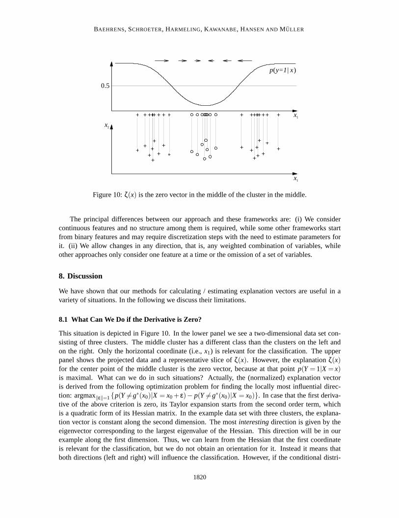
8.1 What Can We Do if the Derivative is Zero?

This situation is depicted in Figure 10. In the lower panel we see a two-dimensional data set con-sisting of three clusters. The middle cluster has a different class than the clusters on the left andon the right. Only the horizontal coordinate (i.e.,x1) is relevant for the classification. The upperpanel shows the projected data and a representative slice ofζ(x). However, the explanationζ(x)for the center point of the middle cluster is the zero vector, because at thatpoint p(Y=1|X= x)is maximal. What can we do in such situations? Actually, the (normalized) explanation vectoris derived from the following optimization problem for finding the locally most influential direc-tion: argmax‖ε‖=1{p(Y 6=g∗(x0)|X = x0+ ε)− p(Y 6=g∗(x0)|X = x0)}. In case that the first deriva-tive of the above criterion is zero, its Taylor expansion starts from the second order term, whichis a quadratic form of its Hessian matrix. In the example data set with three clusters, the explana-tion vector is constant along the second dimension. The mostinterestingdirection is given by theeigenvector corresponding to the largest eigenvalue of the Hessian. This direction will be in ourexample along the first dimension. Thus, we can learn from the Hessian thatthe first coordinateis relevant for the classification, but we do not obtain an orientation for it. Instead it means thatboth directions (left and right) will influence the classification. However, ifthe conditional distri-

1820


butionP(Y = 1 | X = x) is flat in some regions, no meaningful explanation can be obtained by thegradient-based approach with the remedy mentioned above. Practically, byusing Parzen windowestimators with larger widths, the explanation vector can capture coarse structures of the classifierat the points that are not so far from the borders. In A.3.2 we give an illustration of this point. In thefuture, we would like to work on global approaches, for example, basedon distances to the borders,or extensions of the approach by Robnik-Sikonja and Kononenko (2008). Since these proceduresare expected to be computationally demanding, our proposal is useful in practice, in particular forprobabilistic classifiers.

8.2 Does Our Framework Generate Different Explanations for Different Prediction Models?

When using the local gradient of the model prediction directly as in Definition 2and Section 6,the explanation follows the given model precisely by definition. For the estimation framework thisdepends on whether the different classifiers classify the data differently. In that case the explanationvectors will be different, which makes sense, since they should explain theclassifier at hand, evenif its estimated labels were not all correct. On the other hand, if the differentclassifiers agree on alllabels, the explanation will be exactly equal.

8.3 Which Implicit Limitations Do Analytical Gradients Inherit From Gaussia n ProcessModels?

A particular phenomenon can be observed at the boundaries of the training data: Far from thetraining data, Gaussian Process Classification models predict a probability of 0.5 for the positiveclass. When querying the model in an area of the feature space where predictions are negative,and one approaches the boundaries of the space populated with training data, explanation vectorswill point away from any training data and therefore also away from areas of positive prediction.This behavior can be observed in Figure 1(d), where unit length vectors indicate the direction ofexplanation vectors. In the right hand side corner, arrows point awayfrom the triangle. However,we can see that the length of these vectors is so small that they are not evenvisible in Figure1(c). Consequently, this property of GPC models does not pose a restriction for identifying thelocally most influential features by investigating the features with the highest absolute values in therespective partial derivatives, as shown in Section 6.

8.4 Stationarity of the Data

Since explanation vectors are defined as local gradients of the model prediction (see Definition 2),no assumption on the data is made: The local gradients follow the predictive model in any case. If,however, the model to be explained assumes stationarity of the data, the explanation vectors willinherit this limitation and reflect any shortcomings of the model (e.g., when the model is appliedto non-stationary data). Our method for estimating explanation vectors, on theother hand, assumesstationarity of the data.

When modeling data that is in fact non-stationary, appropriate measures to deal with such datasets should be taken. One option is to separate the feature space into stationary and non-stationaryparts using Stationary Subspace Analysis as introduced by von Bunau et al. (2009). For furtherapproaches to data set shift see Sugiyama et al. (2007b), Sugiyama et al. (2007a), and the book byQuionero-Candela et al. (2009).

1821


9. Conclusion

This paper proposes a method that sheds light on the black boxes of nonlinear classifiers. In otherwords, we introduce a method that can explain the local decisions taken by arbitrary (possibly)nonlinear classification algorithms. In a nutshell, the estimated explanations arelocal gradients thatcharacterize how a data point has to be moved to change its predicted label. For models where suchgradient information cannot be calculated explicitly, we employ a probabilistic approximate mimicof the learning machine to be explained.

To validate our methodology we show how it can be used to draw new conclusions on how thevarious Iris flowers in Fisher’s famous data set are different from each other and how to identifythe features with which certain types of digits 2 and 8 in the USPS data set can be distinguished.Furthermore, we applied our method to a challenging drug discovery problem. The results on thatdata fully agree with existing domain knowledge, which was not available to ourmethod. Evenlocal peculiarities in chemical space (the extraordinary behavior of steroids) was discovered usingthe local explanations given by our approach.

Future directions are two-fold: First we believe that our method will find its way into the toolboxes of practitioners who not only want to automatically classify their data but who also wouldlike to understand the learned classifier. Thus using our explanation framework in computationalbiology (see Sonnenburg et al., 2008) and in decision making experiments inpsychophysics (e.g.,Kienzle et al., 2009) seems most promising. The second direction is to generalize our approach toother prediction problems such as regression.

Acknowledgments

This work was supported in part by the FP7-ICT Programme of the European Community, underthe PASCAL2 Network of Excellence, ICT-216886 and by DFG Grant MU987/4-1. We would liketo thank Andreas Sutter, Antonius Ter Laak, Thomas Steger-Hartmann andNikolaus Heinrich forpublishing the Ames mutagenicity data set (Hansen et al., 2009).

Appendix A.

In the following we present the derivation of direct local gradients and illustrate aspects like theeffect of different kernel functions, outliers and local non-linearities. Furthermore we present thederivation of explanation vectors based on the parzen window estimation and illustrate how thequality of the fit of the Parzen window approximation affects the quality of the estimated explanationvectors.

A.1 Derivation of Direct Local Gradients

Equation (1) is derived by the following steps:

1822


∇p(x)|x=x0

=∇12

erfc

(

− f (x)√2∗√

1+varf (x)

)∣

∣

∣

∣

∣

x=x0

=∇12

(

1−erf

(

− f (x)√2∗√

1+varf (x)

))∣

∣

∣

∣

∣

x=x0

=− 12

∇ erf

(

− f (x)√2∗√

1+varf (x)

)∣

∣

∣

∣

∣

x=x0

=−exp(

− f (x0)2

2(1+varf (x0))

)

√π

∇

(

− f (x)√2∗√

1+varf (x)

)∣

∣

∣

∣

∣

x=x0

=−exp(

− f (x0)2

2(1+varf (x0))

)

√π

(

− 1√2

∇

(

f (x)√

1+varf (x)

)∣

∣

∣

∣

∣

x=x0

)

=exp(

− f (x0)2

2(1+varf (x0))

)

√2π

(

∇ f (x)|x=x0√

1+varf (x0)+ f (x0)

(

∇ varf (x)∣

∣

x=x0∗−1

2(1+varf (x0))

− 32

))

=exp(

− f (x0)2

2(1+varf (x0))

)

√2π

(

∇ f (x)|x=x0√

1+varf (x0)− 1

2f (x0)

(1+varf (x0))32

∇varf (x)|x=x0

)

.

A.2 Illustration of Direct Local Gradients

In the following we give some illustrative examples of our method to explain modelsusing localgradients. Since the explanation is derived directly from the respective model, it is interesting toinvestigate its acurateness depending on different model parameters andin instructive scenarios.We examine the effects that local gradients exhibit when choosing different kernel functions, whenintroducing outliers, and when the classes are not linearly separable locally.

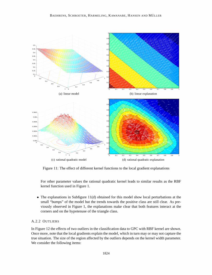
A.2.1 CHOICE OFKERNEL FUNCTION

Figure 11 shows the effect of different kernel functions on the triangle toy data from Figure 1. Thefollowing observations can be made:

• In any case note that the local gradients explain the model, which in turn may ormay notcapture the true situation.

• In Subfigure 11(a) the linear kernel leads to a model which fails to capturethe non-linear classseparation. This model misspecification is reflected by the explanations given for this modelin Subfigure 11(b).

• The rational quadratic kernel is able to more accurately model the non-linear separation. InSubfigure 11(c) a non-optimal degree parameter has been chosen forillustrative purposes.

1823


0

0.2

0.4

0.6

0.8

1 00.2

0.40.6

0.81

0.1

0.15

0.2

0.25

0.3

0.35

0.4

0.45

0.5

(a) linear model

0 0.1 0.2 0.3 0.4 0.5 0.6 0.7 0.8 0.9 10

0.1

0.2

0.3

0.4

0.5

0.6

0.7

0.8

0.9

1

(b) linear explanation

0

0.2

0.4

0.6

0.8

1 00.2

0.40.6

0.81

0.303

0.3032

0.3034

0.3036

0.3038

0.304

0.3042

(c) rational quadratic model

0 0.1 0.2 0.3 0.4 0.5 0.6 0.7 0.8 0.9 10

0.1

0.2

0.3

0.4

0.5

0.6

0.7

0.8

0.9

1

(d) rational quadratic explanation

Figure 11: The effect of different kernel functions to the local gradient explanations

For other parameter values the rational quadratic kernel leads to similar results as the RBFkernel function used in Figure 1.

• The explanations in Subfigure 11(d) obtained for this model show local perturbations at thesmall “bumps” of the model but the trends towards the positive class are still clear. As pre-viously observed in Figure 1, the explanations make clear that both features interact at thecorners and on the hypotenuse of the triangle class.

A.2.2 OUTLIERS

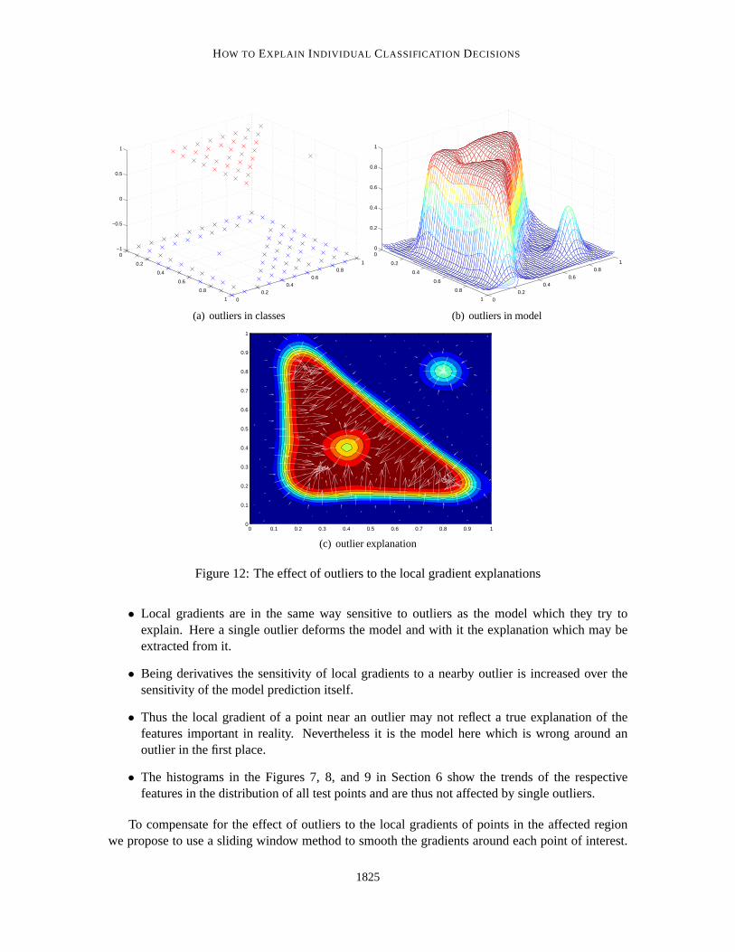
In Figure 12 the effects of two outliers in the classification data to GPC with RBF kernel are shown.Once more, note that the local gradients explain the model, which in turn may or may not capture thetrue situation. The size of the region affected by the outliers depends on thekernel width parameter.We consider the following items:

1824


0

0.2

0.4

0.6

0.8

1 00.2

0.40.6

0.81

−1

−0.5

0

0.5

1

(a) outliers in classes

0

0.2

0.4

0.6

0.8

1 00.2

0.40.6

0.81

0

0.2

0.4

0.6

0.8

1

(b) outliers in model

0 0.1 0.2 0.3 0.4 0.5 0.6 0.7 0.8 0.9 10

0.1

0.2

0.3

0.4

0.5

0.6

0.7

0.8

0.9

1

(c) outlier explanation

Figure 12: The effect of outliers to the local gradient explanations

• Local gradients are in the same way sensitive to outliers as the model which they try toexplain. Here a single outlier deforms the model and with it the explanation whichmay beextracted from it.

• Being derivatives the sensitivity of local gradients to a nearby outlier is increased over thesensitivity of the model prediction itself.

• Thus the local gradient of a point near an outlier may not reflect a true explanation of thefeatures important in reality. Nevertheless it is the model here which is wrongaround anoutlier in the first place.

• The histograms in the Figures 7, 8, and 9 in Section 6 show the trends of the respectivefeatures in the distribution of all test points and are thus not affected by single outliers.

To compensate for the effect of outliers to the local gradients of points in theaffected regionwe propose to use a sliding window method to smooth the gradients around eachpoint of interest.

1825


Thus for each point use the mean of all local gradients in the hypercube centered at this point andof appropriate size. This way the disrupting effect of an outlier is averaged out for an appropriatelychosen window size.

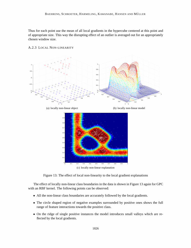
A.2.3 LOCAL NON-LINEARITY

0

0.2

0.4

0.6

0.8

1 00.2

0.40.6

0.81

−1

−0.5

0

0.5

1

(a) locally non-linear object

0

0.2

0.4

0.6

0.8

1 00.2

0.40.6

0.81

0

0.2

0.4

0.6

0.8

1

(b) locally non-linear model

0 0.1 0.2 0.3 0.4 0.5 0.6 0.7 0.8 0.9 10

0.1

0.2

0.3

0.4

0.5

0.6

0.7

0.8

0.9

1

(c) locally non-linear explanation

Figure 13: The effect of local non-linearity to the local gradient explanations

The effect of locally non-linear class boundaries in the data is shown in Figure 13 again for GPCwith an RBF kernel. The following points can be observed:

• All the non-linear class boundaries are accurately followed by the local gradients.

• The circle shaped region of negative examples surrounded by positiveones shows the fullrange of feature interactions towards the positive class.

• On the ridge of single positive instances the model introduces small valleys which are re-flected by the local gradients.

1826


A.3 Estimating by Parzen Window

Finally we elaborate on some details of our estimation approach of local gradients by Parzen windowapproximation. First we give the derivation to obtain the explanation vector and second we examinehow the explanation varies with the goodness of fit of the Parzen window method.

A.3.1 DERIVATION OF EXPLANATION VECTORS

These are more details on the derivation of Definition 3. We use the index setIc = {i | g(xi) = c}:

∂∂x

kσ(x) =− xσ2kσ(x)

∂∂x

pσ(x,y 6=c) =1n ∑

i /∈Ic

kσ(x−xi)−(x−xi)

σ2

∂∂x

pσ(y 6=c|x)

=

(

∑i /∈Ic k(x−xi))(

∑ni=1k(x−xi)(x−xi)

)

σ2(

∑ni=1k(z−xi)

)2

−

(

∑i /∈Ic k(x−xi)(x−xi))(

∑ni=1k(x−xi)

)

σ2(

∑ni=1k(z−xi)

)2

=

(

∑i /∈Ic k(x−xi))(

∑i∈Ic k(x−xi)(x−xi))

σ2(

∑ni=1k(z−xi)

)2

−

(

∑i /∈Ic k(x−xi)(x−xi))(

∑i∈Ic k(x−xi))

σ2(

∑ni=1k(z−xi)

)2

and thus for the index setIg(z) = {i | g(xi) = g(z)}

ζ(z) =∂∂x

p(y 6=g(z) | x)

∣

∣

∣

∣

x=z

=

(

∑i /∈Ig(z) k(z−xi))(

∑i∈Ig(z) k(z−xi)(z−xi))

σ2(

∑ni=1k(z−xi)

)2

−

(

∑i /∈Ig(z) k(z−xi)(z−xi))(

∑i∈Ig(z) k(z−xi))

σ2(

∑ni=1k(z−xi)

)2 .

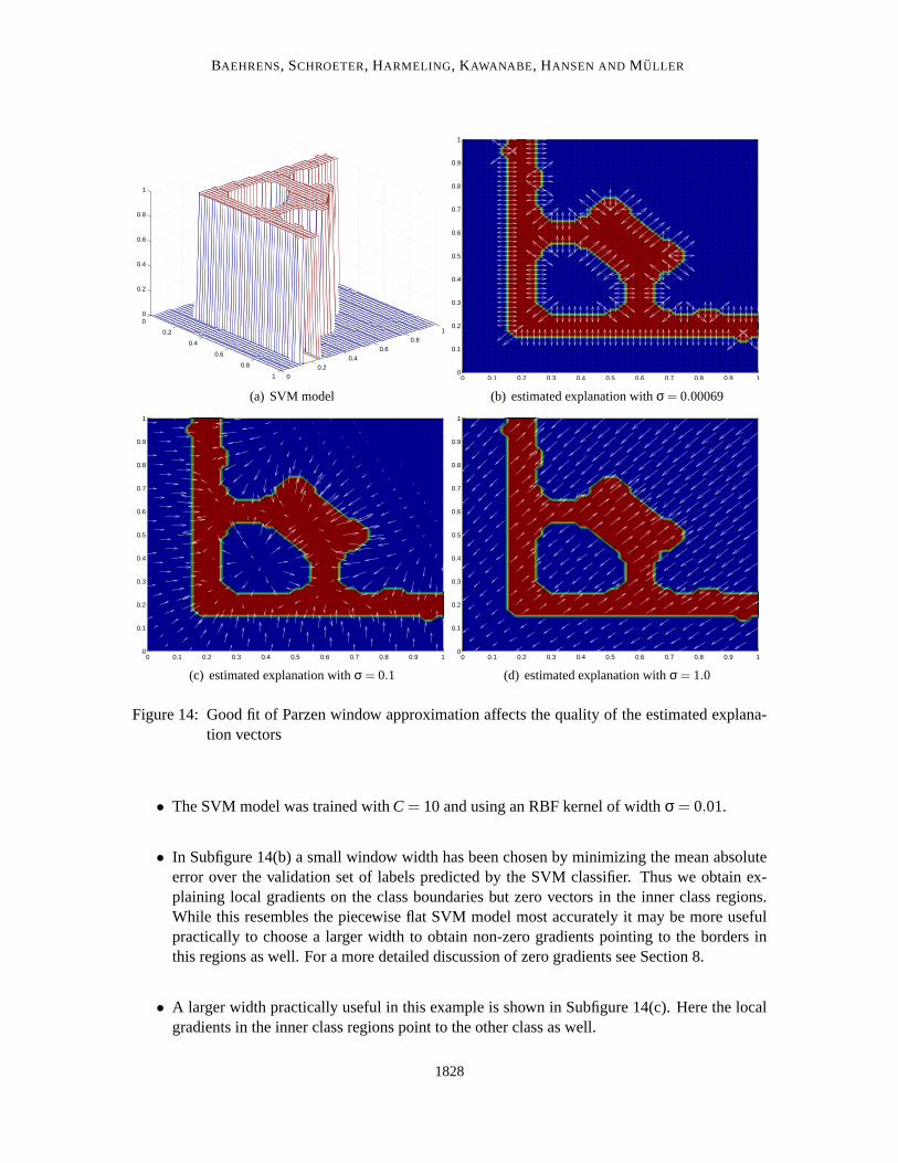
A.3.2 GOODNESS OFFIT BY PARZEN WINDOW

In our estimation framework the quality of the local gradients depends on the approximation of theclassifier we want to explain by Parzen windows for which we can calculatethe explanation vectorsas given by Definition 3.

Figure 14(a) shows an SVM model trained on the classification data from Figure 13(a). Thelocal gradients estimated for this model by different Parzen window approximations are depicted inSubfigures 14(b), 14(c), and 14(d). We observe the following points:

1827


0

0.2

0.4

0.6

0.8

1 00.2

0.40.6

0.81

0

0.2

0.4

0.6

0.8

1

(a) SVM model

0 0.1 0.2 0.3 0.4 0.5 0.6 0.7 0.8 0.9 10

0.1

0.2

0.3

0.4

0.5

0.6

0.7

0.8

0.9

1

(b) estimated explanation withσ = 0.00069

0 0.1 0.2 0.3 0.4 0.5 0.6 0.7 0.8 0.9 10

0.1

0.2

0.3

0.4

0.5

0.6

0.7

0.8

0.9

1

(c) estimated explanation withσ = 0.1

0 0.1 0.2 0.3 0.4 0.5 0.6 0.7 0.8 0.9 10

0.1

0.2

0.3

0.4

0.5

0.6

0.7

0.8

0.9

1

(d) estimated explanation withσ = 1.0

Figure 14: Good fit of Parzen window approximation affects the quality of the estimated explana-tion vectors

• The SVM model was trained withC= 10 and using an RBF kernel of widthσ = 0.01.

• In Subfigure 14(b) a small window width has been chosen by minimizing the meanabsoluteerror over the validation set of labels predicted by the SVM classifier. Thus we obtain ex-plaining local gradients on the class boundaries but zero vectors in the inner class regions.While this resembles the piecewise flat SVM model most accurately it may be more usefulpractically to choose a larger width to obtain non-zero gradients pointing to theborders inthis regions as well. For a more detailed discussion of zero gradients see Section 8.

• A larger width practically useful in this example is shown in Subfigure 14(c).Here the localgradients in the inner class regions point to the other class as well.

1828


• For a too large window width in Subfigure 14(d) the approximation fails to obtainlocal gra-dients which closely follow the model. Here only two directions are left and the gradients forthe blue class on the left and on the bottom point in the wrong direction.

References

B. N. Ames, E. G. Gurney, J. A. Miller, and H. Bartsch. Carcinogens asframeshift mutagens:Metabolites and derivatives of 2-acetylaminofluorene and other aromatic amine carcinogens.Pro-ceedings of the National Academy of Sciences of the United States of America, 69(11):3128–3132,1972.

C.M. Bishop.Neural Networks for Pattern Recognition. Oxford University Press, 1995.

L. Devroye, L. Gyorfi, and G. Lugosi.A Probabilistic Theory of Pattern Recognition. Number 31in Applications of Mathematics. Springer, New York, 1996.

R.A. Fisher. The use of multiple measurements in taxonomic problems.Annals of Eugenics, 7:179–188, 1936.

R. Fraud and F. Clrot. A methodology to explain neural network classification. Neural Networks,15(2):237 – 246, 2002. doi: 10.1016/S0893-6080(01)00127-7.

H. Glatt, R. Jung, and F. Oesch. Bacterial mutagenicity investigation of epoxides: drugs, drugmetabolites, steroids and pesticides.Mutation Research/Fundamental and Molecular Mecha-nisms of Mutagenesis, 111(2):99–118, 1983. doi: 10.1016/0027-5107(83)90056-8.

I. Guyon and A. Elisseeff. An introduction to variable and feature selection. The Journal of MachineLearning Research, 3:1157–1182, 2003.

F. R. Hampel, E. M. Ronchetti, P. J. Rousseeuw, and W. A. Stahel.Robust Statistics: The ApproachBased on Influence Functions. Wiley, New York, 1986.

K. Hansen, S. Mika, T. Schroeter, A. Sutter, A. Ter Laak, T. Steger-Hartmann, N. Heinrich, andK.-R. Muller. A benchmark data set for in silico prediction of ames mutagenicity.Journal ofChemical Information and Modelling, 49(9):2077–2081, 2009.

T. Hastie, R. Tibshirani, and J. Friedman.The Elements of Statistical Learning. Springer, 2001.

E. J. Horvitz, J. S. Breese, and M. Henrion. Decision theory in expertsystems and artificial in-teligence.Journal of Approximation Reasoning, 2:247–302, 1988. Special Issue on Uncertaintyin Artificial Intelligence.

D. H. Johnson and S. Sinanovic. Symmetrizing the Kullback-Leibler distance. Technical report,IEEE Transactions on Information Theory, 2000.

J. Kazius, R. McGuire, and R. Bursi. Derivation and validation of toxicophores for mutagenicityprediction.J. Med. Chem., 48:312–320, 2005.

W. Kienzle, M. O. Franz, B. Scholkopf, and F. A. Wichmann. Center-surround patterns emerge asoptimal predictors for human saccade targets.Journal of Vision, 9(5):1–15, 2009.

1829


M. Kuss and C. E. Ramussen. Assesing approximate inference for binary gaussian process classifi-cation.Journal of Machine Learning Research, 6:1679–1704, 2005.

Y. LeCun, L. Bottou, G.B. Orr, and K.-R. Muller. Efficient backprop. In G.B. Orr and K.-R. Muller,editors,Neural Networks: Tricks of the Trade, pages 9–53. Springer, 1998.

V. Lemaire and R. Feraud. Une methode d’interpretation de scores. InEGC, pages 191–192, 2007.

K.-R. Muller, S. Mika, G. Ratsch, K. Tsuda, and B. Scholkopf. An introduction to kernel-basedlearning algorithms.Neural Networks, IEEE Transactions on, 12(2):181–201, 2001.

Olga Obrezanova and Matthew D. Segall. Gaussian processes for classification: QSAR modeling ofADMET and target activity.Journal of Chemical Information and Modeling, April 2010. ISSN1549-9596. doi: doi:10.1021/ci900406x. URLhttp://dx.doi.org/10.1021/ci900406x .

O. Obrezanova, G. Csanyi, J. M. R. Gola, and M. D. Segall. Gaussian processes: A method forautomatic QSAR modelling of adme properties.J. Chem. Inf. Model.

O. Obrezanova, J. M. R. Gola, E. J. Champness, and M. D. Segall. Automatic QSAR modeling ofadme properties: blood-brain barrier penetration and aqueous solubility.J. Comput.-Aided Mol.Des., 22:431–440, 2008.

J. C. Platt. Probabilistic outputs for support vector machines and comparisons to regularized likeli-hood methods. InAdvances in Large Margin Classifiers, pages 61–74. MIT Press, 1999.

J. Quionero-Candela, M. Sugiyama, A. Schwaighofer, and N. D. Lawrence. Dataset Shift in Ma-chine Learning. The MIT Press, 2009.

C. E. Rasmussen and C. K. I. Williams.Gaussian Processes for Machine Learning. Springer, 2006.

M. Robnik-Sikonja and I. Kononenko. Explaining classifications for individual instances.IEEETKDE, 20(5):589–600, 2008.

B. Scholkopf and A. Smola.Learning with Kernels. MIT, 2002.

T. Schroeter, A. Schwaighofer, S. Mika, A. Ter Laak, D. Suelzle, U.Ganzer, N. Heinrich, and K.-R.Muller. Estimating the domain of applicability for machine learning QSAR models: A study onaqueous solubility of drug discovery molecules.Journal of Computer Aided Molecular Design,21(9):485–498, 2007a.

T. Schroeter, A. Schwaighofer, S. Mika, A. Ter Laak, D. Suelzle, U.Ganzer, N. Heinrich, and K.-R.Muller. Machine learning models for lipophilicity and their domain of applicability.Mol. Pharm.,4(4):524–538, 2007b.

T. Schroeter, A. Schwaighofer, S. Mika, A. Ter Laak, D. Sulzle, U. Ganzer, N. Heinrich, and K.-R. Muller. Predicting lipophilicity of drug discovery molecules using gaussian process models.ChemMedChem, 2(9):1265–1267, 2007c.

A. Schwaighofer. SVM Toolbox for Matlab, Jan 2002. URLhttp://ida.first.fraunhofer.de/ ˜ anton/software.html .

1830


A. Schwaighofer, T. Schroeter, S. Mika, J. Laub, A. Ter Laak, D. Sulzle, U. Ganzer, N. Heinrich,and K.-R. Muller. Accurate solubility prediction with error bars for electrolytes: A machinelearning approach.Journal of Chemical Information and Modelling, 47(2):407–424, 2007.

A. Schwaighofer, T. Schroeter, S. Mika, K. Hansen, A. Ter Laak, P. Lienau, A. Reichel, N. Heinrich,and K.-R. Muller. A probabilistic approach to classifying metabolic stability.Journal of ChemicalInformation and Modelling, 48(4):785–796, 2008.

S. Sonnenburg, A. Zien, P. Philips, and G. Ratsch. POIMs: positional oligomer importance matrices— understanding support vector machine based signal detectors.Bioinformatics, 2008.

E. Strumbelj and I. Kononenko. Towards a model independent method for explaining classificationfor individual instances. In I.-Y. Song, J. Eder, and T.M. Nguyen, editors, Data Warehousingand Knowledge Discovery, volume 5182 ofLecture Notes in Computer Science, pages 273–282.Springer, 2008.

H. Suermondt.Explanation in Bayesian Belief Networks. PhD thesis, Department of ComputerScience and Medicine, Stanford University, Stanford, CA, 1992.

M. Sugiyama, M. Krauledat, and K.-R. Muller. Covariate shift adaptation by importance weightedcross validation.Journal of Machine Learning Research, 8:985–1005, May 2007a.

M. Sugiyama, S. Nakajima, H. Kashima, P. von Buenau, and M. Kawanabe.Direct importanceestimation with model selection and its application to covariate shift adaptation. InAdvances inNeural Information Processing Systems 20. MIT Press, 2007b.

R. Todeschini, V. Consonni, A. Mauri, and M. Pavan. DRAGON for Windows and Linux 2006.http://www.talete.mi.it/help/dragon_help/ (accessed 27 March 2009), 2006.

V. Vapnik. The Nature of Statistical Learning Theory. Springer, 1995.

P. von Bunau, F. C. Meinecke, F. J. Kiraly, and K.-R. Muller. Finding stationary subspaces inmultivariate time series.Physical Review Letters, 103(21):214101, 2009.

1831

How to Explain Individual Classiﬁcation...

Documents

Transcript of How to Explain Individual Classiﬁcation...