How to Excel - Part 1 - University of Cambridge · format to Excel (if you haven’t already done...

How to Excel - Part 1


Version: 1.0 24/10/2017 of 19

Table of Contents

Exercise 1a: Extract data from CUFS into Excel ............................................................... 4

Exercise 1b: Extract data from Cognos into Excel ........................................................... 5

General ledger report ........................................................................................................ 6

Grants report ..................................................................................................................... 7

Exercise 2: Basic formatting ..................................................................................................... 8

Task 1 – Unfreeze panes................................................................................................... 8

Task 2 – Delete columns ................................................................................................... 8

Task 3 – Resize columns................................................................................................... 8

Task 4 - Hide a column ...................................................................................................... 8

Task 5 – Freeze top row .................................................................................................... 9

Task 6 – Text wrapping ..................................................................................................... 9

Task 7 - Changing the presentation of minus numbers .................................................... 10

Task 8 – Subtotals ........................................................................................................... 10

Exercise 3: Basic formulas ............................................................................................... 11

Task 1 – AutoSum ........................................................................................................... 11

Task 2 – Multiplication ..................................................................................................... 11

Task 3 – Copying formulas .............................................................................................. 11

Task 4 – Division ............................................................................................................. 11

Task 5 – Recap ............................................................................................................... 11

Exercise 4: Quick guide to excel shortcuts..................................................................... 12

Exercise 5: Consolidation (1) ........................................................................................... 13

Task 1 ............................................................................................................................. 13

Task 2 ............................................................................................................................. 13

Task 3 ............................................................................................................................. 13

Task 4 ............................................................................................................................. 13

Task 5 ............................................................................................................................. 13

Task 6 ............................................................................................................................. 13

Task 7 ............................................................................................................................. 13


Version: 1.0 24/10/2017 of 19

Exercise 6: Advanced formulas ....................................................................................... 14

Task 1 - Formatting ......................................................................................................... 14

Task 2 – AVERAGE ........................................................................................................ 14

Task 3 – ABSOLUTE cell reference ................................................................................ 14

Task 4 – ROUND ............................................................................................................ 15

Task 5 – Adding .............................................................................................................. 15

Task 6 – IF function ......................................................................................................... 15

Task 7 – Test ................................................................................................................... 15

Exercise 7: Advanced formatting ..................................................................................... 16

Task 1 – Conditional formatting ....................................................................................... 16

Task 2 – Data validation .................................................................................................. 17

Task 3 – Sorting and subtotals (recap) ............................................................................ 17

Exercise 8: Consolidation (2) ........................................................................................... 18

Task 1 – Formatting and presentation ............................................................................. 18

Task 2 – Page headings .................................................................................................. 18

Task 3 – Data sorting ...................................................................................................... 18

Task 4 – IF function ......................................................................................................... 18

Task 5 – Conditional formatting ....................................................................................... 19

Task 6 – Data validation .................................................................................................. 19

Task 7 – Printing ............................................................................................................. 19


Version: 1.0 24/10/2017 of 19

Exercise 1a: Extract data from CUFS into Excel

Check that the report is not set to print by clicking on Options – the printer copies, if listed, should be set to zero

Click Submit

Once the report has run (click refresh data if it doesn’t show) select view output

When prompted select Save as and save the file to the desktop with the filename: Exercise1_CUFS_your initials

Once the file has downloaded, select Open and check that there is some data in the file before closing it down.

Log into CUFS with a GL responsibility

Select Reports > Standard >single request

In the name section select the list of values button

Select Account Analysis – Transaction Detail – Excel Version (UFS)


Version: 1.0 24/10/2017 of 19

Exercise 1b: Extract data from Cognos into Excel

From the main UFS page, select Admin/Cognos reporting and then Cognos Login

Select Log in to Cognos from the middle of the page and login with your Raven ID

Select Live

The correct school should be showing, open this folder

Select Departmental (Shared) Reports - this folder will contain GL Reporting and/or Grants Reporting folders

Select whichever one you would like to use


Version: 1.0 24/10/2017 of 19

General ledger report

Click the blue arrow to the right of the Financial Summary by Cost Centre – Long Report

Ensure that the delivery is set to View the report now and that the Prompt for values box is ticked

NB You can change the format to Excel at this point or once the report has run

Select Run

Complete any missing information and then select finish right at the bottom of the screen

Once the report has run you can change the format to Excel (if you haven’t already done so)

Select the format button at the top of the screen and then pick the appropriate Excel format

When prompted select Save as and save the file to the desktop with the filename:

Exercise1_CognosGL_your initials

Once the file has downloaded, select Open, check that there is some data and then close the file


Version: 1.0 24/10/2017 of 19

Grants report

Click the blue arrow to the right of the Detailed Expenditure Enquiry by Project

Ensure that the delivery is set to View the report now and that the Prompt for values box is ticked

NB You can change the format to Excel at this point or once the report has run

Select Run

Complete any missing information and then select finish right at the bottom of the screen

Once the report has run you can change the format to Excel (if you haven’t already done so)

Select the format button at the top of the screen and then pick the appropriate Excel format

When prompted select Save as and save the file to the desktop with the filename:

Exercise1_CognosGrants_your initials

Once the file has downloaded, select Open, check that there is some data and then close the file


Version: 1.0 24/10/2017 of 19

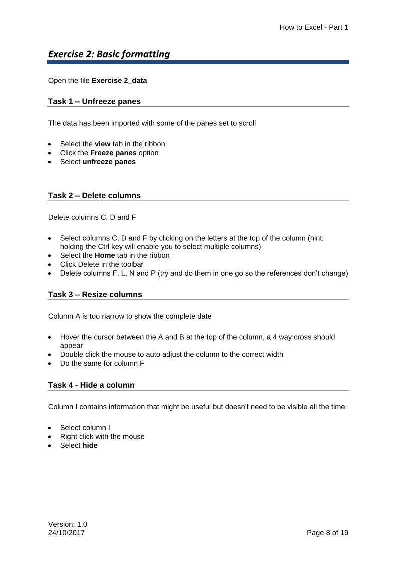
Exercise 2: Basic formatting

Open the file Exercise 2_data

Task 1 – Unfreeze panes

The data has been imported with some of the panes set to scroll

Select the view tab in the ribbon

Click the Freeze panes option

Select unfreeze panes

Task 2 – Delete columns

Delete columns C, D and F

Select columns C, D and F by clicking on the letters at the top of the column (hint: holding the Ctrl key will enable you to select multiple columns)

Select the Home tab in the ribbon

Click Delete in the toolbar

Delete columns F, L, N and P (try and do them in one go so the references don’t change)

Task 3 – Resize columns

Column A is too narrow to show the complete date

Hover the cursor between the A and B at the top of the column, a 4 way cross should appear

Double click the mouse to auto adjust the column to the correct width

Do the same for column F

Task 4 - Hide a column

Column I contains information that might be useful but doesn’t need to be visible all the time

Select column I

Right click with the mouse

Select hide


Version: 1.0 24/10/2017 of 19

Group function as an alternative to hiding columns and rows

Select the columns or rows that you want hidden

In the data tab select the group option

The section can be hidden and unhidden using the button at the top

Task 5 – Freeze top row

It can be easier to navigate a spreadsheet when the top row with the headings is fixed

Select the view tab in the ribbon

Click the Freeze panes option

Select freeze top row

Task 6 – Text wrapping

Sometimes the content of one cell is too wide for sensible width columns, the text wrapping function can be used to show the content on a wider row.

Select column H

Select the home tab in the ribbon

Click the Wrap text option

Manual resize the column by hovering between the two columns until the 4 way cross appears, click and drag to the desired width

Do the same with columns J and K


Version: 1.0 24/10/2017 of 19

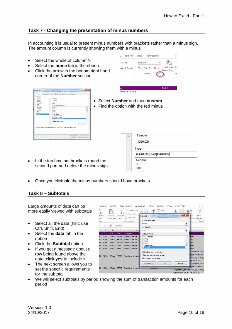
Task 7 - Changing the presentation of minus numbers

In accounting it is usual to present minus numbers with brackets rather than a minus sign. The amount column is currently showing them with a minus

Select the whole of column N

Select the home tab in the ribbon

Click the arrow in the bottom right hand corner of the Number section

Select Number and then custom

Find the option with the red minus

In the top box, put brackets round the second part and delete the minus sign

Once you click ok, the minus numbers should have brackets

Task 8 – Subtotals

Large amounts of data can be more easily viewed with subtotals

Select all the data (hint: use Ctrl, Shift, End)

Select the data tab in the ribbon

Click the Subtotal option

If you get a message about a row being found above the data, click yes to include it

The next screen allows you to set the specific requirements for the subtotal

We will select subtotals by period showing the sum of transaction amounts for each period


Version: 1.0 24/10/2017 of 19

Exercise 3: Basic formulas

Open the file Exercise 3_data

Task 1 – AutoSum

Scroll to the bottom of the data in column I

Select cell I80 and click AutoSum in the toolbar

It should select all of the data in the column

Click enter and the total should appear

Task 2 – Multiplication

In cell J1 enter the formula =I1*2

Task 3 – Copying formulas

In cell J1 hover the mouse over the bottom right hand corner until a black + appears

Double click with the mouse and the formula will be copied to every cell in the column

Task 4 – Division

In cell K1 enter the formula =J1/2

The answer should be the same as in column I Copy this formula to the whole column using the steps in task 3

Task 5 – Recap

Use the AutoSum function to total columns J and K

Be careful when you get to column K that the correct range is selected


Version: 1.0 24/10/2017 of 19

Exercise 4: Quick guide to excel shortcuts

Navigating a Spreadsheet

Ctrl + End Going to last cell containing data (the bottom right corner)

Ctrl + Shift + End Extends the selection of cells from the current point to the last used cell on the worksheet

Home Moves to the beginning of a row in a worksheet.

Ctrl + Home Returning to the top of your spreadsheet

Ctrl + Shift + Home Extends the selection of cells from the current point to the first used cell on the worksheet

Shift + arrow keys Selecting/highlighting a block of data

Ctrl + F / Shift + F5 Displays the Find window

Shift + F4 Repeats the last find action

Ctrl + H Find and replace window

Ctrl + A If the worksheet contains data, CTRL+A selects the current region. Pressing CTRL+A a second time selects the entire worksheet.

Shift + Arrow Key Extends the selection of cells by one cell.

Ctrl + Spacebar Selects an entire column in a worksheet.

Shift + Spacebar Selects an entire row in a worksheet.

Ctrl + Shift + Spacebar

Selects an entire worksheet. Repeat function if the worksheet contains data

Ctrl + Shift + Arrow Selects row or column of data

F5 or Ctrl + G Selects row or column of data


Version: 1.0 24/10/2017 of 19

Exercise 5: Consolidation (1)

Task 1

Delete columns R to AQ

Task 2

Adjust the width of columns E to P so that the data fits

Task 3

Use the Wrap Text function and adjust the column widths manually to make them more sensible

Task 4

Format all the number cells so that negative numbers show in red with brackets rather than the minus sign

Task 5

Sort the data by source of funds

Hint: use the Custom Sort function

Task 6

Hide all the number columns apart from column H

Task 7

Insert subtotals to show total expenditure for each source of funds


Version: 1.0 24/10/2017 of 19

Exercise 6: Advanced formulas

Task 1 - Formatting

Format column T to show the numbers with the comma separator to 2dp

Format column T to show minus numbers in brackets (the text should be black)

Task 2 – AVERAGE

In cell T422 enter the formula =AVERAGE(cell references for the column)

Hint: use the shortcuts from Exercise 4 to select the cells

Format this cell to Calibri font size 14 in bold

Task 3 – ABSOLUTE cell reference

In cell V1 type VAT, in W1 enter the rate of 20%

Format both these cells with a yellow background

In cell U2 enter the heading VAT

In cell U3 enter a formula to multiply the amount by the VAT rate (use the cell reference rather than typing the rate)

Before copying this formula to the rest of the cells you need to make the VAT rate cell absolute (this means that the cell reference won’t change when the formula is copied)

Select the cell and in the formula bar add a $ before and after the letter part of the reference

Copy the formula to rest of the column, in each cell the formula should multiply by W1

Format the column to show the minus numbers in brackets and all the figures to 2dp


Version: 1.0 24/10/2017 of 19

Task 4 – ROUND

VAT is rounded down and so the formula can be adjusted to account for this automatically

Use the formula in cell U3 as the starting point and then copy it to the whole column

Select the cell and in the formula bar adjust the formula to:

This formula tells Excel that the answer to the calculation should be rounded down and shown to 2 decimal places

Copy this formula to the rest of the column

Task 5 – Adding

In cell V2 enter the title Total

Use a formula to add the net amount and VAT together for each row

Format the numbers as before

Task 6 – IF function

The IF function can output text or perform a calculation based on certain conditions being met

The IF function is split into 3 parts: o The condition that must be met o What to show or do if the condition is met o What to show or do if the condition is not met

In cell W3 enter the following formula:

=IF(V3>1000,”High”,” “)

o If the total exceeds £1,000 o Display the text High o If it is below £1,000 display an empty cell

Copy the formula to the rest of the column and check that it works as expected

Task 7 – Test

Change the VAT rate to 50% and check that the results all adjust accordingly


Version: 1.0 24/10/2017 of 19

Exercise 7: Advanced formatting

Open Exercise 7_CUFS data

Task 1 – Conditional formatting

Select the data in columns T, U and V

Highlight the cells showing 0

Select the Conditional Formatting option in the Home tab

Select the Highlight Cell Rules option and then choose Equal To

When prompted, enter 0 and choose the format that you want


Version: 1.0 24/10/2017 of 19

Task 2 – Data validation

Data validation enables restrictions to be placed on the content of a range of cells (this could be numeric or written)

In column Z type the following list of categories: o Adjustment o Transfer o Purchase invoices o Depr. o Misc. o Burden cost o Sales invoices o Revenue

Select all the data in column I

Select Data Validation in the Data tab

Select the list option and choose the range of the list as the source

A dropdown box will appear on each cell in the range from which the cell content can be chosen

Select the column range again and choose circle invalid data from the data validation tab

Work through each of the errors identified to ensure that the correct option is chosen

Run the invalid data check again to ensure that they are all corrected

Hide column Z to tidy up the spreadsheet

Try and enter a different word in any of the cells in column I to check the validation works

Task 3 – Sorting and subtotals (recap)

Sort the data by transaction code and then posted date

Subtotal by transaction code and total amount

Delete any sections where the transactions cancel out


Version: 1.0 24/10/2017 of 19

Exercise 8: Consolidation (2)

Task 1 – Formatting and presentation

Adjust the column widths so that the data shows in a sensible way

Use the wrap text function to reduce the width of very wide columns

Show the amounts with the comma separator, to 2dp and showing minus numbers in brackets

Format the date columns as Date and ensure that it is just the date that is displayed

Format the headings as bold and font size10

Hide columns J, K and L

Delete transaction date column

Task 2 – Page headings

Put the Project Organisation, Award Number and Project Short Code as a title on the page

Select the page layout view from the bottom of the screen

Enter the relevant information in the header

Return back to the normal view

Delete the first 3 columns as the information is now in the page header

Delete the new column J

Task 3 – Data sorting

Sort all the data by Expenditure Category, Expenditure Type and then Date

Insert subtotals in the data at each change in Expenditure Type, showing Total Expenditure

Task 4 – IF function

Enter a formula in column J which enters “Outflow” if the amount is positive and “Inflow” if it is negative


Version: 1.0 24/10/2017 of 19

Task 5 – Conditional formatting

Use conditional formatting in column J to show the outflow cells shaded red and the inflow shaded green

Use conditional formatting in column I to show the highest 2 figures shaded yellow (NB: don’t include the Grand Total)

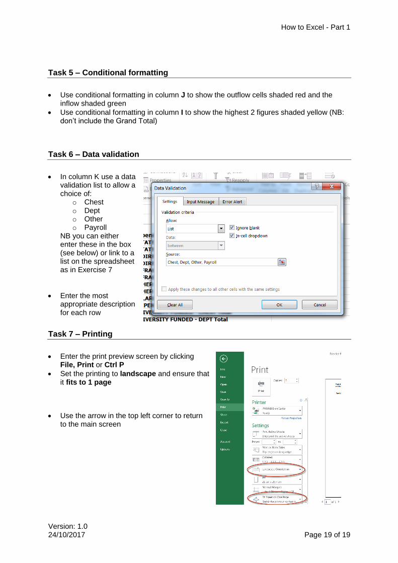
Task 6 – Data validation

In column K use a data validation list to allow a choice of:

o Chest o Dept o Other o Payroll

NB you can either enter these in the box (see below) or link to a list on the spreadsheet as in Exercise 7

Enter the most appropriate description for each row

Task 7 – Printing

Enter the print preview screen by clicking File, Print or Ctrl P

Set the printing to landscape and ensure that it fits to 1 page

Use the arrow in the top left corner to return to the main screen

How to Excel - Part 1 - University of Cambridge · format to Excel (if you haven’t already done...

Documents

Transcript of How to Excel - Part 1 - University of Cambridge · format to Excel (if you haven’t already done...