How Robust is Cason-Plott’s Theory of GameForm Misconception? ∗

Charles Bull† Pascal Courty‡ Maurice Doyon§ Daniel Rondeau¶

January 30, 2016

Abstract

This paper explores the robustness of the theory of game form misconception (GFM)developed by Cason and Plott (2014) to explain bidding mistakes in the Becker-DeGroot-Marschak valuation revelation method. New evidence is broadly consistentwith the existence of two types of bidders and with the presence of bidding noise.However, bidders’ responses to an increase in competition does not accord with GFM.Moreover, we find that misconception increases when subjects perform simultaneouslythe misconceived task and the task it is misconceived for.

Keywords: Game form recognition, subject misconception, mistake, Becker-DeGroot-Marschak, preference elicitation.

JEL Classification: C8, C9.

∗This research was sponsored by the Ministre des Ressources Naturelles du Quebec. The analysis andopinions presented are exclusively those of the authors and errors remain our sole responsibility.†University of Victoria; clbull@uvic.ca.‡University of Victoria and CEPR; pcourty@uvic.ca.§University of Laval; Maurice.Doyon@eac.ulaval.ca.¶University of Victoria; rondeau@uvic.ca.

1 Introduction

Cason and Plott (2014; hereafter CP) argue that experimental subjects sometimes confusethe game they are playing for some other game. They call this type of misconception, gameform misconception (GFM), and argue that it can explain the systematic bidding mistakesfound in the valuation revelation method proposed by Becker-DeGroot-Marschak (Becker etal., 1964; hereafter BDM).1 The purpose of this paper is to test the robustness of the CPtheory of GFM.

CP use a reverse BDM where induced-value cards worth $2 are given to untrained sub-jects. The subjects are instructed to make an “offer price” that, if less than a hidden “postedprice” on the back of the card, would enable them to sell the card for the posted price. If theoffer price turns out to be more than the posted price, the card is redeemed for its value, $2.Consistent with the GFM hypothesis, CP report that some subjects mistakenly believe theyare participating in a first price procurement auction when they are, in fact, participatingin a reverse BDM (which is the same as a second price or Vickrey auction), and conclude:“The subjects consist of at least two groups. One group understands the game form as aa second-price auction and behaves substantially as game theory predicts. Another grouphas a misconception of the game form as a first-price auction and under that model behavessubstantially as game theory predicts.” (p. 1263)

According to CP, misconceived subjects misconceive BDM for a first price auction (FP).Is it correct, however, to assume (as CP do) that misconceived subjects behave like gametheory optimizers in a FP auction? Even more relevant, how do misconceived subjectsbehave when they have to complete both the misconceived task (BDM) and the task it ismisconceived for (FP)? Arguably, one could draw on the large body of experimental evidenceon FP auctions (Kagel and Levin, 1993) to offer speculative answers to these questions.However, CP have warned us that game procedure and context influence game outcomes.This makes cross-game comparisons problematic. More to the point, evidence from FPauctions alone cannot answer the question of how misconception changes when subjects arepresented simultaneously with the misconceived game and the game it is misconceived for.

To test the robustness of the CP theory, we run four distinct experimental treatments: onereplicates the CP’s experiment and the other three modify it to investigate new implicationsof the theory. To start, we compare the data gathered in our replication of CP’s experimentto an experimental first price benchmark rather than a theoretical optimum. Next, weinvestigate whether first price misconceivers respond to an increase in competition as theorypredicts. In that treatment, subjects compete against two posted prices instead of one.Finally, the last treatment explores how bidding behavior changes when subjects are askedto perform both the misconceived task (BDM) and the task it is misconceived for (first price)simultaneously.

Our results show support for CP’s theory of subject misconception general premise thatsubjects are composed of two groups that behave significantly differently. However, we show

1Understanding the nature of such mistake is important to interpret revealed preferences in the BDMvaluation method: ‘’It is a failure of the decision maker to recognize the proper connections between the actsavailable for choice and the consequences of choice, which, by necessity, are associated with the method ofmeasuring preferences. If the individual fails to understand the connection between acts and outcomes, thechoice of acts can be misleading about the preferences over outcomes.” (p. 1237)

1

that the group of first price misconceives does not respond to an increase in competition ina BDM payment mechanism as optimizing behavior under game theory predicts. We alsofind that presenting simultaneously the misconceived task and the task it is misconceivedfor surprisingly increases, rather than decreases, misconception.

Section 2 reviews CP’s theory of GFM. Section 3 describes the experimental design andgoes over the procedures used during the experiment. Section 4 provides an overview of thedata gathered, replicates CP results and presents evidence that some subjects misconceivethe payment method used to compute payoffs. Although some of the treatments include asecond ‘repeat’ round, we discuss the evidence on the second round only in the replicationof CP analysis. Section 5 presents the main results of this paper and Section 6 summarizesthe main findings. The Appendix, presents further analysis and details on the experimentaldesign.

2 CP’s Theory of GFM: The BDM Case

The BDM is an incentive–compatible procedure for measuring a subject’s WTA or WTP.2

Standard economic theory implies that for a given object, a subject’s WTP should be equalto their WTA (i.e., the most one is willing to pay for an object is equal to the lowest priceone is willing to sell the same object for). Several experiments using the BDM, however,have found that many subjects state a greater WTA than WTP and have attributed thisdifference to a behavioral bias (the literature refers to the notions of ‘endowment effect’,framing, reference point and loss aversion).3 Plott and Zeiler (2005) dispute this popularconclusion and instead argue for the possibility that subjects have misconceptions.4 In theiroverview of the literature on WTA-WTP gaps, they note that “experimenters are carefulto control for subject misconceptions, [but] there is no consensus about the fundamentalproperties of misconceptions or how to avoid them. Instead, by implementing different typesof experimental controls, experimenters have revealed notions of how misconceptions arise”(p. 530).5

CP focus on a specific type of misconception in an induced-value experiment, thus elim-inating unobserved preferences. Subjects are given a card and are told that they can sellit for $2. According to CP “all theories agree that the preference value the subjects placeon the card is $2.” Since induced-value cards are used instead of goods, the only matter to

2Karni and Safra (1987) showed that this does not follow if the good in question is a lottery and Horowitz(2006) shows that this result need not be true for non-expected utility maximizers.

3See Plott and Zeiler (2005) Table 1 for an overview of experimental papers on WTA-WTP gaps.4They report “while many experimenters have observed a WTP-WTA gap, others have failed to observe

it. This variation in experimental results seriously undermines the claim that the gap is a fundamentalfeature of human preferences” (p. 531).

5Procedures used to control for subject misconception include using an incentive-compatible elicitationdevice, subject training, paid practice rounds, and the provision of anonymity for subjects. Plott and Zeiler(2005) first replicate a prominent experiment in the literature cited as evidence for the endowment effect,Experiment 5 in Kahneman et al. (1990), and then proceed to implement all possible controls for subjectmisconception found in the literature. WTA-WTP gaps were noted in the former but not the latter, providingevidence that the particular experimental procedures, not the endowment effect, are responsible for the notedgaps. However, Bartling, Engl, and Weber (2014) show that framing effects, such as the endowment effect,can persist in trained subjects that show correct game form recognition.

2

study is why, in the absence of training or explanation of the BDM rules, some subject biddifferent amounts than $2.

CP argue that the reason some subjects make systematic mistakes is because they donot understand the game they are playing. They question the implicit assumption made inmany experimental studies that there necessarily exist “a solid connection between the gameform and an individuals understanding of the game form.” They acknowledge that theremay be many forms of misconception, but they argue that a significant fraction of mistakesin a BDM game can be attributed as subjects misconceiving the BDM auction as a first price(FP) auction, a mistake they call Game Form Misconception (GFM): “The mistakes are notsimply random departures from a correct understanding of the experimental task, but ratherarise from a misconception of the rules of the BDM.” They take the next step and arguethat an experimenter who knows the game that is misconceived as the game being playedcan make prediction on how the subject should respond to changes in game parameters: “Inorder to make a case that the choices reflect a systematic, fundamental mistake, the mistakeitself is described and stated in a form that yields testable predictions that are comparableto the predictions of other possible models.” To summarize, CP’s application of GFM theoryto interpret bidding outcomes in a BDM is based on the following three premises:

Premiss 1. Subject heterogeneity: some subjects are BDM optimizers and others have GFM.

CP write, “The data are better and more completely explained by a mixture of somesubjects who understand the BDM mechanism and submit optimal offers and others whohave a specific type of game form misconception.”

Premiss 2. GFM applies to BDM but not to FP.

According to CP, “The choices of many of these untrained subjects appear to be basedon a misconception of the task. They think that it is a first-price auction rather than asecond price auction.” (p. 1262). Thus, subjects with GFM behave in BDM as if they werein a FP auction. This establishes testable predictions on how misconceived subjects shouldrespond when the parameters of the BDM game changes. They should respond as if thegame rules were FP because a misconceived subject “has a misconception of the game formas a first-price auction and under that model behaves substantially as game theory predicts.”CP also argue that subjects make random decision errors.

Premiss 3. Subjects bid distribution is best explained with random decision noise.

CP consider models of optimal decision with noise because: “Mistakes, decision error,and noise can complicate inferences about fundamental economic primitives, and these com-plications call for stochastic and heterogeneous models.”

Using these three premises, CP explain experimental data on variations of the BDMusing induced-value cards. This paper first replicates most of their results and subsequentlymoves on to develop new variations of the BDM to further test CP theory of GFM.

3 Experimental Design

The experiment performed in this study consists of four similar, though distinct, treatments.In all of the treatments, subjects were given two cards worth $2 each and were informed of a

3

rule by which they could sell them back to the experimenter. In the first three treatments,subjects are given two cards sequentially. In the last treatment, subjects are given 2 cardssimultaneously.

3.1 BDM and First Price Treatments

Subjects performed two rounds of these treatments, though the second was unannounced.Each subject was handed a large envelope that contained detailed instructions on how toperform the experiment; an experiment card; a consent form; and a smaller envelope. Afterthe subjects completed the experiment card, the instructions prompted them to open thesmaller envelope. Inside the smaller envelope was a second experiment card that used thesame sale mechanism. Subjects were instructed to complete this card and put all the material,except for a tag with an ID number on it, back in the large envelope. This tag was theirticket for payment. Payments to subjects were made in subsequent lab sections and lectures.

3.1.1 CP Replication (BDM1)

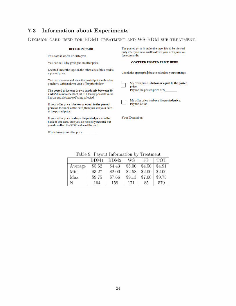
The BDM1 treatment uses a reverse BDM sale mechanism. The subject is instructed to readthe card over and write down an offer price. On the back side of the experiment card is acovered posted price randomly drawn from the distribution U(0,5); subjects are instructedto uncover the posted price only after writing down an offer price. If their offer price is lessthan or equal to the posted price, the subject sells their experiment card at the posted price.If their offer price is greater than the posted price, the subject sells their card for $2.Thetheoretically optimal offer for an expected utility maximizer only concerned with monetarypayoffs is $2.

BDM1 more or less replicates the experiment performed in CP. As in CP, this treatmentconsists of two rounds. The wording on the card was slightly edited for clarity. An importantdistinction with CP is that subjects are told that all posted prices would be drawn from auniform distribution with support [0, 5]—a fact made known to subjects in plain English (seeAppendix for an example experiment card). Moreover, we use a single price distribution forall groups while CP use different distributions of posted prices with different groups.

3.1.2 First Price (FP)

The FP treatment uses a first price sale mechanism. The subject is instructed to read thecard over and write down an offer price. On the back side of the experiment card is a coveredposted price randomly drawn from a uniform distribution with support [0, 5]; subjects areinstructed to uncover the posted price only after writing down an offer price. Subjects areinformed in plain English about the distribution the posted prices are drawn from. If theiroffer price is less than or equal to the posted price, the subject sells their experiment cardat their offer price. If their offer price is greater than the posted price, the subject sells theircard for $2.

The optimal offer price for a risk neutral subject is $3.50 in this treatment (given thatthe random price is uniform with support [0, 5]). The first round of FP is referred to as FP1,and the second round is referred to as FP-2.

4

Our main critique of CP’s analysis is that the modeling technique they employed com-pares experimental behavior in the BDM to theoretical optimizing BDM and first pricebehavior. Our motivation for including the FP treatment is to provide a behavioral firstprice benchmark to compare with our replication of CP’s experiment (BDM1), as subjectsparticipating in first price auctions tend not to act according to what game theory predicts(Harrison, 1990).

3.1.3 Increased Competition (BDM2)

The BDM2 treatment differs from BDM1 in one way: two posted prices are drawn, not one.The subjects are instructed that if their offer price is less than both posted prices, or equalto the lowest posted price, they sell their experiment card at the posted price. If their offerprice is greater than one or both of the posted prices, they sell their experiment card for $2.The subject is informed in plain English that both posted prices are randomly drawn fromthe distribution U(0,5). An offer price of $2 is again optimal. The first round of BDM2 isreferred to as BDM2-1, and the second round is referred to as BDM2-2.

Our motivation for including this treatment in the experiment is to observe the behaviorof CP’s so-called first price misconceivers. As optimal first price behavior changes with thenumber of bidders, a good test of CP’s theory would be to vary the number of posted prices.If a group of first price misconceivers is indeed present, and of any meaningful size, the offerdistribution of BDM2 should differ from that of BDM1 in key areas. Most notably, the offerdistribution should be shifted to the left relative to that of BDM1’s. It should also containa statistically greater amount of offers around $3.00 (the optimal offer for BDM2 under thefirst price misconception model).

3.2 Simultaneous Task Completion (Within Subject — WS)

The WS (within–subject) treatment presents the subject with two experiment cards fromthe outset. One of the cards uses the mechanism found in BDM1, and the other usesthe mechanism found in FP. The subjects are notified by the instructions that the salemechanisms are different, though the subjects must discern the difference themselves. Thecard using the BDM sale mechanism is referred to as WS-BDM, while the card using thefirst price sale mechanism is referred to as WS-FP.

We include this treatment in our experiment to observe the behavior of subjects whenconfronted with a BDM and a FP mechanism simultaneously. By explicitly telling subjectsthat the two cards implement different payment mechanisms, we expect a greater proportionof them to correctly recognize the games they are playing and thus move the bid distributionstowards their respective optima.

Copies and examples of all material used during the experiment (instructions, consentforms, experiment cards) can be found in the Appendix.

3.3 Procedures

Experimental sessions lasted approximately twenty-five minutes and were run in first–yearundergraduate classes at the University of Victoria. Subjects were not trained and were told

5

that the purpose of the research project was to understand how participants take advantageof simple trading opportunities in different forms.

All experimental material was prepackaged in envelopes and handed out in an alternatingpattern, ensuring that each treatment’s envelopes was homogeneously distributed across theentire classroom (a fact made known to the subjects). For every envelope of FP handed out,two envelopes of BDM1, BDM2, and WS were each handed out. Subjects were instructednot to talk to one another until the experiment was completed. Very few instances of talkingwere noted by proctors. All data were gathered in arena-style classrooms: 235 participated inthe first session, 309 in the second, and 36 in the third. A total of 579 subjects participated:164 in BDM1, 159 in BDM2, 171 in WS, and 85 in FP. In the first two sessions the subjectto proctor ratio was roughly 30:1; in the third it was 18:1. The data were collected over theperiod September 22-23, 2015. The experiment was run using Canadian dollars.

Of the 164 subjects that participated in BDM1, 163 completed both experiment cards;158 of the 159 subjects that participated in BDM2 completed both experiment cards; 170 ofthe 171 subjects that participated in WS completed both experiment cards; and 83 out of85 of the subjects that participated in FP completed both experiment cards. It is unknownwhy five subjects only completed one of the two cards presented to them; however, the datathey provided is used when appropriate.

Subjects were informed they could earn up to $10. The average payout was $4.91, theminimum was $2, and the maximum was $9.75. Table 9 in the Appendix breaks down payoutresults by treatment.

For convenience of both the experimenters and the subjects, payouts were rounded up tothe nearest quarter dollar. Subjects were not aware of the rounding up at the time of theexperiment. Cards handed back without being filled out were considered given back and notsold; consequently payment was not made on them.

4 Data, CP Replication, and Revealed Misconceptions

Table 1 presents summary descriptive statistics for all four treatments. We refer to thattable throughout the rest of this paper. Each treatment is broken down into two sub-treatments, which correspond to a repetition of the task for the first three treatments andto the two distinct tasks done simultaneously in the last treatment. Table 1 first presentssimple statistics on the distribution of bids and then computes the fraction of offers measuredat key points in the distribution that correspond to the optimal offers under three auctionrules ($2 for all BDM, $3.5 for FP with one random bid and $3 for FP with two randombids). The table also reports the fraction of outliers bids (offers below $.10 and above $5).The bottom part of the table reproduces results on misconception regarding the rule usedto compute payoffs as defined in CP, and discussed in section 4.2.

6

4.1 CP Replication

CP provide five main results in Section V of their paper. Our data allows to test four ofthese results (Results 1, 2, 3, and 5).6 We compare our baseline findings in BDM1 withthese four results. When relevant, we also discuss results from BDM2 keeping in mind thatthis treatment differs from CP treatments in that subjects compete against two random bidsinstead of one. Detailed information can be found in the Appendix.

CP 1. With simple instructions and no training or feedback, the BDM does not providereliable measures of preferences for the induced-value object.

In BDM1-1, 7.9% of subjects offer within 5 cents of $2 while in BDM2-1, 8.8% of subjectsoffer with 5 cents of $2. The corresponding number in CP is higher 16.7%.

CP 2. A second round of decisions (including subjects rereading the instructions and afterreceiving feedback) nearly doubles the number of subjects stating the correct valuation.

The fraction of subjects offering amounts within 5 cents of $2 increases to 13.5% inBDM1-2 and 13.3% in BDM2-2. Fisher’s exact test gives p-values of 11.1% and 21.5%,respectively, indicating that this is not a statistically significant shift in either treatment.However, the difference in statistical significance may be explained by the fact that we testthis hypothesis using BDM1 and BDM2 samples (about 160 subjects each) while CP usetheir entire sample pooling different sub-treatments (244 subjects). In fact, when we poolBDM1 and BDM2 treatments (which is similar to CP pooling data from sub-treatments withdifferent supports for the random price), the increase across rounds in the fraction of offerswithin 5 cents of $2, is significant (the Fishers exact test gives a p-value of 0.0432).

CP 3. Subjects that chose the theoretically optimal offer price (near $2) on the first cardalso usually choose the theoretically optimal offer price on the second card. Subjects who didnot choose optimally on the first card tend to choose a different offer price on the secondcard.

Take BDM1 where 163 subjects completed both cards. Out of these subjects, 13 offereda bid within 5 cents of $2 in BDM1-1. Of these 13 subjects, 76.9% offered the same amountin BDM1-2. Of the 150 subjects who did not offer within 5 cents of $2, 79.3% offered adifferent amount in BDM1-2. As put in CP “The hypothesis that the stability of choiceis the same for those who chose optimally and those who did not choose optimally on thefirst card is strongly rejected” (p. 1248) (Fisher’s exact test p-value < 0.001). These resultsextend when we compare stability of choice across BDM2-1 and BDM2-2 (Fisher’s exact testp-value < 0.002).

CP 5. Subjects who were “exposed” to their mistake (in the sense that a different offeramount would have increased their payoff) were more likely to choose a correct offer inround 2.

6We cannot investigate Result 4 because we have used a single upper-bound ($5) for the support of therandom price in our treatments.

7

In BDM1, exposed subjects are more likely to move toward the optimum (bid within5 cents of $2) than non-exposed ones. They are also less likely to move away from theoptimum. Both these results are statistically significant. However, exposed subjects are notmore likely to move onto the optimum. For BDM2, exposed subjects are more likely to movetoward the optimum. See explanations and Tables 6 and 7 in the Appendix for a completebreakdowns of these results.

To sum up, we conclude that our results largely agree with CP’s main findings:

Result 1. Results 1-3 and 5 from CP are replicated with similar quantitative effects andstatistical significance.

This validation of CP’s findings establishes a solid ground for the interpretation of thenew treatments that follow.

4.2 Revealed Misconception

Folllowing CP, we say that a subject has first price misconception (FPM) in a given BDM sub-treatment (BDM1-1, BDM1-2, BDM2-1, BDM2-2, and WS-BDM) if she wins and requeststo be paid her offer price instead of the posted price. By symmetry, we say that a subjecthas second price misconception (SPM) in a FP sub-treatment (FP and WS-FP) if she winsand asks to be paid the posted price instead of her offer price. Revealed misconceptions areerrors in the reported payment requested by subjects. Although these mistakes do not affectpayoffs, they reveal something about subjects’ understanding about the rule used to computepayoffs. As in CP, we use the term possible misconception to refer to the instances in whicha subject may or may not have had a misconception, but could not reveal it as she did notwin in either round (her offer price was less than the posted price in both sub-treatments).

The lower part of Table 1 presents evidence on FPM and SPM. As a benchmark, CPreport that 11.8% of subjects explicitly revealed a misconception on the experiment card(i.e., they asked to be paid their offer price, not the posted price when the posted price isgreater than their offer price). The corresponding FPM rate in BDM1 is 13.4%. As thesenumbers accord quite well, it can be assumed that a group of first price misconceivers, similarin relative size to that in CP, is present in our data. The proportion of subjects possiblyharboring FPM in BDM1 is 31.1%—this number is 33.5% in CP. The BDM1 misconceptionrate accords well with the misconception rate present in CP, providing evidence that a groupof first price misconceivers, as defined in CP, is present and of similar size in our dataset.

The rate of FPM varies over the different sub-treatments. Ex ante we hypothesized theWS treatment would reduce the rate of FPM. It did not. The rate of FPM in WS-BDM,9.9%, is not statistically different from that in BDM1-1, 6.1%. The similar misconceptionrates in BDM1-1 and WS-BDM indicate that confronting subjects with both mechanismssimultanenously (that is, giving information on FP in addition to BDM), does not affectFPM.7

Result 2. Revealed misconception is found only for BDM (not for FP) when subjects performa single task. Revealed misconception increases and is even found in the FP task when

7Subjects make fewer FPM in payoff computation in BDM2: we have 1.9% FPM out of 34% who won atleast one card instead of 13.5% versus 69.9% in BDM1.

8

subjects have to perform simultaneously the misconceived task and the task it is misconceivedfor.

The rate of SPM in WS-FP, 7.6%, is statistically greater than that in FP1, 1.2%. Unlikethe instances of FPM which were expected, the instances of SPM were a surprise. If onetreats the SPM rate in FP1, 1.2%, as the baseline SPM rate, the subjects we define as secondprice misconceivers in WS-FP (7.6%) may in fact be the result of a treatment effect. In otherwords, seeing both payment mechanisms confused, rather than helped these subjects!

5 Results: BDM, First Price and Competition

The rest of the paper focuses on the first rounds of BDM1, BDM2, FP and on the WS treat-ment. We compare five sub-treatments: BDM1-1, BDM2-1, FP1, WS-BDM and WS-FP.We repeatedly refer to Tables 2, 3, and 4 which provide various tests of equality regardingdifferent features of the distributions in these five sub-treatments. Table 2 provides resultsof variance ratio tests, which test the equality of variances across the sub-treatments; Table3 shows the results of Mann-Whitney U-tests, which test whether two independent samplescome from populations with the same distribution; and Table 4 reports the results of Pear-son’s chi-squared tests, which test whether the two samples came from distributions withthe same median.8

5.1 First Price Auction (FP1)

Premiss 2 in CP theory says that subjects do not harbor GFM for FP. This premiss isconsistent with the experimental literature on first price auctions which has not reportedsystematic bias in bidder strategy (Kagel and Levin, 1993). CP, however, have also warnedus that game procedures can influence misconception in general and GFM in particular.Thus, experiment FP1 is a control experiment that holds constant all game procedure. Theenvironment is identical to BDM1 in all respect but the auction rule used to determinedpayoffs.

Result 3. The distribution of bids in FP1 is consistent with subjects bidding the theoreticalrevenue maximizing bid of $3.5 with noise.

This finding is consistent with Premisses 2 and 3. The observation that subjects computetheir payoff properly (no SPM in Table 1) also supports the conclusion that GFM does notapply to FP1 even after controlling for all game procedure.

5.2 Comparison of BDM1-1 and FP1

We look at the similarities and differences in the distributions of first round offers of theBDM1 and FP treatments. A quick look at Table 1 shows that the mean of FP1 is higherthan that of BDM1-1. Moreover, all tests of distribution similarity are rejected at the 5%

8Mann-Whitney U-tests and Pearson’s chi-squared tests are used rather than t-tests, as treatment dataare not normally distributed.

9

significance level, except the variance ratio test. The two raw distributions of offers appearto be statistically different. Subjects bid more in FP resulting in the distribution of bids inFP1 stochastically dominating the distribution of bids in BDM1-1.

Result 4. Subjects bid more in FP1 than in BDM1-1

This is consistent with CP interpretation of BDM1-1 bids. There are two types of bidders:theoretical BDM and subjects that misconceive BDM for FP. FP1, however, has only FPbidders. Since FP bidders bid more than the theoretical BDM optimum bid, we would expectthe FP1 bid distribution to stochastically dominate the BDM1-1 bid distribution.

The optimal bid for non-misconceived subjects is $2 in BDM1-1. About 7.9% of thesubjects of bids around $2 in BDM1-1. CP conjectured that these subjects must be BDMoptimizers. However, we find a similar fraction of bids around $2 in FP1. Indeed, theproportion of offers within 5 cents of $2 is statistically indistinguishable in BDM1-1 andFP1 (proportions test p-value = 0.9323).

Result 5. The fraction of subjects that bids near $2 is the same in BDM 1-1 and FP1.

The proportions of subjects offering within 5 cents of $2 in both sub-treatments is sta-tistically the same, indicating that those bids within 5 cents of $2 in BDM1-1 may not beBDM optimizers as conjectured by CP.9 It is not possible to associate bids of $2 in BDMas correctly optimized BDM bids because we observe a similar fraction of bids of $2 in FP.These bids are also consistent with the noise associated with FP bids. This qualifies CP’schoice to classify $2 bid as BDM optimizers and calls for care in interpreting these bids.

Another type of misconception is present in BDM1-1. There are six offers below 10 centsin BDM1-1, and zero of such offers in FP1. A low offer in the BDM represents a specifictype of misconception in which the subjects ensure they will be able to sell their card, butdo not process that the random draw could be between $0 and $2. The proportions of offersless than 10 cents are statistically different at the 10% level of significance, but not at the5% level of significance.

5.3 Competition: BDM1-1 versus BDM2-1

The purpose of including the BDM2 treatment is to inspect the response of CP’s first pricemisconceivers to a change in game parameter. The optimal offer in BDM2-1 is $2—just asin BDM1 and WS-BDM; however, the optimal offer under first-price misconception is $3.00,not $3.50 as in BDM1-1. This is because of the addition of a second random price calls for amore aggressive bid. According to Premiss 2, the group of misconceivers should respond tothis change in game parameter. As a result, one would expect the BDM2-1 bid distributionto shift to the left relative to that of BDM1-1.

Result 6. Subjects do not bid less when there is an additional random price.

The mean of BDM2-1 is $3.27, higher than that of BDM1-1, $2.93. The medians andmodes of the distributions are both equal to $3.00. The mean and median of the BDM2-1

9The same conclusion holds if we look at BDM2-1 instead. The proportions of offers within 5 cents ofthe optimum in BDM1-1 and BDM2-1 are practically the same, 7.9% and 8.8%, respectively.

10

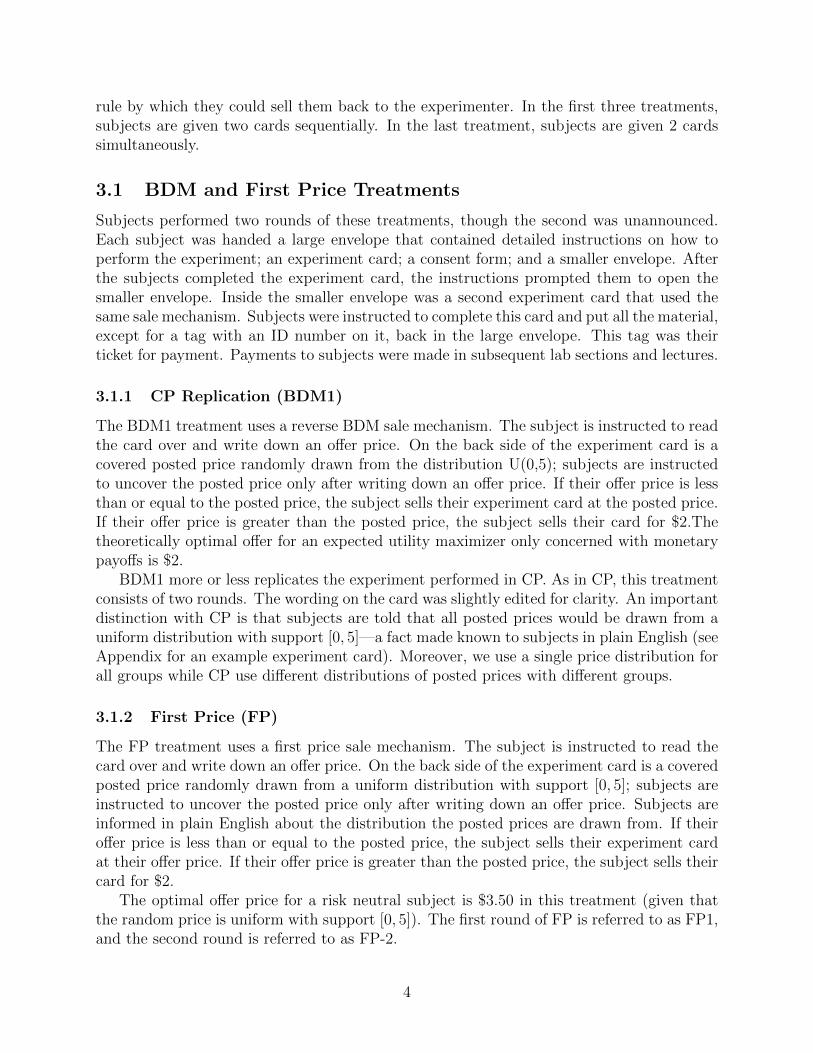
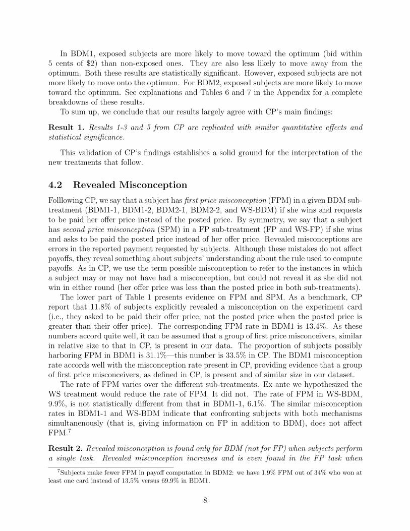
bid distribution are not lower relative to those of the BDM1-1 bid distribution. Figure 1shows the CDFs for BDM1-1 and BDM2-1 graphed one upon another. When comparingBDM1-1 and BDM2-1s distributions, Mann-Whitney’s two sample U-test provides a p-valueof 5.9%, while Pearson’s chi-squared test provides a p-value of 21%. A variance ratio testshows that at the 1% level of significance, the two samples have different variances. There isclearly some evidence for, and some evidence against, these samples coming from the samedistribution.

The same conclusion holds if we look instead at the proportions of offers within 5 cents of$3.00, 26.2% in BDM1-1 and 20.1% in BDM2-1. These figures are not statistically differentfrom one another (proportions test p-value = 0.1947), casting doubt on CP’s claim that agroup of subjects harboring a first price misconception, but otherwise behaving substan-tially as game theory predicts, actually exists. If this group were to exist, and was of anymeaningful size, there would be a statistically greater proportion of offers within 5 cents of$3.00 in BDM2-1 than BDM1-1. This is not the case. It is also of interest to note thatthe proportions of offers within 5 cents of $3.50 are statistically indistinguishable in bothBDM1-1 and BDM2-1 at all conventional levels of significance.

Experimental evidence from FP auctions shows that bidders respond to the number ofbidders by putting more aggressive (lower in our experiment) bids as predicted by theory(Kagel and Levin, 1993). However, we reject the prediction that GFM subjects respond toand increase in competition (decrease their offer with an additional bidder.) Misconceptiondoes not carry through for this auction dimension. Based on this alone, the hypothesis thatmisconceived BDM bidders behave like FP optimizers is squarely rejected.

This finding must be constrasted with CP Result 4. CP have four sub-treatments. Inthese sub-treatments, the range of of the random price is [0, p] and p take values 4, 5, 6, 7, 8.The optimal FP bid is 1 + 0.5p. Thus, varying p by one unit, as CP do in Result 4, isequivalent to increasing the number of random offers from one to two, as we do in BDM2.The point is that CP vary a game parameter (upper bound of random price) that asks for thesame FP response as the game parameter we vary (number of random offers). The averageoffer increases almost monotically with p across sub-treatments and this is despite the factthat they have relatively few observations in each subtreatment (about 40). In contrast, wefind no response to an increase in competition when we increase the number of bidders (andwe have about 160 subjects in each sub-treatment). To conclude, our result is not due tohaving a small sample and it is not due either to measuring too small a potential response.

5.4 Simultaneous Task Completion (WS)

In the WS treatment, we present the BDM and FP tasks simultaneously. The only differencebetween the BDM1-1 (FP1) card and the WS-BDM (WS-FP) card is that the WS cards werepresented together. We included this treatment to inspect the behavior of subjects whenconfronted with both payment mechanisms. Seeing the WS-FP (WS-BDM) card may haveinfluenced the offers made in WS-BDM (WS-FP). Explicitly telling subjects that the twocards implement different mechanisms could have two effects. If comparing informationhelps subjects understanding the two tasks, we would expect them to consider differentstrategies in both sub-treatments which would drive the distributions apart, toward theirrespective optima. Alternatively, doing both task together may increase confusion. Subjects

11

have to absorb and process more information. This increase in complexity may lower taskcomprehension and increase GFM.

Result 7. When subjects are asked to complete both BDM and FP tasks simultaneously,bidding strategies do not differ across tasks.

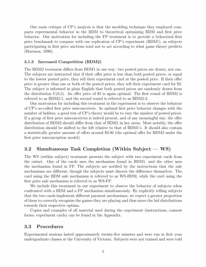
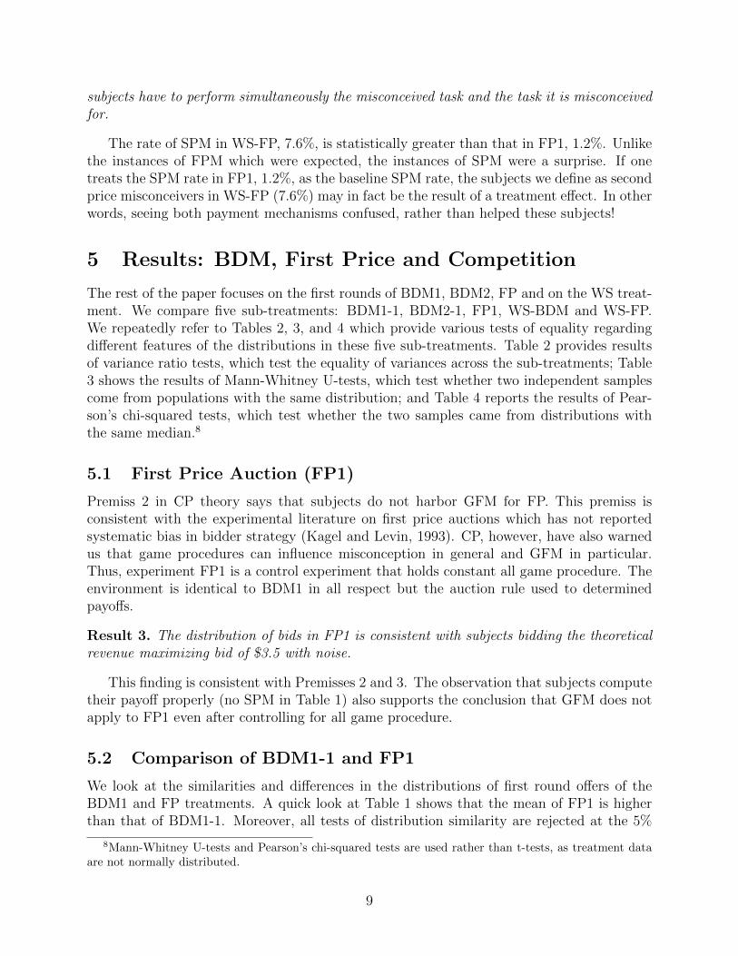
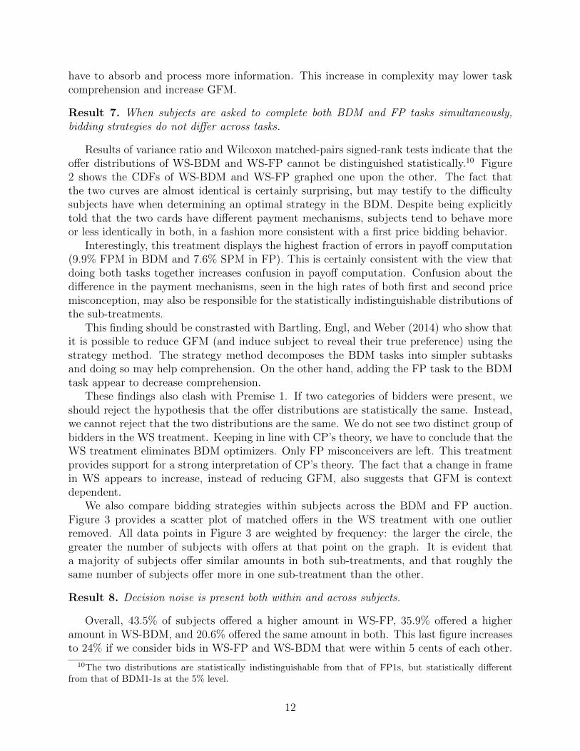
Results of variance ratio and Wilcoxon matched-pairs signed-rank tests indicate that theoffer distributions of WS-BDM and WS-FP cannot be distinguished statistically.10 Figure2 shows the CDFs of WS-BDM and WS-FP graphed one upon the other. The fact thatthe two curves are almost identical is certainly surprising, but may testify to the difficultysubjects have when determining an optimal strategy in the BDM. Despite being explicitlytold that the two cards have different payment mechanisms, subjects tend to behave moreor less identically in both, in a fashion more consistent with a first price bidding behavior.

Interestingly, this treatment displays the highest fraction of errors in payoff computation(9.9% FPM in BDM and 7.6% SPM in FP). This is certainly consistent with the view thatdoing both tasks together increases confusion in payoff computation. Confusion about thedifference in the payment mechanisms, seen in the high rates of both first and second pricemisconception, may also be responsible for the statistically indistinguishable distributions ofthe sub-treatments.

This finding should be constrasted with Bartling, Engl, and Weber (2014) who show thatit is possible to reduce GFM (and induce subject to reveal their true preference) using thestrategy method. The strategy method decomposes the BDM tasks into simpler subtasksand doing so may help comprehension. On the other hand, adding the FP task to the BDMtask appear to decrease comprehension.

These findings also clash with Premise 1. If two categories of bidders were present, weshould reject the hypothesis that the offer distributions are statistically the same. Instead,we cannot reject that the two distributions are the same. We do not see two distinct group ofbidders in the WS treatment. Keeping in line with CP’s theory, we have to conclude that theWS treatment eliminates BDM optimizers. Only FP misconceivers are left. This treatmentprovides support for a strong interpretation of CP’s theory. The fact that a change in framein WS appears to increase, instead of reducing GFM, also suggests that GFM is contextdependent.

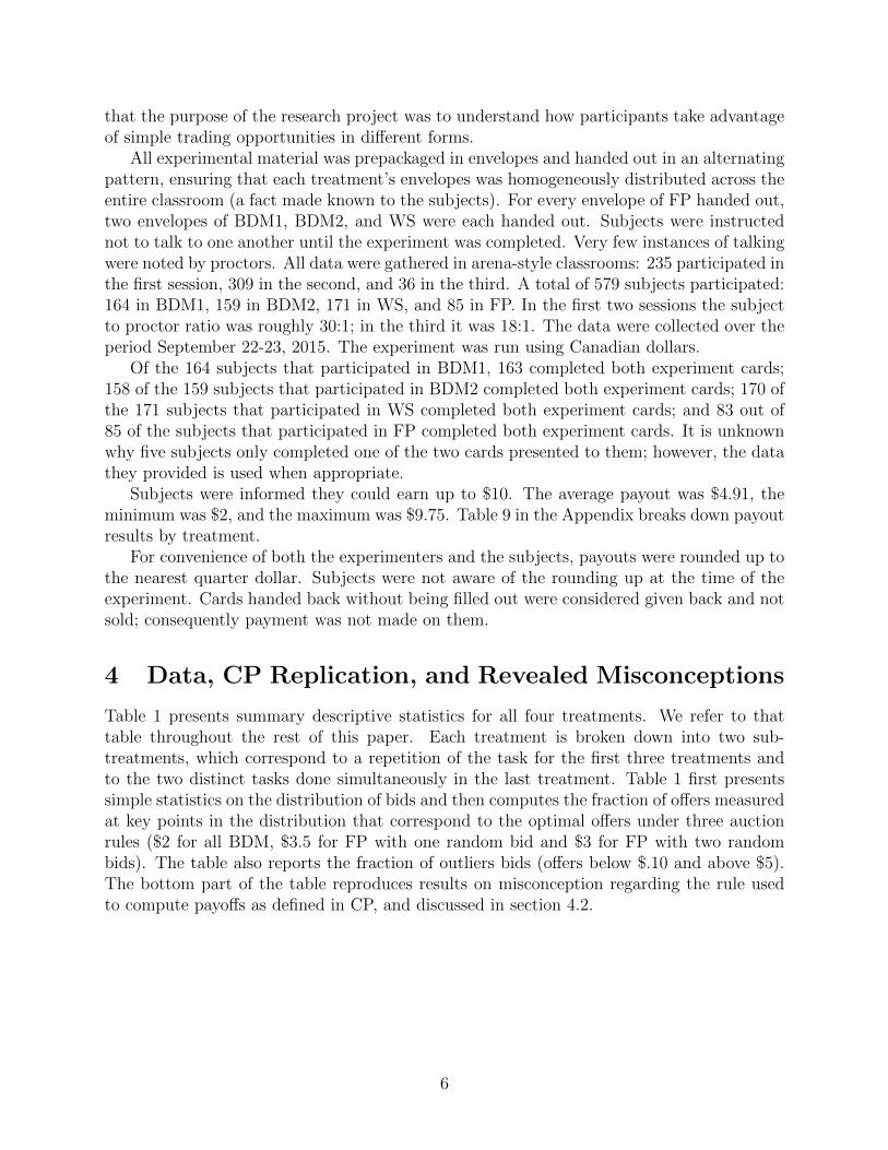
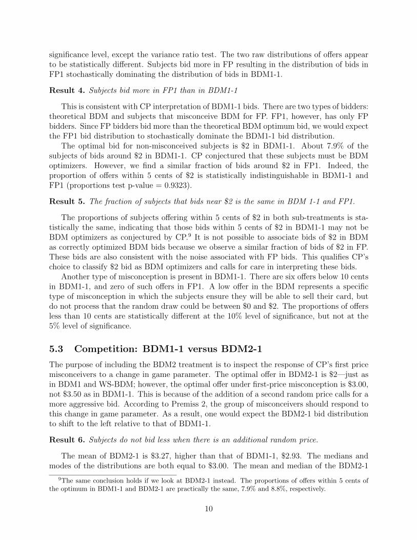
We also compare bidding strategies within subjects across the BDM and FP auction.Figure 3 provides a scatter plot of matched offers in the WS treatment with one outlierremoved. All data points in Figure 3 are weighted by frequency: the larger the circle, thegreater the number of subjects with offers at that point on the graph. It is evident thata majority of subjects offer similar amounts in both sub-treatments, and that roughly thesame number of subjects offer more in one sub-treatment than the other.

Result 8. Decision noise is present both within and across subjects.

Overall, 43.5% of subjects offered a higher amount in WS-FP, 35.9% offered a higheramount in WS-BDM, and 20.6% offered the same amount in both. This last figure increasesto 24% if we consider bids in WS-FP and WS-BDM that were within 5 cents of each other.

10The two distributions are statistically indistinguishable from that of FP1s, but statistically differentfrom that of BDM1-1s at the 5% level.

12

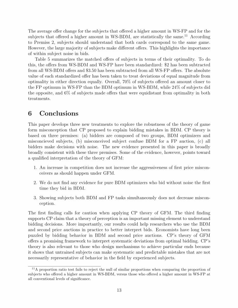
The average offer change for the subjects that offered a higher amount in WS-FP and for thesubjects that offered a higher amount in WS-BDM, are statistically the same.11 Accordingto Premiss 2, subjects should understand that both cards correspond to the same game.However, the large majority of subjects make different offers. This highlights the importanceof within subject noise in bids.

Table 5 summarizes the matched offers of subjects in terms of their optimality. To dothis, the offers from WS-BDM and WS-FP have been standardized: $2 has been subtractedfrom all WS-BDM offers and $3.50 has been subtracted from all WS-FP offers. The absolutevalue of each standardized offer has been taken to treat deviations of equal magnitude fromoptimality in either direction equally. Overall, 70% of subjects offered an amount closer tothe FP optimum in WS-FP than the BDM optimum in WS-BDM, while 24% of subjects didthe opposite, and 6% of subjects made offers that were equidistant from optimality in bothtreatments.

6 Conclusions

This paper develops three new treatments to explore the robustness of the theory of gameform misconception that CP proposed to explain bidding mistakes in BDM. CP theory isbased on three premises: (a) bidders are composed of two groups, BDM optimizers andmisconcieved subjects, (b) misconceived subject confuse BDM for a FP auction, (c) allbidders make decisions with noise. The new evidence presented in this paper is broadlybroadly consistent with these three premises. Some of the evidence, however, points towarda qualified interpretation of the theory of GFM:

1. An increase in competition does not increase the aggressiveness of first price miscon-ceivers as should happen under GFM.

2. We do not find any evidence for pure BDM optimizers who bid without noise the firsttime they bid in BDM.

3. Showing subjects both BDM and FP tasks simultaneously does not decrease miscon-ception.

The first finding calls for caution when applying CP theory of GFM. The third findingsupports CP claim that a theory of perception is an important missing element to understandbidding decisions. More importantly, our results could help researchers who use the BDMand second price auctions in practice to better interpret bids. Economists have long beenpuzzled by bidding behavior in BDM and second price auctions. CP’s theory of GFMoffers a promising framework to interpret systematic deviations from optimal bidding. CP’stheory is also relevant to those who design mechanisms to achieve particular ends becauseit shows that untrained subjects can make systematic and predictable mistakes that are notnecessarily representative of behavior in the field by experienced subjects.

11A proportion ratio test fails to reject the null of similar proportions when comparing the proportion ofsubjects who offered a higher amount in WS-BDM, versus those who offered a higher amount in WS-FP atall conventional levels of significance.

13

References

Kagel, J. H., and D. Levin. 1993. Independent private value auctions: Bidder behaviour infirst-, second-and third-price auctions with varying numbers of bidders. The EconomicJournal :868–879.Bartling, B., Engl, F., & Weber, R. A. (2014). Game form misconceptions do not explain

the endowment effect. CESifo Working Paper Series No. 5094. Available at SSRN:http://ssrn.com/abstract=2536297.

Becker, G. M., DeGroot, M. H., & Marschak, J. (1964). Measuring utility by a singleresponse sequential method. Behavioral Science, 9 (3), 226-232.

Benartzi, S., & Thaler, R. H. (2007). Heuristics and biases in retirement savings behavior.The Journal of Economic Perspectives, 21 (3), 81-104.

Binmore, K.,& Samuelson, L. (1994). An economist’s perspective on the evolution ofnorms. Journal of Institutional and Theoretical Economics (JITE)/Zeitschrift furdie gesamte Staatswissenschaft, 45-63.

Cason, T. N., & Plott, C. R. (2014). Misconceptions and game form recognition: Chal-lenges to theories of revealed preference and framing. Journal of Political Economy,122 (6), 1235-1270.

Cooper, D. J., & Fang, H. (2008). Understanding overbidding in second price auctions:An experimental study*. The Economic Journal, 118 (532), 1572-1595.

Goeree, J. K., Holt, C. A., & Palfrey, T. R. (2002). Quantal response equilibrium andoverbidding in private-value auctions. Journal of Economic Theory, 104 (1), 247-272.

Harrison, G. W. (1990). Risk attitudes in first-price auction experiments: A Bayesiananalysis. The Review of Economics and Statistics, 72 (3), 541-546.

Heitjan, D. F. (1989). Inference from grouped continuous data: a review. StatisticalScience, 4 (2) 164-179.

Horowitz, J. K. (2006). The Becker-DeGroot-Marschak mechanism is not necessarilyincentive compatible, even for non-random goods. Economics Letters, 93 (1), 6-11.

Kahneman, D., Knetsch, J. L., & Thaler, R. H. (1991). Anomalies: The endowmenteffect, loss aversion, and status quo bias. The Journal of Economic Perspectives,5 (1) 193-206.

Kahneman, D., Knetsch, J. L., & Thaler, R. H. (1990). Experimental tests of the endow-ment effect and the Coase theorem. Journal of Political Economy, 98 (6),1325-1348.

Karni, E., & Safra, Z. (1987). “Preference reversal” and the observability of preferencesby experimental methods. Econometrica: Journal of the Econometric Society, 55 (3),675-685.

List, J. A. (2004). Neoclassical theory versus prospect theory: Evidence from the mar-ketplace. Econometrica, 72 (2), 615-625.

Plott, C. R., & Zeiler, K. (2005). The willingness to pay-willingness to accept gap,the “endowment effect”, subject misconceptions, and experimental procedures foreliciting valuations. American Economic Review, 95 (3), 530-545.

Selten, R. (1991). Evolution, learning, and economic behavior. Games and EconomicBehavior, 3 (1), 3-24.

Simon, H. A. (1956). Rational choice and the structure of the environment. PsychologicalReview, 63 (2), 129-138.

14

Tversky, A., & Kahneman, D. (1974). Judgment under uncertainty: Heuristics andbiases. Science, 185 (4157), 1124-1131.

15

Table 1: Descriptive Statistics & Data PatternsBDM1-1 BDM1-2 BDM2-1 BDM2-2 WS-BDM WS-FP FP1 FP-2

mean ($) 2.93 2.82 3.27 2.93 3.19 3.24 3.30 3.20median ($) 3.00 2.94 3.00 3.00 3.14 3.32 3.25 3.23mode ($) 3.00 3.00 3.00 3.00 3.00 4.00 4.00 3.00sd ($) 0.98 1.17 1.21 1.21 1.07 1.11 0.92 0.91variance ($2) 0.97 1.36 1.47 1.47 1.14 1.24 0.85 0.83max ($) 5.00 8.70 10.00 7.00 7.00 9.00 5.10 5.00min ($) 0.00 0.00 1.00 0.00 0.01 0.49 1.00 1.00offer≤0.10 (count) 6 6 0 4 3 0 0 01.95≤offer≤2.05 (count) 13 22 14 21 10 12 7 33.45≤offer≤3.55 (count) 16 9 16 14 26 18 13 82.95≤offer≤=3.05 (count) 43 25 32 21 35 24 11 16offer≥5.00 (count) 0 1 4 3 1 1 2 0offer≤0.10 (%) 3.7% 3.7% 0.0% 2.5% 1.8% 0.0% 0.0% 0.0%1.95≤offer≤2.05 (%) 7.9% 13.5% 8.8% 13.3% 5.8% 7.1% 8.2% 3.6%3.45≤offer≤3.55 (%) 9.8% 5.5% 10.1% 8.9% 15.2% 10.6% 15.3% 9.6%2.95≤offer≤3.05 (%) 26.2% 15.3% 20.1% 13.3% 20.5% 14.1% 12.9% 19.3%offer≥5.00 (%) 0.0% 0.6% 2.5% 1.9% 0.6% 0.6% 2.4% 0.0%First Price Misconception (count) 10 15 2 1 17 - - -Total First Price Misconception (count) 22 3 17 - -Second Price Misconception (count) - - - - - 13 1 2Total Second Price Misconception (count) - - - 13 3Possible Misconception, but not shown (count) 51 105 67 42First Price Misconception (%) 6.1% 9.2% 1.3% 0.6% 9.9% - - -Total First Price Misconception (%) 13.4% 1.9% 9.9% - -Second Price Misconception (%) - - - - - 7.6% 1.2% 2.4%Total Second Price Misconception (%) - - - 7.6% 3.5%Possible Misconception, but not shown (%) 31.1% 66.0% 39.2% 49.4%N 164 163 159 158 171 170 85 83

Theoretical optima: BDM1, BDM2, & WS-BDM: $2.00; FP & WS-FP: $3.50Theoretical optima under first price misconception: BDM1 & WS-BDM: $3.50; BDM2: $3.00

16

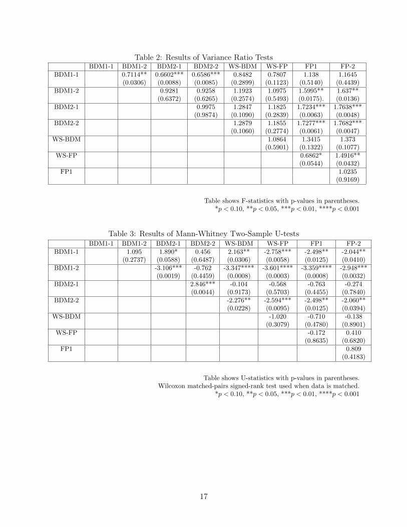
Table 2: Results of Variance Ratio TestsBDM1-1 BDM1-2 BDM2-1 BDM2-2 WS-BDM WS-FP FP1 FP-2

BDM1-1 0.7114** 0.6602*** 0.6586*** 0.8482 0.7807 1.138 1.1645(0.0306) (0.0088) (0.0085) (0.2899) (0.1123) (0.5140) (0.4439)

BDM1-2 0.9281 0.9258 1.1923 1.0975 1.5995** 1.637**(0.6372) (0.6265) (0.2574) (0.5493) (0.0175). (0.0136)

BDM2-1 0.9975 1.2847 1.1825 1.7234*** 1.7638***(0.9874) (0.1090) (0.2839) (0.0063) (0.0048)

BDM2-2 1.2879 1.1855 1.7277*** 1.7682***(0.1060) (0.2774) (0.0061) (0.0047)

WS-BDM 1.0864 1.3415 1.373(0.5901) (0.1322) (0.1077)

WS-FP 0.6862* 1.4916**(0.0544) (0.0432)

FP1 1.0235(0.9169)

Table shows F-statistics with p-values in parentheses.*p < 0.10, **p < 0.05, ***p < 0.01, ****p < 0.001

Table 3: Results of Mann-Whitney Two-Sample U-testsBDM1-1 BDM1-2 BDM2-1 BDM2-2 WS-BDM WS-FP FP1 FP-2

BDM1-1 1.095 1.890* 0.456 2.163** -2.758*** -2.498** -2.044**(0.2737) (0.0588) (0.6487) (0.0306) (0.0058) (0.0125) (0.0410)

BDM1-2 -3.106*** -0.762 -3.347**** -3.601**** -3.359**** -2.948***(0.0019) (0.4459) (0.0008) (0.0003) (0.0008) (0.0032)

BDM2-1 2.846*** -0.104 -0.568 -0.763 -0.274(0.0044) (0.9173) (0.5703) (0.4455) (0.7840)

BDM2-2 -2.276** -2.594*** -2.498** -2.060**(0.0228) (0.0095) (0.0125) (0.0394)

WS-BDM -1.020 -0.710 -0.138(0.3079) (0.4780) (0.8901)

WS-FP -0.172 0.410(0.8635) (0.6820)

FP1 0.809(0.4183)

Table shows U-statistics with p-values in parentheses.Wilcoxon matched-pairs signed-rank test used when data is matched.

*p < 0.10, **p < 0.05, ***p < 0.01, ****p < 0.001

17

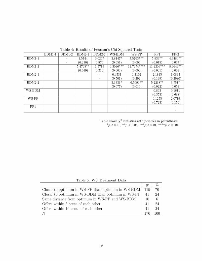
Table 4: Results of Pearson’s Chi-Squared TestsBDM1-1 BDM1-2 BDM2-1 BDM2-2 WS-BDM WS-FP FP1 FP-2

BDM1-1 - 1.5744 0.0267 3.8147* 7.5763*** 5.939** 4.3484**- (0.210) (0.870) (0.051) (0.006) (0.015) (0.037)

BDM1-2 5.4765** 1.5719 9.3036*** 14.7374**** 11.2209*** 8.9643**(0.019) (0.210) (0.002) (0.000) (0.001) (0.003)

BDM2-1 - 0.4531 1.1102 2.1845 1.0833- (0.501) (0.292) (0.139) (0.2980)

BDM2-2 3.1331* 6.5691** 5.2218** 3.751*(0.077) (0.010) (0.022) (0.053)

WS-BDM - 0.863 0.1611- (0.353) (0.688)

WS-FP 0.1255 2.0719(0.723) (0.150)

FP1 --

Table shows χ2 statistics with p-values in parentheses.*p < 0.10, **p < 0.05, ***p < 0.01, ****p < 0.001

Table 5: WS Treatment Data# %

Closer to optimum in WS-FP than optimum in WS-BDM 119 70Closer to optimum in WS-BDM than optimum in WS-FP 41 24Same distance from optimum in WS-FP and WS-BDM 10 6Offers within 5 cents of each other 41 24Offers within 10 cents of each other 41 24N 170 100

18

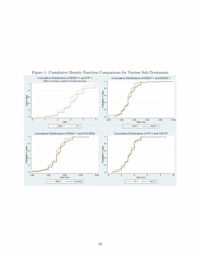
Figure 1: Cumulative Density Function Comparisons for Various Sub-Treatments

19

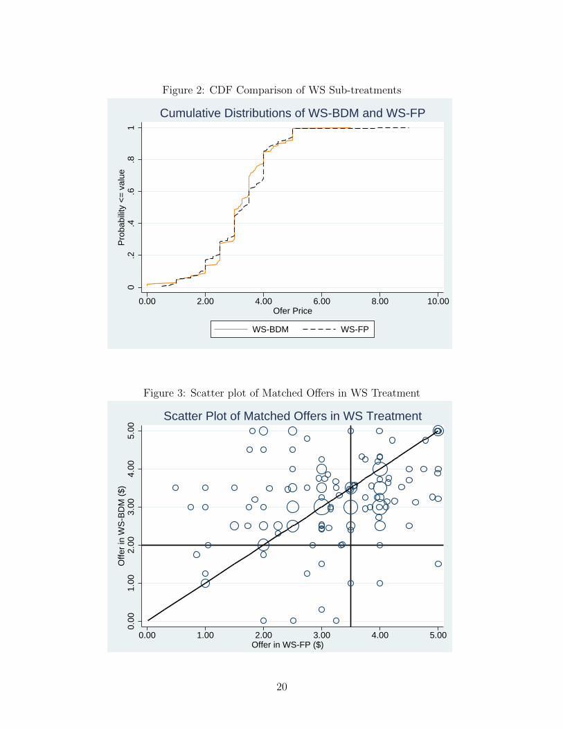
Figure 2: CDF Comparison of WS Sub-treatments

0.2

.4.6

.81

Pro

babi

lity

<=

val

ue

0.00 2.00 4.00 6.00 8.00 10.00Ofer Price

WS-BDM WS-FP

Cumulative Distributions of WS-BDM and WS-FP

Figure 3: Scatter plot of Matched Offers in WS Treatment

0.00

1.00

2.00

3.00

4.00

5.00

Offe

r in

WS

-BD

M (

$)

0.00 1.00 2.00 3.00 4.00 5.00

Scatter Plot of Matched Offers in WS Treatment

Offer in WS-FP ($)

20

7 Appendix

7.1 Replication of CP Results 3 and 5

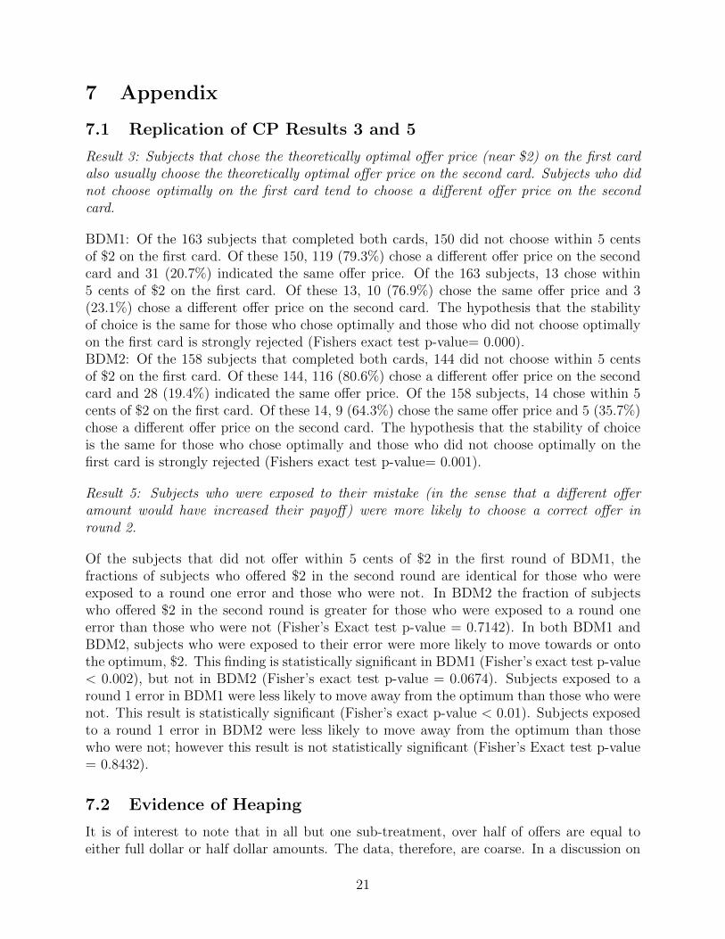
Result 3: Subjects that chose the theoretically optimal offer price (near $2) on the first cardalso usually choose the theoretically optimal offer price on the second card. Subjects who didnot choose optimally on the first card tend to choose a different offer price on the secondcard.

BDM1: Of the 163 subjects that completed both cards, 150 did not choose within 5 centsof $2 on the first card. Of these 150, 119 (79.3%) chose a different offer price on the secondcard and 31 (20.7%) indicated the same offer price. Of the 163 subjects, 13 chose within5 cents of $2 on the first card. Of these 13, 10 (76.9%) chose the same offer price and 3(23.1%) chose a different offer price on the second card. The hypothesis that the stabilityof choice is the same for those who chose optimally and those who did not choose optimallyon the first card is strongly rejected (Fishers exact test p-value= 0.000).BDM2: Of the 158 subjects that completed both cards, 144 did not choose within 5 centsof $2 on the first card. Of these 144, 116 (80.6%) chose a different offer price on the secondcard and 28 (19.4%) indicated the same offer price. Of the 158 subjects, 14 chose within 5cents of $2 on the first card. Of these 14, 9 (64.3%) chose the same offer price and 5 (35.7%)chose a different offer price on the second card. The hypothesis that the stability of choiceis the same for those who chose optimally and those who did not choose optimally on thefirst card is strongly rejected (Fishers exact test p-value= 0.001).

Result 5: Subjects who were exposed to their mistake (in the sense that a different offeramount would have increased their payoff) were more likely to choose a correct offer inround 2.

Of the subjects that did not offer within 5 cents of $2 in the first round of BDM1, thefractions of subjects who offered $2 in the second round are identical for those who wereexposed to a round one error and those who were not. In BDM2 the fraction of subjectswho offered $2 in the second round is greater for those who were exposed to a round oneerror than those who were not (Fisher’s Exact test p-value = 0.7142). In both BDM1 andBDM2, subjects who were exposed to their error were more likely to move towards or ontothe optimum, $2. This finding is statistically significant in BDM1 (Fisher’s exact test p-value< 0.002), but not in BDM2 (Fisher’s exact test p-value = 0.0674). Subjects exposed to around 1 error in BDM1 were less likely to move away from the optimum than those who werenot. This result is statistically significant (Fisher’s exact p-value < 0.01). Subjects exposedto a round 1 error in BDM2 were less likely to move away from the optimum than thosewho were not; however this result is not statistically significant (Fisher’s Exact test p-value= 0.8432).

7.2 Evidence of Heaping

It is of interest to note that in all but one sub-treatment, over half of offers are equal toeither full dollar or half dollar amounts. The data, therefore, are coarse. In a discussion on

21

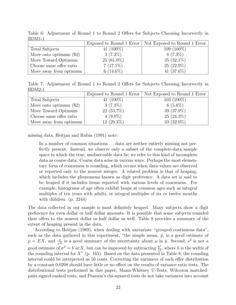
Table 6: Adjustment of Round 1 to Round 2 Offers for Subjects Choosing Incorrectly inBDM1-1

Exposed to Round 1 Error Not Exposed to Round 1 ErrorTotal Subjects 41 (100%) 109 (100%)Move onto optimum ($2) 3 (7.3%) 8 (7.3%)Move Toward Optimum 25 (61.0%) 35 (32.1%)Choose same offer ratio 7 (17.1%) 25 (22.9%)Move away from optimum 6 (14.6%) 41 (37.6%)

Table 7: Adjustment of Round 1 to Round 2 Offers for Subjects Choosing Incorrectly inBDM2-1

Exposed to Round 1 Error Not Exposed to Round 1 ErrorTotal Subjects 41 (100%) 103 (100%)Move onto optimum ($2) 3 (7.3%) 6 (5.8%)Move Toward Optimum 22 (53.7%) 39 (37.9%)Choose same offer ratio 4 (9.8%) 25 (24.3%)Move away from optimum 12 (29.3%) 33 (32.0%)

missing data, Heitjan and Rubin (1991) note:

In a number of common situations . . . data are neither entirely missing not per-fectly present. Instead, we observe only a subset of the complete-data samplespace in which the true, unobservable data lie; we refer to this kind of incompletedata as coarse data. Coarse data arise in various ways. Perhaps the most elemen-tary form of coarseness is rounding, which occurs when data values are observedor reported only to the nearest integer. A related problem is that of heaping,which includes the phenomena known as digit preference. A data set is said tobe heaped if it includes items reported with various levels of coarseness. Forexample, histograms of age often exhibit heaps at common ages such as integralmultiples of ten years with adults, or integral multiples of six or twelve monthswith children. (p. 2244)

The data collected in our sample is most definitely heaped. Many subjects show a digitpreference for even dollar or half dollar amounts. It is possible that some subjects roundedtheir offers to the nearest dollar or half dollar as well. Table 8 provides a summary of theextent of heaping present in the data.

According to Heitjan (1989), when dealing with univariate “grouped continuous data”,such as the data gathered in this experiment, “the simple mean, y, is a good estimate ofµ = EX, and s√

nis a good summary of the uncertainty about µ in y. Second, s2 is not a

good estimate of σ2 = V arX, but can be improved by subtracting h2

12, where h is the width of

the rounding interval for X” (p. 165). Based on the data presented in Table 8, the roundinginterval could be interpreted as 50 cents. Correcting the variances of each offer distributionby a constant 0.0208 should have little or no effect on the results of variance ratio tests. Thedistributional tests performed in this paper, Mann-Whitney U-Tests, Wilcoxon matched-pairs signed-ranked tests, and Pearson’s chi-squared tests do not take variances into account

22

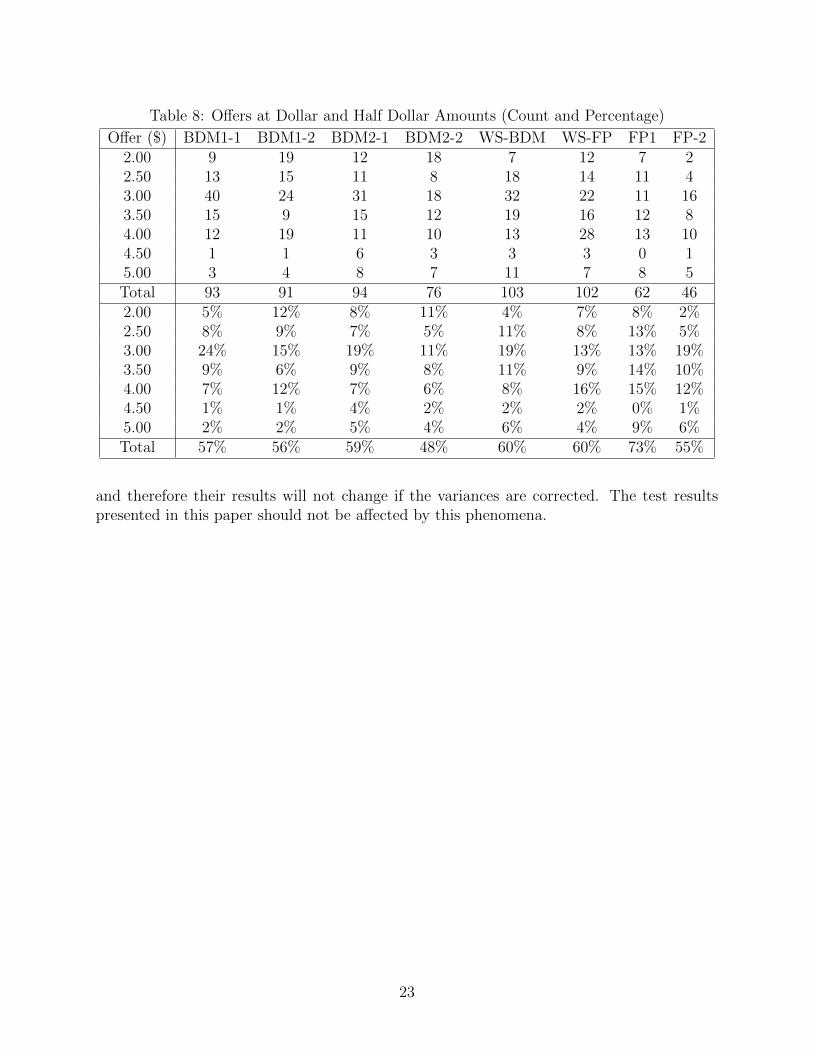
Table 8: Offers at Dollar and Half Dollar Amounts (Count and Percentage)

Offer ($) BDM1-1 BDM1-2 BDM2-1 BDM2-2 WS-BDM WS-FP FP1 FP-22.00 9 19 12 18 7 12 7 22.50 13 15 11 8 18 14 11 43.00 40 24 31 18 32 22 11 163.50 15 9 15 12 19 16 12 84.00 12 19 11 10 13 28 13 104.50 1 1 6 3 3 3 0 15.00 3 4 8 7 11 7 8 5Total 93 91 94 76 103 102 62 462.00 5% 12% 8% 11% 4% 7% 8% 2%2.50 8% 9% 7% 5% 11% 8% 13% 5%3.00 24% 15% 19% 11% 19% 13% 13% 19%3.50 9% 6% 9% 8% 11% 9% 14% 10%4.00 7% 12% 7% 6% 8% 16% 15% 12%4.50 1% 1% 4% 2% 2% 2% 0% 1%5.00 2% 2% 5% 4% 6% 4% 9% 6%Total 57% 56% 59% 48% 60% 60% 73% 55%

and therefore their results will not change if the variances are corrected. The test resultspresented in this paper should not be affected by this phenomena.

23

7.3 Information about Experiments

Decision card used for BDM1 treatment and WS-BDM sub-treatment:

Table 9: Payout Information by Treatment

BDM1 BDM2 WS FP TOTAverage $5.52 $4.43 $5.00 $4.50 $4.91Min $3.27 $2.00 $2.58 $2.00 $2.00Max $9.75 $7.66 $9.13 $7.00 $9.75N 164 159 171 85 579

24