How Not to Lie with Judicial Votes: Misconceptions ...
64
HoQuinn.FINAL.doc (Do Not Delete) 10/14/10 11:19 AM 813 How Not to Lie with Judicial Votes: Misconceptions, Measurement, and Models Daniel E. Ho† and Kevin M. Quinn†† INTRODUCTION The scholarship of judicial behavior might roughly be caricatured as follows. One view stemming from political science, with roots in legal realism, posits that judges are policymakers and that ideology, not legal doctrine, explains judicial decision making. 1 The contrary view from much of the legal Copyright © 2010 California Law Review, Inc. California Law Review, Inc. (CLR) is a California nonprofit corporation. CLR and the authors are solely responsible for the content of their publications. † Professor of Law & Robert E. Paradise Faculty Fellow for Excellence in Teaching and Research, Stanford Law School, 559 Nathan Abbott Way, Stanford, CA 94305; Tel: 650-723- 9560; Fax: 650-725-0253; Email: [email protected]; URL: http://dho.stanford.edu. †† Professor of Law, University of California, Berkeley, School of Law, 490 Simon Hall, Berkeley, CA 94720; Tel: 510-642-2485; Fax: 510-642-3767; Email: [email protected]; URL: http://law.berkeley.edu/kevinmquinn.htm. We thank Melissa Deas, Tony Fader, Ellen Medlin, Erica Ross, and Neal Ubriani for outstanding research assistance; Josh Fischman, Jim Gibson, Rick Lempert, Andrew Martin, Jeff Strnad, Chris Zorn, and the participants at the Conference on Building Theory Through Empirical Legal Studies at the University of California, Berkeley, for helpful comments and conversations; and Robert Anderson and Lee Epstein for generously sharing data. This work was supported by the National Science Foundation (SES 07-51834). 1. See Saul Brenner & Harold J. Spaeth, Stare Indecisis: The Alteration of Precedent on the Supreme Court, 1946-1992 109 (1995); David W. Rohde & Harold J. Spaeth, Supreme Court Decision Making 72 (1976) (arguing that judges “base their decisions solely upon personal policy preferences”); Glendon Schubert, The Judicial Mind: The Attitudes and Ideologies of Supreme Court Justices, 1946-1963 10 (1965) (“I shall attempt to provide a substantive interpretation of the major trends in the Court’s policy-making . . . on the basis of measurements of aggregate data relating primarily to the manifest voting behavior and inferred political attitudes of the justices.”); Jeffrey A. Segal & Harold J. Spaeth, The Supreme Court and the Attitudinal Model Revisited 86 (2002) (“Simply put, Rehnquist votes the way he does because he is extremely conservative; Marshall voted the way he did because he was extremely liberal.”); Jeffrey A. Segal & Harold J. Spaeth, The Supreme Court and the Attitudinal Model 65 (1993) (“[T]he Supreme Court decides disputes in light
Transcript of How Not to Lie with Judicial Votes: Misconceptions ...

HoQuinn.FINAL.doc (Do Not Delete) 10/14/10 11:19 AM
813
How Not to Lie with Judicial Votes: Misconceptions, Measurement, and
Models
Daniel E. Ho† and Kevin M. Quinn††
INTRODUCTION The scholarship of judicial behavior might roughly be caricatured as
follows. One view stemming from political science, with roots in legal realism, posits that judges are policymakers and that ideology, not legal doctrine, explains judicial decision making.1 The contrary view from much of the legal
Copyright © 2010 California Law Review, Inc. California Law Review, Inc. (CLR) is a
California nonprofit corporation. CLR and the authors are solely responsible for the content of their publications.
† Professor of Law & Robert E. Paradise Faculty Fellow for Excellence in Teaching and Research, Stanford Law School, 559 Nathan Abbott Way, Stanford, CA 94305; Tel: 650-723-9560; Fax: 650-725-0253; Email: [email protected]; URL: http://dho.stanford.edu.
†† Professor of Law, University of California, Berkeley, School of Law, 490 Simon Hall, Berkeley, CA 94720; Tel: 510-642-2485; Fax: 510-642-3767; Email: [email protected]; URL: http://law.berkeley.edu/kevinmquinn.htm.
We thank Melissa Deas, Tony Fader, Ellen Medlin, Erica Ross, and Neal Ubriani for outstanding research assistance; Josh Fischman, Jim Gibson, Rick Lempert, Andrew Martin, Jeff Strnad, Chris Zorn, and the participants at the Conference on Building Theory Through Empirical Legal Studies at the University of California, Berkeley, for helpful comments and conversations; and Robert Anderson and Lee Epstein for generously sharing data. This work was supported by the National Science Foundation (SES 07-51834).
1. See Saul Brenner & Harold J. Spaeth, Stare Indecisis: The Alteration of Precedent on the Supreme Court, 1946-1992 109 (1995); David W. Rohde & Harold J. Spaeth, Supreme Court Decision Making 72 (1976) (arguing that judges “base their decisions solely upon personal policy preferences”); Glendon Schubert, The Judicial Mind: The Attitudes and Ideologies of Supreme Court Justices, 1946-1963 10 (1965) (“I shall attempt to provide a substantive interpretation of the major trends in the Court’s policy-making . . . on the basis of measurements of aggregate data relating primarily to the manifest voting behavior and inferred political attitudes of the justices.”); Jeffrey A. Segal & Harold J. Spaeth, The Supreme Court and the Attitudinal Model Revisited 86 (2002) (“Simply put, Rehnquist votes the way he does because he is extremely conservative; Marshall voted the way he did because he was extremely liberal.”); Jeffrey A. Segal & Harold J. Spaeth, The Supreme Court and the Attitudinal Model 65 (1993) (“[T]he Supreme Court decides disputes in light

HoQuinn.FINAL.doc (Do Not Delete) 10/14/10 11:19 AM
814 CALIFORNIA LAW REVIEW [Vol. 98:813
academy, practicing bar, and bench is that such simplifications at best characterize a limited set of close cases, and at worst are wrongheaded and pernicious to the rule of law.2 While the debate dons different robes—“law vs. policy,” “legalism vs. attitudinalism,” or “formalism vs. skepticism”—perhaps its most salient attribute is that it is overblown, poses a false dichotomy, and has few truly devout adherents on either side.3 of the facts of the case vis-à-vis the ideological attitudes and values of the justices.”); Robert A. Dahl, Decision-Making in a Democracy: The Supreme Court as a National Policy-Maker, 6 J. Pub. L. 279, 280 (1957) (referring to the “fiction” that the Court is not a political body); Micheal W. Giles et al., Picking Federal Judges: A Note on Policy and Partisan Selection Agendas, 54 Pol. Res. Q. 623 (2001); Jeffrey A. Segal & Albert D. Cover, Ideological Values and the Votes of U.S. Supreme Court Justices, 83 Amer. Pol. Sci. Rev. 557, 557 (1989) (describing the dependence of votes on policy preferences as “[t]he fundamental assumption about the behavior of Supreme Court justices”).
2. See Wayne Batchis, Constitutional Nihilism: Political Science and the Deconstruction of the Judiciary, 6 Rutgers J.L. & Pub. Pol’y 1, 19 (2008) (“The objectivity that marks judicial professionalism is crafted through years of study and practice.”); Harry T. Edwards, Collegiality and Decision Making on the D.C. Circuit, 84 Va. L. Rev. 1335, 1335 (1998) (writing “to refute the heedless observations of academic scholars who misconstrue and misunderstand the work of the judges” and noting “that, in most cases, judicial decision making is a principled enterprise that is greatly facilitated by collegiality among judges”); Harry T. Edwards, Public Misperceptions Concerning the “Politics” of Judging: Dispelling Some Myths About the D.C. Circuit, 56 U. Colo. L. Rev. 619, 620 (1985) (“[I]t is the law—and not the personal politics of individual judges—that controls judicial decision-making . . . .”); John C.P. Goldberg, What Nobody Knows, 104 Mich. L. Rev. 1461, 1482–84 (2006) (“Suppose we see a justice who was appointed by a Republican president voting to grant states broad immunity from suit in federal court. . . . [W]hy is this an attitude, rather than a substantive view about the proper place of the state and federal governments in our constitutional scheme of government?”); Mark Tushnet, Post-Realist Legal Scholarship, 1980 Wisc. L. Rev. 1383, 1397 (1980) (referring to attitudinalists as “vote-counters” who “suffer[] from an unbearable simple-mindedness”); Patricia M. Wald, A Response to Tiller and Cross, 99 Colum. L. Rev. 235, 235 (1999) (describing judging as “a complex, case-specific, and subtle task that defies single-factor analysis”).
3. See Frank B. Cross, Political Science and the New Legal Realism: A Case of Unfortunate Interdisciplinary Ignorance, 92 Nw. U. L. Rev. 251, 310 (1997) (“Both attitudinal and legal perspectives are essential to providing an accurate description of judicial decisionmaking.”); Barry Friedman, Taking Law Seriously, 4 Persp. on Pol. 261, 264 (2006) (“[A]ttitudes and law both play a role . . . . [T]he question is not so much whether law plays a role, as what role it plays.”); Howard Gillman, Martin Shapiro and the Movement from “Old” to “New” Institutionalist Studies in Public Law Scholarship, 7 Ann. Rev. Pol. Sci. 363 (2004); Martin Shapiro, Political Jurisprudence, 52 Ky. L.J. 294, 330 (1964) (“[N]o political jurist has ever claimed that the new methods were either totally independent or sufficient means of examining the work of courts.”); C. Herman Pritchett, The Development of Judicial Research, in Frontiers of Judicial Research 27, 42 (Joel B. Grossman & Joseph Tanenhaus eds., 1969) (“[P]olitical scientists who have done so much to put the ‘political’ in ‘political jurisprudence’ need to emphasize that it is still ‘jurisprudence.’ It is judging in a political context, but it is still judging.”); Matthew C. Stephenson, Legal Realism for Economists, 23 J. Econ. Persp. 191, 197 (2009) (suggesting movement “beyond a crude ‘law vs. ideology’ debate toward a more nuanced understanding of the relationships among law, facts, judicial preferences, and case outcomes”); David R. Stras, The Incentives Approach to Judicial Retirement, 90 Minn. L. Rev. 1417, 1430 (2006) (“I believe that policy plays a role in the decisions of the Supreme Court, but it combines with a number of other considerations, including legal constraints . . . to shape the decision-making process.”); Stephen B. Burbank, On the Study of Judicial Behaviors: Of Law, Politics, Science, and Humility 1 (U. Pa. Law Sch. Pub. Law & Legal Theory Research Paper Series,
HoQuinn.FINAL.doc (Do Not Delete) 10/14/10 11:19 AM
2010] HOW NOT TO LIE WITH JUDICIAL VOTES 815
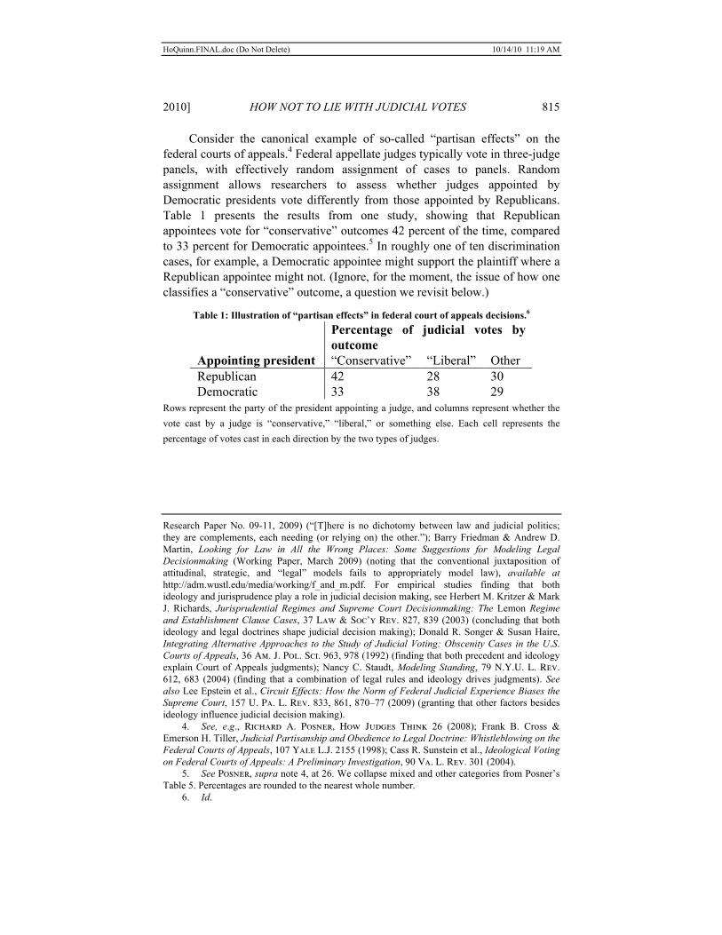
Consider the canonical example of so-called “partisan effects” on the federal courts of appeals.4 Federal appellate judges typically vote in three-judge panels, with effectively random assignment of cases to panels. Random assignment allows researchers to assess whether judges appointed by Democratic presidents vote differently from those appointed by Republicans. Table 1 presents the results from one study, showing that Republican appointees vote for “conservative” outcomes 42 percent of the time, compared to 33 percent for Democratic appointees.5 In roughly one of ten discrimination cases, for example, a Democratic appointee might support the plaintiff where a Republican appointee might not. (Ignore, for the moment, the issue of how one classifies a “conservative” outcome, a question we revisit below.)
Table 1: Illustration of “partisan effects” in federal court of appeals decisions.6 Percentage of judicial votes by
outcome Appointing president “Conservative” “Liberal” Other Republican 42 28 30 Democratic 33 38 29
Rows represent the party of the president appointing a judge, and columns represent whether the vote cast by a judge is “conservative,” “liberal,” or something else. Each cell represents the percentage of votes cast in each direction by the two types of judges.
Research Paper No. 09-11, 2009) (“[T]here is no dichotomy between law and judicial politics; they are complements, each needing (or relying on) the other.”); Barry Friedman & Andrew D. Martin, Looking for Law in All the Wrong Places: Some Suggestions for Modeling Legal Decisionmaking (Working Paper, March 2009) (noting that the conventional juxtaposition of attitudinal, strategic, and “legal” models fails to appropriately model law), available at http://adm.wustl.edu/media/working/f_and_m.pdf. For empirical studies finding that both ideology and jurisprudence play a role in judicial decision making, see Herbert M. Kritzer & Mark J. Richards, Jurisprudential Regimes and Supreme Court Decisionmaking: The Lemon Regime and Establishment Clause Cases, 37 Law & Soc’y Rev. 827, 839 (2003) (concluding that both ideology and legal doctrines shape judicial decision making); Donald R. Songer & Susan Haire, Integrating Alternative Approaches to the Study of Judicial Voting: Obscenity Cases in the U.S. Courts of Appeals, 36 Am. J. Pol. Sci. 963, 978 (1992) (finding that both precedent and ideology explain Court of Appeals judgments); Nancy C. Staudt, Modeling Standing, 79 N.Y.U. L. Rev. 612, 683 (2004) (finding that a combination of legal rules and ideology drives judgments). See also Lee Epstein et al., Circuit Effects: How the Norm of Federal Judicial Experience Biases the Supreme Court, 157 U. Pa. L. Rev. 833, 861, 870–77 (2009) (granting that other factors besides ideology influence judicial decision making).
4. See, e.g., Richard A. Posner, How Judges Think 26 (2008); Frank B. Cross & Emerson H. Tiller, Judicial Partisanship and Obedience to Legal Doctrine: Whistleblowing on the Federal Courts of Appeals, 107 Yale L.J. 2155 (1998); Cass R. Sunstein et al., Ideological Voting on Federal Courts of Appeals: A Preliminary Investigation, 90 Va. L. Rev. 301 (2004).
5. See Posner, supra note 4, at 26. We collapse mixed and other categories from Posner’s Table 5. Percentages are rounded to the nearest whole number.
6. Id.

HoQuinn.FINAL.doc (Do Not Delete) 10/14/10 11:19 AM
816 CALIFORNIA LAW REVIEW [Vol. 98:813
Such “partisan effects” demonstrate that Republican presidents nominate different types of appellate judges than Democratic presidents, but the correlation is far from perfect. Switching one-tenth of the votes might result in perfect agreement between Democratic and Republican appointees. The data stem exclusively from published cases, which may generate a false sense of partisan differences.7 Worse, such empirical results have been wildly misinterpreted as evidence for the primacy of politics over law and the conclusion that “judges are lawless.”8
While the correlation is suggestive of ideology, interpreting the results as evidence of “partisan effects” is misleading. The language of “effects” implies that the data reveal whether “ideology” or “law” caused outcomes, but the correlation cannot be interpreted causally.9 To crystallize the limitations of voting data, we can convert Table 1 to “partisan effects” in a survey of voters.
Table 2: Illustration of “partisan effects” in hypothetical voter survey. Percentage of vote by presidential
candidate Party of respondent Bush Gore Abstain Republican 42 28 30 Democratic 33 38 29
Cell numbers are identical to Table 1. Rows represent the party of a respondent, and columns represent whether a respondent voted for Bush, voted for Gore, or abstained.
Table 2 merely changes the labels on the judicial-voting data so that the units become individual respondents to a hypothetical survey. The rows now represent the partisan affiliation of the voter, instead of the appointing president’s party. Similarly, the columns now show the distribution of presidential votes cast, instead of case outcomes. Republicans in the hypothetical survey were nearly 10 percent more likely than Democrats to vote for Bush, and close to one-third of voters abstained. If the question forced upon Table 1 was whether policy or law causes judicial voting, the analogous question forced upon Table 2 might be whether partisanship or philosophy causes presidential voting.
7. See David S. Law, Strategic Judicial Lawmaking: Ideology, Publication, and Asylum
Law in the Ninth Circuit, 73 U. Cin. L. Rev. 817 (2005). 8. Edwards, Collegiality and Decision Making on the D.C. Circuit, supra note 2, at 1337. 9. The statistical literature on causal inference and law formalizes the conditions for causal
inference. See, e.g., John J. Donohue III & Daniel E. Ho, The Impact of Damage Caps on Malpractice Claims: Randomization Inference with Difference-in-Differences, 4 J. Empirical Legal Stud. 69 (2007); John J. Donohue & Justin Wolfers, Uses and Abuses of Empirical Evidence in the Death Penalty Debate, 58 Stan. L. Rev. 791 (2005); D. James Greiner, Causal Inference in Civil Rights Litigation, 122 Harv. L. Rev. 533 (2008); Daniel E. Ho et al., Matching as Nonparametric Preprocessing for Reducing Model Dependence in Parametric Causal Inference, 15 Pol. Anal. 199 (2007); Paul W. Holland, Statistics and Causal Inference, 81 J. Am. Stat. Ass’n 945 (1986); Jeff Strnad, Should Legal Empiricists Go Bayesian?, 9 Am. L. Econ. Rev. 195 (2007).

HoQuinn.FINAL.doc (Do Not Delete) 10/14/10 11:19 AM
2010] HOW NOT TO LIE WITH JUDICIAL VOTES 817
Both questions are ill-posed. To think of “partisan effects” causally, we must be able, at least in principle, to imagine an experiment that manipulates partisanship.10 While we might manipulate the language of a brief, the drafting of a statute, or the content of a legislative record, the manipulation of “ideology” stretches plausibility. How could we possibly manipulate a partisan belief system, let alone compare this effect with the impact of law or philosophy? Neither random sampling of survey respondents nor random assignment of cases to judges is a solution, as philosophy and jurisprudence are nowhere close to randomly assigned to respondents or judges. To the contrary, partisanship is horribly confounded: philosophical commitments might cause voters to register with different parties; and presidents may pick judges who individually exhibit principled jurisprudence that leads to different results, or is inapplicable, in subsets of close cases.
When partisan affiliation is a deliberate choice, such raw data cannot clearly answer the causal question of “law vs. politics.” To be sure, the correlation between partisan affiliation and outcomes is independently interesting, and studies of that correlation have provided significant insight into the federal judiciary.11 Presidential appointments matter.12 Some cases are close
10. See Holland, supra note 9. 11. See, e.g., Glendon A. Schubert, Quantitative Analysis of Judicial Behavior
(1959); Jilda M. Aliotta, Combining Judges’ Attributes and Case Characteristics: An Alternative Approach to Explaining Supreme Court Decisionmaking, 71 Judicature 277, 280 (1988) (finding that political party affiliation is a strong predictor of votes in equal protection cases); Sheldon Goldman, Voting Behavior on the United States Courts of Appeals, 1961–1964, 60 Amer. Pol. Sci. Rev. 374, 379 (1966) (finding correlations between “liberalism” and decisions in criminal, civil liberties, labor, private economic, combined injury, and activism cases); Stuart S. Nagel, Political Party Affiliation and Judges’ Decisions, 55 Amer. Pol. Sci. Rev. 843, 846 (1961) (observing that a judge’s partisan affiliation is strongly tied to his or her propensity to take the “liberal” or “conservative” position in certain types of cases); Donald R. Songer & Sue Davis, The Impact of Party and Region on Voting Decisions in the United States Courts of Appeals, 1955–1986, 43 W. Pol. Q. 317, 318 (1990) (describing “party differences in voting by judges on the courts of appeals” as “firmly established”); C. Neal Tate, Personal Attribute Models of the Voting Behavior of U.S. Supreme Court Justices: Liberalism in Civil Liberties and Economics Decisions, 1946–1978, 75 Amer. Pol. Sci. Rev. 355, 361–62 (1981) (finding that judicial voting in certain subject areas tracks partisan affiliation); S. Sidney Ulmer, The Political Party Variable in the Michigan Supreme Court, 11 J. Pub. L. 352, 360 (1962) (finding Democrats “more favorably inclined to workmen’s compensation claims than Republicans”). But see J. Woodford Howard, Jr., Courts of Appeals in the Federal Judicial System 186 (1981) (“The predictive power of political indicators was negligible and indirect.”); Orley Ashenfelter et al., Politics and the Judiciary: The Influence of Judicial Background on Case Outcomes, 24 J. Legal Stud. 257, 281 (1995) (“[W]e cannot find that Republican judges differ from Democratic judges in their treatment of civil rights cases.”).
12. See, e.g., Rohde & Spaeth, supra note 1; C.K. Rowland & Robert A. Carp, Politics and Judgment in Federal District Courts 24–57 (1996); Jon Gottschall, Carter’s Judicial Appointments: The Influence of Affirmative Action and Merit Selection on Voting on the U.S. Courts of Appeals, 67 Judicature 165, 173 (1983) (finding that Carter’s judicial appointees bring a liberal attitude to the bench which counterbalances the conservatism of the Nixon and Ford appointees); Jon Gottschall, Reagan’s Appointments to the U.S. Courts of Appeals: The Continuation of a Judicial Revolution, 70 Judicature 48, 49 (1986) (observing strong

HoQuinn.FINAL.doc (Do Not Delete) 10/14/10 11:19 AM
818 CALIFORNIA LAW REVIEW [Vol. 98:813
enough that the party of the appointing president predicts outcomes.13 And random assignment might uncover the impact of judicial assignment on litigants.14 But above all, such inferences about partisan effects are primarily descriptive or predictive, not causal.
So what questions do judicial votes allow us to address? Modern measurement methods provide one promising approach.15 Rapid advances in the statistical measurement of judicial behavior have provided concise, meaningful summaries of differences among judges based on their votes.
Yet while some laud these approaches as “ingenious,”16 “illuminating,”17 conservative tendencies in Reagan appointees); Edward V. Heck & Steven A. Shull, Policy Preferences of Justices and Presidents: The Case of Civil Rights, 4 Law & Pol’y Q. 327, 335 (1982) (finding a correlation between presidential preferences and the votes of the Justices they appointed); C. K. Rowland et al., Presidential Effects on Criminal Justice Policy in the Lower Federal Courts: The Reagan Judges, 22 Law & Soc’y Rev. 191, 195–96 (1988) (noting that Reagan appointees to district courts and courts of appeal are less supportive than Carter nominees of criminal defendants); Jeffrey A. Segal et al., Buyer Beware? Presidential Success through Supreme Court Appointments, 53 Pol. Res. Q. 557, 567 (2000) (finding that Supreme Court appointees initially support the political positions of their appointing president, though noting that some ideological drift may occur as time passes); Timothy B. Tomasi & Jess A. Velona, Note, All the President’s Men?: A Study of Ronald Reagan’s Appointments to the U.S. Courts of Appeals, 87 Colum. L. Rev. 766, 792 (1987) (finding that Republican-appointed judges are much more conservative than Democratic appointees, but that Reagan appointees are not significantly more conservative than Ford and Nixon judges).
13. See, e.g., Cross & Tiller, supra note 4, at 2168–71 (observing that the political party of the appointing president predicts votes in administrative law cases); Sunstein et al., supra note 4, at 305–06 (finding that the political party of the appointing president can predict judges’ votes in cases involving abortion, capital punishment, campaign finance, affirmative action, sex discrimination, sexual harassment, racial discrimination, disability discrimination, contract clause violation, and environmental regulation).
14. See, e.g., David S. Abrams & Albert H. Yoon, The Luck of the Draw: Using Random Case Assignment to Investigate Attorney Ability, 74 U. Chi. L. Rev. 1145 (2007); Radha Iyengar, An Analysis of the Performance of Federal Indigent Defense Counsel (Nat’l Bureau of Econ. Research, Working Paper No. 13187, 2007).
15. See, e.g., Lee Epstein, Kevin Quinn, Andrew D. Martin & Jeffrey A. Segal, On the Perils of Drawing Inferences About Supreme Court Justices from their First Few Years of Service, 91 Judicature 168 (2008); Lee Epstein, Daniel E. Ho, Gary King & Jeffrey A. Segal, The Supreme Court During Crisis: How War Affects Only Non-War Cases, 80 N.Y.U. L. Rev. 1 (2005); Joshua B. Fischman & David S. Law, What Is Judicial Ideology, and How Should We Measure It?, 29 Wash. U. J.L. & Pol’y 133 (2009); Daniel E. Ho & Kevin M. Quinn, Did a Switch in Time Save Nine?, 1 J. Legal Anal. (forthcoming 2010) (on file with the authors); Daniel E. Ho & Erica L. Ross, Did Liberal Justices Invent the Standing Doctrine? An Empirical Study of the Evolution of Standing, 1921–2006, 62 Stan. L. Rev. (forthcoming 2010) (on file with the authors); Daniel E. Ho & Kevin M. Quinn, Measuring Explicit Political Positions of the Media, 3 Q.J. Pol. Sci. 353 (2008); Daniel E. Ho & Kevin M. Quinn, Viewpoint Diversity and Media Consolidation: An Empirical Study, 61 Stan. L. Rev. 781 (2009). By “measurement methods,” we mean typically statistical approaches to inferring the value of a latent trait or attribute from the observable consequences of that latent trait or attribute.
16. Ward Farnsworth, The Use and Limits of Martin-Quinn Scores to Assess Supreme Court Justices, with Special Attention to the Problem of Ideological Drift, 101 Nw. U. L. Rev. 1891, 1891 (2007).
17. Theodore W. Ruger, Justice Harry Blackmun and the Phenomenon of Judicial Preference Change, 70 Mo. L. Rev. 1209, 1219 (2005).

HoQuinn.FINAL.doc (Do Not Delete) 10/14/10 11:19 AM
2010] HOW NOT TO LIE WITH JUDICIAL VOTES 819
and “highly sophisticated,”18 others call them “less than ideal [and] complicated,”19 “hard to follow,”20 and “blunt, if not outright misleading.”21 Confusion runs rampant: the scores that these methods yield are poorly understood, widely misinterpreted, and commonly misused.
To address this confusion, this Article synthesizes and unifies the understanding of statistical measures of judicial voting. It provides a guide for how to interpret such measures, clarifies misconceptions, and argues that the extant scores are merely a special case of a general approach to studying judicial behavior with (model-based) measurement.
In Part I, we describe the formal spatial theory often invoked to justify the statistical approach. While spatial theory has the nice feature of synthesizing theory and empirics, legal scholars may remain skeptical of its strong assumptions. Fortunately, measurement models can be illuminating even if the spatial theory is questionable. To illustrate this, Part II provides a nontechnical overview of the intuition behind measurement models that take merits votes as an input and return a summary score of Justice-specific behavior as an output.22 Such scores provide clear and intuitive descriptive summaries of differences in judicial voting.23
Confusion abounds, however, and in Part III we clarify prevailing misconceptions of such scores. We discuss how these scores relate to “ideology,” explain how such models grapple with the complexity and dimensionality of judicial decisionmaking, illustrate the problems of inter-temporal extrapolation and cardinal interpretation of the scores, and highlight other common abuses of such measures.
In Part IV, we demonstrate how modern measurement methods are useful precisely because they empower meaningful examination, data collection, and incorporation of doctrine and jurisprudence. We argue that existing uses are simply a special case of a much more general measurement approach that works synergistically with the qualitative study of case law. We demonstrate in Part V how such measurement approaches—when augmented with jurispruden-tially meaningful data—can advance our understanding of courts, with case
18. Fischman & Law, supra note 15, at 163. 19. James J. Brudney & Corey Ditslear, Canons of Construction and the Elusive Quest for
Neutral Reasoning, 58 Vand. L. Rev. 1, 20 n.83 (2005). 20. Farnsworth, supra note 16, at 1892. 21. Ruger, supra note 17, at 1219. 22. See, e.g., Joseph Bafumi et al., Practical Issues in Implementing and Understanding
Bayesian Ideal Point Estimation, 13 Pol. Anal. 171 (2005); Joshua Clinton et al., The Statistical Analysis of Roll Call Data, 98 Am. Pol. Sci. Rev. 355 (2004); Bernard Grofman & Timothy J. Brazill, Identifying the Median Justice on the Supreme Court Through Multidimensional Scaling: Analysis of “Natural Courts” 1953–1991, 112 Pub. Choice 55 (2002); Andrew D. Martin & Kevin M. Quinn, Dynamic Ideal Point Estimation via Markov Chain Monte Carlo for the U.S. Supreme Court, 1953–1999, 10 Pol. Analysis 134 (2002).
23. Parts I and II are for anyone interested in understanding these scores, but readers well-versed in the methods may choose to skip them.

HoQuinn.FINAL.doc (Do Not Delete) 10/14/10 11:19 AM
820 CALIFORNIA LAW REVIEW [Vol. 98:813
studies of the constitutional revolution of 1937, the dimensionality of the Supreme Court, the historical origins of the standing doctrine, statutory inter-pretation, and backlash against Supreme Court opinions. We conclude with thoughts on the chief virtues of model-based measurement and the study of law.
I INCREDIBLE VOTING THEORY
While the intellectual heritage of measurement models dates back to work in psychometrics,24 the canonical applications in political science deal with roll call votes in legislatures, particularly the U.S. Congress.25 In that context, the same models are known as ideal point models.
Researchers often invoke the so-called “spatial theory” of voting as the underpinning for the empirical ideal point model.26 While it is somewhat misleading to speak of the spatial theory—a voluminous literature describes numerous variants of such theories—the stylized version goes as follows. A roll call vote presents a binary choice between the status quo and an alternative in a typically unidimensional space (hence “spatial” theory).
Figure 1 represents this space, or latent dimension, on the x-axis. (Please note that all Figures appear at the end of this Article.) The hollow point marks the status quo, and the solid point marks the alternative. For example, the space could represent the possible minimum wages, with $7.25 at the status quo and a proposed alternative of $10.50. Decision makers are usually assumed to have preferences over this policy space, characterized by a utility function with a single peak at the decision maker’s preferred point. This utility function is plotted in as the curved line, with the y-axis showing the amount of utility. Utility decreases the farther away a policy is from the ideal point. The decision maker’s most preferred point in the space is her ideal point. For the minimum wage, for example, the decision maker might ideally prefer $9.50, but only the status quo of $7.25 or the proposal of $10.50 are available as voting choices. When confronted with a roll call, a legislator compares the utility of voting for the status quo to that of voting for the alternative, as the vertical arrow in Figure 1 indicates. Spatial theory posits that the legislator sincerely votes for
24. See Keith T. Poole, The Evolving Influence of Psychometrics in Political Science, in
The Oxford Handbook of Political Methodology 199 (Janet M. Box-Steffensmeier et al. eds., 2008) (tracing the intellectual lineage of modern ideal point models to work done in psychometrics in the early and mid-twentieth century).
25. See, e.g., Keith T. Poole & Howard Rosenthal, Congress: A Political-Economic History of Roll Call Voting (1997); Clinton et al., supra note 22; James J. Heckman & James M. Snyder, Jr., Linear Probability Models of the Demand for Attributes with an Empirical Application to Estimating the Preferences of Legislators, 28 RAND J. Econ S142 (1997).
26. Some refer to spatial theory as the spatial model. For expositional purposes, we use spatial theory to distinguish between theoretical models and empirical models.

HoQuinn.FINAL.doc (Do Not Delete) 10/14/10 11:19 AM
2010] HOW NOT TO LIE WITH JUDICIAL VOTES 821
the option with the highest relative utility—in other words, there is no vote trading or other strategic interaction that may affect these votes. Given the assumptions of the model, our hypothetical legislator would vote for the alternative.
This simple theory is quite useful within the context of legislative politics. It provides a concise description of legislative voting and many of its key assumptions—policy-motivated legislators, spatial preferences, binary choices—may be reasonable. Most powerfully, if one believes the assumptions underlying the theory, the observed votes of legislators allow for empirical inference of their ideal points.27 This structural interpretation of an ideal point model—justified by spatial theory—is common in political science and economics, and many researchers appear comfortable with such an interpretation in applications involving the U.S. Congress.28
Yet spatial theory appropriate for Congress may not apply directly to the judiciary. First, it is not obvious that a judge’s or Justice’s decision process is best thought of as a binary comparison of a clear status quo policy with a clear alternative policy.29 The decision space may not be continuous, and there may be no single status quo in a Supreme Court case addressing circuit splits. Second, judges and Justices may not be policymakers with well-behaved utility functions over the policy space; an appellate court judge may dissent even when the majority position leads to a policy outcome closer to her ideal point than the status quo. Third, judges and Justices may not vote in accordance with the model if they act strategically, such as by anticipating legislative or executive responses. Indeed, sophisticated theorists who posit a unidimensional policy space often do not subscribe to the sincere voting assumption themselves.30
27. On estimation details, see Poole & Rosenthal, supra note 25; Clinton et al., supra note 22; Heckman & Snyder, supra note 25. In practice, it is standard to assume some randomness so that votes become probabilistic.
28. Poole contrasts the primarily descriptive psychometric applications of ideal point models with the structural interpretation that many political scientists and economists favor. He writes:
The [methods] developed by psychologists were intended to help answer questions of importance to psychologists. . . . [R]esearchers could use [these] procedures to uncover underlying psychological dimensions or as a tool to formulate a convincing description of the data. . . . In contrast, the spatial theory of voting is a theory of behavior that states that if a set of assumptions holds, then voters should behave in a certain way and we should observe certain types of outcomes. It is a theory that makes predictions that can be tested.
Keith T. Poole, Spatial Models of Parliamentary Voting 9 (2005). 29. Throughout the paper, we will use the Supreme Court as an animating example, and
will hence often refer to the “Justices” even though the same methods can be applied to study appellate judges and regulators. See, e.g., Daniel E. Ho, Congressional Agency Control: The Impact of Statutory Partisan Requirements on Regulation (Feb. 12, 2007) (unpublished manuscript, on file with the authors), available at http://dho.stanford.edu/research/partisan.pdf.
30. See, e.g., John Ferejohn & Charles Shipan, Congressional Influence on Bureaucracy, 6 J.L. Econ & Org. 1, 6 (assuming “that all of the actors in the model prefer that their decisions not be overturned”); Calvin J. Mouw & Michael B. Mackuen, The Strategic Agenda in Legislative

HoQuinn.FINAL.doc (Do Not Delete) 10/14/10 11:19 AM
822 CALIFORNIA LAW REVIEW [Vol. 98:813
Using an ideal point model, however, does not require one to fully believe that judges act in accordance with spatial theory. Many researchers incorrectly assume that spatial theory is the only, or at least the primary, justification for the use of an empirical ideal point model, frequently leveling critiques at the theoretical, rather than statistical, assumptions.31 In the next Part, we sketch and explain measurement models that provide an alternative descriptive interpretation of ideal point models, rendering them useful even when the underlying spatial theory is implausible.
II CREDIBLE MEASUREMENT
Given that few legal academics subscribe to the strong assumptions of the spatial voting theory, should measurement models simply be ignored? No. “[A]ll models are wrong but some are useful.”32 Even if spatial theory is incredible, the statistical model may provide a credible, useful summary of differences in judicial voting.33 To understand this, we provide a conceptual, nontechnical overview of the statistical approach,34 and focus on issues of interpretation. As we will see, many criticisms of measurement models stem from misunderstandings—by critics, the original researcher, or both—about what estimates mean in concrete, substantive terms.
A. Measuring Intelligence Begin with a basic problem of measurement. Imagine you are an
instructor in a course with fifty students. You are responsible for writing a multiple-choice exam. What kinds of questions would you ask? Test questions
Politics, 86 Am. Pol. Sci. Rev. 87 (1992) (using a liberal-conservative dimension to study situations in which factors other than sincere preferences determines policy decisions); Matthew C. Stephenson, Legislative Allocation of Delegated Power: Uncertainty, Risk, and the Choice between Agencies and Courts, 119 Harv. L. Rev. 1035, 1037 (2006) (positing that legislators consider a tradeoff between interpretive consistency and risk diversification when delegating to courts or agencies).
31. See, e.g., Farnsworth, supra note 16, at 1893; Goldberg, supra note 2, at 1482–84. See also infra note 78.
32. G. E. P. Box, Robustness in the Strategy of Scientific Model Building, in Robustness in Statistics 201, 202 (Robert L. Launer & Graham N. Wilkinson eds., 1979).
33. Indeed, even if formal theory imposes assumptions that are wrong, the theoretical model may still be useful.
34. For more technical discussions, see Explanatory Item Response Models: A Generalized Linear and Nonlinear Approach (Paul De Boeck & Mark Wilson eds., 2004) (providing details on how covariates can be included in various ideal point models); Paul Gustafson, Measurement Error and Misclassification in Statistics and Epidemiology (2004) (detailing theory and methods for the general problem of making inferences about an unobserved variable from noisy indicators); Bafumi et al., supra note 22; Clinton et al., supra note 22; Simon Jackman, Multidimensional Analysis of Roll Call Data via Bayesian Simulation: Identification, Estimation, Inference and Model Checking, 9 Pol. Anal. 227 (2001) (providing an accessible introduction to ideal point models); Martin & Quinn, supra note 22.

HoQuinn.FINAL.doc (Do Not Delete) 10/14/10 11:19 AM
2010] HOW NOT TO LIE WITH JUDICIAL VOTES 823
must substantively relate to the material. However, easy questions that everyone answers correctly provide no meaningful information for distinguishing students. Similarly, hard questions that everyone answers incorrectly are not useful. Thus, one rule of thumb is to ask a question that discriminates well among students along the dimension of mastery of the course material.
How many questions would you need? One question would be insufficient. Students might have gotten the question right (or wrong) by chance. The question could have been poorly worded. Perhaps some students missed the day in class when the relevant material was covered. A simple distinction between those who got the right answer and those who did not might be a poor measure of what they learned. Only with more questions could we start to distinguish students on a fine-grained scale.
Measuring a concept as complex as “intelligence” through standardized testing exacerbates the measurement challenge. First, compared to a final exam for a single course covering discrete subject matter (e.g., geometry, physics, U.S. history), how do we administer, say, the SAT when there may be no agreed-upon notion of intelligence? Intelligence undoubtedly takes on many dimensions: verbal, quantitative, linguistic, emotional, spatial, and social, to name just a few.35 Considerable disagreement may exist over what intelligence even means. Yet rather than defining a priori the relevant notions of intelligence, standardized tests inductively define intelligence based on a set of test questions administered. We cannot directly observe intelligence, but each test question provides an indicator of an underlying “latent” (i.e., directly unobservable) dimension of intelligence.
Second, in a simple classroom setting it might be sufficient to calculate the proportion of correct answers and assign final grades based on these raw scores, but the SAT, as a matter of practicality, cannot be administered to all students at the same time. Some students take it in October and others in December. Lest students cheat, the questions cannot be the same for both of those tests. But what if December students are procrastinators and generally less intelligent than October students? Or what if the questions are simply harder on the December SAT? Scaling becomes a problem: in principle, a 1440 score in October should mean the same as a 1440 score in December. One solu-tion to this problem is to administer common questions to subsets of students in October and December.36 Such questions bridge the two tests. As long as there
35. See, e.g., Howard Gardner, Frames of Mind: The Theory of Multiple Intelligences (1983) (describing linguistic, logical-mathematic, spatial, bodily-kinesthetic, musical, interpersonal, and intrapersonal intelligences); L. L. Thurstone, Primary Mental Abilities (1938) (arguing that a test of only one ability cannot measure intelligence); Robert J. Sternberg, Myths, Countermyths, and Truths About Intelligence, 25 Educ. Res. 11, 11 (1996) (“The weight of the evidence at the present time is that intelligence is multidimensional.”).
36. Common item (nonequivalent group) design is of course only one method of scale equating. See Michael L. Kolen & Robert L. Brennan, Test Equating, Scaling, and

HoQuinn.FINAL.doc (Do Not Delete) 10/14/10 11:19 AM
824 CALIFORNIA LAW REVIEW [Vol. 98:813
are enough common questions, we can determine whether the October students differ meaningfully in underlying ability from the December students.37
How do we account for these common questions to derive the 2400 SAT scale? The clever solution to designing and analyzing tests is to model the probability of each test answer as a function of the latent dimension of interest. This allows the analyst to account for chance error in each test question, and to model the types of questions being administered.
Figure 2 illustrates the model-based adjustment for estimating intelligence from standardized test questions. The left panel (a) presents an “indiscriminate” question administered to a hypothetical set of fifty students. Answers from these fifty students are plotted as dots; the correct answers (at top) receive a score of one, and the incorrect answers (at bottom) receive a score of zero. The location of the point on the x-axis represents the latent dimension of intelligence for each student, which is posited to drive the majority of student responses. The y-axis represents the probability of a correct answer. This question is indiscriminate in that it distinguishes poorly between high- and low-ability students. The location of the dots on the latent dimension has virtually no relationship with the correctness of answers, and the probability curve has a slope close to zero. Designers of the SAT would want to discard this kind of test question.
In contrast, the question represented in the middle panel (b) discriminates quite well: only students with low values on the latent scale answered the question incorrectly, as shown by the cluster of grey dots in the lower-left corner. The “slope” of the probability curve is much greater than zero, meaning that high-ability students have a much greater chance of answering the question correctly.38 This is the kind of question test administrators seek to write, as it provides considerable information about the students.
The panels on the right demonstrate four other types of questions: panel (c) represents a hard, indiscriminate question (e.g., what is Avogadro’s number to twelve significant digits?); panel (d) represents an easy, indiscriminate question (e.g., who is the President of the United States?); panel (e) represents a poor question that intelligent students are actually more likely to get incorrect (e.g., is Newton’s first law of motion correct?); panel (f) represents an easy, but
Linking (2004) (explicating the theory underlying random group and nonequivalent group designs); Michael L. Kolen & Robert L. Brennan, Test Equating (Paul W. Holland & Donald B. Rubin eds., 1982) (detailing a number of model-based equating methods).
37. See, e.g., William H. Angoff, Summary and Derivation of Equating Methods Used at ETS, in Test Equating 55 (Paul W. Holland & Donald B. Rubin eds., 1982); Carl N. Morris, On the Foundations of Test Equating, in Test Equating 171 (Paul W. Holland & Donald B. Rubin eds. 1982); Nancy S. Petersen et al., Scaling, Norming, and Equating, in Educational Measurement 221 (Robert B. Linn ed., 3d ed. 1989).
38. We use the terms “slope” and “intercept” loosely here, given that the probability curve is nonlinear. The “slope” can be intuitively thought of as slope of the curve when the probability of a correct answer is 0.5.

HoQuinn.FINAL.doc (Do Not Delete) 10/14/10 11:19 AM
2010] HOW NOT TO LIE WITH JUDICIAL VOTES 825
only weakly discriminating question (e.g., apply the Pythagorean theorem). All of these scenarios can be captured by two question-specific parameters
that relate the test takers’ underlying abilities to the probability of correctly answering the question of interest. More formally, the probability of a correct response to question k by student j can be modeled as an increasing function of
. Let potentially range from negative infinity to positive infinity. When is large and positive, student j has a high probability of answering question k correctly; when is large in absolute value and negative student j has a low probability of answering question k correctly; and when it equals 0, student j has a 0.5 probability of answering question k correctly. Here is often referred to as the difficulty parameter for question k, is referred to as the discrimination parameter for question k, and is the ability of student j. These three “parameters” sufficiently characterize all of the panels of Figure 2.
Why this terminology and what does it mean intuitively? The ability is simply student j’s location along the latent dimension (i.e., intelligence). Higher values of mean that a student generally has a higher overall probability of answering a question correctly. For example, in panel (b) of Figure 2, students with higher abilities invariably answer the question correctly.
Now consider the difficulty parameter. When is much larger than zero, students will be unlikely to answer question k correctly regardless of the value of their ability; in other words, the question is difficult, as in panel (c) of Figure 2. When is much less than zero, students will be likely to answer question k correctly, regardless of the value of their ability; in other words, the question is easy, as in panel (d) of Figure 2. One can therefore think of as modeling the difficulty of the question by shifting the curves in Figure 2 up or down.
Now consider the discrimination parameter, which, roughly speaking, characterizes the slope of each curve. Note that the probability of a correct answer is determined by the product of ability and the discrimination parameter
. This means that when is large and positive, small increases in ability will lead to relatively large changes in the probability of correctly answering question k. In other words, the question discriminates well between high- and low-ability students, as in panel (b) of Figure 2. When is close to zero, there is essentially no relationship between ability and the probability of answering question k correctly. Put differently, the question does a poor job of discriminating, and the probability curve becomes a horizontal line as in panels (c), (d), and roughly (a) in Figure 2. When is less than zero, high-ability students overthink the question, and do worse than low-ability students, as in panel (e) of Figure 2.
As will become apparent, it is often useful to think of the cutpoint or cutline that separates students who have a better-than-50-percent chance of answering question k correctly from those that have a less-than-50-percent
HoQuinn.FINAL.doc (Do Not Delete) 10/14/10 11:19 AM
826 CALIFORNIA LAW REVIEW [Vol. 98:813
chance of a correct answer. Since we have assumed that this occurs at , the cutpoint is where equals .39
With this model for each test question, it becomes straightforward to adjust scores for types of questions. Intuitively, we downweight indiscriminate questions, and we give additional weight to questions that discriminate between high-ability and low-ability students. The key for educational testing is that the shape of the curve, particularly the slope, provides valuable information about how each test question is operating empirically. Applying such models to judicial votes allows one to infer the extent to which particular case decisions are consistent with a simple unidimensional ordering of the Justices. This turns out to be a key feature that empowers analysis of case law.
The main conceptual insights from educational testing are twofold. First, we are unlikely to be able to agree on an a priori definition of intelligence. Instead, we inductively design test questions that are indicators of intelligence. One might still challenge whether these questions capture the full scope of intelligence, but we might generally agree that they inductively measure some notion of intelligence. As we argue below, baseline estimates can thereby serve as a starting point for productive inquiry into deviations from the latent dimension. Second, the model-based adjustment for each test question allows us to account for measurement uncertainty, namely that answers to each question have some chance component unrelated to the target concept of intelligence. And the slope represents a rough measure of how much weight each question is given in the final score.
B. Measuring Judicial Views Why is the SAT relevant for the statistical analysis of judicial votes? It
turns out that the same class of models is adaptable to the study of judicial voting. In each case, we are interested in summarizing a complex latent attribute (scholarly aptitude or jurisprudential views) using information from a set of binary choices—correct versus incorrect answer on a test item or affirm versus reverse in a case. Switch questions with cases, students with Justices, and intelligence with jurisprudence, and the model proves almost directly applicable.
This measurement approach has one chief attractive feature. Jurisprudence, merits views, or “ideal points” of the Justices on the Supreme Court, just like the intelligence of students, are notoriously complex and difficult to summarize. Yet we can think of the votes in each case as an indicator of underlying differences among the Justices in a single latent dimension. Just as the analysis of the SAT reduces the highly complex and
39. In the context of the simple spatial model of Part I, and are functions of the status
quo and alternative policy positions while is the most preferred policy position of Justice j (his or her ideal point).

HoQuinn.FINAL.doc (Do Not Delete) 10/14/10 11:19 AM
2010] HOW NOT TO LIE WITH JUDICIAL VOTES 827
undoubtedly multidimensional concept of intelligence to a single dimension that is a weighted average across questions, the analysis of judicial voting reduces jurisprudence to a single dimension that is a weighted average across cases. And just as the SAT has no natural interpretation of scores in the 600 to 2400 range, the cardinal values in the latent dimension have no inherent interpretation; instead, it is a relative scale that best distinguishes between subjects’ observed answers or votes.
1. Modeling Votes How do we adapt the SAT model to judicial votes? Figure 3 applies the same type of probability model depicted in Figure 2 to three sample cases. (The curves of the first two panels are in fact identical for both figures.) One complication of the judicial voting model compared to the SAT scaling is that there is no “correct” vote. More specifically, the votes we use are not directionally coded in a “liberal” or “conservative” (or any other meaningful) direction; instead, each vote is coded as in the majority or minority with respect to the judgment in the case. While we could use directionally coded votes, nondirectional votes have a considerable advantage of circumventing the difficulty of manually classifying votes. Rather than engage in such manual classification, we defined the scale by setting two Justices to be on opposite sides of the origin: here, Justice Thomas is set to be “positive” and Justice Stevens is set to be “negative.” All other Justices are then ultimately estimated in the model relative to the anchors. Since the scale is entirely relative, one could equivalently constrain Justice Stevens to be greater than Justice Thomas, use two other Justices, or set any two Justices at points other than the extremes while estimating the other Justices.40 The constraints simply fix the direction of the scale.41 And because it is relatively uncontroversial to think that Justices Thomas and Stevens characterize different directions of the spectrum, interpreting the results relative to this assumption is by and large reasonable.
The y-axis in Figure 3 represents the probability of a vote in line with the majority and the x-axis represents the latent dimension with Justices Thomas and Stevens set on opposite sides. The left panel displays the votes for Blakely v. Washington,42 which involved the question of whether a state trial court’s sentencing of a defendant beyond the maximum statutory range on the basis of facts not found by a jury or admitted by the defendant violates the Sixth
40. Some complications arise when we pick two Justices who are quite similar in their voting patterns (e.g., Kennedy and O’Connor), and it is usually best to use substantive information to anchor the scales. See Bafumi et al., supra note 22.
41. See Bafumi et al., supra note 22; Clinton et al., supra note 22; John Londregan, Estimating Legislators’ Preferred Points, 8 Pol. Anal. 35 (2000). Technically, we also need to set the magnitude of the scale, which in our approach is achieved by the prior distribution of the ideal points and cutlines. Of course, there is not much substantive meaning behind cardinal values (e.g., the scaling of the SAT from 600–2400 versus 40–160). See Part III.B below.
42. 542 U.S. 296 (2004).

HoQuinn.FINAL.doc (Do Not Delete) 10/14/10 11:19 AM
828 CALIFORNIA LAW REVIEW [Vol. 98:813
Amendment. Justice Scalia, in an opinion joined by Justices Stevens, Souter, Thomas, and Ginsburg, found that the sentence violated the Sixth Amendment. Justices O’Connor, Breyer, Kennedy, and Rehnquist dissented in a complex series of opinions. Because the coalitions are atypical, the slope for Blakely is effectively zero, as illustrated by the 95 percent uncertainty bands. We learn little from this case about the Justices’ locations in the latent dimension.
Contrast Blakely with the decisions in Gratz v. Bollinger43 and Grutter v. Bollinger,44 the set of affirmative action cases involving the constitutionality of the undergraduate and law school admissions policies at the University of Michigan. In Gratz, the six-Justice majority found the undergraduate-level practice of awarding twenty extra admissions points to minority applicants violated equal protection because it was not narrowly tailored to achieve the university’s diversity objective. In contrast, in Grutter, the five-Justice majority upheld the law school’s consideration of race as a positive factor in individualized assessments of student applications. Justices Breyer and O’Connor provided the key votes distinguishing the outcomes in Gratz and Grutter. For both cases, the slope is sharply different from zero, showing that the latent dimension is highly predictive of votes in these cases. For Gratz, the slope is positive, meaning that Justices closer to Justice Thomas were more likely to vote for the majority, whereas for Grutter, the slope is negative, meaning that Justices closer to Justice Stevens were more likely to vote for the majority. The sign of the slope thereby differentiates the directionality of a case. The absolute magnitude of the slope represents how much weight to accord a case by indicating how informative it is about the position of the Justices in the latent dimension. Just like a poor test question, Blakely contributes very little information, while Gratz and Grutter contribute quite a lot. Moreover, the model is probabilistic. The probability of Justice Breyer joining the majority in Gratz, as he did, is low (roughly 0.29), but the measurement model clearly allows for divergences from systematic patterns for idiosyncratic reasons.
2. Learning From Votes Now that we understand the vote model at the case-level, how can we
incorporate votes to draw inferences about Justice locations along the latent dimension? The measurement approach engages in a form of “Bayesian learning” about the locations of the Justices, jointly estimating the case parameters and the latent position. Bayesian learning is the process of incorporating information to form a belief about an uncertain quantity.45 For
43. 539 U.S. 244 (2003). 44. 539 U.S. 306 (2003). 45. See generally Andrew Gelman et al., Bayesian Data Analysis (2d ed. 2003);
Michael O. Finkelstein & William B. Fairley, A Bayesian Approach to Identification Evidence, 83 Harv. L. Rev. 489 (1970); Strnad, supra note 9.

HoQuinn.FINAL.doc (Do Not Delete) 10/14/10 11:19 AM
2010] HOW NOT TO LIE WITH JUDICIAL VOTES 829
example, suppose that students are randomly entering into a classroom and that their median height is 5’5”. The probability that an entering student is taller than 5’5” is 50 percent, since the median height separates exactly half of the students as above or below it. But what if we are told that the student is male? The probability estimate should change; since men are on average taller than women, the probability should be greater than 50 percent. This process of updating a probability to incorporate new information—that the student is male—is the gist of Bayesian learning. Figure 4 illustrates the Bayesian learning process that occurs as each case of the 2000 Supreme Court Term is issued, allowing beliefs about the location of the Justices along the latent dimension to evolve. The top panel presents votes in each nonunanimous case of the Term. The columns represent cases sorted in chronological order from left to right, and each row represents a Justice. The shading in each cell represents how a Justice voted in the case: dark grey for minority, light grey for majority, and white if the Justice did not participate in a case. The first observed case, City of Indianapolis v. Edmond46 in the third column, for example, resulted in a 6–3 vote, with Justices Thomas, Scalia, and Rehnquist in the minority. The bottom panel presents our “beliefs” about the ranking of the Justices, from one to nine, in the latent dimension after observing the votes in each case. The first column is uniformly grey to depict a “prior” belief of identical locations of the Justices; hence there are no votes associated with that column in the top panel. The second column imposes the directional constraint that Justice Thomas ranks above Justice Stevens in the latent dimension. With the poles of the model thus set, we can draw inferences about the other Justices relative to Justices Stevens and Thomas after observing the votes in each case. Consider the point at which the first case is decided: as Edmond presents a 6–3 split, our new belief reflects exactly that ordering, ranking Justices Stevens, Ginsburg, Breyer, Souter, O’Connor, and Kennedy below Justices Rehnquist, Scalia, and Thomas in the latent dimension.
As each additional case is decided, our belief about the relative ranks becomes more precise. For example, after Bush v. Gore47 (the second case), there are roughly three blocs: (a) Justices Stevens, Ginsburg, Breyer, and Souter; (b) Justices O’Connor and Kennedy; and (c) Justices Rehnquist, Scalia, and Thomas. Justice Breyer’s solo dissent in Gitlitz v. Commissioner of the IRS48 (the fourth case) briefly leads us to infer that he is the lowest-ranked Justice in the latent dimension. (Note that the directional constraint does not require that Justices Stevens or Thomas occupy the lowest or highest ranks.) Yet that belief changes quickly with Justice Stevens’s propensity to dissent alone in cases like Seling v. Young49 and Illinois v. McArthur.50 Justices
46. 531 U.S. 32 (2000). 47. 531 U.S. 98 (2000). 48. 531 U.S. 206 (2001). 49. 531 U.S. 250 (2001).

HoQuinn.FINAL.doc (Do Not Delete) 10/14/10 11:19 AM
830 CALIFORNIA LAW REVIEW [Vol. 98:813
Stevens and Breyer voted together in enough cases like Egelhoff v. Egelhoff51 and Atwater v. City of Lago Vista52 that they become roughly tied for a short period some twenty nonunanimous cases into the Term. After observing all voting blocs for the Term (45 nonunanimous cases with 403 total votes cast), we arrive at the ranks in the rightmost column, with Justice Stevens as the lowest-ranked Justice, followed by Justices Ginsburg and Breyer, then Justice Souter, then Justices O’Connor and Kennedy, then Justice Rehnquist, and finally Justices Thomas and Scalia.
The bars behind the names of the cases also depict the weight the model assigns to each decision (i.e., the absolute value of the slope of the probability component for each case); this provides a relative sense of which cases contribute significantly to learning about the locations of the Justices. The latent dimension does a poor job, for example, of classifying votes in Kyllo v. United States,53 which presented the question of whether the use of a thermal imaging device to monitor a home constitutes a “search” under the Fourth Amendment. The voting split was atypical, with Justices Scalia, Souter, Thomas, Ginsburg, and Breyer finding that it constitutes a search. Just like test questions that discriminate poorly, Kyllo adds little to our belief about the relative positions of the Justices.
The lower right-hand panel summarizes the ideal points’ evolution over the course of the Term. For each Justice, the best guess of the ideal point is plotted over time, with grey lines representing the other Justices. Justices Thomas and Scalia continuously move upwards, while Justice Stevens continuously moves downwards, relative to the other Justices.
While Figure 4 illustrates the process of Bayesian learning, the knowledge gained is limited to the 45 nonunanimous cases from the 2000 Term. Even if we were simply trying to observe differences among nine students, 45 test questions may not allow us to learn very much. Contrast the SAT, which includes some 170 questions. The rightmost column of Figure 4 reflects the resulting uncertainty, with the data by and large insufficient to allow us to distinguish Justices Thomas and Scalia, Justices Kennedy and O’Connor, and Justices Breyer and Ginsburg.
Figure 5 therefore includes results from applying the model to all nonunanimous cases (nearly 500) of the Rehnquist Court (1994–2004).54 The left panel presents the locations in the latent dimension by short vertical marks, with the horizontal 95 percent bands reflecting uncertainty about the position. The bottom bar plots estimated cutlines for each case. (Recall that cutlines are
50. 531 U.S. 326 (2001). 51. 532 U.S. 141 (2001). 52. 532 U.S. 318 (2001). 53. 533 U.S. 27 (2001). 54. In fact, we applied the model to the Court from 1921–2006 (as displayed in Figure 6)
but present only the Rehnquist Court results in Figure 5.
HoQuinn.FINAL.doc (Do Not Delete) 10/14/10 11:19 AM
2010] HOW NOT TO LIE WITH JUDICIAL VOTES 831
the estimated position that splits the majority from the minority.) For example, the cluster of red lines represents roughly eighty cases with the conventional 5–4 split on the Rehnquist Court, with Justices Souter, Breyer, Ginsburg, and Stevens in the minority. The interpretation of the distance between ideal points is therefore entirely relative: all other things being equal, the distance between two Justices represents their difference in voting patterns; but this is also relative to the cutlines. For example, while the cardinal distance between Justice Thomas and Scalia is quite large, there are in fact relatively few cutlines separating them. While they are distinguishable, the number of cases in which they disagree is much smaller than the number of cases presenting the conventional 5–4 split. For this reason, we advocate always visualizing ideal points together with cutlines.
The right panel of Figure 5 plots the relative ranks of each of the Justices. The boxes represent the probability that a Justice occupies any one of the nine ranks, with shading proportional to probability. (In Figure 4, the shades instead represented expected ranks, but in Figure 5 they illustrate uncertainty over all ranks.) The precisely estimated ranks in Figure 5 incorporate all of the votes from the Rehnquist Court. Justice Stevens effectively has a 100 percent chance of occupying the leftmost position. The relative positions of Justices Breyer, Ginsburg, O’Connor, and Kennedy are less certain: Justice Breyer, for example, has probabilities of 0.135, 0.862, and 0.003 of occupying the second, third, and fourth positions, respectively. Overall, however, we have a fairly precise sense of where the Justices are located: for each Justice, the probability of occupying the rank in the order presented is greater than 0.85.
Figure 6 presents results for all of the Justices from 1921–2006.55 The x-axis represents the Terms of the Court; the y-axis represents the latent dimension, rotating the left-right dimension counterclockwise and transforming it for visibility, so that Justice Stevens is “below” Justice Thomas. Each red dot represents the estimated position for one Justice, with the horizontal lines representing the length of service. The blue dots represent the cutpoints for roughly 5,500 nonunanimous cases decided during this period. Justice Douglas, for example, is on the low edges of the space because of his great propensity to file solo dissents, depicted by the cluster of blue cutpoints separating him from Justices Black, Fortas, and Marshall. The model provides credible classifications of the Justices consistent with loose notions of “liberalism” that we clarify in Part III.A. For the Lochner Court sitting during the First New Deal (marked by the first vertical grey line), the “Four Horsemen” (Justices McReynolds, Butler, Sutherland, and Van Devanter) are estimated to be at the top of the space; the “Three Musketeers” (Justices Stone, Cardozo, and Brandeis) are at the bottom of the space; and the two swing Justices (Justice Roberts and Chief Justice Hughes) occupy the center.
55. We use backdated merits data compiled by Ho & Ross, supra note 15.

HoQuinn.FINAL.doc (Do Not Delete) 10/14/10 11:19 AM
832 CALIFORNIA LAW REVIEW [Vol. 98:813
The composition changed dramatically with President Franklin Delano Roosevelt’s (FDR’s) appointees. By 1941, FDR appointed seven new Justices, and the Court shifted substantially, as indicated by the second vertical grey line. Justices Frankfurter and Jackson, relatively “liberal” compared to the Lochner Court, anchor the more “conservative” end of the Roosevelt Court, with Justices Black and Douglas occupying the other end of the spectrum.
Figure 6 also illustrates what appears to be a gradual shift upwards over time, due in substantial part to the Nixon appointees.
3. Changes Over Time So far, we have assumed that the views of the Justices do not change over
time. This permits a rough characterization, but Figure 6 also hints at potential evolution over time. Consider Justice Blackmun’s position from 1970–94 relative to the cutlines. The cutlines gradually move above Justice Blackmun over this time period, suggesting that the caseload evolved so that Justice Blackmun came to side more with Justice Marshall over time, or that Justice Blackmun’s view itself may have evolved.
Examining such movement requires an additional modification to the SAT model. One approach might be to simply estimate ideal points separately for every Term that each Justice served, thereby assuming “independence” across every Term. But this sacrifices considerable precision in the estimates. Compare, for example, the relatively imprecise distinctions from only the 2000 Term votes—the lower right-hand ranks of Figure 4—with the precise ranks from the 1994–2004 Terms in the right panel of Figure 5. A small number of cases results in much more estimation uncertainty and variability, as if we tried to infer SAT scores from a single exam section alone. Moreover, it is substantively unreasonable: it makes little sense to assume that the views of the Justices arise independently for every Term.
The top left panel of Figure 7 shows, with hypothetical data, what happens when we estimate Term-specific ideal points for a Justice. The y-axis represents the latent dimension, the x-axis represents Terms, and the points and intervals present the now familiar ideal points with uncertainty bands. The intervals demonstrate a clear downward trend over time, but the estimates vary quite a bit across Terms: the intervals from 1972–73 are wider than those of 1970–71, and the hypothetical justice appears to be significantly more “conservative” in the 1982 Term.
The bottom right panel presents the other extreme: pooling all cases assuming constant positions as in Figure 6. The horizontal line represents the ideal point averaged across all Terms, with an uncertainty band that is much smaller than those of each of the separate Term estimates.
Instead of assuming constant or independent Term-by-Term estimates, one intermediate approach is to “smooth” the time trend. We do so by assuming estimates are closely related across Terms. One of the virtues of such
HoQuinn.FINAL.doc (Do Not Delete) 10/14/10 11:19 AM
2010] HOW NOT TO LIE WITH JUDICIAL VOTES 833
smoothing is that independence and complete pooling are merely special cases of this approach when the smoothness parameter (τ) approaches ∞ or 0, respectively. The researcher can specify or estimate the degree of smoothing. The top right panel shows the effects of weak pooling: the extreme estimates “shrink” slightly towards the global mean, but the amount of smoothing is minute. The bottom left panel engages in moderate smoothing: the 1982 Term shrinks back to the local mean, and the jagged patterns of the Term-by-Term estimates largely disappear. Nonetheless, the results reveal the evolution of the ideal points over time. Doing so for all the Justices allows for greater examination of dynamic trends, although the interpretation is nontrivial, as we discuss below.
C. Illustrations With this exposition, it becomes apparent that even when the relatively
strong assumptions of spatial theory do not hold, the estimates derived from ideal point models can still be quite useful. First, ideal point models permit rich, descriptive inferences about the relative propensities of various Justices to vote together. Second, ideal point models can provide a model-based method of selecting cases for further study, assessing violations of assumptions, and, more generally, incorporating more jurisprudentially meaningful information. We develop this last point more fully in Part III of this Article. Here, we briefly describe three applications effectively using ideal point models to make non-trivial descriptive inferences.
1. Who is the Median Justice? Supreme Court scholars have long been interested in identifying the
“center” of the Court, the “middle” of the Court, and the “swing Justice.”56 By summarizing judicial voting patterns as points on a line (or possibly in a higher-dimensional space, as we show in Part V.B below), ideal point estimates provide a natural means of locating the Court’s median Justice. Assuming that a single latent dimension summarizes voting, the Justice with four colleagues to the right and four colleagues to the left occupies the center position. While such a characterization is especially salient if one assumes that the basic spatial model of voting holds for the Court, a descriptive interpretation of the median Justice remains valid even without this assumption. Using data on merits votes from 1937–2002, Professors Andrew D. Martin, Kevin M. Quinn, and Lee Epstein calculated the probability that each Justice was the median member of
56. See, e.g., Symposium, Locating the Constitutional Center, 83 N.C. L. Rev. 1089
(2005). The articles in this symposium provide several perspectives on what the “center” of the Court might mean. Andrew D. Martin et al., The Median Justice on the United States Supreme Court, 83 N.C. L. Rev. 1275, 1276–77 & nn.1–6 (2005) provides numerous examples of how academics have used terms related to the “center” of the Court.

HoQuinn.FINAL.doc (Do Not Delete) 10/14/10 11:19 AM
834 CALIFORNIA LAW REVIEW [Vol. 98:813
the Court during each Term served.57 For some Terms the data successfully identifies the Court’s center. For instance, the posterior probability that Justice White was the Court’s median member in 1982 is effectively one.58 In other years, the median’s identity is less clear. During the 1991 Term, no Justice has more than a 35 percent chance of occupying the median position.59
Are these inferences valid if Justices are not acting in strict accordance with a spatial model of voting? As we point out below in Part III.D, the assumptions underlying standard ideal point models can have a large effect on the cardinal properties of estimates. Because there is no objective scale to the underlying latent space, different methods of normalization result in different ideal point estimates. Yet, while this relativity might seem troubling, calculating the median only requires ordinal information. Fortunately, ordinal properties of ideal point estimates are much less sensitive to prior assumptions than cardinal properties of the estimates.60 Consequently, identifying the Court’s median Justice does not require fully believing particular theoretical assumptions used to motivate an ideal point model.
More deeply, if the spatial model of voting does not hold, why is the median Justice’s identity a meaningful quantity of interest? As noted above, if the spatial model (and its assumption of a policy dimension) does not structure judicial behavior, then ideal point estimates are not necessarily representations of “ideology” or policy preferences. However, ideal point estimates will remain, by construction, reasonable summaries of judicial behavior. Knowing that one Justice is likely to occupy the median position implies that Justice is often the pivotal voter in 5–4 decisions.
2. Who Is the Most “Liberal” Justice? Order statistics other than the median are similarly well-behaved, even if
the spatial model of voting does not hold. We can use ideal point estimates to infer the location of the Justice who is farthest to the left on the latent dimension. In our example, where Justice Thomas is assumed to be on the positive side and Justice Stevens on the negative side of the latent dimension, the Justice with the leftmost ideal point can be considered the most “liberal.” We use “liberal” in quotation marks because we implicitly defined the concept through the relative placement of Justices Thomas and Stevens. Thus “liberal” actually means something more akin to “more Stevens-like and less Thomas-like” than liberal as a strict matter of political philosophy. We clarify this interpretation and the relationship of the latent dimension to jurisprudence and
57. Martin et al., supra note 56, at 1276–77, nn.1–6. 58. Id. at 1303. 59. Id. 60. Ordinal properties of a set of points depend only on the rank order of the points.
Cardinal properties depend on the actual numerical values of the ideal points (i.e., how far from the origin of zero they are).

HoQuinn.FINAL.doc (Do Not Delete) 10/14/10 11:19 AM
2010] HOW NOT TO LIE WITH JUDICIAL VOTES 835
ideology below in Part III.A.
3. How Did Justice Blackmun Evolve? Model-based measurement also allows for exploration of temporal
changes in a Justice’s voting patterns.61 Within a natural court, shifts in Term-by-Term ideal point ranks reveal changes; with the same nine members, well-defined ordinal comparisons alone prove sufficient. Making comparisons across stretches of time that feature membership change on the Court requires considerably more care.62 In such situations, intertemporal comparisons depend to a greater extent on untestable assumptions. We discuss this point more fully in Part III.C below.
To provide a concrete example, we focus on Justice Blackmun’s ideal point trajectory over his entire career as well as within a single natural court. Despite Justice Blackmun’s protestations,63 many scholars believe his jurisprudence changed markedly during his tenure on the bench.64
Figure 8 presents dynamic ideal point estimates for Justice Blackmun and his contemporaries on the Court.65 The left panel of Figure 8 displays ideal point estimates over Justice Blackmun’s entire career, showing evidence of leftward (or downward) drift—at least relative to his colleagues. The strongest evidence of this change is that Justice Blackmun’s ideal point series crosses over the ideal point series of several other Justices. Concretely, Justice Blackmun started off with voting patterns closest to Chief Justice Burger, but gradually evolved to resemble Justice Stevens. As noted above, ordinal comparisons of this type do not depend heavily on the underlying modeling assumptions. Nonetheless, they can be sensitive to large-scale membership change on the Court.66
Studying the Court during periods with no membership change allows us to examine the evolution of specific Justices without fear of sensitivity to rapidly changing Court membership. Focusing on the 1975–1980 natural court
61. See, e.g., Lee Epstein et al., Ideological Drift Among Supreme Court Justices: Who,
When, and How Important?, 101 Nw. U. L. Rev. 1483 (2007); Ho & Quinn, Switch in Time, supra note 15; Andrew D. Martin & Kevin M. Quinn, Assessing Preference Change on the U.S. Supreme Court, 23 J. L. Econ. Org. 365 (2007).
62. See, e.g., Ho & Quinn, Switch in Time, supra note 15, at 6 (discussing “bridging sensitivity” in the context of ideal point models applied to the late-1930s Court, which featured rapid membership change).
63. See John A. Jenkins, A Candid Talk with Justice Blackmun, N.Y. Times, Feb. 20, 1983, at SM26 (quoting Justice Blackmun as saying, “I don’t believe I’m any more liberal, as such, now than I was before”).
64. See, e.g., Linda Greenhouse, Becoming Justice Blackmun: Harry Blackmun’s Supreme Court Journey (2005); Epstein et al., supra note 61; Martin & Quinn supra note 61; Ruger, supra note 17.
65. These estimates are the same as those used by Epstein et al., supra note 61 and Martin & Quinn, supra note 61.
66. See Ho & Quinn, Switch in Time, supra note 15, at 24–25.

HoQuinn.FINAL.doc (Do Not Delete) 10/14/10 11:19 AM
836 CALIFORNIA LAW REVIEW [Vol. 98:813
and adding cutpoints, the right panel of Figure 8 provides strong evidence of a change in Justice Blackmun’s voting behavior. In 1975, Justice Blackmun essentially tied Justice Powell for the third-most rightward position on the Court. By 1980 he had crossed over Justices Stewart and White, essentially tying Justice Stevens as the Court’s third-most leftward-leaning member. Because of the ordinal comparisons and the lack of turnover on the Court, the evidence for Justice Blackmun’s drift to the left is compelling. Yet because of the possibility that cases changed so as to appeal particularly to Justice Blackmun or that Justices Powell, Stewart, and White shifted to the right, extant data cannot conclusively demonstrate a shift.
By pinpointing the cases that appear to have driven Justice Blackmun’s shift or caused Justices White and Blackmun’s inversion, model-based case parameters open the door for complementary qualitative research. For example, researchers could investigate cases that place Justice Blackmun above Justice White prior to 1979—characterized by the red cutpoints in Figure 8—as well as the green cutpoints reversing their positions beginning in 1979. This additional research, exploring jurisprudential factors, could rule out, confirm, or propose additional explanations for the shift in judicial behavior. The potential union of model-based inquiry and qualitative exploration strikes us as one of the chief benefits of this measurement approach and we return to the subject in Part V below.
III COMMON MISCONCEPTIONS
Given the rapid advance and adoption of these measurement approaches in law and social science, and the conflation of assumptions of underlying spatial theories of voting with assumptions required for empirical measurement, confusion runs rampant about the proper interpretation and usage of such scores. In this Part we clarify some major misconceptions in the literature. As the adoption of these measurement methods is relatively recent, researchers misconceiving such methods are not to be faulted. The aim here is to share the lessons we have learned as users and developers of these approaches.
A. Jurisprudence and Ideology The interpretation of scores as measures of “ideology” in the strong
“attitudinal” sense is unwarranted. Absent additional assumptions, the scores are best viewed as a descriptive summary of the single dimension that best characterizes differences in merits votes of the Justices. That nearly 80 percent of votes can be correctly classified does not vindicate attitudinalism. After all, the estimated ideal points could just as well represent jurisprudential differences. Even if the dimension characterized “ideology,” it fails to explain some 20 percentage of votes. Merely imputing the majority position would

HoQuinn.FINAL.doc (Do Not Delete) 10/14/10 11:19 AM
2010] HOW NOT TO LIE WITH JUDICIAL VOTES 837
classify at least half of the cases correctly without estimating any parameters. Several points regarding the interpretation of ideal point estimates are
worth noting here. First, shorthand usage should not be confused with substantive meaning. For the sake of brevity, many scholars (including us in other work) have described the latent dimension as representing “liberal” and “conservative” ends of the spectrum.67 While the measures correspond to conventional perceptions of the left-right spectrum of the Court, such shorthand does not mean that the scale accords with a coherent political philosophy or pure policy preferences untethered from law.
Second, one main virtue of this measurement approach is that it does not require manual classification of “liberal” or “conservative” votes. Such manual content analysis, requiring the elaboration of a coding protocol to classify all Supreme Court cases, is inherently challenging.68 The U.S. Supreme Court Database is a landmark data collection effort, single-handedly responsible for major findings in the study of judicial behavior, yet its directional codings— credible in many instances—can be questionable. In criminal cases, for example, the database might code an outcome as “liberal” if “pro-underdog,”69 without a clear conception of who the underdog may be. In cases of economic regulation, a “pro-competitive” outcome receives a “liberal” coding,70 a difficult judgment to draw since regulation is typically animated (at least in theory) by the existence of market failure.71 In cases pertaining to “judicial power,” the database codes “pro-judicial ‘activism’” cases as “liberal,”72 despite the fact that “activism” may be more in the eye of the beholder.73 In
67. See Epstein et al., supra note 61; Epstein, Ho, King & Segal, supra note 15; Ho & Quinn, Viewpoint Diversity, supra note 15; Martin & Quinn, supra note 22.
68. See Ho & Quinn, Viewpoint Diversity, supra note 15, at 803–05. 69. Harold J. Spaeth, United States Supreme Court Judicial Database: 1953–2000
Terms 55 (2001). 70. Id. at 56. 71. See Stephen G. Breyer, Regulation and its Reform (1982) (describing increases
in regulation that arose as a response to market failures); Cary Coglianese et al., Seeking Truth for Power: Informational Strategy and Regulatory Policymaking, 89 Minn. L. Rev. 277, 281–82 (2004) (noting that “[g]overnment regulation is usually justified on the basis of three main types of market failures”); Herbert Hovenkamp, Antitrust and the Regulatory Enterprise, 2004 Colum. Bus. L. Rev. 335, 336–38 (2004) (pointing out that theories of market failure are used to justify regulation); Joseph P. Tomain & Sidney A. Shapiro, Analyzing Government Regulation, 49 Admin. L. Rev. 377, 403–07 (1997) (observing that the government uses economic and social regulation to correct market failures).
72. Spaeth, supra note 69, at 39. 73. See, e.g., Randy E. Barnett, Is the Rehnquist Court an “Activist” Court? The
Commerce Clause Cases, 73 U. Colo. L. Rev. 1275, 1276 (2002) (“‘[A]ctivism’ usually refers to an action taken by a court of which the speaker disapproves.”); Frank B. Cross & Stefanie A. Lindquist, The Scientific Study of Judicial Activism, 91 Minn. L. Rev. 1752, 1754 (2007) (“[T]he term ‘activism’ has become devoid of meaningful content as it often reflects nothing more than an ideological harangue.”); Tracy A. Thomas, Proportionality and the Supreme Court’s Jurisprudence of Remedies, 59 Hastings L.J. 73, 133 (2007) (“[T]he term ‘judicial activism’ is merely an epithet that can be hurled at any court decision with which the accuser disagrees.”); Ernest A. Young, Judicial Activism and Conservative Politics, 73 U. Colo. L. Rev. 1139, 1141

HoQuinn.FINAL.doc (Do Not Delete) 10/14/10 11:19 AM
838 CALIFORNIA LAW REVIEW [Vol. 98:813
complex areas of the law, human coding may prove unreliable.74 By simply recording whether a Justice voted for the majority in the case,
ideal point measurement avoids directionally coding decisions. This approach tells us how “different” the Justices are based solely on voting blocs, with the directional constraints on Justices serving only to fix the dimension. This as-sumption is relatively innocuous in that it merely determines whether the scale runs from negative to positive or positive to negative, just as we arbitrarily could make a 2400 SAT score be the lowest score and 600 be the highest.
Third, directional coding may be more a matter of political philosophy than empirical inquiry. Consider a simple example of a regulatory commission. Suppose that two-thirds of cases involve economic issues and one-third involve social issues. Assume that Republicans generally vote for less economic regulation and for more social regulation, while Democrats do the opposite. Applying a measurement model would place Democrats on one end and Republicans on the other end of the latent dimension. Now appoint a Libertarian, who votes against regulation in all instances. She will be classified as a relative moderate between Democrats and Republicans since she votes with Republicans two-thirds of the time and with Democrats one-third of the time. This is the case even though she might be considered a classical liberal by some conceptions of political philosophy. Of course, many theorists may disagree over whether a decision is genuinely liberal or conservative, which plagues directional coding in a large number of the Court’s issue areas (takings, federalism, administrative law, and antitrust, to name just a few).
Fourth, recall that spatial theory might more reasonably apply to Congress. Members of Congress may sincerely reveal their policy preferences when voting for legislation. But even in the study of Congress, it is not clear (2002) (“[P]articipants in both academic and political debates generally use ‘judicial activism’ as a convenient shorthand for judicial decisions they do not like.”).
74. See, e.g., Bafumi et al., supra note 22, at 179 n.8 (noting coding errors in the Supreme Court Database); Cross, supra note 3, at 290 (alluding to First Amendment cases which resist typical directional coding); Michael S. Greve & Jonathan Klick, Preemption in the Rehnquist Court: A Preliminary Empirical Assessment, 14 Sup. Ct. Econ. Rev. 43, 79 (2006) (discussing how statutory preemption cases fail to abide by typical liberal-conservative positions on federalism); Dennis A. Kaufman, The Tipping Point on the Scales of Civil Justice, 25 Touro L. Rev. 347, 379 n.92 (2009) (observing that cases dealing with the Sixth Amendment defy typical liberal-conservative divisions); Carolyn Shapiro, Coding Complexity: Bringing Law to the Empirical Analysis of the Supreme Court, 60 Hastings L.J. 477, 486–87 (2009) (pointing to differences between concurring and majority opinions, both of which are reduced to “conservative” positions); Christopher E. Smith et al., The Roberts Court and Criminal Justice at the Dawn of the 2008 Term, 3 Charleston L. Rev. 265, 267 (2009) (pointing out that “liberal” support for individual rights and “conservative” support for the government in criminal justice cases run into problems when the Second Amendment is involved); Anna Harvey, What Makes a Judgment “Liberal”? Coding Bias in the United States Supreme Court Judicial Database (N.Y.U. Working Paper, June 15, 2008) (documenting measurement bias in the Supreme Court Database), available at http://as.nyu.edu/docs/IO/2787/harveymeasurementerror.pdf; William A. Landes & Richard A. Posner, Rational Judicial Behavior: A Statistical Study, 1 J. Leg. Analysis 775, 778–79 (2009) (identifying systematic coding errors in both the Spaeth and Songer databases).

HoQuinn.FINAL.doc (Do Not Delete) 10/14/10 11:19 AM
2010] HOW NOT TO LIE WITH JUDICIAL VOTES 839
that legislators reveal genuine policy preferences. Because strategic interaction and congressional organization, including committee structure and party leadership, affect every single roll call,75 legislator voting may well violate the simplistic assumptions of the spatial theory described in Part I.76 In the legal context, this bias of “revealed preferences” is arguably much worse: all cases are plausibly constrained by the law so that ideology or policy preferences, separate from any legal influence, may be impossible to estimate.
In short, these measures are a descriptive summary of the voting patterns of decision makers. Whether this is useful depends on the application, but need have little to do with “ideology” in the attitudinal sense.
B. Dimensionality and Complexity While many social scientists willingly assume that judges can be
summarized in one dimension,77 many legal academics find unidimensionality deeply troubling.78 We believe this to be a profitable arena for disciplines to
75. See Randall L. Calvert & Richard Fenno, Jr., Strategy and Sophisticated Voting in the Senate, 56 J. Pol. 349 (1994) (observing how agenda control, persuasion, and timing of votes effect an actor’s voting strategy); Jeffery A. Jenkins, Examining the Bonding Effects of Party: A Comparative Analysis of Roll-Call Voting in the U.S. and Confederate Houses, 43 Amer. J. Pol. Sci. 1144 (1999) (studying the role party plays determining legislative votes); Jason M. Roberts, The Statistical Analysis of Roll-Call Data: A Cautionary Tale, 32 Legis. Stud. Q. 341, 341 (2007) (noting “the critical role that procedural details, such as committee jurisdictions, ‘closed’ rules in the House, and unlimited debate in the Senate, play in shaping the content of the roll-call record”); Kenneth A. Shepsle, Institutional Arrangements and Equilibrium in Multidimensional Voting Models, 23 Amer. J. Pol. Sci. 27 (1979) (analyzing how political institutions constrain actors).
76. See Joshua D. Clinton, Lawmaking and Roll Calls, 69 J. Pol. 457 (2007); Daniel E. Ho, Measuring Agency Preferences: Experts, Voting, and the Power of the Chairs, 59 DePaul L. Rev. (forthcoming 2010).
77. See Segal & Cover, supra note 1 (using content analysis of newspaper editorials to place Supreme Court nominees on a liberal-conservative scale); Michael W. Giles, Virginia A. Hettinger & Todd Peppers, Measuring the Preferences of Federal Judges: Alternatives to Party of the Appointing President (June 11, 2002) (unpublished manuscript, on file with the authors) (creating a measure of ideology for federal appellate and district court judges). But see Lee Epstein & Carol Mershon, Measuring Political Preferences 40 Amer. J. Pol. Sci. 261 (1996) (arguing that the Segal-Cover measures of ideology are not useful for cases in some issue areas).
78. See, e.g., Farnsworth, supra note 16, at 1896 (“Justice Kennedy tends to vote for the government in cases involving criminal procedure, but against the government in cases involving free speech, while Justice Rehnquist—a less libertarian sort of conservative—tends to vote for the government in both situations.”); Michael J. Gerhardt, Attitudes about Attitudes, 101 Mich. L. Rev. 1733, 1753–54 (2003) (arguing that the definitions of liberal and conservative changes over time); Brian K. Pinaire, Strange Brew: Method and Form in Electoral Speech Jurisprudence, 14 S. Cal. Interdisc. L.J. 271, 303 (2005) (arguing that judicial views on electoral speech do not map onto a conventional liberal-conservative dimension); Stephen Reinhardt, Judicial Speech and the Open Judiciary, 28 Loy. L.A. L. Rev. 805, 809 (1995) (“Judicial philosophies are as diverse as the judges themselves.”); Ruger, supra note 17, at 1219 (“To be sure, assessment of judicial behavior along a single liberal/conservative spectrum may appear to many legal observers (including this one) as overly blunt, if not outright misleading, when assessing particular cases or specific areas of doctrine.”); Christopher H. Schroeder, Causes of the Recent Turn in Constitutional Interpretation, 51 Duke L.J. 307, 313 (2001) (“The entire corpus of Supreme

HoQuinn.FINAL.doc (Do Not Delete) 10/14/10 11:19 AM
840 CALIFORNIA LAW REVIEW [Vol. 98:813
mutually inform and strengthen research.79 We make two chief arguments. First, disagreements at a general level about unidimensionality are impossible to resolve. The reasonableness of the assumption depends on the application and research question. Second, violations of unidimensionality are in effect measurement challenges that can potentially be overcome with additional data collection and the same class of models used to statistically analyze judicial votes.
1. In Defense of Unidimensionality At a general level, the applicability of unidimensionality is irresolvable.
Consider educational testing. The SAT score represents an agglomeration of different dimensions of intelligence, yet it serves a useful function to form a predictive judgment about an applicant’s capacity to succeed in college. On the other hand, admissions officers at an engineering school, where quantitative scores may be more useful, surely would be interested in disaggregating the overall SAT score. Several considerations prove relevant to assessing the reasonableness of unidimensionality in application.
First, we must conceptually separate unidimensionality as it applies to spatial voting theory and the empirical measurement model.80 That unidimensionality in spatial voting theory may be implausible—because of, for instance, the possibility of multiple influences on judicial behavior—does not necessarily mean that the empirical scores are not useful as descriptive measurements of the differences among the Justices. Relatedly, as we explained in Part 0, a unidimensional summary does not warrant a strong interpretation or conclusion that ideology drives judicial behavior.
Second, the empirical model does not require that all votes be characterized on a single dimension, nor does it weight cases equally. Remember that the discrimination parameter (i.e., the slope of the probability curve) is estimated separately for each case, which effectively represents how well the underlying dimension correlates with observed votes. By design, the model classifies the majority of cases, but nearly 50 percent of cases could in fact have weights of zero and hence remain unaccounted for in this model. This is a much weaker assumption than those involved in assigning a “liberal” or
Court decisions indeed may be too diffuse for easy characterization as liberal or conservative. Even if every doctrinal dispute could be described as occurring along a single liberal-conservative dimension, it is questionable whether this dimension can be described the same way in all disputes. It thus seems improbable that all disputes can be seen as specific instances of a global struggle between liberalism and conservatism.”); Shapiro, supra note 74, at 501–05 (2009) (arguing that the codings in the Spaeth dataset obscure the true number of legal issues at stake in particular cases); Young, supra note 73, at 1189–92 (expressing concern over the liberal-conservative classifications in the Spaeth dataset).
79. See Friedman, supra note 3 (offering a more general, but related, perspective). 80. For a description of the spatial theory of voting, see Part I. For a description of
empirical measurement models, see Part II.

HoQuinn.FINAL.doc (Do Not Delete) 10/14/10 11:19 AM
2010] HOW NOT TO LIE WITH JUDICIAL VOTES 841
“conservative” coding to all judicial votes—including thorny cases such as Blakely.
Third, much legal research does in fact qualitatively summarize Justices along one dimension, characterizing them as “liberal” or “conservative.” For example, when Professors Cass R. Sunstein and Steven L. Winter argue that “liberal” Justices invented the standing doctrine in the progressive and New Deal period,81 they implicitly measure the Justices along a liberal-conservative scale.82 This scale can be quite different from a pure policy (or attitudinal) dimension, but such characterizations nonetheless often play prominently in legal scholarship, sometimes even with interesting deviations in classifications.83 Measurement methods permit the formalization and clarification of such assessments. To empirically examine theories that already qualitatively commit to a liberal-conservative classification, unidimensionality may be eminently reasonable.
Fourth, while jurisprudence differs meaningfully across complex areas of the law, the factors structuring decision making across different areas likely still correlate to some degree with the latent dimension. For example, Professor Sunstein argues that minimalism, defined as a preference for narrow case-specific rulings, is a jurisprudentially distinguishable feature.84 Yet in practice, the maximalists and minimalists appear to coincide with a 6–3 split in the Rehnquist Court, with Justices Thomas, Scalia, and sometimes Rehnquist as the maximalists.85
For many questions, unidimensionality may be reasonable.
81. Cass R. Sunstein, Standing and the Privatization of Public Law, 88 Colum. L. Rev.
1432 (1988); Cass R. Sunstein, What’s Standing After Lujan? Of Citizen Suits, “Injuries,” and Article III, 91 Mich. L. Rev. 163 (1992); Steven L. Winter, The Metaphor of Standing and the Problem of Self-Governance, 40 Stan. L. Rev. 1371 (1988).
82. Sunstein, What’s Standing After Lujan?, supra note 81, at 179 (“[T]he principal early architects of what we now consider standing limits were Justices Brandeis and Frankfurter. Their goal was to insulate progressive and New Deal legislation from frequent judicial attack.”); Winter, supra note 81, at 1456 (“The liberals were interested in protecting the legislative sphere from judicial interference.”).
83. Compare Posner, supra note 4, at 22 (characterizing Justice Souter as “conservative”), with Maxwell L. Stearns, Standing and Social Choice: Historical Evidence, 144 U. Pa. L. Rev. 309, 361 (characterizing Justice Souter as “moderate”), and Richard H. Fallon, Jr., The “Conservative Paths” of the Rehnquist Court’s Federalism Decision, 69 U. Chi. L. Rev. 429, 448 n.101 (2002) (characterizing Justice Souter as “liberal”).
84. Cass R. Sunstein, One Case at a Time: Judicial Minimalism on the Supreme Court (1999).
85. Id. at xiii (“Several of the justices, most notably O’Connor (but also Justices Breyer, Ginsburg, Stevens, and Souter), are cautious about broad rulings and ambitious pronouncements. . . . By contrast, other justices, most notably Justice Antonin Scalia (but also Justice Clarence Thomas and sometimes Chief Justice William Rehnquist), think that it is important for the Court to lay down clear, bright-line rules, producing stability and clarity in the law.”). But see id. at 9 (similarly dividing the Rehnquist Court into minimalists and maximalists, but classifying every Justice except Stevens, thus leaving open the possibility that he is not a minimalist).
HoQuinn.FINAL.doc (Do Not Delete) 10/14/10 11:19 AM
842 CALIFORNIA LAW REVIEW [Vol. 98:813
2. Multidimensionality as a Measurement Challenge Most social scientists would not object to the idea that there is more to the
law and to judicial decision making than a unidimensional scale. Nevertheless, the interest in broader patterns and generalities may warrant such simplification. As Professor E.O. Wilson put it: “The love of complexity without reductionism makes art; the love of complexity with reductionism makes science.”86 Says the luminary statistician George Box:
Since all models are wrong the scientist cannot obtain a “correct” one by excessive elaboration. On the contrary following William of Occam he should seek an economical description of natural phenomena. Just as the ability to devise simple but evocative models is the signature of the great scientist so overelaboration and over parameterization is often the mark of mediocrity. . . . .
Since all models are wrong the scientist must be alert to what is importantly wrong. It is inappropriate to be concerned about mice when there are tigers abroad.87 While there is much to recommend such a view, legal decision making is
in fact highly dimensional. Dimensions, each of which interact in complicated ways, might include: judicial restraint, minimalism, originalism, consequentialism, pragmatism, functionalism, formalism, textualism, natural law, purposivism, federalism, fundamental rights, not to mention dimensions specific to substantive areas (civil rights, deference to administrative agencies, criminal procedure, incorporation, procedural and substantive due process, etc.). Of course, as legal realists, who provided the theoretical roots for modern day attitudinalism, pointed out, the curse of dimensionality comes back to bite;88 as the number of jurisprudential dimensions increase, they may provide little guidance on a large number of cases. After all, even if each dimension is binary, the number of distinguishable cases increases geometrically in the number of dimensions: twelve binary dimensions yield 212, or 4,096, possible cases. One interpretation is that this potential indeterminacy is what led realists to conclude that policy preferences featured prominently in legal decision making.
What do we do with this multidimensional reality? It depends. An aggregate summary may prove hopelessly vacuous for the practitioner arguing a specific legal issue before a judge. For the election lawyer arguing a Voting Rights Act claim in front of the Supreme Court, for an immigration lawyer arguing an asylum appeal before the Ninth Circuit, or for the class action lawyer arguing a securities fraud case before the Southern District of New
86. Edward O. Wilson, Consilience: The Unity of Knowledge 59 (1998). 87. George E. P. Box, Science and Statistics, 71 J. Am. Stat. Ass’n 791, 792 (1976). 88. See Trevor Hastie et al., The Elements of Statistical Learning 22–27 (2001).

HoQuinn.FINAL.doc (Do Not Delete) 10/14/10 11:19 AM
2010] HOW NOT TO LIE WITH JUDICIAL VOTES 843
York, aggregate measures based on existing data may well prove a waste of time. Indeed, sophisticated litigants likely possess much better information as it pertains to their arguments. Such knowledge—intimate to the practicing bar—is sorely lacking amongst empirical scholarship on judicial behavior. In part, this gap occurs because collecting such information is costly and time-consuming. To test the notion that liberal Justices insulated New Deal agencies with the standing doctrine, aggregate merits views are helpful only in part: the much harder work is the collection of data to meaningfully measure preferences towards the standing doctrine. Similarly, if we are interested in the impact of legislative history, no current dataset comes close to providing the necessary leverage. Fortunately, law professors are uniquely situated to do precisely this form of data collection. One landmark accomplishment in this vein, for example, is Professor William N. Eskridge’s arduous, path-breaking measurement of deference preferences towards administrative agencies.89
This leads us to our second point: assessing multidimensionality is a measurement challenge. Each new dimension can be conceptualized and measured, as long as it has observable indicators in opinions. Indeed the same class of measurement methods applied to merits votes can be applied to indicators of other latent dimensions to great effect. The challenge lies both in discerning legitimate indicators of the dimension in question and in collecting the necessary data.
How does one know where to look for the relevant data? While legal theory is clearly an important guide to determining where one should look, models—even models we know to be wrong—provide useful guidance. Comparing the (wrong) model with observed data allows researchers to focus on aspects of the data that are surprising, unexpected, or remarkable in some way. Learning can occur by observing how a model fails (and then collecting additional information) as by examining the results of a seemingly well-specified model.90 While this aspect of empirical modeling is perhaps most foreign to legal academics, we believe it holds great potential to advance empirical legal research.
89. William N. Eskridge, Jr. & Lauren E. Baer, The Continuum of Deference: Supreme
Court Treatment of Agency Statutory Interpretation from Chevron to Hamdan, 96 Geo. L.J. 1083 (2008).
90. An additional quote from George Box makes this point: But ideas sparked off during the course of an investigation, but not thought of initially, are frequently the key to successful problem-solving. Specifically, suppose we have, say, a complex chemical system for which k kinetic models are considered, all of which happen to be totally wrong. Suppose that one of these wrong models nevertheless produces a posterior probability say 20 times as large as its nearest competitor. It can still be true that residuals from this best wrong model will be many times their standard deviation and so on a frequentist’s argument will indicate lack of fit. Consequent study by a subject matter specialist of the pattern of these residuals and of appropriate diagnostic checking functions could suggest a different model or class of models not previously conceived of.
George Box, Book Review, 5 Stat. Sci. 448, 448–49 (1990).

HoQuinn.FINAL.doc (Do Not Delete) 10/14/10 11:19 AM
844 CALIFORNIA LAW REVIEW [Vol. 98:813
The point of employing unidimensional models when the truth is multidimensional is not to “get everything right.” Instead, one motivation is to ascertain where matters go wrong, as a way, ultimately, of unlocking the dimensionality of the Court. Focusing additional data collection and theorizing on such discrepancies provides an efficient way for both social scientists and legal academics to use their unique skills and, most importantly, for knowledge of judicial decision making to advance. The measurement of dimensions missed, collapsed, or improperly characterized by prevailing models is a rich venture, which we illustrate below in Part V.
C. Temporal Extrapolations Intertemporal comparisons are thorny. One misunderstanding of
measurement models is that they purport to compare the liberalism of a Justice appointed in 1937 with one appointed in 2006. The temptation by some is to interpret measurement models as a kind of “statistical time machine”91 to answer wild counterfactual questions: Is Justice Brandeis more liberal than Justice Stevens? How would Justice Brandeis vote on cases in the 2006 Term? Would Justice Blackmun have trended to the left if Justice Douglas had survived for another fifty years?
The basic misconception stems from failure to recognize that intertemporal comparisons extrapolate far from the data. If the model is correct, we can calculate such quantities and compare all the Justices despite the fact that they served at completely different historical junctures. Yet because such counterfactual inferences are very far from the data, they rely on strong, unwarranted modeling assumptions.92
Figure 9 illustrates the problem of extrapolation. Assuming that ideal points are constant and that the distribution of case characteristics is constant from 1921 to 2000, the model (as depicted in the left panel) can trivially calculate the probability that Justices McReynolds, Frankfurter, and Brandeis would have voted for the majority in Bush v. Gore93: 99.8 percent, 39.6 percent, and 4.5 percent, respectively. Yet this inference depends critically on untestable assumptions of constant ideal points and case characteristics. Because there is no data on how these Justices voted for around forty years, this linear extrapolation, denoted by the grey arrows in the left panel, may be wildly off.
To illustrate the dangers of such extrapolation, the right panel of Figure 9 displays data on winning times for men and women in the Olympic 100-meter dash over roughly the last one hundred years. The solid lines represent linear regression estimates. An article in Nature speculated, based on these
91. Scott M. Berry et al., Bridging Different Eras in Sports, 94 J. Am. Stat. Assoc. 661, 661 (1999) (discussing a similar method of comparing athletic performance over time).
92. See, e.g., Gary King & Langche Zeng, The Dangers of Extreme Counterfactuals, 14 Pol. Anal. 131 (2006).
93. 531 U.S. 98 (2000).

HoQuinn.FINAL.doc (Do Not Delete) 10/14/10 11:19 AM
2010] HOW NOT TO LIE WITH JUDICIAL VOTES 845
regressions, that female sprinters will be faster than male sprinters in the 2156 Olympics.94 Such inference strains credibility. If the linearity assumption is indeed correct, the model allows us to draw numerous other predictions: in the 2840 Olympics women will outsprint men by four seconds; had women sprinted in the first Olympics in 776 BC, they would have been slower by over seventeen seconds, taking nearly one minute to sprint one hundred meters; by 2636, men will be so fast that they will defy the laws of physics, being simultaneously at the start and finish line.
While linearity may be reasonable within the bounds of the data (i.e., from 1900–2004), it may not be when extrapolating beyond the data. To illustrate this, the dashed lines overlay quadratic models, which fit the observed data almost identically, with conventional tests even suggesting that the quadratic term fits better for women, with “statistical significance” at the 0.1 level. Amazingly, these quadratic curves lead to the exact opposite inference: women will not outsprint men at the 2156 Olympics, but in fact both male and female sprinters will become significantly slower in the future with a widening gender gap. One might speculate that this reduction in speed is due to the obesity epidemic, but such inferences simply are not warranted by the data. While inferences within the bounds of the data remain unaffected by linearity or quadratic assumptions, extrapolation means that trivial differences in modeling assumptions result in wildly different inferences. Thus, for maximum safety scholars should limit inferences sustained by measurement models to observed differences among Justices (i.e., comparisons of Justices that serve concurrently). Inferences based on other comparisons are possible, but they necessarily rely on additional assumptions that may be unreasonable.
We highlight three other points about intertemporal comparisons. First, extrapolation remains an issue with estimates that allow for ideal points to move over time. Such models require additional assumptions, such as that the distribution of case characteristics is constant over time and that one Term’s ideal points will, in expectation, be equal to the previous Term’s.95 While such assumptions are plausible for specific applications, researchers should be careful to draw inferences from cardinal comparisons over time that depend on such assumptions.
Second, the strongest evidence of change over time consists of changes in the relative ordering of the Justices’ ideal points. Even then, it is not possible to infer from the data the cause of an observed change in the ranks of the ideal points. For instance, a change in ordering of Justices—from, say, Blackmun- White-Stevens to White-Blackmun-Stevens—may be due to Justice Blackmun moving, Justice White moving, or both. Auxiliary assumptions, derived from background knowledge about the nature of the cases and the Justices, are
94. Andrew J. Tatem et al., Momentous Sprint at the 2156 Olympics?, 431 Nature 525 (2004).
95. See Martin & Quinn, supra note 22, for an operationalization of similar assumptions.

HoQuinn.FINAL.doc (Do Not Delete) 10/14/10 11:19 AM
846 CALIFORNIA LAW REVIEW [Vol. 98:813
required in order to assess the nature of such changes. For instance, a change in one ideal point may be more plausible than a change in eight ideal points, so that the best inference is about movement of one Justice rather than eight.
Third, because of the need to make additional assumptions about the dynamics—even if only making ordinal comparisons—sensitivity analyses are necessary to assess how robust results are across different identifying assumptions. We return to this issue and provide an example in Part V.
D. Elusion of Cardinal Value Many researchers attempt to read meaning into the cardinal value of ideal
points. For example, one researcher might reason as follows: Justice Douglas’s position is -3.79; Justice Brandeis’s position is -0.46; Justice Burger’s position is 0.82; and Justice Alito’s position is 1.44. Because the difference between Justices Douglas and Brandeis is 3.33, while the difference between Justices Alito and Burger is only 0.62, Justice Douglas is more liberal compared to Justice Brandeis than Justice Alito is conservative compared to Justice Burger. Inferring meaning into cardinal values is misguided. Because the
underlying measurement scale is unobserved, such comparisons are extremely sensitive to trivial changes in modeling assumptions. The scale provides a relative comparison, and scholars should be cautious about inferring too much meaning from absolute magnitudes.
To illustrate this point, Figure 10 plots the actual values (involving cardinal comparisons) and the associated ranks (involving ordinal comparisons) of two sets of ideal point estimates derived from the same data. In each case the basic statistical model is the same.96 Where they differ is in the assumed prior distribution of the cutpoints, plotted in the left panel of Figure 10.97 Neither assumption seems completely unreasonable on its face, as the cutpoints primarily serve to define the range of the latent dimension. Yet the middle panel in Figure 10 shows that the estimates (with 95 percent uncertainty ellipses) from the two models do not line up on the 45 degree line. The cardinal values of the estimates are statistically distinguishable across the two models, despite the same data and basic model.
Fortunately, not all is lost. If, instead of making cardinal comparisons, we look at the expected ranks of the ideal points (an ordinal comparison), the right panel of Figure 10 shows that the expected ranks are stable across models.98
96. Specifically, the model is a two-parameter item-response theory model with probit link. 97. Specifically, Model 1 assumes that a priori the cutpoints follow a Cauchy distribution
and that the discrimination parameters follow a normal distribution with mean 0 and variance 0.5. Model 2 assumes that the cutpoints follow a uniform distribution from -2 to 2.
98. For a theoretical treatment of ordinal versus cardinal identification of ideal points, see Fang-Yi Chiou & Kosuke Imai, Nonparametric and Semiparametric Identification Problems in the Statistical Analysis of Roll Call Data (Aug. 2008) (unpublished manuscript, on file with the California Law Review).

HoQuinn.FINAL.doc (Do Not Delete) 10/14/10 11:19 AM
2010] HOW NOT TO LIE WITH JUDICIAL VOTES 847
What explains this difference? The basic intuition is that the cardinal scale of the latent dimension is not identified from the data. In the standardized testing analogy, we have no sense of whether the 100-point difference between a score of 2100 and 2000 should be the same as the difference between 2300 and 2400. While prior assumptions about cutpoints affect such cardinal scaling, they generally do not affect the relative ranks.
Consumers of cardinal values should proceed with caution.
E. Controlling for Outcomes Another common misconception is that ideal points can serve directly as
“control variables.” Suppose we were interested in whether public school students performed differently than private school students on the SAT. We might construct a model for test performance: outcomes might be individual answers on the SAT and the main explanatory variable of interest would be whether a student attended public or private school. Yet one researcher is worried about underlying differences in ability between students attending these schools, and proposes to control for the overall SAT score. SAT scores, however, are not an appropriate control variable. Since the SAT scores are derived from the very outcomes being explained, we would control away the effect of interest. If private schools improve SAT performance, holding constant the overall SAT score in a model for individual answers on the SAT induces post-treatment bias.99
While this problem is obvious in educational testing, much of judicial politics proceeds by controlling for ideal points in a model of merits votes purportedly to control for judicial ideology.100 But because ideal point estimates are derived from the same votes being modeled in the regression, such models are circular. Estimates of other effects become uninterpretable from a causal perspective. Votes are used to explain votes. To be sure, many researchers recognize this problem,101 yet it continues to plague empirical
99. See Andrew Gelman & Jennifer Hill, Data Analysis Using Regression and
Multilevel/Hierarchical Models (2007); Ho et al., supra note 9; Daniel E. Ho, Why Affirmative Action Does Not Cause Black Students to Fail the Bar, 114 Yale L.J. 1997 (2005).
100. See, e.g., Paul M. Collins Jr., Lobbyists Before the U.S. Supreme Court: Investigating the Influence of Amicus Curiae Briefs, 60 Pol. Res. Q. 55, 59–62 (2007); Timothy R. Johnson et al., Oral Advocacy Before the United States Supreme Court: Does it Affect the Justices’ Decisions, 85 Wash. U. L. Rev. 457, 492–95 (2007); Stefanie A. Lindquist & David E. Klein, The Influence of Jurisprudential Considerations on Supreme Court Decisionmaking: A Study of Conflict Cases, 40 Law & Soc’y Rev. 135 (2006); Stefanie Lindquist et al., The Rhetoric of Restraint and the Ideology of Activism, 24 Const. Comment. 103 (2007); Andrea McAtee & Kevin T. McGuire, Lawyers, Justices, and Issue Salience: When and How do Legal Arguments Affect the U.S. Supreme Court?, 41 Law & Soc’y Rev. 259 (2007).
101. See, e.g., Todd C. Peppers & Christopher Zorn, Law Clerk Influence on Supreme Court Decision Making: An Empirical Assessment, 58 DePaul L. Rev. 51 (2008); Andrew D. Martin & Kevin M. Quinn, Can Ideal Point Estimates Be Used as Explanatory Variables?, (October 8, 2005) (unpublished manuscript, on file with the authors).

HoQuinn.FINAL.doc (Do Not Delete) 10/14/10 11:19 AM
848 CALIFORNIA LAW REVIEW [Vol. 98:813
studies of judicial voting. There are several ways that researchers might address this bias. First, the
safest and easiest way to avoid the problem is to use exogenous measures, derived from information that is causally prior to merits votes. A number of plausibly exogenous measures, such as perceptions of newspaper editorial writers at the time of a Justice’s nomination and the ideology of key supporters of a judicial nominee, are available.102 Of course, such measures may have limitations. For instance, most such measures are time-invariant and do not allow one to gauge measurement uncertainty.
Second, an alternative approach is to generalize the model of merits votes to include both measured covariates and ideal points.103 While feasible, such an approach also relies on a series of strong assumptions that specify exactly how the data were generated. Scholars must justify such strong assumptions in application. In practice, it is sufficiently complicated that few researchers attempt it.
A third and final option is to use ideal point estimates from cases other than those of interest.104 This requires an assumption that, excluding “ideology,” causes of the votes of interest are not causes of the votes used to fit the ideal point model.
More generally, researchers should be cautious about what it means to “control for ideology.” What is the experimental template for the causal effect of interest? How can we model the process by which the key causal variable (the “treatment”) is assigned? Is it plausible to think that given observable factors, cases are comparable across treatment and control groups? While it is difficult to control for “ability” to examine the impact of school quality on the SAT per se, the causal inference literature teaches us to focus on manipulable interventions that have real policy impact (e.g., SAT test coaching, which could in principle be randomized; voucher school lotteries).105 Such a focus on credible causal inference may prove fruitful in the study of judicial behavior.106 Empirical inquiry works best in assessing the effects of causes—not assessing the causes of effects. Alternatively, focusing on rich sets of descriptive questions may yield more insight than making implausible causal inference from judicial votes.
102. See, e.g., Segal & Cover, supra note 1; Giles, Hettinger & Peppers, supra note 77;
Cross & Tiller, supra note 4, at 2168–71 (1998); Fischman & Law, supra note 15. 103. See, e.g., Clinton et al., supra note 22; Martin & Quinn, supra note 22. 104. See Epstein, Ho, King & Segal, supra note 15, at 55 n.241; Fischman & Law, supra
note 15, at 188. 105. John Barnard et al., Principal Stratification Approach to Broken Randomized
Experiments: A Case Study of School Choice Vouchers in New York City, 98 J. Amer. Stat. Ass’n 299 (2003).
106. See supra note 14.

HoQuinn.FINAL.doc (Do Not Delete) 10/14/10 11:19 AM
2010] HOW NOT TO LIE WITH JUDICIAL VOTES 849
F. Selection Bias A commonly voiced concern in studying published cases is that of
selection bias.107 Because the Supreme Court’s docket is largely discretionary, published cases may be unrepresentative of the population potentially before the Court.108 As a result, some scholars argue that estimates based on case characteristics are biased. While this argument is typically leveled against research examining case characteristics (e.g., fact pattern analysis), some have suggested that selection may threaten the validity of ideal point estimates.109
While selection bias clearly plagues inferences about raw case characteristics (e.g., standing requirements have been liberalized because the proportion of plaintiffs granted standing has increased from 45 percent to 65 percent), to what extent does selection affect ideal point estimates? To study this, we perform a simple simulation study. We generate a population of cases whose cutlines are uniformly distributed between -2 and 2 and nine “justices” whose true ideal points are evenly distributed -2 to 2.110 We then produce voting data according to the ideal point model and randomly select 500 cases to be observed from the population in two distinct ways. First, we use simple random sampling from the population. This serves as a gold standard of the “truth” absent selection problems. Second, we sample in a clearly non-random way by selecting probabilities based on the cutpoints of each case.111 Intuitively, one might think this would induce selection bias. We then fit a standard ideal point model to these two datasets. Figure 11 presents results from this simulation study. The top two panels present the selection process: the top left depicts the frequency of cutpoints using simple random sampling with the dots representing justices’ ideal points, while the top right depicts our biased selection rule. The biased selection rule produces cases sharply different from the population (at least as judged by the cutpoints). The lower left panel plots the impact on the ideal point estimates. The x-axis presents estimated ideal points from simple random sampling, and the y-axis presents estimated ideal points from biased case selection. Selection clearly affects the cardinal values of ideal points. Given what we have learned about the lack of an objective scale and the fragility of cardinal comparisons, this is not surprising. Yet the result in the lower right panel is telling: the ranks of the ideal points are accurate in spite of biased case selection. The ranks line
107. See, e.g., John P. Kastellec & Jeffrey R. Lax, Case Selection and the Study of Judicial Politics, 5 J. Empirical Legal Stud. 407 (2008); Ryan J. Owens, Selection Bias, Judicial Review, and the Separation of Powers (June 2, 2009) (unpublished manuscript, on file with the California Law Review), available at http://www.gov.harvard.edu/files/selectionbias%20(6-2).pdf.
108. See, e.g., Kastellec and Lax, supra note 107, at 407. 109. Id. at 431–33. 110. Specifically, the ideal points are -2.0, -1.5, -1.0, -0.5, 0, 0.5, 1.0, 1.5, 2.0. 111. Specifically, we assume that the probability of selection for a case with a cutpoint less
than 0 is proportional to 0.05, while the probability of selection for a case with a cutpoint greater than 0 is proportional to the cutpoint.
HoQuinn.FINAL.doc (Do Not Delete) 10/14/10 11:19 AM
850 CALIFORNIA LAW REVIEW [Vol. 98:813
up on the 45 degree line, showing that inferences about the relative positions of the justices are unaffected by the selection process. This underscores the advantage of focusing on relative comparisons of ideal points.
In short, one of the virtues of model-based measurement is that, properly understood, it is not as prone to selection issues as raw case statistics.112
G. Unanimity and Uncertainty We briefly discuss three remaining concerns regarding selection of
nonunanimous cases and measurement uncertainty. First, some express dismay at discarding unanimous cases in quantitative
studies of judicial decision making.113 Discarding unanimous cases will clearly bias some inferences, such as the proportion of times that Republican and Democratic judges agree or the raw proportion of times that standing is granted to a plaintiff. However, absent additional information,114 discarding unanimous cases will not negatively affect the ability to estimate ideal points. Put simply, an empirical ideal point model can always perfectly account for unanimous cases—regardless of the location of the ideal points. To see this, note that as the difficulty parameter becomes a large negative number, the probability of each Justice voting for the majority approaches one. This is true regardless of the values of the ideal points. Consequently, such cases provide no information about the location of the ideal points, in the same way that trivially easy and impossibly hard SAT questions provide no information to distinguish students. Dropping such cases from ideal point estimation therefore does not affect the results.
Second, the unwarranted concern about discarding unanimous cases may, in fact, stem from a larger, valid underlying concern over the coarseness of the data. Recall that the inputs for ideal point models consist solely of judicial votes on the merits. Conventional approaches entirely ignore, for example, concurrences in the judgment, variations in reasoning over multiple issues in a case, and differences in the crafting of judicial opinions in unanimous opinions.115
112. See Daniel E. Ho & Kevin M. Quinn, Improving the Presentation and Interpretation of Online Ratings Data with Model-Based Figures, 62 Am. Statistician 279, 280–81 (2008) (discussing the interpretation of distinctness and missingness in IRT framework).
113. See, e.g., Burbank, supra note 3, at 14 (“Those promoting the attitudinal model have never satisfactorily explained unanimous decisions of the Supreme Court . . . .”); Gerhardt, supra note 78, at 1743 (arguing that Segal and Spaeth’s The Supreme Court and the Attitudinal Model Revisited is biased toward support of the attitudinal model by the authors’ decision to look only at nonunanimous cases).
114. See, e.g., Joshua D. Fischman, Estimating Preferences of Appellate Judges: A Model of “Consensus Voting” (Mar. 15, 2009) (unpublished manuscript, on file with the authors) (noting that random assignment at the appellate level does allow for knowledge to be gained from unanimous cases).
115. See, e.g., Stephen J. Choi & G. Mitu Gulati, Trading Votes for Reasoning: Covering in Judicial Opinions, 81 S. Cal. L. Rev. 735 (2008) (examining whether judges on mixed panels

HoQuinn.FINAL.doc (Do Not Delete) 10/14/10 11:19 AM
2010] HOW NOT TO LIE WITH JUDICIAL VOTES 851
Lastly, one remaining misconception surrounds the notion of uncertainty in these models. Unlike regression analysis, where the usual source of estimation uncertainty stems from sampling, estimation uncertainty in ideal point models stems from measurement. The standard error of a mean goes to zero when the sample size approaches the size of the population. Estimation uncertainty of ideal points goes to zero as the number of indicators approaches infinity. Any study that uses ideal points should account for their estimation uncertainty.
IV THE MEASUREMENT APPROACH
Having cleared up these misconceptions, we now outline what we think is a major productive avenue for empirical legal scholarship.
The primary insight is that this measurement approach does just that: measure. It is not the end of scholarly inquiry, but simply the beginning. And the measurement approach depends entirely on the indicators of the latent concept the researcher is trying to capture. While this measurement approach has considerable advantages, measurement requires data. The data researchers currently use are despairingly sparse. The 2000 Supreme Court Term, which consumes some 3,600 pages in three volumes of the U.S. Reports, is represented by a data matrix of only forty-five rows and nine columns in the typical subset from the Supreme Court Database (the top panel of Figure 4). A case like Steel Co. v. Citizens for a Better Environment,116 with four separate opinions and some seven complex subsidiary disagreements pertaining to the relationship between standing and the merits, is reduced to unanimous agreement on the judgment. Current data bluntly reduces Roe v. Wade117 to fewer digits than are required to cite it.
Nonetheless, this measurement approach has distinct advantages. It formalizes what any commentator has in mind when implicitly reducing the Court down to a single dimension through characterizations such as the “liberal” bloc or the “conservative” bloc. It is replicable and transparent, selects and weights cases clearly, and directly accounts for measurement uncertainty. Perhaps most importantly, researchers may adopt the general measurement approach to measure any latent concept that manifests itself in judicial opinions. Preferences towards textualism, purposivism, legislative history, originalism, and minimalism all have observable manifestations in judicial trade votes in order to write unanimous opinions closer to their own policy preferences); Samuel P. Jordan, Early Panel Announcement, Settlement, and Adjudication, 2007 BYU L. Rev. 55, 95 (2007) (“[T]he writing judge responds to the threat of a dissent and consciously moderates the opinion from a more extreme form in order to achieve unanimity.”); Sunstein et al., supra note 4, at 339 (“A dissent or a separate opinion may be unlikely; but the mere possibility might lead the two Republicans to moderate their ruling so as to ensure unanimity.”).
116. 523 U.S. 83 (1998). 117. 410 U.S. 113 (1973).
HoQuinn.FINAL.doc (Do Not Delete) 10/14/10 11:19 AM
852 CALIFORNIA LAW REVIEW [Vol. 98:813
opinions. While likely correlated to the latent dimension that judicial votes reveal (discussed at greater length below), such measurements are crucial to understanding judicial behavior. Measurement is by no means limited to judicial votes.
With this measurement approach in mind, we discuss several principles of collecting jurisprudentially meaningful data. Unlike Congress, where votes may be much more meaningful than legislative speeches, the study of law is not limited to votes on the merits, but also crucially entails the examination of judicial reasoning. As a running example to illustrate principles relevant to collecting this wealth of data, we use the standing doctrine.118
First, jurisprudentially meaningful data collection requires clear conceptualization of the doctrine. The Supreme Court Database has been the source of volumes of information, but it lacks clear conceptions of legal doctrine. For example, the “issue code” labeled “standing to sue” would appear well-suited to study the standing doctrine, but upon cursory examination it is deeply perplexing to a lawyer. It confuses doctrines (e.g., including mootness and private causes of action as standing), inverts general classifications with specific doctrines (e.g., treating justiciability as a subcomponent of standing), and misses major doctrinal developments (e.g., including “legal injury” as a subcomponent when the watershed case of Ass’n of Data Processing Services Organizations v. Camp119 did away with the “legal interest” test). Unsurprisingly, empirical inquiries based on this coding may reveal little. Indeed, even on a metric favorable to the Supreme Court Database, it misses 57 percent of all standing cases.120
Second, data collection should aim to disaggregate legally meaningful issues. The prevailing practice in the Supreme Court Database is to reduce some of the most complex cases in the legal system to a single issue. Even worse, the codebook itself notes that the “criteria for the identification of issues are hard to articulate, the focus [being] the subject matter of the controversy . . . rather than its legal basis . . . . The objective is to categorize the case from a public policy standpoint”; by reducing all issues to a single one “from a public policy standpoint,” unidimensionality may be an artifact of data collection.121 The issues less central from a public policy standpoint may precisely present the complex doctrines that defy “liberal” or “conservative” classification.122
118. See Ho & Ross, supra note 15. 119. 397 U.S. 150 (1970). 120. See Ho & Ross, supra note 15, at 48. 121. Spaeth, supra note 69, at 35. 122. The Supreme Court Database does offer some information on multiple opinions. The
Database records who authored the majority opinion, concurrences, and dissents, as well as who joined each of these opinions. While quite useful, this information remains limited in disaggregating legal issues. For example, the data for Linda R.S. v. Richard D., 410 U.S. 614 (1973), reveal that, in addition to the majority opinion, there were two dissents: Justice White, joined by Justice Douglas, and Justice Blackmun, joined by Justice Brennan. But beyond the 5–4

HoQuinn.FINAL.doc (Do Not Delete) 10/14/10 11:19 AM
2010] HOW NOT TO LIE WITH JUDICIAL VOTES 853
Third, outcomes should be coded in legally meaningful ways. It makes no legal sense to make case-by-case judgment calls of whether a particular criminal procedure case favors the “underdog.” In the standing context, an outcome is coded as “liberal” if it is “pro-exercise of judicial power.” Yet what does “pro-exercise” mean when genuine disagreement exists over the role of the standing doctrine in maintaining the separation of powers and standing may be denied precisely to preserve the judicial role? What does “judicial power” mean? What about disagreements about whether something is a standing issue at all? A lawyer may prefer a direct interpretable coding—whether a decision favors or disfavors standing, or neither.
Figure 12 illustrates these principles of doctrinal conceptualization, disaggregation, and meaningful measurement. The conventional representation of Lujan v. Defenders of Wildlife123 reduces the case down to a single issue of whether the respondents have standing, glossing over the fact that the opinions span fifty-two pages of the U.S. Reports with four separate opinions. One way to more meaningfully represent the standing issue in this case is to disaggregate the discrete legal issues on which the Justices disagree. The right panel of Figure 12 does so by focusing on three standing and one merits issues: whether plaintiffs have alleged facts sufficient to infer a particularized injury; whether the injury is redressable; whether Congress can create standing for enforcement of a procedural requirement where ordinary standing requirements are not met; and whether the respondents win on the merits. The first three have a clear valence in terms of favoring or disfavoring standing. Moreover, not all Justices take positions on all issues, which provides meaningful information (e.g., for a study of “minimalism”). Although it is considerable work to collect such data, no public databases offer this level of jurisprudentially meaningful data collection and legal scholars are uniquely situated to engage in this kind of research.
Such principles of conceptualization, disaggregation, and meaningful coding—when combined with measurement models—can empower the empirical study of judicial behavior as we now demonstrate.
V EMPIRICAL ILLUSTRATIONS
To illustrate the wide range of topics—some longstanding, some novel—that the measurement approach discussed in the Article can address, we provide five case studies drawn from our work (although we are by no means the only
majority-minority split, the codings do not provide any information on how the two dissents relate to one another. Without reading the case, we would not discover that Justices White and Douglas favor standing (compared to the 5–4 majority), but that Justices Blackmun and Brennan take no position on standing absent a live controversy. Without recording voting blocs on actual legal issues, the database’s information on opinions remains limited.
123. 504 U.S. 555 (1992).

HoQuinn.FINAL.doc (Do Not Delete) 10/14/10 11:19 AM
854 CALIFORNIA LAW REVIEW [Vol. 98:813
practitioners to adopt this approach). These illustrations demonstrate how the measurement approach can inform not just “mainstream” questions of judicial behavior, but also questions of legal history, doctrinal development, and public backlash.
While the illustrations below span different areas, two features unify them. First, the measurement approach is merely the starting point for analysis. Second, each illustration leverages newly-collected data, either in the form of merits votes going back to the 1921 Term, disaggregation of all unique voting blocs in cases for the Rehnquist Court, data on the population of all standing issues decided from 1921–2006, all Westlaw Key Numbers for cases decided from 1937–2006, or newspapers editorializing on Supreme Court decisions.
A. The Switch in Time that Saved Nine One of the central questions in U.S. legal history concerns the so-called
“switch in time that saved nine.” In response to Franklin Delano Roosevelt’s Court-packing plan,124 Justice Owen Roberts is thought to have switched his votes in critical cases to avert a showdown with the President. While the story is familiar from civics class, there are reasons to doubt it. The Court actually decided West Coast Hotel Co. v. Parrish,125 the particular case marking Justice Roberts’s switch, before the Court-packing plan was announced. The Court-packing plan may not have been a credible threat. Most compellingly, Professor Barry Cushman argues that key doctrinal developments signaled the shift in Justice Roberts’s jurisprudence far in advance of the 1936 Term.126 One empirical question then becomes whether the shift was gradual or abrupt.
Scholars in the field have qualitatively examined voting patterns before and after the announcement of the Court-packing plan, explicitly characterizing liberal and conservative blocs.127 A unidimensionality account of merits votes
124. The “Court-packing” plan aimed to provide President Roosevelt with the authority to
appoint a new Justice for every Justice older than seventy who did not retire within six months of turning seventy.
125. 300 U.S. 379 (1937). 126. See Barry Cushman, Rethinking the New Deal Court (1998); Barry Cushman,
Rethinking the New Deal Court, 80 Va. L. Rev. 201, 205–07 (1994); Barry Cushman, The Secret Lives of the Four Horsemen, 83 Va. L. Rev. 559 (1997).
127. See, e.g., David P. Currie, The Constitution in the Supreme Court: The Second Century, 1888–1986 271 (1990) (“All nine Justices voted to enforce the limitation on congressional power in Schechter; two years later five of them voted to disregard it. Why? Had the Court-packing proposal frightened them into making a tactical concession . . . ?”); Cushman, The Secret Lives of the Four Horsemen, supra note 126, at 560–61 (referring to Justices Van Devanter, McReynolds, Sutherland, and Butler’s “devotion to the conservative cause” and the possibility that “the liberals were pulling the wool over their eyes”); Richard D. Friedman, Switching Time and Other Thought Experiments: The Hughes Court and Constitutional Transformation, 142 U. Pa. L. Rev. 1891, 1909, 1933 (1994) (noting that prior to the Court-packing plan’s announcement “[m]ore often than not in cases dividing the Court along ideological lines, the conservatives prevailed,” but after, “the Supreme Court decided three crucial sets of cases, all on the liberal side”).

HoQuinn.FINAL.doc (Do Not Delete) 10/14/10 11:19 AM
2010] HOW NOT TO LIE WITH JUDICIAL VOTES 855
during this time thereby accords with conventional classifications in scholarship. Using modern measurement methods and newly-collected data on the Hughes Court to study the constitutional revolution of 1937, we found compelling evidence that the shift was in fact quite abrupt.
While we used a slew of statistical detection methods, Figure 13 summarizes the chief findings. The left panel presents Term-by-Term estimates of ideal points of the Justices. When Justice Roberts is plotted in the foreground with uncertainty intervals, and the other Justices are plotted in grey in the background, the sharp shift becomes apparent. Because these estimates are separate for every Term, they are unanchored across time. One simple way of anchoring them is to assume that one Justice is constant and adjust the positions of the other Justices accordingly. The middle panel does so by holding Justice Stone constant, revealing a sharp shift of Justice Roberts during the 1936 Term. The third panel holds Justice Roberts constant, and examines what we would have to believe about the other Justices if there was no shift. The panel shows that all of the Justices, save for Chief Justice Hughes, would have shifted sharply to the right during the 1936 Term, a trend which seems highly implausible. While there are many other ways to assess the robustness of this result, the chief finding remains: Justice Roberts shifted suddenly and temporarily during the 1936 Term.
It is important to note that this “cliometric” evidence informs, but by no means resolves, historical debates over the constitutional revolution of 1937. The measurement approach complements qualitative research by crystallizing remaining questions. The FDR administration, for example, might have developed the ability to target arguments specifically to Justice Roberts. If we can measure tactics employed in the briefs that were drafted with Justice Roberts in mind, we might be able to empirically verify this account. Moreover, our evidence suggests that the shift occurred across a much larger set of cases than is commonly discussed. The case study thereby illustrates the potential synergies between this quantitative measurement approach and case-based qualitative research.
B. Multidimensionality and the Disaggregation of Legal Issues Boiling the most complex legal decisions in the country down to nine
dichotomous votes, as discussed in Part IV, may be oversimplifying. The purposeful reduction of all cases to a single public policy issue may obscure multidimensionality in the data. Is it possible that assertions of unidimensionality are artifacts of such data reduction? In an important data collection effort, Professor Robert Anderson augmented the Rehnquist Court merits data with votes on concurrences and partial dissents. In essence, he treated each written opinion as an observation, with Justices either joining the opinion or not. While Professor Anderson used these data specifically to

HoQuinn.FINAL.doc (Do Not Delete) 10/14/10 11:19 AM
856 CALIFORNIA LAW REVIEW [Vol. 98:813
examine minimalism,128 the data are also useful for examining multidimensionality at an aggregated level.
To do so, we fit a simple two-dimensional model to this data.129 The intuition here is that instead of predicting votes by Justice j on opinion k as a function of one dimension θ by , we allow for an additional dimension . Thus θj,1 represents one dimension and θj,2 the other, with βk,1 and βk,2 representing how much either latent dimension explains the disagreement. The left panel of Figure 14 presents such ideal point estimates, the first dimension on the x-axis roughly corresponding to the unidimensional left-right placement of the Justices. Each dot represents our best guess (the posterior mean) of a Justice’s position, with 95 percent uncertainty ellipses. The second dimension on the y-axis reveals some strong structure, with Justices Breyer and O’Connor located at the top of that dimension, and Justices Stevens, Thomas, and Scalia located toward the bottom of that dimension.
To understand the intuition behind these positions, the middle panel plots the same ideal point estimates and overlays the cutlines from all opinions that feature perfect unidimensional spatial voting—i.e., opinions in which the decision to join can be perfectly predicted by the ordering Stevens-Ginsburg-Breyer-Souter-O’Connor-Kennedy-Rehnquist-Scalia-Thomas. Because ideal points now exist on a plane, not a line, what were previously cutpoints on the line are now cutlines that divide the space between those predicted to vote for or against an opinion. Approximately 43 percent of opinions feature such perfect unidimensional voting. For example, the cluster of lines separating Justice Stevens from the others represents all the instances in which Justice Stevens concurred or dissented solo. Similarly, the right-most cutlines represent cases in which Justice Thomas concurred or dissented solo.130
The right panel again plots the ideal points, but this time with the cutlines from opinions that violated unidimensional voting. Note the striking difference in structure between this panel and the middle panel. The cutlines in the right
128. Robert Anderson IV, Measuring Meta-Doctrine: An Empirical Assessment of Judicial
Minimalism in the Supreme Court (Pepp. Univ. Sch. of Law Legal Studies Working Paper Series, Paper No. 2008/5, 2007), available at http://papers.ssrn.com/sol3/papers.cfm?abstract_id=1026350.
129. This involved several steps. First, we eliminated redundancies of voting coalitions in each case. For example, when a case is decided with only two opinions for the majority and minority, we kept only one opinion as the unit of analysis. Second, we fit a two-dimensional model with no directional constraints. Third, to generate meaningful output, we used a Procrustes transformation to rotate all posterior simulations to the same target matrix, such that the first dimension was closest to a unidimensional estimate.
130. The cutlines fan out radially from the bottom center of the plot. Contrary to intuition, the cutlines are not parallel to each other and are not perpendicular to the first dimension. This shows that the unidimensional representation actually exists on a curved line inside the two-dimensions. See Persi Diaconis et al., Horseshoes in Multidimensional Scaling and Local Kernel Methods, 2 Annals Applied Stat. 777 (2007) (offering some related theory); see also Grofman & Brazill, supra note 22 (finding horseshoe shaped dimensional curves for the Supreme Court).

HoQuinn.FINAL.doc (Do Not Delete) 10/14/10 11:19 AM
2010] HOW NOT TO LIE WITH JUDICIAL VOTES 857
panel do not exhibit anywhere near the same degree of organization as do the cutlines in the middle panel. Cutlines separating Justices Breyer and O’Connor from the rest represent instances where only the two concurred or dissented together—voting behavior that unidimensionality would not explain. The darkness of the cutlines is proportional to the number of opinions, so the panel also shows that there are far fewer characteristic clusters of opinion breakdowns as in the middle panel.
So what does the second dimension mean? Minimalism? Rules vs. standards? Deference to democratic branches? Federalism? Justiciability? Examining those opinions reveals that the second dimension is an agglomeration of many issues, without readily discernible trends. In educational testing, we might naively fit a second dimension to the SAT, but it may be preferable to use substantive knowledge about the test questions to meaningfully define the sub-issues. Indeed, with only nine Justices, modeling additional dimensions with aggregated data quickly becomes intractable: the Court might in fact be nine-dimensional. While the voting bloc data for the Rehnquist Court helps to assess multidimensionality, inferences are limited with highly aggregated data.
C. The Standing Doctrine as Liberal Insulation To illustrate how to disaggregate the dimension by collecting
jurisprudentially meaningful data, we turn again to the standing doctrine, involved in a considerable number of opinions orthogonal to the first dimension in Figure 14. The evolution of the standing doctrine relative to the merits views of Justices is particularly interesting; Professors Steven Winter and Cass Sunstein posit a revisionist thesis that liberal Justices invented the standing doctrine to insulate progressive and New Deal legislation and agencies from judicial review.131
When first advanced, this insulation thesis inverted the conventional perception of the valence of the doctrine as harming liberal public interest groups. Yet the evidence for the “insulation thesis” is weak, consisting of only a handful of cases, and hence ripe for empirical inquiry. If correct, one key observable implication is that standing has flipped in political valence over time.
To study the insulation thesis, we collected the population of all standing issues decided by the Supreme Court from 1921–2006 by reading over 1,500 cases cited in the secondary literature on the standing doctrine. Coding these cases as favoring standing, disfavoring standing, or as unclear, and backdating merits data to 1921–2006, we find considerable evidence supporting the insulation thesis—although the question of “invention” is a thorny one. Figure 15 summarizes these findings by plotting the merits views, which formalize the
131. See Winter, supra note 81; Sunstein, supra note 81.

HoQuinn.FINAL.doc (Do Not Delete) 10/14/10 11:19 AM
858 CALIFORNIA LAW REVIEW [Vol. 98:813
characterization by proponents of the insulation thesis of “liberal” and “conservative” Justices, on the x-axis against the proportion of decisions favoring standing by each Justice on the y-axis. The striking trend is that prior to 1940 liberal Justices disfavored standing, and after 1940 the trend sharply reverses.
Perhaps most compelling—and previously unnoticed—is that individual Justices track this evolution of the doctrine. For example, Justice Douglas, who was famous for opining that “[t]he voice of the inanimate object . . . should not be stilled,”132 and who favored standing in every one of over forty-nine issues after 1946, in fact denied standing in his early years on the Court. Indeed, he later even opined that standing “make[s] the bureaucracy . . . more immune from the protests of citizens.”133
This case study illustrates how measurement and theory mutually inform each other. Model-based measurement facilitates such uncovering of new evidence for legal theory (the insulation thesis). At the same time, the insulation thesis crucially informs the analysis. Indeed, a naïve implementation of an ideal point model, even with perfect issue coding, might well have missed this most interesting doctrinal evolution—and clear example of multidimensionality—since standing issues all still correlate (and hence have high discrimination parameters) with the underlying merits dimension.
D. Automation and the Uniqueness of Statutory Interpretation Even when the research focuses on a specific doctrine, manually
compiling a database of jurisprudentially meaningful information can be intensive and time-consuming. For example, collecting all standing issues required a dataset of 3,560 citations of 1,500 unique cases culled from over 20 Lexis Headnote categories, a dozen Westlaw Key Numbers, numerous Westlaw and Lexis search strings, as well as a dozen treatises and law review articles,—not to mention reading each of those 1,500 cases to classify, disaggregate, and code the issues. Meaningful measurement, in short, is hard work.
Is it possible to approximate this process without manually coding all of this information? One possibility lies in the Westlaw Key Number system. For every case, attorney editors condense propositions of law into 400 major topics (e.g., jurisdiction, civil procedure) and assign them one of 80,000 Key Numbers. For example, the Key Number for the proposition that “to be ‘particularized,’ [an injury] must affect the plaintiff in a personal and individual way” in Lujan v. Defenders of Wildlife134 is:
132. Sierra Club v. Morton, 405 U.S. 727, 749 (1972) (Douglas, J., dissenting). 133. Schlesinger v. Reservist Comm. to Stop the War, 418 U.S. 208, 229 (1974) (Douglas,
J., dissenting). 134. 504 U.S. 555 (1992).

HoQuinn.FINAL.doc (Do Not Delete) 10/14/10 11:19 AM
2010] HOW NOT TO LIE WITH JUDICIAL VOTES 859
170A Federal Civil Procedure 170AII Parties:
170AII(A) In General 170Ak103.1 Standing 170Ak103.2 k. In General; Injury or Interest
Key Numbers are arranged in a topical hierarchy allowing one to ascertain with some degree of precision what legal issues the majority opinion discussed. While ill-suited to examine the historical evolution of the standing doctrine due to historical sparseness, this system has a chief advantage over the Supreme Court Database: unlike the issue codings therein, which are coded without legal expertise and represent public policy issues, Key Numbers are assigned by attorneys using expertise to classify propositions of law.
We collected Key Number data for every Supreme Court case from 1937–2006, providing us with relatively accurate indicators of major issues in each case. To explore which legal issues may diverge from conventional perceptions of the Court, we fit a dynamic ideal point model to nonunanimous merits votes from the 1937–2006 Terms.135 For each second level Key Number,136 we calculate the mean of the absolute value of the discrimination parameters and compare this number to the null randomization distribution formed by repeatedly sampling an equivalent number of cases from the collection of all cases.137 This allows us to test whether particular subsets of cases deviate in unexpected ways from conventional perceptions of the Court. Because of multiple testing, we also apply standard corrections to the test statistics.138
We find that conventional left-right perceptions of the Court perform relatively poorly in predicting statutory interpretation cases. To illustrate this, we plot the fraction of votes on statutory interpretation cases correctly classified by the unidimensional model minus the fraction correctly classified under the null hypothesis in Figure 16. The x-axis represents the Term of the Court, and the y-axis represents the difference. The test statistics are systematically below the origin, meaning that statutory interpretation cases are almost uniformly less likely to be correctly predicted than other cases. The smoothened trend and interval show that this particularly characterizes the 1955–1990 Terms. While this work is at an early stage and numerous explanations may exist, a preliminary examination reveals several cases with
135. See Martin & Quinn, supra note 22. 136. The statutory interpretation finding remains robust across different ways of subsetting
the Key Number data (e.g., using first level Key Numbers or threshold branching). 137. Donohue & Ho, supra note 9; Daniel E. Ho & Kosuke Imai, Randomization Inference
with Natural Experiments: An Analysis of Ballot Effects in the 2003 California Recall Election, 101 J. Amer. Stat. Ass’n 888 (2006).
138. We use the Benjamini-Hochberg correction. See Yoav Benjamini & Yosef Hochberg, Controlling the False Discovery Rate: A Practical and Powerful Approach to Multiple Testing, 57 J. Royal Stat. Soc’y 289 (1995).

HoQuinn.FINAL.doc (Do Not Delete) 10/14/10 11:19 AM
860 CALIFORNIA LAW REVIEW [Vol. 98:813
Justices indicating that legislative history compels them to vote against their preferred policy outcome. In short, the skeptical view of legislative history as the “equivalent of entering a crowded cocktail party and looking over the heads of the guests for one’s friends”139 may have been inapt for a distinct period of Supreme Court jurisprudence.
E. When Cases Generate Backlash Much legal scholarship concerns studies of backlash, namely popular
reactions against Supreme Court decisions.140 How does backlash occur? What impact does backlash have on the law? How often does popular opinion diverge from the Supreme Court? While sophisticated scholarship has examined such questions, a quantitative measure of backlash may help guide such research towards interesting cases.
In earlier work, we collected all editorial positions by twenty-five top newspapers on Supreme Court decisions from 1994–2004.141 This data allows the placement of editorial boards on a meaningful scale to study the evolution of editorial viewpoints with mergers and acquisitions in the industry. Yet the data on editorial positions also illustrate how model-based measurement facilitates the study of backlash.
First, editorial positions generally track the voting coalitions on the Supreme Court in quite consistent ways. Consider Printz v. United States,142 in which a 5–4 majority found unconstitutional the interim provisions of the Brady Handgun Violence Prevention Act that required local law enforcement officers to conduct background checks of handgun purchasers. The left panel of
139. Conroy v. Aniskoff, 507 U.S. 511, 519 (1993) (Scalia, J., concurring) (quoting Judge
Leventhal). 140. See, e.g., Michael J. Klarman, From Jim Crow to Civil Rights: The Supreme
Court and the Struggle for Racial Equality (2004) (highlighting the backlash to Brown v. Bd. of Educ., 347 U.S. 483 (1954), as well as other controversial civil rights decisions); Michael J. Klarman, Brown and Lawrence (and Goodridge), 104 Mich. L. Rev. 431 (2005) (studying the consequences of the decisions in Brown v. Bd. of Educ., 347 U.S. 483 (1954), Lawrence v. Texas, 539 U.S. 558 (2003), and Goodridge v. Dept. of Pub. Health, 798 N.E.2d 941 (Mass. 2003)); Michael J. Klarman, How Brown Changed Race Relations: The Backlash Thesis, 81 J. Amer. Hist. 81 (1994) (arguing that backlash to the Brown decision resulted in coordinated Southern resistance to racial change, which roused the conscience of Northern whites, eventually resulting in the Civil Rights legislation of the 1960s); Robert Post & Reva Siegel, Roe Rage: Democratic Constitutionalism and Backlash, 42 Harv. C.R.-C.L. L. Rev. 373 (2007) (noting that by enhancing civic engagement, backlash sometimes can project benefits); Jane S. Schacter, Sexual Orientation, Social Change, and the Courts, 54 Drake L. Rev. 861 (2006) (analyzing backlash to judicial decisions granting gay rights); Jane S. Schacter, The Gay Civil Rights Debate in the States: Decoding the Discourse of Equivalents, 29 Harv. C.R.-C.L. L. Rev. 283 (looking at the repercussions of backlash on gay and civil rights law).
141. See Daniel E. Ho & Kevin M. Quinn, Measuring Explicit Political Positions of Media, 4 Q.J. Pol. Sci. 353 (2008); Daniel E. Ho & Kevin M. Quinn, The Role of Theory and Evidence in Media Regulation and Law: A Response to Baker and a Defense of Empirical Legal Studies, 61 Fed. Comm. L.J. 673 (2009); Ho & Quinn, Viewpoint Diversity, supra note 15, at 803–05.
142. 521 U.S. 898 (1997).

HoQuinn.FINAL.doc (Do Not Delete) 10/14/10 11:19 AM
2010] HOW NOT TO LIE WITH JUDICIAL VOTES 861
Figure 17 presents the votes of the Justices in blue, and the positions of editorial boards in red. For example, the Washington Times (denoted by “WT”), which occupies a space just to the left of Justice Scalia, agreed with the majority, opining that the “dubious logic [behind the Brady Bill] was nothing compared to its constitutional problems.”143 More generally, as one way of assessing whether newspapers and Justices opine on cases in similar ways, we can plot estimated probability curves for the Justices alone in blue and for the Justices and newspapers in red. The red intervals are thinner because we’re incorporating more information. The curves are effectively indistinguishable—the cutpoint between Justices Souter and O’Connor tracks the cutpoint between the Houston Chronicle and the Dallas Morning News. Printz is typical of Supreme Court editorials in that it divides the newspapers and Justices into distinguishable camps, with newspapers lining up quite predictably relative to the Justices.
In many ways, the consistency between newspapers and Justices is what makes backlash so unusual and interesting. Measuring backlash is a form of “outlier” detection: if newspapers and the Justices follow predictable patterns, what cases exist for which newspaper editorializing was sharply different than Supreme Court votes would suggest? There are, of course, numerous ways to measure backlash based on the divergence between newspapers and Justices. In educational testing, diagnostics have been developed to test for what is called “differential item functioning”: for example, to examine when questions may be written in biased ways, such that certain minority and gender groups respond in systematically different ways.144
We illustrate one way of measuring backlash. The right panel plots the votes for Atwater v. City of Lago Vista,145 where the Supreme Court, in a 5–4 decision, found that the use of a custodial arrest for a fine-only misdemeanor did not violate the Fourth Amendment. While the Supreme Court vote was 5–4, every editorial board from across the spectrum opined against the decision. The Washington Times, for example, described the majority’s position in Atwater as “depressing” and “hard-to-swallow.” Despite its usual position as closest to Justice Scalia, it concluded: “That a majority of the Supreme Court can justify such an outrageous assault upon basic civil liberties is a chilling thing to contemplate.”146 We are able to readily calculate model-based measures of such
143. Editorial, No ‘Commandeering,’ Please, Wash. Times, July 1, 1997, at A16. 144. See generally William H. Angoff, Perspectives on Differential Item Functioning
Methodology, in Differential Item Functioning 3 (Paul W. Holland & Howard Wainer eds., 1993); Nancy S. Cole, History and Development of DIF, in Differential Item Functioning 25 (Paul W. Holland & Howard Wainer eds, 1993); Gary King et al., Enhancing the Validity and Cross-Cultural Comparability of Measurement in Survey Research, 97 Amer. Pol. Sci. Rev. 567 (2003); Tamás Rudas & Rebecca Zwick, Estimating the Importance of Differential Item Functioning, 22 J. Educ. & Behav. Stat. 31 (1997).
145. 532 U.S. 318 (2001). 146. Editorial, Soccer Moms Beware, Wash. Times, Apr. 26, 2001, at A18.

HoQuinn.FINAL.doc (Do Not Delete) 10/14/10 11:19 AM
862 CALIFORNIA LAW REVIEW [Vol. 98:813
divergence: the blue curve fitting the Justices is sharply above the red curve fitting both Justices and newspapers, providing one reasonable measure of backlash.
Formalizing a measure also raises substantive questions of conceptualizing backlash. Does it include “back-praise” when editorial boards overwhelmingly agree with a majority but disagree with a substantial minority on the Court? Is there a kind of “forward-lash” when appellate cases receive a disproportionate whipping before the Supreme Court hears the appeal? And are the phenomena distinguishable when the Supreme Court majority is itself unexpected, with a low slope on the vote model, while the newspapers line up in conventional ways? What about the reverse, where newspapers do not necessarily uniformly disagree, but instead do so in unpredictable ways while the Justices are predictable? Is this evidence that the conventional political spectrum diverges sharply from legal reasoning? Measurement can facilitate the study of these cases and help theorize about such concepts.
CONCLUSION With these empirical illustrations, we hope we have provided merely a
sampling of the promise of model-based measurement. We conclude with several thoughts.
First, measurement approaches are by no means limited to judicial votes on the merits. In fact, such approaches facilitate the rapid collection of data when the concept of interest cannot be directly observed, but many observable indicators (such as, but not limited to, judicial votes) may be gathered. We view the basic measurement model only as a starting point for serious examination of legal questions of interest.
The fixation on aggregate merits votes stunts the growth of empirical legal inquiry. Significantly more information is contained in judicial opinions. What tools of statutory interpretation do courts employ? How do they resolve justiciability issues? When does judicial notice of facts occur? What precedents do courts emphasize, discount, or overrule? What discrete legal issues do they decide?
Second, it is precisely this information that lawyers have a comparative advantage in collecting. If law school teaches distinct skills, chief among them is the ability to read cases. Measurement thereby also facilitates the involvement of law students in the research process. And case-specific parameters provided by measurement models can pinpoint important cases that merit further study. Combining such empirical methods with examinations of the underlying data will generate new hypotheses, theories, and inquiries.
Measurement also invariably means that the process by which data is collected demands more attention. While the prevalence of electronically searchable databases has greatly simplified data collection—in some cases even eliminating the need to think about sampling since the entire population is
HoQuinn.FINAL.doc (Do Not Delete) 10/14/10 11:19 AM
2010] HOW NOT TO LIE WITH JUDICIAL VOTES 863
easily obtained—the need for thoughtful human coding is as pressing as ever. Treating all cases that match a simple Westlaw search string equally is likely to be laden with error as it may ignore crucial substantive differences among the cases. While electronic databases and statistical models can greatly aid research, sensible legal judgment on how to meaningfully measure jurisprudence will still be necessary.
Lastly, while the empirical study of the judiciary has made considerable advances over the past decade, it remains obsessed with formal votes when doctrinal legal scholars scrutinize arguments and language in legal opinions. It is as if some education scholars examined only the SAT, without constructing new instruments for measuring meaningful dimensions of student learning, while a wholly separate community engaged itself deeply with substantive nuances of the subject material. Synthesizing these approaches and unifying the quantitative and qualitative study of legal decision making is the promise of model-based measurement for the law.

HoQuinn.FINAL.doc (Do Not Delete) 10/14/10 11:19 AM
864 CALIFORNIA LAW REVIEW [Vol. 98:813
Figure 1: Schematic representation of a simple spatial theory of voting. A voter has preferences, represented by a utility function, over policy alternatives, which are represented by points on the horizontal axis. The voter’s most preferred policy position is referred to as her ideal point. When confronted with a choice between a status quo policy and an alternative policy, the voter compares the utility of voting for each alternative and votes for the option that provides higher utility. A probabilistic version of the model is also possible; in such a version, the probability of voting for the alternative policy decreases as the distance between that alternative policy and the voter’s ideal point increases relative to the distance of the status quo policy from the ideal point.
Figure 2: Estimating latent “intelligence” dimension from standardized test. Each panel represents a hypothetical test question that induces different responses. The x-axis represents the latent dimension of intelligence. The y-axis represents the probability of a correct answer, ranging from 0 to 1. The grey dots are the observed answers by fifty test takers, coded as 1 if correct and 0 if incorrect. The red curve plots the relationship between intelligence and test answers. The left panel (a) shows an indiscriminate test question, with a slope of the relationship between intelligence and answers close to 0. The middle panel (b) represents a question that discriminates quite well between more and less intelligent test takes. The slope is sharply positive, and the only test takers incorrectly answering the question are at the low end of the latent dimension. The four panels on the right display other types of test questions. From top left, clockwise: (c) a hard, indiscriminate question no one answers correctly; (d) an easy, indiscriminate question everyone answers correctly; (e) a poor question that intelligent test takers overthink and therefore are more likely to answer incorrectly; (f) an easy, weakly discriminating question that less intelligent student have a low probability of answering incorrectly.

HoQuinn.FINAL.doc (Do Not Delete) 10/14/10 11:19 AM
2010] HOW NOT TO LIE WITH JUDICIAL VOTES 865
Figure 3: Modeling the probability of judicial votes as a function of a latent dim
ension. The greyor dots depict the observed votes of each Justice on the y-axis and the estim
ated ideological location on the x-axis. The white lines (w
ith 95 percent credibility bands) represent the estim
ated probability of voting with the m
ajority as a function of the latent dimension. Blakely, in the left panel,
presents an atypical voting coalition with a slope close to 0, and therefore contributes little inform
ation about ideal points. Gratz, on
the other hand, has a sharply positive slope, permitting an inference that the ideal points of Justices Stevens, G
insburg, and Souter are separated from
those of Justices Breyer, O
’Connor, K
ennedy, Rehnquist, Scalia, and Thom
as. Grutter sim
ilarly separates Justices Stevens, G
insburg, Breyer, Souter, and O
’Connor from
Justices Kennedy, R
ehnquist, Scalia, and Thomas.
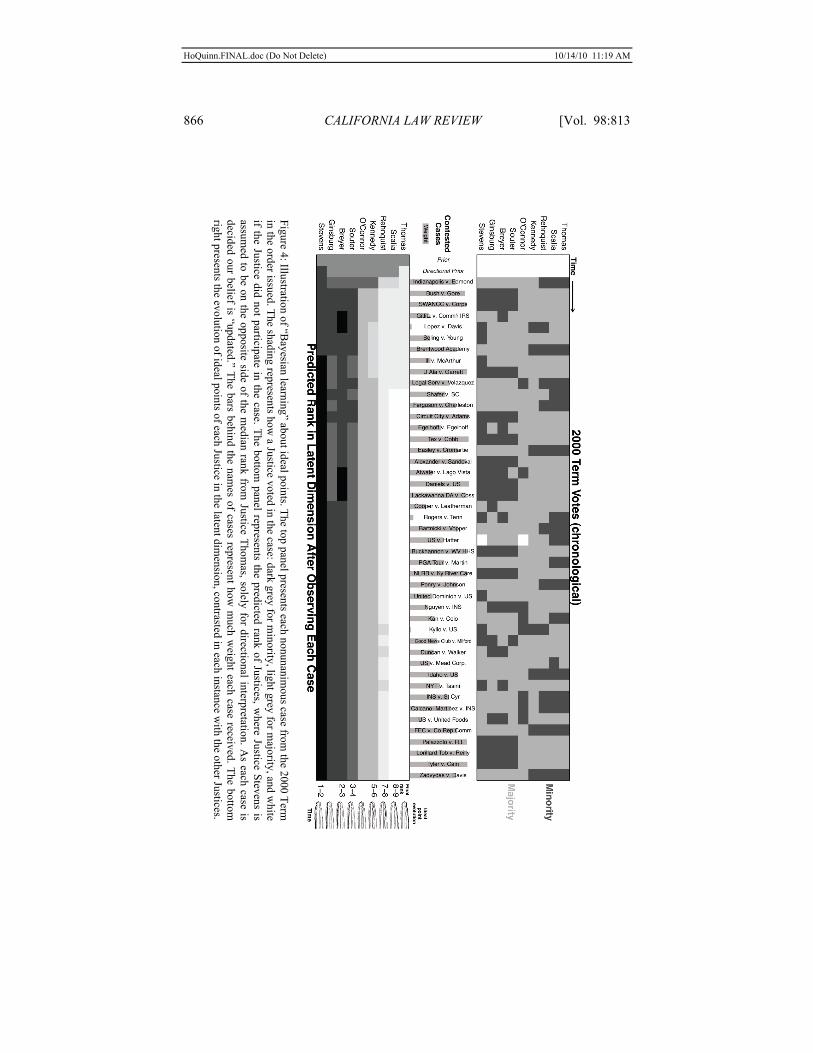
HoQuinn.FINAL.doc (Do Not Delete) 10/14/10 11:19 AM
866 CALIFORNIA LAW REVIEW [Vol. 98:813
Figure 4: Illustration of “Bayesian learning” about ideal points. The top panel presents each nonunanim
ous case from the 2000 Term
in the order issued. The shading represents how
a Justice voted in the case: dark grey for minority, light grey for m
ajority, and white
if the Justice did not participate in the case. The bottom panel represents the predicted rank of Justices, w
here Justice Stevens is assum
ed to be on the opposite side of the median rank from
Justice Thomas, solely for directional interpretation. A
s each case is decided our belief is “updated.” The bars behind the nam
es of cases represent how m
uch weight each case received. The bottom
right presents the evolution of ideal points of each Justice in the latent dim
ension, contrasted in each instance with the other Justices.

HoQuinn.FINAL.doc (Do Not Delete) 10/14/10 11:19 AM
2010] HOW NOT TO LIE WITH JUDICIAL VOTES 867
Figure 5: Illustration of the ideal points of Justices on the Rehnquist C
ourt. The left panel presents the estim
ated locations of Justices in the latent dimension. V
ertical segments represent the best guess
of the location (posterior medians), and horizontal segm
ents represent 95 percent uncertainty intervals. The strip below
plots the estimated cutlines separating the m
ajority and minority for all
nonunanimous decisions. U
sing the notation in Ho &
Quinn, View
point Diversity, supra note 15, at
866–68, the cutting lines represent the posterior median α divided by the posterior m
edian β (i.e., the estim
ated point in latent space where the probability of voting for the m
ajority and minority is 0.5).
The cutlines illustrate that the primary inference is about the relative and not absolute position of the
Justices: the right-skewed m
arginal distribution of ideal points matches the sim
ilar skew of cutlines.
The red cluster represents the conventional 5–4 split on the Rehnquist C
ourt. The right panel presents the probability of ranks for each Justice. For each Justice, the probability of occupying the rank in the order presented is greater than 0.85.

HoQuinn.FINAL.doc (Do Not Delete) 10/14/10 11:19 AM
868 CALIFORNIA LAW REVIEW [Vol. 98:813
Figure 6: Supreme C
ourt ideal points over time (1921–2006). Large red dots indicate start of service (or observation period) for each
Justice, and red lines trace period of service. Small blue dots represent cutpoints (w
hich represent the same m
odel as in Figure 5) that m
odel the voting splits on all contested issues. Ideal points are transformed to a logistic scale—
the logistic transformation of x is 1/(1
+ exp(-x))—in order to increase the visibility of Justices falling in the m
id-range of the latent dimension.

HoQuinn.FINAL.doc (Do Not Delete) 10/14/10 11:19 AM
2010] HOW NOT TO LIE WITH JUDICIAL VOTES 869
Figure 7: Illustration of temporal sm
oothing to assess preference change over time. The “sm
oothing” parameter τ ranges from
0 to ∞
, with 0 representing com
plete pooling and ∞ representing no pooling. This figure dem
onstrates that moderate pooling can help
show changes in ideal points over tim
e. The top left panel presents hypothetical ideal points for a single Justice estimated separately
for each Term. The top right panel w
eakly pools these Terms, and the bottom
left panel moderately pools these cases. The bottom
right panel com
pletely pools Terms, such that a single ideal point is estim
ated across all Terms, as in Figure 6.

HoQuinn.FINAL.doc (Do Not Delete) 10/14/10 11:19 AM
870 CALIFORNIA LAW REVIEW [Vol. 98:813
Figure 8: Evolution of Justice Blackmun over time. The estimated position of Justice Blackmun in each Term is given by the blue line and light blue 95 percent uncertainty band. The scale is logit-transformed for visibility. The panels also display the ideal point trajectories of the other Justices serving during this time period. The right panel also displays the estimated cutpoints. Cutpoints between Justices White and Blackmun appear red whenever Justice Blackmun is above Justice White. Cutpoints between Justices White and Blackmun appear green whenever Justice Blackmun is below Justice White.
Figure 9: The dangers of extrapolation. The left panel plots the estimated ideal points, assumed to be temporally constant, of Justices McReynolds, Frankfurter, and Brandeis, along with the cutpoint from Bush v. Gore. Lines in black correspond to the actual terms of service for these Justices. The grey lines extrapolate out to the 2000 Term of the Court. The right panel demonstrates just how sensitive inferences can be to extrapolation by plotting data on the winning times in the Olympic 100-meter dash for both men and women. Applying linear regression models (the solid lines) to these data suggests that in 2156 female sprinters will be faster than male sprinters. Tatem, supra note 94, at 525. Note, however, that quadratic models fit the observed data almost identically but that these fits suggest that both male and female sprinters will become much slower in the future.
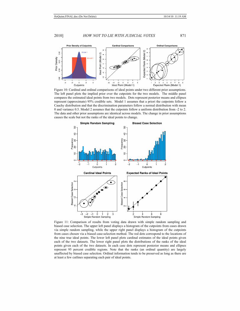
HoQuinn.FINAL.doc (Do Not Delete) 10/14/10 11:19 AM
2010] HOW NOT TO LIE WITH JUDICIAL VOTES 871
Figure 10: Cardinal and ordinal comparisons of ideal points under two different prior assumptions. The left panel plots the implied prior over the cutpoints for the two models. The middle panel compares the estimated ideal points from two models. Dots represent posterior means and ellipses represent (approximate) 95% credible sets. Model 1 assumes that a priori the cutpoints follow a Cauchy distribution and that the discrimination parameters follow a normal distribution with mean 0 and variance 0.5. Model 2 assumes that the cutpoints follow a uniform distribution from -2 to 2. The data and other prior assumptions are identical across models. The change in prior assumptions causes the scale but not the ranks of the ideal points to change.
Figure 11: Comparison of results from voting data drawn with simple random sampling and biased case selection. The upper left panel displays a histogram of the cutpoints from cases drawn via simple random sampling, while the upper right panel displays a histogram of the cutpoints from cases chosen via a biased case-selection method. The red dots correspond to the locations of the nine true ideal points. The lower left panel plots cardinal estimates of the ideal points given each of the two datasets. The lower right panel plots the distributions of the ranks of the ideal points given each of the two datasets. In each case dots represent posterior means and ellipses represent 95 percent credible regions. Note that the ranks (an ordinal quantity) are largely unaffected by biased case selection. Ordinal information tends to be preserved as long as there are at least a few cutlines separating each pair of ideal points.

HoQuinn.FINAL.doc (Do Not Delete) 10/14/10 11:19 AM
872 CALIFORNIA LAW REVIEW [Vol. 98:813
Figure 12: Com
parison of conventional numerical representation of Lujan v. D
efenders of Wildlife, 504 U
.S. 555 (1992), in the Suprem
e Court D
atabase on the left panel and a more nuanced representation on the right panel, w
hich disaggregates the merits and
discrete standing issues.

HoQuinn.FINAL.doc (Do Not Delete) 10/14/10 11:19 AM
2010] HOW NOT TO LIE WITH JUDICIAL VOTES 873
Figure 13: Term-by-Term
ideal point estimates for the 1931–40 Term
s of the Court. The left panel presents results from
separate m
odels fit to each Term, so that the estim
ates are not anchored across time in any m
eaningful way. G
rey lines represent all Justices serving during those Term
s and the dark line (with shaded 95 percent uncertainty interval) represents Justice R
oberts, w
ho is hypothesized to have shifted sharply from the 1935 Term
to the 1936 Term (the vertical grey period). The m
iddle panel anchors the estim
ates by assuming Justice Stone to be constant. Justice R
oberts shifts sharply during the 1936 Term. The right
panel assumes that Justice R
oberts’s position is constant over time and depicts the other Justices in black. U
nder this assumption
all other Justices—save for Justice H
ughes, who is also posited to have shifted—
shift sharply in the opposite direction. These estim
ates provide strong evidence for the switch in tim
e. See Ho &
Quinn, Sw
itch in Time, supra note 15.

HoQuinn.FINAL.doc (Do Not Delete) 10/14/10 11:19 AM
874 CALIFORNIA LAW REVIEW [Vol. 98:813
Figure 14: Illustration of relationship between unidim
ensional and two-dim
ensional ideal point results.The left panel plots the two-
dimensional posterior m
eans and approximate 95 percent credible regions for ideal points from
an analysis of all voting blocs in the last natural R
ehnquist Court. The m
iddle panel plots the two-dim
ensional ideal points from the left panel along w
ith the cutlines from
votes
that feature
perfect unidim
ensional spatial
voting (based
on the
unidimensional
ordering described
above). A
pproximately 43 percent of the voting blocs feature such perfect spatial voting. The right panel displays the cutlines from
votes that did not feature perfect unidim
ensional spatial voting. The cutlines in the middle panel fan out radially from
the bottom center,
indicating that the unidimensional space lies on a curve inside the tw
o-dimensional space. The cutlines in the right panel do not
exhibit any clear structure, suggesting that improved fit of the tw
o-dimensional m
odel is largely the result of the model capturing
idiosyncratic voting patterns.

HoQuinn.FINAL.doc (Do Not Delete) 10/14/10 11:19 AM
2010] HOW NOT TO LIE WITH JUDICIAL VOTES 875
Figure 15: Reversal in merits-standing preferences over time. The panels present pooled merits ideal points on the x-axis against the proportion of votes cast by each Justice favoring standing in contested cases from pre-1940 and post-1940 cases, respectively. The area of each observation is proportional to the number of issues. To account for measurement uncertainty, the superimposed lines represent regression lines fit to the data from fifty draws of the posterior distribution of merits ideal points. See Ho & Ross, supra note 15, at 33.
Figure 16: Comparison of the ability to correctly classify votes on cases containing the Westlaw Key Number Statutory Construction and Operation (361VI) relative to the null distribution formed from all nonunanimous cases in a Term. A simple unidimensional dynamic ideal point model classified the votes. Note that votes on statutory cases were much more difficult to predict than other case votes during the period from roughly 1955 to 1990.

HoQuinn.FINAL.doc (Do Not Delete) 10/14/10 11:19 AM
876 CALIFORNIA LAW REVIEW [Vol. 98:813
Figure 17: Model-based measurement of backlash. The blue text plots the Justice votes in each case, while the red text plots the newspaper editorial board positions. For example, the New York Times (NYT), located in the lower left hand corner of the left panel, opined against the majority in Printz v. United States. The blue curves present probability models of a majority vote from the Justices alone. The red curves present probability models pooling both Justices and newspaper positions, where the Justice positions are the same in the latent dimension. The left panel illustrates the typical case, where newspapers and Justices adopt positions in predictable ways. The right panel illustrates a model-based method of assessing backlash: while the Justices split 5-4 in Atwater v. City of Lago Vista, every newspaper from across the spectrum opined in favor of the minority. The divergence between the curves detects such differential behavior.