0

HOW MUCH DO THE TAX BENEFITS OF DEBT ADD TO FIRM VA LUE?: EVIDENCE FROM SPANISH LISTED FIRMS

José A. Clemente-Almendros

Departamento de Economía y Empresa

Universidad CEU Cardenal Herrera

Francisco Sogorb-Mira

Departamento de Economía y Empresa

Universidad CEU Cardenal Herrera

This version: April 2015

Area thematic : b) VALORACIÓN Y FINANZAS

Keywords : Capital Structure, Corporate Taxes, Marginal Tax Rate, Debt Tax Shield.

JEL Classification : G32, H25

____________________________________

Francisco Sogorb-Mira acknowledges financial support from Ministry of Economy and Competitiveness research grant ECO2012-34268. Any errors are our sole responsibility.

47b

1

HOW MUCH DO THE TAX BENEFITS OF DEBT ADD TO FIRM VA LUE?: EVIDENCE FROM SPANISH LISTED FIRMS

Abstract

It is generally recognized that taxation has potentially important impact on corporate

financing decisions. Nevertheless, the empirical evidence is far from conclusive. In this

study, we assess the debt tax benefits of Spanish listed firms throughout the period

2007-2013. Specifically, we found the capitalized value of gross interest deductions

mounts to approximately 6.4% of market value, while the debt net (of personal taxes)

benefit estimated is 2.1%, in contrast to the traditional 11.4% (marginal tax rate times

debt). As a different approach, we also use panel data linear and nonlinear regressions

to estimate the value of the debt tax benefit. Our evidences support the view that taxes

are important for corporate decision-making and that debt contributes to firm value

¿CUÁNTO APORTAN / CONTRIBUYEN LOS BENEFICIOS FISCA LES DE LA DEUDA AL VALOR EMPRESARIAL? EVIDENCIA DE EMPRESAS C OTIZADAS

ESPAÑOLAS

Resumen

Existe un vasto reconocimiento acerca de que los impuestos tienen un impacto

potencial importante en las decisiones financieras empresariales. Sin embargo, la

evidencia empírica está lejos de ser concluyente. En este estudio, valoramos los

beneficios fiscales de la deuda para empresas cotizadas españolas durante el período

2007-2013. Concretamente, encontramos que el valor actualizado de la deducción

bruta de los intereses de la deuda supone aproximadamente el 6,4% del valor de

mercado de la empresa, mientras que el beneficio de la deuda neto (de impuestos

personales) estimado es del 2.1%, en comparación con el valor más tradicional del

11.4% (resultado de multiplicar el tipo impositivo marginal por el nivel de deuda). Como

enfoque diferente, también usamos regresiones lineales y no lineales de datos panel

para estimar el valor de los beneficios fiscales de la deuda. Nuestra evidencia apoya la

idea de que los impuestos son importantes para la adopción de decisiones en las

empresas y que la deuda contribuye al valor empresarial.

2

1. Introduction

The tax benefits of debt are the tax savings that result from deducting interest from

taxable earnings. By deducting one euro of interest, a firm reduces its tax liability by the

marginal corporate tax rate. Since Modigliani and Miller (1963) hypothesized that the

tax benefits of debt increase firm´s value, the implications of debt tax shield on firm

valuation and capital structure has attracted attention as well as debate among the

financial community. Nevertheless, how much is that increase in firm value?

Different approaches have generated controversial on the implicit benefits of debt. For

instance, Miller (1977) pointed out that personal taxes might compensate the tax

benefit of debt. Besides, Fama and French (1998) maintained that it remains unclear

as to whether debt tax shields improve firm´s value, and found a significant negative

relationship between debt and firm´s value, contrary to expectations. They attributed

the findings of positive relationships in previous research, to potential failure to control

for profitability. In an effort to avoid this problem, Kemsley and Nissim (2002) ran

reverse regressions of profitability on firm´s value and debt, and found significant tax

benefits of debt. Furthermore, Graham (2000) used firm-level financial statement data

and proved that firms derive substantial tax benefits from debt. More recently, Blouin,

Core and Guay (2010), have stated that the tax benefits of debt might be smaller than

previously suggested, due to a biased estimation of marginal tax rates.

Nowadays, the assessment of debt tax shield has raised in importance, due to

circumstances such as the large increase in the corporate borrowing, the generalized

trend in changes in tax codes throughout the world, and finally the growing importance

of valuation in corporate transactions such as M&As, Venture Capital, etc. (Cooper and

Nyborg, 2007). Notwithstanding its implications, there is still not unanimous consensus

about which the relevance of debt tax shield concerns. As Graham (2008) states, the

evidence consistent with tax benefits adding to firm value is ambiguous because non-

tax explanations or econometric issues might cloud interpretation. In this sense,

additional cross-sectional and/or panel data regression research, that investigates the

market value of the tax benefits of debt, would be helpful in terms of clarifying or

confirming the interpretation of existing cross-sectional regression analysis.

Accordingly, the main purpose of this study is to estimate the value of the debt tax

shield of Spanish listed companies for the period 2007-2013. Specifically, we calculate

3

corporate marginal tax rates to simulate the interest deduction benefit functions for

individual firms, and use them to estimate the tax-reducing value of each incremental

euro of interest expense as in Graham (2000). Besides, we also estimate reverse

regressions in which we regress future profitability on debt following Kemsley and

Nissim (2002) approach. This estimation procedure allows coping with the potential

correlation between debt and the value of operations along nontax dimensions such as

growth, financial distress and size.

Our findings clearly show that there is a clear fiscal advantage of using debt financing.

In our sample, we find the tax benefit of debt equals 6.4 per cent of firm value, meaning

that the median firm at its leverage ratio is worth in this percentage more than the same

firm with no debt in its capital structure. After accounting for reductions for personal

taxes, we find that the tax benefit of debt under the marginal benefit curve is 2.1 per

cent of firm value. Under a regression approach, the net debt tax shield mounts up to

11.2 per cent of firm value.

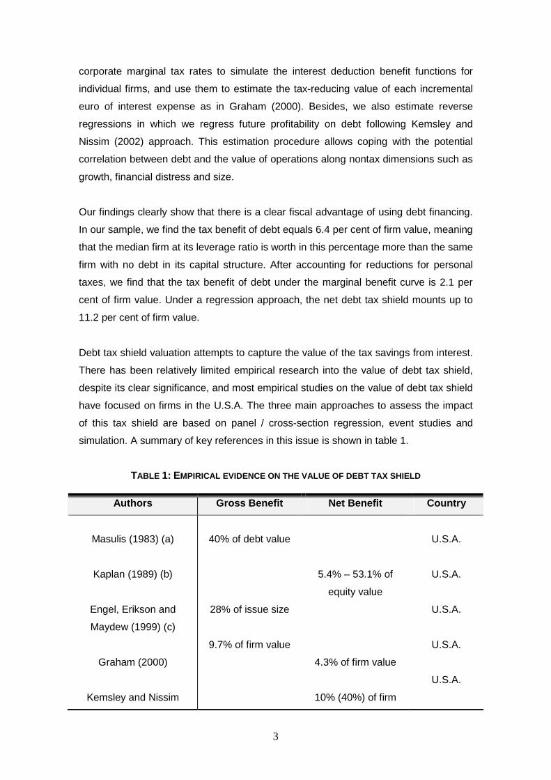
Debt tax shield valuation attempts to capture the value of the tax savings from interest.

There has been relatively limited empirical research into the value of debt tax shield,

despite its clear significance, and most empirical studies on the value of debt tax shield

have focused on firms in the U.S.A. The three main approaches to assess the impact

of this tax shield are based on panel / cross-section regression, event studies and

simulation. A summary of key references in this issue is shown in table 1.

TABLE 1: EMPIRICAL EVIDENCE ON THE VALUE OF DEBT TAX SHIELD

Authors Gross Benefit Net Benefit Country

Masulis (1983) (a)

Kaplan (1989) (b)

Engel, Erikson and

Maydew (1999) (c)

Graham (2000)

Kemsley and Nissim

40% of debt value

28% of issue size

9.7% of firm value

5.4% – 53.1% of

equity value

4.3% of firm value

10% (40%) of firm

U.S.A.

U.S.A.

U.S.A.

U.S.A.

U.S.A.

4

(2002)

Korteweg (2010)

Van Binsbergen et al.

(2010) (d)

Ko and Yon (2011) (e)

Sarkar (2014)

Doidge and Dyck (2015)

3.5% of asset value

5.2% (5.5%) of firm

value

0.6% - 7.2% of

equity value

4.6% of firm value

(debt) value

5.5% of firm value

1.9% (2.0%) of firm

value

U.S.A.

U.S.A.

Korea

U.S.A.

Canada

(a) He regressed stock returns on the change in debt in exchange offers, and found a debt coefficient statistically indistinguishable from the top statutory corporate tax rate at that era; (b) the lower estimates assume that leveraged buyout debt is repaid in eight years and that personal taxes offset the benefit of corporate tax deductions. Conversely, the higher estimates assume that leveraged buyout debt is permanent and that personal taxes provide no offset; (c) they examined a capital structure transaction involving two securities that were nearly identical except for their tax treatment, namely trust preferred stock and traditional preferred stock; (d) they simulated tax benefit functions using Graham (2000) approach; (e) the estimates are based upon Graham (2000) (Blouin et al., 2010) simulation approach.

The literature of the debt tax shield has produced a wide range of estimates, some of

which are subject to non-tax explanations or identification challenges1. For example,

Graham (2000) found that the gross tax benefit of debt is worth 9.7% for firm value,

whereas Korteweg (2010) and Van Binsbergen, Graham and Yang (2010) obtained

5.5% and 3.5%, respectively. On the other hand, Kemsley and Nissim (2002) estimated

a net benefit to debt of 10% (40%) of firm (debt) value; though consistent with Masulis

(1983), such large coefficients imply near-zero average debt costs and a near-zero

effect of personal taxes (Graham, 2008 and 2013). In countries other than the U.S., Ko

and Yon (2011) conducted an analysis using a data panel on Korean firms and found a

gross debt benefit of 5.2% of firm value. In addition, Doidge and Dyck (2015) obtained

a 4.6% of firm value for Canadian firms. To the best of our knowledge, no empirical

study has been carried out on this matter so far, specifically in Spain or generally in

Europe.

1 A comprehensive survey of related literature can be found in Graham (2003), Graham (2008), Graham (2013) and Hanlon and Heitzman (2010).

5

Our study contributes to the literature in several respects. First, we find new results on

the estimation of the value of tax shields comparing two approaches, namely simulation

and regression approaches. Furthermore, we provide empirical evidence within a

European context for the first time, and specifically for Spanish firms. Second, we use

panel data econometrics for our regression approach combining linear and non-linear

estimations, and thus exploiting the most our data. Third, the findings of the present

study demonstrate that though the fiscal benefits of debt are relevant, they are also

sensitive to the valuation approach chosen.

The remainder of the paper is organized as follows. In the next section, we discuss the

simulation approach based on Graham (2000) simulation procedure, while Section 3

deals with the regression approach which grounds upon Kemsley and Nissim (2002)

proposals. Section 4 presents the data for the study and the descriptive analysis

regarding the key variables. The empirical results are discussed in Section 5. Several

robustness tests are presented in Section 6 and the final section provides some

concluding remarks.

2. Simulation approach

2.1. The value of the debt tax benefit

The value of the debt tax shield is the present value of the tax savings from interest

expense (Cooper and Nyborg, 2006). In a Modigliani and Miller (1963) context, that is

with perpetual debt and if interest tax shields are completely utilized, the capitalized tax

benefit of debt can be simplified to the marginal corporate tax rate times the amount of

debt. That is,

c d

d

t r D

r

⋅ ⋅ [1]

Where tc is the marginal corporate tax rate, rd is the interest rate on debt and D is the

amount of debt.

An important question with this approach is that it does not consider personal income

taxes, as pointed out by Miller (1977). With personal taxes, the capitalized tax benefit

of debt can be computed as follows,

6

( ) ( ) ( )( )

p c e d

p d

1 t 1 t 1 t r D

1 t r

− − − ⋅ − ⋅ ⋅

− ⋅ [2]

Where tp and te are both marginal personal tax rates that are applied to interest´s and

equity´s incomes, respectively. Note that if both tp and te are zero (or they are equal),

then Equation [2] is simplified to the Modigliani and Miller (1963) set up (i.e. Equation

[1]).

Equity income includes both dividends and capital gains. The personal marginal tax

rates on these income streams may differ, and capital gains tax could be deferred by

investors not realizing the gains. Therefore, the marginal personal equity tax rate

should be a mixture of dividends and capital gains tax rates. Following Gordon and

Mackie-Mason (1990), the personal equity tax rate might be calculated as:

e p pt d t (1 d) t γ= ⋅ + − ⋅ ⋅ [3]

Where d is the dividend pay-out ratio and γ is an adjustment factor that takes into

account the possible deferral of taxes on capital gains and the time value of money of

the capitalized taxes2.

Graham (2000, 2001) simulates interest deduction benefit functions and uses them to

estimate the tax-reducing value of each incremental euro of interest expense. The

estimation of the tax benefits of debt is carried out by integrating the area under the tax

benefit function, which relates marginal tax rates to interest deductions. The process of

making up the tax benefit function follows different stages. Firstly, MTRit0% is estimated

for firm i in year t3. This is the marginal tax rate based on taxable income assuming the

firm has zero debt and therefore no interest deductions. Secondly, new marginal tax

rates are estimated with different percentages (p%) of the actual interests paid:

MTRitp%, where p% ranges from 20% to 800%4. Thirdly, the firm´s tax benefit function

is derived by connecting the previous estimated marginal tax rates with each level of

interest.

2 This adjustment factor is established at 0.25 following Gordon and Mackie-Mason (1990), Graham (1999), Graham (2000), and Green and Hollifield (2003). 3 As in Graham, Lemmon and Schallheim (1998), we estimate marginal tax rates with pre-financing earnings and assuming that EBIT follows a pseudo-random walk process with a drift (see Clemente-Almendros and Sogorb-Mira, 2015, for details). 4 The exact numbers are 20%, 40%, 60%, 80%, 100%, 120%, 160%, 200%, 300%, 400%, 500% 600%, 700% and 800%.

7

Marginal tax benefits of debt decline as more debt is added because the probability

increases with each incremental euro of interest that it will not be fully valued in every

state of the world. Figure 1 depicts an example of the tax benefit function throughout

different years for a representative firm of our sample, namely, Meliá Hotel

International, S.A. (MEL).

FIGURE 1: TAX BENEFIT FUNCTION FOR MELIÁ HOTELS INTERNATIONAL , S.A. (MEL)

The integration of the area under the tax benefit curve up to the level of actual interest

expense leads to the debt tax benefit. For each year and for each firm, we measure the

area under the firm´s tax benefit function up to 100% of annual interest multiplied by

actual interest payments to determine firm´s annual debt tax shield. Then, we estimate

the capitalized tax benefits of debt under the assumption that the debt tax shield

computed at the end of year t will be maintained over the following years. The interest

rate on debt for each firm, computed as the quotient between interest expenses and

debt, is used as the discount rate. Finally, we evaluate firm value as the sum of market

value of equity and book value of financial debt.

2.2. The kink

8

Graham (2000) offers an empirical measure of the underutilization of debt by

companies and calls this measure the kink. It is defined as the maximum amount of

interest deductions a firm could charge, before any decline in the marginal tax benefit

of debt relative to the actual interest charge the firm incurred given its current debt. In

short, it is the point at which the tax benefit curve starts to slope downwards. We fix the

magnitude of the decline in the tax benefit curve at 25 basis points5. The use of debt to

minimize tax paying leads to classify firms´ debt policy as aggressive or conservative.

Accordingly, an aggressive firm with positive earnings before interest and taxes would

issue just enough debt to ensure that earnings after interest but before taxes are zero,

whereas a conservative firm would issue less debt and therefore face positive taxes.

As a result, a firm´s debt financing policy could be considered as aggressive

(conservative) when its kink is smaller (larger) than one6.

The kink could be computed as a ratio where the numerator is the maximum interest

that could be deducted for tax purposes before expected marginal benefits begin to

declines, and the denominator is actual interest incurred (Caskey, Hughes and Liu,

2012):

Target InterestKink=

Actual Interest [4]

Where Target Interest is the point at which the firm´s tax benefit function starts to slope

down as the firm uses more debt.

Figure 2 shows the tax benefit functions of two example firms, namely, Telefónica, S.A.

(TEF) and Actividades de Construcción y Servicios, S.A. (ACS).

FIGURE 2: THE KINK FOR TELEFÓNICA, S.A. (TEF) AND ACTIVIDADES DE CONSTRUCCIÓN Y SERVICIOS, S.A. (ACS)

5 Graham (2000), Blouin et al. (2010) and Van Binsbergen et al. (2010) define the kink as the first interest increment at which the firm has a decline in its marginal tax rate of at least 50 basis points. We decided to lessen this requirement in order to capture more variability in our data. 6 This characterization is based on the tax benefit of debt without considering its cost. Therefore, an aggressive-conservative debt policy in this context does not necessarily imply sub-optimality.

9

For example, in year 2013, although the tax benefit curve of TEF declines from 80% of

the actual interest (i.e. kink of 0.8), that of ACS kinks at 160% (i.e. kink of 1.6). In this

case, the kink of TEF denotes that the firm´s incremental interest generates marginal

tax benefits smaller than what the firm has received from its current interest. On the

other hand, for ACS, even when interest payments multiply by 1.6 times, the firm could

still enjoy tax benefits at the marginal tax rate. ACS will remain at the flat part of its tax

benefit curve even if it increases debt to 160% of the current level.

Underleveraged firms loose significant tax savings, that otherwise would have been

available if they had increased their debt levels to their kink. Nevertheless, Graham

(2000) maintains that firms with large kinks should remain on the flat part of their tax

benefit functions, even when their income declines, in order to be called “conservative”

in terms of their debt usage. Besides, if two “conservative” firms have the same kink

but one has more volatile earnings than the other, then the former firm has a less

conservative policy since the probability of being in the downward sloping part of the

tax benefit function (aggressive debt policy) in the future is higher for this firm than for

the firm with lower volatility. Accordingly, it is necessary to calculate a new measure of

the kink to account for this fact. Following Graham (2000), this complementary kink

measure called standardized kink, will reflect the length of the flat part of the tax benefit

10

function per unit of income volatility. Specifically, we compute this standardized

measure of the kink as,

Interest Expense at the KinkStandardized Kink=

Standard Deviation of EBIT [5]

2.3. Zero tax benefit of debt

We identify the level of interest expense at which the tax benefit of debt becomes zero,

and called it ZeroBen.

Figure 3 displays the tax benefit functions of two example firms, namely, Fomento de

Construcciones y Contratas, S.A. (FCC) and Fluidra, S.A. (FDR).

FIGURE 3: ZEROBEN FOR FOMENTO DE CONSTRUCCIONES Y CONTRATAS , S.A. (FCC) AND FLUIDRA, S.A. (FDR)

For year 2013, ZeroBen are 700% and 400% for FCC and FDR, respectively. The

economic interpretation of these figures is that FCC and FDR could use seven and four

times, respectively, their actual interest before the marginal benefit reaches zero level.

11

3. Regression approach

3.1. Forward specification

Considering corporate taxes, Modigliani and Miller (1963) established the valuation of a

leveraged firm as follows,

L U cV V t D= + ⋅ [6]

Where VL is the market value of the leveraged firm, VU is the market value of the

unleveraged firm, tc is the corporate marginal tax rate and D is the debt level.

If we also take into account personal taxes, Equation [6] will still be valid; although

corporate marginal tax rate shall we substituted by a mixture of corporate and personal

tax rates as explained in Miller (1977). That is,

c eL U

p

(1 t ) (1 t )V V 1 D

(1 t )

− ⋅ −= + − ⋅ − [6 bis]

Where te and tp are both marginal personal tax rates that are applied to equity´s and

interest´s incomes, respectively.

Fama and French (1998) suggested estimating Equation [6] by regressing VL on debt

interest, dividends, and a proxy of VU. Specifically, they measured VL as the excess of

market value over book assets, and proxied VU with several control variables such as

current earnings, assets and R&D expenses, as well as future changes in these same

variables7. A positive coefficient on the interest explanatory variable shall be evidence

of positive tax benefits of debt. Contrary to expectations, Fama and French (1998)

found in their regressions either non-significant or negative estimated coefficients on

interest. As a result, they interpreted this evidence as being inconsistent with debt tax

benefits having a first-order effect on firm value. They justified this antagonic evidence

with a mismeasurement of VU, and the interest variable including information about

earnings not captured by control variables.

7 All the regression variables were deflated by total assets.

12

Kemsley and Nissim (2002) endeavoured to bypass the VU measurement problem with

two alternative proposals. In the first one, they proxied VU with the present value of the

expected operating income,

cU

E(FOI) E(EBIT (1 t ))V

ρ ρ

⋅ −= = [7]

Where E() is the expected operator, FOI is future operating income, EBIT is earnings

before interest and taxes8, and ρ is the capitalization rate.

Combining Equations [6] and [7], we derive:

L c

E(FOI)V t D

ρ= + ⋅ [8]

And from Equation [8], the following model specification is developed:

itL 0 1 2 it it

it

E(FOI)V β β β D ε

ρ= + ⋅ + ⋅ + [9]

Where β2 represents the estimated value for the debt tax shield.

Model coming from Equation [9] has two drawbacks. First, debt is likely to be correlated

with the value of operations (i.e. E(FOI) and ρ) along several nontax dimensions, and

therefore β2 would be biased. Second, using the market value of the firm as the

dependent variable instead of the market-to-book ratio might preclude considering risk

issues related to ρ and expectations about growth in operating income. Consequently,

Kemsley and Nissim (2002) suggest a second alternative to the forward specification,

called the reverse specification, in order to circumvent the measurement problems.

Empirical estimation of Equation [9] implies some kind of assumptions about expected

future earnings (E(FOI)) and the capitalization rate (ρ). Specifically, we proxy E(FOI) as

EBIT times one minus marginal corporate tax rate. Conversely, we consider ρ as a

constant and hence we do not include any specific controls for the capitalization rate.

Following Kemsley and Nissim (2002) we deflate the intercept and all explanatory

8 The use of EBIT as the basic of valuation is strictly valid only when the underlying real assets are assumed to have perpetual lives. In such a case, EBIT and cash flow are one and the same (Modigliani and Miller, 1963).

13

variables by total assets in order to handle heteroskedasticity9. Consequently, the

empirical specification of Equation [9] now resembles the following,

itL 0 it it1 2 it

it it it it

V β E(FOI) Dβ β ε

Total Assets Total Assets Total Assets Total Assets= + ⋅ + ⋅ + [10]

3.2. Reverse specification

The reverse specification proposal consists in performing a switch of variables in

Equation [6], moving VU to the left-hand side and VL to the right-hand side of the

equation. The resulting relation is:

U LV V coefficient D= − ⋅ [11]

Now, adopting Equation [8] in the same spirit of Equation [11], and operating for

E(FOI),

L cE(FOI) ρ (V t D)= ⋅ − ⋅ [12]

Finally, from Equation [12] we derive the following specification model:

itit 0 1 it L 2 it itE(FOI) β β ρ (V β D ) ε= + ⋅ ⋅ − ⋅ + [13]

Where β2 represents the estimated value for the debt tax shield.

Model of Equation [13] overcomes the two limitations of the forward model. First,

placing E(FOI) on the left-hand side of [13] transfers the measurement error in the

proxy for E(FOI) to the dependent variable, and in this sense the regression residual

can capture the random component of the error. Second, moving VL to the right-hand

side of Equation [13] controls for all market information concerning expected operating

earnings and ρ.

9 Fama and French (1998) deflated all the explanatory variables but not the intercept. This choice implies that all regression variables in Equation [10] are converted into ratios.

14

Equation [13] shows a non-linear relationship among the parameters, and there are

basically two ways to estimate it: by using a linear transformation of the equation and

by using nonlinear least squares (Hoaglin, 2003; McGuirre et al., 2014). If we consider

ρ as a constant and deflate the intercept and all the explanatory variables by total

assets, we can set up the following linear specification of Equation [13],

it 0 Lit it1 2 it

it it it it

E(FOI) β V Dβ β ε

Total Assets Total Assets Total Assets Total Assets= + ⋅ + ⋅ + [14]

In this method the estimate for the debt tax shield is calculated as the quotient between

–β2 and β1. Using market value as an explanatory variable allows us to control for ρ,

but nevertheless we need to assume market efficiency (Penman, 1996). On the other

hand, we need a proxy for expected future earnings and as in the forward specification,

we use EBIT times one minus marginal corporate tax rate.

The second way of estimating Equation [13] is carrying it out directly by nonlinear least

squares. Now, instead of considering ρ as a constant, we express the capitalization

rate as a linear function of several observable instruments associated with risk and

growth. Specifically, we use four variables namely the industry median beta of

operations (βU) (Modigliani and Miller, 1966); the market-to-book ratio of operations or

the quotient between the market value of operations (VL – β D) and net operating

assets (NOA) (Fama and French, 1992, and Penman, 1996); size measured as the

natural logarithm of NOA; and the natural logarithm of operating liabilities (OL)

(Hoaglin, 2003, and McGuirre et al., 2014). To control for any direct relation between

E(FOI) and the abovementioned variables, we also include these variables in additive

form in the regression (Kemsley and Nissim, 2002). Finally, to control for industry

effects, we replace the intercept in Equation [13] with industry dummies. As a result, we

come up with the next empirical specification:

( ) ( ) ( )

( ) ( )

Lit itit 0 1 U 2 3 4 Lit itit it

it

8Lit it

1i i 2 3 4 itit iti 1 it

V β DE(FOI) β β β β β ln NOA β ln OL V β D

NOA

V β Dγ Dummy_Industry γ γ ln NOA γ ln OL ε

NOA=

− ⋅= + ⋅ + ⋅ + ⋅ + ⋅ ⋅ − ⋅ +

− ⋅+ ⋅ + ⋅ + ⋅ + ⋅ +∑ [15]

15

The net tax benefit from a euro of debt, i.e. the debt tax shield, is represented by β.

Equation [15] is estimated using nonlinear least-squares as it is nonlinear in the

parameters. To alleviate possible effects of heteroskedasticity, we weight the

observations by the reciprocal of the square of total assets, which is consistent with

deflating the entire equation by total assets.

4. Data and descriptive statistics

4.1. Sample selection

The data used in this paper come from four sources. The Sistema de Análisis de

Balances Ibéricos (SABI), a database managed by Bureau Van Dijk and Informa D&B,

S.A., and the Spanish Securities and Exchange Commission, i.e. CNMV, provide the

accounting information from annual accounts, while financial market information comes

from the quotation bulletins of the Spanish Stock Exchange and Bloomberg.

As it is standard in the empirical literature, financial institutions, utilities and

governmental enterprises are disregarded because these types of companies are

intrinsically different in the nature of their operations and financial accounting

information. We also excluded companies with negative equity, i.e. near bankruptcy

firms. Overall, we have a balanced data panel containing 88 companies with a total of

616 observations. In order to mitigate the effect of outliers, all variables are winsorised

at 0.5% in each tail of the distribution.

4.2. Descriptive statistics

Table 2 presents summary statistics for the simulation approach tax variables (Panel A)

joint with the regression approach key variables (Panel B).

TABLE 2: DESCRIPTIVE STATISTICS*

Variables Mean Median St. Dev. Min. Max.

PANEL A

MTR0% 0.1784 0.1910 0.0824 0.0002 0.3000

MTR100% 0.1737 0.1879 0.0840 0.0003 0.3000

Kink 3.0765 1.0000 3.2265 0.0000 8.0000

16

ZeroBen 7.9100 8.0000 0.5697 2.0000 8.0000

PANEL B

VL 1.6302 1.1687 1.5939 0.2043 11.6750

OI 0.0299 0.0241 0.0772 -0.3506 0.3919

NOA 1.0552 0.9310 1.9869 0.1800 23.7903

OL 0.1398 0.0718 0.1757 0.0009 0.8200

βU 0.4812 0.4204 0.3382 -0.0775 1.4212

D 0.3497 0.3222 0.2293 0 0.9202

*Table A1 in the Appendix provides definitions of all the variables. VL, OI, NOA, OL and D are all deflated by total assets.

From Panel A of Table 2, we observe that the mean value of the before-financing

marginal tax rate is 17.37% (17.84% assuming the firm has no interest deductions),

with a maximum value of 30% (maximum value for the statutory tax rate) and a

standard deviation of 8.40% (8.24%). An average firm´s marginal tax benefit begins to

slope downward when its interest increases to 310% of the current level.

As displayed in Panel B of Table 2, the average firm finances 35 percent of its assets

with financial debt and 14 percent with operating liabilities. The market value of the firm

(without considering operating liabilities) is 163 percent of the book value of total

assets.

5. Empirical results

5.1. The value of the debt tax shield

It is interesting to analyse the time evolution of debt financing and interest expenses of

our sample, which is displayed in table 3.

TABLE 3: CAPITAL STRUCTURE AND INTEREST EXPENSES

Years Debt € Interest

Expenses € Equity €

Debt /

Equity Obs.

17

2008 62,166,838,78 2,808,300,40 111,436,072,36 55.8% 22

2009 171,393,461,72 6,220,856,45 301,837,548,49 56.8% 82

2010 178,504,893,85 6,227,984,92 285,586,357,89 62.5% 85

2011 178,977,685,08 6,894,896,82 259,899,056,12 68.9% 86

2012 175,344,940,99 7,393,591,06 261,530,561,21 67.0% 87

2013 165,273,306,52 7,758,021,04 320,808,810,14 51.5% 85

In 2008, total financial debt (sum of short-term and long-term borrowings) mounts to 62

million euros. It reaches a maximum of 179 million euros in 2011 and then declines.

The value of the equity, however, increases from 2008 to 2009, and then declines until

2011, starting a new upward trend. The debt-equity ratio increases steadily from 2008

to 2011, when it shows a slight fall, being more pronounced in 2013. The steady

increment in the debt-equity ratio until 2011 is driven by both a decrease in the

numerator and an increase in the denominator, the latter higher than the former.

Interest expenses reveal an upward trend throughout the whole sample period.

Table 4 shows the aggregate tax benefit of debt.

TABLE 4: THE AGGREGATE TAX BENEFIT OF DEBT

GROSS TAX BENEFITS NET TAX BENEFITS

Years Total € Per Firm €

% of Firm

Value

Capitalized

Total € Per Firm €

% of Firm

Value

Capitalized

2008 12,974,181,773 589,735,535 7.45 7,475,643,151 339,801,961 4.27

2009 33,673,455,900 410,651,901 6.29 17,544,511,082 213,957,452 3.27

2010 32,344,457,358 380,523,028 6.23 13,056,879,356 153,610,345 2.31

2011 30,452,850,336 354,102,911 6.67 11,569,591,429 134,530,133 2.33

2012 28,521,178,948 327,829,643 6.78 6,195,241,880 71,209,677 1.29

2013 26,037,330,523 306,321,536 5.83 5,133,123,132 60,389,684 0.90

Total 164,003,454,838 366,898,109 6.42 60,974,990,030 136,409,373 2.12

18

Total (Individual) tax benefit of debt is largest in 2009 (2008) and then gradually

diminishes over time. Capitalized tax benefits are the present value of future tax

benefits divided by the firm value. The capitalized gross value of interest deductions is

about 6.4% of market value over the sample period; this compares to the traditional

11.4% (marginal tax rate times debt) of firm value, which assumes that full tax benefits

are realized on every euro of interest deduction in every scenario. It reaches its highest

value in 2008 at 7.5%, and then gradually reduces to 5.8% in 2013. Capitalized net tax

benefits after the personal penalty follow a similar trend, but obviously with lesser

figures.

Firms with a kink larger than 1 can increase interest, and still receive the maximum

marginal tax benefit until they reach their kink. If the incremental non-tax costs of debt

are smaller than the incremental tax benefits, then a firm can increase its firm value by

issuing more debt. In accordance with Graham (2000, 2008, 2013), we estimate the

incremental gross tax benefits from additional debt up to their kink for firms with a kink

larger than 1. Figure 4 presents these incremental gross tax benefits, i.e. gross money

left on the table, as a percentage of firm value joint with the capitalized gross tax

benefit of debt.

FIGURE 4: DEBT TAX BENEFITS

For the entire sample period, the incremental gross tax benefits given up by firms are

larger than the capitalized gross tax benefits taken. In particular, the foregone

incremental tax benefits are 28.19% of firm value in 2008, and then decline gradually to

19

23.64% in 2013. These results suggest that the gross money left on the table from

conservative debt policy is material, though weakening in time. The total tax benefits of

debt can be computed by adding the incremental tax benefits from additional debt to

the capitalized tax benefits from the current debt. As a result, an average firm achieves

7.45% of firm value from its current debt level in 2008, and will add 28.19% if

leveraging up to its kink. Therefore, in 2008 the total gross tax benefit is 35.64% of firm

value. Conversely, for the rest of the years, the total gross tax benefits are 41.80%

(2009), 37.05% (2010), 34.84% (2011), 34.86% (2012) and 29.46% (2013).

The estimation results of Equation [10] are shown in table 5.

TABLE 5: ESTIMATION RESULTS OF EQUATION [10]

β0 β1 β2 Adj. R 2 N Obs.

Mean 2.50

109 2.8969 1.2331 0.9734 87

447

t-

statistic 5.01 2.17 5.80

Fixed effects regression coefficients estimated from Equation [10] with the intercept and all the explanatory variables scaled by total assets. The t-statistic is the ratio of the coefficient to its standard error.

The estimation results of Equation [14] are displayed in table 6.

TABLE 6: ESTIMATION RESULTS OF EQUATION [14]

β0 β1 β2 Debt Tax

Shield

R2 N Obs.

Mean -

1,134,251 0.0147

-

0.0153 1.0408 0.7467 87

447

t-

statistic -3.98 3.36 -1.15

Fixed effects regression coefficients estimated from Equation [14] with the intercept and all the explanatory variables scaled by total assets. The t-statistic is the ratio of the coefficient to its standard error.

The estimation results of Equation [15] are presented in table 7.

20

TABLE 7: ESTIMATION RESULTS OF EQUATION [15]

β0 β1 β2 β3 β4 Debt

Tax

Shield

γ2 γ3 γ4

Mean 0.8077 0.0080 0.0012 -

0.0481 0.0087 0.2818

-

3,707,272 43,205 195,638

t-

statistic 5.90 1.33 0.83 -5.97 2.59 1.77 -6.05 0.16 1.08

Nonlinear panel data regression coefficients estimated from Equation [15].

The debt tax shield in terms of firm value can be computed as the mean leverage ratio

(39.81%) multiplied by the estimated coefficient of the debt tax shield in Table 7

(0.2818) and equals to 11.22%.

5.2. Debt conservatism

The extent of conservatism in a firm´s debt financing may be assessed by the firm´s tax

benefit function and kink. A large kink implies that the firm is using debt conservatively,

as it can raise more debt without any decline in the tax benefit of incremental interests.

Table 8 reports the distribution of kinks and standardized kinks.

TABLE 8: THE DISTRIBUTION OF KINK AND STANDARDIZED KINK *

Kink Standardized

Kink Obs.

Percentile

(%)

0.0 0.00 86 19.2

0.2 0.08 55 12.3

0.4 0.19 42 9.4

0.6 0.18 12 2.7

0.8 0.25 13 2.9

1.0 0.19 19 4.3

1.2 0.21 7 1.6

1.6 0.19 9 2.0

2.0 0.57 14 3.1

3.0 1.78 12 2.7

21

4.0 0.93 6 1.3

6.0 1.56 86 19.2

7.0 0.31 4 0.9

8.0 1.98 82 18.3

Total 447 100.0

*The standardized kink is the actual interest at the kink divided by the standard deviation of income.

From Table 8 we derive that 49.1% of kink is larger than 1, and 42.4% of kink is larger

than 2. Therefore, approximately half of sample firms can raise additional debt and still

enjoy the maximum marginal tax benefit. The maximum value of kink, 8.0, corresponds

with the maximum value of standardized kink, 1.98. This suggests that firms with a

large kink will remain in the flat part of their tax benefit function, even after a negative

shock to their income, and still use the full benefits of debt.

TABLE 9: TIME EVOLUTION OF KINK AND ZEROBEN

Years Kink ZeroBen Obs.

2008 3.11 8.00 22

2009 2.94 8.00 82

2010 3.06 7.99 85

2011 3.03 7.94 86

2012 3.07 7.86 87

2013 3.27 7.76 85

Total 3.08 7.91 447

ZeroBen steadily declines from 8.00 in 2008 to 7.76 in 2013

5.3. Firm-by-firm analysis

We consider four different groups of firms and analyse them.

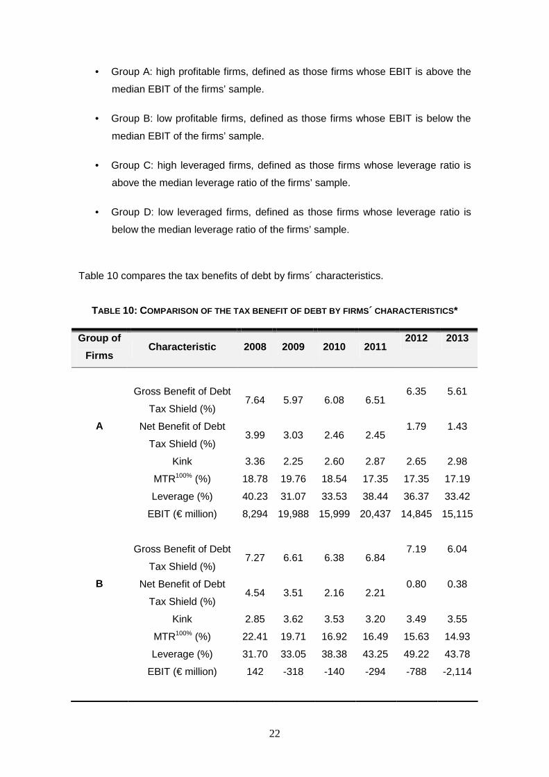
22

• Group A: high profitable firms, defined as those firms whose EBIT is above the

median EBIT of the firms’ sample.

• Group B: low profitable firms, defined as those firms whose EBIT is below the

median EBIT of the firms’ sample.

• Group C: high leveraged firms, defined as those firms whose leverage ratio is

above the median leverage ratio of the firms’ sample.

• Group D: low leveraged firms, defined as those firms whose leverage ratio is

below the median leverage ratio of the firms’ sample.

Table 10 compares the tax benefits of debt by firms´ characteristics.

TABLE 10: COMPARISON OF THE TAX BENEFIT OF DEBT BY FIRMS ´ CHARACTERISTICS*

Group of

Firms Characteristic 2008 2009 2010 2011

2012 2013

Gross Benefit of Debt

Tax Shield (%) 7.64 5.97 6.08 6.51

6.35 5.61

Net Benefit of Debt

Tax Shield (%) 3.99 3.03 2.46 2.45

1.79 1.43

Kink 3.36 2.25 2.60 2.87 2.65 2.98

MTR100% (%) 18.78 19.76 18.54 17.35 17.35 17.19

Leverage (%) 40.23 31.07 33.53 38.44 36.37 33.42

A

EBIT (€ million) 8,294 19,988 15,999 20,437 14,845 15,115

Gross Benefit of Debt

Tax Shield (%) 7.27 6.61 6.38 6.84

7.19 6.04

Net Benefit of Debt

Tax Shield (%) 4.54 3.51 2.16 2.21

0.80 0.38

Kink 2.85 3.62 3.53 3.20 3.49 3.55

MTR100% (%) 22.41 19.71 16.92 16.49 15.63 14.93

Leverage (%) 31.70 33.05 38.38 43.25 49.22 43.78

B

EBIT (€ million) 142 -318 -140 -294 -788 -2,114

23

Gross Benefit of Debt

Tax Shield (%) 11.57 10.12 9.75 10.29 10.32 8.85

Net Benefit of Debt

Tax Shield (%) 6.78 5.33 3.57 3.56 1.69 1.04

Kink 2.20 2.95 2.74 2.43 2.50 2.41

MTR100% (%) 21.71 19.84 17.24 16.45 15.43 15.17

Leverage (%) 54.43 51.01 56.57 63.17 67.11 60.81

C

EBIT (€ million) 4,209 15,083 10,592 15,176 4,325 4,862

Gross Benefit of Debt

Tax Shield (%) 3.33 2.46 2.79 3.06 3.31 2.88

Net Benefit of Debt

Tax Shield (%) 1.75 1.22 1.08 1.09 0.90 0.75

Kink 4.02 2.92 3.37 3.63 3.64 4.10

MTR100% (%) 19.48 19.63 18.23 17.39 17.51 16.90

Leverage (%) 17.50 13.11 15.76 18.52 19.18 17.03

D

EBIT (€ million) 4,227 4,586 5,266 4,966 9,731 8,138

*Both gross and net benefits of debt tax shield are computed in terms of firm´s market value. Leverage is the quotient between total book debt and firm´s market value.

Consistent with the findings of Blouin et al. (2010), we observe that kink increases with

profitability.

6. Robustness of results

In order to verify the robustness of our previous empirical evidence, we perform several

different tests.

A number of studies have attempted to analyze the tax implications of financing

decisions on the firm´s value by considering the interest expense instead of the debt

level as explanatory variable (see Fama and French 1998; Kemsley and Nissim, 2002;

Jayaraman, 2006; Sinha and Bansal, 2014, among others). Therefore, our first

robustness test will consist of including the interest expense variable in the regression

analysis. Following previous research, we formulate the following empirical

specification:

24

it it it it0 1 2 3

it it it it

it4 5 it

it

VALUE INT OI DIVβ β β β

Total Assets Total Assets Total Assets Total Assets

CAPEX β β SIZE ε

Total Assets

= + ⋅ + ⋅ + ⋅ +

+ ⋅ + ⋅ + [16]

Where VALUE is the difference between market and book value of the firm, INT is the

interest expense and constitutes the pivotal value (i.e., its coefficient leads to the

estimated value for the debt tax shield), OI is earnings before interest and taxes times

one minus marginal corporate tax rate, DIV is the amount of dividends paid, CAPEX is

capital expenditures, and SIZE is the natural logarithm of sales10.

Estimating Equation [16] requires to test for the potential endogeneity of the

contemporaneous interest variable. The implementation of Hausman (1978) test of

endogeneity results in the absence of endogeneity for the interest regressor11.

Table 11 shows the estimated coefficients of Equation [16].

TABLE 11: ESTIMATION RESULTS OF EQUATION [16]

Explanatory

Variables

Dependent Variable:

VALUE

INT

OI

DIV

CAPEX

SIZE

7.705* (1.93)

-0.757 (-1.44)

4.384*** (3.28)

-0.189 (-0.34)

0.016 (0.32)

Observations

432

10 Fama and French (1998) argue that poor controls for future profitability could distort the relation between firm value and debt. In order to cope with this concern, we include capital expenditures to better control for the firm´s future profitability, and firm´s size to take into account other firm level factors. 11 χ2=0.81 (0.999) accepting the null of absence of endogeneity.

25

R-Squared Within

Wald test (F-

statistic)

Hausman test (χ2)

0.1472

5.82 (0.000)

88.90 (0.000)

Fixed–effect regression coefficients estimated from Equation [16] with t-statistic in brackets. Superscript asterisks indicate statistical significance at 0.01(***), 0.05(**) and 0.10(*) levels. Wald’s test statistic refers to the null hypothesis that all coefficients of the explanatory variables are equal to zero. Hausman’s test refers to the null hypothesis of both fixed effects and random effects being equivalent.

The interpretation of the estimated coefficient associated to the interest variable (i.e.

β1) is the following. Recall that the value of a leveraged firm is the sum of the value of

the unleveraged firm and the present value of the debt tax shield. We can compute the

present value of the debt tax shield as the quotient between the marginal tax rate and

the capitalization rate (i.e. cost of debt) times the interest expense. Therefore, the

estimated marginal tax rate may be calculated as c 1 dˆt̂ β r= ⋅ . Specifically, 7.705

multiplied by the median interest rate (3.14%) equals 24.19%, which represents the

debt tax shield in terms of debt value. If we now multiply 24.19% by the mean leverage

ratio (39.81%), we obtain the debt tax shield in terms of firm value (9.63%).

Estimation of Equation [15] with interest expense instead of debt.

TABLE 12: ESTIMATION RESULTS OF EQUATION [15]

β0 β1 β2 β3 β4 Debt

Tax

Shield

γ2 γ3 γ4

Mean 0.7927 0.0075 0.0014 -

0.0471 0.0083 3.4696

-

3,641,031 50,173 202,167

t-

statistic 6.43 1.28 0.98 -6.47 2.55 1.74 -6.66 0.19 1.12

26

Nonlinear panel data regression coefficients estimated from Equation [15].

Multiplying the median interest rate (3.14%) by 3.4696 leads to the debt tax shield in

terms of debt value (10.89%). The debt tax shield in terms of firm value results from

multiplying 10.89% by the mean leverage ratio (39.81%) which mounts up to 4.34%.

7. Concluding remarks

Previous studies on debt tax shields have evaluated the determinants of debt usage or

the basic relationship between marginal tax rates and firms´ debt policy. On the

contrary, this study directly estimates the tax benefits of debt. It is the first empirical

analysis of the assessment of the tax benefit of debt, and how much it contributes to

firm value within Spanish context.

Our results prove that the tax benefits of debt for Spanish listed firms are significant.

Under the simulation approach, the mean capitalized gross tax benefit of current

interests is estimated to be 6.4% of firm value. For the entire sample period, the mean

incremental tax benefit is found to be 28.9% of firm value. Conversely, the regression

approach leads to a 11.2% (28.2%) debt tax shield in terms of firm (debt) value.

Robustness tests are in line with previous results.

The results of this study should provide insight into government regulations, especially

referred to tax code, on the capital structure of firms. Moreover, managers should be

aware of the relative importance of the value of debt tax benefits.

27

References

� Blouin, J., Core, J. E. and Guay, W., 2010, “Have the tax benefits of debt been

overestimated?”, Journal of Financial Economics, 98, 195-213. � Caskey, J., Hughes, J. and Liu, J., 2012, “Leverage, excess leverage, and future

returns”, Review of Accounting Studies, 17 (2), 443-471. � Clemente-Almendros, J. A. and Sogorb-Mira, F., 2015, “The effect of taxes on the

debt policy of Spanish listed companies”, Unpublished Working paper, University CEU Cardenal Herrera.

� Cooper, I. A. and Nyborg, K. G., 2006, “The value of tax shields is equal to the

present value of tax shields”, Journal of Financial Economics, 81, 215-225. � Cooper, I. A. and Nyborg, K. G., 2007, “Valuing the debt tax shield”, Journal of

Applied Corporate Finance, 19 (2), 50-59. � Doidge, D. and Dyck, A., 2015, “Taxes and corporate policies: Evidence from a

quasi natural experiment”, The Journal of Finance, 70 (1), 45-89. � Engel, E., Erickson, M. and Maydew, E., 1999, “Debt equity hybrid securities”,

Journal of Accounting Research, 37, 249–273. � Fama, E. F. and French, K. R., 1992, “The cross-section of expected stock returns”,

The Journal of Finance, 47 (2), 427-465. � Fama, E. F. and French, K. R., 1998, “Taxes, financing decisions, and firm value”,

The Journal of Finance, 53 (3), 819-843. � Gordon, R. and Mackie-Mason, J., 1990, “Effects of the Tax Reform Act 1986 on

corporate financial policy and organizational form” in J. Slemrod (Ed), Do taxes matter? The impact of the Tax Reform Act of 1986, MIT Press, Cambridge, MA.

� Graham, J. R., 1999, “Do personal taxes affect corporate financing decisions?”,

Journal of Public Economics, 73 (2), 147-185. � Graham, J. R., 2000, “How big are the tax benefits of debt?”, The Journal of

Finance, 55, 1901-1941. � Graham, J. R., 2001, “Estimating the tax benefits of debt”, Journal of Applied

Corporate Finance, 14 (1), 42-54. � Graham, J. R., 2003, “Taxes and corporate finance: A review”, Review of Financial

Studies, 16, 1075-1129. � Graham, J. R., 2008, “Taxes and corporate finance” in B. E. Eckbo (Ed), Handbook

of Corporate Finance. Empirical Corporate Finance, North-Holland Elsevier, Volume 2, Chapter 11, 59-133.

� Graham, J. R., 2013, “Do taxes affect corporate decisions? A Review” in G. M.

Constantinides, M. Harris and R. M. Stulz (Eds), Handbook of the Economics of Finance, North-Holland Elsevier, Volume 2, Part A, Chapter 3, 123-210.

28

� Graham, J. R., Lemmon, M. L. and Schallheim, J. S., 1998, “Debt, leases, taxes,

and the endogeneity of corporate tax status”, The Journal of Finance, 53 (1), 131-162.

� Green, R. C. and Hollifield, B., 2003, “The personal-tax advantages of equity”,

Journal of Financial Economics, 67 (2), 175-216. � Hanlon, M. and Heitzman, S., 2010, “A review of tax research”, Journal of

Accounting and Economics, 50, 127-178. � Hausman, J., 1978, “Specification tests in econometrics”, Econometrica, 46 (6),

1251-1271. � Hoaglin, D., 2003, “John W. Tukey and data analysis”, Statistical Science, 18 (3),

311-318. � Jayaraman, S., 2006, “Firm value and the tax benefit of debt”, Unpublished

Working paper, University of North Carolina. � Kaplan, S., 1989, “Management buyouts: evidence on taxes as a source of value”,

The Journal of Finance, 44 (3), 611-632. � Kemsley, D. and Nissim, D., 2002, “Valuation of the debt tax shield”, The Journal of

Finance, 57 (5), 2045-2073. � Ko, J. K. and Yoon, S., 2011, “Tax benefits of debt and debt financing in Korea”,

Asia-Pacific Journal of Financial Studies, 40, 824-855. � Korteweg, A., 2010, “The net benefits to leverage”, The Journal of Finance, 65,

2137-2170. � Masulis, R. W., 1983, “The impact of capital structure change on firm value: some

estimates”, Journal of Finance, 38, 107-126. � McGuire, S. T., Neuman, S. S., Olson, A. J. and Omer, T. C., 2014, “Valuation and

pricing of tax loss carryforwards”, Available at SSRN: http://dx.doi.org/10.2139/ssrn.2347635.

� Miller, M. H., 1977, “Debt and taxes”, The Journal of Finance, 32, 261-275. � Modigliani, F. and Miller, M. H., 1958, “The cost of capital, corporation finance, and

the theory of investment”, American Economic Review, 48, 261-297. � Modigliani, F. and Miller, M. H., 1963, “Corporate income taxes and the cost of

capital: A correction”, American Economic Review, 53, 433-443. � Modigliani, F. and Miller, M. H., 1966, “Some estimates of the cost of capital to the

electric utility industry, 1954-57”, American Economic Review, 56 (3), 333-391. � Penman, S. H., 1996, “The articulation of price-earnings ratios and market-to-book

ratios and the evaluation of growth”, Journal of Accounting Research, 34 (2), 235-259.

29

� Sarkar, S., 2014, “Valuation of tax loss carryforwards”, Review of Quantitative Finance and Accounting, 2014, 43 (4), 803-828.

� Sinha, P. and Bansal, V., 2014, “Interrelationship between taxes, capital structure

decisions and value of the firm: A panel data study on Indian manufacturing firms”, MPRA Paper No 58310, University Library of Munich, Germany.

� Van Binsbergen, J., Graham, J. and Yang, J., 2010, “The cost of debt”, The Journal

of Finance 65, 2089-2136.

30

� APPENDIX

TABLE A1 DEFINITION OF VARIABLES

Variables Definition

MTR0% Marginal tax rate estimated following Graham et al. (1998) approach, and assuming the firm has no interest deductions

MTR100% Marginal tax rate estimated following Graham et al. (1998) approach, and using the actual firm´s interest deductions

Kink Point at which the tax benefit function starts to slope downwards

ZeroBen Point at which the tax benefit function equals zero

VL Market value of the firm calculated as market value of equity plus book value of debt

OI Operating income calculated as earnings before interest and taxes times one minus marginal corporate tax rate

NOA Net operating assets calculated as total assets minus operating liabilities

OL Operating liabilities (i.e. all non-debt liabilities)

βU Unlevered beta

D Total financial debt