How Many People Do You Know?: EfficientlyEstimating Personal Network Size

Tyler H. MCCORMICK, Matthew J. SALGANIK, and Tian ZHENG

In this article we develop a method to estimate both individual social network size (i.e., degree) and the distribution of network sizes in apopulation by asking respondents how many people they know in specific subpopulations (e.g., people named Michael). Building on thescale-up method of Killworth et al. (1998b) and other previous attempts to estimate individual network size, we propose a latent non-randommixing model which resolves three known problems with previous approaches. As a byproduct, our method also provides estimates of therate of social mixing between population groups. We demonstrate the model using a sample of 1,370 adults originally collected by McCartyet al. (2001). Based on insights developed during the statistical modeling, we conclude by offering practical guidelines for the design offuture surveys to estimate social network size. Most importantly, we show that if the first names asked about are chosen properly, theestimates from the simple scale-up model enjoy the same bias-reduction as the estimates from our more complex latent nonrandom mixingmodel.

KEY WORDS: Latent nonrandom mixing model; Negative binomial distribution; Personal network size; Social networks; Survey design.

1. INTRODUCTION

Social networks have become an increasingly commonframework for understanding and explaining social phenom-ena. But despite an abundance of sophisticated models, socialnetwork research has yet to realize its full potential, in part be-cause of the difficulty of collecting social network data. In thisarticle we add to the toolkit of researchers interested in net-work phenomena by developing methodology to address twofundamental challenges posed in the seminal work of Pool andKochen (1978). First, for an individual, we would like to knowhow many other people she knows (i.e., her degree, di); and sec-ond, for a population, we would like to know the distribution ofacquaintance volume (i.e., the degree distribution, pd).

Recently, the second question, of degree distribution, has re-ceived the most attention because of interest in so-called “scale-free” networks (Barabási 2003). This interest was sparked bythe empirical finding that some networks, particularly techno-logical networks, appear to have power law degree distributions[i.e., p(d) ! d"! for some constant !], as well as by mathe-matical and computational studies demonstrating that this ex-tremely skewed degree distribution may affect the dynamics ofprocesses occurring on the network, such as the spread of dis-eases and the evolution of group behavior (Pastor-Satorras andVespignani 2001; Santos, Pacheco, and Lenaerts 2006). The de-gree distribution of the acquaintanceship network is not known,however, and this has become so central to some researchersthat Killworth et al. (2006) declared that estimating the degreedistribution is “one of the grails of social network theory.”

Tyler H. McCormick is Ph.D. Candidate, Department of Statistics, ColumbiaUniversity, New York, NY 10027 (E-mail: tyler@stat.columbia.edu). MatthewJ. Salganick is Assistant Professor, Department of Sociology and Office ofPopulation Research, Princeton University, Princeton, NJ 08544 (E-mail:mjs3@princeton.edu). Tian Zheng is Associate Professor, Department of Sta-tistics, Columbia University, New York, NY 10027 (E-mail: tzheng@stat.columbia.edu). This work was supported by National Science Foundation grantDMS-0532231 and a graduate research fellowship, and by the Institute forSocial and Economic Research and Policy and the Applied Statistics Cen-ter at Columbia University. The authors thank Peter Killworth, Russ Bernard,and Chris McCarty for sharing their survey data, as well as Andrew Gelman,Thomas DiPrete, Delia Baldassari, David Banks, an associate editor, and twoanonymous reviewers for their constructive comments. All of the authors con-tributed equally to this work.

Although estimating the degree distribution is certainly im-portant, we suspect that the ability to quickly estimate the per-sonal network size of an individual may be of greater impor-tance to social science. Currently, the dominant framework forempirical social science is the sample survey, which has beenastutely described by Barton (1968) as a “meat grinder” thatcompletely removes people from their social contexts. Having asurvey instrument that allows for the collection of social contentwould allow researchers to address a wide range of questions.For example, to understand differences in status attainment be-tween siblings, Conley (2004) wanted to know whether siblingswho knew more people tended to be more successful. Becauseof difficulty in measuring personal network size, his analysiswas ultimately inconclusive.

In this article we report a method developed to estimate bothindividual network size and degree distribution in a popula-tion using a battery of questions that can be easily embeddedinto existing surveys. We begin with a review of previous at-tempts to measure personal network size, focusing on the scale-up method of Killworth et al. (1998b), which is promising butis known to suffer from three shortcomings: transmission er-rors, barrier effects, and recall error. In Section 3 we propose alatent nonrandom mixing model that resolves these problems,and as a byproduct allows for the estimation of social mixingpatterns in the acquaintanceship network. We then fit the modelto 1,370 survey responses from McCarty et al. (2001), a nation-ally representative telephone sample of Americans. In Section 5we draw on insights developed during the statistical modelingto offer practical guidelines for the design of future surveys.

2. PREVIOUS RESEARCH

The most straightforward method for estimating the personalnetwork size of respondents would be to simply ask them howmany people they “know.” We suspect that this would workpoorly, however, because of the well-documented problemswith self-reported social network data (Killworth and Bernard1976; Bernard et al. 1984; Brewer 2000; Butts 2003). Other,

© 2010 American Statistical AssociationJournal of the American Statistical Association

March 2010, Vol. 105, No. 489, Applications and Case StudiesDOI: 10.1198/jasa.2009.ap08518

59

60 Journal of the American Statistical Association, March 2010

more clever attempts have been made to measure personal net-work size, including the reverse small-world method (Killworthand Bernard 1978; Killworth, Bernard, and McCarty 1984;Bernard et al. 1990), the summation method (McCarty et al.2001), the diary method (Gurevich 1961; Pool and Kochen1978; Fu 2007; Mossong et al. 2008), the phonebook method(Pool and Kochen 1978; Freeman and Thompson 1989; Kill-worth et al. 1990), and the scale-up method (Killworth et al.1998b).

We believe that the scale-up method has the greatest poten-tial for providing accurate estimates quickly with reasonablemeasures of uncertainty. But the scale-up method is known tosuffer from three distinct problems: barrier effects, transmis-sion effects, and recall error (Killworth et al. 2003, 2006). InSection 2.1 we describe the scale-up method and these threeissues in detail, and in Section 2.2 we present an earlier modelby Zheng, Salganik, and Gelman (2006) that partially addressessome of these issues.

2.1 The Scale-Up Method and Three Problems

Consider a population of size N. We can store the informa-tion about the social network connecting the population in anadjacency matrix, ! = ["ij]N#N , such that "ij = 1 if person iknows person j. Although our method does not depend on thedefinition of “know,” throughout we assume McCarty et al.(2001)’s definition: “that you know them and they know youby sight or by name, that you could contact them, that they livewithin the United States, and that there has been some contact(either in person, by telephone or mail) in the past 2 years.” Thepersonal network size or degree of person i is then di = !

j "ij.One straightforward way to estimate the degree of person i

would be to ask if she knows each of n randomly chosen mem-bers of the population. Inference then could be based on the factthat the responses would follow a binomial distribution with ntrials and probability di/N. This method is extremely inefficientin large populations, however, because the probability of a rela-tionship between any two people is very low. For example, as-suming an average personal network size of 750 (as estimatedby Zheng, Salganik, and Gelman 2006), the probability of tworandomly chosen Americans knowing each other is only about0.0000025, meaning that a respondent would need to be askedabout millions of people to produce a decent estimate.

A more efficient method would be to ask the respondentabout an entire set of people at once, for example, asking“how many women do you know who gave birth in the last12 months?” instead of asking if she knows 3.6 million distinctpeople. The scale-up method uses responses to questions of thisform (“How many X’s do you know?”) to estimate personalnetwork size. For example, if a respondent reports knowing 3women who gave birth, this represents about 1-millionth of allwomen who gave birth within the last year. This informationthen could be used to estimate that the respondent knows about1-millionth of all Americans,

33.6 million

· (300 million) $ 250 people. (1)

The precision of this estimate can be increased by averaging re-sponses of many groups, yielding the scale-up estimator (Kill-worth et al. 1998b)

d̂i =!K

k=1 yik!Kk=1 Nk

· N, (2)

where yik is the number of people that person i knows in sub-population k, Nk is the size of subpopulation k, and N is thesize of the population. One important complication to note withthis estimator is that asking “how many women do you knowwho gave birth in the last 12 months?” is equivalent not to ask-ing about 3.6 million random people, but rather to asking aboutwomen roughly age 18–45. This creates statistical challengesthat we address in detail in later sections.

To estimate the standard error of the simple estimate, we fol-low the practice of Killworth et al. (1998a) by assuming

K"

k=1

yik ! Binomial

#K"

k=1

Nk,di

N

$

. (3)

The estimate of the probability of success, p = di/N, is

p̂ =!k

i=1 yik!Kk=1 Nk

= d̂i

N, (4)

with standard error (including finite population correction)(Lohr 1999)

SE(p̂) =

%&&' 1!K

k=1 Nkp̂(1 " p̂)

N " !Kk=1 Nk

N " 1.

The scale-up estimate d̂i then has standard error

SE(d̂i) = N · SE(p̂)

= N

%&&' 1!K

k=1 Nkp̂(1 " p̂)

N " !Kk=1 Nk

N " 1

$

%&&'N " !Kk=1 Nk!K

k=1 Nkd̂i =

(d̂i ·

%&&'1 " !Kk=1 Nk/N

!Kk=1 Nk/N

. (5)

For example, when asking respondents about the number ofwomen they know who gave birth in the past year, the approxi-mate standard error of the degree estimate is calculated as

SE(d̂i) $(

d̂i ·

%&&'1 " !Kk=1 Nk/N

!Kk=1 Nk/N

$%

750 ·)

1 " 3.6 million/300 million3.6 million/300 million

$ 250,

assuming a degree of 750 as estimated by Zheng, Salganik, andGelman (2006).

If we also had asked respondents about the number of peo-ple they know who have a twin sibling, the number of peoplethey know who are diabetics, and the number of people theyknow who are named Michael, we would have increased ouraggregate subpopulation size,

!Kk=1 Nk, from 3.6 million to ap-

proximately 18.6 million, and in doing so decreased our esti-

mated standard error to about 100. Figure 1 plots SE(d̂i)/

(d̂i

against!k

k=1 Nk/N. The most drastic reduction in estimatederror comes in increasing the survey fractional subpopulationsize to about 20% (or approximately 60 million in a popu-lation of 300 million). Although the foregoing standard errordepends only on the sum of the subpopulation sizes, there are

McCormick, Salganik, and Zheng: Estimating Personal Network Size 61

Figure 1. Standard error of the scale-up degree estimate (scaled bythe square root of the true degree) plotted against the sum of the frac-tional subpopulation sizes. As the fraction of population representedby survey subpopulations increases, the precision of the estimate im-proves. Improvements diminish after about 20%.

other sources of bias that make the choice of the individual sub-populations important, as we show later.

The scale-up estimator using “how many X do you know?”data is known to suffer from three distinct problems: transmis-sion errors, barrier effects, and recall problems (Killworth et al.2003, 2006). Transmission errors occur when the respondentknows someone in a specific subpopulation but is not awarethat the person is actually in that subpopulation; for example,a respondent might know a woman who recently gave birth butmight not know that the woman had recently given birth. Thesetransmission errors likely vary from subpopulation to subpop-ulation depending on the sensitivity and visibility of the infor-mation. These errors are extremely difficult to quantify, becausevery little is known about how much information respondentshave about the people they know (Laumann 1969; Killworthet al. 2006; Shelley et al. 2006).

Barrier effects occur whenever some individuals systemati-cally know more (or fewer) members of a specific subpopula-tion than would be expected under random mixing, and thusalso can be called nonrandom mixing. For example, becausepeople tend to know others of similar age and gender (McPher-son, Smith-Lovin, and Cook 2001), a 30-year old woman prob-ably knows more women who have recently given birth thanwould be predicted based solely on her personal network sizeand the number of women who have recently given birth. Sim-ilarly, an 80-year-old man probably knows fewer such womenthan would be expected under random mixing. Consequently,estimating personal network size by asking only “how manywomen do you know who have recently given birth?”—the es-timator presented eq. (1)—will tend to overestimate the degreeof women in their 30s and underestimate the degree of men intheir 80s. Because these barrier effects can introduce a bias ofunknown size, they have prevented previous researchers fromusing the scale-up method to estimate the degree of any partic-ular individual.

A final source of error is that responses to these questionsare prone to recall error. For example, people seem to under-recall the number of people they know in large subpopulations

(e.g., people named Michael) and overrecall the number of peo-ple they in small subpopulations (e.g., people who committedsuicide) (Killworth et al. 2003; Zheng, Salganik, and Gelman2006).

2.2 The Zheng, Salganik, and Gelman (2006) ModelWith Overdispersion

Before presenting our model for estimating personal networksize using “how many X’s do you know?” data, it is importantto review the multilevel overdispersed Poisson model of Zheng,Salganik, and Gelman (2006), which, rather than treating non-random mixing (i.e., barrier effects) as an impediment to net-work size estimation, treats it as something important to esti-mate for its own sake. Zheng, Salganik, and Gelman (2006) be-gan by noting that under simple random mixing, the responsesto the “how many X’s do you know?” questions, yik’s, wouldfollow a Poisson distribution with rate parameter determined bythe degree of person i, di, and the network prevalence of groupk, bk. Here bk is the proportion of ties that involve individuals insubpopulation k in the entire social network. If we can assumethat individuals in the group being asked about (e.g., peoplenamed Michael) are as popular as the rest of the population onaverage, then bk $ Nk/N.

The responses to many of the questions in the data ofMcCarty et al. (2001) do not follow a Poisson distribution, how-ever. In fact, most of the responses show overdispersion, that is,excess variance given the mean. Consider, for example, the re-sponses to the question: “How many males do you know incar-cerated in state or federal prison?” The mean of the responses tothis question was 1.0, but the variance was 8.0, indicating thatsome people are much more likely than others to know some-one in prison. To model this increased variance, Zheng, Sal-ganik, and Gelman (2006) allowed individuals to vary in theirpropensity to form ties to different groups. If these propensitiesfollow a gamma distribution with a mean value of 1 and a shapeparameter of 1/(#k " 1), then the yik’s can be modeled with anegative binomial distribution,

yik ! Neg-Binom(mean = µik, overdispersion = #k), (6)

where µik = dibk. Thus #k estimates the variation in individualpropensities to form ties to people in different groups and rep-resents one way of quantifying nonrandom mixing (i.e., barriereffects).

Although it was developed to estimate #k, the model ofZheng et al. also produces personal network size estimates, di.These estimates are problematic for two reasons, however. First,the normalization procedure used to address recall problems(see Zheng, Salganik, and Gelman 2006 for complete details)only shifts the degree distribution back to the appropriate scale;it does not ensure that the degree of individual respondents arebeing estimated accurately. Second, the degree estimates fromthe model remain susceptible to bias due to transmission errorand barrier effects.

3. A NEW STATISTICAL METHOD FORDEGREE ESTIMATION

We now describe a new statistical procedure to address thethree aforementioned problems with estimating individual de-gree using “how many X’s do you know?” data. Transmission

62 Journal of the American Statistical Association, March 2010

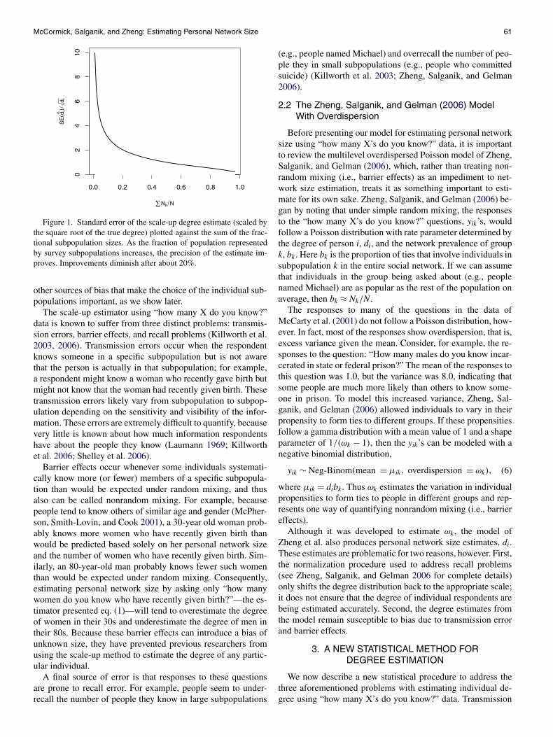
errors, while probably the most difficult to quantify, are also theeasiest to eliminate. We limit our analysis to the 12 subpopula-tions defined by first names that were asked about by McCartyet al. (2001). These 12 names (half male and half female) arepresented in Figure 2. Although McCarty et al.’s definition of“knowing” someone does not explicitly require respondents toknow individuals by name, we believe that using first namesprovides the minimum imaginable bias due to transmission er-rors; that is, it is unlikely that a person knows someone butdoes not know his or her first name. Even though using onlyfirst names controls transmission errors, it does not address biasfrom barrier effects or recall bias. In this section we propose alatent nonrandom mixing model to address these two issues.

3.1 Latent Nonrandom Mixing Model

We begin by considering the impact of barrier effects, or non-random mixing, on degree estimation. Imagine, for example, ahypothetical 30-year-old male survey respondent. If we were toignore nonrandom mixing and ask this respondent how manyMichaels he knows, then we would overestimate his networksize using the scale-up method, because Michael tends to be amore popular name among younger males (Figure 2). In con-trast, if we were to ask how many Roses he knows, then wewould underestimate the size of his network, because Rose isa name that is more common in older females. In both cases,the properties of the estimates are affected by the demographicprofiles of the names used, something not accounted for in thescale-up method.

We account for nonrandom mixing using a negative binomialmodel that explicitly estimates the propensity for a respondentin ego group e to know members of alter group a. Here we

are following standard network terminology (Wasserman andFaust 1994), referring to the respondent as ego and the peopleto whom he can form ties as alters. The model is then

yik ! Neg-Binom(µike,#&k),

where µike = di

A"

a=1

m(e,a)Nak

Na, (7)

where di is the degree of person i, e is the ego group to whichperson i belongs, Nak/Na is the relative size of name k withinalter group a (e.g., 4% of males age 21–40 are named Michael),and m(e,a) is the mixing coefficient between ego group e andalter group a, that is,

m(e,a) = E*

dia

di = !Aa=1 dia

+++i in ego group e,

, (8)

where dia is the number of person i’s acquaintances in altergroup a. That is, m(e,a) represents the expected fraction of theties of someone in ego group e that go to people in alter groupa. For any group e,

!Aa=1 m(e,a) = 1.

Thus the number of people that person i knows with namek, given that person i is in ego group e, is based on person i’sdegree (di), the proportion of people in alter group a that havename k (Nak/Na), and the mixing rate between people in groupe and people in group a [m(e,a)]. In addition, if we do notobserve nonrandom mixing, then m(e,a) = Na/N and µike in(7) reduces to dibk in (6).

Along with µike, the latent nonrandom mixing model also de-pends on the overdispersion, #&

k, which represents the variation

Figure 2. Age profiles for the 12 names used in the analysis (data source: SSA). The heights of the bars represent the percentage of Americannewborns in a given decade with a particular name. The total subpopulation size is given across the top of each graph. These age profiles arerequired to construct the matrix of Nak

Naterms in eq. (7). The male names chosen by McCarty et al. are much more popular than the female names.

McCormick, Salganik, and Zheng: Estimating Personal Network Size 63

in the relative propensity of respondents within an ego groupto form ties with individuals in a particular subpopulation k.Using m(e,a), we model the variability in relative propensitiesthat can be explained by nonrandom mixing between the de-fined alter and ego groups. Explicitly modeling this variationshould cause a reduction in overdispersion parameter #&

k com-pared with #k in (6) and Zheng, Salganik, and Gelman (2006).The term #&

k is still in the latent nonrandom mixing model, how-ever, because there remains residual overdispersion based onadditional ego and alter characteristics that could affect theirpropensity to form ties.

Fitting the model requires choosing the number of egogroups, E, and alter groups, A. In this case we classified egosinto six categories by crossing gender (2 categories) with threeage categories: youth (age 18–24 years), adult (age 25–64), andsenior (age 65+). We constructed eight alter groups by cross-ing gender with four age categories: 0–20, 21–40, 41–60, and61+. Thus to estimate the model, we needed to know the ageand gender of our respondents and, somewhat more problemat-ically, the the relative popularity of the name-based subpopula-tions in each alter group ( Nak

Na). We approximated this popularity

using the decade-by-decade birth records made available by theSocial Security Administration (SSA). Because we are usingthe SSA birth data as a proxy for the living population, we areassuming that several social processes—immigration, emigra-tion, and life expectancy—are uncorrelated with an individual’sfirst name. We also are assuming that the SSA data are accu-rate, even for births from the early twentieth century, when reg-istration was less complete. We believe that these assumptionsare reasonable as a first approximation and probably did nothave a substantial effect on our results. Together these model-ing choices resulted in a total of 48 mixing parameters, m(e,a),to estimate (6 ego groups by 8 alter groups). We believe thatthis represents a reasonable compromise between parsimonyand richness.

3.2 Correction for Recall Error

The model in eq. (7) is a model for the actual network ofthe respondents assuming only random sampling error. Unfor-tunately, however, the observed data rarely yield reliable in-formation about this network, because of the systematic ten-dency for respondents to underrecall the number of individualsthat they know in large subpopulations (Killworth et al. 2003;Zheng, Salganik, and Gelman 2006). For example, assume thata respondent recalls knowing five people named Michael; thenthe estimated network size would be

54.8 million/300 million

$ 300 people. (9)

But Michael is a common name, making it likely that thereare additional Michaels in the respondent’s actual network whowere not counted at the time of the survey (Killworth et al.2003; Zheng, Salganik, and Gelman 2006). We could chooseto address this issue in two ways, which, although ultimatelyequivalent, suggest two distinct modeling strategies.

First, we could assume that the respondent is inaccurately re-calling the number of people named Michael that she knowsfrom her true network. Under this framework, any correctionthat we propose should increase the numerator in eq. (9). This

requires that we propose a mechanism by which respondentsunderreport their true number known on individual questions.In our example, this would be equivalent to taking the fiveMichaels reported and applying some function to produce a cor-rected response (presumably some number greater than five),which then would be used to fit the proposed model. It is diffi-cult to speculate about the nature of this function in any detail,however.

Another approach would be to assume that respondents arerecalling not from their actual network, but rather from a re-called network that is a subset of the actual network. We spec-ulate that the recalled network is created when respondentschange their definition of “know” based on the fraction of theirnetwork made up of the population being queried such that theyuse a more restrictive definition of “know” when answeringabout common subpopulations (e.g., people named Michael)than when answering about rare subpopulations (e.g., peoplenamed Ulysses). This means that, in the context of Section 2.2,we no longer have that bk $ Nk/N. We can, however, usethis information for calibration, because the true subpopulationsizes, Nk/N, are known and can be used as a point of compari-son to estimate and then correct for the amount of recall bias.

Previous empirical work (Killworth et al. 2003; Zheng, Sal-ganik, and Gelman 2006; McCormick and Zheng 2007) sug-gests that the calibration curve, f (·), should impose less cor-rection for smaller subpopulations and progressively greatercorrection as the popularity of the subpopulation increases.Specifically, both Killworth et al. (2003) and Zheng, Salganik,and Gelman (2006) suggested that the relationship between$k = log(bk) and $ &

k = log(b&k) begins along the y = x line, and

that the slope decreases to 1/2 (corresponding to a square rootrelation on the original scale) with increasing fractional sub-population size.

Using these assumptions and some boundary conditions,McCormick and Zheng (2007) derived a calibration curve thatgives the following relationship between bk and b&

k:

b&k = bk

-c1

bkexp

*1c2

*1 "

.c1

bk

/c2,,01/2

, (10)

where 0 < c1 < 1 and c2 > 0. By fitting the curve to the namesfrom the McCarty et al. (2001) survey, we chose c1 = e"7 andc2 = 1. (For details on this derivation, see McCormick andZheng 2007.) We apply the curve to our model as follows:

yik ! Neg-Binom(µike,#&k),

where µike = dif

#A"

a=1

m(e,a)Nak

Na

$

. (11)

3.3 Model Fitting Algorithm

Here we use a multilevel model and Bayesian inference toestimate di, m(e,a), and #&

k in the latent nonrandom mixingmodel described in Section 3.1. We assume that log(di) fol-

64 Journal of the American Statistical Association, March 2010

lows a normal distribution with mean µd and standard devia-tion %d . Zheng, Salganik, and Gelman (2006) postulated thatthis prior should be reasonable based on previous work, specif-ically McCarty et al. (2001), and found that the prior workedwell in their case. We estimate a value of m(e,a) for all E egogroups and all A alter groups. For each ego group, e, and eachalter group, a, we assume that m(e,a) has a normal prior distrib-ution with mean µm(e,a) and standard deviation %m(e,a). For #&

k,we use independent uniform(0,1) priors on the inverse scale,p(1/#&

k) ' 1. Because #&k is constrained to (1,(), the inverse

falls on (0,1). The Jacobian for the transformation is #&"2k . Fi-

nally, we give noninformative uniform priors to the hyperpa-rameters µd , µm(e,a), %d , and %m(e,a). Then the joint posteriordensity can be expressed as

p1d,m(e,a),#&,µd,µm(e,a),%d,%m(e,a)|y

2

'K3

k=1

N3

i=1

*yik + &ik " 1

&ik " 1

,*1#&

k

,&ik*

#&k " 1#&

k

,yik

#N3

i=1

*1#&

k

,2

N(log(di)|µd,%d)

#E3

e=1

N1m(e,a)|µm(e,a),%m(e,a)

2, (12)

where &ik = dif (!A

a=1 m(e,a)NakNa

)/(#&k " 1).

Adapting Zheng, Salganik, and Gelman (2006), we use aGibbs–Metropolis algorithm in each iteration v, as follows:

1. For each i, update di using a Metropolis step with jumpingdistribution log(d)

i ) ! N(d(v"1)i , (jumping scale of di)

2).2. For each e, update the vector m(e, ·) using a Metropo-

lis step. Define the proposed value using a random di-rection and jumping rate. Each of the A elements ofm(e, ·) has a marginal jumping distribution m(e,a)) !N(m(e,a)(v"1), (jumping scale of m(e, ·))2). Then rescaleso that the row sum is 1.

3. Update µd ! N(µ̂d,%2d /n), where µ̂d = 1

n

!ni=1 di.

4. Update % 2d ! Inv-'2(n"1, %̂ 2

d ), where %̂ 2d = 1

n

!ni=1(di "

µd)2.

5. Update µm(e,a) ! N(µ̂m(e,a),%2m(e,a)/A) for each e where

µ̂m(e,a) = 1A

!Aa=1 m(e,a).

6. Update % 2m(e,a) ! Inv-'2(A " 1, %̂ 2

m(e,a)) for each e, where

%̂ 2m(e,a) = 1

A

!Aa=1(m(e,a) " µm(e,a))

2.7. For each k, update #&

k using a Metropolis step with jump-ing distribution #&)

k ! N(#&(v"1)k , (jumping scale of #&

k)2).

4. RESULTS

To fit the model, we used data from McCarty et al. (2001),comprising survey responses from 1,370 adults living in theUnited States who were contacted via random digit dialing intwo surveys: survey 1, with 796 respondents, conducted in Jan-uary 1998, and survey 2, with 574 respondents, conducted inJanuary 1999. To correct for responses that were suspiciouslylarge (e.g., a person claiming to know more than 50 Michaels),we truncated all responses at 30, a procedure that affected only0.25% of the data. We also inspected the data using scatterplots,

which revealed a respondent who was coded as knowing sevenpeople in each subpopulation. We removed this case from thedata set.

We obtained approximate convergence of our algorithm(R̂max < 1.1; see Gelman et al. 2003) using three parallel chainswith 2,000 iterations per chain. We used the first half of eachchain for burn-in and thinned the chain by using every tenthiterate. All computations were performed using custom codewritten for the software package R (R Development Core Team2009), which is available on request.

4.1 Personal Network Size Estimates

We estimated a mean network size of 611 (median, 472). Fig-ure 3 presents the distribution of network sizes. In the figure,the solid line represents a log-normal distribution with para-meters determined via maximum likelihood (µ̂mle = 6.2 and%̂mle = 0.68); the lognormal distribution fits the distributionquite well. This result is not an artifact of our model, as has beenconfirmed by additional simulation studies (data not shown).Given the recent interest in power laws and networks, we alsoexplored the fit of the power law distribution (dashed line) withparameters estimated via maximum likelihood (!mle = 1.28)

(Clauset, Shalizi, and Newman 2007). The fit is clearly poor, aresult consistent with previous work showing that another socialnetwork—the sexual contact network—also is poorly approxi-mated by the power law distribution (Hamilton, Handcock, andMorris 2008).

Figure 4 compares the estimated degree from the latentnonrandom mixing model with estimates obtained using themethod of Zheng, Salganik, and Gelman (2006). In general, the

Figure 3. Estimated degree distribution from the fitted model. Themedian is about 470, and the mean is about 610. The shading repre-sents random draws from the posterior distribution to indicate inferen-tial uncertainty in the histograms. The solid line is a log-normal distri-bution fit using maximum likelihood to the posterior median for eachrespondent (µ̂mle = 6.2 and %̂mle = 0.68). The dashed line is a powerlaw density with scaling parameter estimated by maximum likelihood(!̂mle = 1.28).

McCormick, Salganik, and Zheng: Estimating Personal Network Size 65

Figure 4. Comparison of the estimates from Zheng et al. and the latent nonrandom mixing model broken down by age and gender. Graypoints represent males; black points, females. The latent nonrandom mixing model accounts for the fact that the names from McCarty et al. arepredominately male and predominantly middle-aged, and thus produces lower degree estimates for respondents in these groups. Because ourmodel has six ego groups, there are six distinct patterns in the figure.

estimates from the latent nonrandom mixing model tend to beslightly smaller, with an estimated median degree of 472 (mean,611), compared with that of 610 (mean 750) obtained using themethod of Zheng, Salganik, and Gelman (2006). Figure 4 alsoreveals that the differences between the estimates vary in waysthat are expected given that the names in the data of McCarty etal. are predominantly male and predominantly middle-aged (seeFigure 2). The latent nonrandom mixing model accounts for thisfact, and thus produces lower estimates for male respondentsand adult respondents than the method of Zheng, Salganik, andGelman (2006).

4.2 Mixing Estimates

Although our proposed procedure was developed to obtaingood estimates of personal network size, it also provides in-formation about the mixing rates in the population, which isconsidered to affect the spread of information (Volz 2006) anddisease (Morris 1993; Mossong et al. 2008). Even though previ-ous work has been done on estimating population mixing rates

(see, e.g., Morris 1991), we believe this is the first survey-basedapproach for estimating such information indirectly.

As mentioned in the previous section, the mixing matrix,m(e,a), represents the proportion of the network of a person inego group e that is composed of people in alter group a. The es-timated mixing matrix presented in Figure 5 indicates plausiblerelationships within subgroups, with the dominant pattern be-ing that individuals tend to preferentially associate with othersof similar age and gender, a finding consistent with the largesociological literature on homophily (the tendency for peopleto form ties to those who are similar to themselves) (McPher-son, Smith-Lovin, and Cook 2001). This trend is especially ap-parent in adult males, who demonstrate a high proportion oftheir ties to other males. With additional information on therace/ethinicity of the different names, the latent nonrandommixing model could be used to estimate the extent of socialnetwork–based segregation, an approach that could have manyadvantages over traditional measures of residential segregation(Echenique and Fryer 2007).

Figure 5. Barplot of the mixing matrix. Each of the six stacks of bars represents one ego group. Each stack describes the proportion of thegiven ego group’s ties that are formed with all of the alter groups; thus the total proportion within each stack is 1. For each individual bar, a shiftto the left indicates an increased propensity to know female alters. Thick lines represent ±1 standard error (estimated from the posterior); thinlines, ±2 standard errors.

66 Journal of the American Statistical Association, March 2010

4.3 Overdispersion

Another way to assess the latent nonrandom mixing model isto examine the overdispersion parameter #&

k, which representsthe variation in propensity to know individuals in a particulargroup. In the latent nonrandom mixing model, a portion of thisvariability is modeled by the ego group–dependent mean, µike.The remaining unexplained variability forms the overdisper-sion parameter, #&

k. In Section 3.1 we predicted that #&k would

be smaller than the overdispersion #k reported by Zheng, Sal-ganik, and Gelman (2006), because Zheng, Salganik, and Gel-man (2006) did not model nonrandom mixing.

This prediction turned out to be correct. With the excep-tion of Anthony, all of the estimated overdispersion estimatesfrom the latent nonrandom mixing model are lower than thosepresented by Zheng, Salganik, and Gelman (2006). To judgethe magnitude of the difference, we created a standardized dif-

ference measure,#&

k"#k#k"1 . Here the numerator, #&

k " #k, repre-sents the reduction in overdispersion resulting from modelingnonrandom mixing explicitly in the latent nonrandom mixingmodel. In the denominator, an #k value of 1 corresponds tono overdispersion; thus the ratio for group k is the proportionof overdispersion encountered in Zheng, Salganik, and Gelman(2006) that is explicitly modeled in the latent nonrandom mix-ing model. The standardized difference was on average 0.213units lower for the latent nonrandom mixing model estimates,indicating that roughly 21% of the overdispersion found inZheng, Salganik, and Gelman (2006) can be explained by non-random mixing due to age and gender. If appropriate ethnicityor other demographic information about the names were avail-able, then we would expect this reduction to be even larger.

5. DESIGNING FUTURE SURVEYS

In the preceding sections we analyzed existing data in sucha way as to resolve the three known problems with estimat-ing personal network size from “how many X’s do you know?”data. In this section we offer survey design suggestions that canallow researchers to capitalize on the simplicity of the scale-upestimates while enjoying the same bias reduction as in the la-tent nonrandom mixing model. Thus this section provides anefficient and easily applied degree estimation method that is ac-cessible to a wide range of researchers who may not wish to fitthe latent nonrandom mixing model.

In Section 5.1 we derive the requirement for selecting firstnames such that the scale-up estimate is equivalent to the de-gree estimate derived from fitting a latent nonrandom mixingmodel using Markov chain Monte Carlo computation. The in-tuition behind this result is that the names asked about shouldbe chosen so that the combined set of people asked about is a“scaled-down” version of the overall population; for example,if 20% of the general population is females under age 30, then20% of the people with the names used also must be femalesunder age 30. Section 5.2 presents practical advice for choos-ing such a set of names and presents a simulation study of theperformance of the suggested guidelines. Finally, Section 5.3offers guidelines on the standard errors of the estimates.

5.1 Selecting Names for the Scale-Up Estimator

Unlike the scale-up estimator (2), the latent nonrandom mix-ing model accounts for barrier effects due to some demographicfactors by estimating degree differentially based on character-istics of the respondent and of the potential alter population.But if there were conditions under which the simple scale-upestimator was expected to be equivalent to the latent nonran-dom mixing model, then the simple estimator would enjoy thesame reduction of bias from barrier effects as the more com-plex latent nonrandom mixing model estimator. In this sectionwe derive such conditions.

The latent nonrandom mixing model assumes an expectednumber of acquaintances for an individual i in ego group e topeople in group k [as in (7)],

µike = E(yike) = di

A"

a=1

m(e,a)Nak

Na.

In contrast, the scale-up estimator assumes that

E

#K"

k=1

yike

$

=K"

k=1

µike = di

A"

a=1

m(e,a)

-K"

k=1

Nak

Na

0

* di

!Kk=1

!Aa=1 Nak

N, +e. (13)

Equation (13) shows that the scale-up estimator of Killworth etal. (2) is in expectation equivalent to that of the latent nonran-dom mixing if either

m(e,a) = Na

N, +a,+e (14)

or!K

k=1 Nak!Kk=1 Nk

= Na

N, +a. (15)

In other words, the two estimators are equivalent if there is ran-dom mixing (14) or if the combined set of names representsa “scaled-down” version of the population (15). Because ran-dom mixing is not a reasonable assumption for the acquain-tances network in the United States, we need to focus on se-lecting the names to satisfy the scaled-down condition; that is,we should select the set of names such that if 15% of the pop-ulation is males between age 21 and 40 ( Na

N ), then 15% of thepeople asked about also must be males between age 21 and 40

(!K

k=1 Nak!Kk=1 Nk

).

When actually choosing a set of names to satisfy the scaled-down condition, we found it more convenient to work with arearranged form of (15),

!Kk=1 Nak

Na=

!Kk=1 Nk

N, +a. (16)

To find a set of names that satisfy (16), it is helpful to cre-ate Figure 6, which displays the relative popularity of manynames over time. From this figure, we tried to select a set ofnames such that the popularity across alter categories ended upbalanced. Consider, for example, the names Walter, Bruce, andKyle. These names have similar popularity overall, but Walterwas popular in 1910–1940, whereas Bruce was popular during

McCormick, Salganik, and Zheng: Estimating Personal Network Size 67

Figure 6. Heat maps of additional male and female names based on SSA data. Lighter color indicates higher popularity.

the middle of the twentieth century, and Kyle was popular nearthe end of the century. Thus the popularity of the names dur-ing any one time period will be balanced by the popularity ofother names in the other time periods, preserving the requiredequality in the sum (16).

When choosing what names to use, besides satisfyingeq. (16), we recommend choosing names that compromise0.1%–0.2% of the population, which will minimize recall errorsand yield average responses of 0.6–1.3. Finally, we recommendchoosing names not commonly associated with nicknames, tominimize transmission errors.

5.2 Simulation Study

We now demonstrate the use of the foregoing guidelines in asimulation study. Again we use the age and gender profiles ofthe names as an example. If other information were available,then the general approach presented here would still be applica-ble.

Figure 6 shows the popularity profiles of several names withthe desired level of overall popularity (0.1%–0.2% of the popu-lation). We used this figure to select two sets of names (Table 1).We selected the first set—the good names—using the proce-dure described in the previous section to satisfy the scaled-down condition. We also selected a second set of names—thebad names—that were popular with individuals born in the firstdecades of the twentieth century and thus did not satisfy thescaled-down condition. For comparison, we also use the set of12 names from the data of McCarty et al.

Table 1. A set of names that approximately meet the scaled-downcondition (the good names) and a set of names that do not

(the bad names)

Good names Bad names

Male Female Male Female

Walter Rose Walter AliceBruce Tina Jack MarieKyle Emily Harold RoseRalph Martha Ralph JoyceAlan Paula Roy MarilynAdam Rachel Carl Gloria

Figure 7 provides a visual check of the scaled-down con-dition (14) for these three sets of names by plotting the com-bined demographic profiles for each set compared with that ofthe overall population. The figure reveals clear problems withthe McCarty et al. names and the bad names. For example, inthe bad names, older individuals represent a much larger frac-tion of the subpopulation of alters compared with the overallpopulation (as expected given our method of selection). Thuswe would expect scale-up estimates based on the bad names tooverestimate the degree of older respondents.

We evaluated this prediction using a simulation study inwhich we fit the latent nonrandom mixing model to theMcCarty et al. data and then used these estimated parameters(i.e., degree, overdispersion, and mixing matrix) to generate anegative binomial sample of size 1,370. We then fit the scale-upestimate, the latent nonrandom mixing model, and the model ofZheng et al. to these simulated data to see how these estimatescould recover the known data-generating parameters.

Figure 8 presents the results of the simulation study. Ineach panel the difference between the estimated degree and theknown data-generating degree for individual i is plotted againstthe respondent’s age. For the bad names (Table 1), individualdegree is systematically overestimated for older individuals andunderestimated for younger individuals in all three models, butthe latent nonrandom mixing model shows the least age bias inestimates. This overestimation of the degree of older respon-dents is as expected given the combined demographic profilesof the set of bad names (Figure 7). For the names from theMcCarty et al. (2001) survey, the scale-up estimator and themodel of Zheng et al. overestimate the degree of the youngermembers of the population, again as expected given the com-bined demographic profiles of this set of names (Figure 7). Butthe latent nonrandom mixing model produces estimates with noage bias. Finally, for the good names—those selected accordingto the scaled-down condition—all three procedures work well,further supporting the design strategy proposed in Section 5.1.

Overall, our simulation study shows that the proposed latentnonrandom mixing model performed better than existing meth-ods when names were not chosen according to the scaled-downcondition, suggesting that it is the best approach to estimatingpersonal network size with most data. But when the names were

68 Journal of the American Statistical Association, March 2010

Figure 7. Combined demographic profiles for three sets of names (shaded bars) and population proportion of the corresponding category(solid lines). Unlike the bad names and the names of McCarty et al., the good names approximately satisfy the scaled-down condition [eq. (15)].

Figure 8. A comparison of the performance of the latent nonrandom mixing model, the Zheng et al. overdispersion model, and the Killworthet al. scale-up method. In each panel the difference between the estimated degree and the known data-generating degree is plotted against age.Three different sets of names were used: a set of names that do not satisfy the scaled-down condition (bad names), the names used in the surveyof McCarty et al., and a set of names that satisfy the scaled-down condition (good names). With the bad names, all three procedures show someage bias in estimates, but these biases are smallest with the latent nonrandom mixing model. With the names of McCarty et al., the scale-upestimates and the Zheng et al. estimates show age bias, but the estimates from the latent nonrandom mixing model are excellent. With the goodnames, all three procedures perform well.

McCormick, Salganik, and Zheng: Estimating Personal Network Size 69

chosen according the scaled-down condition, even the muchsimpler scale-up estimator works well.

5.3 Selecting the Number of Names

For researchers planning to use the scale-up method, an im-portant issue to consider besides which names to use is howmany names to use. Obviously, asking about more names willproduce a more precise estimate, but that precision comes at thecost of increasing the length of the survey. To help researchersunderstand this trade-off, we return to the approximate stan-dard error under the binomial model presented in Section 2.1.Simulation results using 6, 12, and 18 names chosen using theforegoing suggested guidelines agree well with the results fromthe binomial model in (5) (results not shown). This agreementsuggests that the simple standard error may be reasonable whenthe names are chosen appropriately.

To put the results of (5) into a more concrete context, a re-searcher who uses names whose overall popularity reaches2 million would expect a standard error of around 11.6 #%

500 = 259 for an estimated degree of 500, whereas with!Nk = 6 million, she would expect a standard error of 6.2 #%

500 = 139 for the same respondent. Finally, for the goodnames presented in Table 1,

!Nk = 4 million, so a researcher

could expect a standard error of 177 for a respondent with de-gree 500.

6. DISCUSSION AND CONCLUSION

Using “how many X’s do you know?”–type data to produceestimates of individual degree and degree distribution holdsgreat potential for applied researchers. Especially, these ques-tions can be easily integrated into existing surveys. But thismethod’s usefulness has been limited by three previously doc-umented problems. In this article we have proposed two addi-tional tools for researchers. First, the latent nonrandom mixingmodel in Section 3 deals with the known problems when us-ing “how many X’s do you know?” data, allowing for improvedpersonal network size estimation. In Section 5 we showed thatif future researchers choose the names used in their surveywisely—that is, if the set of names satisfies the scaled-downcondition—then they can get improved network size estimateswithout fitting the latent nonrandom mixing model. We alsoprovided guidelines for selection such a set of names.

Although the methods presented here have advantages, theyalso have somewhat more strenuous data requirements com-pared with previous methods. Fitting the latent nonrandom mix-ing model or designing a survey to satisfy the scaled-down con-dition requires information about the demographic profiles ofthe first names used, which may not be available in some coun-tries. If such information were not available, then other sub-populations could be used (e.g., women who have given birthin the last year, men who are in the armed forces); however,then transmission error becomes a potential source of concern.A further limitation to note is that even if the set of names usedsatisfies the scaled-down condition with respect to age and gen-der, the subsequent estimates could have a bias correlated withsomething that is not included, such as race/ethnicity.

A potential area for future methodological work involves im-proving the calibration curve used to adjust for recall bias. Cur-rently, the curve is fit deterministically based on the 12 names

in the McCarty et al. (2001) data and the independent observa-tions of Killworth et al. (2003). In the future, the curve couldbe dynamically fit for a given set of data as part of the mod-eling process. Another area for future methodological work isformalizing the procedure used to select names that satisfy thescaled-down condition. Our trial-and-error approached workedwell here because there were only eight alter categories, but incases with more categories, a more automated procedure wouldbe preferable.

A final area for future work involves integrating the pro-cedures developed here with efforts to estimate the size of“hidden” or “hard-to-count” populations. For example, there istremendous uncertainly about the sizes of populations at highestrisk for HIV/AIDS in most countries: injection drug users, menwho have sex with men, and sex workers. Unfortunately, thisuncertainty has complicated public health efforts to understandand slow the spread of the disease (UNAIDS 2003). As wasshown by Bernard et al. (1991) and Killworth et al. (1998b),estimates of personal network size can be combined with re-sponses to questions such as “how many injection drug usersdo you know?” to estimate the size of hidden populations. Theintuition behind this approach is that respondents’ networks,should on average be representative of the population. There-fore, if an American respondent were to report knowing 2 injec-tion drug users and was estimated to know 300 people, then wecould estimate that there are about 2 million injection drug usersin the United States ( 300 million

300 · 2 = 2 million), and this esti-mate could be improved by averaging over respondents (Kill-worth et al. 1998b). Thus the improved degree estimates de-scribed herein should lead to improved estimates of the sizes ofhidden populations, but future work might be needed to tailorthese methods to public health contexts.

[Received September 2008. Revised September 2009.]

REFERENCESBarabási, A. L. (2003), Linked, New York: Penguin Group. [59]Barton, A. H. (1968), “Bringing Society Back in: Survey Research and Macro-

Methodology,” American Behavorial Scientist, 12 (2), 1–9. [59]Bernard, H. R., Johnsen, E. C., Killworth, P., and Robinson, S. (1991), “Esti-

mating the Size of an Average Personal Network and of an Event Subpop-ulation: Some Empirical Results,” Social Science Research, 20, 109–121.[69]

Bernard, H. R., Johnsen, E. C., Killworth, P. D., McCarty, C., Shelley, G. A.,and Robinson, S. (1990), “Comparing Four Different Methods for Measur-ing Personal Social Networks,” Social Networks, 12, 179–215. [60]

Bernard, H. R., Killworth, P., Kronenfeld, D., and Sailer, L. (1984), “The Prob-lem of Informant Accuracy: The Validity of Retrospective Data,” AnnualReview of Anthropology, 13, 495–517. [59]

Brewer, D. D. (2000), “Forgetting in the Recall-Based Elicitation of Person andSocial Networks,” Social Networks, 22, 29–43. [59]

Butts, C. T. (2003), “Network Inference, Error, and Informant (In)accuracy:A Bayesian Approach,” Social Networks, 25, 103–140. [59]

Clauset, A., Shalizi, C., and Newman, M. (2007), “Power-Law Distributionsin Empirical Data,” SIAM Review, to appear. Available at arXiv:0706.1062.[64]

Conley, D. (2004), The Pecking Order: Which Siblings Succeed and Why, NewYork: Pantheon Books. [59]

Echenique, F., and Fryer, R. G. (2007), “A Measure of Segregation Based onSocial Interactions,” Quaterly Journal of Economics, 122 (2), 441–485. [65]

Freeman, L. C., and Thompson, C. R. (1989), “Estimating AcquaintanceshipVolume,” in The Small World, ed. M. Kochen, Norwood, NJ: Ablex Pub-lishing, pp. 147–158. [60]

Fu, Y.-C. (2007), “Contact Diaries: Building Archives of Actual and Compre-hensive Personal Networks,” Field Methods, 19 (2), 194–217. [60]

Gelman, A., Carlin, J. B., Stern, H. S., and Rubin, D. B. (2003), Bayesian DataAnalysis (2nd ed.), New York: Chapman & Hall/CRC. [64]

70 Journal of the American Statistical Association, March 2010

Gurevich, M. (1961), “The Social Structure of Acquaintanceship Networks,”Ph.D. thesis, MIT. [60]

Hamilton, D. T., Handcock, M. S., and Morris, M. (2008), “Degree Distribu-tions in Sexual Networks: A Framework for Evaluating Evidence,” SexuallyTransmitted Diseases, 35 (1), 30–40. [64]

Killworth, P. D., and Bernard, H. R. (1976), “Informant Accuracy in SocialNetwork Data,” Human Organization, 35 (3), 269–289. [59]

(1978), “The Reverse Small-World Experiment,” Social Networks, 1(2), 159–192. [60]

Killworth, P. D., Bernard, H. R., and McCarty, C. (1984), “Measuring Patternsof Acquaintanceship,” Current Anthropology, 23, 318–397. [60]

Killworth, P. D., Johnsen, E. C., Bernard, H. R., Shelley, G. A., and McCarty,C. (1990), “Estimating the Size of Personal Networks,” Social Networks,12, 289–312. [60]

Killworth, P. D., Johnsen, E. C., McCarty, C., Shelly, G. A., and Bernard, H. R.(1998a), “A Social Network Approach to Estimating Seroprevalence in theUnited States,” Social Networks, 20, 23–50. [60]

Killworth, P. D., McCarty, C., Bernard, H. R., Johnsen, E. C., Domini, J., andShelly, G. A. (2003), “Two Interpretations of Reports of Knowledge of Sub-population Sizes,” Social Networks, 25, 141–160. [60,61,63,69]

Killworth, P. D., McCarty, C., Bernard, H. R., Shelly, G. A., and Johnsen, E. C.(1998b), “Estimation of Seroprevalence, Rape, and Homelessness in theU.S. Using a Social Network Approach,” Evaluation Review, 22, 289–308.[59,60,69]

Killworth, P. D., McCarty, C., Johnsen, E. C., Bernard, H. R., and Shelley,G. A. (2006), “Investigating the Variation of Personal Network Size Un-der Unknown Error Conditions,” Sociological Methods & Research, 35 (1),84–112. [59-61]

Laumann, E. O. (1969), “Friends of Urban Men: An Assessment of Accuracyin Reporting Their Socioeconomic Attributes, Mutual Choice, and AttitudeAgreement,” Sociometry, 32 (1), 54–69. [61]

Lohr, S. (1999), Sampling: Design and Analysis, Pacific Grove, CA: DuxburyPress. [60]

McCarty, C., Killworth, P. D., Bernard, H. R., Johnsen, E., and Shelley, G. A.(2001), “Comparing Two Methods for Estimating Network Size,” HumanOrganization, 60, 28–39. [59-64,67,69]

McCormick, T. H., and Zheng, T. (2007), “Adjusting for Recall Bias in ‘HowMany X’s Do You Know?’ Surveys,” in Conference Proceedings of the JointStatistical Meetings, Salt Lake City, Utah. [63]

McPherson, M., Smith-Lovin, L., and Cook, J. M. (2001), “Birds of a Feather:Homophily in Social Networks,” Annual Review of Sociology, 27, 415–444.[61,65]

Morris, M. (1991), “A Log-Linear Modeling Framework for Selective Mixing,”Mathematical Biosciences, 107 (2), 349–377. [65]

(1993), “Epidemiology and Social Networks: Modeling StructuredDiffusion,” Sociological Methods and Research, 22 (1), 99–126. [65]

Mossong, J., Hens, N., Jit, M., Beutels, P., Auranen, K., Mikolajczyk, R.,Massari, M., Salmaso, S., Tomba, G. S., Wallinga, J., Heijne, J., Sadkowska-Todys, M., Rosinska, M., and Edmunds, W. J. (2008), “Social Contacts andMixing Patterns Relevant to the Spread of Infectious Diseases,” PLoS Medi-cine, 5 (3), e74. [60,65]

Pastor-Satorras, R., and Vespignani, A. (2001), “Epidemic Spreading in Scale-Free Networks,” Physical Review Letters, 86 (14), 3200–3203. [59]

Pool, I., and Kochen, M. (1978), “Contacts and Influence,” Social Networks, 1,5–51. [59,60]

R Development Core Team (2009), R: A Language and Environment for Statis-tical Computing, Vienna, Austria: R Foundation for Statistical Computing.[64]

Santos, F. C., Pacheco, J. M., and Lenaerts, T. (2006), “Evolutationary Dynam-ics of Social Dilemmas in Structured Heterogenous Populations,” Proceed-ings of the National Academy of Sciences of the USA, 103 (9), 3490–3494.[59]

Shelley, G. A., Killworth, P. D., Bernard, H. R., McCarty, C., Johnsen, E. C.,and Rice, R. E. (2006), “Who Knows Your HIV Status II? Information Pro-pogation Within Social Networks of Seropositive People,” Human Organi-zation, 65 (4), 430–444. [61]

UNAIDS (2003), “Estimating the Size of Populations at Risk for HIV,” Num-ber 03.36E, UNAIDS, Geneva. [69]

Volz, E. (2006), “Tomography of Random Social Networks,” working paper,Cornell University, Dept. of Sociology. [65]

Wasserman, S., and Faust, K. (1994), Social Network Analysis, England andNew York: Cambridge University Press. [62]

Zheng, T., Salganik, M. J., and Gelman, A. (2006), “How Many People Do YouKnow in Prison?: Using Overdispersion in Count Data to Estimate SocialStructure in Networks,” Journal of the American Statistical Association,101, 409–423. [60,61,63-66]