How General Is Human Capital? A Task-Based...

1

[ Journal of Labor Economics, 2010, vol. 28, no. 1]� 2010 by The University of Chicago. All rights reserved.0734-306X/2010/2801-0001$10.00

How General Is Human Capital?A Task-Based Approach

Christina Gathmann, University of Mannheim,

CESifo, and IZA

Uta Schonberg, University College London and

Institute for Employment Research

This article studies how portable skills accumulated in the labor mar-ket are. Using rich data on tasks performed in occupations, we pro-pose the concept of task-specific human capital to measure empiri-cally the transferability of skills across occupations. Our results onoccupational mobility and wages show that labor market skills aremore portable than previously considered. We find that individualsmove to occupations with similar task requirements and that thedistance of moves declines with experience. We also show that task-specific human capital is an important source of individual wagegrowth, accounting for up to 52% of overall wage growth.

I. Introduction

Human capital theory (Becker 1964; Mincer 1974) and job search mod-els (e.g., Jovanovic 1979a, 1979b) are central building blocks for studyingjob mobility and the evolution of wages. A crucial decision in these modelsis how to characterize labor market skills. Both types of models typically

We thank Katherine Abraham, Min Ahn, Mark Bils, Nick Bloom, Susan Dy-narski, Anders Frederiksen, Donna Ginther, Galina Hale, Bob Hall, HenningHillmann, Pete Klenow, Ed Lazear, Petra Moser, John Pencavel, Luigi Pistaferri,Richard Rogerson, Michele Tertilt, and especially Joe Altonji for helpful commentsand suggestions. All remaining errors are our own. Contact the correspondingauthor, Uta Schonberg, at [email protected].

2 Gathmann/Schonberg

distinguish between general skills, such as education and experience, andspecific skills, that is, skills that are not portable across jobs. Specific skills,for example, have recently played an important role in models explainingthe growth differences between continental Europe and the United States(e.g., Wasmer 2004), the rise of unemployment in continental Europe (e.g.,Ljungqvist and Sargent 1998), and the surge in wage inequality over thepast decades (e.g., Violante 2002; Kambourov and Manovskii 2009a). Thebasic idea is that job reallocation, job displacement, and unemploymentare more costly for both the individual worker and the economy as awhole if skills are not transferable across jobs.

Empirically, however, we know little about how specific skills accu-mulated in the labor market actually are. In this article, we propose theconcept of “task-specific human capital” to measure the transferability oflabor market skills.1 The basic idea of our approach is straightforward.Suppose that there are two types of tasks performed in the labor market,for example, analytical tasks and manual tasks. Both types of tasks aregeneral in the sense that they are productive in many occupations. Oc-cupations combine these two tasks in different ways. For example, oneoccupation (e.g., accounting) relies heavily on analytical tasks, a secondone (e.g., bakers) relies more on manual tasks, and a third combines thetwo in equal proportion (e.g., musicians).

Skills accumulated in an occupation are then “specific” because theyare only productive in occupations where similar tasks are performed.This type of task-specific human capital differs from general skills becauseit is valuable only in occupations that require skills similar to the currentone. It differs from occupation-specific skills in that it does not fullydepreciate if an individual leaves his occupation. Compare, for instance,a carpenter who decides to become a cabinet maker with a carpenter whodecides to become a baker. In our approach, the former can transfer moreskills to his new occupation than the latter.2

To measure the transferability of skills empirically, we combine a high-quality panel on complete job histories and wages with information ontasks performed in occupations. The data on job histories and wages arederived from a 2% sample of all social security records in Germany, and

1 Our concept of task-specific human capital is closely related to the ideasproposed in Gibbons and Waldman (2004, 2006). However, Gibbons and Wald-man apply the idea to internal promotions and job design whereas we use it tostudy occupational mobility and wage growth.

2 In a recent paper, Lazear (2009) also sets up a model in which firms usegeneral skills in different combinations with firm-specific weights attached tothem. In this model, workers are exogenously assigned to a firm (in our ap-plication, occupation) and then choose how much to invest in each skill. Ourapproach assumes instead that workers are endowed with a productivity in eachtask and then choose the occupation.

How General Is Human Capital? 3

they provide a complete picture of job mobility and wages for more than100,000 workers from 1975 to 2001. This has several distinct advantagesover the data used in the previous literature on occupational mobility.First, the administrative nature of our data ensures that there is littlemeasurement error in wages and occupational coding. Both are seriousproblems in data sets used previously, such as the Panel Study of IncomeDynamics (PSID) or the National Longitudinal Survey of Youth (NLSY).Furthermore, we have much larger samples available than in typical house-hold surveys.

The information on task usage in different occupations comes from alarge survey of 30,000 employees at four separate points in time. Ex-ploiting the variation in task usage across occupations and time, we con-struct a continuous measure of skill distance between occupations. Basedon this measure, the skill requirements of a baker and a cook are verysimilar. In contrast, switching from working as a banker to working asan unskilled construction worker would be the most distant move ob-servable in our data. We then combine the task usage together with thepanel on job mobility to construct a measure of the individual’s task-specific human capital.

We find that human capital is more portable across occupations thanpreviously considered. Specifically, we show that individuals move to oc-cupations having skill requirements similar to those of their previous oc-cupation. In addition, the distance of actual moves, as well as the propensityto switch occupations, declines sharply with labor market experience. Ourframework can also explain why tenure in the predisplacement job has apositive effect on the postdisplacement wage (see also Kletzer 1989). Fur-thermore, we provide evidence that wages and tenure in the last occupationhave a stronger effect on wages in the new occupation if the two occupationsrequire similar skills. These results are consistent with the idea that humancapital is partially transferable across occupations.

We then show, using a control function approach, that our empiricalmeasure of task-specific human capital is an important determinant of in-dividual wage growth. In contrast, the importance of occupation-specificskills and general experience declines once we account for task-specifichuman capital. Overall, task-specific human capital accounts for from 22%to 52% of overall wage growth.

Our results have important implications for the costs of job reallocation,and hence welfare, in an economy. We illustrate this by calculating thecosts of job displacement for the individual worker. Workers who haveto move to a very distant occupation after displacement suffer a 10 per-centage point larger wage loss than workers who are able to find em-ployment in occupations with similar skill requirements. Hence, reallo-cation costs in an economy will depend crucially on the thickness of thelabor market.


The article makes several contributions to the literature. First, we in-troduce a continuous measure to define how occupations are related toeach other in terms of their skill requirements. Previous empirical paperson the transferability of skills across occupations (Shaw 1984, 1987) haveused the frequency of interoccupational switches to define similar oc-cupations (i.e., occupations that often exchange workers are assumed tohave similar skill requirements).

Using our distance measure, we then analyze the type and direction ofoccupational moves. The literature on firm and occupational mobility hasfocused on the determinants of switching firms (Flinn 1986; Topel andWard 1992) or both firms and occupations (Miller 1984; McCall 1990;Neal 1999; Pavan 2005) but could not study how the source occupationaffects the choice of the new occupation.3

Our article also contributes to the literature on the importance of gen-eral and specific human capital. While many studies have estimated thecontribution of firm-specific human capital to individual wage growth(Abraham and Farber 1987; Altonji and Shakotko 1987; Kletzer 1989;Topel 1991; Altonji and Williams 2005),4 recent evidence suggests thatspecific skills might be more tied to an occupation than to a particular firm(Neal 1999; Parent 2000; Gibbons et al. 2005; Kambourov and Manovskii2009b). We show in contrast that specific human capital is not fully lost ifan individual leaves an occupation (see Poletaev and Robinson [2008] fora similar result), and we quantify its contribution to wage growth.

Finally, our article provides the first attempt to integrate the recentliterature using task data (Autor, Levy, and Murnane 2003; Spitz-Oner2006; Borghans, Weel, and Weinberg 2009) with human capital models ofthe labor market.5 In contrast to the literature on task usage, we abstractfrom which particular task (analytical, manual, etc.) matters for mobilityand wages. Instead, we explore the implications of task-specific humancapital for occupational mobility and the transferability of human capitalin the labor market.

The article proceeds as follows. Section II outlines our concept of task-specific human capital and its implications for occupational mobility andwages. Section III introduces the two data sources and explains how wemeasure the distance between occupations in terms of their task require-

3 In a paper complementary to ours, Malamud (2005) analyzes how the typeof university education affects occupational choice and mobility.

4 See Farber (1999) for a comprehensive survey of this literature.5 Autor et al. (2003) for the United States and Spitz-Oner (2006) for West Ger-

many study how technological change has affected the usage of tasks, while Borghanset al. (2009) show how the increased importance of interactive skills has improvedthe labor market outcomes of underrepresented groups. Similarly, Ingram and Neu-mann (2006) argue that changes in the returns to tasks performed on the job arean important determinant of wage differentials across education groups.


ments. Descriptive evidence on the similarity of occupational moves andits implications for wages across occupations is presented in Section IV.Section V quantifies the importance of task-specific human capital forindividual wage growth and calculates wage costs of job displacement.Finally, Section VI concludes.

II. Conceptual Framework

A. Task-Specific Human Capital

Suppose that output in an occupation is produced by combining mul-tiple tasks, for example, negotiating, teaching, and managing personnel.These tasks are general in the sense that they are productive in differentoccupations. Occupations differ in which tasks they require and in therelative importance of each task for production.

More specifically, consider the case of two tasks, denoted by j p. We think of them as analytical tasks and manual tasks. WorkersA, M

(denoted by the subscript i) have a productivity in each task, which weallow to vary by occupations (denoted by the subscript o) and time inthe labor market (denoted by the subscript t): . Occupations combinejtiot

the two tasks in different ways. For example, one occupation might relyheavily on analytical tasks, a second more on manual tasks, and a thirdcombine the two in equal proportion. Let be the relativeb (0 ≤ b ≤ 1)o o

weight on the analytical task and be the relative weight on the(1 � b )o

manual task. Worker i’s task productivity S (measured in log units) inoccupation o at time t is then

A Mln S p b t � (1 � b )t . (1)iot o iot o iot

If analytical tasks are more important than manual tasks in an occupation,In another occupation only the manual task might be performed,b 1 0.5.o

so By restricting the weights on the tasks to sum to one, we focusb p 0.o

on the relative importance of each task in an occupation, not its taskintensity.6 The weight can then be interpreted as the share of time abo

worker spends on average in the analytical task in occupation o.We can now define the relation between occupations in a straight-

forward way. Two occupations o and are similar if they employ ana-′olytical and manual tasks in similar proportions, that is, is close to .b b ′o o

6 Restricting the weights to sum to one abstracts from occupational mobilityalong a job ladder (see Jovanovic and Nyarko 1997; Gibbons et al. 2005; Ya-maguchi 2008). Within our framework, job ladders can easily be incorporated.We would expect occupations that have a higher analytic and manual weight tobe higher up the job ladder, and workers should move along the ladder as theybecome more experienced. Our estimation approach in Sec. V is, however, con-sistent even in the presence of career mobility because the validity of our instru-ments does not rely on the assumption that the occupation-specific weights addup to one.


We can then measure the distance between the two occupations as theabsolute difference between the weight given to the analytic task in eachoccupation, that is, . The maximum distance of one is betweenFb � b F′o o

an occupation that fully specializes in the analytical task ( ) and theb p 1o

one that fully specializes in the manual task ( ).b p 0o

Worker productivity is determined by a person’s initial endowmentjtiot

in each task (“ability”) and the human capital accumulated in the labormarket. More specifically, the productivity in each task evolves accordingto

j j jt p t � g H ( j p A, M), (2)iot i o it

where is worker i’s initial skill endowment in task j and is the humanj jt Hi it

capital accumulated in task j until time period With time in the labort.market, individuals become more productive in each task through passivelearning-by-doing. In particular, we assume that the amount of learningin each task depends on how important the task is in that occupation.For example, a worker accumulates more of the analytical skill if he worksin an occupation in which analytical skills are very important (i.e., isbo

large). In contrast, he will not learn anything in tasks that he does notuse in his occupation. Human capital in each task is then accumulatedjHit

as follows:

AH p b O ,′ ′it o io t

MH p (1 � b )O (3)′ ′it o io t,

where denotes the tenure in each prior occupation. Plugging (2) andO ′io t

(3) back into (1), we get

A Mln S p g [b H � (1 � b )H ]iot o o it o it\Tiot

A M� b t � (1 � b )t , (4)o i o i\mio

where is our observable measure of task-specific human capital andTiot

is the unobservable task match, that is, how well an individual ismio

matched to his occupation given his endowment. Our parameter of in-terest is the return to task-specific human capital, which varies acrossg ,o

occupations.Note that, unlike standard search models (e.g., Jovanovic 1979a, 1979b),

task match qualities in (4) are correlated across occupations, wheremio

this correlation is stronger if the occupations rely on similar tasks (i.e.,is close to . Our setup is therefore closely related to the Roy modelb b )′o o

of occupational sorting (Roy 1951; Heckman and Sedlacek 1985). How-


ever, we impose the restriction that the correlation in unobservable matchquality has a linear factor structure ( This restrictionA Mb t � (1 � b )t ).o i o i

allows us to quantify task similarity across occupations and to analyzeits impact on occupational mobility and wage growth for a large numberof occupations.

Furthermore, the assumptions in (2) and (3) allow us to collapse theaccumulation of skills in multiple tasks into a one-dimensional observablemeasure of task-specific human capital. We therefore abstract from esti-mating human capital accumulation separately in each task and focusinstead on the similarity of skill sets across occupations and their trans-ferability from one occupation to another.

Note that the weights occupations place on analytical and manual tasks( ) enter the calculation of task-specific human capital twice. First,b , 1 � bo o

they determine how much of a task is learned in an occupation (see [3]).Workers in occupations with a high weight on analytical skills (e.g.,

learn more in that task than workers in occupations with a lowb 1 0.5)o

weight on analytical tasks. Second, also governs the weight each taskbo

is given when calculating a worker’s overall productivity (see [1]).As an illustration of our concept of task-specific human capital, consider

the following examples. Suppose that a worker was employed for 1 yearin an occupation that fully specializes in analytical skills ( ). Usingb p 1′o

(3), this worker accumulates one unit of analytical skills and zero units ofmanual skills. If he stays in the occupation, his task tenure is 1 ((1 #

unit (according to the first term in [4]). If he moves to an1) � (0 # 0))occupation with equal weight on both skills ( ), his task-specificb p 0.5o

human capital declines to 0.5 ( ) units, whereas he can-(0.5 # 1) � (0.5 # 0)not transfer any human capital if he moves to an occupation that fullyspecializes in manual tasks ( ). Hence, the transferability of task-b p 0o

specific human capital declines in the distance (i.e., ) of the oc-Fb � b F′o o

cupational move.Consider next a worker who was employed in an occupation that places

a high weight on analytical tasks (e.g., This worker accumulatesb p 0.75).′o

0.75 units of analytical skills and 0.25 units of manual skills. If he stays inthe occupation after 1 year, his task tenure is 0.625 ((0.75 # 0.75) �

units. If he moves to an occupation that fully specializes in(0.25 # 0.25))analytical tasks (i.e., his task tenure increases to 0.75. The economicb p 1),o

logic is that the worker has accumulated more human capital in analyticaltasks than in manual tasks and that the target occupation rewards this typeof human capital more than the source occupation. If the worker insteadmoves to an occupation that places less weight on analytical tasks thanthe source occupation (e.g., ), task tenure declines with the dis-b ! 0.75o

tance of the move. For example, if he moves to an occupation that usesanalytical tasks and manual tasks in equal proportions ( ), his taskb p 0.5o

tenure declines to 0.5 units Generally, if((0.5 # 0.75) � (0.5 # 0.25)).


task tenure increases if workers switch to occupations withb 1 0.5,′o

and decreases if they switch to occupations with ifb 1 b b ! b ; b !′ ′ ′o o o o o

the opposite holds.0.5,Finally, consider a worker who was employed in a “general” occupation

that that uses analytical tasks and manual tasks in equal proportions (i.e.,). This worker accumulates 0.5 units of task tenure and canb p 0.5′o

transfer the full amount, regardless of which occupation he moves to((b # 0.5) � [(1 � b ) # 0.5] p 0.5).o o

These examples demonstrate that the transferability of task-specific hu-man capital is governed by two factors: first, it depends on the degree of“specialization” in the source occupation. Workers accumulate more port-able human capital in specialized occupations where is close to one orb ′o

zero than in general occupations where is close to 0.5. At the sameb ′o

time, however, workers in general occupations can transfer more humancapital if they switch occupations than workers in specialized occupations.Second, and most importantly in our context, the transferability of humancapital depends on whether two occupations employ analytical tasks andmanual tasks in similar proportions. We next turn to a description of thewage equation and its implications for job mobility.

B. Wages and Occupational Mobility

Wages in occupation o and time t equal the worker i’s productivitymultiplied with the occupation-specific skill price, Hence, log wagesP .o

satisfy

ln w p p � g T � m , (5)iot o o iot io

where We observe task-specific skills but do not observep p ln P . (T )o o iot

the quality of the match, 7A Mm p b t � (1 � b )t .io o i o i

Workers search over occupations to maximize earnings.8 The decisionto switch occupations is determined by three factors: the transferabilityof task-specific human capital ( , the task match ), and the occu-T ) (miot io

pation-specific return to human capital ( ).go

The basic intuition can be developed in a simple two-period setup.Consider the decision problem of a worker employed in occupation ′oin the first period. For simplicity, suppose that he is more skilled inanalytical tasks than manual tasks (so, . Then, thisA M A MH ≥ H , t ≥ t )it it i i

7 In the empirical model in Sec. V, we augment this wage regression to allowfor other forms of human capital, such as experience, occupational tenure, andfirm tenure. This will allow us to estimate and compare the contributions of thedifferent types of human capital to individual wage growth. We will additionallyallow for search over firm matches.

8 For example, Fitzenberger and Spitz-Oner (2004) and Fitzenberger and Kunze(2005) argue that search is the most important source of occupational switchesin Germany.


worker will move to occupation o in the second period if the wage inthat occupation exceeds the wage in his current occupation, that is, if

(p � p ) � (g � g )T � (m � m ) 1′ ′ ′ ′o o o o io t io io

A Mg [(b � b )(H � H )]. (6)′o o o it it

Consider, first, the case where skill price and returns to human capitalare constant across occupations ( and for all Then, work-p p p g p g o).o o

ers are only willing to switch occupations if the improvement in the taskmatch exceeds the potential loss in task-specific human capital(m � m )′io io

.A M(b � b )(H � H )′o o it it

If returns differ across occupations, workers also switch occupationsbecause of higher future wage growth ( or a higher skill priceg 1 g )′o o

in the new occupation. Hence, with heterogeneous returns,( p 1 p )′o o

workers may voluntarily switch occupations even if they lose task-spe-cific human capital and are worse matched in the new occupation.

Note that the decision rule in (6) is the same irrespective of whetherthe search process is completely undirected or partially directed. In thecase of undirected search, workers would search for the best match acrossall occupations regardless of the worker’s true productivity in each task.In the case of partially directed search, workers would only apply tooccupations that promise a better match. Occupational mobility resultseither because workers are not fully informed about which occupationprovides the best match at labor market entry or because there is arationing of jobs in the worker’s most preferred occupation.

C. Empirical Predictions

Our framework produces a number of novel empirical implications. Itpredicts that, everything else equal, individuals are more likely to makedistant moves earlier, rather than later, in their careers for two reasons.First, as workers accumulate more and more task-specific human capitalas they age, a distant occupational switch tends to become increasinglycostly. Second, with time in the labor market, workers gradually locatebetter and better occupational matches. It therefore becomes less and lesslikely that workers will find a match that exceeds their current matchquality; that is, the probability that the left-hand side of (6) is greaterthan zero decreases with age. Another implication of the framework isthat, on average, workers are more likely to move to occupations in whichthey can perform tasks similar to those in their previous occupation. Thereason is that the loss with task-specific human capital tends to be smallerif a person moves to an occupation with similar skill requirements.

Since both the transferability of task-specific human capital and thecorrelation of match qualities across occupations tend to decline in theoccupational distance, we also expect that wages at the source occupation


are a better predictor for wages at the target occupation if the two oc-cupations require similar tasks. Finally, tenure in the last occupation isvaluable in a new occupation, and the value should be higher the moresimilar the two occupations are in their task requirements. The reasonfor this is that more of the task-specific human capital that was accu-mulated through learning in previous occupations is transferable to oc-cupations with similar task requirements.

III. Data Sources

To study the transferability of skills empirically, we combine two dif-ferent data sources from Germany. Further details on the definition ofvariables and sample construction can be found in appendix A.

A. Data on Tasks Performed in Occupations

Our first data set contains detailed information on tasks performed inoccupations, which we use to characterize how similar occupations arein their skill requirements. The data come from the repeated cross-sectionGerman Qualification and Career Survey, which is conducted jointly bythe Federal Institute for Vocational Education and Training (BIBB) andthe Institute for Employment (IAB) to track skill requirements of oc-cupations. The survey, which has been previously used, for example, byDiNardo and Pischke (1997) and Borghans et al. (2009), is available forfour different years: 1979, 1985, 1991/92, and 1998/99. Each wave containsinformation from 30,000 employees between the ages of 16 and 65. Inwhat follows, we restrict our analysis to men, since men and women differsignificantly in their work attachments and occupational choices.

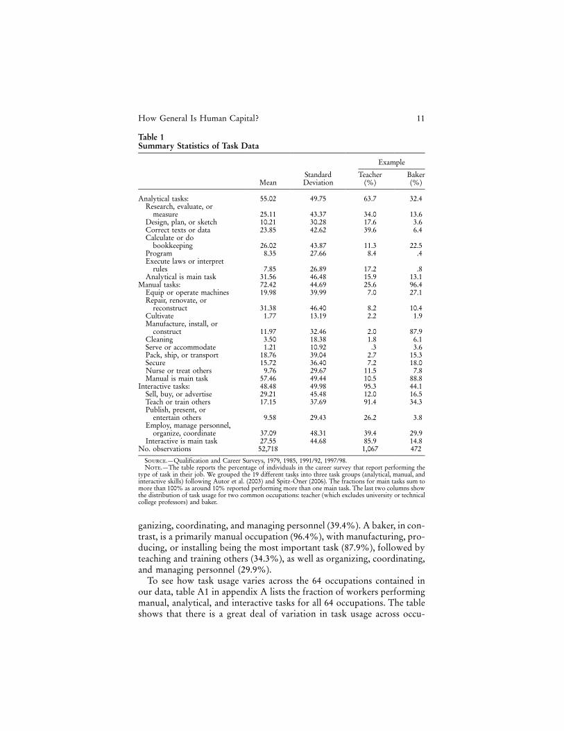
In the survey, individuals are asked whether they perform any of 19different tasks in their job. Tasks vary from repairing and cleaning tobuying and selling, teaching, and planning. For each respondent, we knowwhether he performs a certain task in his job and whether this is his mainactivity. Table 1 lists the fraction of workers performing each of the dif-ferent tasks. To simplify the exposition, we follow Autor et al. (2003) andSpitz-Oner (2006) and categorize the 19 tasks into three aggregate groups:analytical tasks, manual tasks, and interactive tasks. On average, 55%report performing analytic tasks, 72% manual tasks, and 49% interactivetasks. The picture for the main task used is similar: 32% report analyticaltasks, 57% manual tasks, and 28% interactive tasks as their main activityon the job.

The last two columns in table 1 show the distribution of tasks performedon the job for two popular occupations: teacher and baker. According toour task data, a teacher primarily performs interactive tasks (95.3%), withteaching and training others being by far the most important one (91.4%).Two other important tasks are correcting texts or data (39.6%) and or-


Table 1Summary Statistics of Task Data

MeanStandardDeviation

Example

Teacher(%)

Baker(%)

Analytical tasks: 55.02 49.75 63.7 32.4Research, evaluate, or

measure 25.11 43.37 34.0 13.6Design, plan, or sketch 10.21 30.28 17.6 3.6Correct texts or data 23.85 42.62 39.6 6.4Calculate or do

bookkeeping 26.02 43.87 11.3 22.5Program 8.35 27.66 8.4 .4Execute laws or interpret

rules 7.85 26.89 17.2 .8Analytical is main task 31.56 46.48 15.9 13.1

Manual tasks: 72.42 44.69 25.6 96.4Equip or operate machines 19.98 39.99 7.0 27.1Repair, renovate, or

reconstruct 31.38 46.40 8.2 10.4Cultivate 1.77 13.19 2.2 1.9Manufacture, install, or

construct 11.97 32.46 2.0 87.9Cleaning 3.50 18.38 1.8 6.1Serve or accommodate 1.21 10.92 .3 3.6Pack, ship, or transport 18.76 39.04 2.7 15.3Secure 15.72 36.40 7.2 18.0Nurse or treat others 9.76 29.67 11.5 7.8Manual is main task 57.46 49.44 10.5 88.8

Interactive tasks: 48.48 49.98 95.3 44.1Sell, buy, or advertise 29.21 45.48 12.0 16.5Teach or train others 17.15 37.69 91.4 34.3Publish, present, or

entertain others 9.58 29.43 26.2 3.8Employ, manage personnel,

organize, coordinate 37.09 48.31 39.4 29.9Interactive is main task 27.55 44.68 85.9 14.8

No. observations 52,718 1,067 472

Source.—Qualification and Career Surveys, 1979, 1985, 1991/92, 1997/98.Note.—The table reports the percentage of individuals in the career survey that report performing the

type of task in their job. We grouped the 19 different tasks into three task groups (analytical, manual, andinteractive skills) following Autor et al. (2003) and Spitz-Oner (2006). The fractions for main tasks sum tomore than 100% as around 10% reported performing more than one main task. The last two columns showthe distribution of task usage for two common occupations: teacher (which excludes university or technicalcollege professors) and baker.

ganizing, coordinating, and managing personnel (39.4%). A baker, in con-trast, is a primarily manual occupation (96.4%), with manufacturing, pro-ducing, or installing being the most important task (87.9%), followed byteaching and training others (34.3%), as well as organizing, coordinating,and managing personnel (29.9%).

To see how task usage varies across the 64 occupations contained inour data, table A1 in appendix A lists the fraction of workers performingmanual, analytical, and interactive tasks for all 64 occupations. The tableshows that there is a great deal of variation in task usage across occu-


pations. For example, while the average use of analytical tasks is 56.3%,the mean varies from 16.7% as an unskilled construction worker to 92.4%for an accountant. We found little evidence that tasks performed in thesame occupation vary across industries, which suggests that industriesmatter less for measuring human capital once we control for the skill setof an occupation; this justifies our focus on occupations.

B. Measuring the Distance between Occupations

According to our framework, two occupations have similar skill re-quirements if they put similar weights on tasks, that is, individuals performthe same set of tasks. With two tasks, we can measure the distance betweentwo occupations o and as the absolute difference between the weight′oeach occupation places on the first task, that is, as The basicFb � b F.′o o

idea extends naturally to the case with more than two tasks.From the task data described in the previous section, we know the set

of skills employed in each occupation. The skill content of each occupationcan then be characterized by a 19-dimensional vector, ,q p (q , … , q )o o1 oJ

where denotes the fraction of workers in an occupation performing taskqoj

j. We can think of this vector as describing a position in the task space.Occupations with a high weight in a particular task will also employboj

this task extensively, that is, have a high . To measure the distance betweenqoj

occupations in the task space, we use the angular separation or uncenteredcorrelation of the observable vectors and :q q ′o o

J� (q # q )′jo jojp1

AngSep p ,′oo J J2 2 1/2[(� q ) # (� q )]′jo kojp1 kp1

where ( ) is the fraction of workers using task j in occupation oq q ′jo jo

( ). This measure defines the distance between two occupations as the′ocosine angle between their positions in vector space. The measure hasbeen used extensively in the innovation literature to characterize the prox-imity of firms’ technologies (Jaffe 1986).9

We use a slightly modified version of the above, namely, Dis p′oo

, as our distance measure. The measure varies between zero1 � AngSep ′oo

and one. It is zero for occupations that use identical skill sets and unityif two occupations use completely different skills sets. The measure will

9 Unlike the Euclidean distance, the angular separation measure is not sensitiveto the length of the vector, i.e., whether an occupation only uses some tasks butnot others. For example, two occupations using all tasks moderately (and thus havinga position close to the origin of the coordinate system) will be similar according tothe angular separation measure even if their task vectors are orthogonal and thereforedistant according to the Euclidean distance measure. If all vectors have the samelength (i.e., if all tasks are used by at least some workers in all occupations), ourmeasure is proportional to the Euclidean distance measure.


be closer to zero the more two occupations overlap in their skill require-ments. To account for changes in task usage over time, we calculated thedistance measures separately for each wave. For the years 1975–82, weuse the measures from the 1979 cross section; for the years 1983–88, themeasures from the 1985 wave; for the years 1989–94, the measures fromthe 1991/92 wave; and for the years 1995–2001, the measures from the1997/98 wave. Our results are robust to assigning different time windowsto the measures.10

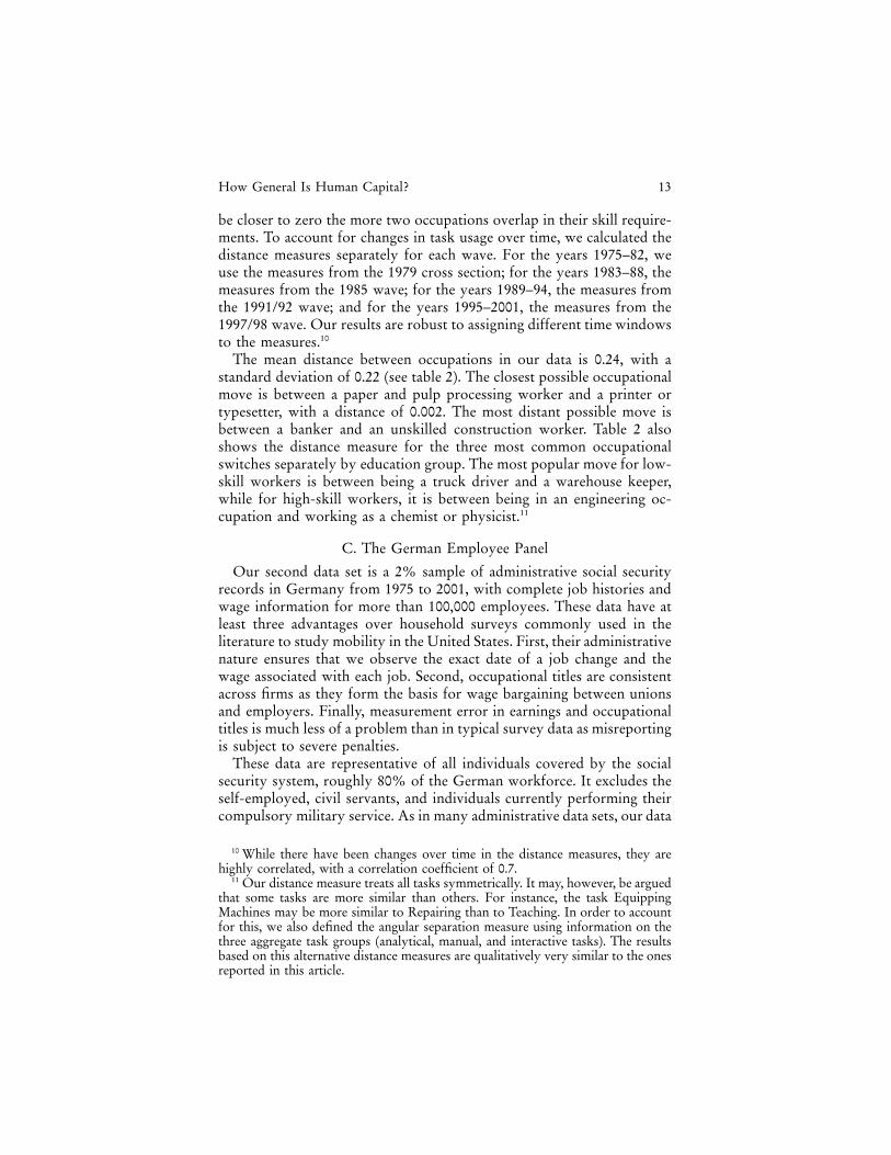
The mean distance between occupations in our data is 0.24, with astandard deviation of 0.22 (see table 2). The closest possible occupationalmove is between a paper and pulp processing worker and a printer ortypesetter, with a distance of 0.002. The most distant possible move isbetween a banker and an unskilled construction worker. Table 2 alsoshows the distance measure for the three most common occupationalswitches separately by education group. The most popular move for low-skill workers is between being a truck driver and a warehouse keeper,while for high-skill workers, it is between being in an engineering oc-cupation and working as a chemist or physicist.11

C. The German Employee Panel

Our second data set is a 2% sample of administrative social securityrecords in Germany from 1975 to 2001, with complete job histories andwage information for more than 100,000 employees. These data have atleast three advantages over household surveys commonly used in theliterature to study mobility in the United States. First, their administrativenature ensures that we observe the exact date of a job change and thewage associated with each job. Second, occupational titles are consistentacross firms as they form the basis for wage bargaining between unionsand employers. Finally, measurement error in earnings and occupationaltitles is much less of a problem than in typical survey data as misreportingis subject to severe penalties.

These data are representative of all individuals covered by the socialsecurity system, roughly 80% of the German workforce. It excludes theself-employed, civil servants, and individuals currently performing theircompulsory military service. As in many administrative data sets, our data

10 While there have been changes over time in the distance measures, they arehighly correlated, with a correlation coefficient of 0.7.

11 Our distance measure treats all tasks symmetrically. It may, however, be arguedthat some tasks are more similar than others. For instance, the task EquippingMachines may be more similar to Repairing than to Teaching. In order to accountfor this, we also defined the angular separation measure using information on thethree aggregate task groups (analytical, manual, and interactive tasks). The resultsbased on this alternative distance measures are qualitatively very similar to the onesreported in this article.

Tabl

e2

Dis

tanc

eM

easu

res

betw

een

Occ

upat

ions

(Ang

ular

Sepa

rati

on) O

ccup

atio

n1

Occ

upat

ion

2D

ista

nce

Mea

n.2

43St

anda

rdde

viat

ion

.221

Mos

tsi

mila

r(a

lled

ucat

ion

grou

ps)

Pape

ran

dPu

lpPr

oces

sing

Prin

ter,

Type

sett

er.0

02W

ood

Proc

essi

ngM

etal

Polis

her

.003

Che

mic

alPr

oces

sing

Plas

tics

Proc

essi

ng.0

04M

ost

dist

ant

(all

educ

atio

ngr

oups

)B

anke

rU

nski

lled

Con

stru

ctio

nW

orke

r.9

39B

anke

rM

iner

,Sto

ne-B

reak

er.9

36Pu

blic

ist,

Jour

nalis

tU

nski

lled

Con

stru

ctio

nW

orke

r.9

35M

ost

com

mon

occu

patio

nalm

oves

(low

-ski

lled)

Truc

kD

rive

r,C

ondu

ctor

Stor

eor

War

ehou

seK

eepe

r.0

29U

nski

lled

Wor

ker

Stor

eor

War

ehou

seK

eepe

r.2

69A

ssem

bler

Stor

eor

War

ehou

seK

eepe

r.3

69M

ost

com

mon

occu

patio

nalm

oves

(med

ium

-ski

lled)

Che

mis

t,Ph

ysic

ist

Ele

ctri

cian

,Ele

ctri

calI

nsta

llatio

n.1

71Sa

les

Pers

onne

lO

ffice

Cle

rk.0

76Tr

uck

Dri

ver,

Con

duct

orSt

ore

orW

areh

ouse

Kee

per

.028

Mos

tco

mm

onoc

cupa

tiona

lmov

es(h

igh-

skill

ed)

Eng

inee

rC

hem

ist,

Phys

icis

t.0

34E

ntre

pren

eur

Offi

ceC

lerk

.047

Acc

ount

ant

Offi

ceC

lerk

.080

No

te.—

The

top

ofth

eta

ble

prov

ides

sum

mar

yst

atis

tics

ofoc

cupa

tions

and

thei

rco

rres

pond

ing

dist

ance

.The

dist

ance

mea

sure

isth

ean

gula

rse

para

tion

usin

gth

e19

diff

eren

tta

sks

(see

tabl

e1

for

alis

toft

asks

),an

dit

isno

rmal

ized

tova

rybe

twee

n0

and

1.T

hem

iddl

epa

rtof

the

tabl

esh

ows

pair

sof

occu

patio

nalm

oves

with

the

leas

tand

grea

test

diff

eren

ces

ofdi

stan

ce.T

hebo

ttom

part

ofth

eta

ble

show

sth

eth

ree

mos

tco

mm

only

obse

rved

mov

esin

the

data

byed

ucat

ion

grou

pan

dth

eco

rres

pond

ing

dist

ance

mea

sure

.


Fig. 1.—Quarterly occupation mobility rates by time in the labor market. The figure showsthe quarterly occupation mobility rate by education and time in the labor market (potentialexperience). Mobility rates are defined over the sample of workers who are employed at thebeginning of the quarter.

are right-censored at the highest level of earnings that are subject to socialsecurity contributions. Top-coding is negligible for unskilled workers andthose with an apprenticeship, but it reaches 30% for university graduates.For the high-skilled, we use tobit or semiparametric methods to accountfor censoring.

Since the level and structure of wages differs substantially between Eastand West Germany, we drop from our sample all workers who were everemployed in East Germany. We also drop all those working in agriculture.In addition, we restrict the sample to men who entered the labor marketin or after 1975. This allows us to construct precise measures of actualexperience and firm, task, and occupation tenure from labor market entryonward. Labor market experience and our tenure variables are all mea-sured in years and exclude periods of unemployment and apprenticeshiptraining.

Occupational mobility is important in our sample: 19% of the low-skilled switch occupations each year as compared to 10% of the high-skilled. To see how occupational mobility varies over the career, figure 1plots quarterly mobility rates over the first 10 years in the labor marketseparately by education group. Occupational mobility rates are very highin the first year (particularly in the first quarter) of a career, and they are


highest for the low-skilled. Ten years into the labor market, quarterlymobility rates drop to 2%.

D. Measuring Task-Specific Human Capital

Since the concept is novel, we now explain how we calculate our mea-sure of task-specific human capital, which we term “task tenure.” Tasktenure crucially depends on the weights occupations place on tasks, .boj

We measure these occupation-specific weights as follows. First, we cal-culate the share of time workers spend in each of the 19 tasks, assumingthat they spend the same amount of time in each task they perform. Wethen average over all workers in the occupation. This ensures that theoccupation-specific weights add up to one.

We compute task tenure following equations (3) and (4) in Section II.Bwith one modification. The reason we do this is that (3) and (4) imply thattask tenure would increase by less than one unit for workers who remainin the same occupation and therefore by less than occupational tenure. Tosee this, consider again the case with two tasks and a worker who is currentlyemployed in an occupation with After 1 year, this worker hasb p 0.75.o

accumulated 0.75 units in analytical tasks and 0.25 units in manual tasks.His task tenure would increase by only 0.625 ((0.75 # 0.75) � (0.25 #

, while occupational tenure increases by one unit. Our goal, however,0.25))is to compare the return to task-specific human capital with that to generalexperience and the less portable occupation-specific skills. To ensure thiscomparability, we normalize the accumulation of task tenure for occupa-tional stayers to be one in each occupation. We do this by dividing the tasktenure accumulated in the current period by the sum of squared weightsin that occupation. This normalization also ensures that task tenure alwaysincreases more for occupational stayers than for occupational movers.

As an illustration, consider a worker in occupation A with equal weightson analytical and manual tasks ( ). After 1 year, he has accumulatedb p 0.5o

0.5 units of analytical skills and 0.5 units of manual skills (i.e., AH pi1

and . His normalized measure of task-specific human capitalM0.5 H p 0.5)i1

is then one unit ([(0.5 # 0.5) � (0.5 # 0.5)]/[(0.5 # 0.5) � (0.5 # 0.5)]).If instead he switches to occupation B with weights 0.3 on the analyticaltask and 0.7 on the manual task, his task tenure after the move declinesto 0.5 units ((0.3 # 0.5) � (0.7 # 0.5)). After a year in occupation B,his analytical and manual skills increase to HA

i2 p 0.5 � 0.3 p 0.8 andHM

i2 p 0.5 � 0.7 p 1.2 units. His overall task tenure is then 1.5 units({[(0.3 # 0.5) � (0.3 # 0.3)]/[(0.3 # 0.3) � (0.7 # 0.7)]} � {[(0.7 # 0.5)� (0.7 # 0.7)]/[(0.3 # 0.3) � (0.7 # 0.7)]}). The first (second) term incurly brackets denotes the contribution of analytical (manual) skills inoccupation A and B to total task tenure. This normalization ensures thattask tenure is at least as large as occupational tenure (since occupation-

gathmann

Highlight


Table 3Summary Statistics of West German Employee Panel

Low-Skilled Medium-Skilled High-Skilled

Percentage in sample (%) 17.82 67.87 14.31Age (in years) 25.81 27.47 31.88

(6.03) (5.23) (5.27)Not German citizen (%) 34.42 5.29 5.19Median daily wage 113.78 135.32 206.74

(44.97) (43.33) (60.23)Log daily wage 4.66 4.89 5.20

(.45) (.33) (.42)Percentage censored 1.17 2.39 30.00Actual experience (in years) 5.67 5.58 4.96

(5.34) (4.75) (4.58)Occupational tenure (in years) 2.93 3.61 3.34

(4.09) (4.04) (3.88)Firm tenure (in years) 2.44 2.80 2.43

(3.84) (3.66) (3.25)Task tenure (in years) 3.23 3.57 3.90

(3.02) (2.92) (3.44)Occupational mobility .19 .11 .10Distance of move .28 .24 .16

(.23) (.22) (.18)Firm mobility .24 .18 .17Most common occupations Warehouse Keeper Electrical Installation Engineer

Assembler Locksmith TechnicianConductor Mechanic, Machinist AccountantUnskilled Worker Office Clerk Office ClerkOffice Clerk Conductor Scientist, Clergyman

No. observations 244,759 1,003,823 172,930No. individuals 20,846 79,396 16,735

Source.—Employee Sample (Institute for Labor Market Research [IAB]), 1975–2001.Note.—The table reports means and standard deviations (in parentheses) for the administrative panel

data on individual labor market histories and wages from 1975 to 2001. Low-skilled are those withouta vocational degree, medium-skilled have either a high school or vocational degree, and high-skilled havean advanced degree from a technical college or university. Experience, occupational tenure, and task andfirm tenure are measured from actual spells and exclude periods of unemployment or being out of thelabor force. The wage is measured in German marks at 1995 prices and is subject to right-censoring.

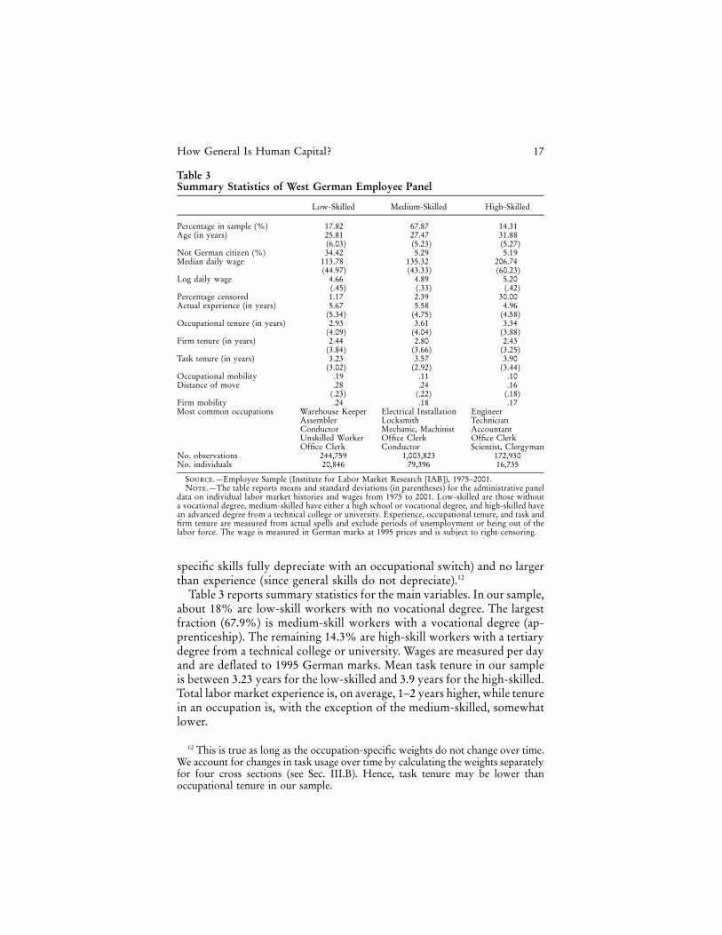
specific skills fully depreciate with an occupational switch) and no largerthan experience (since general skills do not depreciate).12

Table 3 reports summary statistics for the main variables. In our sample,about 18% are low-skill workers with no vocational degree. The largestfraction (67.9%) is medium-skill workers with a vocational degree (ap-prenticeship). The remaining 14.3% are high-skill workers with a tertiarydegree from a technical college or university. Wages are measured per dayand are deflated to 1995 German marks. Mean task tenure in our sampleis between 3.23 years for the low-skilled and 3.9 years for the high-skilled.Total labor market experience is, on average, 1–2 years higher, while tenurein an occupation is, with the exception of the medium-skilled, somewhatlower.

12 This is true as long as the occupation-specific weights do not change over time.We account for changes in task usage over time by calculating the weights separatelyfor four cross sections (see Sec. III.B). Hence, task tenure may be lower thanoccupational tenure in our sample.


IV. Patterns in Occupational Mobility and Wages

We now use the sample of occupational movers to provide descriptiveevidence that skills are partially transferable across occupations. Whilethe patterns shown below are not a rigorous test, they are all consistentwith our task-based approach. Section IV.A studies mobility behavior,while Section IV.B analyzes wages before and after an occupational move.

A. Occupational Moves Are Similar

Our framework predicts that workers are more likely to move to oc-cupations with similar task requirements. In contrast, if skills are eitherfully general or fully specific to an occupation, they do not influence thedirection of occupational mobility: in the first case human capital can beequally transferred to all occupations, while in the second case humancapital fully depreciates irrespective of the target occupation.

To test this hypothesis, we compare the distance of observed moves tothe distribution of occupational moves we would observe if the directionof occupational moves were random. In particular, we assume that, underrandom mobility, the decision to move to a particular occupation is solelydetermined by its relative size. For example, if occupation A employstwice as many workers as occupation B, the probability that a workerjoins occupation A would then be twice as high as the probability thathe joins occupation B. The way we calculate random mobility ensuresthat we account for shifts in the occupational structure over time, thatis, the fact that employment shares may be increasing or decreasing forsome occupations.13

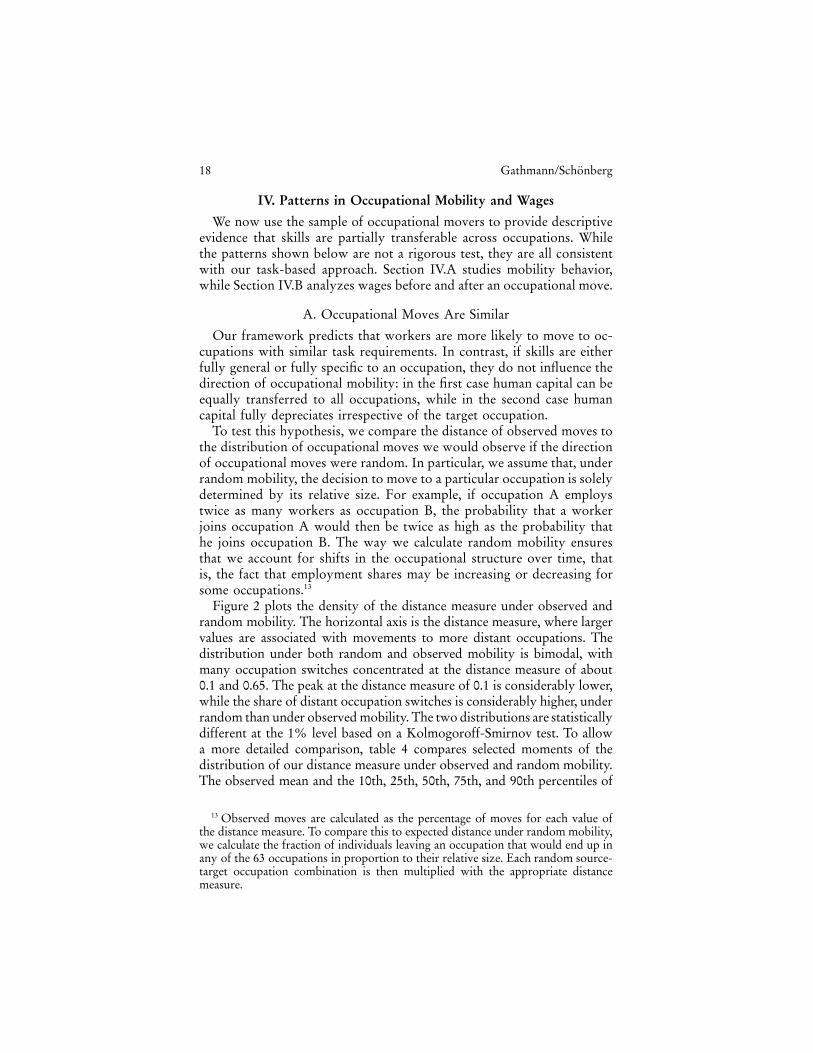
Figure 2 plots the density of the distance measure under observed andrandom mobility. The horizontal axis is the distance measure, where largervalues are associated with movements to more distant occupations. Thedistribution under both random and observed mobility is bimodal, withmany occupation switches concentrated at the distance measure of about0.1 and 0.65. The peak at the distance measure of 0.1 is considerably lower,while the share of distant occupation switches is considerably higher, underrandom than under observed mobility. The two distributions are statisticallydifferent at the 1% level based on a Kolmogoroff-Smirnov test. To allowa more detailed comparison, table 4 compares selected moments of thedistribution of our distance measure under observed and random mobility.The observed mean and the 10th, 25th, 50th, 75th, and 90th percentiles of

13 Observed moves are calculated as the percentage of moves for each value ofthe distance measure. To compare this to expected distance under random mobility,we calculate the fraction of individuals leaving an occupation that would end up inany of the 63 occupations in proportion to their relative size. Each random source-target occupation combination is then multiplied with the appropriate distancemeasure.


Fig. 2.—Observed mobility is more similar than random mobility. The figure plots thedensity of the distance measure under observed and random mobility. We calculate randommobility as follows: for each mover, we assume that the probability of going to any otheroccupation in the data is solely determined by the relative size of the target occupation. Wethen multiply this “random move” with its distance to get the distribution of the distancemeasure under random mobility. Distance measure is angular separation, based on 19 tasks.

the distance distribution are much lower than what we would observe underrandom mobility.

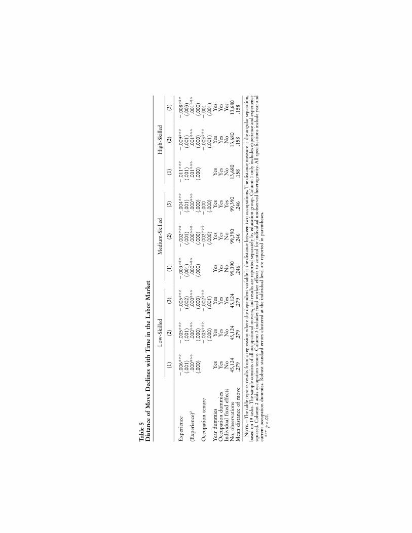
Our framework also predicts that distant moves occur early in the labormarket career and that moves become increasingly similar with time inthe labor market. Table 5 provides empirical support for these predictions.It shows the results from a linear regression where the dependent variableis the distance of an observed move separately by education group. Weinclude experience and experience squared as well as year and occupationfixed effects as controls. Occupation dummies control for the occupation-specific skill price in the occupation, which might be correlated with( p )o

experience or directly with the distance measure.14 Year fixed effects ac-count for aggregate shocks to the economy.

For all education groups, the distance of an occupational move declineswith time spent in the labor market, although it does so at a decreasing

14 We find that workers in occupations that pay higher wages (i.e., employ ahigher average skill level) also have higher task tenure and move to more similaroccupations. The occupation dummies control for these correlations and hence avoidoverestimating the relationship between experience and distance of move or distanceand wages in the next section.


Table 4Observed Moves Are More Similar than underRandom Mobility

Random Mobility Observed Mobility

Mean .466 .406Percentile:

10th .083 .04725th .267 .12250th .507 .38175th .668 .59790th .776 .679

Note.—The table reports selected moments of the distribution of observedoccupational moves (Observed Mobility) and compares it against what wewould expect to observe under random mobility (Random Mobility). We cal-culate random mobility as follows: for each mover, we assume that the prob-ability of going to any other occupation in the data is solely determined by therelative size of the target occupation. We then multiply this “random move”with its distance to get the distribution of the distance measure under randommobility. The distance measure is the angular separation, based on 19 tasks.Since all moments of the observed distribution are below those under randommobility, individuals are much more likely to move to a similar occupation.

rate. After 10 years in the labor market, the distance of an occupationalmove declines by 0.03 for the low-skilled and medium-skilled and by asmuch as 0.10 for the high-skilled. Given the coefficients in specification1 of table 5, actual labor market experience can account for up to two-thirds of this decline.

Time spent in the previous occupation also decreases the distance ofan occupational move in addition to labor market experience (col. 2).Column 3 reports the results from a fixed effects estimator, which is usedin order to control for heterogeneity in mobility behavior across indi-viduals. The within estimator shows that occupational moves becomemore similar even for the same individual over time. If anything, thepattern of declining distance is more pronounced in the fixed effectsestimation.

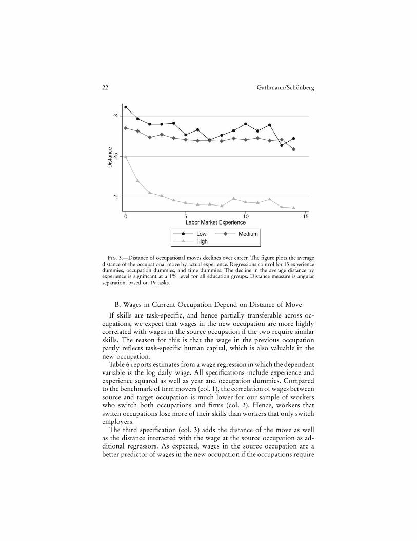
The specification reported in table 5 imposed a quadratic relationshipbetween actual labor market experience and the distance of moves. Infigure 3, we relax this restriction. The figure displays, separately for thethree education groups, the average distance of a move by actual expe-rience. The average distance is obtained from a least squares regressionof the distance on dummies for actual experience as well as occupationand year dummies, similar to column 1 in table 5. The figure shows thatoccupational moves become more similar with time in the labor marketfor all education groups but that is particularly so for the high-skilled inthe first 5 years in the labor market. The decline in distance between thefirst and fifteenth year of actual labor market experience is statisticallysignificant at the 1% level for all education groups.

Tabl

e5

Dis

tanc

eof

Mov

eD

eclin

esw

ith

Tim

ein

the

Lab

orM

arke

t

Low

-Ski

lled

Med

ium

-Ski

lled

Hig

h-Sk

illed

(1)

(2)

(3)

(1)

(2)

(3)

(1)

(2)

(3)

Exp

erie

nce

�.0

06**

*�

.005

***

�.0

05**

*�

.003

***

�.0

02**

*�

.004

***

�.0

11**

*�

.009

***

�.0

08**

*(.0

01)

(.001

)(.0

02)

(.001

)(.0

01)

(.001

)(.0

01)

(.001

)(.0

03)

(Exp

erie

nce)

2.0

00**

*.0

00**

*.0

00**

*.0

00**

*.0

00**

*.0

00**

*.0

01**

*.0

01**

*.0

01**

*(.0

00)

(.000

)(.0

00)

(.000

)(.0

00)

(.000

)(.0

00)

(.000

)(.0

00)

Occ

upat

ion

tenu

re�

.003

***

�.0

02**

*�

.002

***

�.0

00�

.003

***

�.0

01(.0

00)

(.001

)(.0

00)

(.000

)(.0

01)

(.001

)Y

ear

dum

mie

sY

esY

esY

esY

esY

esY

esY

esY

esY

esO

ccup

atio

ndu

mm

ies

Yes

Yes

Yes

Yes

Yes

Yes

Yes

Yes

Yes

Indi

vidu

alfi

xed

effe

cts

No

No

Yes

No

No

Yes

No

No

Yes

No.

obse

rvat

ions

45,1

2445

,124

45,1

2499

,390

99,3

9099

,390

13,6

8013

,680

13,6

80M

ean

dist

ance

ofm

ove

.279

.279

.279

.246

.246

.246

.158

.158

.158

No

te.—

The

tabl

ere

port

sre

sult

sfr

oma

regr

essi

onw

here

the

depe

nden

tva

riab

leis

the

dist

ance

betw

een

two

occu

pati

ons.

The

dist

ance

mea

sure

isth

ean

gula

rse

para

tion

,ba

sed

on19

task

s.T

hesa

mpl

eco

nsis

tsof

allo

ccup

atio

nalm

over

s,an

dre

sult

sar

ere

port

edse

para

tely

byed

ucat

ion

grou

p.C

olum

n1

only

incl

udes

expe

rien

cean

dex

peri

ence

squa

red.

Col

umn

2ad

dsoc

cupa

tion

tenu

re.C

olum

n3

incl

udes

fixe

dw

orke

ref

fect

sto

cont

rolf

orin

divi

dual

unob

serv

edhe

tero

gene

ity.

All

spec

ifica

tion

sin

clud

eye

aran

dcu

rren

toc

cupa

tion

dum

mie

s.R

obus

tst

anda

rder

rors

clus

tere

dat

the

indi

vidu

alle

vel

are

repo

rted

inpa

rent

hese

s.**

*p

!.0

1.


Fig. 3.—Distance of occupational moves declines over career. The figure plots the averagedistance of the occupational move by actual experience. Regressions control for 15 experiencedummies, occupation dummies, and time dummies. The decline in the average distance byexperience is significant at a 1% level for all education groups. Distance measure is angularseparation, based on 19 tasks.

B. Wages in Current Occupation Depend on Distance of Move

If skills are task-specific, and hence partially transferable across oc-cupations, we expect that wages in the new occupation are more highlycorrelated with wages in the source occupation if the two require similarskills. The reason for this is that the wage in the previous occupationpartly reflects task-specific human capital, which is also valuable in thenew occupation.

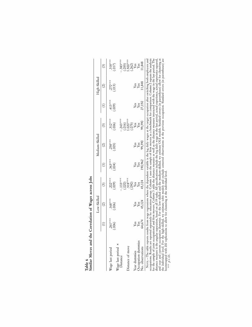
Table 6 reports estimates from a wage regression in which the dependentvariable is the log daily wage. All specifications include experience andexperience squared as well as year and occupation dummies. Comparedto the benchmark of firm movers (col. 1), the correlation of wages betweensource and target occupation is much lower for our sample of workerswho switch both occupations and firms (col. 2). Hence, workers thatswitch occupations lose more of their skills than workers that only switchemployers.

The third specification (col. 3) adds the distance of the move as wellas the distance interacted with the wage at the source occupation as ad-ditional regressors. As expected, wages in the source occupation are abetter predictor of wages in the new occupation if the occupations require

Tabl

e6

Sim

ilar

Mov

esan

dth

eC

orre

lati

onof

Wag

esac

ross

Jobs

Low

-Ski

lled

Med

ium

-Ski

lled

Hig

h-Sk

illed

(1)

(2)

(3)

(1)

(2)

(3)

(1)

(2)

(3)

Wag

ela

stpe

riod

.261

***

.168

***

.202

***

.363

***

.258

***

.312

***

.413

***

.270

***

.318

***

(.006

)(.0

06)

(.009

)(.0

04)

(.005

)(.0

06)

(.009

)(.0

13)

(.017

)W

age

last

peri

od#

Dis

tanc

e�

.133

***

�.2

43**

*�

.383

***

(.020

)(.0

16)

(.055

)D

ista

nce

ofm

ove

.518

***

1.02

0***

1.50

0***

(.090

)(.0

75)

(.262

)Y

ear

dum

mie

sY

esY

esY

esY

esY

esY

esY

esY

esY

esO

ccup

atio

ndu

mm

ies

Yes

Yes

Yes

Yes

Yes

Yes

Yes

Yes

Yes

No.

obse

rvat

ions

64,6

7445

,124

45,1

2419

0,96

299

,390

99,3

9027

,150

11,8

4811

,848

No

te.—

The

tabl

ere

port

sre

sult

sfr

omw

age

regr

essi

ons

whe

reth

ede

pend

ent

vari

able

isth

elo

gda

ilyw

ages

atth

eta

rget

occu

pati

onaf

ter

swit

chin

gbo

them

ploy

ers

and

occu

pati

ons.

Res

ults

are

repo

rted

sepa

rate

lyby

educ

atio

ngr

oup.

Col

umn

1us

esth

esa

mpl

eof

firm

mov

ers

asa

benc

hmar

kfo

rco

mpa

riso

n.C

olum

n2

repe

ats

the

anal

ysis

for

the

sam

ple

ofjo

int

occu

pati

onal

and

firm

mov

ers.

Col

umn

3ad

dsth

edi

stan

cem

easu

reas

wel

las

the

dist

ance

mea

sure

inte

ract

edw

ith

the

wag

ein

the

last

peri

od.T

hedi

stan

cem

easu

reis

the

angu

lar

sepa

rati

on,b

ased

onal

l19

task

s.A

llsp

ecifi

cati

ons

incl

ude

the

log

daily

wag

ein

the

last

peri

od,a

ctua

lexp

erie

nce,

actu

alex

peri

ence

squa

red,

and

year

and

curr

ent

occu

pati

ondu

mm

ies.

For

the

low

-ski

lled

and

the

med

ium

-ski

lled,

we

esti

mat

eO

LS

mod

els.

Stan

dard

erro

rs(i

npa

rent

hese

s)al

low

for

clus

teri

ngat

the

indi

vidu

alle

vel.

For

the

high

-ski

lled,

we

esti

mat

eto

bit

mod

els

and

excl

ude

cens

ored

obse

rvat

ions

atth

epr

evio

usoc

cupa

tion

.St

anda

rder

rors

(in

pare

nthe

ses)

are

boot

stra

pped

with

200

repl

icat

ions

toal

low

for

clus

teri

ngat

the

indi

vidu

alle

vel.

***

p!

.01.


Table 7Past Occupational Tenure Matters for Wages

Low-Skilled Medium-Skilled High-Skilled

(1) (2) (1) (2) (1) (2)

Past occupational tenure .014*** .015*** .013*** .014*** .024*** .026***(.001) (.001) (.001) (.001) (.002) (.003)

Past tenure # Distance �.007* �.006*** �.037***(.004) (.002) (.011)

Distance of move �.086*** �.133*** �.358***(.010) (.007) (.030)

Year dummies Yes Yes Yes Yes Yes YesOccupational dummies Yes Yes Yes Yes Yes YesNo. observations 45,124 45,124 99,390 99,390 13,680 13,680

Note.—The table reports wage regressions where the dependent variable is the log wages in the targetoccupation after switching both employers and occupations. Column 1 in each specification controls forpast tenure in the source occupation, experience, experience squared, and year and current occupationdummies. Column 2 additionally includes the distance measure and its interaction with past occupationaltenure. The distance measure used is the angular separation, based on all 19 tasks. For the low-skilledand the medium-skilled, we report results from OLS regressions. Standard errors (in parentheses) allowfor clustering at the individual level. For the high-skilled, we estimate tobit models. Here, standard errors(in parentheses) are bootstrapped with 200 replications to account for clustering at the individual level.

* p ! .10.*** p ! .01.

similar skills. For the high-skilled, our estimates imply that the correlationof the wage at the source occupation and the wage at the target occupationis 0.26 for the mean move but only 0.12 for a(0.318 � (0.383 # 0.158))distant (90th percentile) move (0.318 � (0.383 # 0.507)).

If skills are partially transferable across occupations, then time spentin the last occupation should also matter for wages in the new occupation,especially if the two occupations require similar skills. In column 1 oftable 7, we regress wages at the new occupation on occupational tenureat the previous occupation and the same controls as before. Past occu-pational tenure positively affects wages at the new occupation. Column2 adds the distance measure interacted with past occupational tenure ascontrols. As expected, the predictive power of past occupational tenureis stronger if source and target occupations are similar, especially foruniversity graduates. For this education group, the impact of past oc-cupational tenure on wages is 2.6% for the most similar move and around2% for the mean distance move.(0.026 � (0.037 # 0.158))

The specification in figure 4a relaxes the assumption that the correlationbetween wages across occupations declines linearly with the distance. Thex-axis shows the distance, with 1 being the most similar occupationalmoves and 10 the most distant ones, while the y-axis reports the coefficienton the wage in the source occupation for each of the 10 categories.15

15 The coefficient is obtained form an OLS regression (tobit regression for thehigh-skilled) that controls for actual experience, actual experience squared, yeardummies, the wage at the source occupation, nine dummies for the distance of the

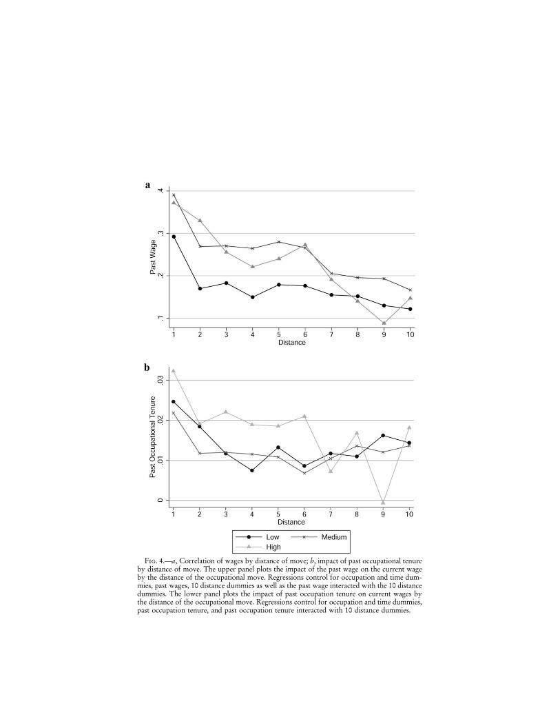
Fig. 4.—a, Correlation of wages by distance of move; b, impact of past occupational tenureby distance of move. The upper panel plots the impact of the past wage on the current wageby the distance of the occupational move. Regressions control for occupation and time dum-mies, past wages, 10 distance dummies as well as the past wage interacted with the 10 distancedummies. The lower panel plots the impact of past occupation tenure on current wages bythe distance of the occupational move. Regressions control for occupation and time dummies,past occupation tenure, and past occupation tenure interacted with 10 distance dummies.


Figure 4b presents results from a similar analysis for past occupationaltenure. The y-axis now shows, for each of the 10 distance categories, thecoefficients on occupational tenure in the source occupation from a (tobit)wage regression that also controls for actual experience, actual experiencesquared, and year dummies.

Two things are noteworthy. First, the figures highlight that wages inthe source occupation are more strongly related to wages at the targetoccupation if the source and the target occupation have similar skill re-quirements. Second, and in line with our results on mobility and wages,the decline in the relationship is strongest for the high-skilled. For thiseducation group, the partial correlation coefficient between wages in thesource and target occupation drops from 38% for the 10% most similarmoves to around 14% for the 10% most distant moves. The drop isstatistically significant at a 1% level for all education groups.

We performed a number of robustness checks. First, results for alter-native distance measures are very similar. Furthermore, our original sam-ple of movers contains everybody switching occupations irrespective ofthe duration of intermediate unemployment or nonemployment spells.To account for potential heterogeneity between those remaining out ofemployment for an extended period of time and job-to-job movers, wereestimated the results only for the sample of workers with intermediateunemployment or nonemployment spells of less than a year. Again, thisdoes not change the observed patterns in mobility and wages.

C. Can These Patterns Be Explained by Unobserved Heterogeneity?

This section discusses whether the patterns in mobility and wages foundin the last section are consistent with other forms of unobserved hetero-geneity. Note, first, that all results presented above are based on a sampleof occupational movers. Hence, the observed patterns cannot be accountedfor by a simple mover-stayer model, where movers have a higher prob-ability of leaving a job and therefore lower productivity because of lessinvestment in specific skills. To the extent that movers differ from stayersin terms of observable and unobservable characteristics, this sample re-striction reduces selection bias.

Other sources of unobserved heterogeneity could, however, bias our re-sults. First, suppose that high-ability workers are less likely to switch oc-cupations. This could account for the fact that the time spent in the lastoccupation has a positive effect on wages in the current occupation as pastoccupational tenure would act as a proxy for unobserved ability in the wageregression (see table 7). However, unobserved ability per se cannot explain

move, and the nine dummies interacted with the wage at the source occupation (seecol. 3 in table 6).


why the effect of past occupational tenure should vary with the distance ofthe move or why individuals move to similar occupations at all.

Second, one might argue that similar moves in the data are voluntarytransitions, while distant movers are “lemons” who are laid off from theirprevious job and cannot find jobs in similar occupations. The distinctionbetween quits and layoffs could explain why wages are more highly correlatedacross similar occupations or why past occupational tenure has a higher returnin a similar occupation. However, the distinction between voluntary andinvoluntary movers cannot explain why voluntary movers choose similaroccupations in the first place. We checked whether our results differ betweenjob-to-job movers, who are more likely to be moving voluntary, and job-to-unemployment transitions, which are more likely to be involuntary. Whilethe distance of moves is lower for job-to-job transitions, we find similarpatterns for mobility and wages even for the two types of movers.

Finally, suppose that the sample of movers differs in their taste for particulartasks. Some individuals prefer research over negotiating, while others favornegotiating over managing personnel, and so forth. Taste heterogeneity canexplain why we see similar moves in the data. However, a story based ontaste heterogeneity alone cannot explain why wages are more strongly cor-related between similar occupations. If there are compensating wage differ-entials, we would actually expect the opposite result: individuals would bewilling to accept lower wages in an occupation with their preferred task mix.

This discussion highlights that a simple story of unobserved hetero-geneity cannot account for all of the results presented above. The nextsection outlines an estimation approach to quantify the importance oftask-specific human capital for individual wage growth that takes intoaccount workers’ decisions of whether to switch occupations and whetherto move to a close or distant occupation.

V. Task-Specific Human Capital and Individual Wage Growth

A. Econometric Model

To estimate the contribution of task-specific human capital to individualwage growth, we start from the log-wage regression (eq. [5]) in SectionII, augmented by other forms of human capital:

ln w p a Exp � g T � d O � l F � � , (7)ioft o it o iot o iot o ift ioft

where denotes actual experience and task tenure, with theirExp Tit iot

respective returns and As specific human capital, we include oc-a g .o o

cupation tenure and firm tenure , with returns and , respec-O F d liot ift o o

tively. Note that we allow the return to all forms of human capital ac-cumulation to be occupation-specific. This specification takes seriouslythe existing empirical evidence that returns to labor market skills differ


across occupations (e.g., Heckman and Sedlacek 1985; Gibbons et al.2005).

The unobserved (for the econometrician) error term has the fol-�ioft

lowing components:A M� p v � b t � (1 � b )t � m � u . (8)ioft i o i o i if ioft

The first term represents individual ability that is equally valued acrossall occupations, is the task-specific match in an occu-A Mb t � (1 � b )to i o i

pation, and denotes the firm match between worker i and employermif

Finally, is an independent and identically distributed error termf. uioft

capturing, for example, measurement error in wages.Our goal is to estimate the average returns of the different forms of

human capital and to compare their relative contributions to individualwage growth. To understand the selection issues involved in the estimation,we can rewrite equations (7) and (8) as a random coefficient model:

ln w p aExp � gT � dO � lF � e ,¯ioft it iot iot ift ioft

′ A Me p p X � v � [b t � (1 � b )t ] � m � u , (9)ioft o ioft i o i o i if ioft

where and′ ′X p [Exp T O F ] p p [(a � a) (g � g) (d � d)¯ioft it iot iot ift o o o o

The unobserved error term now contains an additional term(l � l)]. eo ioft

capturing the occupational heterogeneity in the returns to human capital.Suppose, first, that returns to observable human capital are constant

across occupations. Then, equals zero, which rules out that′p Xo ioft

workers sort into occupations based on the returns to human capital.Estimating equation (9) without the term by least squares results′p Xo ioft

in three biases due to unobserved ability , occupational matches(v )i( ), and firm matches . We would expect the returnA Mb t � (1 � b )t (m )o i o i if

to experience, to be upward biased because workers locate bettera,occupational and firm matches with time in the labor market throughon-the-job search. The return to experience therefore reflects not onlyaccumulation of general human capital but also wage growth due to jobsearch. Similarly, workers with higher ability (higher ) are typically morevi

attached to the labor market, which creates an additional upward bias. Incontrast, the returns to occupation-specific and task-specific human cap-ital, g and may be upward or downward biased. On the one hand,d,workers with a good occupation or firm match are typically less likelyto switch occupations, which produces a positive (partial) correlation be-tween occupation and task tenure and the match terms. On the otherhand, workers may have switched to a new occupation or moved to adistant occupation because they found a particularly good occupation orfirm match, which implies a downward bias in the return to occupation-specific and task-specific human capital. Moreover, high-ability workersmay be less likely to switch occupations in general, or to switch to distant


occupations, creating an additional upward bias in the return to occu-pational and task tenure.

In the more general case with heterogeneous returns , we′(p X ( 0)o ioft

will have an additional source of bias because workers sort themselvesinto occupations based on the returns to human capital. Sorting accordingto comparative advantage is another reason why the (partial) bias in thereturn to occupation and task tenure cannot be signed. We next outlineour estimation approach to address these selection issues.

B. Estimation Approach

Our first step to get consistent estimates of the average returns to humancapital is to use a sample of workers who were exogenously displacedfrom their job due to plant closure (see Gibbons and Katz [1991], Neal[1995], and Dustmann and Meghir [2005] for a similar strategy). Exog-enously displaced workers lost their current firm match and need to startsearching for a new employer from scratch. Such workers are willing toaccept a new job offer if its value exceeds the value of unemployment.In contrast, voluntary job switchers are only observed because the valueof the new job exceeds that of the old job. Hence, using the sample ofexogenously displaced workers eliminates the upward bias in the returnsto general human capital from improved firm matches ( ) because theirmif

firm match after reemployment is a random sample of the working pop-ulation conditional on the observable characteristics.16 Note that this con-dition only holds for the first period after the displaced worker has beenreemployed. Therefore, our sample of displaced workers is based on thisfirst period alone. Since firm tenure is zero in this sample, we cannotestimate the return to firm tenure, and we therefore drop the term

from the wage equation (9).17l Fo ift

The returns to experience, occupational tenure, and task tenure are thenprimarily identified from the cross-sectional comparison of displacedworkers with different years of accumulated human capital. Estimatingwage equation (9) with fixed effects for the displaced sample (and henceexploiting that some workers were displaced more than once) will absorbthe individual ability term . This approach reduces the possible upwardvi

bias in the returns to experience, occupation tenure, and task tenure dueto a positive (partial) correlation between these variables and ability. How-ever, the fixed effect approach does not solve the problem of endogenous

16 Dustmann and Meghir (2005) provide evidence that the assumption of plantclosure as an exogenous job loss is reasonable in the German context.

17 The same restriction applies to our sample of voluntary firm switchers. Thatsample also has a firm tenure of zero, and we therefore cannot estimate the returnto firm tenure for this group.


selection into occupations based on the task match and heterogeneousreturns to observable human capital.

To address these selection issues, we rely on a control function ap-proach. The basic idea is to explicitly model the conditional mean of theerror term in (9) and then include its empirical counterpart as a controlvariable in the estimation of the wage equation (see Heckman and Vytlacil[1998] for the general setup).18 For consistent estimates, the control func-tion approach requires the following assumptions. First, the instrumentsneed to satisfy a rank condition. Economically, this implies that the in-struments affect the worker’s mobility decision, that is, whether to moveto a new occupation and whether to move to a similar or distant occu-pation conditional on the observables and other exogenous controls. Sec-ond, the instruments must be uncorrelated with the error term in theZiot

wage equation conditional on our exogenous control variables (time, oc-cupation, and region dummies that we include in all specifications below).Formally, the exclusion restrictions are

A M ˜E[{v � b t � (1 � b )t } � m � u FX , Z ] p 0,i o i o i if ioft iot iot

˜ ˜E[(a � a)FX , Z ] p E[(g � g)FX , Z ]¯o iot iot o iot iot

˜p E[(d � d)FX , Z ] p 0,o iot iot

where denotes the set of exogenous controls (and hence does not includeXiot

our potentially endogenous human capital variables Our main in-X ).iot

struments for experience are age and age squared. To instrument for oc-cupation tenure, we follow Altonji and Shakotko (1987) and Parent (2000)and use the deviation of individual occupation tenure from its occupation-specific mean as an instrument. This instrument is uncorrelated with ability,

and the time-invariant task match, by construction.19A Mv , b t � (1 � b )t ,i o i o i

18 Note that a linear instrumental variable strategy will not identify the averagereturn to human capital in this case except in very special circumstances. In particular,we would need to assume that the instruments are uncorrelated with the occupation-specific deviations from the average return and also are uncorrelated with the in-dividual task match conditional on our observable human capital variables and otherexogenous controls.

19 Note that the deviation of occupation tenure from its occupation-specific meandoes not eliminate a possible correlation with the firm-specific match component.This is likely to lead to a downward bias in the returns to occupation as workersmay switch occupations and lose occupation-specific human capital because theysecured a particularly good firm match. It is also likely to lead to a downward biasin the return to task-specific human capital as, among occupation switchers, workersmay switch to a distant occupation and lose more task-specific human capital becauseof a good firm match. The sample restriction to consider only exogenously displacedworkers should weaken this trade-off between specific human capital and a goodfirm match, but it may not completely eliminate it. A second reason why we expect


For task tenure, we use local labor market conditions, in particular thesize of occupation and the average distance to other occupations in thesame local labor market, as well as both variables interacted with age, asinstruments.20 The basic idea is that workers who have more employmentopportunities in their original occupation, or similar such occupations,will be less likely to switch occupations or move to a distant occupation.Conditional on occupation, region, and time dummies, the variation weexploit is changes in the occupational structure over time within the sameregion. These changes will not affect wages if occupation-specific factorprices are equalized across local labor markets. Hence, our assumptionrequires that occupation-specific wages be set in a national labor market(see Adda et al. [2006] for a similar argument).

Finally, the following control function assumptions need to hold:

Exp T O˜E[(a � a)FX , X , Z ] p f(v , v , v ),¯o iot iot iot

Exp T O˜E[(g � g)FX , X , Z ] p g(v , v , v ), (10)o iot iot iot

Exp T O˜E[(d � d)FX , X , Z ] p h(v , v , v ),o iot iot iot

andA M Exp T OE[{v � b t � (1 � b )t } � m � u FX , Z ] p k(v , v , v ), (11)i o i o i ift ioft iot iot

where , andExp Tv p Exp � E[Exp FX , Z ], v p T � E[T FX , Z ]it it iot iot iot iot iot iot

are the residuals from the respective reducedOv p O � E[O FX , Z ]iot iot iot iot

forms and and are linear in their arguments.21 The firstf (7) , g (7) , h (7) , k (7)set of conditions (see [10]) accounts for sorting based on the occupation-specific returns to human capital, while the last assumption (see [11])accounts for selection into occupations based on task match quality.

To implement the control function estimator, we first estimate the re-duced forms for experience, occupational tenure, and task tenure andpredict the residuals. The results are shown in table A2 in appendix A

this bias to be small is that the majority of young workers in our sample have beenin the labor market for less than 8 years, so their decisions whether to switchoccupations and to which occupation to move should be predominantly driven bythe task match and not by the firm match (Neal 1999).

20 The average distance, , to other occupations is computed separately forADrt

each local labor market r and time period t as follows: 64AD p � Prop #′′rt rtoo (o

The first term denotes the proportion of workers in occupation in′Distance . o′oo

year t and regional labor market r; the second term describes the distance betweenoccupations o and . We define a region as the individual’s county (Kreis) of res-′oidence as well as all the neighboring counties, corresponding roughly to a 50 mileradius from the individual’s home.

21 Note that the identification of the control function approach does not hingeon these linearity assumptions. See Florens et al. (2008) for a discussion of non-parametric identification of the control function estimator.


for the low-skilled and medium-skilled and in table A3 (also in app. A)for the high-skilled. In the second step, we estimate the log wage equationin (9) including the estimated residuals as well as their interaction withthe endogenous regressors. The latter controls for selection based onheterogeneous returns to human capital. For the high-skilled, we use thesemiparametric estimator proposed by Blundell and Powell (2004) to ac-count for censoring in addition to endogenous regressors. We describethis estimator in detail in appendix B. Since this estimator identifies theslope of the conditional quantile function and imposes common returnson the observable human capital variables, the estimates are not directlycomparable to those of the other education groups or the least squaresestimates in table 8. We bootstrap standard errors with 200 replicationsusing the individual as the sampling unit in order to correct for generatedregressor bias.

C. Empirical Results

We first report our benchmark least squares results; for university grad-uates, we estimated censored regression models to account for top-codedwages. Table 8 reports results first for the whole sample and then for thesample of firm switchers and displaced workers. The odd columns displayresults from a wage regression that ignores task-specific human capital,while the results presented in the even columns are from a specificationthat includes task tenure as an additional regressor.

The results in columns 1–6 reveal several interesting patterns. Returns totask tenure are sizable and exceed those of occupational tenure for alleducation groups. A second interesting result is that the returns to occu-pation-specific and general human capital decline once we account for task-specific human capital. For example, for the high-skilled who were displacedfrom their firm (cols. 5 and 6), returns to occupational tenure decline from1.7% to 0.6% and returns to experience become negligible.

Since least squares estimates are biased, we now turn to two alternativeestimators of the wage equation in table 9. We first show the fixed effectsestimates for the displaced sample (cols. 1 and 2). This specification elim-inates an upward bias in the return to experience from search over firmmatches as well as from unobserved ability that is equally valued acrossoccupations. For university graduates, we use the trimming estimator forcensoring (Type 1 tobit model) with fixed effects proposed by Honore(1992).22 For the low-skilled and the medium-skilled, results are similarto the OLS estimates for the same sample. For the high-skilled, estimatesare very noisy, so no firm conclusion can be drawn.

22 Since the estimator is semiparametric, no functional form assumption on theerror term is required. However, we do require pairwise exchangeability of the errorterms conditional on the included regressors (see Honore [1992] for details).


Table 8Returns to Labor Market Skills: Least Squares Estimates

Whole Sample Firm Switchers Displaced Workers

(1) (2) (3) (4) (5) (6)

A. Low-skilled:Task tenure .011*** .020*** .019***

(.001) (.002) (.003)Occupational tenure .011*** .009*** .025*** .020*** .020*** .016***

(.001) (.001) (.001) (.001) (.002) (.002)Experience .072*** .065*** .049*** .037*** .046*** .034***

(.001) (.001) (.001) (.002) (.003) (.004)(Experience)2 �.003*** �.002*** �.002*** �.001*** �.001*** �.001***

(.000) (.000) (.000) (.000) (.000) (.000)Firm tenure .007*** .007***

(.001) (.001)No. observations 244,759 244,759 64,674 64,674 9,275 9,275

B. Medium-skilled:Task tenure .020*** .032*** .029***

(.001) (.001) (.002)Occupational tenure .007** .004*** .018*** .012*** .015*** .010***

(.000) (.000) (.000) (.000) (.001) (.001)Experience .044*** .030*** .039*** .018*** .037*** .019***

(.000) (.001) (.001) (.001) (.002) (.002)(Experience)2 �.002*** �.001*** �.001*** �.001*** �.001*** �.001***

(.000) (.000) (.000) (.000) (.000) (.000)Firm tenure .007*** .007***

(.000) (.000)No. observations 1,003,823 1,003,823 190,962 190,962 28,441 28,441

C. High-skilled:Task tenure .068*** .089*** .070***

(.003) (.004) (.009)Occupational tenure .006*** �.003** .017*** .004** .017*** .006**

(.001) (.001) (.002) (.002) (.003) (.003)Experience .095*** .044*** .082*** .016*** .061*** .010

(.002) (.003) (.002) (.004) (.006) (.009)(Experience)2 �.003*** �.003*** �.003*** �.002*** �.002*** �.001***

(.000) (.000) (.000) (.000) (.000) (.000)Firm tenure .005*** .005***

(.001) (.001)No. observations 172,930 172,930 28,982 28,982 2,919 2,919

Note.—The table reports results from a regression of the log daily wage on general human capital(experience, experience squared), firm tenure, occupation tenure, and task tenure. All specifications includeyear, region, and occupation dummies. Panel C estimates tobit models to account for censoring. Speci-fications in cols. 2, 4, and 6 add our measure of task tenure to the specification in cols. 1, 3, and 5.Columns 1 and 2 are estimated for the whole sample, cols. 3 and 4 are estimated for those who haveswitched firms, and cols. 5 and 6 are estimated for our sample of displaced workers. Standard errors (inparentheses) allow for clustering at the individual level. For panel C, standard errors are bootstrappedwith 200 replications to account for clustering at the individual level.

** p ! .05.*** p ! .01.

With heterogeneous returns to human capital, the control function ap-proach will also account for the fact that individuals select into a newoccupation based on their task match and the returnsA M(b t � (1 � b )t )o i o i

to their skills ( ). Since our estimates on the displaced samplea , g , d , lo o o o

are identified from workers who are displaced from their job more thanonce, we also estimate the control function for the larger sample of firmswitchers. Results for the sample of firm switchers are reported in columns3 and 4 of table 9; those for the sample of displaced workers are shown


Table 9Returns to Labor Market Skills: Control Function Estimates

Fixed Effects Control Function

Displaced Sample Firm Switchers Displaced Sample

(1) (2) (3) (4) (5) (6)

A. Low-skilled:Task tenure .016*** .029*** .030***

(.005) (.006) (.010)Occupational tenure .009*** .006** .002 �.010*** .008** �.004

(.003) (.003) (.002) (.003) (.003) (.004)Experience .062*** .047*** .063*** .050*** .056*** .043***

(.008) (.009) (.002) (.004) (.003) (.006)(Experience)2 �.002*** �.001*** �.002*** �.002*** �.002*** �.002***

(.000) (.000) (.000) (.000) (.000) (.000)No. observations 9,275 9,275 64,674 64,674 9,275 9,275

B. Medium-skilled:Task tenure .024*** .051*** .031***

(.003) (.004) (.007)Occupational tenure .008*** .004*** .012*** �.002* .010*** .001

(.002) (.001) (.001) (.001) (.002) (.002)Experience .050*** .027*** .043*** .015*** .042*** .026***

(.005) (.006) (.001) (.003) (.002) (.004)(Experience)2 �.001*** �.001*** �.001*** �.001*** �.001*** �.001***

(.000) (.000) (.000) (.000) (.000) (.000)No. observations 28,441 28,441 190,962 190,962 28,441 28,441

C. High-skilled:Task tenure .010 .022** .022

(.028) (.010) (.027)Occupational tenure .003 .002 �.024*** �.019*** �.004*** �.019**

(.009) (.008) (.002) (.005) (.001) (.005)Experience .057** .044 .136*** .011*** .117*** .110***

(.031) (.056) (.003) (.022) (.003) (.022)(Experience)2 �.001 �.001 �.008*** �.007*** �.007*** �.007***

(.001) (.002) (.000) (.001) (.000) (.001)No. observations 2,919 2,919 28,982 28,982 2,919 2,919

Note.—For the medium-skilled and the low-skilled (panels A and B), cols. 1 and 2 report fixed effectsestimates using the sample of displaced workers. Columns 3–6 report the control function estimates forthose who have switched firms (cols. 3 and 4) and our sample of displaced workers (cols. 5 and 6). For thehigh-skilled (panel C), cols. 1 and 2 show fixed effects estimates using Honore’s semiparametric trimmingestimator for tobit models. Columns 3–6 report a semiparametric estimator proposed by Blundell and Powell(2004) to account for censoring in addition to endogenous regressors. In all specifications, standard errorsare bootstrapped with 200 replications and allow for clustering at the individual level. All specificationsinclude year, region, and occupation dummies. Note that, due to differences in the econometric model, theresults of the high-skilled are not directly comparable to those of the other two education groups.

* p ! .10.** p ! .05.*** p ! .01.

in columns 5 and 6.23 In both samples, the return to occupation tenureis considerably smaller than the return to task tenure, and it even becomesnegative in some cases. The return to task tenure remains sizable for all

23 The coefficients on the residuals and their interaction with the main regressorscan be found in table A4. Both the residuals and the residuals interacted with theregressors enter the wage equation significantly, indicating that selection into oc-cupations based on the task match and occupation-specific returns is important.


education groups. For the low-skilled and the medium-skilled, our controlfunction estimates for the return to task tenure actually exceed the OLSestimates in table 8. One explanation for this finding is that workers moveto distant occupations because they find a good match with that occu-pation, implying a negative correlation between task tenure and the taskmatch.

How important then is task-specific human capital for individual wagegrowth over the life cycle? The wage of a medium-skill worker increases onaverage by 35% during the first 10 years in the labor market. Based on thecontrol function results for the displaced sample (table 9, col. 6), task-specifichuman capital contributes 53% to this wage growth((0.031 # 5.81)/0.34)and experience contributes 43% 2([(0.026 # 8.19) � (0.001 # 8.19 )]/0.34),whereas occupation-specific tenure hardly contributes to the overall wagegrowth 24 A similar calculation for the low-((0.001 # 5.63)/0.34 p 1.7%).skilled and the high-skilled implies that task-specific human capital ac-counts for 28% and 22% of overall wage growth, respectively. Thesecalculations demonstrate that task-specific human capital is an importantsource of wage growth over the career.

The transferability of human capital is important for evaluating thecosts of job displacement, for example, following technological changeor economic restructuring more generally. As an illustration, considera medium-skill worker who is displaced after 10 years in a specializedoccupation. We take the example of goods transportation drivers. Thisoccupation places a high weight on the task “packaging” ( ) andb p 0.73oj

relatively low weights on the other tasks ( . Assuming that theb ! 0.05)o�j

returns to human capital in this occupation equal the average returnsacross occupations, wage losses will be 10 percentage points larger forworkers reemployed in a very distant occupation, that is, as a bank orinsurance clerk, than for workers who can find employment in an oc-cupation with similar skill requirements, for example, as a warehousekeeper.25 The basic pattern holds for all education and experience groups.

These calculations highlight the fact that wage losses due to job dis-placement strongly depend on the thickness of labor markets. In partic-

24 This calculation takes into account that, after 10 years in the labor market, ahigh-skill worker has accumulated 5.81 years of task tenure, 8.19 years of actualexperience, and 5.63 years of occupational tenure.

25 We calculate the task tenure in the two alternative occupations as the productof the weight in the displaced occupation and the new occupation summed over alltasks. The loss of task-specific human capital is defined by 10 years minus the task-specific human capital that the worker can transfer to the new occupation. Theworker who moves to the similar occupation can transfer 2.9 more units of task-specific human capital to his new occupation than the worker who moves to thedistant occupation. The extra wage loss of distant movers is then computed as thereturn to task-specific human capital, 0.031 (see table 9, col. 6), times the extra task-specific human capital lost, 2.9.


ular, wage losses are higher in occupations with skill requirements thatare very different from other occupations. Costs of job displacement willalso be higher in an economy where information about the task contentof alternative occupations is limited.

VI. Conclusion

How general is human capital? In this article, we propose a new ap-proach to measure the transferability of skills accumulated in the labormarket. Our framework provides a parsimonious way to summarize theskill similarity between many occupations. Based on our approach, wedocument new patterns in occupational mobility and wages that are con-sistent with the idea that skills are partially transferable across occupations.

We then show that task-specific human capital is an important sourceof individual wage growth, explaining more than half of the overall wagegrowth for the medium-skilled and around one-quarter for the low-skilledand the high-skilled. We also provide evidence that the costs of displace-ment and job reallocation depend on the employment opportunities afterdisplacement: wage losses are much lower if individuals are able to findemployment in an occupation with similar skill requirements.

Our findings on both mobility patterns and wage effects are typicallystrongest for the high-skilled, suggesting that task-specific skills are es-pecially important for this education group. One explanation for thispattern is that formal education and task-specific human capital are com-plements in production. Complementarity implies that high-skill workersaccumulate more task-specific human capital on the job, which wouldaccount for the sharp decline in the distance of moves over the life cycle.It would also explain why for this education group the correlation be-tween wages in the source occupation and the target occupation declinesmore strongly with the distance of the move and why returns to task-specific human capital are higher than for the two other education groups.

The results in this article are difficult to reconcile with a standard humancapital model with fully general or firm-specific (or occupation-specific)skills. Our findings also contradict search models where the current oc-cupation has no effect on future occupational choices and where skillsare not transferable across occupations. The findings, however, supporta task-based approach to modeling labor market skills in which workerscan transfer task-specific human capital across occupations.

Appendix A

Data Sources

1. Data on Occupational Tasks (1979–99)

We use four cross sections of the German Qualification and Career Sur-vey conducted in 1979, 1985, 1991/92, and 1998/99 by the Federal Institute


of Vocational Training (BIBB) and the Institute for Labor Market Research(IAB). The data, with a sample size of 30,000, cover individuals betweenthe ages of 16 and 65 who are employed at the time of the survey. Werestrict our sample to men employed in West Germany, and we excludethe self-employed, civil servants, and those working in agriculture. We alsoexclude those without German nationality, since they were not included ineach wave. We use the same 64 occupations, based on a classification systemby the Federal Employment Office, which is standardized over time. Theaggregation at the two-digit level decreases well-known measurement errorproblems of occupational classifications in survey data and allows us tomatch the task data to our main data set on job histories.

For each respondent, we know whether the worker performs certaintasks in his job and whether this is his main activity on the job. Unlike theDictionary of Occupational Titles (DOT) in the United States, we do notknow how intensively a particular task is used beyond the distinction ofmain activity, task performed, and task not performed. Overall, we haveinformation on 19 different tasks workers perform in their jobs. For ex-positional purposes, we also group the 19 tasks into three groups of tasks,following Autor et al. (2003): analytical tasks, manual tasks, and interactivetasks. The assignment of tasks is as follows: analytical tasks (research, eval-uate, or measure; design, plan, or sketch; correct texts or data; calculate ordo bookkeeping; program; execute laws or interpret rules), manual tasks(equip or operate machines; repair, renovate, or reconstruct; cultivate; man-ufacture, construct, or install; cleaning; serve or accommodate; pack, ship,or transport; secure; nurse or treat others), and interactive tasks (sell, buy,or advertise; teach or train others; publish, present, or entertain others;employ, manage personnel or organize or coordinate).

2. Employee Sample (1975–2001)

Our main data set is a 2% sample of all German social security recordsadministered by the Institute for Employment Research. By law, em-ployers are required to report the exact beginning and end of any em-ployment relationship that is subject to social security contributions. Inaddition, employers provide information about all their employees at theend of each year. We therefore know the exact date of employer changesand movements into and out of paid employment. Another advantage isthat the data contain an unusually in-depth set of background informationfor each individual, including his age, education, gender, nationality, plantof work, and occupation. We distinguish three education levels: low-skilled, medium-skilled, and high-skilled. We define a worker to be high-skilled if at least one spell classifies him as a graduate from a universityor technical college (Fachhochschule). A worker is medium-skilled if hespent at least 450 days in apprenticeship training and no spell classifies


him as a college graduate. A worker is low-skilled if he spent less than450 days in apprenticeship training and did not attend a technical collegeor university. The occupational categories of employees and apprenticesin the social security records are highly accurate, as the classification formsthe basis of wage agreements between unions and employers’ associations.To make the 130 different occupations we observe in our sample com-parable to the BIBB data, we aggregated them into 64 occupations at thetwo-digit level using a code provided to us by the Institute for Employ-ment Research. All experience and tenure variables refer to the beginningof each spell. Time out of the labor force and time in unemployment, aswell time in apprenticeship training, is not counted. If an employee returnsto his occupation, we start his occupational tenure from zero. The sameholds in the unlikely event that a worker returns to a firm for which hehas worked previously. Our results on occupational movers exclude thesereturn movers, but the estimates are similar if they are included.

In addition to the sample restrictions mentioned in the text, we droppedall spells in vocational training and those job spells that started prior to anapprenticeship or tertiary education. In addition, we excluded individualswho were still in vocational training at the end of the sample period in2001 or who pursued more than one apprenticeship, that is, those whowere employed as an apprentice for more than 7 years. We also require aperson to be below a certain age when we first observe them. This ensuresthat we can follow them from day 1 of their entry into the labor market.The age restriction is 19 if the individual has no high school degree (Abitur),22 if the individual has a high school degree but no higher degree, 28 ifthe individual graduated from a community college (Fachhochschule), and30 if he graduated from university. Finally, we drop all observations weobserve for less than a year, those with missing education or nationality,and observations with no valid wage or a daily (real) wage below 20 DM(10 euros) during an employment spell.

While most employees are covered by collective bargaining agreementsbetween unions and employers (84% in the late 1990s), the bargainedwages only set a wage floor. There is substantial variation in wages abovethis floor. We estimated a regression of log wages on industry and statedummies, a full set of interaction terms, individual demographics, andyear and occupation dummies. We find that the controls for wage bar-gaining (industry and state dummies plus their interaction) only explainan additional 4% of the wage variation for the low-skilled and the me-dium-skilled, for which unions are most important. For additional in-formation on unions and wages, see Fitzenberger and Kohn (2005) andDustmann and Schonberg (2009) and the references therein.

Our sample of displaced workers used in Section V is defined as follows.A worker is displaced from his firm due to plant closure if he left thefirm in the year or 1 year before the firm closed down. As a robustness


check, we have repeated the analysis restricting the sample to workerswho have left the firm in the year or 1 or 2 years before the firm closeddown. The first definition has the advantage that it includes fewer workerswho have left the firm voluntarily for reasons other than plant closure.It has the disadvantage that it may exclude workers who leave the firmprior to plant closure because they anticipate that the firm may shut downin the future. Both definitions give similar results.

Table A1List of Occupations and Task Usage

Title of OccupationEmployed

(%)ManualTasks

AnalyticTasks

InteractiveTasks

Miners, Stone-breaker, Mineral Processing .96 .975 .257 .281Concrete and Cement Finisher, Stone

Processing .37 .995 .364 .365Potter, Ceramicist, Gaffer .37 .957 .484 .321Chemical Processing 1.69 .965 .576 .397Plastics and Polymer Processing 1.17 .973 .463 .396Paper and Pulp Processing .70 .961 .557 .494Printer, Typesetter, Typographer .83 .912 .589 .461Wood, Lumber, and Timber Processing .47 .866 .344 .230Metal and Iron Manufacturer .42 .973 .361 .280Molding, Shaping .40 .928 .369 .225Metal Presser and Molder .56 .998 .392 .231Metal Polisher, Sander, Buffer, Lathe

Operator 2.31 .988 .485 .321Welder, Brazing, Soldering .53 .952 .332 .218Blacksmith, Farrier, Forger, Plumber, and

Pipe Fitter 3.27 .977 .527 .500Locksmith 6.28 .977 .454 .363Mechanic, Machinist, Repairmen 4.29 .971 .568 .471Tool and Dye Maker, Instrument Mechanic 1.28 .980 .573 .448Metal Craftsman .35 .959 .701 .570Electrician, Electrical Installation 5.45 .966 .642 .520Assembler 2.81 .904 .349 .241Weaver, Spinner, Knitter, Wool Trade .14 .974 .329 .345Tailor, Textile Worker .19 .911 .346 .270Shoemaker .23 .906 .315 .483Baker 1.02 .963 .399 .502Butcher 1.04 .895 .351 .470Cook 1.31 .918 .450 .648Beverage Production, Milk Production,

Grease Processing .48 .916 .563 .463Bricklayer, Mason 2.54 .932 .338 .376Carpenter 1.62 .957 .390 .420Road Builder .83 .915 .292 .309Unskilled Construction Worker 1.31 .893 .167 .168Plasterer 1.11 .935 .404 .408Interior Decorator, Interior Designer .32 .943 .471 .532Joiner, Cabinet Maker 2.86 .972 .503 .442Painter 2.24 .909 .329 .414Product Tester 1.73 .697 .576 .394Unskilled Worker 1.78 .903 .305 .199Crane Driver, Crane Operator, Skinner, Ma-

chine Operator .94 .982 .466 .367Engineer 3.24 .533 .935 .865

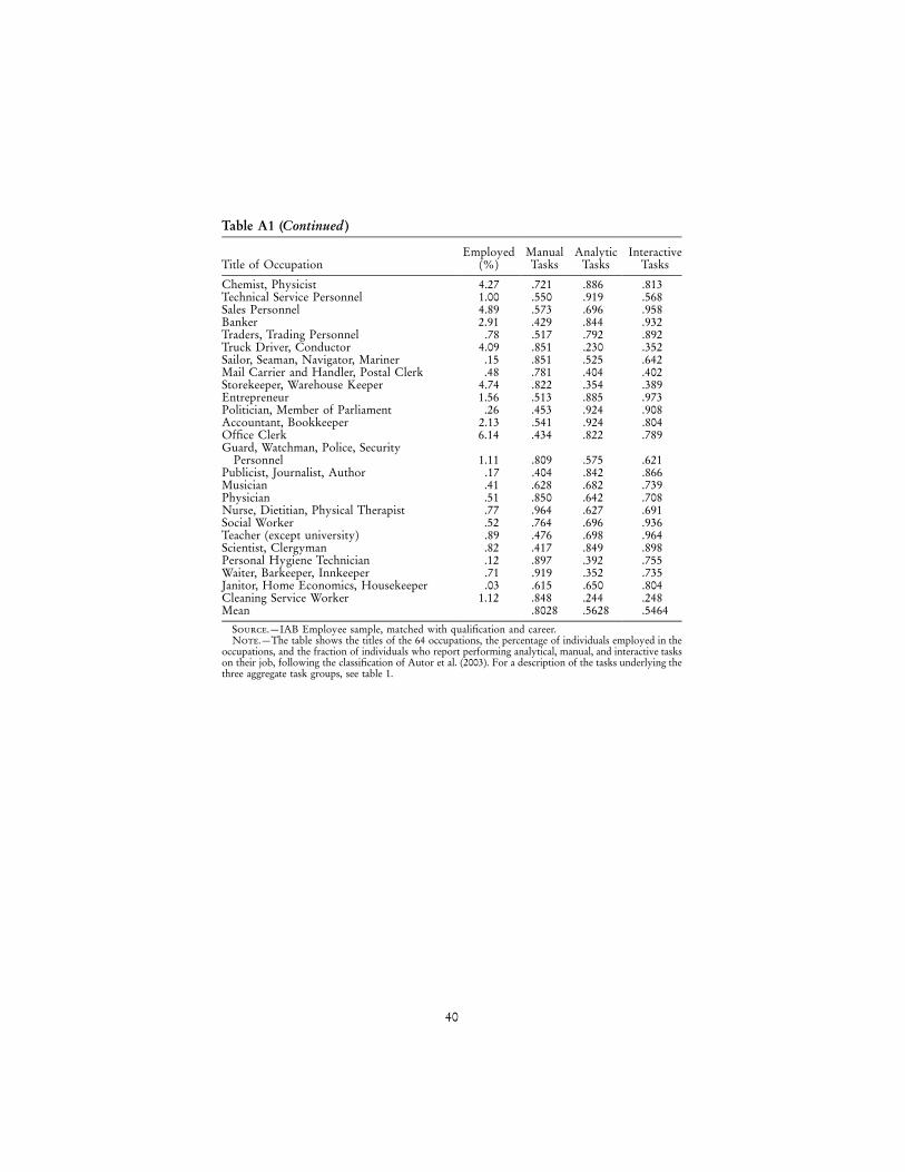
40

Table A1 (Continued)

Title of OccupationEmployed

(%)ManualTasks

AnalyticTasks

InteractiveTasks

Chemist, Physicist 4.27 .721 .886 .813Technical Service Personnel 1.00 .550 .919 .568Sales Personnel 4.89 .573 .696 .958Banker 2.91 .429 .844 .932Traders, Trading Personnel .78 .517 .792 .892Truck Driver, Conductor 4.09 .851 .230 .352Sailor, Seaman, Navigator, Mariner .15 .851 .525 .642Mail Carrier and Handler, Postal Clerk .48 .781 .404 .402Storekeeper, Warehouse Keeper 4.74 .822 .354 .389Entrepreneur 1.56 .513 .885 .973Politician, Member of Parliament .26 .453 .924 .908Accountant, Bookkeeper 2.13 .541 .924 .804Office Clerk 6.14 .434 .822 .789Guard, Watchman, Police, Security

Personnel 1.11 .809 .575 .621Publicist, Journalist, Author .17 .404 .842 .866Musician .41 .628 .682 .739Physician .51 .850 .642 .708Nurse, Dietitian, Physical Therapist .77 .964 .627 .691Social Worker .52 .764 .696 .936Teacher (except university) .89 .476 .698 .964Scientist, Clergyman .82 .417 .849 .898Personal Hygiene Technician .12 .897 .392 .755Waiter, Barkeeper, Innkeeper .71 .919 .352 .735Janitor, Home Economics, Housekeeper .03 .615 .650 .804Cleaning Service Worker 1.12 .848 .244 .248Mean .8028 .5628 .5464

Source.—IAB Employee sample, matched with qualification and career.Note.—The table shows the titles of the 64 occupations, the percentage of individuals employed in the

occupations, and the fraction of individuals who report performing analytical, manual, and interactive taskson their job, following the classification of Autor et al. (2003). For a description of the tasks underlying thethree aggregate task groups, see table 1.

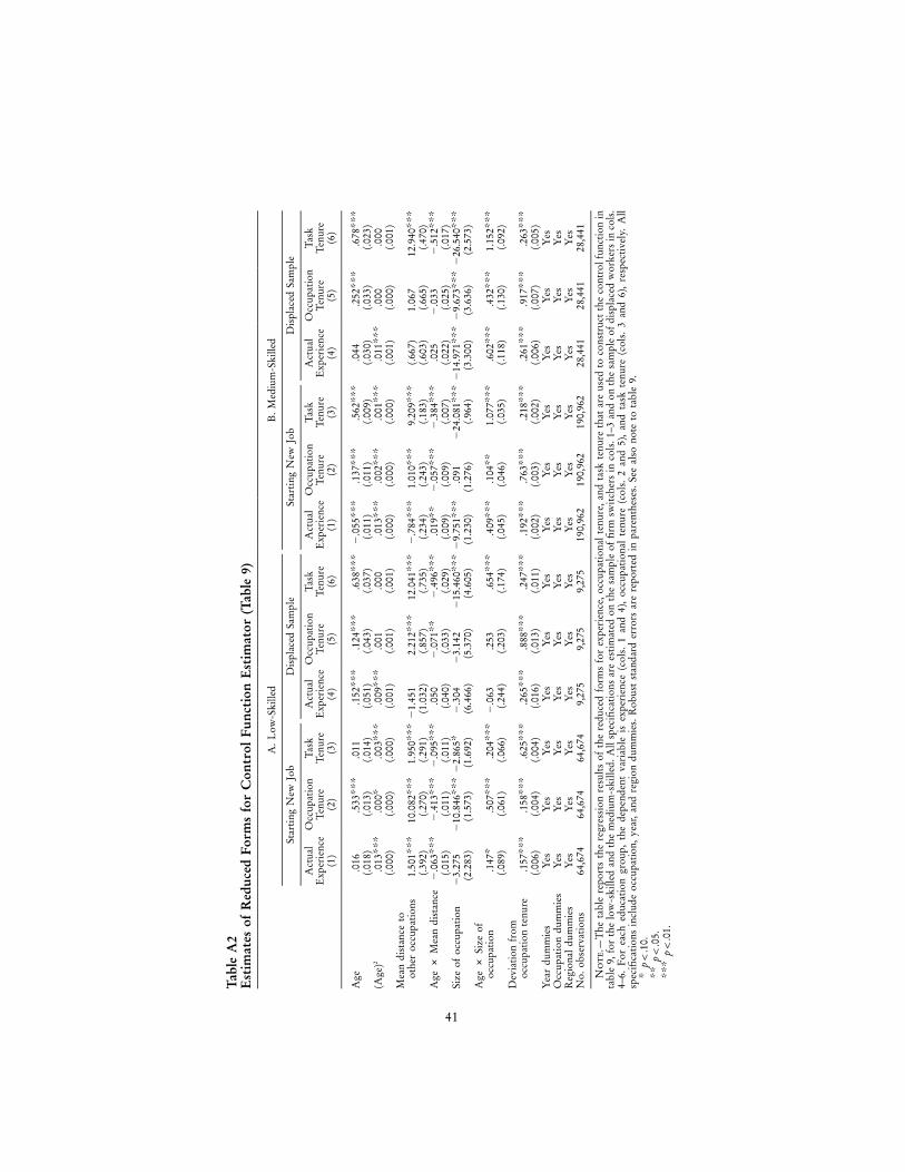
41

Tabl

eA

2E

stim

ates

ofR

educ

edFo

rms

for

Con

trol

Func

tion

Est

imat

or(T

able

9)

A.L

ow-S

kille

dB

.Med

ium

-Ski

lled

Star

ting

New

Job

Dis

plac

edSa

mpl

eSt

artin

gN

ewJo

bD

ispl

aced

Sam

ple

Act

ual

Exp

erie

nce

(1)

Occ

upat

ion

Tenu

re(2

)

Task

Tenu

re(3

)

Act

ual

Exp

erie

nce

(4)

Occ

upat

ion

Tenu

re(5

)

Task

Tenu

re(6

)

Act

ual

Exp

erie

nce

(1)

Occ

upat

ion

Tenu

re(2

)

Task

Tenu

re(3

)

Act

ual

Exp

erie

nce

(4)

Occ

upat

ion

Tenu

re(5

)

Task

Tenu

re(6

)

Age

.016

.533

***

.011

.152

***

.124

***

.638

***

�.0

55**

*.1

37**

*.5

62**

*.0

44.2

52**

*.6

78**

*(.0

18)

(.013

)(.0

14)

(.051

)(.0

43)

(.037

)(.0

11)

(.011

)(.0

09)

(.030

)(.0

33)

(.023

)(A

ge)2

.013

***

.000

*.0

03**

*.0

09**

*.0

01.0

00.0

13**

*.0

02**

*.0

01**

*.0

11**

*.0

00.0

00(.0

00)

(.000

)(.0

00)

(.001

)(.0

01)

(.001

)(.0

00)

(.000

)(.0

00)

(.001

)(.0

00)

(.001

)M

ean

dist

ance

toot

her

occu

patio

ns1.

501 *

**10

.082

***

1.95

0***

�1.

451

2.21

2***

12.0

41**

*�

.784

***

1.01

0***

9.20

9***

(.667

)1.

067

12.9

40**

*(.3

92)

(.270

)(.2

91)

(1.0

32)

(.857

)(.7

35)

(.234

)(.2

43)

(.183

)(.6

03)

(.665

)(.4

70)

Age

#M

ean

dist

ance

�.0

63**

*�

.413

***

�.0

95**

*.0

50�

.071

**�

.496

***

.019

**�

.057

***

�.3

84**

*.0

25�

.033

�.5

12**

*(.0

15)

(.011

)(.0

11)

(.040

)(.0

33)

(.029

)(.0

09)

(.009

)(.0

07)

(.022

)(.0

25)

(.017

)Si

zeof

occu

patio

n�

3.27

5�

10.8

46**

*�

2.86

5*�

.304

�3.

142

�15

.460

***

�9.

751*

**.0

91�

24.0

81**

*�

14.9

71**

*�

9.67

3***

�26

.540

***

(2.2

83)

(1.5

73)

(1.6

92)

(6.4

66)

(5.3

70)

(4.6

05)

(1.2

30)

(1.2

76)

(.964

)(3

.300

)(3

.636

)(2

.573

)A

ge#

Size

ofoc

cupa

tion

.147

*.5

07**

*.2

04**

*�

.063

.253

.654

***

.409

***

.104

**1.

077*

**.6

02**

*.4

32**

*1.

152*

**(.0

89)

(.061

)(.0

66)

(.244

)(.2

03)

(.174

)(.0

45)

(.046

)(.0

35)

(.118

)(.1

30)

(.092

)D

evia

tion

from

occu

patio

nte

nure

.157

***

.158

***

.625

***

.265

***

.888

***

.247

***

.192

***

.763

***

.218

***

.261

***

.917

***

.263

***

(.006

)(.0

04)

(.004

)(.0

16)

(.013

)(.0

11)

(.002

)(.0

03)

(.002

)(.0

06)

(.007

)(.0

05)

Yea

rdu

mm

ies

Yes

Yes

Yes

Yes

Yes

Yes

Yes

Yes

Yes

Yes

Yes

Yes

Occ

upat

ion

dum

mie

sY

esY

esY

esY

esY

esY

esY

esY

esY

esY

esY

esY

esR

egio

nal

dum

mie

sY

esY

esY

esY

esY

esY

esY

esY

esY

esY

esY

esY

esN

o.ob

serv

atio

ns64

,674

64,6

7464

,674

9,27

59,

275

9,27

519

0,96

219

0,96

219

0,96

228

,441

28,4

4128

,441

No

te.—

The

tabl

ere

port

sth

ere

gres

sion

resu

lts

ofth

ere

duce

dfo

rms

for

expe

rien

ce,o

ccup

atio

nal

tenu

re,a

ndta

skte

nure

that

are

used

toco

nstr

uct

the

cont

rolf

unct

ion

inta

ble

9,fo

rth

elo

w-s

kille

dan

dth

em

ediu

m-s

kille

d.A

llsp

ecifi

cati

ons

are

esti

mat

edon

the

sam

ple

offi

rmsw

itch

ers

inco

ls.1

–3an

don

the

sam

ple

ofdi

spla

ced

wor

kers

inco

ls.

4–6.

For

each

educ

atio

ngr

oup,

the

depe

nden

tva

riab

leis

expe

rien

ce(c

ols.

1an

d4)

,oc

cupa

tion

alte

nure

(col

s.2

and

5),

and

task

tenu

re(c

ols.

3an

d6)

,re

spec

tive

ly.

All

spec

ifica

tions

incl

ude

occu

patio

n,ye

ar,a

ndre

gion

dum

mie

s.R

obus

tst

anda

rder

rors

are

repo

rted

inpa

rent

hese

s.Se

eal

sono

teto

tabl

e9.

*p

!.1

0.**

p!

.05.

***

p!

.01.

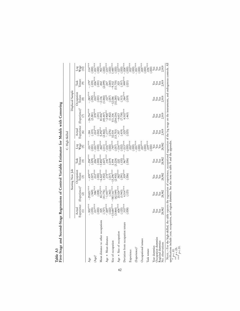
42

Tabl

eA

3Fi

rst-

Stag

ean

dSe

cond

-Sta

geR

egre

ssio

nsof

Con

trol

Var

iabl

eE

stim

ator

for

Mod

els

wit

hC

enso

ring

C.H

igh-

Skill

ed

Star

ting

New

Job

Dis

plac

edSa

mpl

e

Act

ual

Exp

erie

nce

(1)

(Exp

erie

nce)

2

(2)

Occ

upat

ion

Tenu

re(3

)

Task

Tenu

re(4

)

Log

Wag

e(5

)

Act

ual

Exp

erie

nce

(6)

(Exp

erie

nce)

2

(7)

Occ

upat

ion

Tenu

re(8

)

Task

Tenu

re(9

)

Log

Wag

e(1

0)

Age

�.5

02**

*�

29.8

21**

*�

.439

***

�.2

58**

*.1

01**

*�

.184

�26

.754

***

�.2

83**

*�

.179

*.1

14**

*(.0

35)

(.569

)(.0

27)

(.029

)(.0

01)

(.123

)(2

.281

)(.0

92)

(.105

)(.0

00)

(Age

)2.0

17**

*.5

86**

*.0

12**

*.0

06**

*�

.001

***

.014

***

.578

***

.010

***

.006

***

�.0

01**

*(.0

00)

(.008

)(.0

00)

(.000

)(.0

00)

(.002

)(.0

31)

(.001

)(.0

01)

(.000

)M

ean

dist

ance

toot

her

occu

patio

ns.5

2540

.772

***

�6.

422*

**�

3.85

0***

.460

***

5.29

2**

81.8

16*

�2.

136

.842

.901

***

(.727

)(1

1.77

6)(.5

52)

(.607

)(.0

11)

(2.4

60)

(45.

447)

(1.8

40)

(2.0

99)

(.000

)A

ge#

Mea

ndi

stan

ce�

.069

***

�1.

443*

**.1

74**

*.1

46**

*�

.016

***

�.1

77**

�2.

908*

*.1

07*

.047

�.0

33**

*(.0

22)

(.360

)(.0

17)

(.019

)(.0

00)

(.076

)(1

.402

)(.0

57)

(.065

)(.0

00)

Size

ofoc

cupa

tion

�13

.684

***

�58

3.16

1***

�13

.296

***

1.59

4.7

45**

*10

.534

111.

336

�12

.086

�9.

332

1.48

5***

(3.8

64)

(62.

549)

(2.9

30)

(3.2

24)

(.057

)(1

3.75

3)(2

54.0

34)

(10.

285)

(11.

735)

(.000

)A

ge#

Size

ofoc

cupa

tion

.606

***

20.5

24**

*.5

82**

*.0

20�

.016

***

�.3

57�

4.61

3.4

57.3

03�

.027

***

(.120

)(1

.943

)(.0

91)

(.100

)(.0

02)

(.419

)(7

.738

)(.3

13)

(.357

)(.0

00)

Dev

iatio

nfr

omoc

cupa

tion

tenu

re.3

10**

*4.

514*

**.3

09**

*.9

67**

*�

.013

***

.325

***

4.51

0***

.384

***

.999

***

�.0

08**

*(.0

08)

(.123

)(.0

06)

(.006

)(.0

00)

(.025

)(.4

63)

(.019

)(.0

21)

(.000

)E

xper

ienc

e.0

02**

*.0

02**

*(.0

00)

(.000

)(E

xper

ienc

e)2

�.0

01**

*�

.001

***

(.000

)(.0

00)

Occ

upat

iona

lte

nure

.007

***

.005

***

(.000

)(.0

00)

Task

tenu

re.0

39**

*.0

36**

*(.0

00)

(.000

)Y

ear

dum

mie

sY

esY

esY

esY

esY

esY

esY

esY

esY

esY

esO

ccup

atio

ndu

mm

ies

Yes

Yes

Yes

Yes

Yes

Yes

Yes

Yes

Yes

Yes

Reg

iona

ldu

mm

ies

Yes

Yes

Yes

Yes

Yes

Yes

Yes

Yes

Yes

Yes

No.

obse

rvat

ions

28,9

8228

,982

28,9

8228

,982

28,9

822,

919

2,91

92,

919

2,91

92,

919

No

te.—

For

the

high

-ski

lled,

the

tabl

ere

port

sth

ere

gres

sion

ofex

peri

ence

,occ

upat

iona

lreg

ress

ion

ofth

elo

gw

age

onth

ein

stru

men

ts,a

nden

doge

nous

cont

rols

.All

spec

ifica

tions

incl

ude

year

,occ

upat

ion,

and

regi

ondu

mm

ies.

See

also

note

tota

ble

9an

dth

eap

pend

ix.

*p

!.1

0.**

p!

.05.

***

p!

.01.

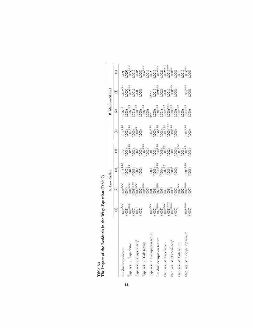
43

Tabl

eA

4T

heIm

pact

ofth

eR

esid

uals

inth

eW

age

Equ

atio

n(T

able

9)

A.L

ow-S

kille

dB

.Med

ium

-Ski

lled

(1)

(2)

(3)

(4)

(1)

(2)

(3)

(4)

Res

idua

lex

peri

ence

�.0

25**

*�

.024

***

�.0

14**

*�

.012

�.0

11**

*�

.006

**�

.007

***

�.0

09(.0

02)

(.004

)(.0

05)

(.008

)(.0

02)

(.003

)(.0

03)

(.005

)E

xp.r

es.#

Exp

erie

nce

.002

***

.004

***

.001

**.0

05**

*.0

03**

*.0

06**

*.0

02**

*.0

05**

*(.0

00)

(.001

)***

(.001

)(.0

02)

(.000

)(.0

01)

(.001

)(.0

01)

Exp

.res

.#(E

xper

ienc

e)2

.000

.000

***

.000

.000

.000

**.0

00**

*.0

00.0

00*

(.000

)(.0

00)

(.000

)(.0

00)

(.000

)(.0

00)

(.000

)(.0

00)

Exp

.res

.#Ta

skte

nure

�.0

05**

*�

.007

***

�.0

06**

*�

.006

***

(.000

)(.0

02)

(.000

)(.0

01)

Exp

.res

.#O

ccup

atio

nte

nure

�.0

02**

*�

.001

.000

.001

�.0

02**

*0*

*0*

**�

.002

(.000

)(.0

01)

(.001

)(.0

01)

(.000

)(.0

00)

(.001

)(.0

01)

Res

idua

loc

cupa

tion

tenu

re.0

66**

*.0

69**

*.0

40**

*.0

40**

*.0

36**

*.0

38**

*.0

29**

*.0

27**

*(.0

02)

(.003

)(.0

04)

(.005

)(.0

01)

(.001

)(.0

02)

(.002

)O

cc.r

es.#

Exp

erie

nce

�.0

02**

*.0

00�

.002

**.0

03**

�.0

01**

*.0

02**

*.0

00.0

02**

*(.0

01)*

**(.0

01)

(.001

)(.0

02)

(.000

)***

(.000

)***

(.001

)(.0

01)*

**O

cc.r

es.#

(Exp

erie

nce)

2.0

00**

*.0

00*

.000

*.0

00.0

00**

*.0

00**

*.0

00**

*.0

00**

(.000

)(.0

00)

(.000

)(.0

00)

(.000

)(.0

00)

(.000

)(.0

00)

Occ

.res

.#Ta

skte

nure

�.0

02**

*�

.003

***

�.0

02**

*�

.001

(.000

)(.0

01)

(.000

)(.0

01)

Occ

.res

.#O

ccup

atio

nte

nure

�.0

03**

*�

.002

***

�.0

03**

*�

.002

**�

.004

***

�.0

03**

*�

.004

***

�.0

03**

*(.0

00)

(.000

)(.0

01)

(.001

)(.0

00)

(.000

)(.0

00)

(.000

)

44

Tabl

eA

4(C

onti

nued

)

A.L

ow-S

kille

dB

.Med

ium

-Ski

lled

(1)

(2)

(3)

(4)

(1)

(2)

(3)

(4)

Res

idua

lta

skte

nure

�.0

06�

.006

�.0

11**

*�

.004

�.0

07(.0

14)

(.004

)(.0

09)

Task

res.

#E

xper

ienc

e.0

01.0

00�

.001

.001

(.001

)(.0

03)

(.001

)(.0

02)

Task

res.

#(E

xper

ienc

e)2

.000

**.0

00*

.000

***

.000

(.000

)(.0

00)

(.000

)(.0

00)

Task

res.

#Ta

skte

nure

�.0

03**

�.0

02*

�.0

01**

�.0

01(.0

01)

(.001

)(.0

00)

(.001

)Ta

skre

s.#

Occ

upat

ion

tenu

re.0

02**

�.0

010*

**�

.002

**(.0

01)

(.001

)(.0

00)

(.001

)p-

valu

efo

rjo

int

sign

ifica

nce

(%)

.00

.00

.00

.00

.00

.00

.00

.00

No

te.—

The

tabl

ere

port

sth

eco

effi

cien

tson

the

resi

dual

san

dth

eir

inte

ract

ion

wit

hth

em

ain

regr

esso

rsto

cont

rolf

orse

lect

ion

inta

ble

9.T

heco

lum

nnu

mbe

rsin

this

tabl

eco

rres

pond

toco

ls.

1–4

inta

ble

9.St

anda

rder

rors

(in

pare

nthe

ses)

are

boot

stra

pped

wit

h10

0re

plic

atio

ns.T

hela

stco

lum

nre

port

sth

ep-

valu

eof

the

test

for

join

tsi

gnifi

canc

eof

the

resi

dual

san

dth

ein

tera

ctio

nte

rms.

See

also

the

note

tota

ble

9.*

p!

.10.

**p

!.0

5.**

*p

!.0

1.


Appendix B

Blundell and Powell (2004) Control Variable Estimator

For the high-skilled, the control variable estimates in table 9, columns3–6, are based on the semiparametric estimator proposed by Blundell andPowell (2004). This estimator accounts for censoring in addition to en-dogenous regressors. It does so, however, at the price of imposing com-mon returns on the observable human capital variables. For simplicity,we drop the subscript The model iso.

ln W p min {X b � u , c },it it it t

where are the endogenous regressors, is the scalar error term, andX uit it

is the time-dependent censoring point. For notational convenience, wect

suppress all exogenous regressors here. The reduced form links the in-struments to the endogenous regressors:Zit

X p Z g � v ,it it it

where is a scalar error term and g is the unknown coefficient vectorvit

with suitable dimensions. Instead of imposing independence between( and , the estimator imposes a weaker conditional quantile ex-u , v ) Zit it it

clusion restriction:

F (qFX , Z ) { Pr {u ≤ qFX , Z }u it it it it it

p Pr {u ≤ qFv } p F (qFv ),it it u it

q � R.

This assumption implies that the dependence of the regressors andXiot

the error term is driven by the residuals (control variable). Tou vit it

consistently estimate the reduced form above, we also require that. The estimation then proceeds as follows. First, we es-E[v FZ ] p 0it it

timate the control variable from regressions of the endogenous re-vit

gressors on the instruments and other control variables. Then, we pre-dict the conditional quantile of from a quantile regression of logˆln Wit

wages on the endogenous regressors, instruments and other control var-iables. The final step involves a weighted least squares regression of allpairwise differences of the predicted dependent variable on theˆln Wit

endogenous regressors . The weights are determined by a multivariateXit


kernel function that is declining in the distance between the residualsand . Formally, the second-stage estimator is defined asˆ ˆv vit it

�1

ˆ ˆv � vis jt ′ˆ ˆ ˆb p K t t (X � X ) (X � X ) #�� v is jt is jt is jt( )[ ]h! !s t i j n

ˆ ˆv � vis jt ′ ˆ ˆˆ ˆK t t(X � X ) (ln W � ln W ) ,�� v is is jt is jt( )[ ]h! !s t i j n

where is the kernel function and is a sequence of scalar bandwidthK (7) hv n

terms; is a “trimming” term, constructed so that unless the estimatedˆ ˆt t p 0is is

quantiles and and fall in some compact set S. We used theˆln W 1 0 X vis is is

product epanechnikov kernel and a separate bandwidth for each endog-hn

enous variable. Standard errors are bootstrapped using 200 replications.

References

Abraham, Katherine G., and Henry S. Farber. 1987. Job duration, seniority,and earnings. American Economic Review 77, no. 3:278–97.

Adda, Jerome, Christian Dustmann, Costas Meghir, and Jean-Marc Robin.2006. Career progression and formal versus on-the-job training. IZADiscussion Paper no. 2260, Institute for the Study of Labor, Bonn.

Altonji, Joseph, and Robert Shakotko. 1987. Do wages rise with jobseniority? Review of Economic Studies 54, no. 3:437–59.

Altonji, Joseph, and Nicholas Williams. 2005. Do wages rise with jobseniority? A reassessment. Industrial and Labor Relations Review 58,no. 3:370–97.

Autor, David, Frank Levy, and Richard J. Murnane. 2003. The skillcontent of recent technological change: An empirical investigation.Quarterly Journal of Economics 118, no. 4:1279–1333.

Becker, Gary S. 1964. Human capital. Chicago: University of Chicago Press.Blundell, Richard, and James Powell. 2004. Censored regression quantiles

with endogenous regressors. Photocopy, Department of Economics,University of California, Berkeley.

Borghans, Lex, Bas der Weel, and Bruce A. Weinberg. 2009. Interpersonalstyles and labor market outcomes. Journal of Human Resources 43:4.

DiNardo, John, and Jorn-Steffen Pischke. 1997. The returns to computeruse revisited: Have pencils changed the wage structure too? QuarterlyJournal of Economics 112, no. 1:291–303.

Dustmann, Christian, and Costas Meghir. 2005. Wages, experience andseniority. Review of Economic Studies 72, no. 1:77–108.

Dustmann, Christian, and Uta Schonberg. 2009. Training and unionwages. Review of Economics and Statistics 91, no. 2:363–76.


Farber, Henry S. 1999. Mobility and stability: The dynamics of job changein labor markets. In Handbook of labor economics, vol. 3, ed. OrleyAshenfelter and David Card. Amsterdam: Elsevier Science.

Fitzenberger, Bernd, and Karsten Kohn. 2005. Gleicher Lohn fur gleicheArbeit? Zum Zusammenhang zwischen Gewerkschaftsmitgliedschaftund Lohnstruktur in Westdeutschland, 1985–1997 [Equal wage forequal work? On the relationship between union membership and thewage structure in West Germany, 1985–97]. Journal for Labour MarketResearch 38, nos. 2/3:125–46.

Fitzenberger, Bernd, and Astrid Kunze. 2005. Vocational training and gen-der: Wages and occupational mobility among young workers. OxfordReview of Economic Policy 21, no. 3:392–415.

Fitzenberger, Bernd, and Alexandra Spitz-Oner. 2004. Die Anatomie desBerufswechsels: Eine empirische Bestandsaufnahme auf Basis der BiBB/IAB, Daten 1998/99 [The anatomy of occupational switches: An em-pirical overview on the basis of the BIBB/IAB data 1998/99]. In Bil-dung, Wirtschaftswissenschaftliches Seminar in Ottobeuren [Education,economic seminar in Ottobeuren], ed. Wolfgang Franz, Hans J. Ramser,and Manfred Stadler, 29–54. Tubingen: Mohr Siebeck.

Flinn, Christopher. 1986. Wages and job mobility of young workers.Journal of Political Economy 94, no. 3:S88–S110.

Florens, Jean-Pierre, James J. Heckman, Costas Meghir, and Ed Vytlacil.2008. Identification of treatment effects using control functions in modelswith continuous, endogenous treatment and heterogeneous effects. Econ-ometrica 76, no. 5:1191–1206.

Gibbons, Robert, and Lawrence F. Katz. 1991. Layoffs and lemons. Journalof Labor Economics 9, no. 4:351–80.

Gibbons, Robert, Lawrence F. Katz, Thomas Lemieux, and Daniel Parent.2005. Comparative advantage, learning, and sectoral wage determination.Journal of Labor Economics 23, no. 1:681–724.

Gibbons, Robert, and Michael Waldman. 2004. Task-specific human capital.American Economic Review 94, no. 2:203–7.

———. 2006. Enriching a theory of wage and promotion dynamics insidefirms. Journal of Labor Economics 24, no. 1:59–107.

Heckman, James J., and Guilherme L. Sedlacek. 1985. Heterogeneity,aggregation, and market wage functions: An empirical model of self-selection in the labor market. Journal of Political Economy 93, no. 6:1077–1125.

Heckman, James J., and Ed Vytlacil. 1998. Instrumental variables methodsfor the correlated random coefficient model. Journal of Human Resources33, no. 4:974–1002.

Honore, Bo. 1992. Trimmed LAD and least squares estimation of trun-cated and censored regression models with fixed effects. Econometrica60, no. 3:533–65.


Ingram, Beth F., and George Neumann. 2006. The returns to skill. LabourEconomics 13, no. 1:35–59.

Jaffe, Adam B. 1986. Technological opportunity and spillovers of R&D:Evidence from firms’ patents, profits, and market value. AmericanEconomic Review 76, no. 5:984–1001.

Jovanovic, Bojan. 1979a. Firm-specific capital and turnover. Journal ofPolitical Economy 87, no. 6:1246–60.

———. 1979b. Job matching and the theory of turnover. Journal ofPolitical Economy 87, no. 5:972–90.

Jovanovic, Bojan, and Yaw Nyarko. 1997. Stepping-stone mobility.Carnegie-Rochester Series of Public Policy 46, no. 1:289–325.

Kambourov, Gueorgui, and Iourii Manovskii. 2009a. Occupational mo-bility and wage inequality. Review of Economic Studies 76, no. 2:731–59.

———. 2009b. Occupational specificity of human capital. InternationalEconomic Review 50, no. 1:63–115.

Kletzer, Lori. 1989. Returns to seniority after permanent job loss.American Economic Review 79, no. 3:536–43.

Lazear, Edward P. 2009. Firm-specific human capital: A skill-weightsapproach. Journal of Political Economy 117, no. 5:914–40.

Ljungqvist, Lars, and Thomas J. Sargent. 1998. The European unem-ployment dilemma. Journal of Political Economy 106, no. 3:514–50.

Malamud, Ofer. 2005. Breadth vs. depth: The effect of academic specializationon labor market outcomes. Harris School Working Paper Series, no. 05.17,Harris Graduate School of Public Policy Studies, University of Chicago.

McCall, Brian P. 1990. Occupational matching: A test of sorts. Journalof Political Economy 98, no. 1:45–69.

Miller, Robert. 1984. Job matching and occupational choice. Journal ofPolitical Economy 92, no. 6:1086–1120.

Mincer, Jacob. 1974. Schooling, experience, and earnings. New York:Columbia University Press.

Neal, Derek. 1995. Industry-specific capital: Evidence from displacedworkers. Journal of Labor Economics 13, no. 4:653–77.

———. 1999. The complexity of job mobility among young men. Journalof Labor Economics 17, no. 2:237–61.

Parent, Daniel. 2000. Industry-specific capital and the wage profile:Evidence from the National Longitudinal Study of Income Dynam-ics. Journal of Labor Economics 18, no. 2:306–23.

Pavan, Ronni. 2005. Career choice and wage growth. Photocopy,Department of Economics, University of Chicago.

Poletaev, Maxim, and Chris Robinson. 2008. Human capital specificity:Evidence from the Dictionary of occupation titles and Displaced WorkerSurveys, 1984–2000. Journal of Labor Economics 26, no. 3:387–420.

Roy, A. D. 1951. Some thoughts on the distribution of earnings. OxfordEconomic Papers 3, no. 2:135–46.


Shaw, Kathryn. 1984. A formulation of the earnings function using theconcept of occupational investment. Journal of Human Resources 19,no. 3:319–40.

———. 1987. Occupational change, employer change, and the transfer-ability of skills. Southern Economic Journal 53, no. 3:702–19.

Spitz-Oner, Alexandra. 2006. Technical change, job tasks, and risingeducational demands: Looking outside the wage structure. Journal ofLabor Economics 24, no. 2:235–70.

Topel, Robert. 1991. Specific capital, mobility, and wages: Wages rise withjob seniority. Journal of Political Economy 99, no. 1:145–76.

Topel, Robert, and Michael Ward. 1992. Job mobility and the careers ofyoung men. Quarterly Journal of Economics 107, no. 2:439–80.

Violante, Gianluca L. 2002. Technological acceleration, skill transferability,and the rise in residual inequality. Quarterly Journal of Economics 117,no. 1:297–338.

Wasmer, Etienne. 2004. Interpreting Europe and U.S. labor market dif-ferences: The specificity of human capital investments. American Eco-nomic Review 96:811–31.

Yamaguchi, Shintaro. 2008. Career progression and comparative advantage.Photocopy, Department of Economics, McMaster University.

How General Is Human Capital? A Task-Based...

Documents

Transcript of How General Is Human Capital? A Task-Based...