How Exporters Grow - · PDF fileHow Exporters Grow Doireann Fitzgeraldy Stefanie Hallerz Yaniv...

How Exporters Grow∗

Doireann Fitzgerald† Stefanie Haller‡ Yaniv Yedid-Levi§

August 2017¶

Abstract

We use customs microdata to distinguish between competing models of demand and

customer base. We purge supply-side variation from the data by comparing quantities

and prices across markets within a firm. Higher quantities on entry forecast survival

in an export market, but survival is unrelated to initial prices. Conditioning on sur-

vival, there is economically and statistically significant growth of quantities within a

firm-market, but no dynamics of prices. These facts are consistent with a model of

the demand side of firm growth where entrants to a market learn about idiosyncratic

demand through quantities, generating selective exit, while survivors grow by accumu-

lating customer base through marketing and advertising. They present a challenge to

models where firms learn about idiosyncratic demand through prices, and to models

where current demand depends on lagged sales.

∗Online appendix available at www.doireann.com. This work makes use of data from the Central StatisticsOffice, Ireland, which is CSO copyright. The possibility for controlled access to confidential micro data setson the premises of the CSO is provided for in the Statistics Act 1993. The use of CSO data in this workdoes not imply the endorsement of the CSO in relation to the interpretation or analysis of the data. Thiswork uses research data sets that may not exactly reproduce statistical aggregates published by the CSO.We thank the staff of the CSO for making this project possible. Expert research assistance was provided byAdrian Corcoran, Matt Shapiro and Anthony Priolo. Doireann Fitzgerald is grateful for financial supportfrom the NSF under grant number 0647850. Yaniv Yedid-Levi is grateful for financial support from theSocial Sciences and Humanities Research Council of Canada. We thank Costas Arkolakis, Kim Ruhl, JamesTybout, Daniel Xu, and participants in the 2015 and 2016 NBER Summer Institute for comments andsuggestions. The views expressed herein are those of the authors and not necessarily those of the FederalReserve Bank of Minneapolis or the Federal Reserve System.†Federal Reserve Bank of Minneapolis and NBER, [email protected]‡School of Economics, University College Dublin, [email protected]§Vancouver School of Economics, University of British Columbia, [email protected]¶First draft: July 2015.

1

1 Introduction

Recent research makes demand and customer base central to the analysis of firm dynamics,

business cycles, and international trade.1 Although much has been learned, there is as yet no

consensus on how best to model the mechanisms through which firms’ demand and customer

base grow. As a result, three different models are actively used in the literature. This state

of affairs is unsatisfactory, as answers to several key questions differ across models. In this

paper, we use customs microdata for Ireland to provide evidence on this issue. We show

that the behavior of prices is inconsistent with two of the models commonly used. We also

structurally estimate a simple model with idiosyncratic demand and customer base which is

qualitatively and quantitatively consistent with the behavior of both quantities and prices,

thus providing a foundation on which the literature can build.

The three distinct approaches to modeling demand and customer base we refer to are as

follows: (1) Firms learn from prices about their idiosyncratic demand in a market, leading

to selection and sales growth, as firms exit markets with low demand while in markets with

high demand they reduce markups to slide down their demand curves; (2) Demand depends

on lagged sales, so firms expand in a market by first charging markups below their steady

state level to shift out demand, then gradually increasing their markups as sales rise; (3)

Demand depends on customer base, which firms acquire through non-price activities such as

marketing and advertising.

These models differ in their predictions about certain moments of prices. Model (1) im-

plies that conditioning on supply-side factors (such as marginal cost, quality, etc.), higher

initial prices in a market should forecast survival. In addition, conditioning on survival as

well as supply-side factors, growth in quantities in a market subsequent to entry should be

accompanied by declining prices. Model (2) implies that conditioning on survival as well as

supply-side factors, growth in quantities in a market subsequent to entry should be accom-

panied by increasing prices. Model (3) implies that as long as expenditure on marketing

and advertising shifts demand, but does not affect its price elasticity, then conditional on

both supply-side factors and survival, growth in quantities in a market subsequent to entry

is possible without any price dynamics.

Customs microdata provide a very convenient environment within which to examine

these predictions. This is because we observe quantities and prices, and can purge supply-

1See, among others, Arkolakis (2016), Arkolakis et al. (2017), Drozd and Nosal (2012a,b) Eaton et al.(2011), Eaton et al. (2014), Foster et al. (2008, 2016), Gilchrist et al. (2017), Gourio and Rudanko (2014),Ravn et al. (2006), Ruhl and Willis (2016).

2

side variation from the data under the twin assumptions that (a) demand is log-linear in

the components of supply and demand that are common across markets, and (b) supply

side factors do not vary across export markets within a firm and a product. We implement

this by looking only at residual variation in quantities and prices after conditioning on firm-

product-year fixed effects.

Conditional on these fixed effects, and on a set of fixed effects to control for market-

specific factors that are common to all firms, we find that higher quantities in the year of

entry to a market forecast longer survival in that market. In contrast, survival is unrelated to

prices in the year of entry. Meanwhile, conditioning on survival, there are economically and

statistically significant dynamics of quantities, but no dynamics of prices within a given firm,

product, and market. In particular, in export spells which last at least 7 years, quantities

grow on average more than 50% between the second and sixth year in a market, but this

growth is accompanied by a zero average change in prices. We also find (as others have done),

that the probability of exit is decreasing with age in a market. We perform a comprehensive

set of robustness checks to confirm these facts. They hold across a range of manufacturing

industries, across different export markets, and across firms of different size and ownership.

The behavior of prices that we document is clearly inconsistent with models (1) and

(2).2 But both price and quantity facts are consistent with model (3). This suggests that

marketing and advertising is important for acquiring and retaining customers, consistent

with the substantial fraction of GDP that is devoted to these expenditures.3 We do not have

data on marketing and advertising expenditures for our firms, but to demonstrate clearly the

role they play, we structurally estimate a model of customer accumulation through marketing

and advertising that can match all the quantity and price facts.

The model we estimate has the following features. We assume that entrants to a market

must learn about market-specific idiosyncratic demand. But in contrast to model (1), we

assume that firms set prices rather than quantities in the face of uncertainty about demand.

They then learn through observing quantities whether their demand in a market is perma-

nently high, or permanently low. Due to fixed costs of market participation, this generates

selective exit from markets where firms learn through low initial quantities that they have

low demand. Meanwhile, in markets where firms learn through high initial quantities that

they have high idiosyncratic demand, they find it optimal to invest and grow by accumulat-

2In addition, the behavior of prices is inconsistent with a “quality” (supply-side) explanation for within-market quantity growth, as this would imply that higher marginal cost, and hence higher prices, shouldaccompany growth in quantities.

3Arkolakis (2010) notes that marketing and advertising expenditures may account for up to 8% of GDP.

3

ing customer base through marketing and advertising. Assuming that demand is isoelastic

in prices, and that customer base shifts demand, but does not change the price elasticity of

demand, markups are flat as quantity grows. In addition to the elements just described, we

also allow learning to be slow (i.e. slower than Bayesian learning), and we allow for both

irreversibility and quadratic costs of adjusting investment in customer base.

We estimate this model by simulated method of moments. We target the quantity and

exit moments from the data, since price moments are matched by construction. The model

fits all moments remarkably well. It matches the relationship between initial quantities and

survival; the growth of quantities in short and long export episodes; and the behavior of the

exit hazard. By shutting down the elements of the model one-by-one, we show that it is

indeed minimal, in the sense that all elements are necessary to match the facts. To match

the quantity and exit moments quantitatively, there must be nontrivial costs of adjusting

investment in customer base, and learning about idiosyncratic demand must be much slower

than if firms were Bayesian.

To our knowledge, our paper is the first to use a comprehensive set of quantity and

price moments to distinguish between competing models of demand and customer base.

However we are not alone in investigating price dynamics. A series of recent papers document

price moments using manufacturing census and customs data: some claim that prices are

increasing with plant age or tenure in an export market, while others claim that they are

decreasing.4 These claims are at odds with each other, and with our findings. We investigate

the source of the differences between these results and ours by estimating the specifications

used by these papers in our data. In contrast to our approach, these papers either mix

supply-side with demand-side variation, or fail to separate selection from true dynamics, or

both. We can replicate the results of these papers in our data. This suggests that purging

supply-side variation and controlling for selection are both important in order to understand

of what is going on on the demand side.

Models with demand and customer base are applied to a wide range of important issues.

For example, Arkolakis et al. (2017) use model (1) to argue that firm entry may be ineffi-

ciently low due to learning about demand. Meanwhile, Foster et al. (2008, 2016) point to

model (2) and argue that revenue-based TFP measures may systematically underestimate

the contribution of entrants to productivity growth, because entrants have lower markups.

Ravn et al. (2006) use model (2) to support a theory of business cycles with countercyclical

4This includes Foster et al. (2008) who use plant census data for the US, and Bastos et al. (2017),Berman et al. (2015) and Piveteau (2016) who use customs data for Portugal and France. Foster et al. andPiveteau claim prices are increasing, while Bastos et al. and Berman et al. claim they are drecreasing.

4

markups, while Hall (2014) points out that countercyclical markups are difficult to reconcile

with the procyclicality of advertising. Drozd and Nosal (2012b) investigate the performance

of model (2) in matching international business cycle comovements, and find it does poorly.

Gourio and Rudanko develop a hybrid of models (2) and (3) to show that sluggish adjust-

ment of customer base has important implications for firm responses to shocks, and for the

relationship between investment and Tobin’s Q. Our findings therefore have applications in

several fields, and provide a foundation upon which a wide range of future research can build.

The paper is organized as follows. In the second section, we describe our data. In the third

section, we describe our empirical strategy. In the fourth section, we describe our results on

quantity, price, and exit moments. In the fifth section, we show that these moments allow us

to distinguish between different models of demand and customer base. In the sixth section,

we lay out our model. In the seventh section, we describe how we structurally estimate our

model, and report our estimation results. In the eighth section, we report the results of some

simulation exercises illustrating the quantitative importance of adjustment costs. The final

section concludes.

2 Data description

We make use of two sources of confidential micro data made available to us by the Central

Statistics Office (CSO) in Ireland: the Irish Census of Industrial Production (CIP) and Irish

customs records. Here, we note the key points about each data set. The data are described in

detail in the online appendix; the appendix also describes a third data set (the PRODCOM

survey), which we use to obtain the number of products produced at the firm level and

firm-product prices used in robustness checks.

2.1 Census of Industrial Production

The CIP is an annual census of manufacturing, mining, and utilities. Firms with three

or more persons engaged are required to file returns.5 We make use of data for the years

1996-2009 and for NACE Revision 1.1 sectors 10-40 (manufacturing, mining, and utilities).

Of the variables collected in the CIP, those we make use of in this paper are total revenue,

employment, the country of ownership, and an indicator for whether the firm has multiple

plants in Ireland.

5Multiplant firms also fill in returns at the level of individual plants. We work with the firm-level data,since this is the level at which the match with customs records can be performed.

5

In constructing our sample for analysis, we drop firms with a zero value for total revenue

or zero employees in more than half of their years in the sample. We perform some recoding

of firm identifiers to maintain the panel dimension of the data, for example, in cases in which

ownership changes.

2.2 Customs records

Our second source of data is customs records of Irish merchandise exports for the years 1996-

2014. The value (euros) and quantity (tonnes)6 of exports are available at the level of the

VAT number, the Combined Nomenclature (CN) eight-digit product, and the destination

market (country), aggregated to an annual frequency. These data are matched by the CSO

to CIP firms using a correspondence between VAT numbers and CIP firm identifiers, along

with other confidential information. The online appendix provides additional information

on this match.

A key feature of customs in the European Union is that data for intra-EU and extra-EU

trade are collected separately, using two different systems called Intrastat and Extrastat.

The threshold for mandatory reporting of intra-EU exports (635,000 euro per year in total

shipments within the EU) is different from the threshold for extra-EU exports (254 euro per

transaction).7 The high threshold for intra-EU exports likely leads to censoring of exports

by small exporters to the EU. However it applies not at the market level, but to exports to

the EU as a whole, and we observe many firms exporting amounts below the 635,000 euro

threshold to individual EU markets.

An important feature of the customs data is that the eight-digit CN classification system

changes every year. We concord the product-level data over time at the most disaggregated

level possible following the approach of Pierce and Schott (2012) and Van Beveren et al.

(2012). For our baseline analysis, we restrict attention to the period 1996-2009, for which

we have CIP data in addition to customs data, and for this analysis we make use only of

customs data that matches to a CIP firm. In some robustness checks, we make use of the

full sample period, 1996-2014. When we do so, we do not condition on a CIP match. We

perform the product concordance separately for the two different sample periods, as dictated

by the Pierce and Schott approach.

As a result, we have annual data on value and quantity of exports at the firm-product-

market level, where the product is defined at the eight-digit (concorded) level, and the

6The value is always available, but the quantity is missing for about 10% of export records.7Intra-EU exports below the threshold are recovered based on VAT returns. The destination market

within the EU is not recorded for these returns.

6

Table 1: Summary statistics: Firms and exports, averages 1996-2009Mean number of firms per year 4748Mean employees 50Mean age (years) 17Share of firms foreign owned 0.12Share of multi-plant firms 0.03Mean number of concorded products per firm 4Share of firms exporting 0.44Exporter size premium (employees, mean) 1.65Exporter size premium (revenue, mean) 1.85Mean export share conditional on exporting 0.32Mean number of markets per exporter 6.6

Notes: Statistics are for our cleaned data set of CIP firms. Firms are defined as exporters if they are matched to positiveconcorded product exports from customs data. Export intensity is calculated as total concorded product exports from customsdivided by sales reported in the CIP. Values greater than 1 are replaced by 1. Source: CSO and authors’ calculations.

Table 2: Summary statistics: percentage of exporters by change in number of markets yearto year

Change <-6 -5 -4 -3 -2 -1 0 1 2 3 4 5 >6% 2 1 2 3 5 11 51 12 5 3 2 1 3

Notes: Statistics are for our cleaned data set of CIP firms. Firms are defined as exporters if they are matched to positiveconcorded product exports from customs data. Export revenue is concorded product export revenue from customs data. Thereare 140 export markets. Source: CSO and authors’ calculations.

market refers to the destination country. We use this to construct a price (unit value) by

dividing value by quantity, where available. In aggregate trade statistics, unit value data at

the product level are notoriously noisy. However, conditioning on the exporting firm as well

as the product considerably reduces this noise.

2.3 Summary statistics

Table 1 shows summary statistics on the firms in our data, focusing in particular on export-

ing behavior. Export participation is high, export intensity conditional on participation is

high, and at least half of exporters participate in multiple markets (we observe 140 distinct

export markets over the course of the panel). These facts are typical of small open European

economies (see ISGEP (2008)). Apart from the relatively high rate of export participation

and the high intensity of exporting conditional on participation, the broad facts about ex-

porting are also similar to those documented for large developed countries such as the United

States and France and for developing countries such as Colombia.

7

Entry and exit are not synchronized across different export markets within a given firm.8

This is illustrated in Table 2, which reports summary statistics on churn in the number of

export markets from year to year. In any given year, on average 49% of exporters change

the number of markets they participate in. This is a lower bound on churn, as some firms

may keep the total number of export markets constant, while switching between markets.

This churn induces within-firm-year variation in market tenure and completed export spell

length, which we exploit in our empirical strategy.

3 Empirical strategy

The goal of our empirical analysis is to characterize moments of the data that can discrimi-

nate between competing models of demand and customer base. There are two key elements

to our strategy: (1) we purge quantities and prices of variation due to supply-side factors,

and (2), we separate variation that is due to selection from variation that is due to dynam-

ics. In addition, we control for market-specific variation that is common across all firms.

We focus throughout on conditional means, as these moments are sufficient to distinguish

between models.

We purge the data of variation due to supply-side factors and that component of demand

that is common across markets by focusing on moments of the data conditional on firm-

product-year fixed effects. This controls for supply and the common component of demand

under two assumptions. First, the marginal cost of production must be the same across all

markets for a given firm, product, and year. Second, since we express quantities and prices

in logs, demand must be log-linear in own price and in the common demand component.9

The issue with respect to selection is as follows. Suppose there is selection on idiosyn-

cratic demand, i.e. firms systematically exit markets with low demand earlier than markets

with high demand. Then if we pool across all export episodes, we will find an increasing

relationship between exports and time since entry, even if there are no dynamics whatso-

ever within any given export episode. We deal with this issue by differentiating between

export episodes according to how long they last. We then examine how initial conditions

forecast survival, and also document dynamics conditioning on the ex-post duration of the

export episode. This gives us information on the nature of selection, while also isolating true

dynamics. This extends the approach of Ruhl and Willis (2016) to documenting exporter

8This is consistent with Lawless (2009), who uses a different data set on Irish firms.9Log-linearity is required for our strategy to purge supply-side factors from quantities, but is not required

for our strategy to work for prices.

8

dynamics, and has some similarities with the approach of Altonji and Shakotko (1987) to

dealing with selection in estimating the effect of job tenure on wages.

We use Table 3 to explain the intuition for our approach. The top panel gives a (fictitious)

example of the pattern of participation of a firm-product pair in markets A through G over a

period of six years. We define an export spell as a continuous episode of market participation,

i.e. an episode in which there are positive exports in every year. Table 3 shows one export

spell in all markets except market E, where there are two distinct export spells under our

definition.

In the second panel, we show how we construct a variable we call market tenure. We set

market tenure equal to 1 in the first year a firm exports a given product to a given market

after not exporting in the previous period. Tenure is incremented by 1 in each subsequent

year of continuous participation. If the firm-product exits a market for some period, market

tenure is reset to 1 in the first subsequent year of participation (e.g., market E in year 4).

Note that we do not observe market tenure if entry is censored (e.g., markets A and G in

Table 3).

The third panel shows how we construct a variable we call spell length. If an export spell

is neither left- nor right-censored, we observe completed spell length (markets B, C, D, E).

If we observe zero exports for one or more years after some positive exports, any reentry is

counted as part of a distinct export spell (e.g., market E).10 The fourth panel shows that by

top-coding spell length at some number, we can assign a spell length to some right-censored

spells (e.g., market F, where completed spell length is at least 3).

As Table 3 illustrates, there can be cross-sectional variation in both spell length and

market tenure within a firm-product-year. By comparing initial conditions in spells which

start in the same year, but have different completed market tenure (e.g. comparing markets

B, D, and E in year 2) we can learn about the nature of selection on market-specific demand.

By further examining how outcomes vary with market tenure within spells of a given length

(e.g. markets B, C and F), we can separate true dynamics from the effect of selection. Our

baseline strategy exploits two types of variation to identify dynamics: variation in market

tenure over time within a given export spell, and variation in market tenure across spells of

a given length within a firm-product-year.11

10In our baseline analysis we treat these “reentry” spells the same as “first entry” spells. In robustnesschecks, we relax this and treat them differently.

11One potential concern with this latter dimension of variation is that it may confound selection in thetiming of entry with dynamics. In robustness checks, we deal with this issue by adding firm-product-cohortfixed effects, or by expressing all outcomes relative to the outcome in the year of entry. Our findings arerobust to these modifications.

9

Table 3: Illustration of identifying variation in market tenure and spell lengthYear 1 2 3 4 5 6Market I. ParticipationA X X X X X XB X X XC X X XD X XE X XF X X XG XMarket II. Market tenureA cens cens cens cens cens censB 1 2 3C 1 2 3D 1 2E 1 1F 1 2 3G censMarket III. Spell lengthA cens cens cens cens cens censB 3 3 3C 3 3 3D 2 2E 1 1F cens cens censG censMarket IV. Spell length, topcoded at 3A cens cens cens cens cens censB 3 3 3C 3 3 3D 2 2E 1 1F 3 3 3G cens

10

3.1 Product revenue, quantity, price, and product-market exit

Mechanically, we implement our strategy as follows. Let wijkt be log revenue, log quantity, or

log price. Let δk be a market dummy variable (our baseline results are robust to including

market-year or product-market-year fixed effects). Let cijt be a firm-product-year fixed effect

that controls for marginal cost. Let aijkt be a vector of indicator variables for firm i’s tenure

in market k with product j. Let sijkt be a vector of indicators for the length of the relevant

spell. This indicator does not vary within a spell, but is indexed by t to capture the fact that

we may observe multiple export spells of different length for firm i, product j, and market k

over the period of our panel (e.g., market E in Table 3). We top-code both market tenure and

spell length at seven years in our baseline specification. We drop spells whose length is right-

censored at a level below the top-code.12 Let censijk be an indicator for spells that are both

left- and right-censored. Including these spells helps control for firm-product-year-specific

factors. We then estimate:

wijkt = δk + cijt + β′(aijkt ⊗ sijkt

)+ censijk + εijkt . (1)

The symbol ⊗ indicates the Kronecker product. We do not observe tenures of greater than

s for a spell that lasts s years, so the redundant interactions are dropped.

The vector β contains the coefficients of interest. Appropriate linear combinations of the

elements of β allow us to characterize variation in initial log revenue, quantity, and price with

completed spell length, and the evolution of log revenue, quantity, and price with market

tenure over the lifetime of spells of different length.

To characterize the distribution of spell lengths, our second empirical exercise examines

the hazard of exit. We adopt a similar strategy to the above to show how the average

probability of exit varies with market tenure, exploiting again only variation within a firm-

product-year to control for supply-side factors. Let X ijkt be an indicator for participation of

firm i with product j in market k at date t. We then estimate the linear probability model:

Pr[X ijkt+1 = 0|X ijk

t = 1]

= δk + cijt + β′aijkt + εijkt . (2)

The terms δk, cijt and aijkt are as above, and β is again the vector of coefficients of interest.

Linearity is clearly less defensible for exit than log-linearity for revenue, quantity and price.

12Allowing the full range of market tenures and spell lengths would force us to drop all right-censoredspells, would not allow us to separately identify the impact of market tenure and spell length for the longestspells, and would also confound cohort effects with the impact of these variables. Using our full panel ofcustoms data, which lasts for 19 years, we show that our key results are robust to top-coding at 10 years.

11

But our estimates do not purport to be structural. All that we ask is that they characterize

average behavior in a way that is informative for distinguishing between models.

3.2 Market revenue, number of products, and market exit

At the firm-market level, we observe revenue and the number of products a firm sells to a

destination. This allows us to characterize the extent to which overall revenue dynamics

depend on dynamics in the number of products.

The construction of market tenure and spell length at the firm-market level is analogous

to the approach at the firm-product-market level. Let wikt be log revenue or log number of

products. Let δk be a market dummy variable. Let cit be a firm-year fixed effect. Let aikt be a

vector of indicator variables for firm i’s tenure in market k. Let sikt be a vector of indicators

for the total length of the relevant spell. Let censik be an indicator for spells that are both

left- and right-censored. We then estimate:

wikt = δk + cit + β′(aikt ⊗ sikt

)+ censik + εikt . (3)

Appropriate linear combinations of the elements of β allow us to characterize variation

in initial revenue and number of products with completed spell length, and the evolution of

log revenue and number of products with market tenure over the lifetime of spells of different

length.

We also characterize the distribution of spell lengths at the firm-market level. Let X ikt

be an indicator for participation of firm i in market k at date t. We then estimate:

Pr[X ikt+1 = 0|X ik

t = 1]

= δk + cit + β′aikt + εikt . (4)

4 Empirical findings

4.1 Product revenue, quantity, price, and product-market exit

The first three columns of Table 4 report results for the baseline estimation of equation

(1), with log revenue, log quantity, and log price in turn as the dependent variable.13 The

omitted category in all regressions is export spells which last exactly one year. The log of

13Table A.5 in the online appendix compares summary statistics on the firm-years included in this analysiswith summary statistics for all firm-years in our data. Exporters included in the analysis are bigger, moreexport-intensive, and export to more destinations than the average exporter.

12

Figure 1: Firm-product-market revenue by completed spell length and market tenure

05

10

15

Ra

tio

of

reve

nu

e t

o 1

−yr

sp

ell

reve

nu

e

0 1 2 3 4 5 6Years in market

1 2

3 4

5 6

7

Notes: Figure shows evolution of revenue at the firm-product-market level with market tenure, allowing trajectories to differ byexport spell length. Trajectories are conditional on firm-product-year and market effects. 95% confidence intervals are plotted.Source: CSO and authors’ calculations.

the dependent variable for each of these spells is hence normalized to 0. In the table, we

organize our results into initial values conditional on spell length and within-spell trajectories

normalizing the start of each spell to 0. Figures 1, 2, and 3, graph the trajectories of revenues,

quantities and prices implied by taking the exponential of the relevant sums of coefficients

from Table 4.14

We have four key findings on quantities and prices: (1) Higher initial quantities predict

longer export spells. For spells lasting between one and four years, all pairwise comparisons

of initial quantities are statistically different. (2) Initial prices do not predict export spell

length. (3) Quantities grow dramatically in the first five years of export spells that last

at least seven years. This growth is statistically significant up to a horizon of four years

and is not driven purely by part-year effects in the first year (i.e. there is economically and

statistically significant growth between years 2 and 4). (4) Within successful export spells,

up to a horizon of six years, there are no statistically or economically significant dynamics

14We graph the standard errors for all revenue and quantity trajectories, but for price trajectories, wegraph only the standard errors on the longest spell to make the figure easier to read. None of the points onthe price trajectories are significantly different from 1.

13

Table 4: Dynamics of revenue, quantity, price, and number of productsObs. level Firm-product-market Firm-market

Dep. var. (ln) Revenue Quantity Price Revenue # Products

Spell lgth Spell intercept

2 years 0.51 (0.02)** 0.52 (0.02)** -0.01 (0.01) 0.40 (0.04)** 0.10 (0.01)**

3 years 0.76 (0.03)** 0.76 (0.04)** 0.00 (0.02) 0.74 (0.06)** 0.15 (0.01)**

4 years 0.95 (0.05)** 0.95 (0.05)** 0.00 (0.02) 0.84 (0.07)** 0.18 (0.02)**

5 years 1.07 (0.06)** 1.08 (0.07)** -0.01 (0.03) 1.09 (0.09)** 0.19 (0.02)**

6 years 1.13 (0.08)** 1.09 (0.08)** 0.04 (0.03) 1.15 (0.11)** 0.25 (0.03)**

7+ years 1.39 (0.05)** 1.39 (0.05)** 0.01 (0.02) 1.32 (0.05)** 0.28 (0.01)**

cens 3.66 (0.03)** 3.70 (0.03)** -0.04 (0.01)** 3.98 (0.03)** 0.91 (0.01)**

Mkt tenure 2-year spell

2 years -0.03 (0.03) -0.03 (0.03) 0.00 (0.02) -0.02 (0.05) -0.00 (0.01)


2 years 0.44 (0.04)** 0.45 (0.05)** -0.01 (0.02) 0.48 (0.07)** 0.11 (0.02)**

3 years -0.05 (0.05) -0.05 (0.05) 0.00 (0.02) 0.02 (0.07) 0.01 (0.02)


2 years 0.53 (0.06)** 0.55 (0.06)** -0.02 (0.03) 0.61 (0.09)** 0.13 (0.02)**

3 years 0.55 (0.06)** 0.60 (0.06)** -0.05 (0.03)* 0.57 (0.09)** 0.12 (0.02)**

4 years -0.02 (0.07) -0.01 (0.07) -0.01 (0.03) 0.19 (0.10)* 0.01 (0.02)


2 years 0.63 (0.09)** 0.62 (0.09)** 0.01 (0.04) 0.71 (0.12)** 0.16 (0.03)**

3 years 0.70 (0.09)** 0.69 (0.09)** 0.01 (0.04) 0.74 (0.12)** 0.19 (0.03)**

4 years 0.57 (0.09)** 0.61 (0.09)** -0.04 (0.04) 0.59 (0.12)** 0.19 (0.03)**

5 years -0.01 (0.09) 0.01 (0.09) -0.02 (0.04) 0.05 (0.12) 0.05 (0.03)


2 years 0.74 (0.11)** 0.78 (0.11)** -0.04 (0.05) 0.68 (0.14)** 0.21 (0.04)**

3 years 0.87 (0.11)** 0.95 (0.11)** -0.07 (0.05) 0.90 (0.14)** 0.21 (0.04)**

4 years 0.85 (0.11)** 0.92 (0.11)** -0.07 (0.05) 1.03 (0.14)** 0.24 (0.04)**

5 years 0.71 (0.11)** 0.75 (0.11)** -0.04 (0.05) 0.75 (0.14)** 0.14 (0.04)**

6 years 0.12 (0.11) 0.14 (0.11) -0.02 (0.05) 0.11 (0.15) 0.00 (0.04)

Mkt tenure 7+ year spell

2 years 0.85 (0.06)** 0.88 (0.06)** -0.03 (0.03) 1.01 (0.07)** 0.21 (0.02)**

3 years 1.16 (0.06)** 1.20 (0.06)** -0.03 (0.03) 1.35 (0.07)** 0.28 (0.02)**

4 years 1.31 (0.06)** 1.34 (0.06)** -0.03 (0.03) 1.51 (0.07)** 0.32 (0.02)**

5 years 1.34 (0.06)** 1.37 (0.06)** -0.04 (0.03) 1.60 (0.07)** 0.33 (0.02)**

6 years 1.30 (0.06)** 1.33 (0.07)** -0.03 (0.03) 1.59 (0.07)** 0.32 (0.02)**

7+ years 1.28 (0.06)** 1.35 (0.06)** -0.07 (0.03)** 1.64 (0.06)** 0.33 (0.02)**

Fixed effects

Firm-prod-yr Yes Yes Yes No No

Firm-yr No No No Yes Yes

Market Yes Yes Yes Yes Yes

N 312952 312952 312952 113912 113912

rsq 0.76 0.82 0.90 0.65 0.56

rsq-adj 0.58 0.69 0.82 0.58 0.47

Notes: In the first column, the sample is restricted to firm-product-market-years for which quantity data are available. Depen-dent variable is in turn log revenue, log quantity, and log unit value at the firm-product-market-year level, and log revenue andlog number of products at the firm-market-year level. Full set of firm-product-year and market effects included in firm-product-market-year regressions. Full set of firm-year and market effects included in firm-market-year regressions. Omitted categoryis spells that last one year. Robust standard errors calculated. ** significant at 5%, * significant at 10%. Source: CSO andauthors’ calculations.

14

Figure 2: Firm-product-market quantity by completed spell length and market tenure

05

10

15

Ra

tio

of

qu

an

tity

to

1−

yr

sp

ell

qu

an

tity


1 2

3 4

5 6

7

Notes: Figure shows evolution of quantities at the firm-product-market level with market tenure, allowing trajectories to differby export spell length. Trajectories are conditional on firm-product-year and market effects. 95% confidence intervals areplotted. Source: CSO and authors’ calculations.

Figure 3: Firm-product-market price by completed spell length and market tenure, differentscale

0.2

.4.6

.81

1.2

Ra

tio

of

price

to

1−

yr

sp

ell

price


1 2

3 4

5 6

7

Notes: Figure shows evolution of prices at the firm-product-market level with market tenure, allowing trajectories to differ byexport spell length. Trajectories are conditional on firm-product-year and market effects. 95% confidence interval for spells of7+ years is plotted. Source: CSO and authors’ calculations.

15

Table 5: Exit hazardMarket tenure Firm-prod-mkt Firm-mkt

2 years -0.13 (0.00)** -0.16 (0.00)**3 years -0.20 (0.00)** -0.22 (0.01)**4 years -0.24 (0.00)** -0.25 (0.01)**5 years -0.25 (0.01)** -0.27 (0.01)**6 years -0.24 (0.01)** -0.27 (0.01)**

7+ years -0.24 (0.00)** -0.26 (0.01)**Fixed effects

Firm-prod-yr Yes NoFirm-yr No YesMarket Yes Yes

N 381452 103297rsq 0.70 0.47

rsq-adj 0.47 0.34

Notes: Dependent variable is an indicator for exit in the next period. Full set of firm-product-year and market effects includedat the firm-product-market-year level. Full set of firm-year and market effects included at the firm-market-year level. Omittedcategory is market tenure equal to one year. Robust standard errors calculated. ** significant at 5%, * significant at 10%.Source: CSO and authors’ calculations.

in prices.

The first column of Table 5 reports results for the baseline estimation of the firm-product-

market exit equation, i.e. equation (2). Figure 4 illustrates these findings. The probability

of exit is initially decreasing in market tenure and then flattens out after four years in a

market.

4.2 Market revenue, number of products, and market exit

The fourth and fifth columns of Table 4 report the results from the baseline estimation

of equation (3), with log revenue and log number of products as the dependent variable

in turn.15 These results are illustrated in Figures 5 and 6. The evolution of revenue at

the firm-market level is qualitatively very similar to the evolution of revenue at the firm-

product-market level, though the trajectories are somewhat steeper, reflecting the fact that

the number of products per market also evolves with market tenure. Focusing on the longest

spells, 70-80% of the growth of revenue at the market level along the growth path is accounted

for by within-product growth in revenue,16 indicating that the within-product margin is of

15Note that the sample of firms included in columns 4 and 5 includes some firms not present in column1, as the revenue equation at the product level drops the 10% of observations for which quantity is notavailable.

16This is consistent with the findings of Hottman et al. (2016) on the importance of of the productextensive margin.

16

Figure 4: Exit probability and market tenure: Firm-product-market and firm-market

−.3

−.2

−.1

0C

ha

ng

e in

exit p

rob

ab

ility

re

lative

to

ye

ar

1

0 1 2 3 4 5 6Market tenure

Firm−market Firm−product−market

Notes: Figure shows reduction in probability of exit at the firm-market and firm-product-market levels with compared toprobability of exit in the first year in a market. Trajectories are conditional on firm-year and market and firm-product-yearand market effects, respectively. 95% confidence intervals are plotted. Source: CSO and authors’ calculations.

first-order importance in explaining export growth.

The second column of Table 5 reports the results from the baseline estimation of the

firm-market exit equation (4). Figure 4 illustrates the evolution of the probability of exit

with market tenure at the market level, with the corresponding evolution at the product-

market level for comparison. The evolution of exit at the market level is very similar to the

evolution of exit at the product-market level, though the probability of exit continues falling

until the firm is five years in the market.17

4.3 Robustness

We make extensive checks of both specification robustness and robustness to various cuts of

the data. We describe key findings here, and refer to specific tables in the online appendix

where the full set of results (including some not described here) is reported.

17The unconditional probability of exit in the first year is substantially higher at the firm-product-marketlevel than at the firm-market level (62% vs. 45%).

17

Figure 5: Firm-market revenue by completed spell length and market tenure

05

10

15

20

Ra

tio

of

reve

nu

e t

o 1

−yr

sp

ell

reve

nu

e


1 2

3 4

5 6

7

Notes: Figure shows evolution of revenue at the firm-market level with market tenure, allowing trajectories to differ by exportspell length. Trajectories are conditional on firm-year and market effects. Source: CSO and authors’ calculations.

Figure 6: Number of products per market by completed spell length and market tenure

.51

1.5

2R

atio

of

#p

rod

to

1−

yr

sp

ell

#p

rod


1 2

3 4

5 6

7

Notes: Figure shows evolution of number of products at the firm-market level with market tenure, allowing trajectories to differby export spell length. Trajectories are conditional on firm-year and market effects. Source: CSO and authors’ calculations.

18

4.3.1 Specification robustness

Our results are qualitatively and quantitatively almost unchanged when we include market-

year fixed effects (Tables A.6 and A.7 and Figures A.4, A.5 and A.6) or product-market-year

fixed effects (Tables A.8 and A.9 and Figures A.6, A.7 and A.8) as appropriate.

We restrict our analysis to the subsample of products and firms for which a second

measure of quantity (other than tonnes) is reported, constructing quantities and unit values

using this alternative measure (Table A.10 and Figures A.9 and A.10). For this subsample,

which is 1/6 of the baseline sample, we find that lower initial prices predict that export spells

last longer than one year. However, all other results are unchanged.

We vary the level at which spell lengths and market tenure are top-coded, in the range

5 to 8 in our 14-year baseline sample, and in the range 7 to 10 in the 19-year sample that

does not require a match between a firm in the customs data and a firm in the Census of

Industrial Production. The key results are qualitatively unchanged (a subset of these results

are reported in the appendix in Tables A.11 through A.17 and Figures A.11 through A.16).

However, there is some evidence that prices drop below their initial levels in the later years

of the longest export spells (10+ years in duration). This is at a point when there are no

longer any dynamics in quantities.

One concern about our baseline specification is that there may be some dimension of

idiosyncratic demand that is observable to firms, but not to us, and firms may choose to enter

markets that are more attractive along this dimension earlier than less attractive markets.

Since we make use of cross sectional variation in market tenure in spells of the same length to

identify dynamics, this kind of selection in the timing of entry could lead us to infer within-

spell growth in quantities where there is none. To address this, we estimate two alternative

specifications. First we augment the baseline specification with firm-product-cohort fixed

effects (Tables A.18 and A.19 and Figures A.17, A.18 and A.19). Second, we normalize the

dependent variable by the value in the first year of the relevant spell (Table A.20 and Figures

A.20 and A.21). The first approach allows us to estimate differences in initial quantities and

prices across spells of different length, while the second does not. We find that the growth of

quantities in the longest spells is marginally lower under these specifications, but otherwise

our findings are both qualitatively and quantitatively unchanged.

4.3.2 First and subsequent markets, products and spells

Prompted by the possibility of a role for learning about demand in explaining post-entry

export dynamics, several papers use micro data on exports to examine the difference in dy-

19

namics between “firsts” (first markets, first products, first spells) and “subsequents” (sub-

sequent markets, subsequent products, subsequent spells). We perform similar cuts of our

data.

We allow trajectories to differ across export spells based on the number of markets the

firm exported to at the beginning of the spell: a total of three or fewer markets versus four or

more markets (Tables A.21, A.22 and A.23 and Figures A.22, A.23 and A.24). Identification

of the coefficients of interest comes from within-firm-product-year or within-firm-market-year

variation across markets, so restricting to the case where there are few markets reduces the

precision of the estimates. However, the key stylized facts are qualitatively replicated for

both sets of spells. The one statistically significant difference is that the probability of exit

falls more with market tenure in first markets than in subsequent markets.

We allow trajectories to differ between first products and subsequent products, where a

product is “first” if on entry, the firm does not export any other products to that market,

and is “subsequent” if on entry, the firm already exports at least one product to that market

(Tables A.24, A.25 and A.26 and Figures A.25, A.26 and A.27). The key stylized facts are

qualitatively replicated for both sets of spells. Quantitatively, the only difference is that

in successful spells, the growth of quantities is somewhat steeper for first products than

subsequent products.

We allow trajectories to differ between first spells in a firm-product-market and subse-

quent or reentry spells in the same firm-product-market (Tables A.27, A.28 and A.29 and

Figures A.28, A.29 and A.30). The estimates for subsequent spells are noisy, as there are

relatively few of these spells. However, the key stylized facts are qualitatively replicated for

both sets of spells. The only statistically significant difference is that the probability of exit

in year 1 is lower (by about 7%) in subsequent spells than in first spells.

4.3.3 Firm and product characteristics

We also examine robustness to splitting the sample by firm and product characteristics. We

first estimate separate trajectories for domestic-owned and foreign-owned firms (Tables A.30,

A.31, A.32 and A.33 and Figures A.31, A.32 and A.33). Although they account for only

10% of firms in the CIP, more than half of the observations in our baseline sample come

from foreign-owned firms, as they are bigger and more export-oriented than domestic-owned

firms. The key stylized facts are qualitatively replicated for both sets of firms. The only

statistically significant difference is that growth in quantities in the initial years of successful

export spells is higher in foreign-owned than in domestic-owned firms.

20

We estimate different trajectories based on firm size (as measured by employment) at the

time of firm-product-market or firm-market entry (Tables A.34 through A.42 and Figures

A.34 through A.42). The key stylized facts are qualitatively replicated for small and large

firms. The only difference is that growth in quantities in the initial years of successful

export spells is higher in large than small firms. This does not depend on the threshold for

classifying a firm as large.

We estimate separate sets of trajectories for different industry groups: consumer food

products; consumer nonfood nondurables; consumer durables; intermediates and capital

goods (Tables A.43 through A.52 and Figures A.43, A.44 and A.45). This categorization is

based on the NACE Revision 1.1 three-digit sector of the firm.18 Estimates for consumer

nonfood nondurables and consumer durables are noisy, as there are relatively few firms in

these industries.19 The key stylized facts are qualitatively replicated for all industry groups.

We use a concordance between the Rauch (1999) classification of goods as homogeneous,

reference-priced, or differentiated, and the HS six-digit product classification, to apply the

Rauch classification at the product level in our data. This allows us to classify products for

89% of our baseline estimation sample. Of these, about 5% are classified as homogeneous,

16% as reference-priced, and the remainder as differentiated. We then estimate separate sets

of trajectories for the three groups of products (Tables A.53 through A.58 and Figures A.46,

A.47 and A.48). The key stylized facts are qualitatively replicated for all product types.

4.4 Relation to the empirical literature

There are now two issues to resolve. First, is Ireland special, and are our results driven

by some special feature of the Irish data? Second, how do our findings relate to a series of

conflicting claims about price dynamics in the related literature?

To show that the Irish data is not unusual, we note that we can replicate the findings of

a large body of literature working with firm and customs micro data for other countries. As

mentioned above, summary statistics on the cross-sectional dimension of exporting in our

data are in line with those for other small open European economies. Our findings on the

post-entry dynamics of revenues and exit are similar to those in the previous literature, (e.g.,

Eaton et al. (2008), Eaton et al. (2014), Ruhl and Willis (2016)). Using our data, we can

also replicate a number of facts about the behavior of prices (or more precisely, unit values)

in customs data for other countries. In Fitzgerald et al. (2017), we show that the degree

18The assignment of three-digit sectors to industry groups is detailed in the online appendix.19Pharmaceuticals, a key industry for Ireland in terms of export value, though not employment, is cate-

gorized as a consumer nonfood nondurable.

21

of pricing-to-market in our data is very similar to that for other countries (e.g. France, as

shown by Berman et al. (2012)). In the online appendix to this paper (Table A.63), we show

that prices vary with destination market characteristics just as in the literature surveyed in

Harrigan et al. (2015).

However, our findings on the absence of price dynamics contrast with those in a number

of related papers that claim to show evidence of price dynamics. Using customs data for

France, Berman et al. (2015) claim that prices are decreasing with tenure in a market.20

Bastos et al. (2017) use Portuguese customs data, and also claim that prices are decreasing

with tenure. Piveteau (2016) uses French customs data, and claims that prices are increasing

with tenure in a market.21 Foster et al. (2008) use manufacturing census data on plants in

a narrow set of commodity-like sectors, and also claim an increasing relationship between

prices and plant age.

These contrasting results may be due to the fact that these authors work with empirical

specifications which are different from each other, as well as from our specification. There are

two key points of difference: (1) the treatment of supply-side variation, and (2) the approach

to separating selection from dynamics. In our baseline specification, we purge the data of

variation that is due to supply-side factors by looking at price moments conditional on firm-

product-year fixed effects. While Berman et al. purge the data of supply-side variation using

a similar approach to ours, Bastos et al., Piveteau, and Foster et al. mix supply-side and

demand-side variation in their baseline specifications. As regards selection, in our baseline

specification, we condition on survival to be able to separate true within-firm-product-market

dynamics from selection on prices. While Piveteau also conditions on survival in his baseline

specification, Berman et al., Bastos et al. and Foster et al. do not.

To investigate the hypothesis that the differences between the different sets of results are

driven by specification differences, we estimate the Berman et al. and Piveteau specifications

in our customs data, and a specification that resembles that of Foster et al. using PRODCOM

data at the firm-product level. The results from these exercises are consistent with the

findings of these various authors. When we estimate the Berman et al. specification, we

find a negative (though not significant) relationship between prices and tenure (Table A.64).

When we estimate the Piveteau specification, we find a positive (though not significant)

relationship between prices and tenure (Table A.65).22 When we estimate the Foster et al.

20Berman et al.’s point estimates are very similar to ours, but their standard errors are smaller.21Unlike us, Bastos et al., Berman et al., and Piveteau do not investigate the relationship between initial

prices and survival.22Moreover, in robustness analysis, Berman et al. and Piveteau both estimate specifications that resemble

one of our robustness analyses (Table A.20). In these exercises, they find that prices are flat with respect to

22

specification using PRODCOM data, we find that prices are significantly higher in firms that

have been selling a product for some years than in firms that have just started selling the

same product (Table A.66).

We suspect that the empirical treatment of both supply-side variation and selection

matters because selection and dynamics on the supply side are associated with quite different

price behavior from selection and dynamics on the demand side. This hypothesis is supported

by the fact that when we estimate the Foster et al. specification, we find (as they do) that

lower prices forecast exit. This contrasts sharply with the fact that prices do not forecast

survival when we purge supply-side variation from the data. It is also supported by the fact

that the Berman et al. specification yields results that are quite close to ours despite not

separating selection from dynamics, as their approach purges supply-side variation from the

data.

5 What our findings say about models of demand

As noted in the introduction, there are several alternative approaches to modeling demand

and customer base in the literature on macroeconomics and international trade. We now

compare the predictions of the most prominent of these models with our evidence about the

behavior of quantities and prices. To do this it will be useful to have some notation. Let

firm i’s demand in market k at time t be given by23

Qikt = d

(P ikt , ε

ikt , D

ikt

). (5)

Qikt is the quantity firm i sells in market k at date t. P ik

t is the price the firm charges to

buyers from k. εikt is a shock, idiosyncratic to the firm and the market, which shifts demand

conditional on price. It is exogenous to the firm. Dikt is a variable that is firm- and market-

specific, and which shifts demand conditional on price, but which depends on actions taken

by the firm at t or in previous periods. We refer to it as “customer base.”

market tenure.23For the purpose of illustration, we abstract from the product dimension, and from factors such as

aggregate demand and the aggregate price level in market k that are controlled for by market, market-year,or product-market-year fixed effects in our regressions.

23

5.1 Learning from prices

This model is used in the literature on firm dynamics, and in the literature on international

trade.24 In this model, there is no endogenous component to idiosyncratic demand: Dikt = 0.

Both selection and dynamics result from the fact that idiosyncratic demand εikt has some

persistent component, and is unobserved before firms choose market participation or other

actions. By participating in a market, firms can update the information they use to form

expectations about future idiosyncratic demand. Crucially, in the face of uncertainty about

εikt , firms are assumed to set quantities, and learn by observing realized prices. As a result,

in markets where εikt is high, high prices are observed after entry, and firms infer that the

probability of having high demand in those markets in the future is high. They respond

optimally by increasing quantities, thereby driving prices down as they move along their

demand curve.25 In contrast, in markets where εikt is low, post-entry prices are low. Firms

infer that the probability of having high demand in the future is low. In the presence of

fixed costs of participating in a market, low prices thus lead to early exit.

To sum up, in this model, high initial prices forecast survival, while low initial prices

forecast early exit. Meanwhile, in successful episodes of market participation (i.e. episodes

where exit is not observed), on average prices fall as quantities rise, with the relationship

between quantities and prices being governed by the price elasticity of demand.26 Both of

these predictions are inconsistent with what we find in the data. Robustly, we find that initial

prices do not forecast survival, while initial quantities do. Moreover, in our baseline results,

conditional on survival, there are no statistically or econonomically significant dynamics in

prices.

The fact that in the data, quantities, not prices, forecast survival suggests that firms

may indeed face uncertainty about idiosyncratic demand, but that in the face of uncertainty,

they set prices rather than quantities. This case has not received much attention in the

literature, possibly because it cannot explain growth in quantities: If firms set prices, in

markets with high idiosyncratic demand, they observe high initial quantities, learn thereby

that future demand will be high, and find it optimal to (weakly) raise prices and reduce

quantities sold in response. Only in the limiting case of isoelastic demand, where desired

markups do not depend on beliefs about future demand, are there are no dynamics of either

prices or quantities.

24See Arkolakis et al. (2017), Bastos et al. (2017) and Berman et al. (2015).25Firms do not anticipate price dynamics, but there are dynamics in realized prices because of dynamics

in beliefs.26We show this formally in section 3 of the online appendix.

24

5.2 Current demand depends on lagged sales

This model has generated some interest in the literature on business cycles.27 It has also

been used in the literature on firm dynamics and international trade.28 In this model,

customer base Dikt is increasing in lagged sales in the market, i.e. P ik

t−1Qikt−1. This generates

a tradeoff between maximizing profits today, and maximizing profits tomorrow. Firms with

below-steady-state sales in a market expand in that market by first charging low markups

to generate high sales. Demand shifts out as a result, and as sales converge to their steady

state, markups are gradually increased. So according to this model, increasing quantities

should be accompanied by increasing markups. While it is straightforward to allow for

idiosyncratic demand εikt and selection due to fixed costs of market participation in this

model, without taking a stand on how sales on entry to a market are determined (i.e. Dikt

when P ikt−1Q

ikt−1 = 0), the model is silent on whether initial quantities or prices should forecast

survival.

The prediction that increasing markups accompany increasing quantities is clearly incon-

sistent with what we find in the data. In our baseline results, conditional on survival there

are no statistically or econonomically significant dynamics in prices.

5.3 Customer base is acquired through marketing and advertising

This model is used in the literature on international trade29 and business cycles.30 In this

model, demand depends on market-specific customer base Dikt , and firms can acquire cus-

tomer base through non-price activities such as marketing and advertising in the relevant

market. Dynamics can be introduced by assuming that customer base can be accumulated

(i.e. Dikt is increasing in Dik

t−1), and investment in customer base is subject to adjustment

costs. In the formulations generally used in the literature, customer base does not affect the

price elasticity of demand. As a result, by engaging in marketing and advertising, firms can

shift demand and increase quantities without having any impact on optimal markups. It is

straightforward to allow for idiosyncratic demand, εikt , and selection in this model. Firms

want to accumulate higher customer base Dikt in markets with high idiosyncratic demand

εikt . Depending on what firms know about idiosyncratic demand on entry, this can gener-

ate a positive relationship between initial quantities and subsequent quantity growth, as we

27See e.g. Ravn et al. (2006), Gilchrist et al. (2017), and Gourio and Rudanko (2014).28See Foster et al. (2016) and Piveteau (2016).29See Arkolakis (2010, 2016), Eaton et al. (2011), and Eaton et al. (2014).30See Drozd and Nosal (2012a) and Gourio and Rudanko (2014).

25

explore in the next section.

The predictions of this model - under the assumption that customer base does not affect

the price elasticity of demand - are consistent with our finding that there are statistically

and economically significant dynamics of quantities that are not accompanied by dynamics

in prices. We do not have direct evidence of the role of marketing and advertising in within-

market growth. We do not even have data on expenditures on marketing and advertising at

the firm level. But we can certainly infer from the fact that a non-trivial share of GDP is

devoted to marketing and advertising that firms think these activities are valuable for the

bottom line.

5.4 Quality

Finally, in a model where firms tailor quality to the market, dynamics in quality could

generate market-specific dynamics in quantities.31 But such a model would predict that

higher quantities should be accompanied by higher prices, since quality is costly to produce.

This is inconsistent with the joint behavior of quantities and prices in our data. This does not

lead us to reject the idea that quality heterogeneity is important. Rather, we do not think

there is much evidence that within-firm market-specific quality heterogeneity can explain

our results. Across firms, quality heterogeneity may play a key role.

6 A model of market-specific demand

To demonstrate clearly the role of marketing and advertising, we now build the simplest

possible model of the demand side which can match quantity, price, and exit moments. It

is straightforward to build more a more complicated model to match even more moments,

but for our purposes, this would obscure rather than clarify the key mechanisms. The model

can be summarized as follows: Entry is random. Entrants to a market set prices, and

learn through quantities about idiosyncratic demand, generating selective exit. Meanwhile,

survivors grow by accumulating customer base through non-price actions such as marketing

and advertising. Both idiosyncratic demand and customer base shift total demand, but do

not affect the price elasticity of demand, so desired markups are constant. In addition to

these basic elements, for quantitative purposes, we also allow learning to be slow (i.e. slower

than Bayesian learning), and we allow for both irreversibility and quadratic costs of adjusting

31By “quality” we mean something which both increases costs of production, and shifts demand conditionalon price.

26

investment in customer base.32

We model a single-product firm, where the only channel through which decisions across

different markets are interdependent is through a common marginal cost of production. Firm

i is characterized by marginal cost Cit , the same in all markets. The firm observes Ci

t before

making any decisions at date t, and knows the process from which marginal cost is drawn.

As illustrated by Table 2, entry is not perfectly synchronized across markets within the

firm. Moreover, there is a good deal of steady state churn in the number of markets a firm

participates in. This suggests an idiosyncratic dimension to entry and exit at the firm-market

level. To capture this in the simplest possible way, we assume that firm i faces stochastic

sunk costs (Sikt ) and per-period fixed costs (F ikt ) of participating in market k at date t. The

firm observes these costs before deciding to participate at date t, and knows the distributions

from which they are drawn.

Demand for firm i in market k depends on its own price P ikt , on customer base Dik

t , and

on idiosyncratic demand εikt . Demand takes the form:33

Qikt =

(P ikt

)−θ (Dikt

)αexp

(εikt). (6)

Note that neither idiosyncratic demand nor customer base affect the price elasticity of de-

mand (θ). If α ∈ (0, 1), demand is increasing in customer base, but at a diminishing rate.

In this case there is a finite positive steady state for Dikt .

Customer base accumulates as follows:

Dikt = (1− δ)X ik

t−1Dikt−1 + Aikt , (7)

where X ikt ∈ {0, 1} is an indicator for participation in market k by firm i at date t, Aikt is

investment in customer base, and δ is the depreciation rate of customer base.34 Investment

32It is possible to construct an alternative rationalization of the facts based on a price-taking firm thatfaces marginal costs of distributing goods that are increasing in the quantity sold. This explanation has avery similar flavor to the one we pursue.

33We abstract from factors such as aggregate demand and the aggregate price level in market k, as theseare cleaned out of our target moments.

34Full depreciation of customer base on exit is assumed purely for computational tractability.

27

in customer base is subject to both convex costs of adjustment, and irreversibility:

c(Dikt , A

ikt

)=

Aikt + φ

(AiktDikt− δ)2

Dikt if Aikt > 0

0 otherwise.

(8)

This portion of the model resembles Arkolakis (2010), with the modification that customer

base can be accumulated. The irreversibility assumption is very natural in the context of

investment in an intangible such as customer base.

When making choices at date t with respect to market k, firm i does not observe εikt . But

by participating, it may acquire information it can use to condition its future expectations

of idiosyncratic demand. In the face of uncertainty about εikt , it matters whether the firm

sets prices or quantities. We assume that it sets prices. Because demand is CES and there

are no strategic interactions with other firms, the optimal price is equal to the statically

optimal markup over marginal cost ( θθ−1

), irrespective of the firm’s participation history,

information set, realization of εikt , or customer base. In this sense, the model hardwires in

both the orthogonality of initial prices and survival, and a flat path of prices with respect

to market tenure (all of these conditional on marginal cost Cit).

To describe our model of learning, we must specify a process for idiosyncratic demand.

We assume that idiosyncratic demand has two components, permanent and transitory:

εikt = νik + ηikt ,

with

νik ∼ N(0, σ2

ν

)ηikt = ρηikt−1 + ζ ikt

ζ ikt ∼ N(0, σ2

η

)We assume that firm i may be “uninformed” (N ik

t−1 = 0) or “informed” (N ikt−1 = 1) about

market k on entry to period t. An uninformed firm knows only the unconditional distribution

of εikt . An informed firm observes{νik, ηikt−1

}. Potential entrants are always uninformed.

Uninformed participants become informed with probability γ at the end of each period of

participation. Conditional on continued participation, being informed is an absorbing state.

On exiting a market, the firm (whether informed or uninformed), loses its draw of{νik, ηikt−1

},

28

and knows that it will have to redraw from the unconditional distribution if it decides to

participate again in the future.35 As a result, information I ikt about idiosyncratic demand

evolves as follows:

I ikt =

{νik, ηikt−1

}if{X ikt−1 = 1, N ik

t−1 = 1}

∅ if{X ikt−1 = 0

}or{X ikt−1 = 1, N ik

t−1 = 0}.

(9)

This way of modeling information acquisition is both computationally tractable and

flexible, in that it allows the average speed of learning to be fast (γ close to 1) or slow (γ

close to 0), independent of the parameters of the idiosyncratic demand process. In contrast,

under Bayesian learning, where the firm infers εikt−1 by observing quantities sold in period

t − 1 (I ikt ={εikt−1, ε

ikt−2, . . .

}), the speed of learning is determined by the parameters of

the idiosyncratic demand process. Under reasonable parameter values Bayesian learning is

typically very fast, in the sense that the firm need only see one realization of εikt−1 in order for

the conditional expectation of νik to be very close to the true value.36 So we see our model

of learning as a tractable approximation to a model where firms are Bayesian, but only pay

attention to I ikt ={εikt−1, ε

ikt−2, . . .

}with probability γ.

Assuming that firms discount the future at rate β, we can write the intertemporal opti-

mization problem as follows:

V(Dikt−1, X

ikt−1, N

ikt−1, I

ikt , F

ikt , S

ikt , C

it

)=

max

X ikt ∈ {0, 1}Aikt

X ikt

(θ−1)θ−1

θθ(Ci

t)1−θ (

Dikt

)α E (exp(νik + ηikt

)|I ikt)

−X ikt

(F ikt +

(1−X ik

t−1

)Sikt)− c

(Dikt , A

ikt

)+βE

(V(Dikt , X

ikt , N

ikt , I

ikt+1, F

ikt+1, S

ikt+1, C

it

)|I ikt)

(10)

subject to the accumulation equation for customer base, (7), the cost of investment, (8), and

the updating of information, (9), which includes the process for N ikt as a function of lagged

participation.

35This latter assumption is made purely for computational tractability.36This is the case when we estimate our model with Bayesian learning.

29

7 Model estimation and results

7.1 Estimation

In order to estimate the model, we must make some assumptions about the processes for

marginal costs (Cit), sunk costs (Sikt ), and fixed costs (F ik

t ). Because the demand side is our

focus, and all of our target moments are based on demand-side variation alone, we abstract

from supply-side heterogeneity, and set Cit = 1. Given this, we can assume very simple

processes for Sikt and F ikt . With probability λ, independent across firms, markets, and over

time, Sikt = 0, and entry is possible.37 With probability 1− λ, the sunk cost is infinity, and

entry is not possible. With probability 1 − ω, independent across firms, markets, and over

time, F ikt = F <∞, and the firm may choose to participate. With probability ω, the fixed

cost is equal to infinity, and the firm must exit (or remain out of the market).38

We use simulated method of moments to estimate the model. Given values for parameters

β, α, δ, φ, θ, σ2ν , ρ, σ2

η, F , ω, S, λ, and γ, we discretize both exogenous and endogenous

states39 and use value function iteration to solve for the optimal policies for participation

and investment. Using the model parameters and the corresponding optimal policies, we

then simulate post-entry trajectories for 50,000 “firm-markets.” To account for the fact that

there are part-year effects in the data, the length of a period in our model is 6 months. We

stagger entry across 6-month periods, and aggregate up to an annual frequency to construct

the equivalents of the moments we estimate in Section 4. The goal of our estimation is to

choose the vector of parameters that best matches these moments.

We match moments of four types. The first three sets of moments are based on our

estimates conditional on firm-product-year and market fixed effects: the ratios of initial

quantities across spells of different length; the evolution of quantities with market tenure

within spells of different length; and the evolution of exit probabilities with market tenure.

The fourth moment is the average exit rate in the first year in a market across all export

spells in our data for which entry is not censored. We do not target moments related to

prices, as they are matched automatically in our baseline model. The full set of 32 targeted

moments is reported in column (1) of Table 6.

We first preset some parameters not identified by our target moments. Since we calibrate

37In the absence of cost heterogeneity, and under the assumption that all potential entrants have the sameprior about idiosyncratic demand, the assumption that S = 0 is without loss of generality.

38Given a suitable set of target moments, it would be very straightforward to introduce richer processeshere.

39We use three states each for the permanent and transitory idiosyncratic demand shocks (ν and η). Thenumber of endogenous states depends on parameter values.

30

to a 6-month period, we set β = 1.05−0.5. In our baseline model, θ and φ are not separately

identified by our target moments. We pick θ = 2 as a baseline value for θ. This is consistent

with a markup over marginal cost (which does not include fixed costs of production or costs

related to marketing and advertising) of 100%.40 The export entry rate in our model is equal

to λ (1− ω). The average entry rate for non-participants across the 56 export markets that

account for 99% of exports is 1%, so we set λ = 0.01/ (1− ω).

This leaves us with nine parameters,{α, δ, φ, σ2

ν , ρ, σ2η, F, ω, γ

}. We choose these param-

eters to minimize the criterion function m′V m, where m is the difference between the data

moments and the equivalent moments in the model, and V is a diagonal matrix, with the

inverse of the standard deviation of the estimates of the data moments on the diagonal (we

do not include the entry rate in this matrix, as we hit this target by construction). We use

a combination of a particle swarm algorithm and the simplex method to optimize over the

parameter vector.

7.2 Baseline results

The first column of Table 6 reports the data moments. The second column reports the

corresponding fitted values of the moments. Figures 7 and 8 illustrate the fit of the model

by graphing target and fitted moments for quantities and exit. The estimated model matches

all of the key facts in the data. It generates dispersion in initial quantities that is positively

correlated with spell length and of the right order of magnitude, quantities that increase

with market tenure in successful spells as in the data, and an exit hazard that declines

substantially between the first and second year in a market and continues to fall until about

five years in the market, closely matching the data.

In the first row of Table 7, we report the estimated parameters of the baseline model, and

an overall measure of fit based on the criterion function.41 Our estimate of α, the elasticity of

sales with respect to customer base, is 0.50. This indicates that there is a significant role for

customer base in explaining post-entry export dynamics. This customer base depreciates at

a relatively rapid rate: our estimate of δ, 0.46, implies an annual rate of depreciation of 70%,

which is in line with what is found in the empirical literature on advertising summarized in

40The online appendix describes results based on alternative values for θ in Tables A.70 and A.71.41Standard errors are constructed using the method suggested by Gourieroux et al. (1993), as described

in the online appendix. They are sensitive to the calculation of the numerical derivatives of the momentswith respect to individual parameters. The exercises where we estimate restricted versions of the model aremore informative about the role played by individual parameters.

31

Figure 7: Model fit: Quantities

05

10

15

Ra

tio

of

qu

an

tity

to

qu

an

tity

in

1−

ye

ar

sp

ell

0 1 2 3 4 5 6Year

data

model

Notes: Figure shows data on evolution of quantities at the firm-product-market level with tenure by spell length from 2, andcorresponding quantity trajectories for the structural model. All quantities are expressed relative to the quantity in a 1-yearspell. Source: CSO and authors’ calculations.

Figure 8: Model fit: Exit

−.3

−.2

−.1

0P

rob

ab

ility

of

exit

1 2 3 4 5 6Year

data model

Notes: Figure shows data on reduction in probability of exit at the firm-market level relative to probability of exit in the firstyear in a market, and corresponding evolution for the structural model. Figure does not illustrate exit rate in year 1. Source:CSO and authors’ calculations.

32

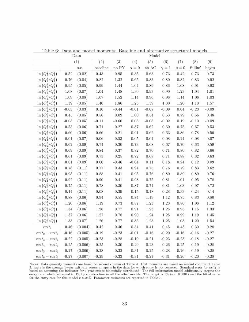
Table 6: Data and model moments: Baseline and alternative structural modelsData Model

(1) (2) (3) (4) (5) (6) (7) (8) (9)

s.e. baseline no PY α = 0 no AC γ = 1 ρ = 0 fullinf bayes

ln(Q2

1/Q11

)0.52 (0.02) 0.43 0.95 0.35 0.63 0.73 0.42 0.73 0.73

ln(Q3

1/Q11

)0.76 (0.04) 0.82 1.32 0.65 0.83 0.80 0.82 0.83 0.92

ln(Q4

1/Q11

)0.95 (0.05) 0.99 1.44 1.04 0.89 0.86 1.08 0.91 0.93

ln(Q5

1/Q11

)1.08 (0.07) 1.04 1.48 1.30 0.93 0.90 1.23 1.04 1.01

ln(Q6

1/Q11

)1.09 (0.08) 1.07 1.52 1.14 0.96 0.96 1.14 1.06 1.03

ln(Q7

1/Q11

)1.39 (0.05) 1.40 1.86 1.25 1.39 1.30 1.20 1.10 1.57

ln(Q2

2/Q21

)-0.03 (0.03) 0.10 -0.44 -0.01 -0.07 -0.09 0.04 -0.23 -0.09

ln(Q3

2/Q31

)0.45 (0.05) 0.56 0.09 1.00 0.54 0.53 0.79 0.56 0.48

ln(Q3

3/Q31

)-0.05 (0.05) -0.11 -0.60 0.05 -0.05 -0.02 0.19 -0.10 -0.09

ln(Q4

2/Q41

)0.55 (0.06) 0.71 0.27 0.87 0.62 0.60 0.75 0.67 0.53

ln(Q4

3/Q41

)0.60 (0.06) 0.66 0.21 0.91 0.62 0.63 0.86 0.78 0.50

ln(Q4

4/Q41

)-0.01 (0.07) -0.06 -0.53 0.05 0.04 0.08 0.24 0.08 -0.07

ln(Q5

2/Q51

)0.62 (0.09) 0.74 0.30 0.73 0.68 0.67 0.70 0.63 0.59

ln(Q5

3/Q51

)0.69 (0.09) 0.84 0.37 0.82 0.70 0.71 0.80 0.82 0.66

ln(Q5

4/Q51

)0.61 (0.09) 0.73 0.25 0.72 0.68 0.71 0.88 0.82 0.63

ln(Q5

5/Q51

)0.01 (0.09) 0.00 -0.46 -0.04 0.11 0.18 0.24 0.12 0.09

ln(Q6

2/Q62

)0.78 (0.11) 0.77 0.33 0.94 0.75 0.76 0.79 0.83 0.62

ln(Q6

3/Q61

)0.95 (0.11) 0.88 0.41 0.95 0.76 0.80 0.89 0.89 0.76

ln(Q6

4/Q61

)0.92 (0.11) 0.90 0.41 0.98 0.75 0.81 1.01 0.95 0.78

ln(Q6

5/Q61

)0.75 (0.11) 0.78 0.30 0.87 0.74 0.81 1.03 0.97 0.72

ln(Q6

6/Q61

)0.14 (0.11) 0.08 -0.39 0.15 0.18 0.28 0.33 0.24 0.14

ln(Q7

2/Q71

)0.88 (0.06) 0.94 0.55 0.84 1.19 1.12 0.75 0.83 0.80

ln(Q7

3/Q71

)1.20 (0.06) 1.19 0.73 0.87 1.23 1.23 0.86 1.08 1.12

ln(Q7

4/Q71

)1.34 (0.06) 1.26 0.77 0.91 1.23 1.25 0.95 1.15 1.33

ln(Q7

5/Q71

)1.37 (0.06) 1.27 0.78 0.90 1.24 1.25 0.99 1.19 1.45

ln(Q7

6/Q71

)1.33 (0.07) 1.26 0.77 0.85 1.23 1.25 1.03 1.20 1.54

exit1 0.46 (0.004) 0.42 0.46 0.54 0.41 0.45 0.43 0.30 0.28

exit2 − exit1 -0.16 (0.005) -0.19 -0.23 -0.01 -0.16 -0.20 -0.16 -0.16 -0.27

exit3 − exit1 -0.22 (0.005) -0.23 -0.28 -0.19 -0.21 -0.23 -0.23 -0.18 -0.27

exit4 − exit1 -0.25 (0.006) -0.25 -0.30 -0.29 -0.23 -0.26 -0.25 -0.19 -0.28

exit5 − exit1 -0.27 (0.006) -0.28 -0.32 -0.31 -0.25 -0.28 -0.26 -0.19 -0.28

exit6 − exit1 -0.27 (0.007) -0.29 -0.33 -0.31 -0.27 -0.31 -0.26 -0.20 -0.28

Notes: Data quantity moments are based on second column of Table 4. Exit moments are based on second column of Table5. exit1 is the average 1-year exit rate across all spells in the data for which entry is not censored. Standard error for exit1 isbased on assuming the indicator for 1-year exit is binomially distributed. The full information model additionally targets theentry rate, which set equal to 1% by construction in all the other models. The target is 1% (s.e. 0.0001) and the fitted valuefor the entry rate for this model is 0.25%. Parameter estimates are reported in Table 7.

33

Table 7: Parameters and fit: Baseline and alternative structural modelsParameter

Model α δ φ γ ρ σν σηF

E(R1)ω λ θ Fit

(1) baseline 0.50 0.46 3.03 0.58 0.40 0.52 0.34 0.31 0.03 n.a. n.a. 3.71

s.e. (0.23) (0.15) (0.00) (0.00) (0.00) (0.00) (0.00) † (0.00)

(2) α = 0 n.a n.a. n.a. 0.49 0.00 0.45 2.56 0.52 0.11 n.a. n.a. 32.44

(3) no AC 0.76 0.80 n.a. 0.87 0.44 0.37 0.19 0.10 0.03 n.a. n.a. 5.46

(4) γ = 1 0.70 0.86 17.63 n.a. 0.31 0.34 0.17 0.12 0.04 n.a. n.a. 6.62

(5) ρ = 0 0.29 0.10 10.23 0.42 n.a. 0.68 1.89 0.40 0.08 n.a. n.a. 19.86

(6) setq n.a. n.a. n.a. 0.96 0.93 0.98 2.00 4.74 0.01 n.a. 36 24.33‡

(7) fullinf 0.29 0.47 13.27 n.a. 0.07 1.95 2.05 0.00 0.05 0.01 n.a. 18.45‡

(8) bayes 0.51 0.29 35.82 n.a. 0.83 0.66 0.16 1.72 0.00 n.a n.a. 16.99

Notes: Standard errors on the baseline parameter estimates are calculated following Gourieroux, Monfort and Renault (1993)as described in the online appendix. † The baseline estimate of F is 0.0131 and the standard error is 0.0105. “Fit” is the valueof the criterion function, m′V m, where m is the difference between data moments and moments of the model conditional onthe parameter vector, and V is a diagonal matrix with the vector of inverses of the standard errors of the data moments onthe diagonal. ‡ For the full information model, the criterion function minimized in the estimation includes the entry rate, butfor comparability the fit value reported here includes only the baseline moments. For the quantity setting model, the criterionfunction minimized in the estimation includes price moments, but for comparability the fit value reported here includes onlythe baseline moments.

Bagwell (2007).42 Our estimated value of φ is nonzero, consistent with adjustment costs a

la Arkolakis (2010). In order to provide some intuition for the magnitude of φ, we calculate

the weighted average expenditure on marketing and advertising (i.e., Aikt + c(Dikt , A

ikt

)) as

a share of revenue. Since φ and θ move together, this share is a function of our baseline

choice of θ. Unfortunately we do not have data on marketing and advertising expenditures

which would allow us to use this to discipline θ. For export spells lasting at least seven years,

33% of revenues are devoted to marketing and advertising in the initial year in a market,

while this declines to just under 23% of revenues by year 6 (see Table A.68 in the online

appendix).43

We find that there is a nontrivial variance of both permanent and mean-reverting id-

iosyncratic demand shocks. Idiosyncratic demand shocks are persistent, but not strikingly

so. Meanwhile, our estimate of γ, the parameter that governs the speed of learning, is equal

to 0.57 on a 6-month basis. This implies that it is only at the beginning of their fourth year

that over 99% of incumbents are informed (see Table A.69 in the online appendix).

We find that there are nontrivial fixed costs of export participation. For the ultimately

successful spells (i.e those lasting at least 7 years), these amount to to 15% of revenue in the

initial year in a market and decline to 6% of revenue by year 6.

42Eaton et al. (2014) report very high rates of attrition of exporter-importer matches, which is consistentwith our finding of a high depreciation rate for customer base.

43Gourio and Rudanko (2014) provide evidence from Compustat for manufacturing and nonmanufacturingfirms, suggesting shares in the range 17-27%.

34

Finally, we estimate a modest probability of the firm-market experiencing a “death

shock,” since ω = 0.03 is the probability of exogenous exit on a 6-month basis. Most of

exit out to seven years in a market is endogenous.

7.3 Restricted versions of the baseline model

We now examine the role played by each of the features of the model by eliminating them one-

by-one, and where appropriate, re-estimating. This is helpful in understanding the mapping

between moments and parameters.

First we assess the contribution of part-year effects to the fit of the baseline model. To

do this, we keep all parameters fixed, but calculate the targeted moments assuming that all

entrants enter at the beginning of a year, rather than half entering in the first 6-month period,

and half entering in the second 6-month period. The implied moments are reported in column

(3) of Table 6. Figures A.54 and A55 in the online appendix illustrate the results. Part-year

effects are key to matching the relationship between initial quantities in 1-year export spells

and initial quantities in longer export spells, but not to matching the relationships between

initial quantities in spells longer than 1 year. They also play a role in matching within-spell

growth rates, not just in the first and last years in a spell, but also to some extent in the

second year of a spell, though they are not responsible for all of within-spell quantity growth.

Finally, they play a role in matching the decline in the exit hazard between year 1 and year

2 in a market, but they are not key to the subsequent behavior of exit.

We next shut down customer capital by setting α = 0. When we do this, the parameters

δ and φ become redundant. Now the only intertemporal choice faced by the firm is whether

or not to participate.44 Column (4) of Table 6 reports the fitted moments and row (2) of

Table 7 reports the estimated parameters of this model, while figures A.56 and A.57 in the

online appendix illustrate the results. This model can generate an increasing relationship

between initial quantities and spell length, but it is incapable of generating within-spell

quantity growth beyond that due to part-year effects and exogenous idioysncratic demand.

In order to try to match within-spell quantity dynamics, the estimated standard deviation

of the mean-reverting component of idiosyncratic demand is very large, which implies that

the fit of the exit trajectory is very poor.

We shut down all adjustment costs of investment by setting φ = 0 and allowing for full

reversibility of investment expenditures (the firm can “consume” inherited D). This means

44This model resembles that of Das et al. (2007), but with the addition of learning about idiosyncraticdemand.

35

that learning and part-year effects are the only sources of dynamics in the model. Column

(5) of Table 6 reports the fitted moments and row (3) of Table 7 reports the estimated

parameters of this model, while Figures A.58 and A.59 in the online appendix illustrate

the results. Somewhat surprisingly, learning is faster in this model than in the baseline.

This model can match the increasing relationship between initial quantities and spell length,

and the reduction in exit hazard with market tenure. Relative to the baseline model, it

has difficulty matching within-spell quantity growth: almost all of the dynamics of within-

spell quantities happen within the first year. This is not a foregone conclusion - with slower

learning, this model could generate dynamics over a longer period, but it appears that slower

learning distorts other moments more than it improves the fit of within-spell quantity growth.

We partially shut down learning by setting γ = 1, which implies that at the end of the first

period, all participants learn their permanent and (lagged) transitory idiosyncratic demand.

The only source of dynamics in quantities after period 2 is due to adjustment costs and

residual dynamics from part-year effects. Column (6) of Table 6 reports the fitted moments

and row (4) of Table 7 reports the estimated parameters of this model, while Figures A.60 and

A.61 in the online appendix illustrate the results. Unsurprisingly, the value of φ increases, as

costs of adjustment substitute for learning in generating post-entry dynamics. The fit of this

model is in fact remarkably similar to the learning-only model, though the fit for quantity

growth is marginally better, while fit of initial quantities and the exit is somewhat worse.

We also estimate the model imposing ρ = 0 (i.e., zero autocorrelation of the transitory

component of the exogenous idiosyncratic demand shock). Column (7) of Table 6 reports

the fitted moments and row (5) of Table 7 reports the estimated parameters, while Figures

A.62 and A.63 in the online appendix illustrate the results. This model is unable to generate

different quantity dynamics in export spells of different lengths (apart from part-year effects

in the year of exit). Although our point estimate of ρ in the baseline model may seem low,

this exercise shows that it is crucial to allow for autocorrelation of transitory idiosyncratic

demand in order to match the different behavior of quantities in short and long export spells.

7.4 Non-nested alternative models

We also examine what happens when we modify the model in ways that are not nested in

our baseline.

We estimate a model where there is no customer base, firms set quantities rather than

prices, and this alone combined with learning about idiosyncratic demand generates dy-

36

namics in quantities.45 With this model, we target price moments in addition to quantity

moments, and we also estimate θ, the price elasticity of demand, since in this model it is

identified by the combination of quantity and price moments. Row (6) of Table 7 reports

the estimated parameters of this model, while Table A.67 and Figures A.64, A.65 and A.66

in the online appendix report the fit of the various moments. In order to match the fact that

there are substantial dynamics of quantities, but no dynamics of prices, the model requires

θ = 36. Notwithstanding this very high value, the estimated model implies that initial prices

are more than 10% higher in spells that last at least 3 years than in spells that last only

1 year, in direct contradiction to the data. It also implies that falling prices signal exit, in

contrast to the data. Finally, the model provides a very poor fit to the exit trajectory, as

learning is estimated to be very fast.

Additionally, we estimate a model without any learning, where firms observe both com-

ponents of their idiosyncratic demand (ν and ηt) before taking any decisions. Column (8) of

Table 6 reports the fitted moments and row (7) of Table 7 reports the estimated parameters,

while Figures A.67 and A.68 in the online appendix illustrate the results. The full informa-

tion model has difficulty matching 1-year exit rates, and the exit trajectory more generally.

It requires very high standard deviations of both components of idiosyncratic shocks in order

to generate a positive relationship between initial quantities and survival.

Finally, we modify our baseline model by assuming that firms are Bayesian, and use the

Kalman filter to update their beliefs about the two components of idiosyncratic demand based

on realizations of quantities. This model is considerably more computationally demanding

to solve and estimate than the other models we consider.46 Column (9) of Table 6 reports

the fitted moments and row (8) of Table 7 reports the estimated parameters, while Figures

A.69 and A.70 in the online appendix illustrate the results. This model overpredicts initial

quantities and growth in the longest spells, and it fails strikingly to match the behavior of

exit, generating too little exit in the first year, and being unable to generate dynamics in exit

beyond the second year. This is because the parameters of the idiosyncratic demand process

necessary to match the behavior of quantities imply very rapid learning: after participating

one period in the market, firms assign 99% probability to their true ν. This shows that the

assumption of slow learning is key to the success of our baseline model.

45This model is similar to that in Berman et al. (2015) and Arkolakis et al. (2017), except that we allowidiosyncratic demand to be autocorrelated (ρ > 0) and model learning as stochastic rather than Bayesian.

46We restrict the SMM algorithm for our estimates of the Bayesian model to 25,000 rather than 50,000independent draws of “firm-markets.” This model still takes an order of magnitude longer to estimate thanthe baseline model.

37

7.5 Summary

To sum up, our baseline model provides a good fit to all the moments of the data. Accu-

mulation of customer base plays a key role in explaining the post-entry dynamics of export

quantities and export prices. Slow learning about idiosyncratic demand is key to match-

ing the behavior of exit. While qualitatively, either costs of adjusting customer base or

slow learning could explain the evolution of quantities and exit, quantitatively both of these

mechanisms are necessary.

8 Implications for adjustment to shocks

We now show that our findings can provide at least a partial answer to a key question

in international macroeconomics and trade: why are short-run elasticities of exports with

respect to prices smaller than long-run elasticities?47 In this section, we simulate our model,

showing that it generates sluggish adjustment in response to shocks. In addition, we show

that it can generate responses to news shocks. This is true even though entry is exogenous

in our model, and there is no general equilibrium feedback through marginal cost. For

illustrative purposes, we focus on shocks to ad valorem tariffs, but the implications are not

limited to this type of shock.

All of our simulations take the same form. We fix all parameters at our baseline estimates.

We solve for the policy functions of the firm under two different tariff environments. We

simulate the behavior of 1,000,000 “firms” for 100 years (i.e. 200 periods) using the initial

policy function in the relevant experiment. This gives us an initial distribution of market

participants in terms of customer base, information and idiosyncratic demand in year 0. In

the first half of year 1, the particular experiment is initiated, and we simulate responses for

20 years (i.e. 40 periods). We also use the same draws for idiosyncratic shocks to simulate

a counterfactual world where tariffs do not change. We then sum exports across all firms in

order to illustrate the implied dynamics of aggregates in both experiment and counterfactual.

8.1 Short vs long run responses to shocks

We first examine the timing of responses to shocks. Demand for each firm is given by:

Qikt =

(τ kt P

ikt

)−θ (Dikt

)αexp

(εikt).

47See e.g. Hooper et al. (2000) and Gallaway et al. (2003).

38

We assume first that tariffs are equal to 5% (τH = 1.05) through year 0. At the begining

of year 1, it is announced, unexpectedly, that in that period and from then on, tariffs will

fall to 0 (τL = 1). We simulate responses of aggregate exports under this experiment, as

well as under the counterfactual where tariffs remain (and are expected to remain) equal to

5% throughout. It is convenient to report the results in terms of the elasticity of aggregate

exports with respect to the shock at different time horizons. We calculate this elasticity as

follows. Let Xt denote aggregate exports at year t in our experiment, and let X ′t denote

aggregate exports at year t in the counterfactual. Similarly, let τt denote the tariff at year

t in our experiment, and let τ ′t denote the tariff at year t in the counterfactual. Then we

calculate the elasticity using:

σt =lnXt − lnX ′tln τt − ln τ ′t

The time series of this elasticity is reported in Figure 9. On impact, the elasticity is 2.7

(note that this is greater than the price elasticity of demand which is given by θ = 2), and

rises to 3.4 after 10 years.

Figure 9: Simulation results: Short vs long run elasticities with respect to tariff shocks

0 2 4 6 8 10 12 14 16 18 20

Year

2.6

2.7

2.8

2.9

3

3.1

3.2

3.3

3.4

3.5

Ela

sticity o

f aggre

gate

export

s w

rt tariff c

hange

← Announcement and tariff change

Tariff decrease

Tariff increase

Notes: Figure shows simulated elasticity of aggregate exports with respect to an unexpected 5% change in tariffs at the beginningof year 1, based on 1 million “firms” and baseline parameter estimates. Costs, foreign demand and entry are held fixed. Source:Authors’ calculations.

In a second version of this exercise, we assume that tariffs are equal to 0 through year 0,

and that the unexpected announcement at the beginning of year 1 is that tariffs have risen

to 5%. The elasticity based on this second exercise and the corresponding counterfactual

39

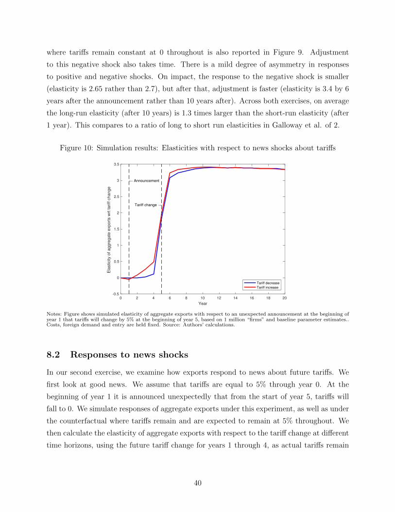
where tariffs remain constant at 0 throughout is also reported in Figure 9. Adjustment

to this negative shock also takes time. There is a mild degree of asymmetry in responses

to positive and negative shocks. On impact, the response to the negative shock is smaller

(elasticity is 2.65 rather than 2.7), but after that, adjustment is faster (elasticity is 3.4 by 6

years after the announcement rather than 10 years after). Across both exercises, on average

the long-run elasticity (after 10 years) is 1.3 times larger than the short-run elasticity (after

1 year). This compares to a ratio of long to short run elasticities in Galloway et al. of 2.

Figure 10: Simulation results: Elasticities with respect to news shocks about tariffs

0 2 4 6 8 10 12 14 16 18 20

Year

-0.5

0

0.5

1

1.5

2

2.5

3

3.5

Ela

sticity o

f aggre

gate

export

s w

rt tariff c

hange

← Announcement

Tariff change →

Tariff decrease

Tariff increase

Notes: Figure shows simulated elasticity of aggregate exports with respect to an unexpected announcement at the beginning ofyear 1 that tariffs will change by 5% at the beginning of year 5, based on 1 million “firms” and baseline parameter estimates..Costs, foreign demand and entry are held fixed. Source: Authors’ calculations.

8.2 Responses to news shocks

In our second exercise, we examine how exports respond to news about future tariffs. We

first look at good news. We assume that tariffs are equal to 5% through year 0. At the

beginning of year 1 it is announced unexpectedly that from the start of year 5, tariffs will

fall to 0. We simulate responses of aggregate exports under this experiment, as well as under

the counterfactual where tariffs remain and are expected to remain at 5% throughout. We

then calculate the elasticity of aggregate exports with respect to the tariff change at different

time horizons, using the future tariff change for years 1 through 4, as actual tariffs remain

40

unchanged during this period:

σt =lnXt − lnX ′t

ln (1.05)− ln (1.00)

The time series of this elasticity is reported in Figure 10. Aggregate exports do respond in

advance of the change in the actual tariff, though the magnitude of the response to positive

news is small.

In a second version of this exercise, we assume that tariffs are equal to 0 through year

0. At the beginning of year 1 it is announced unexpectedly that from the start of year

5, tariffs will rise to 5%. The elasticity based on this experiment (and the corresponding

counterfactual) is also reported in Figure 10. In the case of bad news, there is a non-trivial

response in advance of the change in the actual tariff.

9 Conclusion

We use customs microdata to distinguish between three competing models of demand and

customer base used in the literature on firm dynamics, business cycles, and international

trade. These competing models have quite different predictions about the behavior of prices,

and this is what we exploit to distinguish between them. Our findings on the behavior of

prices are inconsistent with models where firms learn about idiosyncratic demand through

prices, and grow by sliding down their demand curves. More importantly, they are incon-

sistent with models where demand depends on lagged sales, and firms grow by charging

markups below their steady state level, gradually increasing them as sales expand. Models

with this feature have been widely applied in firm dynamics, business cycles, and inter-

national trade. But our findings shift attention away from markups and towards non-price

actions such as marketing and advertising as the key mechanism through which firms acquire

customers and expand sales within a market. They suggest that further research on the role

of marketing and advertising in firm growth, business cycles, and international trade would

be very valuable.

References

[1] Altonji, J. and R. Shakotko (1987), “Do Wages Rise with Job Seniority?” Review of

Economic Studies 54, 437-459.

41

[2] Arkolakis, C. (2010), “Market Penetration Costs and the New Consumers Margin in

International Trade,” Journal of Politicial Economy 118 (6), 1151-1199.

[3] Arkolakis, C. (2016), “A Unified Theory of Firm Selection and Growth,” Quarterly

Journal of Economics 131 (1), 89-155.

[4] Arkolakis, C., T. Papageorgiou, and O. Timoshenko (2017), “Firm Learning and

Growth,” Review of Economic Dynamics, forthcoming.

[5] Bagwell, K. (2007), “The Economic Analysis of Advertising,” in M. Armstrong and

R. Porter, eds., Handbook of Industrial Organization, vol. 3, 1701-1844, Amsterdam:

North-Holland.

[6] Bastos, P., D. A. Dias and O. Timoshenko (2017), “Learning, Prices, and Firm Dynam-

ics,” mimeo.

[7] Berman, N., P. Martin and T. Mayer (2012), “How Do Different Exporters React to

Exchange Rate Changes,” Quarterly Journal of Economics 127, 437-492.

[8] Berman, N., V. Rebeyrol, and V. Vicard (2015), “Demand Learning and Firm Dynam-

ics: Evidence from Exporters,” mimeo.

[9] Das, S., M. J. Roberts and J. R. Tybout (2007), “Market Entry Costs, Producer Het-

erogeneity, and Export Dynamics,” Econometrica 75 (3), 837-873.

[10] Drozd, L. A., and J. B. Nosal (2012a), “Understanding International Prices: Customers

as Capital,” American Economic Review 102 (1), 364-395.

[11] Drozd, L. A., and J. B. Nosal (2012b), “Pricing-to-Market in Business Cycle Models,”

mimeo.

[12] Eaton, J., S. Kortum, and F. Kramarz (2011), “An Anatomy of International Trade:

Evidence From French Firms,” Econometrica 79 (5), 1453-1498.

[13] Eaton, J., M. Eslava, M. Kugler, and J. R. Tybout (2008), “Export Dynamics in Colom-

bia: Firm-Level Evidence,” in E. Helpman, D. Marin, and T. Verdier, eds., The Orga-

nization of Firms in a Global Economy, 231-272, Cambridge, MA: Harvard University

Press.

[14] Eaton, J., M. Eslava, D. Jinkins, C. Krizan, and J. R. Tybout (2014), “A Search and

Learning Model of Export Dynamics,” mimeo.

42

[15] Fitzgerald, D., Y. Yedid-Levi and S. Haller (2017), “Can Sticky Quantities Explain

Exchange Rate Disconnect?” mimeo.

[16] Foster, L., J. Haltiwanger, and C. Syverson (2008), “Reallocation, Firm Turnover, and

Efficiency: Selection on Productivity or Profitability?” American Economic Review 98

(1), 394-425.

[17] Foster, L., J. Haltiwanger, and C. Syverson (2016), “The Slow Growth of New Plants:

Learning About Demand,” Economica 83, 91-129.

[18] Gallaway, M., C. McDaniel and S. Rivera (2003), “Short-run and long-run industry-level

estimates of U.S. Armington elasticities,” North American Journal of Economics and

Finance 14, 49-68.

[19] Gilchrist, S., R. Schoenle, J. Sim and E. Zakrajsek (2017), “Inflation Dynamics During

the Financial Crisis,” American Economic Review 107 (3), 785-823.

[20] Gourieroux, C., A. Monfort and E. Renault (1993), “Indirect Inference,” Journal of

Applied Econometrics 8 (SI), 85-118.

[21] Gourio, F., and L. Rudanko (2014), “Customer Capital,” Review of Economic Studies

81 (3), 1102-1136.

[22] Hall, R. (2014), “What the Cyclical Response of Advertising Reveals About Markups

and Other Macroeconomic Wedges,” NBER Working Paper 18370.

[23] Harrigan, J., X. Ma and V. Shlychkov (2015), “Export Prices of U.S. Firms,” Journal

of International Economics 97, 100-111.

[24] Hooper, P., K. Johnson, and J. Marquez (2000), “Trade Elasticities for the G-7 Coun-

tries,” Princeton Studies in International Economics, 87.

[25] Hottman, C., S. Redding, and D. Weinstein (2016), “Quantifying the Sources of Firm

Heterogeneity,” Quarterly Journal of Economics, forthcoming.

[26] ISGEP (2008), “Understanding Cross-Country Differences in Exporter Premia: Com-

parable Evidence for 14 Countries,” Review of World Economics 144, 596-635.

[27] Jovanovic, B. (1982), “Selection and the Evolution of Industry,” Econometrica 50 (3),

649-670.

43

[28] Lawless, M. (2009), “Firm Export Dynamics and the Geography of Trade,” Journal of

International Economics 77 (2), 245-254.

[29] Pierce, J., and P. Schott (2012), “A Concordance Between Ten-Digit US Harmonized

System Codes and SIC/NAICS Product Classes and Industries,” Journal of Economic

and Social Measurement 37 (1-2), 61-96.

[30] Piveteau, P. (2016), “An Empirical Dynamic Model of Trade with Customer Accumu-

lation,” mimeo.

[31] Rauch, J. (1999), “Networks versus Markets in International Trade,” Journal of Inter-

national Economics 48 (1), 7-35.

[32] Ravn, M., S. Schmitt-Grohe, and M. Uribe (2006), “Deep Habits,” Review of Economic

Studies 73 (1), 195-218.

[33] Ruhl, K., and J. Willis (2016), “New Exporter Dynamics,” International Economic

Review, forthcoming.

[34] Van Beveren, I., A. B. Bernard and H. Vandenbussche (2012), “Concording EU Trade

and Production Data over Time,” mimeo.

44

How Exporters Grow - · PDF fileHow Exporters Grow Doireann Fitzgeraldy Stefanie Hallerz Yaniv...

Documents

Transcript of How Exporters Grow - · PDF fileHow Exporters Grow Doireann Fitzgeraldy Stefanie Hallerz Yaniv...