How exactly does word2vec work?

David Meyer

dmm@{1-4-5.net,uoregon.edu,brocade.com,...}

July 31, 2016

1 Introduction

The word2vec model [4] and its applications have recently attracted a great deal of attentionfrom the machine learning community. These dense vector representations of words learnedby word2vec have remarkably been shown to carry semantic meanings and are useful ina wide range of use cases ranging from natural language processing to network flow dataanalysis.

Perhaps the most amazing property of these word embeddings is that somehow these vectorencodings effectively capture the semantic meanings of the words. The question one mightask is how or why? The answer is that because the vectors adhere surprisingly well to ourintuition. For instance, words that we know to be synonyms tend to have similar vectorsin terms of cosine similarity and antonyms tend to have dissimilar vectors. Even moresurprisingly, word vectors tend to obey the laws of analogy. For example, consider theanalogy ”Woman is to queen as man is to king”. It turns out that

vqueen − vwoman + vman ≈ vking

where vqueen, vwoman, vman and vking are the word vectors for queen, woman, man, andking respectively. These observations strongly suggest that word vectors encode valuablesemantic information about the words that they represent.

Note that there are two main word2vec models: Continuous Bag of Words (CBOW) andSkip-Gram. In the CBOW model, we predict a word given a context (a context can besomething like a sentence). Skip-Gram is the opposite: predict the context given an inputword. Each of these models is examined below.

This document contains my notes on the word2vec. NB: there are probably lots of mistakesin this...

1

Figure 1: Simple CBOW Model

2 Continuous Bag-of-Words Model

The simplest version of the continuous bag-of-word model (CBOW) is a ”single contextword” version [3]. This is shown in Figure 1. Here we assume that there is only one wordconsidered per context, which means the model will predict one target word given onecontext word (which is similar to a bi-gram language model).

In the scenario depicted in Figure 1, V is the vocabulary size and the hyper-parameter Nis the hidden layer size. The input vector x = {x1, x2, . . . , xV } is one-hot encoded, that is,that some xk = 1 and all other xk′ = 0 for k 6= k′.

The weights between between the input layer and the hidden layer can be represented bythe V ×N matrix W. Each row of W is the N -dimensional vector representation vw of theassociated word w in the input layer. Give a context (here a single word), and assumingagain xk = 1 and xk′ = 0 for k 6= k′ (one-hot encoding), then

h = xTW = W(k,.) := vwI (1)

This essentially copies the k-th row of W to h (this is due to the one-hot encoding of x).Here vwI is the vector representation of the input word wI . Note that this implies thatthe link (aka activation) function of the hidden units is linear (g(x) = x). Recall that

WV×N =

w11 w12 . . . w1N

w21 w22 . . . w2N

......

. . ....

wV1 wV2 . . . wVN

(2)

and

2

x =

x1x2...xV

(3)

so that

h = xTW =[x1 x2 . . . xk . . . xV

]

w11 w12 . . . w1N

w21 w22 . . . w2N

......

. . ....

wk1 wk2 . . . wkN

......

. . ....

wV1 wV2 . . . wVN

(4)

=[xkwk1 xkwk2 . . . xkwkN

]# for xk = 1, xk′ = 0 for k 6= k′ (5)

=[wk1 wk2 . . . wkN

]# k-th row of W (6)

= W(k,.) (7)

:= vWI (8)

From the hidden layer to the output layer there is a different weight matrix W′ = {w′i,j}which is a N×V matrix. Using this we can compute a score for each word in the vocabulary:

uj = v′wjT · h (9)

where v′wj is the j-th column of the matrix W′. Note that the score uj is a measure of the

match between the context and the next word 1 and is computed by taking the dot productbetween the predicted representation (v′wj ) and the representation of the candidate targetword (h = vwI).

Now you can use a softmax (log linear) classification model to obtain the posterior distri-bution of words (turns out to be multinomial distribution):

p(wj |wI) = yj =exp(uj)

V∑j′=1

exp(uj′)

(10)

1Though almost all statistical language models predict the next word, it is also possible to model thedistribution of the word preceding the context or surrounded by the context.

3

where yj is the output of the j-th unit of the output layer. Substituting Equations 1 and9 into Equation 10 we get

p(wj |wI) =exp(v′wo

TvwI)

V∑j′=1

exp(v′w′j

TvwI) (11)

Notes

• Both the input vector x and the output y are one-hot encoded

• vw and v′w are two representations of the input word w

• vw comes from the rows of W

• v′w comes from the columns of W′

• vw is usually called the input vector

• v′w is usually called the output vector

2.1 Updating Weights: hidden layer to output layer

The training objective (for one training sample) is to maximize Equation 11, the conditionalprobability of observing the actual output word wO (denote its index in the output layeras j∗) given the input context word wI (and with regard to the weights). That is,

max p(wO|wI) = max yj∗ (12)

= max log yj∗ (13)

= uj∗ − log

V∑j′=1

exp(uj′) := −E (14)

where E = − log p(wO|wI) is our loss function (which we want to minimize), and j∗ isthe index of the actual output word (in the output layer). Note (again) that this lossfunction can be understood as a special case of the cross-entropy measurement betweentwo probabilistic distributions.

The next step is to derive the update equation of the weights between hidden and outputlayers. Take the derivative of E with respect to j-th unit’s net input uj , we obtain

4

∂E

∂uj= yj − tj := ej (15)

where tj = 1(j = j∗), the indicator function, i.e., tj will be 1 when the j-th unit is theactual output word, otherwise tj = 0 . Interestingly this derivative is simply the predictionerror ej of the output layer.

The next step is to take the derivative on w′ij to obtain the gradient on the hidden→ outputweights which (by the chain rule) is

∂E

∂w′ij=∂E

∂uj· ∂uj∂w′ij

= ej · hi (16)

since (sketch of the proof)

∂E

∂uj=

∂

(uj∗ − log

V∑j′=1

exp(uj′)

)∂uj∗

(17)

=∂uj∗

∂uj−∂

(log

V∑j′=1

exp(uj′)

)∂uj

(18)

= tj −exp(uj)

V∑j′=1

exp(uj′)

(19)

= tj − yj # by Equations 10 and 15 (20)

Now, using stochastic gradient descent, we obtain the weight updating equation for hidden→output weights:

w′ij(new)

= w′ij(old) − η · ej · hi (21)

and/or

v′wj(new)

= v′wj(old) − η · ej · h (22)

where η > 0 is the learning rate (standard SGD), ej = yj − tj (Equation 15), hi is the i-thunit in the hidden layer, and v′wj is the output vector for word wj .

5

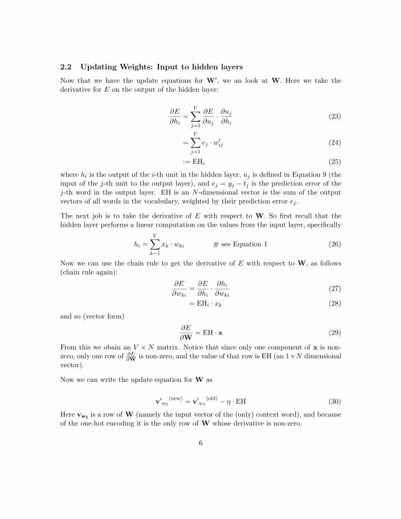
2.2 Updating Weights: Input to hidden layers

Now that we have the update equations for W′, we an look at W. Here we take thederivative for E on the output of the hidden layer:

∂E

∂hi=

V∑j=1

∂E

∂uj· ∂uj∂hi

(23)

=V∑j=1

ej · w′ij (24)

:= EHi (25)

where hi is the output of the i-th unit in the hidden layer, uj is defined in Equation 9 (theinput of the j-th unit to the output layer), and ej = yj − tj is the prediction error of thej-th word in the output layer. EH is an N -dimensional vector is the sum of the outputvectors of all words in the vocabulary, weighted by their prediction error ej .

The next job is to take the derivative of E with respect to W. So first recall that thehidden layer performs a linear computation on the values from the input layer, specifically

hi =V∑k=1

xk · wki # see Equation 1 (26)

Now we can use the chain rule to get the derivative of E with respect to W, as follows(chain rule again):

∂E

∂wki=∂E

∂hi· ∂hi∂wki

(27)

= EHi · xk (28)

and so (vector form)

∂E

∂W= EH · x (29)

From this we obain an V ×N matrix. Notice that since only one component of x is non-zero, only one row of ∂E

∂W is non-zero, and the value of that row is EH (an 1×N dimensionalvector).

Now we can write the update equation for W as

v′wI(new)

= v′wI(old) − η · EH (30)

Here vwI is a row of W (namely the input vector of the (only) context word), and becauseof the one-hot encoding it is the only row of W whose derivative is non-zero.

6

Figure 2: General CBOW Model

3 General Continuous Bag-of-Words Model

4 Skip-Gram Model

The Skip-Gram model was introduced in Mikolov [3] and is depicted in Figure 3. As youcan see, Skip-Gram is the opposite of CBOW; in Skip-Gram we predict the context C givenand input word, where is in CBOW we predict the word from C. Basically the trainingobjective of the Skip-Gram model is to learn word vector representations that are good atpredicting nearby words in the associated context(s).

For the Skip-Gram model we continue to use wwi to denote the input vector of the onlyword on the input layer, and as a result have the same definition of the hidden-layer outputsh as in Equation 1 (again this means h copies a row from the input→ hidden weight matrixW associated with input word wI). Recall that the definition of h was

h = W(k,.) := vwI (31)

Now, at the output layer, instead of outputting one multinomial distribution, we outputC multinomial distributions. Each output is computed using the same hidden → outputmatrix as follows:

7

Figure 3: Skip-Gram Model

p(wc,j = wO,c|wI) = yc,j =exp(uc,j)V∑j′=1

exp(uj′)

(32)

where wc,j is the j-th word on the c-th panel of the output layer. wO,c is the actual c-thword in the output context. Note that wI is the (only) input word. yc,j is the output ofthe j-th unit on the c-th panel of the output layer. Finally, uc,j is the input of the j-th uniton the c-th panel of the output layer.

Said in words, this is the probability that our prediction of the j-th word on the c-th panel,wcj , equals the actual c-th output word, wOc, conditioned on the input word wI.

Now, because the output layer panels share the same weights, we have

uc,j = uc = v′wjT · h, for c = 1, 2, . . . , C (33)

where v′wj is the output vector of the j-th word wj of the vocabulary2.

Given all of this, the parameter update equations are not so different from the one contextword CBOW model. The loss function is changed to

2v′wjis again a column of the hidden→ output weight matrix W′

8

E = − log p(wO,1, wO,2, . . . , w0,C|wI) (34)

= − log

C∏c=1

exp(uc,j∗c )V∑j′=1

exp(uj′)

(35)

= −C∑c=1

uc,j∗c + C · log

V∑j′=1

exp(uj′) (36)

where j∗c is the index of the actual c-th output context word in V 3.

Now, if we take the derivative of E with respect to the net input of every unit on panel ofthe output layer (i.e., uc,j), we get

∂E

∂uc,j= yc,j − tc,j := ec,j (37)

which again is the prediction error on the unit (same as in Equation 15). Now, let EI ={EI1,EI2, . . . ,EIV } (EI is a V -dimensional vector) as the sum of the prediction errors overall context words, that is,

EIj =C∑c=1

ec,j (38)

Now you can find the derivative of E with respect to W′ as follows:

∂E

∂w′ij=

C∑c=1

∂E

∂ucj· ∂ucj∂w′ij

= EIj · hi (39)

Given all of this machinery we can now get the update equation for the hidden→ outputmatrix W′, which might look familiar by this time:

w′ij(new)

= w′ij(old) − η · EIj · hi (40)

or

v′wj(new)

= v′wj(old) − η · EIj · h j = 1, 2, . . . , V (41)

3Recall that logAB = logA+ logB

9

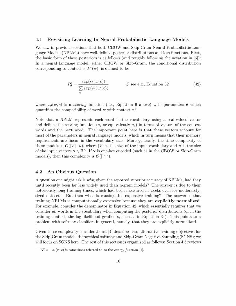
4.1 Revisiting Learning In Neural Probabilisitic Language Models

We saw in previous sections that both CBOW and Skip-Gram Neural Probabilisitic Lan-guage Models (NPLMs) have well-defined posterior distributions and loss functions. First,the basic form of these posteriors is as follows (and roughly following the notation in [6]):In a neural language model, either CBOW or Skip-Gram, the conditional distributioncorresponding to context c, P c(w), is defined to be

P cθ =exp(sθ(w, c))∑

w′exp(sθ(w′, c))

# see e.g., Equation 32 (42)

where sθ(w, c) is a scoring function (i.e., Equation 9 above) with parameters θ whichquantifies the compatibility of word w with context c.4

Note that a NPLM represents each word in the vocabulary using a real-valued vectorand defines the scoring function (sθ or equivalently uj) in terms of vectors of the contextwords and the next word. The important point here is that these vectors account formost of the parameters in neural language models, which in turn means that their memoryrequirements are linear in the vocabulary size. More generally, the time complexity ofthese models is O(|V | · n), where |V | is the size of the input vocabulary and n is the sizeof the input vectors x ∈ Rn. If x is one-hot encoded (such as in the CBOW or Skip-Grammodels), then this complexity is O(|V |2),

4.2 An Obvious Question

A question one might ask is why, given the reported superior accuracy of NPLMs, had theyuntil recently been far less widely used than n-gram models? The answer is due to theirnotoriously long training times, which had been measured in weeks even for moderately-sized datasets. But then what is causing this expensive training? The answer is thattraining NPLMs is computationally expensive because they are explicitly normalized.For example, consider the denominator in Equation 42, which essentially requires that weconsider all words in the vocabulary when computing the posterior distributions (or in thetraining context, the log-likelihood gradients, such as in Equation 34). This points to aproblem with softmax classifiers in general, namely, that they are explicitly normalized.

Given these complexity considerations, [4] describes two alternative training objectives forthe Skip-Gram model: Hierarchical softmax and Skip-Gram Negative Sampling (SGNS); wewill focus on SGNS here. The rest of this section is orgamized as follows: Section 4.3 reviews

4E = −sθ(w, c) is sometimes referred to as the energy function [1].

10

the basics of Parametric Density Estimation, and Section 4.4 describes Noise-ContrastiveEstimation (NCE), where we consider the situation where the model probability densityfunction is unnormalized (recall that the problem with softmax is that it is computationallyexpensive due to the requirement for explicit normalization). Finally, Section 4.6 looks ata modification of NCE called Negative Sampling.

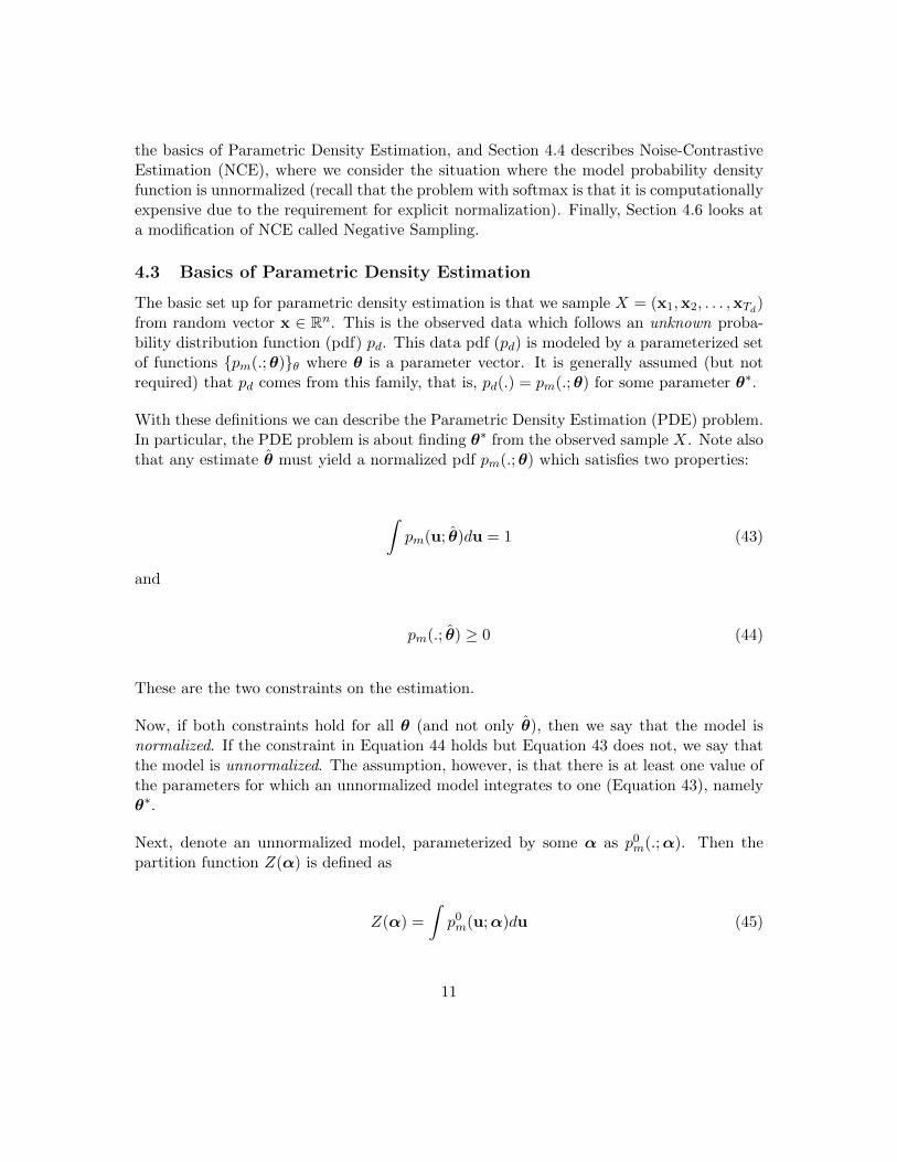
4.3 Basics of Parametric Density Estimation

The basic set up for parametric density estimation is that we sample X = (x1,x2, . . . ,xTd)from random vector x ∈ Rn. This is the observed data which follows an unknown proba-bility distribution function (pdf) pd. This data pdf (pd) is modeled by a parameterized setof functions {pm(.;θ)}θ where θ is a parameter vector. It is generally assumed (but notrequired) that pd comes from this family, that is, pd(.) = pm(.;θ) for some parameter θ∗.

With these definitions we can describe the Parametric Density Estimation (PDE) problem.In particular, the PDE problem is about finding θ∗ from the observed sample X. Note alsothat any estimate θ must yield a normalized pdf pm(.;θ) which satisfies two properties:

∫pm(u; θ)du = 1 (43)

and

pm(.; θ) ≥ 0 (44)

These are the two constraints on the estimation.

Now, if both constraints hold for all θ (and not only θ), then we say that the model isnormalized. If the constraint in Equation 44 holds but Equation 43 does not, we say thatthe model is unnormalized. The assumption, however, is that there is at least one value ofthe parameters for which an unnormalized model integrates to one (Equation 43), namelyθ∗.

Next, denote an unnormalized model, parameterized by some α as p0m(.;α). Then thepartition function Z(α) is defined as

Z(α) =

∫p0m(u;α)du (45)

11

Z(α) can be used to convert the unnormalized model p0m(u;α) into a normalized one:p0m(u;α)/Z(α), which integrates to one for every value of α (as required by Equation 43).

If we rewrite Equation 42 in terms of the partition function Z, can see that

Z(θ) =∑w′

exp(sθ(w′, h)) (46)

P hθ =exp(sθ(w, h))

Z(θ)(47)

Note that I changed the symbol we’re using for the context c to h (also sometimes used forthe context) to avoid name clashes below.

Unfortunately, the function α 7→ Z(α) is defined by the integral in Equation 45 which,unless p0m(.;α) has a particularly convenient form, is likely intractable and/or doesn’t havea nice closed form. In particular, the integral will not be amenable to analytic computationso a closed form for Z(α) can’t be found. In addition, for low-dimensional problems,numerical methods can be used to approximate Z(α) to a very high accuracy (MCMC,Gibbs, or other sampling techniques), but for high-dimensional problems numeric methodsare computationally expensive. Since we are considering the Skip-Gram model here, weare dealing with a PDE problem in high dimension where computation of the partitionfunction is analytically intractable and/or computationally expensive.

4.4 Noise Contrastive Estimation

Noise Contrastive Estimation (NCE) was introduced in [2]. The basic idea is to consider Z(or alternatively c = ln 1/Z) not as a function of α but rather as an additional parameterto the model. Here the unnormalized model p0m(.;α) is extended with an additional nor-malizing parameter (c, note the change in meaning of c from context to the normalizingparameter) and then we estimate

ln pm(.;α) = ln p0m(.;α) + c (48)

with parameters θ = (α, c). The estimate θ = (α, c) is intended to make the unnormalizedmodel p0m(.; α) match the shape of pd and c provides the proper scaling so that the con-straints (Equations 43 and 44) hold. Note that separating estimation of shape and scale isnot possible for maximum likelihood estimation (MLE) since the likelihood can be madearbitrarily large by setting the normalizing parameter c successively larger values.

12

The key observation underlying NCE is that density estimation is largely about charac-terizing properties of the observed data X = (x1,x2, . . . ,xTd), and a convenient way todescribe properties is to describe them relative to the properties of some reference data Y .

Now, assume that the reference (noise) data Y is an iid sample5 (y1,y2, . . . ,yTn) of a ran-dom variable y ∈ Rn with probability distribution function (pdf) pn, and let the (unknown)pdf of X be pd. Then a relative description of the data X can be given by the ratio pd/pnof the two density functions. If the reference distribution pn is known (which it is), we canrecover pd from the ratio pd/pn. That is, since we know the differences between X and Yand also the properties of Y , we can deduce the properties of X. Finally, following [2], weassume that the noise samples are k times more frequent than data samples so data pointscome from the mixture

1

k + 1P hd (w) +

k

k + 1Pn(w) (49)

NCE connects the problem of PDE to supervised learning, in particular to logistic regres-sion, and provides a hint as to how the proposed estimator works: By discriminating, orcomparing, between data and noise, NCE can learn properties of the data in the form ofa statistical model. That is, the key idea behind noise-contrastive estimation is ?learningby comparison?.

So how does this supervised learning work and what exactly does it estimate? Considerfirst the following the notation (which with minor modifications largely follows [2]): LetU = (X∩Y ) = (u1,x2, . . . ,uTd+Tn). NCE then converts the problem of density estimationto a binary classification problem as follows: For each ut ∈ U assign a class label Ct suchthat Ct = 1 if ut ∈ X and Ct = 0 if ut ∈ Y . Now we can use logistic regression to estimatethe posterior probabilities since

P (A) =∑n

P (A ∩Bn) # by the Sum Rule (50)

=∑n

P (A,Bn) # alternate notation (51)

=∑n

P (A|Bn)P (Bn) # by the Product Rule (52)

so that the posterior distribution P (C1|x) for two classes C1 and C2 given input vector xwould look like

5Independent Identically Distributed

13

P (C1|x) =P (x|C1)P (C1)

P (x|C1)P (C1) + P (x|C2)P (C2)(53)

Interestingly, the posterior distribution is related to logistic regression as follows: Firstrecall that the posterior P (C1|x) is

P (C1|x) =P (x|C1)P (C1)

P (x|C1)P (C1) + P (x|C2)P (C2)(54)

Now, if we set

a = lnP (x|C1)P (C1)P (x|C2)P (C2)

(55)

we can see that

P (C1|x) =1

1 + e−a= σ(a) (56)

that is, the sigmoid function. This starts to give us a sense that the sigmoid function isrelated to the log of the ratio of likelihoods of p(x|C1) and p(x|C2), or in our context, pd/pn.

Now, since the pdf pd of x is unknown, we cam model the class-conditional probabilityp(.|C = 1) with pm(.;θ), and the class conditional probability densities are

p(u|C = 1;θ) = pm(u;θ) (57)

p(u|C = 0;θ) = pn(u) (58)

So the prior probabilities are

p(C = 1) =Td

Td + Tn(59)

p(C = 0) =Tn

Td + Tn(60)

14

and the posteriors are therefore

P (C = 1|u;θ) =pm(u;θ)

pm(u;θ) + k · pn(u)(61)

P (C = 0|u;θ) =k · pn(u)

pm(u;θ) + k · pn(u)(62)

where k is the ratio P (C = 0)/P (C = 1) = Tn/Td (remembering that noise samples yi arek times more frequent that data samples xi).

Note that the class labels Ct are Bernoulli-distributed. Recall the details of the Bernoullidistribution: First, the random variable Y takes values yi ∈ {0, 1}. Then the Bernoullidistribution is a Binomial(1, p) distribution, where 0 < p < 1 and P (Y = y) = py(1−p)1−y.The the probability that Yi = yi for i = 1, 2, . . . , n is

P (Y ) =n∏i=1

pyi(1− p)1−yi (63)

and the log likelihood `n(p) is

`n(p) =

n∑i=1

[Yi log p+ (1− Yi) log(1− p)

](64)

Returning to NCE, the log-likelihood of the parameters θ is then

`(θ) =

Td+Tn∑t=1

Ct lnP (Ct = 1|ut;θ) + (1− Ct) lnP (Ct = 0|ut;θ) (65)

=

Td∑t=1

ln[h(xt;θ)

]+

Tn∑t=1

ln[1− h(yt;θ)

](66)

where

G(u; θ) = ln pm(u; θ)− ln pn(u) (67)

h(u; θ) = σ(G(u; θ)) # σ(x) = 1/(1 + e−x) (68)

Optimizing `(θ) with respect to θ leads to an estimate G(.;θ) of the log ratio ln(pd/pn)(see Equation 55 for the derivation). That is, an approximate description of X relative to

15

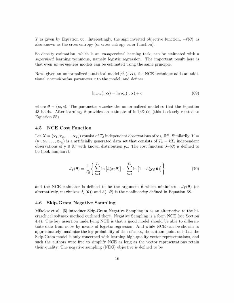
Y is given by Equation 66. Interestingly, the sign inverted objective function, −`(θ), isalso known as the cross entropy (or cross entropy error function).

So density estimation, which is an unsupervised learning task, can be estimated with asupervised learning technique, namely logistic regression. The important result here isthat even unnormalized models can be estimated using the same principle.

Now, given an unnormalized statistical model p0m(.;α), the NCE technique adds an addi-tional normalization parameter c to the model, and defines

ln pm(.;α) = ln p0m(.;α) + c (69)

where θ = (α, c). The parameter c scales the unnormalized model so that the Equation43 holds. After learning, c provides an estimate of ln 1/Z(α) (this is closely related toEquation 55).

4.5 NCE Cost Function

Let X = (x1,x2, . . . ,xTd) consist of Td independent observations of x ∈ Rn. Similarily, Y =(y1,y2, . . . ,xTn) is a artificially generated data set that consists of Tn = kTd independentobservations of y ∈ Rn with known distribution pn. The cost function JT (θ) is defined tobe (look familiar?):

JT (θ) =1

Td

{Td∑t=1

ln[h(x;θ)

]+

Tn∑t=1

ln[1− h(yi;θ)

]}(70)

and the NCE estimator is defined to be the argument θ which minimizes −JT (θ) (oralternatively, maximizes JT (θ)) and h(.;θ) is the nonlinearity defined in Equation 68.

4.6 Skip-Gram Negative Sampling

Mikolov et al. [5] introduce Skip-Gram Negative Sampling in as an alternative to the hi-erarchical softmax method outlined there. Negative Sampling is a form NCE (see Section4.4). The key assertion underlying NCE is that a good model should be able to differen-tiate data from noise by means of logistic regression. And while NCE can be showin toapproximately maximize the log probability of the softmax, the authors point out that theSkip-Gram model is only concerned with learning high-quality vector representations, andsuch the authors were free to simplify NCE as long as the vector representations retaintheir quality. The negative sampling (NEG) objective is defined to be

16

log σ(v′WOTvWI) +

k∑i=1

Ewi∼Pn(w)[

log σ(−v′Wi

TvWI

](71)

which they claim is used to replace every occurrence of logP (wO|wI) in the Skip-Gramobjective (though exactly how this work isn’t discussed).

5 Acknowledgements

17

References

[1] Yoshua Bengio, Rejean Ducharme, Pascal Vincent, and Christian Janvin. A neuralprobabilistic language model. J. Mach. Learn. Res., 3:1137–1155, March 2003.

[2] Michael U. Gutmann and Aapo Hyvarinen. Noise-contrastive estimation of unnormal-ized statistical models, with applications to natural image statistics. J. Mach. Learn.Res., 13:307–361, February 2012.

[3] Tomas Mikolov, Kai Chen, Greg Corrado, and Jeffrey Dean. Efficient estimation ofword representations in vector space. 01 2013.

[4] Tomas Mikolov, Kai Chen, Greg Corrado, and Jeffrey Dean. word2vec, 2014.

[5] Tomas Mikolov, Ilya Sutskever, Kai Chen, Greg S Corrado, and Jeff Dean. Distributedrepresentations of words and phrases and their compositionality. In C.J.C. Burges,L. Bottou, M. Welling, Z. Ghahramani, and K.Q. Weinberger, editors, Advances inNeural Information Processing Systems 26, pages 3111–3119. Curran Associates, Inc.,2013.

[6] Andriy Mnih and Yee Whye Teh. A fast and simple algorithm for training neuralprobabilistic language models. 06 2012.

18