How Does the Financial Crisis Affect Volatility Behavior ...

Int. J. Financ. Stud. 2013, 1, 81–101; doi:10.3390/ijfs1030081

International Journal of

Financial Studies ISSN 2227-7072

www.mdpi.com/journal/ijfs

Article

How Does the Financial Crisis Affect Volatility Behavior and Transmission Among European Stock Markets?

Faten Ben Slimane 1,*, Mohamed Mehanaoui 2,3 and Irfan Akbar Kazi 3,4

1 IRG Institute, University Paris-Est-Marne la Vallée, 5 Boulevard, Descartes-Champs-sur-Marne

77454, France 2 Department of Finance, France Business School, Campus Amiens, 18, place Saint-Michel,

Amiens 80038, France; E-Mail: [email protected] 3 EconomiX, University of Paris West – Nanterre La Défense, 200 avenue de la République,

Nanterre 92001, France; E-Mail: [email protected] 4 IPAG Lab, IPAG Business School, 184, boulevard Saint-Germain, Paris 75006, France

* Author to whom correspondence should be addressed; E-Mail: [email protected];

Tel.: +33-1-60-95-71-08; Fax: +33-1-60-95-70-59.

Received: 24 June 2013; in revised form: 24 July 2013 / Accepted: 2 August 2013 /

Published: 13 August 2013

Abstract: The spread of the global financial crisis of 2008/2009 was rapid, and impacted

the functioning and the performance of financial markets. Due to the importance of this

phenomenon, this study aims to explain the impact of the crisis on stock market behavior

and interdependence through the study of the intraday volatility transmission. This paper

investigates the patterns of linkage dynamics among three European stock markets—France,

Germany, and the UK—during the global financial crisis, by analyzing the intraday

dynamics of linkages among these markets during both calm and turmoil phases.

We apply a VAR-EGARCH (Vector Autoregressive Exponential General Autoregressive

Conditional Heteroscedasticity) framework to high frequency five-minute intraday returns

on selected representative stock indices. We find evidence that interrelationship among

European markets increased substantially during the period of crisis, pointing to an

amplification of spillovers. In addition, during this period, French and UK markets herded

around German market, possibly explained by behavior factors influencing the stock

markets on or near dates of extreme events. Germany was identified as the hub of financial

and economic activity in Europe during the period of study. These findings have important

implications for both policymakers and investors by contributing to better understanding

the transmission of financial shocks in Europe.

OPEN ACCESS

Int. J. Financ. Stud. 2013, 1 82

Keywords: stock market behavior; volatility spillover; financial crisis; high frequency data

1. Introduction

The recent global financial crisis has considerably affected financial markets and is considered the

most devastating crisis since the Great Depression of 1929. According to data from the World

Federation of Exchanges, at the end of 2007 the world equity market capitalization was more than

$64 trillion and sharply declined in 2009 to stand at $49 trillion—a drop of 22%, which is equal to

25% of global GDP for 2009. This crisis, which mainly originated in the US market, spread rapidly

and dangerously to developed and emerging financial markets and to real economy around the world.

A study by Bartram and Bodnar [1] provides a broad analysis of the impact of the crisis on global

equity markets. Focusing on overall market performance, they show that the world market portfolio

total return index continuously declined from mid-September 2008, whereas the 30 day rolling

portfolio of world markets, measuring normal volatility of global markets, increased during the same

period. The regional market return indices experienced a similar pattern of evolution with, however, a

more significant decline in emerging markets, in contrast to developed markets. Comparing the level

of correlation of returns between pre-crisis and crisis period, Bartram and Bolnar [1] point out an

increase of correlation within a regional market. Considering these results, the study highlights the

sudden and relatively unexpected occurrence of this crisis, and raises many questions among

academics and practitioners—notably, concerning the nature of stock market linkages and the response

of markets to shocks.

This paper contributes to these ongoing debates by investigating the interrelationship between

financial markets and their market behavior changes during financial turmoil, especially during periods

of high risk. Studying market interrelationship will provide evidence of their market behavior, whereas

pointing out sudden changes in cross-market linkages after a shock affecting markets will allow better

investigation of the phenomenon of contagion during financial crises. A better understanding of these

issues has become the key to portfolio allocation and risk management activities, and therefore central

for investors, academics and policymakers.

In our analysis, we adopt the definition of Forbes and Rigobon [2], which stipulates that contagion

is “a significant increase in cross-market linkages”. Hence, there is contagion between markets

if the cross-market linkages increased significantly after a shock. However, if these linkages are

continuously at high levels (before and after a shock) there is no contagion, but only interdependence.

As noted by Forbes and Rogobon [2], there are a number of different types of cross-market linkages,

such as the correlation of asset returns, cross-market correlation coefficients, or the transmission of

shocks or volatility.

Since the provocative paper by Forbes and Rogobon [2], there have been an increasing number of

approaches trying to assess contagion during financial crises. The most commonly used approach is

based on the notion of correlation to study cross-market linkages. Focusing on the 1987 crash, King

and Wadhwani [3], and Lee and Kim [4], for instance, find evidence of an increase in stock return

correlations. Calvo and Reinhart [5], and Baig and Goldfajn [6] studied Mexican and Asian crises


respectively, and report correlation shifts during the turmoil periods. With the recent global financial

crisis, there has been renewed interest by academicians and researchers in analyzing of the

transmission of the crisis. By using a factor model to predict returns and correlation as indicative of

contagion, Bekaert et al. [7] find significant evidence of contagion from US markets and the global

financial sector.

Using more advanced techniques, such as a multivariate regime-switching copula model,

Kenourgios et al. [8] investigate contagion on four emerging and two developed markets during five

recent financial crises (the Asian crisis, the Russian crisis, the Technology Bubble Collapse, and the

Brazilian and Subprime Crises). Their empirical results confirm the contagion phenomenon.

Syllignakis and Kouretas [9] investigated the returns correlation among mainly Central and Eastern

European (CEE) emerging markets and the US, Germany, and Russia during financial crises. Using a

dynamic conditional correlations approach, they provide substantial evidence of contagion, mainly due

to herding behavior in the financial markets of the CEE markets. However, during the Asian and

Russian crises and the technology bubble, the hypothesis of financial contagion was refuted.

A second approach of studying cross-market linkages is based on testing for changes in the

cointegrating vector between markets [10], whereas the third approach is to examine international

transmission mechanisms and see to what extent different factors can affect the market during financial

crises [11,12].

A final approach is to use ARCH-GARCH framework to analyze the transmission of volatility

between markets. Dungey and Martin [13], for example, studied spillovers and contagion across

different equity and currency markets during the East Asian crisis, mainly by analyzing the

transmission of volatility across markets. The empirical results prove that the spillover effects were

relatively larger than contagion effects. Considering three emerging market crises (Asian, Russian and

Argentine) and the subprime crisis of 2007, Kenourgios and Padhi [14] used two different empirical

methodologies (Johansen cointegration tests and vector error correction model, and the Asymmetric

Generalized Dynamic Conditional Correlation AG-DCC GARCH model) to investigate financial

contagion. The empirical results provide evidence of the contagion of the subprime, Asian and Russian

crisis. However, mitigated results concerning the Argentine crisis were observed depending on the

methodology used and the markets studied.

Focusing mainly on BRIC’s stock markets (Brazil, Russia, India, China), Aloui et al. [15] show

strong evidence of dependence between markets during the Global Financial Crisis, using copula

functions and GARCH-M model. These results are confirmed by the study of Dimitriou et al. [16].

A related work on contagion attempts to explain the transmission of volatility among stock markets,

generally known as the volatility-spillover literature. Some studies on international spillovers concentrate

on developed markets, especially the US, Japanese and major European markets (e.g., [17–19]). The

conclusions concerning linkage between European and US markets reveal that of European markets

only the UK and German are affected by the US market [18].

Other studies in this strand concentrate on emerging markets. Some focus on analyzing integration

and interdependence in volatility across emerging markets, while others study the link between

developing and developed markets.

Work related to this literature attempts to explain the transmission of shocks, and concentrates on

financial crises and their effects on the evolution of financial spillovers and market behavior. Focusing


on the Asian crisis, Gosh et al. [20] classify three types of stock markets, one influenced by the

US market, the second influenced by the Japanese market, and the third having no link with the other

markets. Contrary to Gosh et al.’s study, Yang et al. [21] report that the US markets affect Asian

markets, whereas Chen et al. [22] report significant integration between US and Asian markets only

during pre- and post-crisis periods.

For the recent financial crisis (2008–2009), Nikkinen et al. [23] report a segmentation of Baltic

stock markets before the crisis and a significant link to European stock markets during the crisis.

Orlowski [24] studied the proliferation of risks in US and European financial markets prior to and

during the crisis. His results show important levels of volatility during financial distress and a

significant increase of risk in only three markets: Germany, Hungary, and Poland. Kenourgios and

Samitas [25] analyze long-term relationships between Balkan emerging markets and various developed

markets during the global financial crisis. Their results show an increase of stock market dependence

during the period of turmoil. Singh et al. [26] examined price and volatility spillovers across North

American, European and Asian stock markets, finding an important regional influence among Asian and

Europeans stock markets.

In this paper, we focus on studying the effect of the Global Financial Crisis on the intraday

volatility transmission of three European markets (France, Germany, and the UK). The methodology

of the study proceeds as follows. First, we identify the date of shock using the structured break test of

Bai and Perron. Second, we apply the Flexible Fourier Form (FFF) procedure in order to use our high

frequency 5 min intraday data and to deal with the problem of seasonality observed in intraday data.

Then, after splitting our data into two periods according to the date of shock—pre-turmoil and

turmoil—we study European markets returns by employing the bivariate vector autoregressive

framework (VAR). According to this model, the returns of a given market are related to past returns of

the same market and to the cross-market current and past returns in another market. Finally, we

investigate the intraday volatility transmission by using an EGARCH model which captures the

asymmetric impact of shocks on volatility.

This paper contributes to the existing literature on three fronts. First, papers such as [24–26]

typically use daily data series to study financial crises, and their impact on market interrelation and

risk. However, according to the literature and in comparison with daily data, high frequency data better

explain the dynamic properties of volatility and their driving forces [27]. Our paper uses high

frequency 5 minute intraday data to study the volatility interactions among equity markets and takes

into account strong intraday seasonality observed in intraday data. Second, we use a more robust

econometric technique to investigate the structural breaks in data, applying Bai and Perron

methodology [28,29] to distinguish between calm and turbulent phases. Considering the two periods

(calm and turbulent), the study makes an original contribution to understanding market behavior

during the global financial crisis and the ongoing debate about financial market theory. The third major

contribution of this paper is to provide empirical evidence, not only on the level of interdependence

between European markets by applying a VAR and EGARCH framework to study cross-market return

and volatility transmission during calm and turmoil periods, but also in investigating the phenomenon

of contagion during the Global Financial Crisis through the study of magnitude of changes in volatility

between the two periods.


The structure of the paper is organized as follows. Section 2 describes the data and specifies the

turmoil period. Section 3 presents the econometric methodology used in the study. Section 4 reports

and discusses the results and a final section concludes.

2. Data and Preliminary Analysis

For empirical analysis, we use two different data sets. First, we use Standard & Poor’s 500

(S&P 500) daily index from 1 January 2004 to 31 December 2010 to identify the start date of the

turmoil period, considered econometrically as the structural break in our data. S&P 500 price index

was obtained from DataStream. Second, we use high frequency 5 min stock market price data of three

stock markets, namely CAC40 (France), DAX30 (Germany), and FTSE100 (UK) from 1 July 2008 to

28 November 2008. Inspired by the event study methodology, and following the methodology used by

many researchers (e.g., [30]), we use a narrow event window, only examining a short period

surrounding the structural break (date of event) in order to provide a deeper insight into the spillover

dynamics. We obtain high frequency data from Tick Data. They consist of 108 trading days and 10,710

observations for each index. Note that, if needed, we apply linear interpolation to replace solitary

5 min price quotes to obtain periodical data. The markets under study open and close at the same time,

i.e., 9.30 CET (Central European Time) and 17.30 CET, so we do not encounter overlapping problems

in our study.

2.1. Turmoil Period Specification

To split our data into two periods (calm and turmoil periods), we need, as a first step, to specify the

crisis phase. Many researchers determine the date of beginning of the crisis based on major economic

and financial events [2,9,13]. This method is in some degree arbitrary [13]. Other researchers use the

Markov regime switching models to distinguish between crisis and pre-crisis periods [13]. In this

paper, we opt for the Bai and Perron test (BP) [28,29] because it clearly identifies the exact dates of

structural break.

BP involves regressing the variable of interest on a constant and then testing for breaks within that

constant. Therefore, it tests the null hypothesis—of no structural break—against a certain number of

breaks. In our case, Bai and Perron may be presented as follows:

P θ ε t = Tk-1 +1,……..Tk, k = 1,...,m +1

where Pt is the stock market price index at time t,θ is the mean of the price in the kth regime,

m represents the length of the time series, and ε represents the error term. BP requires two parameters

for its implementation. First, it requires the minimum number of observations between breaks and

second, it requires maximum number of possible breaks.

According to our results, the date of Structural break is on Friday, 12 September 2008 with 95%

confidence intervals. Note that on 15 September 2008, Lehman Brothers officially announced itself

bankrupt and filed for bankruptcy protection. Markets seem to have already started to respond to the

financial environmental uncertainty one trading day before the official announcement.


2.2. Data Analysis

Table 1 presents a summary of descriptive statistics of the stock index returns of French, German,

and UK markets, categorized for whole period (from 1 July to 28 November 2008), during calm period

(from 1 July to 11 September 2008), and the turmoil period (from 12 September to 28 November 2008).

As expected, all returns are positive during the calm period, whereas these are negative during the

turmoil episode. With regards to standard deviation, which indicates the level of volatility of data, they

significantly increase after the structural break. Note that the skewness coefficients are positive for all

countries except the UK during the calm period. Moreover, the coefficient indicates that distribution is

more asymmetric during the crisis period than the calm period. Also, all indices returns exhibit excess

kurtosis and rise substantially during the second period. This is evidence of the existence of extreme

events. Furthermore, the Jacque-Bera test rejects the normality hypothesis for the three markets for all

subsamples. Finally, all indices returns series are stationary and present ARCH effects (the results are

no reported here).

Figure 1 shows the evolution of French, German and UK stock indices during the period from

1 July 2008 to 28 November 2008. The figure points out high co-movements among the three

European indices during the whole period. From the graph, we can also see that the stock prices were

relatively stable during the period from July 2008 to mid-September. After this date, we observe an

important downward trend.

Figure 1. The evolution of European stock markets indices (1 July 2008 to 28 November 2008).

Figure 2 illustrates the evolution of average intraday volatility of stock markets indices estimated by

absolute returns. Following the literature [31,32], we consider the absolute return |Rt,n | as a measure of

volatility. The figure shows clearly the strong structure of the volatility. The intra-daily volatility

shows the U-shape identified for most of the markets, and suggested by the model of Admati and

Pfleiderer [33], i.e., a strong volatility at the beginning and end of the trading session. This falls back

to a low level until 14.00 CET; afterwards, the activity on the market accelerates significantly with

peaks between 14.00 and 15.00 CET.

2500

3000

3500

4000

4500

5000

5500

6000

6500

7000

01/0

7/20

0803

/07/

2008

07/0

7/20

0810

/07/

2008

07/1

4/20

0807

/16/

2008

07/2

1/20

0807

/23/

2008

07/2

5/20

0807

/30/

2008

01/0

8/20

0805

/08/

2008

08/0

8/20

0812

/08/

2008

08/1

4/20

0808

/19/

2008

08/2

1/20

0808

/27/

2008

08/2

9/20

0802

/09/

2008

05/0

9/20

0809

/09/

2008

11/0

9/20

0809

/16/

2008

09/1

8/20

0809

/22/

2008

09/2

5/20

0809

/29/

2008

01/1

0/20

0806

/10/

2008

08/1

0/20

0810

/10/

2008

10/1

5/20

0810

/17/

2008

10/2

2/20

0810

/24/

2008

10/2

8/20

0810

/31/

2008

04/1

1/20

0806

/11/

2008

11/1

1/20

0811

/13/

2008

11/1

7/20

0811

/20/

2008

11/2

4/20

0811

/26/

2008

CAC40 DAX30 FTSE100


Figure 2. Average intraday volatility evolution in stock markets indices (1 July 2008 to 28

November 2008).

Note: The graph shows the average at intervals of five minutes of Absolute Returns | |of CAC 40

(AbsRCAC), DAX 30 (AbsRDAX) and FTSE100 (AbsRFTSE) indices from July 2008 till the end of

November 2008.

Figure 3 illustrates the average intraday volatility before and during the turmoil period. We can

observe that, even if the U-shape has remained the same, there is, on average, stronger volatility after

the break point. Theses graphs provide evidence of the presence of seasonal structures in our

intra-daily data. In line with Andersen and Bollerslev [27–34] and in order to avoid potential biases,

the series of intraday returns were deseasonalized.

Figure 3. Average intraday volatility before and during the turmoil period.

CAC 40

0.00

0.05

0.10

0.15

0.20

0.25

0.30

0.35

0.40

9:05

9:25

9:45

10:0

510

:25

10:4

511

:05

11:2

511

:45

12:0

512

:25

12:4

513

:05

13:2

513

:45

14:0

514

:25

14:4

515

:05

15:2

515

:45

16:0

516

:25

16:4

517

:05

17:2

5

Average

Absolute Return

Time (CET)

AbsRCAC AbsRDAX AbsRFTSE

0.00

0.10

0.20

0.30

0.40

0.50

0.60

0.70

09:0

5:00

09:3

0:00

09:5

5:00

10:2

0:00

10:4

5:00

11:1

0:00

11:3

5:00

12:0

0:00

12:2

5:00

12:5

0:00

13:1

5:00

13:4

0:00

14:0

5:00

14:3

0:00

14:5

5:00

15:2

0:00

15:4

5:00

16:1

0:00

16:3

5:00

17:0

0:00

17:2

5:00

After break point Before Break point


Figure 3. Cont.

DAX30

FTSE100

3. Methodology Framework

Before studying the spillover dynamics of stock markets indices returns we should, first,

deseasonlize and standardize our high frequency 5 minute intraday data, in order to eliminate outliers

and other anomalies present in such data. Second, we apply a bivariate VAR-EGARCH model to

investigate the volatility and market behavior of the three European markets.

0.00

0.10

0.20

0.30

0.40

0.50

0.60

0.70

09:0

5:00

09:3

0:00

09:5

5:00

10:2

0:00

10:4

5:00

11:1

0:00

11:3

5:00

12:0

0:00

12:2

5:00

12:5

0:00

13:1

5:00

13:4

0:00

14:0

5:00

14:3

0:00

14:5

5:00

15:2

0:00

15:4

5:00

16:1

0:00

16:3

5:00

17:0

0:00

17:2

5:00

After break point Before Break point

0.00

0.10

0.20

0.30

0.40

0.50

0.60

0.70

09:0

5:00

09:3

0:00

09:5

5:00

10:2

0:00

10:4

5:00

11:1

0:00

11:3

5:00

12:0

0:00

12:2

5:00

12:5

0:00

13:1

5:00

13:4

0:00

14:0

5:00

14:3

0:00

14:5

5:00

15:2

0:00

15:4

5:00

16:1

0:00

16:3

5:00

17:0

0:00

17:2

5:00

After Break point Before Break point


Table 1. Descriptive statistics of data.

Whole Period 1 July 2008 to 28 November 2008

Calm Period 1 July 2008 to 12 September 2008

Turmoil Period 13 September 2008 to 28 November 2008

RSCAC RSDAX RSFTS RSCAC RSDAX RSFTS RSCAC RSDAX RSFTS

Mean −0.002332 −0.001905 −0.001426 0.000530 0.001422 0.000463 −0.005036 −0.005047 −0.003211 Median −0.003149 −0.003858 −0.004682 −0.002501 0.000450 −0.002814 −0.004013 −0.009451 −0.008791

Maximum 2.768749 2.838545 2.900669 1.132326 1.395331 1.060863 2.768749 2.838545 2.900669 Minimum −1.673299 −1.791665 −3.044328 −1.090163 −1.079340 −0.842513 −1.673299 −1.791665 −3.044328 Std. Dev. 0.232476 0.243903 0.226617 0.182200 0.185796 0.178694 0.271532 0.288201 0.264012 Skewness 0.103355 0.107824 0.093690 0.071269 0.050567 −0.034998 0.122225 0.133416 0.136466 Kurtosis 6.938096 7.023621 12.08220 4.948796 5.879413 4.397209 6.305681 6.051845 11.88740

Jarque-Bera 6939.780 7245.328 36825.20 827.5778 1799.296 424.2000 2521.581 2153.848 18144.36 Probability 0.000000 0.000000 0.000000 0.000000 0.000000 0.000000 0.000000 0.000000 0.000000

Observations 10,710 10,710 10,710 5,202 5,202 5,202 5,508 5,508 5,508

This table shows the mean, the median, the maximum, the minimum, and the standard deviation (Std. Dev.) of stock indices returns. Note that these data are presented in a

percentage format. The table also shows the skewness, the kurtosis coefficients and the normality test-Jarque-Bera test-of the three European Markets returns indices:

the CAC40 (RSCAC), the DAX30 (RSDAX) and the FTSE (RSFTS). The data are provided for the whole period, the calm and the turmoil period.


3.1. Deseasonalization of Data via the Flexible Fourier Form (FFF)

We clean the high frequency stock price data for outliers and other anomalies before converting

them into continuously compounded returns [35]. The methodology used is the Flexible Fourier Form

(FFF) proposed by Gallant [36]. This methodology was advocated by Andersen and Bollerslev [27,34]

and has the advantage of being practical and robust. The intraday volatility pattern is determined by

modeling intervals of 5 min absolute returns. Following Andersen and Bollerslev [27,34], the following

decomposition of the intraday returns is considered:

(1)

where N refers to the number of high-frequency returns per day, captures the overall volatility level on day t, denotes the periodic intraday volatility component, and , is an independent and

identically distributed (iid) with zero mean and unit variance error term. , is then defined as:

,,

,

(2)

Replacing by an estimate from a daily realized [37] volatility, was obtained. The seasonal pattern

was estimated by using ordinary least square estimation (OLS).

(3)

with

(4)

P indicates the order of the expansion, i.e., the number of sinusoids necessities to reproduce the

profile of the modeled variable. OPEN, CLOSE and OpenUS are dummy variables which characterize

respectively the effect of opening at 9.05 am CET for the European market, 5.30 pm CET close for the

European market and at 3.30 pm CET for the US market opening.

The deseasonalized and standardized intraday returns were then obtained respectively by:

(5)

(6)

3.2. Bi-Variate VAR EGARCH Process

We consider the EGARCH framework introduced by Nelson [38]. This model performs the

GARCH model of Bollerslev [30], mainly due to the fact that it imposes no positivity constraints on

estimated parameters and captures the asymmetric effect on volatility [39]. This so called leverage effect

means that positive and negative error terms have an asymmetric effect on the volatility. Hence,

the volatility increases more after bad news than after good news.

, , ,1/2

t n t n t t nR s N Z

^

, ,( ; , )t n t nX f t n

0 1 3

2

1 2

1 1

( ; , ) sin(2 / ) cos(2 / )( 1) / 2 ( 1)( 2) / 6

P P

p p

p p

n nf t n C N N A pn N B pn N

N N N

Open Close OpenUS

, , ,ˆ/t n t n t nR R f

, , . ,̂ˆ ˆ/t n t n t t nR R f


We use a bivariate VAR-EGARCH model to investigate the volatility of our series of returns of the

CAC40, the DAX30 and FTSE100 indices.

The VAR(k)-EGARCH (1,1) model is given in the following way:

(7)

with i = 1,….n and refers to the stock market index.

Equation (7) is a vector autoregressive (VAR) model of the conditional mean equation of returns

on stock market index i (Ri,t). It means that Ri depends on previous own values of stock returns i (Ri),

the cross-market current and past returns (Rj) and the random variable (εi). The random variable is

conditionally Gaussian,

with the information set containing intradaily price information through period t − 1, and the

diagonal elements of the conditional variance ht may be given as follows:

(8)

where Zt= εt/√ht is the standardized innovation and E(|Zt|) = 2/ .

The second equation of the model (Equation (8)) represents the conditional variance of the stock

market index returns. This equation means that the exponential conditional variance depends on the

lagged value of innovation of the stock returns, the terms to capture asymmetric effects, and lag of

conditional variance of the stock market return index. The parameters αi,j with i = j captures the effect

of the magnitude of a lagged innovation on the conditional variance, and when i ≠ j the coefficient

captures the size and sign effect of a shock to market j on market i. Further, captures the effects of

news from the stock market on the conditional variance (the leverage effect). Hence, allows volatility

to react differently accordingly to the sign of lagged returns (positive versus negative). If γ is negative

and statistically significant, then we have an asymmetric response, i.e., the effect of bad news will be

larger than good news. The last parameter measures the persistence of volatility in the stock market

index returns.

4. Results and Discussion

4.1. FFF Estimates

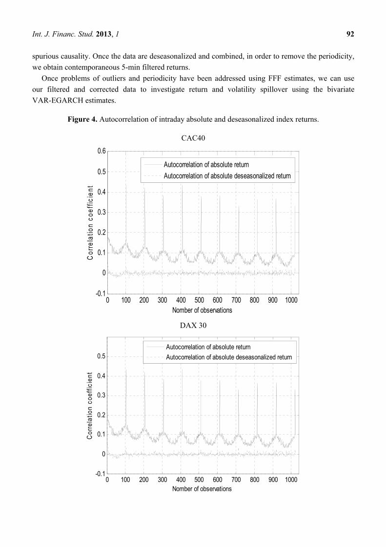
The periodic character of the behaviour of the volatility inside the day of exchange is clearly

illustrated via the correlative structure of autocorrelation of absolute returns [40] in Figure 4. As can be

seen, the autocorrelations of the absolute returns on 10 days present systematic peaks for lags which

correspond to the whole period.

The origin of this stylised feature was the intraday seasonality shown in Figure 2. As we can denote,

the FFF representation considerably reduced the intraday periodicity. As shown in the Figure 4, there

is a significant decay in serial correlation. Therefore, the standardized returns are reducing the risk of

n

j

k

mtimtjjiiti RR

1 1,,,0,,

),0( ~1 ttt hNI

)())(()( 1,,1,,1,1

1,,0,,

tijitjjitj

n

jtjjiiti hLnZZEZhLn


spurious causality. Once the data are deseasonalized and combined, in order to remove the periodicity,

we obtain contemporaneous 5-min filtered returns.

Once problems of outliers and periodicity have been addressed using FFF estimates, we can use

our filtered and corrected data to investigate return and volatility spillover using the bivariate

VAR-EGARCH estimates.

Figure 4. Autocorrelation of intraday absolute and deseasonalized index returns.

CAC40

DAX 30

0 100 200 300 400 500 600 700 800 900 1000-0.1

0

0.1

0.2

0.3

0.4

0.5

0.6

Nomber of observations

Cor

rela

tion

coef

ficie

nt

Autocorrelation of absolute return

Autocorrelation of absolute deseasonalized return

0 100 200 300 400 500 600 700 800 900 1000-0.1

0

0.1

0.2

0.3

0.4

0.5


Cor

rela

tion

coef

ficie

nt




Figure 4. Cont.

FTSE100

Note: The maximum lag length shown on horizontal axis is 10 days. The solid line represents the autocorrelations coefficients for absolute returns and the dotted line the autocorrelations coefficients for absolute deseasonalized returns.

4.2. Modeling Intraday Volatility Specifications and Analysis—Bivariate VAR-EGARCH Estimates

We proceed with the estimation of the bivariate VAR-EGARCH model among the pairs of indices

of: CAC40/DAX30, the CAC40/FTSE100 and the DAX30/FTSE100. Estimation results are reported

in Tables 2–4. The model specification is chosen according to likelihood ratio tests and the minimum

value of the information criteria, while the lag order is selected by Akaike (AIC) and Schwarz (SIC)

information criteria [41].

For all pairs of indices, we note that, in most cases, the parameters of the model are statistically

significant. These results provide evidence of return and volatility spillover among these markets.

Note, however, that the levels of transmission of returns and volatility depend on both the pairs of

markets and the period of study considered. Moreover, the estimated γ coefficients for the asymmetry

effect are significant at the 5% level, which indicate the existence of an asymmetric response of

volatility to shocks and justifies the use of EGARCH model. In the following sections, we analyse the

return and volatility transmission according to each period in order to investigate the interrelationship

among these European markets surrounding the break date.

4.2.1. Market Behaviour during the Calm Period

The VAR terms (βi,j) are estimated from the conditional mean equation of returns Equation (8).

According to Tables 2–4, the estimated β1,2 and β2,1 coefficients indicating respectively the return

transmission from market 2 to market 1 and from market 1 to market 2 are statistically significant.

0 100 200 300 400 500 600 700 800 900 1000-0.1

0

0.1

0.2

0.3

0.4

0.5

0.6


Cor

rela

tion

coef

ficie

nt




This result shows that there is a significant return spillover between the markets, a finding in line with

previous research (e.g., [38]).

Moreover, the results indicate a more significant return spillover from DAX30 to both the CAC 40

and FTSE100, rather than the opposite. For example, considering the pair of indices DAX30/FTSE100,

the parameter β1,2 is not significant, whereas the parameter β21 is significant and equal to 0.1516,

suggesting that roughly 15.16% of the German returns innovation is transferred to the UK stock market.

Table 2. VAR (1) EGARCH (1,1) CAC 40 FTSE 100 estimates.

Variable Before 12 September 2008 After 12 September 2008

Coeff Std Error T-Stat Coeff Std Error T-Stat

β1,0 0.0001 0.0013 0.0594 −0.0068 ** 0.0031 −2.2115 β1,1 −0.0980 *** 0.0203 −4.8173 −0.1269 *** 0.019 −6.6757 β1,2 0.1253 *** 0.023 5.4433 0.1255 *** 0.0184 6.8089 β2,0 0.0003 0.0018 0.1959 −0.0053 * 0.0029 −1.8372 β2,1 0.0409 ** 0.02 2.0482 0.0340 * 0.0187 1.8172 β2,2 −0.0081 0.0223 −0.3648 0.0118 0.017 0.6939 α1,0 −0.6520 *** 0.0788 −8.2732 −0.1839 *** 0.0306 −6.017 α1,1 0.0732 *** 0.0207 3.5432 0.1598 *** 0.0191 8.3607 α1,2 0.1141 *** 0.0213 5.3674 0.0845 *** 0.0149 5.6717 α2,0 −0.5698 *** 0.0062 −91.7875 −0.1912 *** 0.0299 −6.4019 α2,1 0.0558 *** 0.0171 3.2598 0.2253 *** 0.0196 11.4981 α2,2 0.1050 *** 0.0203 5.1841 0.0460 *** 0.0146 3.1477 γ12 0.5602 * 0.3016 1.8571 −0.0938 *** 0.033 −2.8477 γ21 −0.4119 ** 0.1643 −2.5075 −0.2250 *** 0.0828 −2.7162 δ1 0.8087 *** 0.0229 35.2466 0.9287 *** 0.0115 80.783 δ2 0.8344 *** 0.0024 353.2126 0.9278 *** 0.011 84.6729 ρ 0.8060 *** 0.0046 174.3189 0.8329 *** 0.0036 232.3012

QCAC(20) 27.60 p-value 0.119 24.612 p-value 0.326 QFTSE(20) 29.155 p-value 0.098 26.054 p-value 0.128 Q²CAC(20) 25.661 p-value 0.130 21.739 p-value 0.344 Q²FTSE(20) 21.525 p-value 0.202 21.441 p-value 0.550

Note: Data are obtained using 5 min deseasonalized and standardized returns. βi,j are coefficients of the

regression of the VAR equation—conditional mean equation of returns (Equation (7)). The specification and

optimal lags of the VAR equation are chosen according to likelihood ratio tests and Akaike (AIC) and

Schwarz (SIC) information criteria, respectively. The coefficients α, γ and δ are coefficients of the regression

of the conditional variance of returns (Equation (8)). The asymmetric terms γ are statistically significant

witch confirms the use of EGARCH model. The Q-test of correlation Q(20) and Q²(20) does not reject the

null hypothesis of no serial correlation (using 20 lags). CAC40 refers to market 1 and FTSE100 to market 2.

*, **, *** represent statistical significance at 10%, 5% and 1% respectively.


Table 3. VAR (1) EGARCH (1,1) DAX 30 FTSE 100 estimates.


Coeff Std Error T-Stat Coeff Std Error T-Stat β1,0 0.0009 0.0025 0.3609 −0.0051 * 0.0031 −1.667 β1,1 0.0166 0.0209 0.7939 −0.0639 *** 0.0163 −3.9165 β1,2 0.0011 0.0212 0.0508 0.0318 ** 0.0161 1.9744 β2,0 0.0006 0.0024 0.2618 −0.0035 0.003 −1.1677 β2,1 0.1516 *** 0.0197 7.6869 0.0941 *** 0.0164 5.734 β2,2 −0.0915 *** 0.0206 −4.4342 −0.0411 ** 0.0174 −2.3638 α1,0 −0.5183 *** 0.0963 −5.3824 −0.0869 *** 0.0141 −6.1684 α1,1 0.1373 *** 0.0208 6.5894 0.1705 *** 0.0147 11.6273 α1,2 0.0323 0.0205 1.5715 0.0165 0.0117 1.4082 α2,0 −0.4229 *** 0.0792 −5.3407 −0.1270 *** 0.0209 −6.0909 α2,1 0.0758 *** 0.0182 4.152 0.1795 *** 0.0161 11.1249 α2,2 0.0859 *** 0.0209 4.109 0.0681 *** 0.0123 5.53 γ12 −0.049 0.0754 −0.6501 −0.1301 *** 0.0393 −3.3083 γ21 −0.1007 0.0931 −1.0824 −0.0314 * 0.1092 −1.9881 δ1 0.8452 *** 0.0285 29.6699 0.9639 *** 0.0055 174.1163 δ2 0.8770 *** 0.0228 38.4051 0.9508 *** 0.0077 122.8481 Ρ 0.7521 *** 0.0059 127.4695 0.7783 *** 0.0051 151.5845

QDAX(20) 29.602 p-value 0.091 23.048 p-value 0.112 QFTSE(20) 27.648 p-value 0.150 20.226 p-value 0.323 Q²DAX(20) 18.812 p-value 0.564 12.377 p-value 0.749 Q²FTSE(20) 17.303 p-value 0.627 19.255 p-value 0.315








*, **, *** represent statistical significance at 10%, 5% and 1% respectively.

Table 4. VAR (2) EGARCH (1,1) CAC 40 DAX 30 estimates.



β1,0 −0.0003 0.0022 −0.1555 −0.0045 * 0.0025 −1.8015 β1,1 −0.2742 *** 0.0248 −11.0468 −0.1438 *** 0.0189 −7.5974 β1,2 −0.0810 *** 0.0245 −3.3041 0.1649 *** 0.0171 9.655 β1,3 0.3156 *** 0.0231 13.6933 β1,4 0.0475 * 0.025 1.904 β2,0 0.0003 0.0023 0.1407 −0.0050 * 0.0026 −1.8952 β2,1 −0.0375 0.0251 −1.4949 0.0442 ** 0.0184 2.4 β2,2 −0.0217 0.025 −0.868 −0.0767 *** 0.0167 −4.5822 β2,3 0.0441 * 0.0228 1.93 β2,4 −0.002 0.0264 −0.0761 α1,0 −0.5982 *** 0.0898 −6.6635 −0.0251 *** 0.0097 −2.5853 α1,1 0.0373 * 0.0224 1.661 0.0047 *** 0.0007 7.1456 α1,2 0.1748 *** 0.0249 7.014 0.1107 *** 0.0094 11.7436


Table 4. Cont.



α2,0 −0.6357 *** 0.1367 −4.6502 −0.0204 ** 0.009 −2.2539 α2,1 0.0044 0.023 0.1928 0.0046 *** 0.0007 6.954 α2,2 0.1951 *** 0.0272 7.1742 0.1141 *** 0.0082 13.9236 γ12 0.1976 0.2764 0.715 −11.135 *** 0.0785 −141.822 γ21 −0.0893 * 0.0504 −1.7731 0.2671 *** 0.0486 5.5001 δ1 0.8249 *** 0.026 31.7162 0.9894 *** 0.0036 276.041 δ2 0.8099 *** 0.0404 20.0285 0.9908 *** 0.0034 287.5268 ρ 0.8341 *** 0.0038 221.2988 0.8283 *** 0.0044 188.0018

QCAC(20) 27.665 p-value 0.073 25.433 p-value 0.209 QDAX(20) 29.377 p-value 0.059 23.058 p-value 0.310 Q²CAC(20) 32.485 p-value 0.052 21.739 p-value 0.363 Q²DAX(20) 25.211 p-value 0.197 26.162 p-value 0.215








*, **, *** represent statistical significance at 10%, 5% and 1% respectively

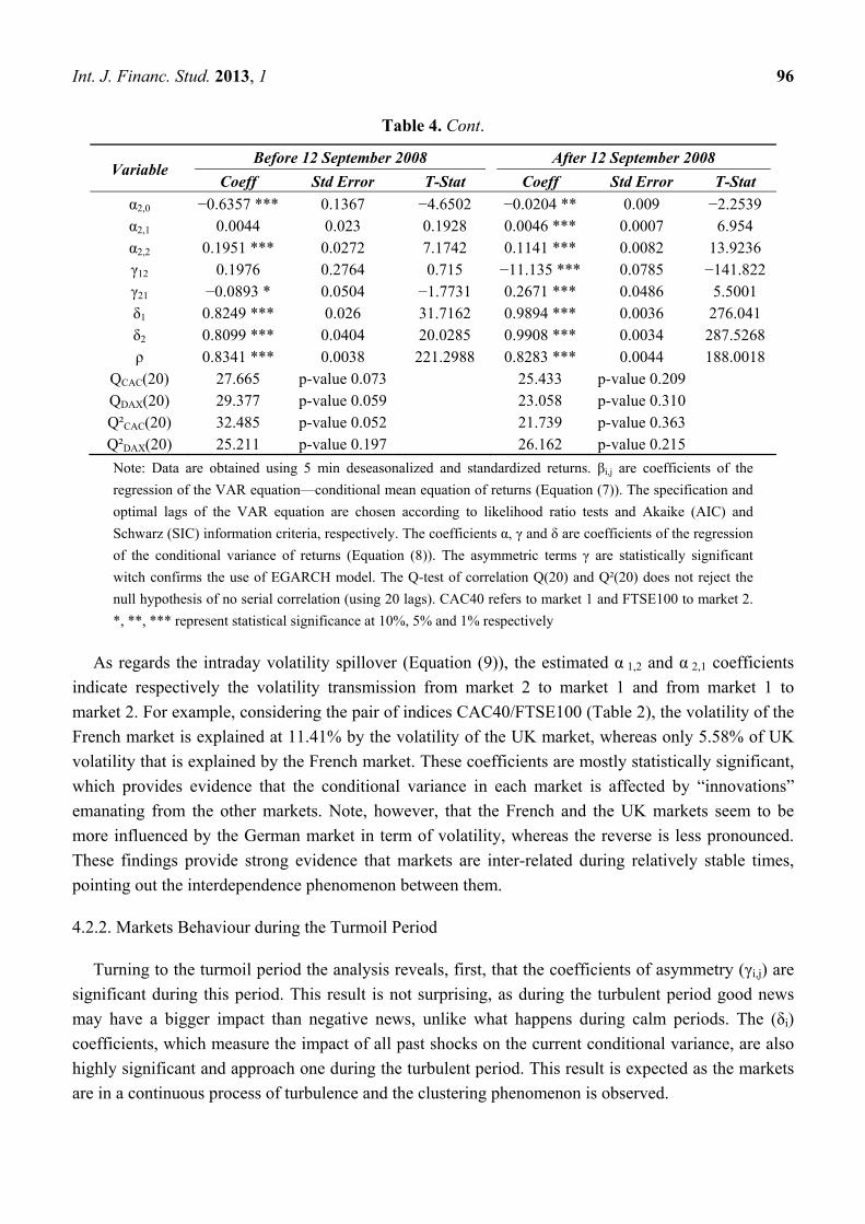
As regards the intraday volatility spillover (Equation (9)), the estimated α 1,2 and α 2,1 coefficients

indicate respectively the volatility transmission from market 2 to market 1 and from market 1 to

market 2. For example, considering the pair of indices CAC40/FTSE100 (Table 2), the volatility of the

French market is explained at 11.41% by the volatility of the UK market, whereas only 5.58% of UK

volatility that is explained by the French market. These coefficients are mostly statistically significant,

which provides evidence that the conditional variance in each market is affected by “innovations”

emanating from the other markets. Note, however, that the French and the UK markets seem to be

more influenced by the German market in term of volatility, whereas the reverse is less pronounced.

These findings provide strong evidence that markets are inter-related during relatively stable times,

pointing out the interdependence phenomenon between them.

4.2.2. Markets Behaviour during the Turmoil Period

Turning to the turmoil period the analysis reveals, first, that the coefficients of asymmetry (γi,j) are

significant during this period. This result is not surprising, as during the turbulent period good news

may have a bigger impact than negative news, unlike what happens during calm periods. The (δi)

coefficients, which measure the impact of all past shocks on the current conditional variance, are also

highly significant and approach one during the turbulent period. This result is expected as the markets

are in a continuous process of turbulence and the clustering phenomenon is observed.


Second, the estimated coefficients indicating the return (β1,2 and β2,1) and the volatility (α 1,2 and

α 2,1) transmission are mostly statistically significant. These results can confirm the strong

interrelationship among markets during turmoil period.

Third, we observe that the German market continues to influence returns and volatility of British

and French markets. Hence, up to 9.41% and to 16.49% of respectively the returns of FTSE100 and

CAC40 indices are explained by German market. Considering the volatility behavior, around 17.95%

of British market volatility is affected by German market. The impact is relatively less important on

French market, where the volatility spillover coefficient α 1,2 is equal to 11.07%.

Focusing on the level of correlation of returns (ρ) between the markets, it increased after the break

date—except for the French-German pair, where the correlation remains relatively constant; the

coefficient between German and UK indices rose from 0.75 to 0.78, and from 0.8 to 0.83 for the

French and UK indices. These results confirm those of Forbes and Rigobon [2], and Ahlgren and

Antell [42] who show that markets are inter-related. Following a crisis or a shock to one country, we

generally observe a significant increase in these cross-market linkages and correlations.

A comparative analysis between calm and turmoil periods shows that, with regards to return

spillover, the magnitude of transmission is roughly the same between the two periods. However, in

term of volatility spillover, the transmission was more important during turmoil periods. Our findings

do not offer evidence of contagion induced by the crisis. The increase of volatility after the structural

break seems to be induced mainly by the interdependence of markets due to normal linkages between

them. These results also confirm previous studies showing that European markets were deeply affected

by US market and shocks emanating from it, which had led to the Global Financial Crisis, e.g., [18].

Moreover, the interrelationship of these European markets was characterized especially by the

influence of the German market on French and UK markets during the whole period of study, and

which increased during turmoil period. This could be explained by the overall composition of the DAX

index as well as the financial and real channels of transmission. Another possible interpretation is

linked to herding behavior on French and UK markets. It seems that German market is seen as the

leader in the Euro Zone, probably due to the fact that it is the world’s fourth largest national economy

(after the USA, Japan, and China) and is furthermore the most important market in the European

Union. Moreover, as was highlighted by many economists and policy makers, the German economy

was the largest contributor to stopping the Eurozone to falling back into recession during the global

financial crisis [43,44]. Hence, it seems that during turmoil periods, a greater attention is given by

European investors to German financial market behavior.

5. Conclusions

This article studies stock market volatility behavior of three European markets, i.e., France,

Germany, and the UK, by analyzing intraday volatility transmission among them during the stocks

market collapse in 2008. To do that, we deseasonalized data using the Flexible Fourier Form and

segmented it into calm and turbulent periods based on the break date (September 12, 2008) estimated

using the Bai-Perron procedure.

The analysis of correlation coefficients shows that the three indices—the DAX 30, CAC 40, and

FTSE 100—are highly intercorrelated, and that these correlations become slightly more important


during the turbulent period. These results support a general pattern of coupling for the three markets

during the whole period of study, with an increase in the coupling during the turmoil phase. This

argument is further supported by the findings of Dimitriou et al. [16]. Moreover, our analysis provides

insights into interdependence structures, intraday return and volatility spillover during the whole

period of study. We also find that, in terms of return spillover between European markets, the

magnitude of transmission is roughly the same between the two periods. Conversely, in term of

volatility spillover, the transmission was more important during turmoil periods. These findings

support the hypothesis that cross-market interactions and dependency are stronger during market

downturns than market upturns [15]. However, the results do not allow us to conclude to the existence

of a pattern of contagion for all markets. The increase of volatility during turmoil period seems to be

mainly due to the interdependence of markets.

Focusing on return and volatility behavior stock markets, we also found that German market

influences French and UK markets, especially during turmoil period. Germany seems to have been

seen as the hub of financial and economic activity in Europe during the period of study. These findings

raise question concerning the role of market consensus versus information during periods of stress. It

would be interesting to incorporate these effects in the empirical modeling to study the behavior of

exchange volatility during the extreme turbulent periods.

Our findings have implications for international investors. Evidence on deep interdependence

between European markets calls into question the advantages of investing in multiple European

markets in order to diversify a portfolio, especially during turmoil periods. On the other hand, since

European markets seem to be widely influenced by German market, special attention should be given

by those who invest in Europe to the economic, financial, and political prospects of Germany.

The results also provide implications for European policy makers about the decisions and directions

to take to better protect markets from contagion and financial collapse. They should examine the

possible strategies to reduce the inter-relationships between markets, and especially to mitigate, as far

as possible, German influence. These findings can also be relevant to Asian policy makers debating the

advantages and disadvantages of increasing financial integration in the region.

In such a financial context—becoming more and more integrated—there is a great interest in

identifying potential gains from international portfolio diversification. This should lead to the

development of more in-depth studies focusing on stock market relationships. Future research could

better explain the role of investor behavior in interdependence of financial markets and impact of

the crisis.

Acknowledgments

The authors would like to thank the anonymous referees for their helpful comments that contributed

to improve the final version of the paper. They would also like to thank the editor for his support

during the review process. Finally, they would like to thank the participants of the 2nd International

Symposium in Computational Economics and Finance (Tunis) and the 19th Annual Conference of the

Multinational Finance Society (Krakow). We are also grateful to Nanci Healy for language editing.


Conflict of Interest

The authors declare no conflict of interest.

References and Notes

1. Bartram, S.; Bodnar, G. No place to hide: The global crisis in equity markets in 2008/2009.

J. Int. Money Financ. 2009, 28, 1246–1292.

2. Forbes, K.; Rigobon, R. No contagion, only interdependence: measuring stock market co-movements.

J. Financ. 2002, 57, 2223–2261.

3. King, M.; Wadhwani, S. Transmission of volatility between stock markets. Rev. Financ. Stud.

1990, 3, 5–33.

4. Lee, S.; Kim, K. Does the October 1987 crash strengthen the co-movements among national stock

markets? Rev. Financ. Econ. 1993, 3, 89–102.

5. Calvo, S.; Reinhart, C. Private Capital Flows to Emerging Markets after the Mexican Crisis;

Calvo, G., Goldstein, M., Hochreiter, E., Eds.; Institute for International Economics: Washington,

DC, USA, 1996; pp. 151–171.

6. Baig, T.; Goldfajn, I. Financial market contagion in the Asian crisis. IMF Staff Pap. 1999, 46,

167–195.

7. Bekaert, G.; Ehrmann, M.; Fratzcher, M.; Mehl, J. Global Crises and Equity Market Contagion;

NBER Working Paper Series #17121; National Bureau of Economic Research, Inc.: Cambridge,

MA, USA, 2011.

8. Kenourgios, D.; Samitas, A.; Paltalidis, N. Financial crises and stock market contagion in a

multivariate time-vaying asymmetric framework. J. Int. Financ. Mark. Inst. Money 2011, 21, 92–106.

9. Syllignakis, M.; Kouretas, G. Dynamic correlation analysis of financial contagion: Evidence from

the central and eastern European markets. Int. Rev. Econ. Financ. 2011, 20, 717–732.

10. Longin, F.; Solnik, B. Is the international correlation of equity returns constant: 1960–1990?

J. Int. Money Financ. 1995, 14, 3–26.

11. Eichengreen, B.; Rose, A.; Wyplosz, C. Contagious currency crises: First test. Scand. J. Econ.

1996, 98, 463–484.

12. Forbes, K. Are Trade Effects Significant in the International Transmission of Crises? In Proceedings

of NBER Conference on Currency Crises Prevention 2000, Cheeca Lodge, Islamorada, FL, USA,

11–13 January 2001; University of Chicago Press: Chicago, IL, USA, 2002.

13. Dungey, M.; Martin, V. Unravelling financial market linkages during crises. J. Appl. Econ. 2007,

22, 89–119.

14. Kenourgios, D.; Padhi, P. Emerging markets and financial crises: Regional, global or isolated

shocks? J. Multinatl. Financ. Manag. 2012, 22, 24–38.

15. Aloui, R.; Ben Aïssa, M.; Nguyen, D. Global financial crisis, extreme interdependences, and

contagion effects: The role of economic structure? J. Bank. Financ. 2011, 35, 130–141.

16. Dimitriou, D.; Kenourgios, D.; Simos, T. Global financial crisis and emerging stock market

contagion: A multivariate FIAPARCH-DCC approach. Int. Rev. Financ. Anal. 2013, 30, 46–56.


17. Baele, L. Volatility spillover effects in European equity markets. J. Financ. Quant. Anal. 2005,

40, 373–401.

18. Savva, C.; Osborn, D.; Gill, L. Spillovers and correlations between US and major European stock

markets: The role of the euro. Appl. Financ. Econ. 2009, 19, 1595–1604.

19. Bartram, S.; Taylor, S.; Wang, Y. The Euro and European financial market. J. Bank. Financ.

2007, 51, 1461–1481.

20. Ghosh, A.; Saidi, R.; Johnson, K. Who moves the Asia-Pacific stock markets–US or Japan?

Empirical evidence based on the theory of cointegration. Financ. Rev. 1999, 34, 159–170.

21. Yang, J.; Kolari, J.; Min, J. Stock market integration and financial crises: The case of Asia.

Appl. Financ. Econ. 2003, 13, 477–486.

22. Chen, C.; Chiang, T.; So, M. Asymmetrical reaction to US stock-return news: Evidence from

major stock markets based on a double-threshold model. J. Econ. Bus. 2003, 55, 487–502.

23. Nikkinen, J.; Piljak, V.; Äijö, J. Baltic stock markets and the financial crisis of 2008–2009.

Res. Int. Bus. Financ. 2012, 26, 398–409

24. Orlowski, L.T. Financial crisis and extreme market risks/Evidence from Europe. Rev. Financ. Econ.

2012, 21, 120–130.

25. Kenourgios, D.; Samitas, A. Equity market integration in emerging Balkan markets. Res. Int. Bus.

Financ. 2011, 25, 296–307.

26. Singh, P.; Kumar, B.; Pandey, A. Price and volatility spillover across North American, European

and Asian stock markets. Int. Rev. Financ. Anal. 2010, 19, 55–64.

27. Andersen, T.G.; Bollerslev, T. Deutsche mark-dollar volatility: Intraday activity patterns,

macroeconomic announcements, and longer run dependencies. J. Financ. 1998, 53, 219–265.

28. Bai, J.; Perron, P. Estimating and testing linear models with multiple structural changes.

Econometrica 1998, 66, 47–78.

29. Bai, J.; Perron, P. Computation and analysis of multiple structural change models. J. Appl. Econ.

2003, 18, 1–22.

30. Bollerslev, T. Generalized autoregressive conditional heteroskedasticity. J. Econ. 1986, 31, 307–327.

31. Taylor, J.; Xu, X. The incremental volatility information in one million foreign exchange

quotations. J. Empir. Financ. 1997, 4, 317–340.

32. Taylor, J. Modelling Financial Time Series; John Willey & Sons: Chichester, UK, 1986.

33. Admati, A.; Pfleiderer, D. A theory of intraday patterns: Volume and price variability.

Rev. Financ. Stud. 1988, 1, 3–40.

34. Andersen, T.G.; Bollerslev, T. Intraday periodicity and volatility persistence in financial markets.

J. Empir. Financ. 1997, 4, 115–158.

35. We calculate returns using the equation Ri,t = 100 × (lnPi,t – lnPi,t-1) where Ri,t is the return for

stock market index i at time t, ln(Pi,t) is the log of stock price at time t, and ln(Pi,t-1) is the log of

the laged value of the stock price at time t. Following Andersen et al. (2000), we delete the return

inverval 9.00–9.05 CET to avoid statistical inference.

36. Gallant, A.R. On the bias in flexible functional forms and an essentially unbiased form: The

fourier flexible form. J. Econ. 1981, 15, 211–245.


37. We assume that: E(Rt,n) = 0, E(Rt,n , Rs,m) = 0 and that the variance and covariance of squared

returns exist and are finite. The continuously compounded daily squared returns may be

decomposed as: Rt ² = (∑Rt,n²).

38. Nelson, D.B. Conditional heteroskedasticity in asset pricing: A new approach. Econometrica

1991, 59, 347–370.

39. Hentschel, L. All in the family: Nesting symmetric and asymmetric GARCH models. J. Financ. Econ.

1995, 39, 71–104.

40. Following Andersen et al. (2000), we delete 9.00-9.05 CET return interval to avoid

statistical inference.

41. We use VAR(1)-EGARCH (1,1) for the three bivariate relations during calm and turbulent periods

except for the CAC40/DAX30 pair during the calm phase where a VAR(2)-EGARCH(1,1) is

more appropriate.

42. Ahlgren, N.; Antell, J. Stock market linkages and financial contagion: A cobreaking analysis.

Q. Rev. Econ. Financ. 2010, 50, 157–166.

43. Organisation for Economic Co-operation and Development (OECD). Economic Survey of

Germany 2010; OECD Publishing: Paris, France, 2010.

44. Anderson, R. German Economic Strength: The Secrets of Success. BBC News, 15 August 2012.

Available online: http://www.bbc.co.uk/news/business-18868704 (accessed on 15 August 2012).

© 2013 by the authors; licensee MDPI, Basel, Switzerland. This article is an open access article

distributed under the terms and conditions of the Creative Commons Attribution license

(http://creativecommons.org/licenses/by/3.0/).

How Does the Financial Crisis Affect Volatility Behavior ...

Documents

Transcript of How Does the Financial Crisis Affect Volatility Behavior ...