How Does Industry Affect Firm Financial Structure? and Phillips 2005.pdf · 2008. 7. 1. · means...
34
How Does Industry Affect Firm Financial Structure? Peter MacKay Hong Kong University of Science and Technology Gordon M. Phillips University of Maryland and NBER We examine the importance of industry to firm-level financial and real decisions. We find that in addition to standard industry fixed effects, financial structure also depends on a firm’s position within its industry. In competitive industries, a firm’s financial leverage depends on its natural hedge (its proximity to the median industry capital–labor ratio), the actions of other firms in the industry, and its status as entrant, incumbent, or exiting firm. Financial leverage is higher and less dispersed in concentrated industries, where strategic debt interactions are also stronger, but a firm’s natural hedge is not significant. Our results show that financial structure, technology, and risk are jointly determined within industries. These findings are consistent with recent industry equilibrium models of financial structure. Despite extensive financial structure research since Myers (1984) and Harris and Raviv (1991) surveyed the literature, important questions remain about how financial structure is related to industry and about how real and financial decisions are related. 1 Although it is widely held that industry factors are important to firm financial structure, empirical evidence shows that there is wide variation in financial structure even after controlling for industries. 2 Researchers routinely remove industry fixed effects by including dummy variables or sweeping out industry This paper was previously circulated under the title: ‘‘Is There an Optimal Industry Financial Structure?’’. MacKay is from the Edwin L. Cox School of Business, Southern Methodist University and Phillips is from the Robert H. Smith School of Business, University of Maryland. We wish to thank Murray Frank, Gerald Garvey, Mike Long, Robert McDonald, Vojislav Maksimovic, Dave Mauer, Nagpurnanand Prabhala, Alexander Reisz, Michael Roberts, Antoinette Schoar, Harry Turtle, Toni Whited, two anon- ymous referees, and seminar participants at the American Finance Association, the Atlanta Finance Consortium, the Northern Finance Association, the Rutgers Conference on Capital Structure, MIT, Southern Methodist University, the University of Delaware, the University of Kentucky, and the Uni- versity of British Columbia for helpful comments. MacKay can be reached at [email protected], homepage http://www.bm.ust.hk/fina/staff/pmackay.html. Phillips can be reached at [email protected], homepage www.rhsmith.umd.edu/Finance/gphillips/. The authors alone are responsible for the work and any errors or omissions. 1 Recent empirical papers on financial structure examine static trade-off and pecking-order theories (Shyam-Sunder and Myers, 1999, Fama and French, 2002, Frank and Goyal, 2003), taxes (Graham, 1996, 2000), managerial fixed effects (Bertrand and Schoar, 2002), technology (MacKay, 2003), and stock returns (Welch, 2004). 2 Bradley, Jarrell, and Kim (1984), Chaplinsky (1983), and Remmers et al. (1974). ª The Author 2005. Published by Oxford University Press. All rights reserved. For Permissions, please email: [email protected] doi:10.1093/rfs/hhi032 Advance Access publication August 31, 2005
Transcript of How Does Industry Affect Firm Financial Structure? and Phillips 2005.pdf · 2008. 7. 1. · means...

How Does Industry Affect Firm Financial
Structure?
Peter MacKay
Hong Kong University of Science and Technology
Gordon M. PhillipsUniversity of Maryland and NBER
We examine the importance of industry to firm-level financial and real decisions. We
find that in addition to standard industry fixed effects, financial structure also
depends on a firm’s position within its industry. In competitive industries, a firm’s
financial leverage depends on its natural hedge (its proximity to the median industry
capital–labor ratio), the actions of other firms in the industry, and its status as
entrant, incumbent, or exiting firm. Financial leverage is higher and less dispersed
in concentrated industries, where strategic debt interactions are also stronger, but a
firm’s natural hedge is not significant. Our results show that financial structure,
technology, and risk are jointly determined within industries. These findings are
consistent with recent industry equilibrium models of financial structure.
Despite extensive financial structure research since Myers (1984) and
Harris and Raviv (1991) surveyed the literature, important questions
remain about how financial structure is related to industry and about
how real and financial decisions are related.1 Although it is widely held
that industry factors are important to firm financial structure, empirical
evidence shows that there is wide variation in financial structure even
after controlling for industries.2 Researchers routinely remove industryfixed effects by including dummy variables or sweeping out industry
This paper was previously circulated under the title: ‘‘Is There an Optimal Industry Financial Structure?’’.MacKay is from the Edwin L. Cox School of Business, SouthernMethodist University and Phillips is fromthe Robert H. Smith School of Business, University of Maryland. We wish to thank Murray Frank,Gerald Garvey, Mike Long, Robert McDonald, Vojislav Maksimovic, Dave Mauer, NagpurnanandPrabhala, Alexander Reisz, Michael Roberts, Antoinette Schoar, Harry Turtle, Toni Whited, two anon-ymous referees, and seminar participants at the American Finance Association, the Atlanta FinanceConsortium, the Northern Finance Association, the Rutgers Conference on Capital Structure, MIT,Southern Methodist University, the University of Delaware, the University of Kentucky, and the Uni-versity of British Columbia for helpful comments. MacKay can be reached at [email protected], homepagehttp://www.bm.ust.hk/fina/staff/pmackay.html. Phillips can be reached at [email protected],homepage www.rhsmith.umd.edu/Finance/gphillips/. The authors alone are responsible for the workand any errors or omissions.
1 Recent empirical papers on financial structure examine static trade-off and pecking-order theories(Shyam-Sunder and Myers, 1999, Fama and French, 2002, Frank and Goyal, 2003), taxes (Graham,1996, 2000), managerial fixed effects (Bertrand and Schoar, 2002), technology (MacKay, 2003), and stockreturns (Welch, 2004).
2 Bradley, Jarrell, and Kim (1984), Chaplinsky (1983), and Remmers et al. (1974).
ª The Author 2005. Published by Oxford University Press. All rights reserved. For Permissions, please email:
doi:10.1093/rfs/hhi032 Advance Access publication August 31, 2005
means and using the remaining variation to test how firm characteristics
affect financial policy. Yet, this approach does not tell us how industry
affects firm financial structure, nor why financial structure and real-side
characteristics vary so widely across firms within a given industry. In
addition, theoretical models such as Dammon and Senbet (1988) and
Leland (1998) stress the jointness of real and financial decisions—yet little
is known about the empirical relevance of the simultaneity of these
decisions. We thus examine these two unresolved but related questions:How important are industry factors to firm financial structure? Can indus-
try equilibrium forces explain how firms distribute within industries—both
along real-side and financial dimensions?
We address these questions by examining how intra-industry variation in
financial structure relates to industry factors and whether real and financial
decisions are jointly determined within industries. We base our analysis on
models of competitive-industry equilibrium (Maksimovic and Zechner,
1991, Williams, 1995, and Fries, Miller, and Perraudin, 1997).3 Similar toMiller’s (1977) irrelevance result, these models illustrate how conclusions
reached in a partial-equilibrium framework are fundamentally altered, even
reversed, as the equilibrium setting is aggregated to the level of an industry.
Our research therefore goes beyond tests of static trade-off and pecking-
order theories to examine whether the decisions of individual firms are
related to those of industry peers. We also investigate the impact of
endogeneity, both as an empirical matter and as an implication of recent
theory, by contrasting single- and simultaneous-equation regressions forfinancial leverage, capital–labor ratios, and cash-flow volatility.
We precede our examination of industry equilibrium models with a
broader investigation of inter- and intra-industry variation in financial
structure. We document extensive cross-sectional variation in financial
leverage in our sample of 315 competitive manufacturing industries.
Regressing firm-level financial leverage on industry-level medians, we
find that most of the variation in financial structure arises within indus-
tries rather than between industries. Specifically, we find that industryfixed effects account for only 13% of variation in financial structure. In
contrast, firm fixed effects explain 54% of variation in financial structure,
and the remaining 33% is within-firm variation.
Given the relative unimportance of industry fixed effects in explaining
financial structure, we examine whether other industry-related factors can
account for some of the wide variation observed within industries. Our
empirical strategy is to construct various measures of a firm’s industry
position inspired from industry equilibrium models and test whether these
3 Chevalier (1995), Phillips (1995), and Kovenock and Phillips (1995, 1997) show that financial structureconditions real decisions in imperfectly competitive industries. Opler and Titman (1994) show that highlyleveraged firms lose market share in concentrated industries after negative industry shocks.
The Review of Financial Studies / v 18 n 4 2005
1434
measures help explain firm financial structure. These include the similar-
ity of a firm’s capital–labor ratio to the industry median, the actions of its
industry peers, and its status as an entrant, incumbent, or exiting firm. We
focus on competitive industries but also examine concentrated industries
to establish the general applicability of our findings.
Consistent with competitive-industry equilibrium models, we find that
financial structure decisions are made simultaneously with technology
and risk choices and that all three decisions are impacted by a firm’sposition within its industry. We find that firms near the industry median
capital–labor ratio use less financial leverage than firms that deviate from
the industry median capital–labor ratio. This is consistent with the idea of
a natural hedge in Maksimovic and Zechner (1991) where firms at the
technological core of an industry experience lower cash-flow risk and use
less debt than firms at the technological fringe. We also find that changes
to a firm’s real and financial characteristics are inversely related to
changes in the same variables made by other firms in its industry. Theseinteractions are consistent with the adjustment patterns predicted by
Maksimovic and Zechner, where the equilibrium process drives firms to
react differently to common industry shocks.
We find contrasting results for concentrated industries. Our natural
hedge proxy is neither statistically nor economically significant in con-
centrated industries, confirming that competitive-industry models per-
form poorly in concentrated industries. However, we find that the
sensitivity of own-firm decisions to industry-peer decisions is muchgreater for firms in concentrated industries, consistent with the impor-
tance of strategic interaction in these industries.
We also investigate the dynamic industry equilibria developed by
Williams (1995) and Fries, Miller, and Perraudin (1997), where entry
and exit are endogeneized. First, we find that, although statistically sig-
nificant, firm reversion to industry medians is economically unimportant.
Second, we find that firm characteristics evolve slowly and that firms tend
to retain their industry rankings. Indeed, we find high persistence inincumbents’ industry position along real and financial dimensions, sug-
gesting that industry equilibrium forces may act to sustain intra-industry
diversity rather than smooth it away. However, our multivariate results
show no important differences between incumbents and entrants. Thus,
while there is some support for the static industry equilibrium modeled in
Maksimovic and Zechner (1991), we find only limited support for the
more intricate models of dynamic industry equilibrium represented by
Williams (1995) and Fries, Miller, and Perraudin (1997).This paper makes two contributions. First, we show that firm financial
structure is determined by industry-related factors other than industry
fixed effects. Consistent with competitive-industry equilibrium models,
we find that proxies for a firm’s position within its industry add both
Importance of Industry to Firm-Level Financial and Real Decisions
1435
statistical and economic significance in explaining its real and financial
decisions. This suggests that, although stylized, these models do provide a
useful framework to explain individual firm behavior.
Second, we identify and account for the interactions between financial
structure, technology, and risk choice. We find that accounting for the
simultaneity of these decisions is important economically—not just econ-
ometrically. Accounting for this simultaneity impacts multiple relations,
including the relations between financial leverage, capital–labor ratios,and cash-flow volatility.
Overall, our paper begins to bridge the gap between empirical studies of
partial-equilibrium models, which simply use firm variation to test repre-
sentative-firm behavior, and industry equilibrium models, which endo-
genize firm variation and link firm-level decisions to broader equilibrium
forces. The remainder of the paper is organized as follows. Section 1
reviews the financial-structure literature and discusses the empirical impli-
cations of the industry equilibrium models. Section 2 describes our datasources, sample selection, and the variables we use to examine these
implications. Section 3 discusses our univariate and multivariate results.
Section 4 concludes.
1. The Importance of Industry to Financial Structure
This section reviews the theoretical models relevant to our analysis.
Although our primary focus is on how financial structure is determined
in perfectly competitive industries, we briefly discuss models of imperfect
competition for comparison and to provide more background on how
industry affects financial structure.
Early theory on the interaction of finance and product markets (Brander
and Lewis, 1986, Maksimovic, 1988) deals with symmetric firms in con-centrated industries and thus cannot explain why competing firms
would choose different financial structures. Other theory examines
how product-market competition is affected when firms have asymmetric
financial structures (Bolton and Scharfstein, 1990, Rotemberg and Scharf-
stein, 1990). Neither this research nor partial-equilibrium theory can
explain why real and financial firm characteristics vary so widely within
industries.
A more recent line of theoretical research by Maksimovic and Zechner(1991), Williams (1995), and Fries, Miller, and Perraudin (1997) stresses
equilibrium forces in the spirit ofMiller (1977). These models show how real
and financial decisions are jointly determined within competitive industries.4
This approach offers additional insights relative to partial-equilibrium
4 The jointness of real and financial decisions is also central to a number of partial-equilibrium models suchas Dammon and Senbet (1988), Mauer and Triantis (1994), and Leland (1998). MacKay (2003) findssignificant empirical interactions between real-side flexibility and financial structure.
The Review of Financial Studies / v 18 n 4 2005
1436
models, namely, that firmsmake their individual real and financial decisions
in reference to the collective decisions of industry peers, and that equili-
brium outcomes imply intra-industry diversity rather than industry-wide
targets.5
Maksimovic and Zechner (1991) assume that firms can choose between
a ‘‘safe’’ technology with a certain marginal cost, and a ‘‘risky’’ technology
with an uncertain cost. In partial equilibrium, no debt is issued since
shareholders would expropriate bondholder wealth by picking the riskytechnology. However, each firm has an incentive to finance with debt and
adopt the risky technology because by allowing firms to raise (lower)
output in good (bad) states, the risky technology initially has greater
expected profits and risk than the safe technology. As more firms pick
the risky technology, the price of output more closely tracks that technol-
ogy’s marginal cost; the risky technology becomes less risky and less
profitable. Equilibrium obtains when the expected value of the ex-ante
safe and risky technologies is equal and firms are indifferent betweenhigh-debt/high-risk and low-debt/low-risk configurations. Thus, what
Maksimovic and Zechner (1991) show is that in industry equilibrium,
firm financial structure is irrelevant because a technology’s risk and
profitability depend not only on ex-ante characteristics but also on how
many firms adopt that technology.
Two implications follow from Maksimovic and Zechner’s analysis.
First, firms near the median industry technology benefit from a risk-
reducing ‘‘natural hedge’’. Such firms will use less financial leveragethan firms whose technology departs from the industry norm. Second,
to preserve equilibrium, firms within an industry make offsetting adjust-
ments to their debt and technology.
Williams (1995) extends Maksimovic and Zechner’s (1991) model by
endogenizing entry and exit and adding exogenous perks consumption.
Williams assumes that firms produce a homogeneous good using either a
high variable-cost, labor-intensive technology with no capital outlay, or a
low variable-cost, capital-intensive technology requiring capital-marketfinancing. Because managers cannot credibly commit to forego their
perks, capital is rationed in equilibrium even though the capital market
is perfectly competitive. Even as the cost of entry converges to zero, a core
of capital-intensive firms earns positive profits because managerial agency
prevents the fringe of labor-intensive firms from raising capital and dis-
sipating the core firms’ monopoly rents.
Like Maksimovic and Zechner (1991), Williams (1995) characterizes
the equilibrium industry distribution of debt and firm characteristics and
5 Almazan andMolina (2002) contrast multiple explanations for the dispersion in financial structure withinindustries. Their analysis complements ours in that they focus on explaining the variation in financialstructure while we test implications of industry equilibrium models for firm-level financial and real-sidedecisions.
Importance of Industry to Firm-Level Financial and Real Decisions
1437
explains firm heterogeneity within industries. By allowing for entry, Williams
predicts an asymmetric equilibrium industry structure characterized by a
core of large, stable, profitable, capital-intensive, financially-leveraged firms
flanked by a competitive fringe of small, risky, non-profitable, labor-intensive
firms.
Fries, Miller, and Perraudin (1997) use a contingent-claims approach to
analyze optimal financial structure in a competitive-industry equilibrium
that combines features of the previous models. Like Williams (1995), theyallow for endogenous firm entry and exit. Like Maksimovic and Zechner
(1991), they incorporate shareholder–bondholder conflicts and corporate
debt tax-shields. Fries, Miller, and Perraudin (1997) find that as a result
of a trade-off between tax advantages and agency costs, a firm optimally
adjusts its financial leverage upward after it enters the industry.
The overarching implication of these models is that own-firm decisions
are partly determined by the position a firm occupies within its industry.
In Maksimovic and Zechner (1991), industry position refers to how closelya firm’s technology compares to the rest of its industry. In Williams (1995)
and Fries, Miller, and Perraudin (1997), industry position refers to whether
a firm belongs to the core or fringe of its industry or its status as entrant,
incumbent, or exiting firm. These models also show that firm decisions
within an industry are interdependent and that firm heterogeneity arises as
an equilibrium outcome. Section 2 describes the specific empirical strategies
we employ to test these implications.
On a broader level, our contribution is in examining the central theme
of these models—that firms’ debt, technology, and risk decisions are
jointly determined within industries—not in testing one model against
the others. Note that we do not conduct structural tests of these models
but rather test the implications that industry position and peer actions
matter, and the central theme that real and financial decisions are simul-
taneously determined as result of industry equilibrium forces.
To examine this central theme, we estimate simultaneous-equation
regression models for financial leverage, capital–labor ratios, and cash-flow volatility. Empirically, as well as theoretically, we allow the financial-
structure decision to depend on technology and risk choice and vice versa.
We account for interactions between these dependent variables by includ-
ing each of the remaining two variables as regressors for the dependent
variables featured in each equation. We use generalized method of
moments (GMM) to reflect the correlation of the residuals across these
equations and to instrument endogenous right-hand-side variables. We
include measures of a firm’s industry position, such as the similarity of itscapital–labor ratio to the industry median capital–labor ratio, the actions
of firms inside and outside its industry-year peer group, and its status as
entrant, incumbent, or exiting firm, to test the idea that firms’ decisions are
affected by those of their industry peers.
The Review of Financial Studies / v 18 n 4 2005
1438
2. Data, variable construction, and methodology
We examine active and inactive firms from the merged COMPUSTAT-
CRSP set produced by Wharton Research Data Services (WRDS). We use
COMPUSTAT for the financial accounting and operating variables. We
use CRSP for historical industry classifications because COMPUSTAT
only reports current industry classifications. We merge in COMPUSTAT’s
business-segment files to compute diversification Herfindahls. Using these
segment files limits the sample to 1981–2000.COMPUSTAT codifies why firms drop out from the sample (note 35,
‘‘reason for deletion’’). We use this variable to distinguish between true
firm exit (Chapter 11 bankruptcy and Chapter 7 liquidation) and firms
whose CUSIP changes because of corporate restructuring. This allows us
to examine the behavior of firms that enter, stay, or leave their industry as
a test of the dynamic industry models developed by Williams (1995),
Fries, Miller, and Perraudin (1997) and Poitevin (1989).
We collect four-digit SIC industry concentration ratios (Herfindahl–Hirschman Index, HHI) from the Census of Manufacturers for 1982,
1987, 1992, and 1997. The Census of Manufacturers reports the results
of the U.S. Census Bureau’s Economic Census held every 5 years. This
provides us with an independent and reasonably timely measure of
industry concentration. An independent measure of industry concentra-
tion is preferable for two reasons. First, rather than rely on the avail-
ability of COMPUSTAT data, the Census of Manufacturers offers the
broadest coverage available and thus helps minimize selection bias andclassification error. Second, the Department of Justice (DOJ) and other
regulatory agencies use the HHI to set and enforce competition policy.
Thus, the HHI is appropriate because it affects both government and firm
behavior and is observable to all.6
2.1 Sample selection
The models we discussed earlier make different assumptions regarding
industry competition. Motivated by the predictions of Maksimovic andZechner (1991), Williams (1995), and Fries, Miller, and Perraudin (1997)
under perfect competition, we form a sample of firms operating in com-
petitive industries by retaining industries with a HHI under 1000.7 To
benchmark our results and investigate models of imperfect competition
(Brander and Lewis, 1986, 1988, Maksimovic, 1988, 1990, etc.), we also
form a sample of firms operating in concentrated industries by retaining
6 We thank the referee for this suggestion. The previous version of the paper relied on the number of firmson COMPUSTAT operating in each industry.
7 This follows the industry classification scheme used by the U.S. Department of Justice and Federal TradeCommission (1997): Unconcentrated industries (HHI under 1000), moderately concentrated industries(HHI from 1000 to 1800), and highly concentrated industries (HHI over 1800).
Importance of Industry to Firm-Level Financial and Real Decisions
1439
industries with a HHI over 1800. For a sharper contrast between competi-
tive and concentrated industries, we exclude industries with a HHI between
1000 and 1800, which the DOJ considers ‘‘moderately concentrated’’.
Because the models we consider build on classical notions of industry and
technology, such as capital–labor ratios, we limit our sample to firms
operating in manufacturing industries, namely, SIC 2000 to 3990. We
exclude firms in industries classified as miscellaneous by dropping indus-
tries where the last two digits of the four-digit SIC code end in ninety-nine.In addition to dropping observations with incomplete data, we delete
observations with negative sales or assets, and those with a CRSP perma-
nent number or capital–labor ratio equal to zero. To prevent influential
observations from skewing our results, we delete outliers as follows. We
drop observations where Tobin’s q is over ten, earnings before interest
and taxes divided by assets is less (more) than negative (positive) two, or
financial leverage lies outside the [0,1] interval.8
The regressions presented in Section 3 control for firm fixed effects byfirst-differencing the firm-level variables (we also control for interacted
industry-year fixed effects). The GMM regressions appearing in that
section use the second lags in levels as instruments. Hence, observations
without at least two lags of data ultimately fall out of the sample.9 The
final sample forms an unbalanced panel of 3074 firms (17,140 firm-years)
operating in 315 competitive industries and 309 firms (1630 firm-years)
operating in 46 concentrated industries.
2.2 Proxies and variable construction
We measure financial leverage as total debt divided by total assets (book
leverage). Using book values may be justified by a recent survey by
Graham and Harvey (2001) who report that managers focus on book
values when setting financial structure. Furthermore, Barclay, Morellec,
and Smith (2003) show how book leverage is theoretically preferable in
regressions of financial leverage, arguing that using market values in the
denominator might spuriously correlate with explanatory variables suchas Tobin’s q. However, Welch (2004) argues against book leverage in
favor of market leverage, and Fama and French (2002) find strikingly
different results for book leverage and market leverage. In light of this
recent controversy, we rerun our regressions using total debt divided by
the market value of equity plus the book value of debt and preferred stock
minus deferred taxes (market leverage).
8 Our base results use the book value of equity to compute financial leverage. As a robustness check, wererun our regressions using the market value of equity and relax the screening interval on financialleverage to [0,2].
9 Because the sample is highly unbalanced, with some firms appearing only a few years and othersremaining throughout the entire panel, this number of lags reflects a trade-off between reducing endo-geneity bias, losing observations and statistical power, and introducing large-firm and survivor biases.
The Review of Financial Studies / v 18 n 4 2005
1440
We use fixed-capital stock (net property, plant, and equipment, in
millions of dollars) divided by the number of employees as a proxy
for capital intensity (the capital–labor ratio, K/L).10 To measure risk,
we use the standard deviation of operating cash flow divided by total
assets using up to ten (minimum four) annual observations.11 Profit-
ability is earnings before interest expense and taxes (EBIT) (data item
13 minus 14) divided by total assets. We measure diversification as
one minus the Herfindahl of output calculated across a firm’s four-digitSIC industries (computed from segment data). This measure equals
zero for single-segment firms and tends toward one for multi-segment
firms. We control for diversification directly and for robustness,
repeat our tests for single-segment firms only. Following Barclay,
Morellec, and Smith (2003) and others, we control for the investment
opportunity set with Tobin’s q (market value of equity plus the book
value of debt and preferred stock minus deferred taxes, divided by
book assets).
2.2.1 Industry position variables. We construct two measures of a firm’s
position within its industry. First, we develop a proxy that captures
Maksimovic and Zechner’s (1991) natural hedge idea. The natural
hedge proxy must possess three properties: (1) it must reflect a firm’s
production technology; (2) it must measure the distance between a firm’s
technology and the typical technology in the firm’s industry, and (3) it
must be comparable across industries. We use the capital–labor ratio tomeasure technology. This variable is specifically modeled in Williams
(1995) and is true to the spirit of the safe-versus-risky cost structure
discussed by Maksimovic and Zechner. We define the typical technology
as the median capital–labor ratio for a given industry and year. This
industry-year median is weighted by each firm’s market share of sales
and excludes the firm itself. We use the absolute value of the difference
between firm’s capital–labor ratio and the industry-year median capital–
labor ratio because natural hedge should only measure how similar ordissimilar a firm is to the rest of its industry, not whether the firm has a
10 COMPUSTAT’s employment number (data item #29) is rarely used in the empirical finance literature, sowe test the quality of this variable on three fronts: coverage, reliability, and stickiness. Coverage: Keepingonly observations where the fixed-capital stock is neither missing nor zero, we find that only about 6% ofobservations are missing the number of employees. This percentage is even lower if we screen on theavailability of other variables used in the study. Reliability: We randomly picked ten firms in 1997 andcross-checked the COMPUSTAT number against what the firms report in their 10-Ks. All concurred100%. Stickiness: We count how many times we observe employment changes of exactly zero. Thishappens about five percent of the time. We exclude these observations from our sample. However,including them makes no material difference to our main conclusions.
11 We also tried using twenty quarterly data points to compute risk. Although this should increase samplesize by requiring fewer consecutive years of firm data, in practice, going to quarterly data results in asmaller sample because the coverage of the quarterly dataset is poor. Results using quarterly data tocompute risk (deseasonalized or not) are substantially the same as those presented here.
Importance of Industry to Firm-Level Financial and Real Decisions
1441
high or low industry-adjusted capital–labor ratio.12 We then divide this
deviation by the range of capital–labor ratio deviations in each industry-
year; this bounds the natural hedge proxy between zero and one and
makes it comparable across industries. For ease of interpretation, we
subtract this value from one. A natural hedge value of one indicates that
the firm’s capital–labor ratio is identical to the industry-year median
capital–labor ratio. A natural hedge value of zero indicates that the
firm’s capital–labor ratio is the furthest from the industry-year mediancapital–labor ratio.
Thus, our natural hedge measure can be expressed algebraically as follows
NHf ,i,y ¼ðK=LÞf ,i,y �mediani,y,�f ðK=LÞ���
���range ðK=LÞf ,i,y �mediani,y,�f ðK=LÞ
������8 f 2 i,y
n o 2 ½0,1�
where f stands for firm, i for industry, and y for year.Because our natural hedge is built solely around the capital–labor
ratio, it might fail to reflect other dimensions of a firm’s position in its
industry. To address this issue, our regressions control for the mean
change in the dependent variables (financial leverage, capital–labor
ratios, and cash-flow volatility) inside and outside a firm’s industry-
year quantile (intra- and extra-quantile). Intra-quantile change is the
mean change in the dependent variable within the industry half to which
a firm belongs. To avoid hardwiring a spurious correlation into theanalysis, the mean change for each firm’s own quantile excludes that
firm itself. Extra-quantile change is the mean change in the other half of
the industry. We construct the quantiles themselves from the lagged
levels of the dependent variables.
2.3 Regression model specification
Our main regressions are simultaneous-equation regressions where finan-
cial leverage, capital–labor ratios, and cash-flow volatility appear both asdependent variables and as regressors in the other two equations. We
include the measures of a firm’s industry position described above,
namely, natural hedge, intra- and extra-quantile change, and dummy
variables for firm entry and exit. These are the main variables of interest
in this study. To ensure that these measures of industry position do not
simply reflect static trade-off and pecking-order theories, we also include
standard control variables such as profitability, firm size (log of total
assets), diversification, and Tobin’s q.
12 Note that natural hedge is distinct from firm-level operating leverage. We focus separately on operatingleverage by including the capital–labor ratio both as an explanatory variable in our regressions and as adependent variable for one of the regression equations.
The Review of Financial Studies / v 18 n 4 2005
1442
Our identification strategy reflects two objectives, namely, to control
for firm fixed effects and to address endogeneity bias. Whited (1992)
shows how both these objectives can be achieved in the context of
GMM estimation with panel data. Specifically, we use year-to-year
changes in the variables (first differences) rather than the levels of the
variables to control for firm fixed effects. Using year-to-year changes
rather than regular firm fixed effects enables us to use twice-lagged levels
of the same variables as instruments. We also adjust the variables forinteracted industry-year fixed effects in order to isolate intra-industry
variation.13 We estimate the following system of simultaneous equations
using GMM:
DLeverage ¼ f ðDcapital=labor, Drisk; Dindustry position,
Dcontrols, fixed effectsÞ þ ~�
DCapital=labor ¼ gðDleverage, Drisk; Dindustry position,
Dcontrols, fixed effectsÞ þ ~"
DRisk ¼ gðDleverage, Dcapital=labor; Dindustry position,
Dcontrols, fixed effectsÞ þ ~!
where D is the first-difference operator, ~�, ~", and ~! are random error
terms, and the endogenous right-hand side variables (financial leverage,
capital–labor ratio, or cash-flow volatility, and natural hedge, profitabil-
ity, size, diversification, and Tobin’s q) are instrumented using their twice-lagged values and other instruments discussed later. For comparability
with prior studies and to show the impact of controlling for endogeneity
and simultaneity, we also estimate the equations separately using ordin-
ary least squares (OLS).
3. Results
We begin by examining how much variation in financial structure arises
between and within industries. After a graphical examination of the
extent of variation in financial structure, our research design is then to
present summary statistics, univariate regressions, transition frequencies,
and multivariate regressions—all examining the importance of industry tofirm decisions.
3.1 Variation in financial structure between and within industries
Figure 1 shows how financial structure varies between and within indus-
tries. We construct these figures as follows. First, we average each firm’s
debt-to-asset ratio over all years it appears in the panel. Next, we calcu-
late the standard deviation of these firm averages across firms within each
13 From this point on we refer to these adjustments as ‘‘industry-year adjusted’’.
Importance of Industry to Firm-Level Financial and Real Decisions
1443
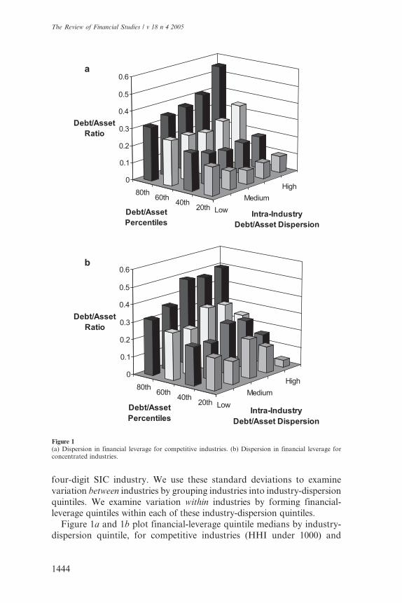
four-digit SIC industry. We use these standard deviations to examine
variation between industries by grouping industries into industry-dispersion
quintiles. We examine variation within industries by forming financial-leverage quintiles within each of these industry-dispersion quintiles.
Figure 1a and 1b plot financial-leverage quintile medians by industry-
dispersion quintile, for competitive industries (HHI under 1000) and
Low
Medium
High
20th40th
60th80th
0
0.1
0.2
0.3
0.4
0.5
0.6
Debt/Asset
Ra
a
b
tio
Debt/Asset
PercentilesIntra-Industry
Debt/Asset Dispersion
Low
Medium
High
20th40th
60th80th
0
0.1
0.2
0.3
0.4
0.5
0.6
Debt/Asset
Ratio
Debt/Asset
PercentilesIntra-Industry
Debt/Asset Dispersion
Figure 1(a) Dispersion in financial leverage for competitive industries. (b) Dispersion in financial leverage forconcentrated industries.
The Review of Financial Studies / v 18 n 4 2005
1444
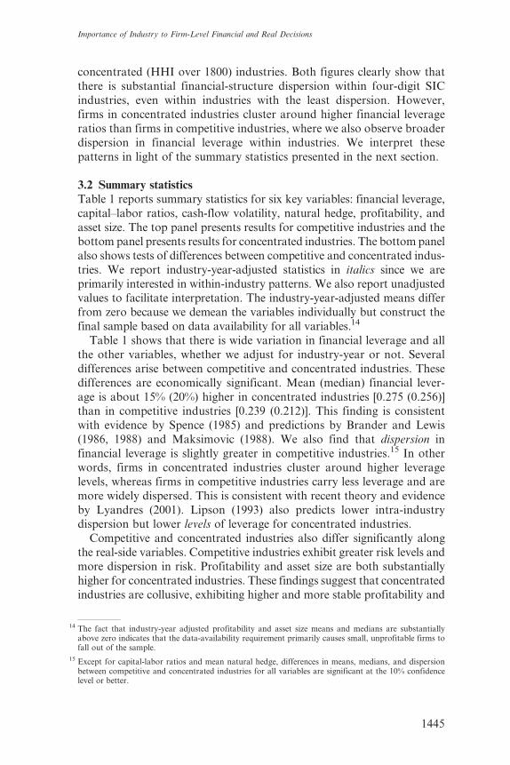
concentrated (HHI over 1800) industries. Both figures clearly show that
there is substantial financial-structure dispersion within four-digit SIC
industries, even within industries with the least dispersion. However,
firms in concentrated industries cluster around higher financial leverage
ratios than firms in competitive industries, where we also observe broader
dispersion in financial leverage within industries. We interpret these
patterns in light of the summary statistics presented in the next section.
3.2 Summary statistics
Table 1 reports summary statistics for six key variables: financial leverage,
capital–labor ratios, cash-flow volatility, natural hedge, profitability, and
asset size. The top panel presents results for competitive industries and the
bottom panel presents results for concentrated industries. The bottom panel
also shows tests of differences between competitive and concentrated indus-
tries. We report industry-year-adjusted statistics in italics since we are
primarily interested in within-industry patterns. We also report unadjustedvalues to facilitate interpretation. The industry-year-adjusted means differ
from zero because we demean the variables individually but construct the
final sample based on data availability for all variables.14
Table 1 shows that there is wide variation in financial leverage and all
the other variables, whether we adjust for industry-year or not. Several
differences arise between competitive and concentrated industries. These
differences are economically significant. Mean (median) financial lever-
age is about 15% (20%) higher in concentrated industries [0.275 (0.256)]than in competitive industries [0.239 (0.212)]. This finding is consistent
with evidence by Spence (1985) and predictions by Brander and Lewis
(1986, 1988) and Maksimovic (1988). We also find that dispersion in
financial leverage is slightly greater in competitive industries.15 In other
words, firms in concentrated industries cluster around higher leverage
levels, whereas firms in competitive industries carry less leverage and are
more widely dispersed. This is consistent with recent theory and evidence
by Lyandres (2001). Lipson (1993) also predicts lower intra-industrydispersion but lower levels of leverage for concentrated industries.
Competitive and concentrated industries also differ significantly along
the real-side variables. Competitive industries exhibit greater risk levels and
more dispersion in risk. Profitability and asset size are both substantially
higher for concentrated industries. These findings suggest that concentrated
industries are collusive, exhibiting higher and more stable profitability and
14 The fact that industry-year adjusted profitability and asset size means and medians are substantiallyabove zero indicates that the data-availability requirement primarily causes small, unprofitable firms tofall out of the sample.
15 Except for capital-labor ratios and mean natural hedge, differences in means, medians, and dispersionbetween competitive and concentrated industries for all variables are significant at the 10% confidencelevel or better.
Importance of Industry to Firm-Level Financial and Real Decisions
1445
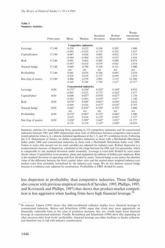
less dispersion in profitability than competitive industries. These findings
also concur with previous empirical research (Chevalier, 1995, Phillips, 1995,and Kovenock and Phillips, 1997) that shows that product-market competi-
tion is less aggressive when leading firms have high financial leverage.16
16 In contrast, Lipson (1993) shows that debt-coordinated collusion implies lower financial leverage inconcentrated industries. Bolton and Scharfstein (1990) argue that rivals prey more aggressively onfinancially vulnerable firms as the value of predation increases; this, too, would imply lower financialleverage in concentrated industries. Finally, Rotemberg and Scharfstein (1990) show that depending onwhat investors infer from rivals’ profitability, financial leverage can either facilitate or hinder collusion,and therefore rise or fall with industry concentration.
Table 1Summary statistics
Firm-years Mean MedianStandarddeviation
Robustdispersion
Range(maximum–minimum)
Competitive industriesLeverage 17,140 0.239 0.212 0.194 0.203 1.000
�0.005 �0.028 0.176 0.165 1.427Capital/Labor 17,140 0.047 0.024 0.085 0.022 1.375
�0.004 �0.004 0.078 0.015 4.164Risk 17,140 0.091 0.062 0.089 0.049 0.878
�0.007 �0.014 0.079 0.042 1.014Natural hedge 17,140 0.669 0.790 0.330 0.311 1.000
n/a n/a n/a n/a n/aProfitability 17,140 0.041 0.076 0.186 0.083 2.618
0.026 0.029 0.175 0.099 2.819Size (log of assets) 17,140 4.406 4.239 2.081 2.115 12.280
0.243 0.106 1.704 1.617 13.317
Concentrated industriesLeverage 1630 0.275a 0.256a 0.182a 0.169a 0.955
�0.005 �0.025 0.171c 0.163c 1.077Capital/labor 1630 0.048- 0.027a 0.070a 0.027c 1.170
�0.003 �0.005 0.058a 0.017- 1.180Risk 1630 0.074a 0.049a 0.081a 0.038a 0.632
�0.009 �0.010 0.071a 0.028a 0.795Natural hedge 1630 0.665- 0.810b 0.350a 0.352a 1.000
n/a n/a n/a n/a n/aProfitability 1630 0.072a 0.085a 0.135a 0.066a 1.940
0.015 0.016 0.128a 0.081a 1.737Size (log of assets) 1630 5.826a 5.599a 2.645a 3.051a 11.777
0.374 0.159 2.147a 2.094a 14.929
Summary statistics for manufacturing firms operating in 315 competitive industries and 46 concentratedindustries between 1981 and 2000. Superscripts show tests of differences between competitive and concen-trated industries where a, b, c denote statistical significance at the 1, 5, and 10% confidence levels. Followingthe U.S. Department of Justice, we define competitive industries as those with a Herfindahl–HirschmanIndex under 1000 and concentrated industries as those with a Herfindahl–Hirschman Index over 1800.Values in italics (the second row for each variable) are adjusted for industry-year. Robust dispersion is anonparametric measure of dispersion, calculated as the range between the 69th and 31st percentiles, whichis comparable to one standard deviation under normality. Leverage is total debt divided by total assets(book values). Capital/labor is net property, plant and equipment (in millions of dollars) per employee. Riskis the standard deviation of operating cash flow divided by assets. Natural hedge is one minus the absolutevalue of the difference between the firm’s capital–labor ratio and the market-share weighted industry-yearmedian (own firm excluded), normalized by the industry-year range. We do not demean natural hedgebecause it is industry-year adjusted by construction. Profitability is EBIT divided by assets.
The Review of Financial Studies / v 18 n 4 2005
1446
Our finding that financial structure, capital–labor ratios, and risk are
more dispersed within competitive industries is consistent with models of
perfect competition, where firm diversity arises endogenously within
competitive industries (Maksimovic and Zechner, 1991, Williams, 1995,
and Fries, Miller, and Perraudin, 1997) and models of imperfect competi-
tion, where dispersion decreases with industry concentration (Lipson,
1993, Lyandres, 2001). This finding also challenges the heuristic that
competition in competitive industries drives firms to similar financialstructure and cost structures.
In sum, we find that competitive and concentrated industries differ in
many important respects. The statistical and economic differences we find
in both the level and the dispersion of real and financial variables suggest
that industry structure reflects distinct equilibrium forces that lead to
diverse outcomes. These base results confirm that understanding the
effect of industry on firm decisions requires a richer treatment than
simply accounting for industry fixed effects.
3.3 Entry and exit in competitive and concentrated industries
To examine the dynamic predictions formulated by Williams (1995) and
Fries, Miller, and Perraudin (1997) for competitive industries, and by
Poitevin (1989) for concentrated industries, Table 2 presents subsample
means for entrants, incumbents, and exiters. Entrants are firms that
appear in the sample between 1991 and 2000 but not between 1981 and
1990. We distinguish these firms from those that enter an industry simplyby changing the nature of their operations (‘‘switchers’’). Exiters are firms
that appear in the sample between 1981 and 1990 period but not between
1991 and 2000. We distinguish these firms from those that leave an
industry through asset sales (‘‘sellers’’).17 Table 2 also reports subsample
means for the years following entry (‘‘post entry’’) and preceding exit
(‘‘pre-exit’’).
Several patterns emerge for competitive industries, both in industry-
year adjusted and unadjusted terms.18 First, entrants start off with highfinancial leverage ratios compared to incumbents, suggesting a greater
17 Data limitations prevent us from precisely determining the type of firm entry. For instance, we cannotdistinguish between privately-held incumbents that go public and new firms that actually add productivecapacity to their industry. We should point out that by tracking firms by their CRSP permanent number(permno) rather than by their COMPUSTAT CUSIP, we avoid miss-classifying firms that undergomergers and acquisitions or name changes as entrants. By using the historical SIC from CRSP ratherthan the current SIC from COMPUSTAT, we can identify incumbent firms that change industry. Thus,we refer to firms that change two-digit SIC industry between the 1981–1990 and 1991–2000 subperiods as"switchers". Finally, thanks to COMPUSTAT’s "reason for deletion" variable (note 35), we are able todistinguish between firms that exit through Chapter 11 bankruptcy or Chapter 7 liquidation and thosewhose assets are simply redeployed through corporate restructuring ("sellers").
18 Similar patterns appear in concentrated industries, however, most of the differences between the entrant,post entry, incumbent, pre exit, and exit categories are statistically insignificant because of the smallsample count.
Importance of Industry to Firm-Level Financial and Real Decisions
1447
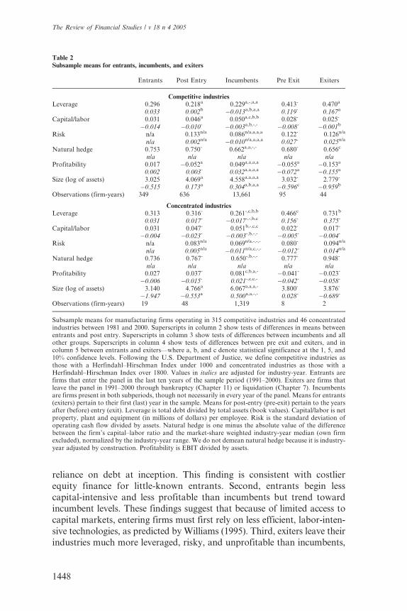
reliance on debt at inception. This finding is consistent with costlierequity finance for little-known entrants. Second, entrants begin less
capital-intensive and less profitable than incumbents but trend toward
incumbent levels. These findings suggest that because of limited access to
capital markets, entering firms must first rely on less efficient, labor-inten-
sive technologies, as predicted by Williams (1995). Third, exiters leave their
industries much more leveraged, risky, and unprofitable than incumbents,
Table 2Subsample means for entrants, incumbents, and exiters
Entrants Post Entry Incumbents Pre Exit Exiters
Competitive industriesLeverage 0.296 0.218a 0.229a,-,a,a 0.413- 0.470a
0.033 0.002b �0.013a,b,a,a 0.119- 0.167a
Capital/labor 0.031 0.046a 0.050a,c,b,b 0.028- 0.025-
�0.014 �0.010- �0.003a,b,-,- �0.008- �0.001b
Risk n/a 0.133n/a 0.086n/a,a,a,a 0.122- 0.126n/a
n/a 0.002n/a �0.010n/a,a,a,a 0.027- 0.025n/a
Natural hedge 0.753 0.750- 0.662a,a,-,- 0.680- 0.656c
n/a n/a n/a n/a n/aProfitability 0.017 �0.052a 0.049a,a,a,a �0.055a �0.153a
0.002 0.003- 0.032a,a,a,a �0.072a �0.155a
Size (log of assets) 3.025 4.069a 4.558a,a,a,a 3.032- 2.779-
�0.515 0.173a 0.304a,b,a,a �0.596c �0.959b
Observations (firm-years) 349 636 13,661 95 44
Concentrated industriesLeverage 0.313 0.316- 0.261-,c,b,b 0.466c 0.731b
0.031 0.017- �0.017-,-,b,c 0.156- 0.375-
Capital/labor 0.031 0.047- 0.051b,-,c,c 0.022- 0.017-
�0.004 �0.023- �0.003-,b,-,- �0.005- �0.004-
Risk n/a 0.083n/a 0.069n/a,-,-,- 0.080- 0.094n/a
n/a 0.005n/a �0.011n/a,c,-,- �0.012- 0.014n/a
Natural hedge 0.736 0.767- 0.650-,b,-,- 0.777- 0.948-
n/a n/a n/a n/a n/aProfitability 0.027 0.037- 0.081c,b,a,- �0.041- �0.023-
�0.006 �0.015- 0.021-,c,c,- �0.042- �0.058-
Size (log of assets) 3.140 4.766a 6.067a,a,a,- 3.800- 3.876-
�1.947 �0.553a 0.500a,a,-,- 0.028- �0.689-
Observations (firm-years) 19 48 1,319 8 2
Subsample means for manufacturing firms operating in 315 competitive industries and 46 concentratedindustries between 1981 and 2000. Superscripts in column 2 show tests of differences in means betweenentrants and post entry. Superscripts in column 3 show tests of differences between incumbents and allother groups. Superscripts in column 4 show tests of differences between pre exit and exiters, and incolumn 5 between entrants and exiters—where a, b, and c denote statistical significance at the 1, 5, and10% confidence levels. Following the U.S. Department of Justice, we define competitive industries asthose with a Herfindahl–Hirschman Index under 1000 and concentrated industries as those with aHerfindahl–Hirschman Index over 1800. Values in italics are adjusted for industry-year. Entrants arefirms that enter the panel in the last ten years of the sample period (1991–2000). Exiters are firms thatleave the panel in 1991–2000 through bankruptcy (Chapter 11) or liquidation (Chapter 7). Incumbentsare firms present in both subperiods, though not necessarily in every year of the panel. Means for entrants(exiters) pertain to their first (last) year in the sample. Means for post-entry (pre-exit) pertain to the yearsafter (before) entry (exit). Leverage is total debt divided by total assets (book values). Capital/labor is netproperty, plant and equipment (in millions of dollars) per employee. Risk is the standard deviation ofoperating cash flow divided by assets. Natural hedge is one minus the absolute value of the differencebetween the firm’s capital–labor ratio and the market-share weighted industry-year median (own firmexcluded), normalized by the industry-year range. We do not demean natural hedge because it is industry-year adjusted by construction. Profitability is EBIT divided by assets.
The Review of Financial Studies / v 18 n 4 2005
1448
consistent with received ideas on financial and economic distress. Lastly,
asset size and capital intensity rise and fall following entry and upon exit.
Fries, Miller, and Perraudin (1997) predict that, in competitive industries,
entrants are slightly less financially leveraged than incumbents and increase
their leverage ratios following entry; our findings support neither of these
predictions—in fact, we find just the opposite. While we do find that entrants
are less capital intensive than incumbents, our evidence does not support
Williams’ (1995) prediction that entrants begin their existence substantiallyless financially leveraged than incumbents.However, our finding that entrants
start offwith high financial leverage ratios does fit Poitevin’s (1989) prediction
that ‘‘high-value’’ entrants issue debt to signal type and enter the industry with
a high level of financial leverage relative to incumbents.
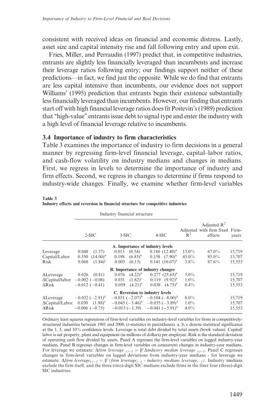
3.4 Importance of industry to firm characteristics
Table 3 examines the importance of industry to firm decisions in a general
manner by regressing firm-level financial leverage, capital–labor ratios,
and cash-flow volatility on industry medians and changes in medians.
First, we regress in levels to determine the importance of industry and
firm effects. Second, we regress in changes to determine if firms respond toindustry-wide changes. Finally, we examine whether firm-level variables
Table 3Industry effects and reversion in financial structure for competitive industries
Industry financial structure
2-SIC 3-SIC 4-SICAdjusted
R2
Adjusted R2
with firm fixedeffects
Firm-years
A. Importance of industry levelsLeverage 0.048 (1.37) 0.013 (0.54) 0.186 (12.40)a 13.0% 67.0% 15,719Capital/Labor 0.350 (14.00)a 0.198 (6.83)a 0.158 (7.90)a 45.0% 85.0% 15,707Risk 0.068 (1.84)c 0.003 (0.13) 0.141 (10.07)a 3.8% 87.6% 15,553
B. Importance of industry changesDLeverage 0.026 (0.81) 0.076 (4.22)a 0.277 (25.65)a 5.0% 15,719DCapital/labor �0.002 (�0.08) 0.031 (1.82)c 0.119 (9.92)a 1.0% 15,707DRisk �0.012 (�0.41) 0.059 (4.21)a 0.038 (4.75)a 0.4% 15,553
C. Reversion to industry levelsDLeverage �0.032 (�2.91)a �0.031 (�2.07)b �0.104 (�8.00)a 8.0% 15,719DCapital/Labor 0.030 (1.88)c �0.045 (�3.46)a �0.035 (�3.89)a 1.0% 15,707DRisk �0.006 (�0.75) �0.013 (�1.39) �0.041 (�5.91)a 4.0% 15,553
Ordinary least squares regressions of firm-level variables on industry-level variables for firms in competitively-structured industries between 1981 and 2000. (t-statistics in parentheses). a, b, c denote statistical significanceat the 1, 5, and 10% confidence levels. Leverage is total debt divided by total assets (book values). Capital/labor is net property, plant and equipment (in millions of dollars) per employee. Risk is the standard deviationof operating cash flow divided by assets. Panel A regresses the firm-level variables on lagged industry-yearmedians. Panel B regresses changes in firm-level variables on concurrent changes in industry-year medians.For leverage we estimate: Dfirm leverage t,t�1 ¼ b�Dindustry median leverage t,t�1. Panel C regresseschanges in firm-level variables on lagged deviations from industry-year medians - for leverage weestimate: Dfirm leveraget,t�1 ¼ b�(firm leveraget�1 - industry medians leveraget�1). Industry mediansexclude the firm itself, and the three (two)-digit SIC medians exclude firms in the finer four (three)-digitSIC industries.
Importance of Industry to Firm-Level Financial and Real Decisions
1449
revert back to industry benchmarks by regressing changes in firm charac-
teristics on lagged firm-level deviations from industry medians.
The industry fixed effects in Table 3 are nested in the sense that firms
and industries used in narrowly-defined industry medians are excluded
from the calculation of more broadly-defined industry medians. For
instance, median four-digit SIC industry financial leverage for a given
firm in SIC 3561 excludes that firm. Median three-digit SIC industry
financial leverage for all firms in SIC 3561 excludes these firms butincludes all other firms in the 356 SIC. Finally, median two-digit SIC
industry financial leverage for all firms in SIC 356 excludes these firms
but includes all other firms in the 35 SIC.19 We only analyze competitive
industries because the distinction between ‘‘firm’’ and ‘‘industry’’ is lost if
each firm represents a significant part of the industry itself.
Panel A regresses the firm-level variables on lagged industry-year med-
ian levels, first without firm fixed effects (reported coefficients), then
including firm fixed effects. We lag the industry medians to avoid endo-geneity problems.20 This is essentially an analysis of variance where the
adjusted R-square indicates the importance of industry in explaining
firm-level characteristics. We find that industry is relatively unimportant
in explaining firm financial structure, at least in our sample of competitive
manufacturing industries, where the adjusted R-square is only 13%. The
adjusted R-square rises sharply if we add firm fixed effects (67%), which
shows that most of the variation in financial leverage arises within indus-
tries rather than between industries.21
In contrast, industry effects explain much of the variation in capital–
labor ratios (45%). Firm fixed effects explain another 40% of the variation
in capital–labor ratios while 15% is within-firm. This shows that capital
intensity is highly industry-specific, with some variation across firms
within industries but little firm-level change over time. These findings
are consistent with capital intensity being essentially fixed once technol-
ogy is chosen. They also suggest that industry dummies are reasonable
proxies for capital intensity. Finally, industry explains little of the varia-tion in cash-flow volatility (4%), most of it being within-industry.
Together, these findings make the strong but simple case that firms in
a given industry differ widely with respect to their real and financial
characteristics.
19 This causes the degrees of freedom to drop from the 17,140 observations reported in Table 1. This isbecause some three-digit SIC industries contain a single four-digit SIC industry.
20 The adjusted R-squares only increase about two percentage points if we use contemporaneous industrymedians.
21 Bradley, Jarrell, and Kim (1984) regress firms’ average debt ratios for 1962-1981 on two-digit SICdummies for a broad set of industries. They report that industry fixed effects explain 23.6% of thevariation in financial structure. We examine firms in a time-panel of manufacturing industries (not panelaverages), and over a different time period, which explains why our R-square is somewhat lower thantheirs.
The Review of Financial Studies / v 18 n 4 2005
1450
Panel B examines how firms respond to industry-wide changes by
regressing changes in firm-level variables on concurrent changes in
industry-year medians. Although we find statistical significance, the low
R-squares (5% and under) and point estimates that are far away from one
suggest that firms adjust their financial structures little in response to
overall industry trends.22 Similar results obtain for capital–labor ratios
and cash-flow volatility. We conclude that changes in firm characteristics
bear a small to moderate relation to industry-level changes.Finally, we consider whether the observed diversity within industries
reverses over time by investigating whether firms drift back to their
industry medians. Panel C examines this question by regressing changes
in firm characteristics on lagged firm-level deviations from industry-year
medians. We find that firms do revert to industry norms, though very
slowly. We find annual financial-leverage industry-median reversion rates
of 3.2% for two-digit, 3.1% for three-digit, and 10.4% for four-digit
industries, not unlike Fama and French (2002) who report that firmsrevert to their own leverage targets at rates of 7% to 18% per year. This
evidence of slow reversion is consistent with Fischer, Heinkel, and Zechner
(1989) in suggesting that there are substantial transaction costs in adjusting
firm financial structure. However, it is also consistent with industry equili-
brium outcomes where firms do not trend toward the industry norm but
rather adopt differential finance-technology-risk configurations that persist
over time. Since slow industry reversion could equally reflect transaction
costs or equilibrium forces, we next look more closely at how firms evolvewithin their industries.
3.5 Evolution of entrants, exiters, switchers, sellers, and incumbents
within industries
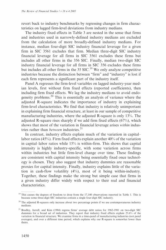
To expand on our findings of Table 3 and investigate the dynamic proper-
ties of the competitive-industry equilibrium models (Williams, 1995, and
Fries, Miller, and Perraudin, 1997), Table 4 presents transition frequen-
cies for firms that enter, stay, or leave their industries. For each variablepresented, the table panels show the percentage of incumbent firms that
stay in the same industry-year quintile or move to other quintiles between
the first half of the empirical period (1981–1990) and the second half
(1990–2000). Each panel also shows the 1990–2000 quintile distribution
of firms that enter an industry in the 1990–2000 time period, either
through new entry (enter) or by changing two-digit SIC industry (switch).
Finally, the panels show the 1981–1990 quintile distribution of firms that
leave an industry in the 1990–2000 time period, either through bank-ruptcy or liquidation (exit) or by selling assets through corporate mergers
22 This finding is consistent with Roberts (2002) who reports that firms do not adjust their financialstructure to industry targets, but rather adjust to a firm-specific target financial structure.
Importance of Industry to Firm-Level Financial and Real Decisions
1451
Table 4Transition frequencies for competitive industries
Firm status in 1991–2000
Q1 Q2 Q3 Q4 Q5 Exit Sell Total
LeverageEnter 25 18 18 20 18b 17-
Switch 12 19 21 25 23a 11b
Q1 32a 18 9 4 2 3 32 10a
Q2 10 28a 19 9 3 1 30 18a
Q3 4 17 22a 18 7 2 32 17a
Q4 2 9 17 23a 15 4 31 17a
Q5 1 5 7 17 30a 9a 31- 12a
Total 11 17 17 17 13 3a 22a 100
Capital/LaborEnter 14 22 22 21 22b 17c
Switch 19 25 23 15 18- 11-
Q1 30a 21 5 0 0 8 36 10a
Q2 12 27a 15 7 1 3 35 17a
Q3 5 19 21a 14 5 3 33 16a
Q4 2 8 18 29a 13 2 27 17a
Q5 2 2 11 28 32a 3- 23- 12a
Total 11 18 17 17 13 3- 22a 100
RiskEnter 18 19 20 23 20- 17-
Switch 13 21 21 27 18- 11b
Q1 30a 27 11 5 0 0 27 10a
Q2 16 29a 17 8 2 1 27 17a
Q3 6 18 19a 18 3 4 32 17a
Q4 3 9 18 24a 8 5 33 17a
Q5 0 3 10 16 28a 8a 35b 11a
Total 12 18 17 17 11 3a 22a 100
Natural hedgeEnter 16 20 19 23 22c 17-
Switch 18 15 19 25 22- 11-
Q1 33a 23 8 1 2 5 27 10a
Q2 12 30a 16 8 2 3 30 17a
Q3 5 18 24a 15 4 2 32 16a
Q4 2 7 16 28a 12 3 32 17a
Q5 0 1 8 20 31a 6- 33b 12a
Total 11 17 17 18 13 3- 22a 100
ProfitabilityEnter 21 21 20 20 18- 17-
Switch 17 24 20 24 15- 11-
Q1 17a 19 6 6 3 12 36 10a
Q2 12 23a 16 11 5 4 29 17a
Q3 6 17 22a 16 7 2 30 17a
Q4 2 10 18 23a 14 2 31 17a
Q5 2 7 14 18 28a 0a 31- 12a
Total 11 17 17 17 13 3a 22b 100
Size (log of assets)Enter 12 17 25 28 18b 17a
Switch 19 30 19 16 16- 11a
Q1 36a 18 3 0 0 8 34 9a
Q2 13 26a 15 3 1 4 38 17a
The Review of Financial Studies / v 18 n 4 2005
1452
or acquisitions (sell). The quintiles are formed using firm means for each
time period (1981–1990 and 1990–2000). The table also reports statisticaltests of differences in proportions between quintiles and goodness-of-fit
tests that industry transition patterns follow a uniform distribution. As in
Table 3, we only run this analysis for competitive industries.
We note several transition patterns for incumbent firms and for firms
that enter or leave their industries. First, the top-left panel of Table 4 shows
that 25% of entrants fall in the lowest financial-leverage quintile. This
percentage is a significantly lower 18% in quintile five. In contrast, switchers
tend to enter an industry in the higher financial-leverage quintiles, with 23%(12%) of switchers in the fifth (first) quintile. Among exiters, three times
more firms belong to the top financial-leverage quintile than the bottom
quintile. This pattern does not obtain for sellers, where firms are roughly
equally distributed across financial-leverage quintiles. Since most of the
transition frequencies pertaining to entrants, switchers, sellers, and exiters
concur with the Section 3.3 discussion of firmmeans reported in Table 2, we
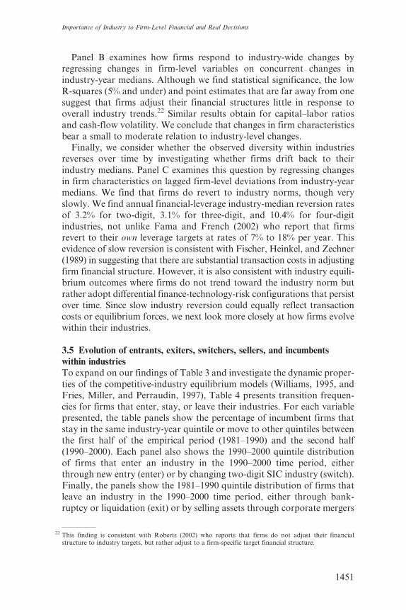
now turn our attention to the behavior of incumbent firms over time.
The diagonal elements of each panel represent incumbent persistencerates, namely, the percentage of firms that remain in their industry
quintile between the period 1981–1990 and the period 1990–2000. For
all variables, we find that persistence is greatest for quintiles one, five, or
both. This may simply reflect the fact that these quintiles contain the tails
of the distribution for each variable: Firms in these quintiles must change
substantially to transit to the inner quintiles. The highest persistence
rates are 32, 31, and 51% for the fifth quintiles for capital–labor ratios,
natural hedge, and asset size, and 36, 33, and 32% for the first asset-size,
Table 4(continued)
Firm status in 1991–2000
Q1 Q2 Q3 Q4 Q5 Exit Sell Total
Q3 5 19 26a 10 2 3 35 17a
Q4 1 7 19 35a 11 2 25 18a
Q5 0 1 3 22 51a 2a 22- 12a
Total 11 17 17 17 13 3c 22a 100
Quintile transition frequencies for firm-period means between 1981–1990 and 1991–2000 for firms thatenter or switch industries, incumbents, and firms that leave the panel through exit or sale. Each panelshows percentages relative to row totals. Superscripts in the last column and bottom row of each panelshow Chi-square tests that industry demographics follow a uniform distribution. Superscripts in quintilefive test whether the percentages in quintiles one and five are equal. Superscripts on the diagonal quintilestest whether adjacent quintiles are equal. a, b, c denote statistical significance at the 1, 5, and 10%confidence levels. Leverage is total debt divided by total assets (book values). Capital/labor is netproperty, plant and equipment (in millions of dollars) per employee. Risk is the standard deviation ofoperating cash flow divided by assets. Natural hedge is one minus the absolute value of the differencebetween the firm’s capital–labor ratio and the market-share weighted industry-year median (own firmexcluded), normalized by the industry-year range. Profitability is EBIT divided by assets.
Importance of Industry to Firm-Level Financial and Real Decisions
1453
natural-hedge, and leverage quintiles. These results suggest that large, capital-
intensive, profitable, and stable incumbent firms tend to maintain their
dominant industry position over time and represent aWilliams-style industry
core. Higher turnover rates and lower persistence rates arise as capital
intensity, profitability, and asset size decrease and as financial leverage and
cash-flow volatility increase. These results suggest that small, labor-intensive,
unprofitable, risky, marginal firms tend to move in, around, and out of their
industries over time and represent a Williams-style industry fringe.For all variables, we find persistence rates that significantly diverge
from 20%, the rate expected if incumbents were uniformly randomly
redistributed across quintiles between 1981–1990 and the 1990–2000
time period.23 Consistent with our industry-median reversion analysis
(Table 3), this finding suggests that firm characteristics evolve slowly
and that firms maintain their relative industry position, even within
competitively-structured industries. Table 4 also highlights the high attri-
tion rate among small firms (fully 34% of firms in the lowest asset-sizequintile sell out, 8% exit, and 36% remain in the lowest asset-size quintile)
and the staying power of large firms (51% of firms in the highest asset-size
quintile remain in that quintile, 2% exit, and 22% sell out).
What Tables 3 and 4 demonstrate is that the traditional, fixed-effects
view of industry is of limited use in explaining firm financial structure.
Yet, we find high persistence in incumbents’ industry position along real
and financial dimensions, suggesting that, as recent theories contend,
industry equilibrium forces may act to sustain intra-industry diversityrather than smooth it away. An alternative explanation is that the
observed diversity reflects firm-level hysteresis caused by transaction
costs and financial constraints. While such frictions might explain persis-
tence in the absolute level of firm characteristics, it cannot account for the
persistence in a firm’s industry ranking unless we (unrealistically) assume
that all firms in an industry share very similar adjustment paths.
3.6 Multivariate analysisAlthough informative, the evidence uncovered so far on the role of
industry factors relies on univariate analyses. In this section, we investigate
whether this evidence holds up in a simultaneous-equation instrumental-
variable estimation framework that deals with endogeneity in the regressors
and simultaneity between three dependent variables featured in the industry
equilibrium models: financial leverage, capital–labor ratios, and cash-flow
volatility.
23 True persistence rates are even higher because the percentages shown are relative to all firms, not justincumbents. For a narrower test of persistence, we test whether the percentage of incumbents that remainin the same quintile is different than the percentage of incumbents that move up or down one quintile. Forevery quintile and for every variable, we reject the null hypothesis that these percentages are equal at the1% confidence level or better.
The Review of Financial Studies / v 18 n 4 2005
1454
3.6.1 Econometric Approach. Table 5 presents OLS and GMM regres-
sion results for competitive industries. In contrast to OLS, GMM allows
for simultaneity among the dependent variables by incorporating the
correlation of residuals across the three equations. This improves the
efficiency and consistency of the estimates. As an instrumental-variableestimation method, GMM also mitigates simultaneity bias.24 However,
we also present OLS results for comparison with prior work that uses
non-IV methods (e.g., Titman and Wessels, 1988, Rajan and Zingales,
1995, Barclay, Morellec, and Smith, 2003).
For our GMM regressions, we instrument all variables except for the
entry/exit dummy variables and the quantile changes by their second lags
in levels. The instrument set includes the four dummy variables (enter,
switch, sell, and exit), current and lagged intra- and extra-quantilechanges for the three dependent variables (twelve variables), and a con-
stant term, resulting in ten over-identifying restrictions per equation.
We use Hansen’s (1982) J-statistic to jointly test whether the model is
well-specified and the instruments are valid, that is, uncorrelated with the
residuals. Except for the risk equation, Table 5 shows that the over-
identifying restrictions are not rejected at conventional statistical levels,
indicating that the financial leverage and capital–labor equations are well-
specified and that the instrument set is valid, that is, that the instrumentsare sufficiently orthogonal to the residuals.
The instruments must also be relevant, that is, correlated with the
endogenous variables. We test the relevance of the instrument set using
the procedure outlined in Shea (1997) for multivariate models.25 Table 5
shows instrument relevance values of about 8% for financial leverage,
10% for capital–labor, and 18% for risk. Although there is no accepted
norm on what constitutes a relevant set of instruments, these values
(interpretable as R-squares) are statistically significant and consistentwith the level of explanatory power generally found in corporate finance
studies.26
24 Despite these advantages over OLS, Ferson and Foerster (1994) show that GMM can understate thecoefficient standard errors. They find that this problem mainly arises in the small samples they study(60 observations) and tends to vanish as their sample size grows to 720 observations.
25 First, regress each endogenous variable on the set of instruments; save the fitted values. Second, regresseach endogenous variable on the remaining endogenous variables; save the residuals. Third, regress eachfitted endogenous variable on the remaining fitted endogenous variables; save the residuals. Fourth,regress the residuals from the second step on the residuals from the third step; save the R-squares. Finally,adjust the R-squares for the number of observations and instruments. These R-squares are reported at thebottom of Table 5.
26 We experimented with several other sets of instruments, such as adding the third lags in levels, the firstand second leading values in levels (as suggested by Hayashi and Inoue, 1991), or the squared and cubedvalues of the second lags in levels, none of which materially improved the relevance measures without alsocausing a rejection of the over-identifying restrictions or a substantial drop in sample size. Another reasonto limit the number of instruments is that, as Angrist and Krueger (2001) discuss, adding weak instru-ments (poorly correlated to the endogenous variables) can bias IV estimates and this bias increases inproportion to the number of over-identifying restrictions.
Importance of Industry to Firm-Level Financial and Real Decisions
1455
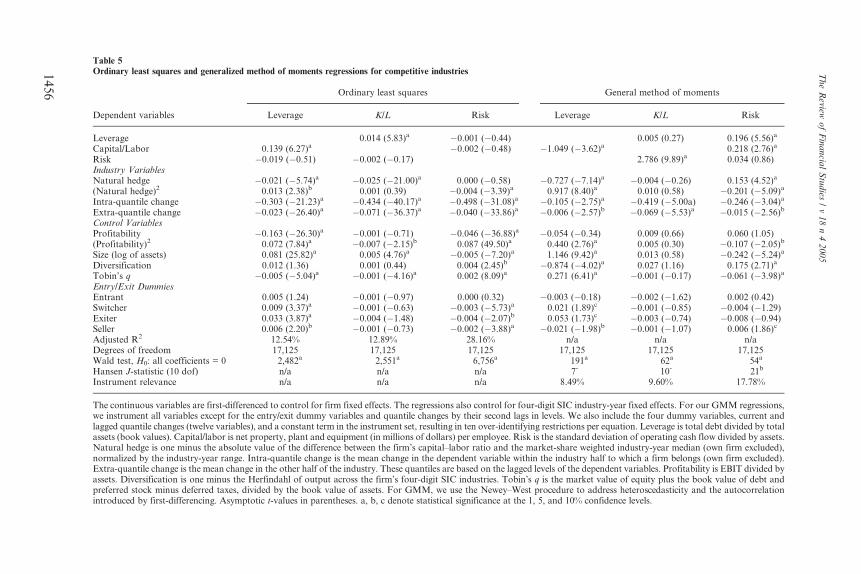
Table 5Ordinary least squares and generalized method of moments regressions for competitive industries
Ordinary least squares General method of moments
Dependent variables Leverage K/L Risk Leverage K/L Risk
Leverage 0.014 (5.83)a �0.001 (�0.44) 0.005 (0.27) 0.196 (5.56)a
Capital/Labor 0.139 (6.27)a �0.002 (�0.48) �1.049 (�3.62)a 0.218 (2.76)a
Risk �0.019 (�0.51) �0.002 (�0.17) 2.786 (9.89)a 0.034 (0.86)Industry VariablesNatural hedge �0.021 (�5.74)a �0.025 (�21.00)a 0.000 (�0.58) �0.727 (�7.14)a �0.004 (�0.26) 0.153 (4.52)a
(Natural hedge)2 0.013 (2.38)b 0.001 (0.39) �0.004 (�3.39)a 0.917 (8.40)a 0.010 (0.58) �0.201 (�5.09)a
Intra-quantile change �0.303 (�21.23)a �0.434 (�40.17)a �0.498 (�31.08)a �0.105 (�2.75)a �0.419 (�5.00a) �0.246 (�3.04)a
Extra-quantile change �0.023 (�26.40)a �0.071 (�36.37)a �0.040 (�33.86)a �0.006 (�2.57)b �0.069 (�5.53)a �0.015 (�2.56)b
Control VariablesProfitability �0.163 (�26.30)a �0.001 (�0.71) �0.046 (�36.88)a �0.054 (�0.34) 0.009 (0.66) 0.060 (1.05)(Profitability)2 0.072 (7.84)a �0.007 (�2.15)b 0.087 (49.50)a 0.440 (2.76)a 0.005 (0.30) �0.107 (�2.05)b
Size (log of assets) 0.081 (25.82)a 0.005 (4.76)a �0.005 (�7.20)a 1.146 (9.42)a 0.013 (0.58) �0.242 (�5.24)a
Diversification 0.012 (1.36) 0.001 (0.44) 0.004 (2.45)b �0.874 (�4.02)a 0.027 (1.16) 0.175 (2.71)a
Tobin’s q �0.005 (�5.04)a �0.001 (�4.16)a 0.002 (8.09)a 0.271 (6.41)a �0.001 (�0.17) �0.061 (�3.98)a
Entry/Exit DummiesEntrant 0.005 (1.24) �0.001 (�0.97) 0.000 (0.32) �0.003 (�0.18) �0.002 (�1.62) 0.002 (0.42)Switcher 0.009 (3.37)a �0.001 (�0.63) �0.003 (�5.73)a 0.021 (1.89)c �0.001 (�0.85) �0.004 (�1.29)Exiter 0.033 (3.87)a �0.004 (�1.48) �0.004 (�2.07)b 0.053 (1.73)c �0.003 (�0.74) �0.008 (�0.94)Seller 0.006 (2.20)b �0.001 (�0.73) �0.002 (�3.88)a �0.021 (�1.98)b �0.001 (�1.07) 0.006 (1.86)c
Adjusted R2 12.54% 12.89% 28.16% n/a n/a n/aDegrees of freedom 17,125 17,125 17,125 17,125 17,125 17,125Wald test, H0: all coefficients = 0 2,482a 2,551a 6,756a 191a 62a 54a
Hansen J-statistic (10 dof) n/a n/a n/a 7- 10- 21b
Instrument relevance n/a n/a n/a 8.49% 9.60% 17.78%
The continuous variables are first-differenced to control for firm fixed effects. The regressions also control for four-digit SIC industry-year fixed effects. For our GMM regressions,we instrument all variables except for the entry/exit dummy variables and quantile changes by their second lags in levels. We also include the four dummy variables, current andlagged quantile changes (twelve variables), and a constant term in the instrument set, resulting in ten over-identifying restrictions per equation. Leverage is total debt divided by totalassets (book values). Capital/labor is net property, plant and equipment (in millions of dollars) per employee. Risk is the standard deviation of operating cash flow divided by assets.Natural hedge is one minus the absolute value of the difference between the firm’s capital–labor ratio and the market-share weighted industry-year median (own firm excluded),normalized by the industry-year range. Intra-quantile change is the mean change in the dependent variable within the industry half to which a firm belongs (own firm excluded).Extra-quantile change is the mean change in the other half of the industry. These quantiles are based on the lagged levels of the dependent variables. Profitability is EBIT divided byassets. Diversification is one minus the Herfindahl of output across the firm’s four-digit SIC industries. Tobin’s q is the market value of equity plus the book value of debt andpreferred stock minus deferred taxes, divided by the book value of assets. For GMM, we use the Newey–West procedure to address heteroscedasticity and the autocorrelationintroduced by first-differencing. Asymptotic t-values in parentheses. a, b, c denote statistical significance at the 1, 5, and 10% confidence levels.
TheReview
ofFinancia
lStudies
/v18n42005
1456
The panel nature of our sample allows us to control for unobserved firm-
specific factors. Instead of the usual deviation-from-means approach,
which is invalid when using lagged variables as instruments, we control
for firm fixed effects by first-differencing the variables. However, first-
differencing introduces first-order moving-average autocorrelation. Our
GMM estimation uses the Newey–West (Newey and West, 1987) proce-
dure to address this issue and adjust for heteroscedasticity. We also include
four-digit SIC interacted industry-year fixed effects to focus on variationwithin industries.
3.6.2 Regression results. Table 5 shows several differences between the
OLS and GMM coefficient estimates. Several of the coefficient signs
change as we go from OLS, which uses realized values of the variables,
to GMM, which uses predicted (instrumented) values of the variables.
For instance, we find that the relation between financial leverage and the
capital–labor ratio is positive and significant for OLS but negative andsignificant for GMM.27,28 The coefficient signs for risk and Tobin’s q also
change across the two estimation methods. These differences show that
the simultaneity of financial leverage and its determinants is a real con-
cern requiring proper econometric treatment. Since the GMM estimates
address this issue directly, inasmuch as the chosen instrument set is both
valid and relevant, we emphasize the GMM results over the OLS esti-
mates. In any case, results for the industry position variables—natural
hedge and intra- and extra-quantile change—are similar across estimationmethods.
The first industry position variable we examine is a firm’s natural
hedge, which measures how close a firm’s capital–labor ratio is to the
industry-year median. We find a significant inverse relation between this
variable and financial leverage, supporting Maksimovic and Zechner’s
(1991) prediction that firms that depart from the median industry tech-
nology choose high financial leverage.
27 We have traced the cause of this sign switch to an endogeneity problem in the OLS estimation. Wehypothesized that the relation between financial leverage and the capital-labor ratio reflects two offsettingfactors: a collateral effect (more fixed capital, more debt capacity) and a substitution effect (moreoperating leverage, less financial leverage). As an indirect test of the collateral effect, we drop asset sizefrom the model. We find that this has no qualitative effect on the capital-labor coefficient in the OLSestimation but changes the sign from negative to positive in the GMM estimation, confirming that assetsize and the capital-labor ratio are interdependent. As a more direct proxy of the collateral effect, we addthe capital-to-assets ratio to the model (along with assets). Doing so lowers the statistical significance ofcapital-labor in the OLS but raises its statistical significance in the GMM estimation. Thus, we concludethat as an IV estimator that addresses simultaneity bias by using predicted rather than realized values ofendogenous variables, GMM does a better job than OLS in picking up both the collateral effect (throughassets) and the substitution effect (through instrumented capital-labor ratios).
28 The interacted industry-year fixed effects are also key to having GMM pick up this substitution effect,since without them the coefficient on the capital-labor ratio in the financial leverage GMM regression isinsignificant.
Importance of Industry to Firm-Level Financial and Real Decisions
1457
We also include two other industry position variables to capture the
central idea that, even in competitive industries, decisions made by indi-
vidual firms are related to the decisions made by other firms in their
industry. We include the change in financial structure, technology, and
risk of industry firms both above and below the industry median. For
instance, if a firm’s financial leverage is less than or equal to the median
financial leverage for its industry-year, then we define ‘‘intra-quantile
change’’ as the mean change in financial leverage of all other firmswhose financial leverage is less than or equal to the median for that
particular industry and year; ‘‘extra-quantile change’’ is the mean change
in financial leverage of all firms above the median in that industry-year.
A similar procedure is used for firms whose financial leverage lies above
the industry-year median. The same is done for the other two dependent
variables (capital–labor ratios and cash-flow volatility).
Regardless of estimation method (OLS or GMM), we find negative
and significant coefficients for these intra- and extra-quantile changes ineach of the three equations we consider. In other words, we find that
changes in own-firm financial leverage, capital-intensity, and cash-flow
volatility are inversely related to changes made by other firms within the
same industry. This finding supports the asymmetric adjustment patterns
predicted by Maksimovic and Zechner (1991) where the equilibrium
process drives firms to react differently to common industry shocks.
These relations are stronger (weaker) inside (outside) a firm’s industry-
year quantile, indicating that firms pay most attention to industry peerswith similar characteristics. Thus, we conclude that firm interdependence,
usually associated with imperfect competition, arises even within
competitively-structured industries.
Maksimovic and Zechner also show how debt, technology, and risk are
jointly determined, which motivates our use of simultaneous equation
methods. Our results confirm that this approach is justified as capital-
intensity and cash-flow volatility explain financial leverage, and financial
leverage and capital-intensity explain cash-flow volatility. However, cau-sation does not run both ways: We find no significant relation between
capital-intensity and financial leverage or cash-flow volatility.
Our GMM results show that firms with riskier cash flows tend to use
more financial leverage. This finding is of particular interest since past
empirical work has in turn found the relation between financial leverage
and cash-flow volatility to be positive (Kim and Sorensen, 1986), negative
(Bradley, Jarrell, and Kim, 1984), and insignificant (Titman and Wessels,
1988). Besides lending credence to Maksimovic and Zechner’s (1991)prediction of a positive relation between financial leverage and risk, this
finding also suggests that the mixed results in the literature might depend
on the econometric treatment of simultaneous decision variables and
endogenous explanatory variables.
The Review of Financial Studies / v 18 n 4 2005
1458
Our regressions include squared values for natural hedge and profit-
ability because an unreported analysis of how variables distribute across
industry quintiles shows significant non-monotonic relations between
these variables and the dependent variables. We find a significant positive
coefficient for the squared value of natural hedge, indicating a U-shaped
relation between this variable and financial leverage. This non-monotonic
relation is not predicted by Maksimovic and Zechner (1991) and suggests
that factors besides those analyzed in their model induce firms at thetechnological core of the industry to assume more debt than firms whose
capital–labor ratios lie between the core and fringe of the industry. How-
ever, as we show next (Table 6), the combined impact of the squared and
unsquared values of natural hedge is negative, as per their prediction.29
One possibility is that our natural hedge measure acts as a proxy for
financial distress. As shown in Table 2, we observe a drop in capital
intensity in years prior to exit, causing natural hedge to drop as well
(although neither of these variables differ significantly from incumbentlevels once we adjust for industry-year). We use two methods to avoid
confusing financial distress with a bona fide natural-hedge effect. First, we
include (instrumented) capital–labor ratios themselves in the financial
leverage regressions; we also control for risk, profitability, and size,
which Table 2 showed to correlate with financial distress and exit. Sec-
ond, we include dummy variables for exiting firms.
Since our univariate results showed significant differences between
firms that enter, stay, or leave their industries, our regressions alsoinclude indicator variables for entrants, switchers, sellers, and exiters
(incumbents are the omitted category). These dummy variables allow us
to contrast Maksimovic and Zechner’s (1991) static industry equilibrium
model, where entry and exit play no role because the number of firms in
the industry is held constant, and dynamic industry equilibrium models
by Williams (1995) and Fries, Miller, and Perraudin (1997), where entry
and exit are endogenized.
Table 2 showed that entering and exiting firms carry more leveragethan incumbents. However, our multivariate results show that only firms
that switch into an industry or exit through bankruptcy or liquidation
carry significantly more leverage than incumbents. Our GMM regressions
also show no evidence that entrants or exiters differ from incumbents in
terms of capital-intensity or cash-flow volatility.30 Thus, we find no
multivariate evidence to support the Williams (1995) and Fries, Miller,
and Perraudin’s (1997) prediction that entrants carry less debt than
incumbents.
29 Excluding the squared term from the regressions does not change this conclusion.
30 Firms that exit by selling assets are statistically riskier, although only at the 10% confidence level.
Importance of Industry to Firm-Level Financial and Real Decisions
1459
As an indirect test and benchmark for our results, we run the same
regressions for the sample of concentrated industries presented earlier
(Tables 1 and 2). We do so to examine whether the measures of a firm’s
industry position we develop to test competitive-industry equilibrium mod-
els also help explain firm financial structure in concentrated industries. If
these variables are also significant for concentrated industries, then we
would conclude that the forces modeled in the context of competitive-
industry equilibrium extend to concentrated industries. Otherwise, wewould conclude that the forces captured in these models are indeed specific
to competitive industries. Since this is essentially a robustness check, we do
not present regressions for the concentrated industry sample.
Comparing GMM results across industry types, we find that most of
the variables that are statistically significant determinants of financial
leverage and cash-flow volatility in competitive industries are not signifi-
cant in concentrated industries. Focusing on the industry position vari-
ables, we find that none of the natural hedge or entry/exit dummyvariables are significant in concentrated industries. However, changes
inside and outside a firm’s industry-year quantile continue to be highly
significant for all three dependent variables. As we later show, these
variables are also more economically significant in concentrated indus-
tries than they are in competitive industries.
To summarize, regardless of estimation method (OLS or GMM), we find
empirical evidence consistent with many of the predictions deriving from
the static industry equilibriummodel presented inMaksimovic and Zechner(1991). For instance, we find an inverse relation between financial leverage
and natural hedge. We also find that firms tend to adjust away from their
industry peers. In contrast, we find no multivariate support for the predic-
tions deriving from the dynamic industry equilibrium models presented by
Williams (1995) and Fries, Miller, and Perraudin (1997).
3.6.3 Economic significance. Table 6 reports the economic significance of
our multivariate regression results. The table presents predicted percentagechanges in the dependent variables as each regressor varies from the 25th to
75th percentile, holding all other regressors at their sample mean levels (sta-
tistically insignificant relations are omitted). The percentages we report are
relative to themeanandarenormalizedby the sample range (maximumminus
minimum). The top (bottom) panel pertains to competitive (concentrated)
industries. Both panels use the GMM regression coefficient estimates.31
31 Because the GMM coefficient estimates are obtained from predicted (instrumented) values of thevariables rather than their realized values, we compute economic significance using predicted ratherthan realized values of the variables. The economic impact that natural hedge and profitability have onfinancial leverage is complicated by the non-monotonic relations between these variables and financialleverage. Indeed, Table 5 shows negative coefficients for both variables and positive coefficients for theirsquared values. Table 6 combines these offsetting relations and presents the total effect each of thesevariables has on the dependent variables.
The Review of Financial Studies / v 18 n 4 2005
1460
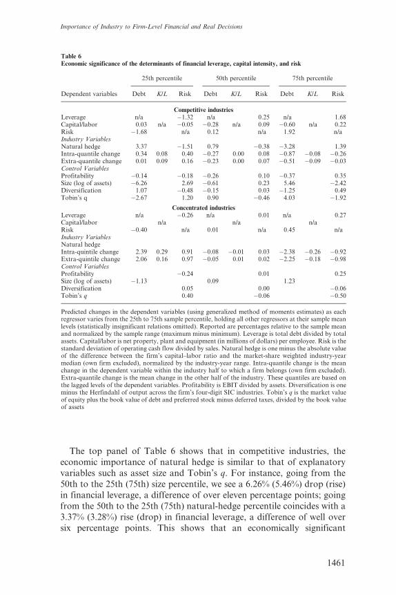
The top panel of Table 6 shows that in competitive industries, the
economic importance of natural hedge is similar to that of explanatory
variables such as asset size and Tobin’s q. For instance, going from the
50th to the 25th (75th) size percentile, we see a 6.26% (5.46%) drop (rise)
in financial leverage, a difference of over eleven percentage points; going
from the 50th to the 25th (75th) natural-hedge percentile coincides with a
3.37% (3.28%) rise (drop) in financial leverage, a difference of well oversix percentage points. This shows that an economically significant
Table 6Economic significance of the determinants of financial leverage, capital intensity, and risk
25th percentile 50th percentile 75th percentile
Dependent variables Debt K/L Risk Debt K/L Risk Debt K/L Risk
Competitive industriesLeverage n/a �1.32 n/a 0.25 n/a 1.68Capital/labor 0.03 n/a �0.05 �0.28 n/a 0.09 �0.60 n/a 0.22Risk �1.68 n/a 0.12 n/a 1.92 n/aIndustry VariablesNatural hedge 3.37 �1.51 0.79 �0.38 �3.28 1.39Intra-quantile change 0.34 0.08 0.40 �0.27 0.00 0.08 �0.87 �0.08 �0.26Extra-quantile change 0.01 0.09 0.16 �0.23 0.00 0.07 �0.51 �0.09 �0.03Control VariablesProfitability �0.14 �0.18 �0.26 0.10 �0.37 0.35Size (log of assets) �6.26 2.69 �0.61 0.23 5.46 �2.42Diversification 1.07 �0.48 �0.15 0.03 �1.25 0.49Tobin’s q �2.67 1.20 0.90 �0.46 4.03 �1.92
Concentrated industriesLeverage n/a �0.26 n/a 0.01 n/a 0.27Capital/labor n/a n/a n/aRisk �0.40 n/a 0.01 n/a 0.45 n/aIndustry VariablesNatural hedgeIntra-quintile change 2.39 0.29 0.91 �0.08 �0.01 0.03 �2.38 �0.26 �0.92Extra-quintile change 2.06 0.16 0.97 �0.05 0.01 0.02 �2.25 �0.18 �0.98Control VariablesProfitability �0.24 0.01 0.25Size (log of assets) �1.13 0.09 1.23Diversification 0.05 0.00 �0.06Tobin’s q 0.40 �0.06 �0.50
Predicted changes in the dependent variables (using generalized method of moments estimates) as eachregressor varies from the 25th to 75th sample percentile, holding all other regressors at their sample meanlevels (statistically insignificant relations omitted). Reported are percentages relative to the sample meanand normalized by the sample range (maximum minus minimum). Leverage is total debt divided by totalassets. Capital/labor is net property, plant and equipment (in millions of dollars) per employee. Risk is thestandard deviation of operating cash flow divided by sales. Natural hedge is one minus the absolute valueof the difference between the firm’s capital–labor ratio and the market-share weighted industry-yearmedian (own firm excluded), normalized by the industry-year range. Intra-quantile change is the meanchange in the dependent variable within the industry half to which a firm belongs (own firm excluded).Extra-quantile change is the mean change in the other half of the industry. These quantiles are based onthe lagged levels of the dependent variables. Profitability is EBIT divided by assets. Diversification is oneminus the Herfindahl of output across the firm’s four-digit SIC industries. Tobin’s q is the market valueof equity plus the book value of debt and preferred stock minus deferred taxes, divided by the book valueof assets
Importance of Industry to Firm-Level Financial and Real Decisions
1461
fraction of within-firm variation in financial structure is tied to industry
factors other than standard industry fixed effects. However, although
statistically significant, changes in financial leverage by other firms inside
and outside a firm’s industry-year quantile are only weakly economically
significant: Going from the 25th to the 75th intra- and extra-quantile
change percentiles causes changes in financial leverage of only about one
percentage point. Similar patterns obtain for capital–labor ratios and
cash-flow volatility.We find contrasting results for concentrated industries. As the bottom
panel shows, the natural hedge variable is neither statistically nor eco-
nomically significant in concentrated industries, confirming that competitive-
industry models perform poorly in concentrated industries. However, we do
find economic significance for intra- and extra-quantile change. Going from
the 50th to the 25th (75th) intra- and extra-quantile change percentiles causes
changes in financial leverage of over four percentage points. This suggests
that although we document firm interdependence in competitive industries,strategic substitution is much stronger in concentrated industries, as one
might expect.
3.7 Robustness checks
Since our analysis depends heavily on industry classification, it is important
to check whether our results hinge on how finely we define industry. Up to
this point, we have used firms’ four-digit SIC to compute natural hedge,
measure intra- and extra-quantile changes, and control for industry-yearfixed effects. We rerun our GMM regressions for the competitive-industry
sample with industry redefined at the two- and three-digit SIC level.
Although we hold no strong priors, we would expect the importance of
industry position variables to fall as we broaden the industry definition. This
is in fact what happens. The main qualitative difference is in the industry
quantile changes, which become statistically insignificant in the two-digit
SIC regressions. However, natural hedge is significant even in the two-digit
SIC regressions and the entry/exit dummies are mostly insignificant.Thus, these findings provide some assurance that our main results are
robust to industry definition. However, there are econometric grounds to
favor results with industry defined at the four-digit SIC level. First, the
over-identifying restrictions for the financial-leverage equation are
rejected when industry is defined at the two- or three-digit SIC (J-statistics
statistically greater than zero). The over-identifying restrictions are not
rejected when industry is defined at the four-digit SIC level. Second,
instrument relevance falls when industry is defined at the two- or three-digit SIC. Third, unreported likelihood ratio tests show a better fit when
industry is defined at the four-digit SIC level.
As mentioned earlier, we use diversification as a control but also to
screen out multi-segment firms as a robustness check of our results. The
The Review of Financial Studies / v 18 n 4 2005
1462
downside to including multi-segment firms is that the models on which we
base our hypotheses concern single-segment firms in well-defined indus-
tries. The downside to excluding multi-segment firms is that we might
omit important competitive aspects. Keeping only undiversified single-
segment firms reduces the competitive-industry sample to 6673 firm-
years. Our results pertaining to industry position still hold and, unlike
Table 5 but as in Table 2, we find that firms that enter, sell, or exit carry
significantly more leverage than incumbents.Finally, recent papers report that results change if financial leverage is
measured relative to the book value or the market value of assets. For
instance, Fama and French (2002) report a negative relation between
market leverage and Tobin’s q but a positive relation for book leverage.
Barclay, Morellec, and Smith (2003) find a significant negative OLS
relation between book leverage and Tobin’s q, which we find as well.
However, our GMM estimates show this relation to be positive and
significant. We therefore rerun our OLS and GMM regressions for com-petitive and concentrated industries using market leverage instead of
book leverage. Using market leverage produces no notable changes.32
4. Conclusions
In this paper, we examine the importance of industry to firms’ real and
financial decisions. We find that industry fixed effects explain far less of
the variation in financial structure than do firm fixed effects. However, we
find that industry-related factors other than industry fixed effects can
explain part of this wide intra-industry variation in financial structure in
competitive industries.
Our findings support the idea that industry factors affect not only
individual firm decisions but also the joint distribution of real-side andfinancial characteristics within industries. We find that accounting for
a firm’s position within its industry is important both economically
and statistically. Our finding that own-firm financial structure depends
on changes made by industry peers shows the importance of industry
interdependence—even in competitive industries.
In competitive industries, we find that firms with capital–labor ratios
close to the industry median (high natural hedge) use less financial
leverage than firms that depart from the industry median capital–laborratio (low natural hedge), as predicted by Maksimovic and Zechner
(1991). We also find that real and financial variables are more dispersed
in competitive industries, consistent with the intra-industry diversity pre-
dicted in models of competitive-industry equilibrium.
32 Likelihood ratio tests show no difference in the explanatory power of the equations when estimated usingbook leverage or market leverage.
Importance of Industry to Firm-Level Financial and Real Decisions
1463
Also consistent with industry equilibrium models—and certain partial-
equilibrium models—we find that financial structure, technology, and
risk are simultaneously determined. Accounting for this simultaneity
affects the economic significance and nature of the relations we document
between financial leverage, capital–labor ratios, cash-flow volatility, and
the determinants of these variables.
Our research has practical implications for future research. First, we show
that simple measures of a firm’s position within its industry help us under-stand how firms choose financial structure. These measures are easy to
construct and economically significant. Second, our research supports the
proposition that benchmarks should be created on multiple within-industry
measures—along both real and financial variables—rather than just relying
on single measures such as industry dummies, or industry means or medians.
Overall, our evidence shows that industry factors help explain firm
financial structure, the diversity of firms that populate industries, and
the simultaneity of real and financial decisions. We conclude that depar-tures from the mean industry financial structure are systematically related
to technology and risk choices relative to the industry. When firms depart
from industry norms for financial structure, they also systematically
depart along technology and risk dimensions.
ReferencesAlmazan, A., and C. A. Molina, 2002, ‘‘Intra-Industry Capital Structure Dispersion: How Do CapitalStructures Differ Among Competitors,’’ mimeo, University of Texas at Austin.
Angrist, J. D., and A. B. Krueger, 2001, ‘‘Instrumental Variables and the Search for Identification: FromSupply and Demand to Natural Experiments,’’ Journal of Economic Perspectives, 15(4), 69–85.
Barclay, M. J., E. Morellec, and C. J. Smith, 2006, ‘‘On the Debt Capacity of Growth Options,’’forthcoming in Journal of Business.
Bertrand, M., and A. Schoar, 2001, ‘‘Managing with Style: The Effect of Managers on Firm Policies,’’mimeo, University of Chicago.
Bolton, P., and D. S. Scharfstein, 1990, ‘‘A Theory of Predation Based on Agency Problems in FinancialContracting,’’ American Economic Revie, 80(1), 93–106.
Brander, J. A., and Lewis, T. R., 1988, ‘‘Bankruptcy Costs and the Theory of Oligopoly’’, CanadianJournal of Economics, 21(2), 221–243.
Bradley, M., G. A. Jarrell, and H. Kim, 1984, ‘‘On the Existence of an Optimal Financial Structure,’’Journal of Finance, 39(3), 857–878.
Brander, J. A., and T. Lewis, 1986, ‘‘Oligopoly and Financial Structure: The Limited Liability Effect,’’American Economic Review, 76(5), 956–970.
Chaplinsky, S., 1983, ‘‘The Economic Determinants of Leverage: Theories and Evidence,’’ UnpublishedPh.D. Dissertation, University of Chicago.
Chevalier, J., 1995, ‘‘Debt and Product Market Competition: Local Market Entry, Exit, and ExpansionDecisions of Supermarket Chains,’’ American Economic Review, 85, 415–435.
Dammon, R., and L. Senbet, 1988, ‘‘The Effect of Taxes and Depreciation on Corporate Investment andFinancial Leverage,’’ Journal of Finance, 48(2), 357–373.
The Review of Financial Studies / v 18 n 4 2005
1464
Fama, E. F., and K. R. French, 2002, ‘‘Testing Trade-Off and Pecking Order Predictions AboutDividends and Debt,’’ Review of Financial Studies, 15(1), 1–33.
Ferson, W., and S. Foerster, 1994, ‘‘Finite Sample Properties of the Generalized Method of Moments inTests of Conditional Asset Pricing Models,’’ Journal of Financial Economics, 36, 29–55.
Fischer, E. O., R. Heinkel, and J. Zechner, 1989, ‘‘Dynamic Capital Structure Choice: Theory and Tests,’’The Journal of Finance, 44(1), 19–40.
Frank, M., and V. K. Goyal, 2003, ‘‘Testing the Pecking Order Theory of Financial Structure,’’ Journal ofFinancial Economics,67, 217–248.
Fries, S., M. Miller, and W. Perraudin, 1997, ‘‘Debt in Industry Equilibrium,’’ Review of FinancialStudies, 10(1), 39–67.
Graham, J., 1996, ‘‘Debt and the Marginal Tax Rate,’’ Journal of Financial Economics, 41, 41–73.
Graham, J., 2000, ‘‘How Big Are the Tax Benefits of Debt?,’’ Journal of Finance, 55, 1901–1941.
Graham, J. and C. Harvey, 2001, ‘‘The Theory and Practice of Corporate Finance: Evidence from theField,’’ Journal of Financial Economics, 60, 187–243.
Hansen, L. P., 1982, ‘‘Large Sample Properties of Generalized Method of Moments Estimators,’’Econometrica, 34, 646–660.
Harris, M., and A. Raviv, 1991, ‘‘The Theory of Financial Structure,’’ Journal of Finance, 46, 297–355.
Hayashi, F., and T. Inoue, 1991, ‘‘The Relation between Firm Growth and Q with Multiple CapitalGoods: Theory and Evidence from Panel Data on Japanese Firms,’’ Econometrica, 59(3), 731–753.
Kim, W. S., and E. H. Sorensen, 1986, ‘‘Evidence on the Impact of the Agency Costs of Debt onCorporate Dept Policy,’’ Journal of Financial and Quantitative Analysis, 21(2), 131–144.
Kovenock, D., and G. M. Phillips, 1995, ‘‘Increased Debt and Product-Market Rivalry: How Do WeReconcile Theory and Evidence,’’ American Economic Review, 85(2), 403–408.
Kovenock, D., and G. M. Phillips, 1997, ‘‘Financial Structure and Product Market Behavior: AnExamination of Plant Exit and Investment,’’ Review of Financial Studies, 10(3), 767–804.
Leland, H., 1998, ‘‘Agency Costs, Risk Management, and Financial Structure,’’ Journal of Finance, 53(4),1213–1243.
Lipson, M. L., 1993, ‘‘The Coordination Role of Debt,’’ mimeo, University of Michigan.
Lyandres, E., 2001, ‘‘Strategic Choices of Capital Structures in Oligopolies: Theory and Evidence,’’mimeo, University of Rochester.
MacKay, P., 2003, ‘‘Real Flexibility and Financial Structure: An Empirical Analysis,’’ Review of FinancialStudies, 16(4), 1131–1165.
Mauer, D. C., and A. J. Triantis, 1994, ‘‘Interactions of Corporate Financing and Investment Decisions,’’Journal of Finance, 49, 1253–1277.
Maksimovic, V., 1988, ‘‘Capital Structure in Repeated Oligopolies,’’ Rand Journal of Economics, 19,389–407.
Maksimovic, V., and G. M. Phillips, 1998, ‘‘Asset Efficiency and the Reallocation Decisions of BankruptFirms,’’ Journal of Finance, 53, 1495–1532.
Maksimovic, V., and J. Zechner, 1991, ‘‘Debt, Agency Costs, and Industry Equilibrium,’’ Journal ofFinance, 46, 1619–1643.
Miller, M. H., 1977, ‘‘Debt and Taxes,’’ Journal of Finance, 32, 261–275.
Myers, S., 1984, ‘‘The Financial Structure Puzzle,’’ Journal of Finance, 39, 575–592.
Importance of Industry to Firm-Level Financial and Real Decisions
1465
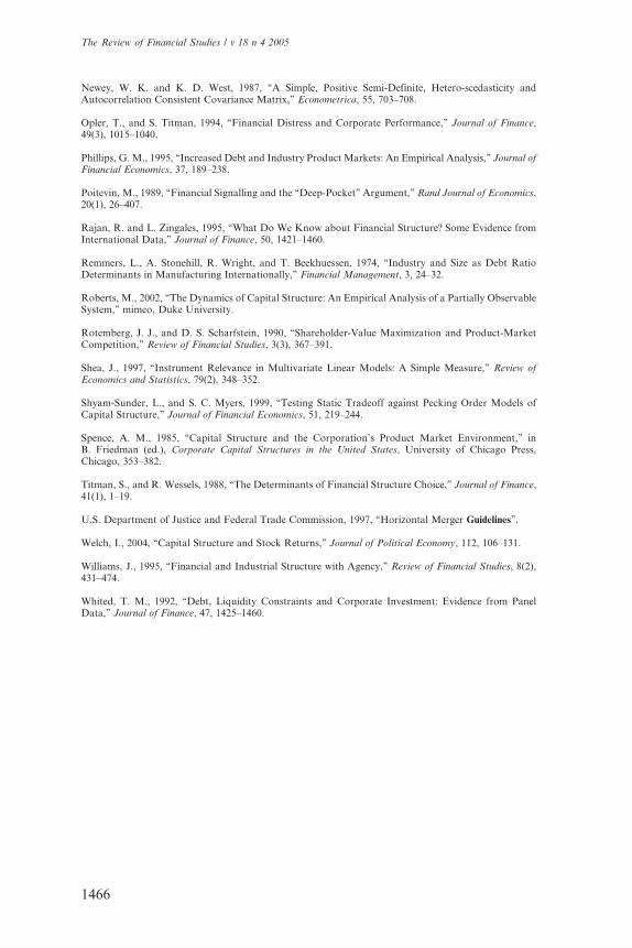
Newey, W. K. and K. D. West, 1987, ‘‘A Simple, Positive Semi-Definite, Hetero-scedasticity andAutocorrelation Consistent Covariance Matrix,’’ Econometrica, 55, 703–708.
Opler, T., and S. Titman, 1994, ‘‘Financial Distress and Corporate Performance,’’ Journal of Finance,49(3), 1015–1040.
Phillips, G. M., 1995, ‘‘Increased Debt and Industry Product Markets: An Empirical Analysis,’’ Journal ofFinancial Economics, 37, 189–238.
Poitevin, M., 1989, ‘‘Financial Signalling and the ‘‘Deep-Pocket’’ Argument,’’ Rand Journal of Economics,20(1), 26–407.
Rajan, R. and L. Zingales, 1995, ‘‘What Do We Know about Financial Structure? Some Evidence fromInternational Data,’’ Journal of Finance, 50, 1421–1460.
Remmers, L., A. Stonehill, R. Wright, and T. Beekhuessen, 1974, ‘‘Industry and Size as Debt RatioDeterminants in Manufacturing Internationally,’’ Financial Management, 3, 24–32.
Roberts, M., 2002, ‘‘The Dynamics of Capital Structure: An Empirical Analysis of a Partially ObservableSystem,’’ mimeo, Duke University.
Rotemberg, J. J., and D. S. Scharfstein, 1990, ‘‘Shareholder-Value Maximization and Product-MarketCompetition,’’ Review of Financial Studies, 3(3), 367–391.
Shea, J., 1997, ‘‘Instrument Relevance in Multivariate Linear Models: A Simple Measure,’’ Review ofEconomics and Statistics, 79(2), 348–352.
Shyam-Sunder, L., and S. C. Myers, 1999, ‘‘Testing Static Tradeoff against Pecking Order Models ofCapital Structure,’’ Journal of Financial Economics, 51, 219–244.
Spence, A. M., 1985, ‘‘Capital Structure and the Corporation’s Product Market Environment,’’ inB. Friedman (ed.), Corporate Capital Structures in the United States, University of Chicago Press,Chicago, 353–382.
Titman, S., and R. Wessels, 1988, ‘‘The Determinants of Financial Structure Choice,’’ Journal of Finance,41(1), 1–19.
U.S. Department of Justice and Federal Trade Commission, 1997, ‘‘Horizontal Merger Guidelines’’.
Welch, I., 2004, ‘‘Capital Structure and Stock Returns,’’ Journal of Political Economy, 112, 106–131.
Williams, J., 1995, ‘‘Financial and Industrial Structure with Agency,’’ Review of Financial Studies, 8(2),431–474.
Whited, T. M., 1992, ‘‘Debt, Liquidity Constraints and Corporate Investment: Evidence from PanelData,’’ Journal of Finance, 47, 1425–1460.
The Review of Financial Studies / v 18 n 4 2005
1466