
MONETARY POLICY INSTRUMENTS IN THE REPUBLIC OF CROATIA Monetary policy.

90NBB Economic Review ¡ September 2021 ¡ How do monetary policy instruments affect economy ?
How do standard and new monetary policy instruments affect the economy of the euro area and Belgium ? Estimation challenges and results
M. Deroose *
Introduction
How does monetary policy affect the economy ? This is a central question in macroeconomics, which a vast range of literature has explored and continues to do so. With respect to the impact of changes in short-term policy interest rates – being the standard monetary policy instrument – a relative consensus has been established, which entails in brief that an unexpected rise in the policy rate results in a hump-shaped temporary decline in economic activity, while the price level decreases persistently. The many studies conducted and the long experience with the policy rate instrument have given central banks a reasonably good understanding of how interest rate changes are transmitted through the economy.
However, over the past decade, policy rates in many advanced economies, including the euro area, have been constrained by the lower bound and central banks have had to expand their toolbox – deploying new measures such as forward guidance and large-scale asset purchases. Instead of seeking to influence short rates, these new measures are geared towards lowering longer rates 1. By doing so, they ensure that central banks are still able to stimulate the economy and raise inflation towards the objective even when they can no longer cut policy rates. Given that these instruments were very experimental when they were first implemented (i.e. they were labelled “non-standard” or “unconventional”), little was known about their transmission. Identifying and estimating the impact of these new monetary policy instruments has also brought novel challenges, which have (in part) been overcome by innovations in modelling.
Consequently, we now have an indication of how new monetary policy instruments affect the economy, with studies to date generally concluding that they have contributed to the functioning of financial markets and were successful in providing additional macroeconomic stimulus 2. In light of its strategy review launched in January 2020, the European Central Bank (ECB) also assessed the appropriateness of its new instruments, with the outcome being that policy rates remain the primary monetary policy instrument but that the new measures are also “an integral part of the toolbox, to be used as appropriate” 3.
* The author would like to thank Jef Boeckx, Geert Langenus, Raf Wouters and Joris Wauters for useful comments and suggestions.1 Forward guidance (i.e. central bank communication on the future stance of monetary policy), for instance, primarily works through
impacting interest-rate expectations whereby indications that policy will remain accommodative for a period of time reduce longer rates. In contrast, central bank asset purchases work primarily through compressing term and risk premia in longer rates.
2 See, for instance, BIS (2019) for a general overview of the effectiveness of non-standard monetary policy tools and Rostagno et al. (2021) for euro area evidence.
3 See the ECB press conference on the outcome of the strategy review by Christine Lagarde and Luis de Guindos on 8 July 2021.

91NBB Economic Review ¡ September 2021 ¡ How do monetary policy instruments affect economy ?
Given that non-standard monetary policy measures are (likely) to become part of the standard monetary policy toolkit, this article aims to provide an overview of the issues involved when estimating their effectiveness and it gives an illustration of their propagation in a vector autoregression (VAR) model using euro area and Belgian data. More specifically, the first section discusses the many challenges that come with documenting the causal effect of monetary policy : it explains why observed changes in policy rates do not automatically represent monetary policy shocks, what identification problem needs to be overcome in a VAR and what kind of additional complications new measures bring. The second section highlights the research efforts that have been made to deepen our knowledge about the effects of monetary policy. It briefly discusses several methods that have been developed to tackle the identification problem in a VAR, paying particular attention to recent innovations. The last section singles out one identification method to empirically illustrate the dynamic impact of the ECB’s standard and new monetary policy measures (while controlling for central bank information shocks). The analysis considers standard monetary policy to work via changes in the short rate and new monetary policy measures via changes in the long rate. The results focus in first instance on the transmission in the euro area economy, indicating that an unexpected tightening in both the standard and new monetary policy instruments lowers euro area GDP and prices (to quite a similar degree). The impact of both shocks on the Belgian economy is also briefly assessed ; it appears broadly in line with that on the euro area as a whole.
1. The many challenges of documenting the causal effect of monetary policy
This section starts with a general explainer on endogenous versus exogenous changes in monetary policy and the challenge of disentangling the two. It then turns to more technical issues, briefly sketching the identification problem in a VAR and highlighting some additional challenges associated with the identification and estimation of non-standard monetary policy shocks.
1.1 Endogenous versus exogenous changes in monetary policy
Most movements in monetary policy instruments are endogenous : they reflect the systematic reaction of monetary policy to economic circumstances. Central banks typically pursue their price stability objective by conducting a consistent and predictable monetary policy, as this helps private agents to correctly form expectations and contributes to more stable inflation and output. Therefore, the systematic reaction, that is the expected policy behaviour, affects the impact and transmission of all shocks that hit the economy. This systematic behaviour can be captured by a simple policy rule or reaction function. According to the Taylor rule (Taylor, 1993), for instance, the central bank sets the short-term policy rate in relation to the equilibrium rate 1, and in response to observed changes in inflation from its target and in output from its potential level 2. Note that this notion of the reaction function can be generalised to other monetary policy instruments such as forward guidance and central bank asset purchases.
Monetary policy can also deviate from this systematic rule-based behaviour and surprise economic agents. This reflects the non-systematic or exogenous component of monetary policy (i.e. a “shock”), as it is not related to movements in other variables. Monetary policy shocks do not account for an important share of the fluctuations in the policy instrument, nor do they induce large macroeconomic fluctuations 3. Their identification is nonetheless of interest as they can inform us about the transmission of monetary policy actions in isolation,
1 The equilibrium rate (or “natural” rate) can be defined as the interest rate consistent with output equaling potential and inflation being stable.2 Potential output reflects the (hypothetical) level of economic activity that can be obtained through the normal use of available production
factors, i.e. without generating inflationary pressures.3 For instance, Boeckx et al. (2018) – using the NBB’s DSGE model – estimate that standard monetary policy shocks would explain only 7 %
of the variations in the short-term interest rate during the period from 1995 to 2012. In contrast, the endogenous response of monetary policy to shocks hitting in the economy, via the estimated Taylor rule, would make a major contribution.

92NBB Economic Review ¡ September 2021 ¡ How do monetary policy instruments affect economy ?
i.e. they give a clean view on the causal macroeconomic effects of monetary policy. Therefore, a lot of the literature has tried to identify monetary policy shocks.
Distinguishing the systematic part from the surprises in the dynamics of the policy instruments is challenging. Structural models are needed to separate exogenous from endogenous changes in monetary policy and to analyse their propagation (via impulse response functions). In this respect, atheoretical vector autoregression (VAR) models (which are the focus of this article) and, more recently, dynamic stochastic general equilibrium (DSGE) models are both widely used. Another complication is that because monetary policy has been conducted in a systematic way in recent decades, true monetary policy shocks might be rare, and thus difficult to extract. In this respect, Ramey (2016, p. 46) soberingly notes that “It is likely that what we now identify as monetary policy shocks are mostly the effects of superior information on the part of the central bank, foresight by agents and noise. While this is bad news for econometric identification, it is good news for economic policy”.
1.2 The identification problem in a VAR
A VAR model imposes very little theoretical structure on the data 1. Under this methodology, structural shocks – which represent the exogenous disturbances of interest (such as a monetary policy shock) but which are unfortunately not directly observable – are recovered following a two-step approach, which the following sets out concisely 2.
First, a reduced-form VAR is estimated :
where
4
1.2. The identification problem in a VAR
A VAR model imposes very little theoretical structure on the data1. Under this methodology, structural shocks – which represent the exogenous disturbances of interest (such as a monetary policy shock) but which are unfortunately not directly observable – are recovered following a two-step approach, which the following sets out concisely2.
First, a reduced-form VAR is estimated:
𝑌𝑌𝑡𝑡 = 𝐴𝐴0 + 𝐴𝐴1𝑌𝑌𝑡𝑡−1+. . . + 𝐴𝐴𝑝𝑝𝑌𝑌𝑡𝑡−𝑝𝑝 + 𝑒𝑒𝑡𝑡,
where 𝑌𝑌𝑡𝑡 is a vector of endogenous variables (consisting, for example, of output, inflation and the policy rate) and 𝑒𝑒𝑡𝑡 are serially uncorrelated but mutually correlated residuals. The reduced-form VAR relates each variable in the vector 𝑌𝑌𝑡𝑡 to past values of itself and the other variables in 𝑌𝑌𝑡𝑡. Through regressing 𝑌𝑌𝑖𝑖𝑡𝑡 onto p-lagged values of 𝑌𝑌𝑡𝑡, the coefficient matrices 𝐴𝐴0, … , 𝐴𝐴𝑝𝑝 and the residuals 𝑒𝑒𝑡𝑡 are obtained. The accuracy of the analysis depends, inter alia, on how accurately the selected variables and estimated coefficients describe the systematic response of monetary policy to the economy, i.e. to what extent it captures the “true” monetary policy rule.
The next challenge is then to recover the unobserved structural shocks 𝜀𝜀𝑡𝑡 of interest, including the monetary policy shock. The VAR assumes that the estimated residuals 𝑒𝑒𝑡𝑡 are a linear combination of the structural independent shocks 𝜀𝜀𝑡𝑡:
𝑒𝑒𝑡𝑡 = 𝐵𝐵0𝜀𝜀𝑡𝑡,
– where the impact matrix 𝐵𝐵0 defines the statistical residuals as linearcombinations of the structural shocks. The structural shocks can then be identified by applying identification restrictions on 𝐵𝐵0. The task of identifying the structural shock of interest thus comes down to finding the linear combination of residuals that makes up the structural shock. It should be noted that the outcomes of the VAR analysis depend crucially on the additionally imposed assumptions. For the shocks identified through restrictions on 𝐵𝐵0 to accurately capture the true monetary policy shock, the restrictions on 𝐵𝐵0 must successfully isolate the monetary policy shock from any other shocks that impact the macroeconomic variables, including the policy rate. In other words, the structural shocks must be uncorrelated, making them exogenous. In many cases, the researcher may only be interested in the effect of a single shock, for example, a monetary policy shock. In general, the other shocks need not be identified to obtain the structural impulse response to that shock. A single shock identification thus requires less restrictions to be imposed on 𝐵𝐵0 than the full shock identification.
Based on the reduced-form coefficients and the structural shocks, one can then trace the dynamic response of each variable to the identified structural shock.
1.3. Complications when identifying non-standard monetary policy shocks
Like with traditional monetary policy shocks, the endogeneity issue implied by the systematic behaviour of monetary policy complicates the identification of non-standard monetary policy shocks. But identifying and estimating the effect of new measures also brings new challenges. A specific issue that pops up, for example, is how to identify the impact of individual new measures as often different measures were announced at the same time. In addition, new measures (regarding central bank asset purchases, for example,) were often pre-announced, making it difficult to precisely identify the shocks. Focusing specifically on the long-term interest rate – which tends to be the more relevant variable that is directly targeted by new monetary policy instruments like forward guidance and asset purchases –, the identification of exogenous changes also proves to be more challenging than when considering the short-term policy rate, as long-term rates are affected by many more variables beyond monetary policy decisions, such as private sector expectations about the future state of the
1 In contrast, a DSGE model imposes a fully specified structure on the data. This structure consists of a set of equations, derived from theory, assembled in a consistent way so as
to describe the relevant macroeconomic interactions of an economy. Shocks, which are the source of macroeconomic fluctuations in the model, are identified by this theoretical structure (they are called “structural” shocks). When the model is brought to the data, these shocks and the associated impulse responses of macro variables are estimated. An estimated monetary policy rule equation is used to distinguish the systematic component of monetary policy from the unexpected monetary policy shock.
2 For a more comprehensive overview of the identification problem, associated complications and pitfalls, see, for example, Ramey (2016), Stock and Watson (2016) and Rossi (2019).
is a vector of endogenous variables (consisting, for example, of output, inflation and the policy rate) and
4
1.2. The identification problem in a VAR
A VAR model imposes very little theoretical structure on the data1. Under this methodology, structural shocks – which represent the exogenous disturbances of interest (such as a monetary policy shock) but which are unfortunately not directly observable – are recovered following a two-step approach, which the following sets out concisely2.
First, a reduced-form VAR is estimated:
𝑌𝑌𝑡𝑡 = 𝐴𝐴0 + 𝐴𝐴1𝑌𝑌𝑡𝑡−1+. . . + 𝐴𝐴𝑝𝑝𝑌𝑌𝑡𝑡−𝑝𝑝 + 𝑒𝑒𝑡𝑡,
where 𝑌𝑌𝑡𝑡 is a vector of endogenous variables (consisting, for example, of output, inflation and the policy rate) and 𝑒𝑒𝑡𝑡 are serially uncorrelated but mutually correlated residuals. The reduced-form VAR relates each variable in the vector 𝑌𝑌𝑡𝑡 to past values of itself and the other variables in 𝑌𝑌𝑡𝑡. Through regressing 𝑌𝑌𝑖𝑖𝑡𝑡 onto p-lagged values of 𝑌𝑌𝑡𝑡, the coefficient matrices 𝐴𝐴0, … , 𝐴𝐴𝑝𝑝 and the residuals 𝑒𝑒𝑡𝑡 are obtained. The accuracy of the analysis depends, inter alia, on how accurately the selected variables and estimated coefficients describe the systematic response of monetary policy to the economy, i.e. to what extent it captures the “true” monetary policy rule.
The next challenge is then to recover the unobserved structural shocks 𝜀𝜀𝑡𝑡 of interest, including the monetary policy shock. The VAR assumes that the estimated residuals 𝑒𝑒𝑡𝑡 are a linear combination of the structural independent shocks 𝜀𝜀𝑡𝑡:
𝑒𝑒𝑡𝑡 = 𝐵𝐵0𝜀𝜀𝑡𝑡,
– where the impact matrix 𝐵𝐵0 defines the statistical residuals as linearcombinations of the structural shocks. The structural shocks can then be identified by applying identification restrictions on 𝐵𝐵0. The task of identifying the structural shock of interest thus comes down to finding the linear combination of residuals that makes up the structural shock. It should be noted that the outcomes of the VAR analysis depend crucially on the additionally imposed assumptions. For the shocks identified through restrictions on 𝐵𝐵0 to accurately capture the true monetary policy shock, the restrictions on 𝐵𝐵0 must successfully isolate the monetary policy shock from any other shocks that impact the macroeconomic variables, including the policy rate. In other words, the structural shocks must be uncorrelated, making them exogenous. In many cases, the researcher may only be interested in the effect of a single shock, for example, a monetary policy shock. In general, the other shocks need not be identified to obtain the structural impulse response to that shock. A single shock identification thus requires less restrictions to be imposed on 𝐵𝐵0 than the full shock identification.
Based on the reduced-form coefficients and the structural shocks, one can then trace the dynamic response of each variable to the identified structural shock.
1.3. Complications when identifying non-standard monetary policy shocks
Like with traditional monetary policy shocks, the endogeneity issue implied by the systematic behaviour of monetary policy complicates the identification of non-standard monetary policy shocks. But identifying and estimating the effect of new measures also brings new challenges. A specific issue that pops up, for example, is how to identify the impact of individual new measures as often different measures were announced at the same time. In addition, new measures (regarding central bank asset purchases, for example,) were often pre-announced, making it difficult to precisely identify the shocks. Focusing specifically on the long-term interest rate – which tends to be the more relevant variable that is directly targeted by new monetary policy instruments like forward guidance and asset purchases –, the identification of exogenous changes also proves to be more challenging than when considering the short-term policy rate, as long-term rates are affected by many more variables beyond monetary policy decisions, such as private sector expectations about the future state of the
1 In contrast, a DSGE model imposes a fully specified structure on the data. This structure consists of a set of equations, derived from theory, assembled in a consistent way so as
to describe the relevant macroeconomic interactions of an economy. Shocks, which are the source of macroeconomic fluctuations in the model, are identified by this theoretical structure (they are called “structural” shocks). When the model is brought to the data, these shocks and the associated impulse responses of macro variables are estimated. An estimated monetary policy rule equation is used to distinguish the systematic component of monetary policy from the unexpected monetary policy shock.
2 For a more comprehensive overview of the identification problem, associated complications and pitfalls, see, for example, Ramey (2016), Stock and Watson (2016) and Rossi (2019).
are serially uncorrelated but mutually correlated residuals. The reduced-form VAR relates each variable in the vector
4
1.2. The identification problem in a VAR
A VAR model imposes very little theoretical structure on the data1. Under this methodology, structural shocks – which represent the exogenous disturbances of interest (such as a monetary policy shock) but which are unfortunately not directly observable – are recovered following a two-step approach, which the following sets out concisely2.
First, a reduced-form VAR is estimated:
𝑌𝑌𝑡𝑡 = 𝐴𝐴0 + 𝐴𝐴1𝑌𝑌𝑡𝑡−1+. . . + 𝐴𝐴𝑝𝑝𝑌𝑌𝑡𝑡−𝑝𝑝 + 𝑒𝑒𝑡𝑡,
where 𝑌𝑌𝑡𝑡 is a vector of endogenous variables (consisting, for example, of output, inflation and the policy rate) and 𝑒𝑒𝑡𝑡 are serially uncorrelated but mutually correlated residuals. The reduced-form VAR relates each variable in the vector 𝑌𝑌𝑡𝑡 to past values of itself and the other variables in 𝑌𝑌𝑡𝑡. Through regressing 𝑌𝑌𝑖𝑖𝑡𝑡 onto p-lagged values of 𝑌𝑌𝑡𝑡, the coefficient matrices 𝐴𝐴0, … , 𝐴𝐴𝑝𝑝 and the residuals 𝑒𝑒𝑡𝑡 are obtained. The accuracy of the analysis depends, inter alia, on how accurately the selected variables and estimated coefficients describe the systematic response of monetary policy to the economy, i.e. to what extent it captures the “true” monetary policy rule.
The next challenge is then to recover the unobserved structural shocks 𝜀𝜀𝑡𝑡 of interest, including the monetary policy shock. The VAR assumes that the estimated residuals 𝑒𝑒𝑡𝑡 are a linear combination of the structural independent shocks 𝜀𝜀𝑡𝑡:
𝑒𝑒𝑡𝑡 = 𝐵𝐵0𝜀𝜀𝑡𝑡,
– where the impact matrix 𝐵𝐵0 defines the statistical residuals as linearcombinations of the structural shocks. The structural shocks can then be identified by applying identification restrictions on 𝐵𝐵0. The task of identifying the structural shock of interest thus comes down to finding the linear combination of residuals that makes up the structural shock. It should be noted that the outcomes of the VAR analysis depend crucially on the additionally imposed assumptions. For the shocks identified through restrictions on 𝐵𝐵0 to accurately capture the true monetary policy shock, the restrictions on 𝐵𝐵0 must successfully isolate the monetary policy shock from any other shocks that impact the macroeconomic variables, including the policy rate. In other words, the structural shocks must be uncorrelated, making them exogenous. In many cases, the researcher may only be interested in the effect of a single shock, for example, a monetary policy shock. In general, the other shocks need not be identified to obtain the structural impulse response to that shock. A single shock identification thus requires less restrictions to be imposed on 𝐵𝐵0 than the full shock identification.
Based on the reduced-form coefficients and the structural shocks, one can then trace the dynamic response of each variable to the identified structural shock.
1.3. Complications when identifying non-standard monetary policy shocks
Like with traditional monetary policy shocks, the endogeneity issue implied by the systematic behaviour of monetary policy complicates the identification of non-standard monetary policy shocks. But identifying and estimating the effect of new measures also brings new challenges. A specific issue that pops up, for example, is how to identify the impact of individual new measures as often different measures were announced at the same time. In addition, new measures (regarding central bank asset purchases, for example,) were often pre-announced, making it difficult to precisely identify the shocks. Focusing specifically on the long-term interest rate – which tends to be the more relevant variable that is directly targeted by new monetary policy instruments like forward guidance and asset purchases –, the identification of exogenous changes also proves to be more challenging than when considering the short-term policy rate, as long-term rates are affected by many more variables beyond monetary policy decisions, such as private sector expectations about the future state of the
1 In contrast, a DSGE model imposes a fully specified structure on the data. This structure consists of a set of equations, derived from theory, assembled in a consistent way so as
to describe the relevant macroeconomic interactions of an economy. Shocks, which are the source of macroeconomic fluctuations in the model, are identified by this theoretical structure (they are called “structural” shocks). When the model is brought to the data, these shocks and the associated impulse responses of macro variables are estimated. An estimated monetary policy rule equation is used to distinguish the systematic component of monetary policy from the unexpected monetary policy shock.
2 For a more comprehensive overview of the identification problem, associated complications and pitfalls, see, for example, Ramey (2016), Stock and Watson (2016) and Rossi (2019).
to past values of itself and the other variables in
4
1.2. The identification problem in a VAR
A VAR model imposes very little theoretical structure on the data1. Under this methodology, structural shocks – which represent the exogenous disturbances of interest (such as a monetary policy shock) but which are unfortunately not directly observable – are recovered following a two-step approach, which the following sets out concisely2.
First, a reduced-form VAR is estimated:
𝑌𝑌𝑡𝑡 = 𝐴𝐴0 + 𝐴𝐴1𝑌𝑌𝑡𝑡−1+. . . + 𝐴𝐴𝑝𝑝𝑌𝑌𝑡𝑡−𝑝𝑝 + 𝑒𝑒𝑡𝑡,
where 𝑌𝑌𝑡𝑡 is a vector of endogenous variables (consisting, for example, of output, inflation and the policy rate) and 𝑒𝑒𝑡𝑡 are serially uncorrelated but mutually correlated residuals. The reduced-form VAR relates each variable in the vector 𝑌𝑌𝑡𝑡 to past values of itself and the other variables in 𝑌𝑌𝑡𝑡. Through regressing 𝑌𝑌𝑖𝑖𝑡𝑡 onto p-lagged values of 𝑌𝑌𝑡𝑡, the coefficient matrices 𝐴𝐴0, … , 𝐴𝐴𝑝𝑝 and the residuals 𝑒𝑒𝑡𝑡 are obtained. The accuracy of the analysis depends, inter alia, on how accurately the selected variables and estimated coefficients describe the systematic response of monetary policy to the economy, i.e. to what extent it captures the “true” monetary policy rule.
The next challenge is then to recover the unobserved structural shocks 𝜀𝜀𝑡𝑡 of interest, including the monetary policy shock. The VAR assumes that the estimated residuals 𝑒𝑒𝑡𝑡 are a linear combination of the structural independent shocks 𝜀𝜀𝑡𝑡:
𝑒𝑒𝑡𝑡 = 𝐵𝐵0𝜀𝜀𝑡𝑡,
– where the impact matrix 𝐵𝐵0 defines the statistical residuals as linearcombinations of the structural shocks. The structural shocks can then be identified by applying identification restrictions on 𝐵𝐵0. The task of identifying the structural shock of interest thus comes down to finding the linear combination of residuals that makes up the structural shock. It should be noted that the outcomes of the VAR analysis depend crucially on the additionally imposed assumptions. For the shocks identified through restrictions on 𝐵𝐵0 to accurately capture the true monetary policy shock, the restrictions on 𝐵𝐵0 must successfully isolate the monetary policy shock from any other shocks that impact the macroeconomic variables, including the policy rate. In other words, the structural shocks must be uncorrelated, making them exogenous. In many cases, the researcher may only be interested in the effect of a single shock, for example, a monetary policy shock. In general, the other shocks need not be identified to obtain the structural impulse response to that shock. A single shock identification thus requires less restrictions to be imposed on 𝐵𝐵0 than the full shock identification.
Based on the reduced-form coefficients and the structural shocks, one can then trace the dynamic response of each variable to the identified structural shock.
1.3. Complications when identifying non-standard monetary policy shocks
Like with traditional monetary policy shocks, the endogeneity issue implied by the systematic behaviour of monetary policy complicates the identification of non-standard monetary policy shocks. But identifying and estimating the effect of new measures also brings new challenges. A specific issue that pops up, for example, is how to identify the impact of individual new measures as often different measures were announced at the same time. In addition, new measures (regarding central bank asset purchases, for example,) were often pre-announced, making it difficult to precisely identify the shocks. Focusing specifically on the long-term interest rate – which tends to be the more relevant variable that is directly targeted by new monetary policy instruments like forward guidance and asset purchases –, the identification of exogenous changes also proves to be more challenging than when considering the short-term policy rate, as long-term rates are affected by many more variables beyond monetary policy decisions, such as private sector expectations about the future state of the
1 In contrast, a DSGE model imposes a fully specified structure on the data. This structure consists of a set of equations, derived from theory, assembled in a consistent way so as
to describe the relevant macroeconomic interactions of an economy. Shocks, which are the source of macroeconomic fluctuations in the model, are identified by this theoretical structure (they are called “structural” shocks). When the model is brought to the data, these shocks and the associated impulse responses of macro variables are estimated. An estimated monetary policy rule equation is used to distinguish the systematic component of monetary policy from the unexpected monetary policy shock.
2 For a more comprehensive overview of the identification problem, associated complications and pitfalls, see, for example, Ramey (2016), Stock and Watson (2016) and Rossi (2019).
. Through regressing
4
1.2. The identification problem in a VAR
A VAR model imposes very little theoretical structure on the data1. Under this methodology, structural shocks – which represent the exogenous disturbances of interest (such as a monetary policy shock) but which are unfortunately not directly observable – are recovered following a two-step approach, which the following sets out concisely2.
First, a reduced-form VAR is estimated:
𝑌𝑌𝑡𝑡 = 𝐴𝐴0 + 𝐴𝐴1𝑌𝑌𝑡𝑡−1+. . . + 𝐴𝐴𝑝𝑝𝑌𝑌𝑡𝑡−𝑝𝑝 + 𝑒𝑒𝑡𝑡,
where 𝑌𝑌𝑡𝑡 is a vector of endogenous variables (consisting, for example, of output, inflation and the policy rate) and 𝑒𝑒𝑡𝑡 are serially uncorrelated but mutually correlated residuals. The reduced-form VAR relates each variable in the vector 𝑌𝑌𝑡𝑡 to past values of itself and the other variables in 𝑌𝑌𝑡𝑡. Through regressing 𝑌𝑌𝑖𝑖𝑡𝑡 onto p-lagged values of 𝑌𝑌𝑡𝑡, the coefficient matrices 𝐴𝐴0, … , 𝐴𝐴𝑝𝑝 and the residuals 𝑒𝑒𝑡𝑡 are obtained. The accuracy of the analysis depends, inter alia, on how accurately the selected variables and estimated coefficients describe the systematic response of monetary policy to the economy, i.e. to what extent it captures the “true” monetary policy rule.
The next challenge is then to recover the unobserved structural shocks 𝜀𝜀𝑡𝑡 of interest, including the monetary policy shock. The VAR assumes that the estimated residuals 𝑒𝑒𝑡𝑡 are a linear combination of the structural independent shocks 𝜀𝜀𝑡𝑡:
𝑒𝑒𝑡𝑡 = 𝐵𝐵0𝜀𝜀𝑡𝑡,
– where the impact matrix 𝐵𝐵0 defines the statistical residuals as linearcombinations of the structural shocks. The structural shocks can then be identified by applying identification restrictions on 𝐵𝐵0. The task of identifying the structural shock of interest thus comes down to finding the linear combination of residuals that makes up the structural shock. It should be noted that the outcomes of the VAR analysis depend crucially on the additionally imposed assumptions. For the shocks identified through restrictions on 𝐵𝐵0 to accurately capture the true monetary policy shock, the restrictions on 𝐵𝐵0 must successfully isolate the monetary policy shock from any other shocks that impact the macroeconomic variables, including the policy rate. In other words, the structural shocks must be uncorrelated, making them exogenous. In many cases, the researcher may only be interested in the effect of a single shock, for example, a monetary policy shock. In general, the other shocks need not be identified to obtain the structural impulse response to that shock. A single shock identification thus requires less restrictions to be imposed on 𝐵𝐵0 than the full shock identification.
Based on the reduced-form coefficients and the structural shocks, one can then trace the dynamic response of each variable to the identified structural shock.
1.3. Complications when identifying non-standard monetary policy shocks
Like with traditional monetary policy shocks, the endogeneity issue implied by the systematic behaviour of monetary policy complicates the identification of non-standard monetary policy shocks. But identifying and estimating the effect of new measures also brings new challenges. A specific issue that pops up, for example, is how to identify the impact of individual new measures as often different measures were announced at the same time. In addition, new measures (regarding central bank asset purchases, for example,) were often pre-announced, making it difficult to precisely identify the shocks. Focusing specifically on the long-term interest rate – which tends to be the more relevant variable that is directly targeted by new monetary policy instruments like forward guidance and asset purchases –, the identification of exogenous changes also proves to be more challenging than when considering the short-term policy rate, as long-term rates are affected by many more variables beyond monetary policy decisions, such as private sector expectations about the future state of the
1 In contrast, a DSGE model imposes a fully specified structure on the data. This structure consists of a set of equations, derived from theory, assembled in a consistent way so as
to describe the relevant macroeconomic interactions of an economy. Shocks, which are the source of macroeconomic fluctuations in the model, are identified by this theoretical structure (they are called “structural” shocks). When the model is brought to the data, these shocks and the associated impulse responses of macro variables are estimated. An estimated monetary policy rule equation is used to distinguish the systematic component of monetary policy from the unexpected monetary policy shock.
2 For a more comprehensive overview of the identification problem, associated complications and pitfalls, see, for example, Ramey (2016), Stock and Watson (2016) and Rossi (2019).
onto p-lagged values of
4
1.2. The identification problem in a VAR
A VAR model imposes very little theoretical structure on the data1. Under this methodology, structural shocks – which represent the exogenous disturbances of interest (such as a monetary policy shock) but which are unfortunately not directly observable – are recovered following a two-step approach, which the following sets out concisely2.
First, a reduced-form VAR is estimated:
𝑌𝑌𝑡𝑡 = 𝐴𝐴0 + 𝐴𝐴1𝑌𝑌𝑡𝑡−1+. . . + 𝐴𝐴𝑝𝑝𝑌𝑌𝑡𝑡−𝑝𝑝 + 𝑒𝑒𝑡𝑡,
where 𝑌𝑌𝑡𝑡 is a vector of endogenous variables (consisting, for example, of output, inflation and the policy rate) and 𝑒𝑒𝑡𝑡 are serially uncorrelated but mutually correlated residuals. The reduced-form VAR relates each variable in the vector 𝑌𝑌𝑡𝑡 to past values of itself and the other variables in 𝑌𝑌𝑡𝑡. Through regressing 𝑌𝑌𝑖𝑖𝑡𝑡 onto p-lagged values of 𝑌𝑌𝑡𝑡, the coefficient matrices 𝐴𝐴0, … , 𝐴𝐴𝑝𝑝 and the residuals 𝑒𝑒𝑡𝑡 are obtained. The accuracy of the analysis depends, inter alia, on how accurately the selected variables and estimated coefficients describe the systematic response of monetary policy to the economy, i.e. to what extent it captures the “true” monetary policy rule.
The next challenge is then to recover the unobserved structural shocks 𝜀𝜀𝑡𝑡 of interest, including the monetary policy shock. The VAR assumes that the estimated residuals 𝑒𝑒𝑡𝑡 are a linear combination of the structural independent shocks 𝜀𝜀𝑡𝑡:
𝑒𝑒𝑡𝑡 = 𝐵𝐵0𝜀𝜀𝑡𝑡,
– where the impact matrix 𝐵𝐵0 defines the statistical residuals as linearcombinations of the structural shocks. The structural shocks can then be identified by applying identification restrictions on 𝐵𝐵0. The task of identifying the structural shock of interest thus comes down to finding the linear combination of residuals that makes up the structural shock. It should be noted that the outcomes of the VAR analysis depend crucially on the additionally imposed assumptions. For the shocks identified through restrictions on 𝐵𝐵0 to accurately capture the true monetary policy shock, the restrictions on 𝐵𝐵0 must successfully isolate the monetary policy shock from any other shocks that impact the macroeconomic variables, including the policy rate. In other words, the structural shocks must be uncorrelated, making them exogenous. In many cases, the researcher may only be interested in the effect of a single shock, for example, a monetary policy shock. In general, the other shocks need not be identified to obtain the structural impulse response to that shock. A single shock identification thus requires less restrictions to be imposed on 𝐵𝐵0 than the full shock identification.
Based on the reduced-form coefficients and the structural shocks, one can then trace the dynamic response of each variable to the identified structural shock.
1.3. Complications when identifying non-standard monetary policy shocks
Like with traditional monetary policy shocks, the endogeneity issue implied by the systematic behaviour of monetary policy complicates the identification of non-standard monetary policy shocks. But identifying and estimating the effect of new measures also brings new challenges. A specific issue that pops up, for example, is how to identify the impact of individual new measures as often different measures were announced at the same time. In addition, new measures (regarding central bank asset purchases, for example,) were often pre-announced, making it difficult to precisely identify the shocks. Focusing specifically on the long-term interest rate – which tends to be the more relevant variable that is directly targeted by new monetary policy instruments like forward guidance and asset purchases –, the identification of exogenous changes also proves to be more challenging than when considering the short-term policy rate, as long-term rates are affected by many more variables beyond monetary policy decisions, such as private sector expectations about the future state of the
1 In contrast, a DSGE model imposes a fully specified structure on the data. This structure consists of a set of equations, derived from theory, assembled in a consistent way so as
to describe the relevant macroeconomic interactions of an economy. Shocks, which are the source of macroeconomic fluctuations in the model, are identified by this theoretical structure (they are called “structural” shocks). When the model is brought to the data, these shocks and the associated impulse responses of macro variables are estimated. An estimated monetary policy rule equation is used to distinguish the systematic component of monetary policy from the unexpected monetary policy shock.
2 For a more comprehensive overview of the identification problem, associated complications and pitfalls, see, for example, Ramey (2016), Stock and Watson (2016) and Rossi (2019).
, the coefficient matrices
4
1.2. The identification problem in a VAR
A VAR model imposes very little theoretical structure on the data1. Under this methodology, structural shocks – which represent the exogenous disturbances of interest (such as a monetary policy shock) but which are unfortunately not directly observable – are recovered following a two-step approach, which the following sets out concisely2.
First, a reduced-form VAR is estimated:
𝑌𝑌𝑡𝑡 = 𝐴𝐴0 + 𝐴𝐴1𝑌𝑌𝑡𝑡−1+. . . + 𝐴𝐴𝑝𝑝𝑌𝑌𝑡𝑡−𝑝𝑝 + 𝑒𝑒𝑡𝑡,
where 𝑌𝑌𝑡𝑡 is a vector of endogenous variables (consisting, for example, of output, inflation and the policy rate) and 𝑒𝑒𝑡𝑡 are serially uncorrelated but mutually correlated residuals. The reduced-form VAR relates each variable in the vector 𝑌𝑌𝑡𝑡 to past values of itself and the other variables in 𝑌𝑌𝑡𝑡. Through regressing 𝑌𝑌𝑖𝑖𝑡𝑡 onto p-lagged values of 𝑌𝑌𝑡𝑡, the coefficient matrices 𝐴𝐴0, … , 𝐴𝐴𝑝𝑝 and the residuals 𝑒𝑒𝑡𝑡 are obtained. The accuracy of the analysis depends, inter alia, on how accurately the selected variables and estimated coefficients describe the systematic response of monetary policy to the economy, i.e. to what extent it captures the “true” monetary policy rule.
The next challenge is then to recover the unobserved structural shocks 𝜀𝜀𝑡𝑡 of interest, including the monetary policy shock. The VAR assumes that the estimated residuals 𝑒𝑒𝑡𝑡 are a linear combination of the structural independent shocks 𝜀𝜀𝑡𝑡:
𝑒𝑒𝑡𝑡 = 𝐵𝐵0𝜀𝜀𝑡𝑡,
– where the impact matrix 𝐵𝐵0 defines the statistical residuals as linearcombinations of the structural shocks. The structural shocks can then be identified by applying identification restrictions on 𝐵𝐵0. The task of identifying the structural shock of interest thus comes down to finding the linear combination of residuals that makes up the structural shock. It should be noted that the outcomes of the VAR analysis depend crucially on the additionally imposed assumptions. For the shocks identified through restrictions on 𝐵𝐵0 to accurately capture the true monetary policy shock, the restrictions on 𝐵𝐵0 must successfully isolate the monetary policy shock from any other shocks that impact the macroeconomic variables, including the policy rate. In other words, the structural shocks must be uncorrelated, making them exogenous. In many cases, the researcher may only be interested in the effect of a single shock, for example, a monetary policy shock. In general, the other shocks need not be identified to obtain the structural impulse response to that shock. A single shock identification thus requires less restrictions to be imposed on 𝐵𝐵0 than the full shock identification.
Based on the reduced-form coefficients and the structural shocks, one can then trace the dynamic response of each variable to the identified structural shock.
1.3. Complications when identifying non-standard monetary policy shocks
Like with traditional monetary policy shocks, the endogeneity issue implied by the systematic behaviour of monetary policy complicates the identification of non-standard monetary policy shocks. But identifying and estimating the effect of new measures also brings new challenges. A specific issue that pops up, for example, is how to identify the impact of individual new measures as often different measures were announced at the same time. In addition, new measures (regarding central bank asset purchases, for example,) were often pre-announced, making it difficult to precisely identify the shocks. Focusing specifically on the long-term interest rate – which tends to be the more relevant variable that is directly targeted by new monetary policy instruments like forward guidance and asset purchases –, the identification of exogenous changes also proves to be more challenging than when considering the short-term policy rate, as long-term rates are affected by many more variables beyond monetary policy decisions, such as private sector expectations about the future state of the
1 In contrast, a DSGE model imposes a fully specified structure on the data. This structure consists of a set of equations, derived from theory, assembled in a consistent way so as
to describe the relevant macroeconomic interactions of an economy. Shocks, which are the source of macroeconomic fluctuations in the model, are identified by this theoretical structure (they are called “structural” shocks). When the model is brought to the data, these shocks and the associated impulse responses of macro variables are estimated. An estimated monetary policy rule equation is used to distinguish the systematic component of monetary policy from the unexpected monetary policy shock.
2 For a more comprehensive overview of the identification problem, associated complications and pitfalls, see, for example, Ramey (2016), Stock and Watson (2016) and Rossi (2019).
and the residuals
4
1.2. The identification problem in a VAR
A VAR model imposes very little theoretical structure on the data1. Under this methodology, structural shocks – which represent the exogenous disturbances of interest (such as a monetary policy shock) but which are unfortunately not directly observable – are recovered following a two-step approach, which the following sets out concisely2.
First, a reduced-form VAR is estimated:
𝑌𝑌𝑡𝑡 = 𝐴𝐴0 + 𝐴𝐴1𝑌𝑌𝑡𝑡−1+. . . + 𝐴𝐴𝑝𝑝𝑌𝑌𝑡𝑡−𝑝𝑝 + 𝑒𝑒𝑡𝑡,
where 𝑌𝑌𝑡𝑡 is a vector of endogenous variables (consisting, for example, of output, inflation and the policy rate) and 𝑒𝑒𝑡𝑡 are serially uncorrelated but mutually correlated residuals. The reduced-form VAR relates each variable in the vector 𝑌𝑌𝑡𝑡 to past values of itself and the other variables in 𝑌𝑌𝑡𝑡. Through regressing 𝑌𝑌𝑖𝑖𝑡𝑡 onto p-lagged values of 𝑌𝑌𝑡𝑡, the coefficient matrices 𝐴𝐴0, … , 𝐴𝐴𝑝𝑝 and the residuals 𝑒𝑒𝑡𝑡 are obtained. The accuracy of the analysis depends, inter alia, on how accurately the selected variables and estimated coefficients describe the systematic response of monetary policy to the economy, i.e. to what extent it captures the “true” monetary policy rule.
The next challenge is then to recover the unobserved structural shocks 𝜀𝜀𝑡𝑡 of interest, including the monetary policy shock. The VAR assumes that the estimated residuals 𝑒𝑒𝑡𝑡 are a linear combination of the structural independent shocks 𝜀𝜀𝑡𝑡:
𝑒𝑒𝑡𝑡 = 𝐵𝐵0𝜀𝜀𝑡𝑡,
– where the impact matrix 𝐵𝐵0 defines the statistical residuals as linearcombinations of the structural shocks. The structural shocks can then be identified by applying identification restrictions on 𝐵𝐵0. The task of identifying the structural shock of interest thus comes down to finding the linear combination of residuals that makes up the structural shock. It should be noted that the outcomes of the VAR analysis depend crucially on the additionally imposed assumptions. For the shocks identified through restrictions on 𝐵𝐵0 to accurately capture the true monetary policy shock, the restrictions on 𝐵𝐵0 must successfully isolate the monetary policy shock from any other shocks that impact the macroeconomic variables, including the policy rate. In other words, the structural shocks must be uncorrelated, making them exogenous. In many cases, the researcher may only be interested in the effect of a single shock, for example, a monetary policy shock. In general, the other shocks need not be identified to obtain the structural impulse response to that shock. A single shock identification thus requires less restrictions to be imposed on 𝐵𝐵0 than the full shock identification.
Based on the reduced-form coefficients and the structural shocks, one can then trace the dynamic response of each variable to the identified structural shock.
1.3. Complications when identifying non-standard monetary policy shocks
Like with traditional monetary policy shocks, the endogeneity issue implied by the systematic behaviour of monetary policy complicates the identification of non-standard monetary policy shocks. But identifying and estimating the effect of new measures also brings new challenges. A specific issue that pops up, for example, is how to identify the impact of individual new measures as often different measures were announced at the same time. In addition, new measures (regarding central bank asset purchases, for example,) were often pre-announced, making it difficult to precisely identify the shocks. Focusing specifically on the long-term interest rate – which tends to be the more relevant variable that is directly targeted by new monetary policy instruments like forward guidance and asset purchases –, the identification of exogenous changes also proves to be more challenging than when considering the short-term policy rate, as long-term rates are affected by many more variables beyond monetary policy decisions, such as private sector expectations about the future state of the
1 In contrast, a DSGE model imposes a fully specified structure on the data. This structure consists of a set of equations, derived from theory, assembled in a consistent way so as
to describe the relevant macroeconomic interactions of an economy. Shocks, which are the source of macroeconomic fluctuations in the model, are identified by this theoretical structure (they are called “structural” shocks). When the model is brought to the data, these shocks and the associated impulse responses of macro variables are estimated. An estimated monetary policy rule equation is used to distinguish the systematic component of monetary policy from the unexpected monetary policy shock.
2 For a more comprehensive overview of the identification problem, associated complications and pitfalls, see, for example, Ramey (2016), Stock and Watson (2016) and Rossi (2019).
are obtained. The accuracy of the analysis depends, inter alia, on how accurately the selected variables and estimated coefficients describe the systematic response of monetary policy to the economy, i.e. to what extent it captures the “true” monetary policy rule.
The next challenge is then to recover the unobserved structural shocks
4
1.2. The identification problem in a VAR
A VAR model imposes very little theoretical structure on the data1. Under this methodology, structural shocks – which represent the exogenous disturbances of interest (such as a monetary policy shock) but which are unfortunately not directly observable – are recovered following a two-step approach, which the following sets out concisely2.
First, a reduced-form VAR is estimated:
𝑌𝑌𝑡𝑡 = 𝐴𝐴0 + 𝐴𝐴1𝑌𝑌𝑡𝑡−1+. . . + 𝐴𝐴𝑝𝑝𝑌𝑌𝑡𝑡−𝑝𝑝 + 𝑒𝑒𝑡𝑡,
where 𝑌𝑌𝑡𝑡 is a vector of endogenous variables (consisting, for example, of output, inflation and the policy rate) and 𝑒𝑒𝑡𝑡 are serially uncorrelated but mutually correlated residuals. The reduced-form VAR relates each variable in the vector 𝑌𝑌𝑡𝑡 to past values of itself and the other variables in 𝑌𝑌𝑡𝑡. Through regressing 𝑌𝑌𝑖𝑖𝑡𝑡 onto p-lagged values of 𝑌𝑌𝑡𝑡, the coefficient matrices 𝐴𝐴0, … , 𝐴𝐴𝑝𝑝 and the residuals 𝑒𝑒𝑡𝑡 are obtained. The accuracy of the analysis depends, inter alia, on how accurately the selected variables and estimated coefficients describe the systematic response of monetary policy to the economy, i.e. to what extent it captures the “true” monetary policy rule.
The next challenge is then to recover the unobserved structural shocks 𝜀𝜀𝑡𝑡 of interest, including the monetary policy shock. The VAR assumes that the estimated residuals 𝑒𝑒𝑡𝑡 are a linear combination of the structural independent shocks 𝜀𝜀𝑡𝑡:
𝑒𝑒𝑡𝑡 = 𝐵𝐵0𝜀𝜀𝑡𝑡,
– where the impact matrix 𝐵𝐵0 defines the statistical residuals as linearcombinations of the structural shocks. The structural shocks can then be identified by applying identification restrictions on 𝐵𝐵0. The task of identifying the structural shock of interest thus comes down to finding the linear combination of residuals that makes up the structural shock. It should be noted that the outcomes of the VAR analysis depend crucially on the additionally imposed assumptions. For the shocks identified through restrictions on 𝐵𝐵0 to accurately capture the true monetary policy shock, the restrictions on 𝐵𝐵0 must successfully isolate the monetary policy shock from any other shocks that impact the macroeconomic variables, including the policy rate. In other words, the structural shocks must be uncorrelated, making them exogenous. In many cases, the researcher may only be interested in the effect of a single shock, for example, a monetary policy shock. In general, the other shocks need not be identified to obtain the structural impulse response to that shock. A single shock identification thus requires less restrictions to be imposed on 𝐵𝐵0 than the full shock identification.
Based on the reduced-form coefficients and the structural shocks, one can then trace the dynamic response of each variable to the identified structural shock.
1.3. Complications when identifying non-standard monetary policy shocks
Like with traditional monetary policy shocks, the endogeneity issue implied by the systematic behaviour of monetary policy complicates the identification of non-standard monetary policy shocks. But identifying and estimating the effect of new measures also brings new challenges. A specific issue that pops up, for example, is how to identify the impact of individual new measures as often different measures were announced at the same time. In addition, new measures (regarding central bank asset purchases, for example,) were often pre-announced, making it difficult to precisely identify the shocks. Focusing specifically on the long-term interest rate – which tends to be the more relevant variable that is directly targeted by new monetary policy instruments like forward guidance and asset purchases –, the identification of exogenous changes also proves to be more challenging than when considering the short-term policy rate, as long-term rates are affected by many more variables beyond monetary policy decisions, such as private sector expectations about the future state of the
1 In contrast, a DSGE model imposes a fully specified structure on the data. This structure consists of a set of equations, derived from theory, assembled in a consistent way so as
to describe the relevant macroeconomic interactions of an economy. Shocks, which are the source of macroeconomic fluctuations in the model, are identified by this theoretical structure (they are called “structural” shocks). When the model is brought to the data, these shocks and the associated impulse responses of macro variables are estimated. An estimated monetary policy rule equation is used to distinguish the systematic component of monetary policy from the unexpected monetary policy shock.
2 For a more comprehensive overview of the identification problem, associated complications and pitfalls, see, for example, Ramey (2016), Stock and Watson (2016) and Rossi (2019).
of interest, including the monetary policy shock. The VAR assumes that the estimated residuals
4
1.2. The identification problem in a VAR
A VAR model imposes very little theoretical structure on the data1. Under this methodology, structural shocks – which represent the exogenous disturbances of interest (such as a monetary policy shock) but which are unfortunately not directly observable – are recovered following a two-step approach, which the following sets out concisely2.
First, a reduced-form VAR is estimated:
𝑌𝑌𝑡𝑡 = 𝐴𝐴0 + 𝐴𝐴1𝑌𝑌𝑡𝑡−1+. . . + 𝐴𝐴𝑝𝑝𝑌𝑌𝑡𝑡−𝑝𝑝 + 𝑒𝑒𝑡𝑡,
where 𝑌𝑌𝑡𝑡 is a vector of endogenous variables (consisting, for example, of output, inflation and the policy rate) and 𝑒𝑒𝑡𝑡 are serially uncorrelated but mutually correlated residuals. The reduced-form VAR relates each variable in the vector 𝑌𝑌𝑡𝑡 to past values of itself and the other variables in 𝑌𝑌𝑡𝑡. Through regressing 𝑌𝑌𝑖𝑖𝑡𝑡 onto p-lagged values of 𝑌𝑌𝑡𝑡, the coefficient matrices 𝐴𝐴0, … , 𝐴𝐴𝑝𝑝 and the residuals 𝑒𝑒𝑡𝑡 are obtained. The accuracy of the analysis depends, inter alia, on how accurately the selected variables and estimated coefficients describe the systematic response of monetary policy to the economy, i.e. to what extent it captures the “true” monetary policy rule.
The next challenge is then to recover the unobserved structural shocks 𝜀𝜀𝑡𝑡 of interest, including the monetary policy shock. The VAR assumes that the estimated residuals 𝑒𝑒𝑡𝑡 are a linear combination of the structural independent shocks 𝜀𝜀𝑡𝑡:
𝑒𝑒𝑡𝑡 = 𝐵𝐵0𝜀𝜀𝑡𝑡,
– where the impact matrix 𝐵𝐵0 defines the statistical residuals as linearcombinations of the structural shocks. The structural shocks can then be identified by applying identification restrictions on 𝐵𝐵0. The task of identifying the structural shock of interest thus comes down to finding the linear combination of residuals that makes up the structural shock. It should be noted that the outcomes of the VAR analysis depend crucially on the additionally imposed assumptions. For the shocks identified through restrictions on 𝐵𝐵0 to accurately capture the true monetary policy shock, the restrictions on 𝐵𝐵0 must successfully isolate the monetary policy shock from any other shocks that impact the macroeconomic variables, including the policy rate. In other words, the structural shocks must be uncorrelated, making them exogenous. In many cases, the researcher may only be interested in the effect of a single shock, for example, a monetary policy shock. In general, the other shocks need not be identified to obtain the structural impulse response to that shock. A single shock identification thus requires less restrictions to be imposed on 𝐵𝐵0 than the full shock identification.
Based on the reduced-form coefficients and the structural shocks, one can then trace the dynamic response of each variable to the identified structural shock.
1.3. Complications when identifying non-standard monetary policy shocks
Like with traditional monetary policy shocks, the endogeneity issue implied by the systematic behaviour of monetary policy complicates the identification of non-standard monetary policy shocks. But identifying and estimating the effect of new measures also brings new challenges. A specific issue that pops up, for example, is how to identify the impact of individual new measures as often different measures were announced at the same time. In addition, new measures (regarding central bank asset purchases, for example,) were often pre-announced, making it difficult to precisely identify the shocks. Focusing specifically on the long-term interest rate – which tends to be the more relevant variable that is directly targeted by new monetary policy instruments like forward guidance and asset purchases –, the identification of exogenous changes also proves to be more challenging than when considering the short-term policy rate, as long-term rates are affected by many more variables beyond monetary policy decisions, such as private sector expectations about the future state of the
1 In contrast, a DSGE model imposes a fully specified structure on the data. This structure consists of a set of equations, derived from theory, assembled in a consistent way so as
to describe the relevant macroeconomic interactions of an economy. Shocks, which are the source of macroeconomic fluctuations in the model, are identified by this theoretical structure (they are called “structural” shocks). When the model is brought to the data, these shocks and the associated impulse responses of macro variables are estimated. An estimated monetary policy rule equation is used to distinguish the systematic component of monetary policy from the unexpected monetary policy shock.
2 For a more comprehensive overview of the identification problem, associated complications and pitfalls, see, for example, Ramey (2016), Stock and Watson (2016) and Rossi (2019).
are a linear combination of the independent structural shocks
4
1.2. The identification problem in a VAR
A VAR model imposes very little theoretical structure on the data1. Under this methodology, structural shocks – which represent the exogenous disturbances of interest (such as a monetary policy shock) but which are unfortunately not directly observable – are recovered following a two-step approach, which the following sets out concisely2.
First, a reduced-form VAR is estimated:
𝑌𝑌𝑡𝑡 = 𝐴𝐴0 + 𝐴𝐴1𝑌𝑌𝑡𝑡−1+. . . + 𝐴𝐴𝑝𝑝𝑌𝑌𝑡𝑡−𝑝𝑝 + 𝑒𝑒𝑡𝑡,
where 𝑌𝑌𝑡𝑡 is a vector of endogenous variables (consisting, for example, of output, inflation and the policy rate) and 𝑒𝑒𝑡𝑡 are serially uncorrelated but mutually correlated residuals. The reduced-form VAR relates each variable in the vector 𝑌𝑌𝑡𝑡 to past values of itself and the other variables in 𝑌𝑌𝑡𝑡. Through regressing 𝑌𝑌𝑖𝑖𝑡𝑡 onto p-lagged values of 𝑌𝑌𝑡𝑡, the coefficient matrices 𝐴𝐴0, … , 𝐴𝐴𝑝𝑝 and the residuals 𝑒𝑒𝑡𝑡 are obtained. The accuracy of the analysis depends, inter alia, on how accurately the selected variables and estimated coefficients describe the systematic response of monetary policy to the economy, i.e. to what extent it captures the “true” monetary policy rule.
The next challenge is then to recover the unobserved structural shocks 𝜀𝜀𝑡𝑡 of interest, including the monetary policy shock. The VAR assumes that the estimated residuals 𝑒𝑒𝑡𝑡 are a linear combination of the structural independent shocks 𝜀𝜀𝑡𝑡:
𝑒𝑒𝑡𝑡 = 𝐵𝐵0𝜀𝜀𝑡𝑡,
– where the impact matrix 𝐵𝐵0 defines the statistical residuals as linearcombinations of the structural shocks. The structural shocks can then be identified by applying identification restrictions on 𝐵𝐵0. The task of identifying the structural shock of interest thus comes down to finding the linear combination of residuals that makes up the structural shock. It should be noted that the outcomes of the VAR analysis depend crucially on the additionally imposed assumptions. For the shocks identified through restrictions on 𝐵𝐵0 to accurately capture the true monetary policy shock, the restrictions on 𝐵𝐵0 must successfully isolate the monetary policy shock from any other shocks that impact the macroeconomic variables, including the policy rate. In other words, the structural shocks must be uncorrelated, making them exogenous. In many cases, the researcher may only be interested in the effect of a single shock, for example, a monetary policy shock. In general, the other shocks need not be identified to obtain the structural impulse response to that shock. A single shock identification thus requires less restrictions to be imposed on 𝐵𝐵0 than the full shock identification.
Based on the reduced-form coefficients and the structural shocks, one can then trace the dynamic response of each variable to the identified structural shock.
1.3. Complications when identifying non-standard monetary policy shocks
Like with traditional monetary policy shocks, the endogeneity issue implied by the systematic behaviour of monetary policy complicates the identification of non-standard monetary policy shocks. But identifying and estimating the effect of new measures also brings new challenges. A specific issue that pops up, for example, is how to identify the impact of individual new measures as often different measures were announced at the same time. In addition, new measures (regarding central bank asset purchases, for example,) were often pre-announced, making it difficult to precisely identify the shocks. Focusing specifically on the long-term interest rate – which tends to be the more relevant variable that is directly targeted by new monetary policy instruments like forward guidance and asset purchases –, the identification of exogenous changes also proves to be more challenging than when considering the short-term policy rate, as long-term rates are affected by many more variables beyond monetary policy decisions, such as private sector expectations about the future state of the
1 In contrast, a DSGE model imposes a fully specified structure on the data. This structure consists of a set of equations, derived from theory, assembled in a consistent way so as
to describe the relevant macroeconomic interactions of an economy. Shocks, which are the source of macroeconomic fluctuations in the model, are identified by this theoretical structure (they are called “structural” shocks). When the model is brought to the data, these shocks and the associated impulse responses of macro variables are estimated. An estimated monetary policy rule equation is used to distinguish the systematic component of monetary policy from the unexpected monetary policy shock.
2 For a more comprehensive overview of the identification problem, associated complications and pitfalls, see, for example, Ramey (2016), Stock and Watson (2016) and Rossi (2019).
:
4
1.2. The identification problem in a VAR
A VAR model imposes very little theoretical structure on the data1. Under this methodology, structural shocks – which represent the exogenous disturbances of interest (such as a monetary policy shock) but which are unfortunately not directly observable – are recovered following a two-step approach, which the following sets out concisely2.
First, a reduced-form VAR is estimated:
𝑌𝑌𝑡𝑡 = 𝐴𝐴0 + 𝐴𝐴1𝑌𝑌𝑡𝑡−1+. . . + 𝐴𝐴𝑝𝑝𝑌𝑌𝑡𝑡−𝑝𝑝 + 𝑒𝑒𝑡𝑡,
where 𝑌𝑌𝑡𝑡 is a vector of endogenous variables (consisting, for example, of output, inflation and the policy rate) and 𝑒𝑒𝑡𝑡 are serially uncorrelated but mutually correlated residuals. The reduced-form VAR relates each variable in the vector 𝑌𝑌𝑡𝑡 to past values of itself and the other variables in 𝑌𝑌𝑡𝑡. Through regressing 𝑌𝑌𝑖𝑖𝑡𝑡 onto p-lagged values of 𝑌𝑌𝑡𝑡, the coefficient matrices 𝐴𝐴0, … , 𝐴𝐴𝑝𝑝 and the residuals 𝑒𝑒𝑡𝑡 are obtained. The accuracy of the analysis depends, inter alia, on how accurately the selected variables and estimated coefficients describe the systematic response of monetary policy to the economy, i.e. to what extent it captures the “true” monetary policy rule.
The next challenge is then to recover the unobserved structural shocks 𝜀𝜀𝑡𝑡 of interest, including the monetary policy shock. The VAR assumes that the estimated residuals 𝑒𝑒𝑡𝑡 are a linear combination of the structural independent shocks 𝜀𝜀𝑡𝑡:
𝑒𝑒𝑡𝑡 = 𝐵𝐵0𝜀𝜀𝑡𝑡,
– where the impact matrix 𝐵𝐵0 defines the statistical residuals as linearcombinations of the structural shocks. The structural shocks can then be identified by applying identification restrictions on 𝐵𝐵0. The task of identifying the structural shock of interest thus comes down to finding the linear combination of residuals that makes up the structural shock. It should be noted that the outcomes of the VAR analysis depend crucially on the additionally imposed assumptions. For the shocks identified through restrictions on 𝐵𝐵0 to accurately capture the true monetary policy shock, the restrictions on 𝐵𝐵0 must successfully isolate the monetary policy shock from any other shocks that impact the macroeconomic variables, including the policy rate. In other words, the structural shocks must be uncorrelated, making them exogenous. In many cases, the researcher may only be interested in the effect of a single shock, for example, a monetary policy shock. In general, the other shocks need not be identified to obtain the structural impulse response to that shock. A single shock identification thus requires less restrictions to be imposed on 𝐵𝐵0 than the full shock identification.
Based on the reduced-form coefficients and the structural shocks, one can then trace the dynamic response of each variable to the identified structural shock.
1.3. Complications when identifying non-standard monetary policy shocks
Like with traditional monetary policy shocks, the endogeneity issue implied by the systematic behaviour of monetary policy complicates the identification of non-standard monetary policy shocks. But identifying and estimating the effect of new measures also brings new challenges. A specific issue that pops up, for example, is how to identify the impact of individual new measures as often different measures were announced at the same time. In addition, new measures (regarding central bank asset purchases, for example,) were often pre-announced, making it difficult to precisely identify the shocks. Focusing specifically on the long-term interest rate – which tends to be the more relevant variable that is directly targeted by new monetary policy instruments like forward guidance and asset purchases –, the identification of exogenous changes also proves to be more challenging than when considering the short-term policy rate, as long-term rates are affected by many more variables beyond monetary policy decisions, such as private sector expectations about the future state of the
1 In contrast, a DSGE model imposes a fully specified structure on the data. This structure consists of a set of equations, derived from theory, assembled in a consistent way so as
to describe the relevant macroeconomic interactions of an economy. Shocks, which are the source of macroeconomic fluctuations in the model, are identified by this theoretical structure (they are called “structural” shocks). When the model is brought to the data, these shocks and the associated impulse responses of macro variables are estimated. An estimated monetary policy rule equation is used to distinguish the systematic component of monetary policy from the unexpected monetary policy shock.
2 For a more comprehensive overview of the identification problem, associated complications and pitfalls, see, for example, Ramey (2016), Stock and Watson (2016) and Rossi (2019).
where the impact matrix
4
1.2. The identification problem in a VAR
A VAR model imposes very little theoretical structure on the data1. Under this methodology, structural shocks – which represent the exogenous disturbances of interest (such as a monetary policy shock) but which are unfortunately not directly observable – are recovered following a two-step approach, which the following sets out concisely2.
First, a reduced-form VAR is estimated:
𝑌𝑌𝑡𝑡 = 𝐴𝐴0 + 𝐴𝐴1𝑌𝑌𝑡𝑡−1+. . . + 𝐴𝐴𝑝𝑝𝑌𝑌𝑡𝑡−𝑝𝑝 + 𝑒𝑒𝑡𝑡,
where 𝑌𝑌𝑡𝑡 is a vector of endogenous variables (consisting, for example, of output, inflation and the policy rate) and 𝑒𝑒𝑡𝑡 are serially uncorrelated but mutually correlated residuals. The reduced-form VAR relates each variable in the vector 𝑌𝑌𝑡𝑡 to past values of itself and the other variables in 𝑌𝑌𝑡𝑡. Through regressing 𝑌𝑌𝑖𝑖𝑡𝑡 onto p-lagged values of 𝑌𝑌𝑡𝑡, the coefficient matrices 𝐴𝐴0, … , 𝐴𝐴𝑝𝑝 and the residuals 𝑒𝑒𝑡𝑡 are obtained. The accuracy of the analysis depends, inter alia, on how accurately the selected variables and estimated coefficients describe the systematic response of monetary policy to the economy, i.e. to what extent it captures the “true” monetary policy rule.
The next challenge is then to recover the unobserved structural shocks 𝜀𝜀𝑡𝑡 of interest, including the monetary policy shock. The VAR assumes that the estimated residuals 𝑒𝑒𝑡𝑡 are a linear combination of the structural independent shocks 𝜀𝜀𝑡𝑡:
𝑒𝑒𝑡𝑡 = 𝐵𝐵0𝜀𝜀𝑡𝑡,
– where the impact matrix 𝐵𝐵0 defines the statistical residuals as linearcombinations of the structural shocks. The structural shocks can then be identified by applying identification restrictions on 𝐵𝐵0. The task of identifying the structural shock of interest thus comes down to finding the linear combination of residuals that makes up the structural shock. It should be noted that the outcomes of the VAR analysis depend crucially on the additionally imposed assumptions. For the shocks identified through restrictions on 𝐵𝐵0 to accurately capture the true monetary policy shock, the restrictions on 𝐵𝐵0 must successfully isolate the monetary policy shock from any other shocks that impact the macroeconomic variables, including the policy rate. In other words, the structural shocks must be uncorrelated, making them exogenous. In many cases, the researcher may only be interested in the effect of a single shock, for example, a monetary policy shock. In general, the other shocks need not be identified to obtain the structural impulse response to that shock. A single shock identification thus requires less restrictions to be imposed on 𝐵𝐵0 than the full shock identification.
Based on the reduced-form coefficients and the structural shocks, one can then trace the dynamic response of each variable to the identified structural shock.
1.3. Complications when identifying non-standard monetary policy shocks
Like with traditional monetary policy shocks, the endogeneity issue implied by the systematic behaviour of monetary policy complicates the identification of non-standard monetary policy shocks. But identifying and estimating the effect of new measures also brings new challenges. A specific issue that pops up, for example, is how to identify the impact of individual new measures as often different measures were announced at the same time. In addition, new measures (regarding central bank asset purchases, for example,) were often pre-announced, making it difficult to precisely identify the shocks. Focusing specifically on the long-term interest rate – which tends to be the more relevant variable that is directly targeted by new monetary policy instruments like forward guidance and asset purchases –, the identification of exogenous changes also proves to be more challenging than when considering the short-term policy rate, as long-term rates are affected by many more variables beyond monetary policy decisions, such as private sector expectations about the future state of the
1 In contrast, a DSGE model imposes a fully specified structure on the data. This structure consists of a set of equations, derived from theory, assembled in a consistent way so as
to describe the relevant macroeconomic interactions of an economy. Shocks, which are the source of macroeconomic fluctuations in the model, are identified by this theoretical structure (they are called “structural” shocks). When the model is brought to the data, these shocks and the associated impulse responses of macro variables are estimated. An estimated monetary policy rule equation is used to distinguish the systematic component of monetary policy from the unexpected monetary policy shock.
2 For a more comprehensive overview of the identification problem, associated complications and pitfalls, see, for example, Ramey (2016), Stock and Watson (2016) and Rossi (2019).
defines the statistical residuals as linear combinations of the structural shocks. The structural shocks can then be identified by applying identification restrictions on
4
1.2. The identification problem in a VAR
A VAR model imposes very little theoretical structure on the data1. Under this methodology, structural shocks – which represent the exogenous disturbances of interest (such as a monetary policy shock) but which are unfortunately not directly observable – are recovered following a two-step approach, which the following sets out concisely2.
First, a reduced-form VAR is estimated:
𝑌𝑌𝑡𝑡 = 𝐴𝐴0 + 𝐴𝐴1𝑌𝑌𝑡𝑡−1+. . . + 𝐴𝐴𝑝𝑝𝑌𝑌𝑡𝑡−𝑝𝑝 + 𝑒𝑒𝑡𝑡,
where 𝑌𝑌𝑡𝑡 is a vector of endogenous variables (consisting, for example, of output, inflation and the policy rate) and 𝑒𝑒𝑡𝑡 are serially uncorrelated but mutually correlated residuals. The reduced-form VAR relates each variable in the vector 𝑌𝑌𝑡𝑡 to past values of itself and the other variables in 𝑌𝑌𝑡𝑡. Through regressing 𝑌𝑌𝑖𝑖𝑡𝑡 onto p-lagged values of 𝑌𝑌𝑡𝑡, the coefficient matrices 𝐴𝐴0, … , 𝐴𝐴𝑝𝑝 and the residuals 𝑒𝑒𝑡𝑡 are obtained. The accuracy of the analysis depends, inter alia, on how accurately the selected variables and estimated coefficients describe the systematic response of monetary policy to the economy, i.e. to what extent it captures the “true” monetary policy rule.
The next challenge is then to recover the unobserved structural shocks 𝜀𝜀𝑡𝑡 of interest, including the monetary policy shock. The VAR assumes that the estimated residuals 𝑒𝑒𝑡𝑡 are a linear combination of the structural independent shocks 𝜀𝜀𝑡𝑡:
𝑒𝑒𝑡𝑡 = 𝐵𝐵0𝜀𝜀𝑡𝑡,
– where the impact matrix 𝐵𝐵0 defines the statistical residuals as linearcombinations of the structural shocks. The structural shocks can then be identified by applying identification restrictions on 𝐵𝐵0. The task of identifying the structural shock of interest thus comes down to finding the linear combination of residuals that makes up the structural shock. It should be noted that the outcomes of the VAR analysis depend crucially on the additionally imposed assumptions. For the shocks identified through restrictions on 𝐵𝐵0 to accurately capture the true monetary policy shock, the restrictions on 𝐵𝐵0 must successfully isolate the monetary policy shock from any other shocks that impact the macroeconomic variables, including the policy rate. In other words, the structural shocks must be uncorrelated, making them exogenous. In many cases, the researcher may only be interested in the effect of a single shock, for example, a monetary policy shock. In general, the other shocks need not be identified to obtain the structural impulse response to that shock. A single shock identification thus requires less restrictions to be imposed on 𝐵𝐵0 than the full shock identification.
Based on the reduced-form coefficients and the structural shocks, one can then trace the dynamic response of each variable to the identified structural shock.
1.3. Complications when identifying non-standard monetary policy shocks
Like with traditional monetary policy shocks, the endogeneity issue implied by the systematic behaviour of monetary policy complicates the identification of non-standard monetary policy shocks. But identifying and estimating the effect of new measures also brings new challenges. A specific issue that pops up, for example, is how to identify the impact of individual new measures as often different measures were announced at the same time. In addition, new measures (regarding central bank asset purchases, for example,) were often pre-announced, making it difficult to precisely identify the shocks. Focusing specifically on the long-term interest rate – which tends to be the more relevant variable that is directly targeted by new monetary policy instruments like forward guidance and asset purchases –, the identification of exogenous changes also proves to be more challenging than when considering the short-term policy rate, as long-term rates are affected by many more variables beyond monetary policy decisions, such as private sector expectations about the future state of the
1 In contrast, a DSGE model imposes a fully specified structure on the data. This structure consists of a set of equations, derived from theory, assembled in a consistent way so as
to describe the relevant macroeconomic interactions of an economy. Shocks, which are the source of macroeconomic fluctuations in the model, are identified by this theoretical structure (they are called “structural” shocks). When the model is brought to the data, these shocks and the associated impulse responses of macro variables are estimated. An estimated monetary policy rule equation is used to distinguish the systematic component of monetary policy from the unexpected monetary policy shock.
2 For a more comprehensive overview of the identification problem, associated complications and pitfalls, see, for example, Ramey (2016), Stock and Watson (2016) and Rossi (2019).
3. The task of identifying the structural shock of interest thus comes down to finding the linear combination of residuals that makes up the structural shock. It should be noted that the outcomes of the VAR analysis depend crucially on the additionally imposed assumptions. For the shocks identified through restrictions on
4
1.2. The identification problem in a VAR
A VAR model imposes very little theoretical structure on the data1. Under this methodology, structural shocks – which represent the exogenous disturbances of interest (such as a monetary policy shock) but which are unfortunately not directly observable – are recovered following a two-step approach, which the following sets out concisely2.
First, a reduced-form VAR is estimated:
𝑌𝑌𝑡𝑡 = 𝐴𝐴0 + 𝐴𝐴1𝑌𝑌𝑡𝑡−1+. . . + 𝐴𝐴𝑝𝑝𝑌𝑌𝑡𝑡−𝑝𝑝 + 𝑒𝑒𝑡𝑡,
where 𝑌𝑌𝑡𝑡 is a vector of endogenous variables (consisting, for example, of output, inflation and the policy rate) and 𝑒𝑒𝑡𝑡 are serially uncorrelated but mutually correlated residuals. The reduced-form VAR relates each variable in the vector 𝑌𝑌𝑡𝑡 to past values of itself and the other variables in 𝑌𝑌𝑡𝑡. Through regressing 𝑌𝑌𝑖𝑖𝑡𝑡 onto p-lagged values of 𝑌𝑌𝑡𝑡, the coefficient matrices 𝐴𝐴0, … , 𝐴𝐴𝑝𝑝 and the residuals 𝑒𝑒𝑡𝑡 are obtained. The accuracy of the analysis depends, inter alia, on how accurately the selected variables and estimated coefficients describe the systematic response of monetary policy to the economy, i.e. to what extent it captures the “true” monetary policy rule.
The next challenge is then to recover the unobserved structural shocks 𝜀𝜀𝑡𝑡 of interest, including the monetary policy shock. The VAR assumes that the estimated residuals 𝑒𝑒𝑡𝑡 are a linear combination of the structural independent shocks 𝜀𝜀𝑡𝑡:
𝑒𝑒𝑡𝑡 = 𝐵𝐵0𝜀𝜀𝑡𝑡,
– where the impact matrix 𝐵𝐵0 defines the statistical residuals as linearcombinations of the structural shocks. The structural shocks can then be identified by applying identification restrictions on 𝐵𝐵0. The task of identifying the structural shock of interest thus comes down to finding the linear combination of residuals that makes up the structural shock. It should be noted that the outcomes of the VAR analysis depend crucially on the additionally imposed assumptions. For the shocks identified through restrictions on 𝐵𝐵0 to accurately capture the true monetary policy shock, the restrictions on 𝐵𝐵0 must successfully isolate the monetary policy shock from any other shocks that impact the macroeconomic variables, including the policy rate. In other words, the structural shocks must be uncorrelated, making them exogenous. In many cases, the researcher may only be interested in the effect of a single shock, for example, a monetary policy shock. In general, the other shocks need not be identified to obtain the structural impulse response to that shock. A single shock identification thus requires less restrictions to be imposed on 𝐵𝐵0 than the full shock identification.
Based on the reduced-form coefficients and the structural shocks, one can then trace the dynamic response of each variable to the identified structural shock.
1.3. Complications when identifying non-standard monetary policy shocks
Like with traditional monetary policy shocks, the endogeneity issue implied by the systematic behaviour of monetary policy complicates the identification of non-standard monetary policy shocks. But identifying and estimating the effect of new measures also brings new challenges. A specific issue that pops up, for example, is how to identify the impact of individual new measures as often different measures were announced at the same time. In addition, new measures (regarding central bank asset purchases, for example,) were often pre-announced, making it difficult to precisely identify the shocks. Focusing specifically on the long-term interest rate – which tends to be the more relevant variable that is directly targeted by new monetary policy instruments like forward guidance and asset purchases –, the identification of exogenous changes also proves to be more challenging than when considering the short-term policy rate, as long-term rates are affected by many more variables beyond monetary policy decisions, such as private sector expectations about the future state of the
1 In contrast, a DSGE model imposes a fully specified structure on the data. This structure consists of a set of equations, derived from theory, assembled in a consistent way so as
to describe the relevant macroeconomic interactions of an economy. Shocks, which are the source of macroeconomic fluctuations in the model, are identified by this theoretical structure (they are called “structural” shocks). When the model is brought to the data, these shocks and the associated impulse responses of macro variables are estimated. An estimated monetary policy rule equation is used to distinguish the systematic component of monetary policy from the unexpected monetary policy shock.
2 For a more comprehensive overview of the identification problem, associated complications and pitfalls, see, for example, Ramey (2016), Stock and Watson (2016) and Rossi (2019).
to accurately capture the
1 In contrast, a DSGE model imposes a fully specified structure on the data. This structure consists of a set of equations, derived from theory, assembled in a consistent way so as to describe the relevant macroeconomic interactions of an economy. Shocks, which are the source of macroeconomic fluctuations in the model, are identified by this theoretical structure (they are called “structural” shocks). When the model is brought to the data, these shocks and the associated impulse responses of macro variables are estimated. An estimated monetary policy rule equation is used to distinguish the systematic component of monetary policy from the unexpected monetary policy shock.
2 For a more comprehensive overview of the identification problem, associated complications and pitfalls, see, for example, Ramey (2016), Stock and Watson (2016), Nakamura and Steinsson (2018) and Rossi (2019).
3 More specifically, note that with (1) the variance-covariance matrix of the residuals being
1.
Art4_extra footnote on p3.docx
More specifically, note that with (1) the variance-covariance matrix of the residuals being ∑ =𝑒𝑒 𝐸𝐸(𝑒𝑒𝑡𝑡𝑒𝑒𝑡𝑡‘), (2) 𝑒𝑒𝑡𝑡 = 𝐵𝐵0𝜀𝜀𝑡𝑡, and (3) the structural shocks having an identity covariance matrix 𝐼𝐼𝑛𝑛 = 𝐸𝐸(𝜀𝜀𝑡𝑡𝜀𝜀𝑡𝑡
′) – meaning that the structural shocks are independent – implies that the variance-covariance matrix of the residuals can be decomposed into ∑𝑒𝑒 = 𝐵𝐵0𝐵𝐵0′. As ∑𝑒𝑒 is a variance-covariance matrix, it is symmetric and thus has N*(N+1)/2 unique elements whereas 𝐵𝐵0 has N*N unknown entries (with N being the number of variables in the VAR). Consequently, further restrictions are needed to pin down 𝐵𝐵0.
, (2)
1.
Art4_extra footnote on p3.docx
More specifically, note that with (1) the variance-covariance matrix of the residuals being ∑ =𝑒𝑒 𝐸𝐸(𝑒𝑒𝑡𝑡𝑒𝑒𝑡𝑡‘), (2) 𝑒𝑒𝑡𝑡 = 𝐵𝐵0𝜀𝜀𝑡𝑡, and (3) the structural shocks having an identity covariance matrix 𝐼𝐼𝑛𝑛 = 𝐸𝐸(𝜀𝜀𝑡𝑡𝜀𝜀𝑡𝑡
′) – meaning that the structural shocks are independent – implies that the variance-covariance matrix of the residuals can be decomposed into ∑𝑒𝑒 = 𝐵𝐵0𝐵𝐵0′. As ∑𝑒𝑒 is a variance-covariance matrix, it is symmetric and thus has N*(N+1)/2 unique elements whereas 𝐵𝐵0 has N*N unknown entries (with N being the number of variables in the VAR). Consequently, further restrictions are needed to pin down 𝐵𝐵0.
, and (3) the structural shocks having an identity covariance matrix
1.
Art4_extra footnote on p3.docx
More specifically, note that with (1) the variance-covariance matrix of the residuals being ∑ =𝑒𝑒 𝐸𝐸(𝑒𝑒𝑡𝑡𝑒𝑒𝑡𝑡‘), (2) 𝑒𝑒𝑡𝑡 = 𝐵𝐵0𝜀𝜀𝑡𝑡, and (3) the structural shocks having an identity covariance matrix 𝐼𝐼𝑛𝑛 = 𝐸𝐸(𝜀𝜀𝑡𝑡𝜀𝜀𝑡𝑡
′) – meaning that the structural shocks are independent – implies that the variance-covariance matrix of the residuals can be decomposed into ∑𝑒𝑒 = 𝐵𝐵0𝐵𝐵0′. As ∑𝑒𝑒 is a variance-covariance matrix, it is symmetric and thus has N*(N+1)/2 unique elements whereas 𝐵𝐵0 has N*N unknown entries (with N being the number of variables in the VAR). Consequently, further restrictions are needed to pin down 𝐵𝐵0.
– meaning that the structural shocks are independent – implies that the variance-covariance matrix of the residuals can be decomposed into
1.
Art4_extra footnote on p3.docx
More specifically, note that with (1) the variance-covariance matrix of the residuals being ∑ =𝑒𝑒 𝐸𝐸(𝑒𝑒𝑡𝑡𝑒𝑒𝑡𝑡‘), (2) 𝑒𝑒𝑡𝑡 = 𝐵𝐵0𝜀𝜀𝑡𝑡, and (3) the structural shocks having an identity covariance matrix 𝐼𝐼𝑛𝑛 = 𝐸𝐸(𝜀𝜀𝑡𝑡𝜀𝜀𝑡𝑡
′) – meaning that the structural shocks are independent – implies that the variance-covariance matrix of the residuals can be decomposed into ∑𝑒𝑒 = 𝐵𝐵0𝐵𝐵0′. As ∑𝑒𝑒 is a variance-covariance matrix, it is symmetric and thus has N*(N+1)/2 unique elements whereas 𝐵𝐵0 has N*N unknown entries (with N being the number of variables in the VAR). Consequently, further restrictions are needed to pin down 𝐵𝐵0.
. As
1.
Art4_extra footnote on p3.docx
More specifically, note that with (1) the variance-covariance matrix of the residuals being ∑ =𝑒𝑒 𝐸𝐸(𝑒𝑒𝑡𝑡𝑒𝑒𝑡𝑡‘), (2) 𝑒𝑒𝑡𝑡 = 𝐵𝐵0𝜀𝜀𝑡𝑡, and (3) the structural shocks having an identity covariance matrix 𝐼𝐼𝑛𝑛 = 𝐸𝐸(𝜀𝜀𝑡𝑡𝜀𝜀𝑡𝑡
′) – meaning that the structural shocks are independent – implies that the variance-covariance matrix of the residuals can be decomposed into ∑𝑒𝑒 = 𝐵𝐵0𝐵𝐵0′. As ∑𝑒𝑒 is a variance-covariance matrix, it is symmetric and thus has N*(N+1)/2 unique elements whereas 𝐵𝐵0 has N*N unknown entries (with N being the number of variables in the VAR). Consequently, further restrictions are needed to pin down 𝐵𝐵0.
is a variance-covariance matrix, it is symmetric and thus has N*(N+1)/2 unique elements whereas
1.
Art4_extra footnote on p3.docx
More specifically, note that with (1) the variance-covariance matrix of the residuals being ∑ =𝑒𝑒 𝐸𝐸(𝑒𝑒𝑡𝑡𝑒𝑒𝑡𝑡‘), (2) 𝑒𝑒𝑡𝑡 = 𝐵𝐵0𝜀𝜀𝑡𝑡, and (3) the structural shocks having an identity covariance matrix 𝐼𝐼𝑛𝑛 = 𝐸𝐸(𝜀𝜀𝑡𝑡𝜀𝜀𝑡𝑡
′) – meaning that the structural shocks are independent – implies that the variance-covariance matrix of the residuals can be decomposed into ∑𝑒𝑒 = 𝐵𝐵0𝐵𝐵0′. As ∑𝑒𝑒 is a variance-covariance matrix, it is symmetric and thus has N*(N+1)/2 unique elements whereas 𝐵𝐵0 has N*N unknown entries (with N being the number of variables in the VAR). Consequently, further restrictions are needed to pin down 𝐵𝐵0.
has N*N unknown entries (with N being the number of variables in the VAR). Consequently, further restrictions are needed to pin down
1.
Art4_extra footnote on p3.docx
More specifically, note that with (1) the variance-covariance matrix of the residuals being ∑ =𝑒𝑒 𝐸𝐸(𝑒𝑒𝑡𝑡𝑒𝑒𝑡𝑡‘), (2) 𝑒𝑒𝑡𝑡 = 𝐵𝐵0𝜀𝜀𝑡𝑡, and (3) the structural shocks having an identity covariance matrix 𝐼𝐼𝑛𝑛 = 𝐸𝐸(𝜀𝜀𝑡𝑡𝜀𝜀𝑡𝑡
′) – meaning that the structural shocks are independent – implies that the variance-covariance matrix of the residuals can be decomposed into ∑𝑒𝑒 = 𝐵𝐵0𝐵𝐵0′. As ∑𝑒𝑒 is a variance-covariance matrix, it is symmetric and thus has N*(N+1)/2 unique elements whereas 𝐵𝐵0 has N*N unknown entries (with N being the number of variables in the VAR). Consequently, further restrictions are needed to pin down 𝐵𝐵0.
.
4
1.2. The identification problem in a VAR
A VAR model imposes very little theoretical structure on the data1. Under this methodology, structural shocks – which represent the exogenous disturbances of interest (such as a monetary policy shock) but which are unfortunately not directly observable – are recovered following a two-step approach, which the following sets out concisely2.
First, a reduced-form VAR is estimated:
𝑌𝑌𝑡𝑡 = 𝐴𝐴0 + 𝐴𝐴1𝑌𝑌𝑡𝑡−1+. . . + 𝐴𝐴𝑝𝑝𝑌𝑌𝑡𝑡−𝑝𝑝 + 𝑒𝑒𝑡𝑡,
where 𝑌𝑌𝑡𝑡 is a vector of endogenous variables (consisting, for example, of output, inflation and the policy rate) and 𝑒𝑒𝑡𝑡 are serially uncorrelated but mutually correlated residuals. The reduced-form VAR relates each variable in the vector 𝑌𝑌𝑡𝑡 to past values of itself and the other variables in 𝑌𝑌𝑡𝑡. Through regressing 𝑌𝑌𝑖𝑖𝑡𝑡 onto p-lagged values of 𝑌𝑌𝑡𝑡, the coefficient matrices 𝐴𝐴0, … , 𝐴𝐴𝑝𝑝 and the residuals 𝑒𝑒𝑡𝑡 are obtained. The accuracy of the analysis depends, inter alia, on how accurately the selected variables and estimated coefficients describe the systematic response of monetary policy to the economy, i.e. to what extent it captures the “true” monetary policy rule.
The next challenge is then to recover the unobserved structural shocks 𝜀𝜀𝑡𝑡 of interest, including the monetary policy shock. The VAR assumes that the estimated residuals 𝑒𝑒𝑡𝑡 are a linear combination of the structural independent shocks 𝜀𝜀𝑡𝑡:
𝑒𝑒𝑡𝑡 = 𝐵𝐵0𝜀𝜀𝑡𝑡,
– where the impact matrix 𝐵𝐵0 defines the statistical residuals as linearcombinations of the structural shocks. The structural shocks can then be identified by applying identification restrictions on 𝐵𝐵0. The task of identifying the structural shock of interest thus comes down to finding the linear combination of residuals that makes up the structural shock. It should be noted that the outcomes of the VAR analysis depend crucially on the additionally imposed assumptions. For the shocks identified through restrictions on 𝐵𝐵0 to accurately capture the true monetary policy shock, the restrictions on 𝐵𝐵0 must successfully isolate the monetary policy shock from any other shocks that impact the macroeconomic variables, including the policy rate. In other words, the structural shocks must be uncorrelated, making them exogenous. In many cases, the researcher may only be interested in the effect of a single shock, for example, a monetary policy shock. In general, the other shocks need not be identified to obtain the structural impulse response to that shock. A single shock identification thus requires less restrictions to be imposed on 𝐵𝐵0 than the full shock identification.
Based on the reduced-form coefficients and the structural shocks, one can then trace the dynamic response of each variable to the identified structural shock.
1.3. Complications when identifying non-standard monetary policy shocks
Like with traditional monetary policy shocks, the endogeneity issue implied by the systematic behaviour of monetary policy complicates the identification of non-standard monetary policy shocks. But identifying and estimating the effect of new measures also brings new challenges. A specific issue that pops up, for example, is how to identify the impact of individual new measures as often different measures were announced at the same time. In addition, new measures (regarding central bank asset purchases, for example,) were often pre-announced, making it difficult to precisely identify the shocks. Focusing specifically on the long-term interest rate – which tends to be the more relevant variable that is directly targeted by new monetary policy instruments like forward guidance and asset purchases –, the identification of exogenous changes also proves to be more challenging than when considering the short-term policy rate, as long-term rates are affected by many more variables beyond monetary policy decisions, such as private sector expectations about the future state of the
1 In contrast, a DSGE model imposes a fully specified structure on the data. This structure consists of a set of equations, derived from theory, assembled in a consistent way so as
to describe the relevant macroeconomic interactions of an economy. Shocks, which are the source of macroeconomic fluctuations in the model, are identified by this theoretical structure (they are called “structural” shocks). When the model is brought to the data, these shocks and the associated impulse responses of macro variables are estimated. An estimated monetary policy rule equation is used to distinguish the systematic component of monetary policy from the unexpected monetary policy shock.
2 For a more comprehensive overview of the identification problem, associated complications and pitfalls, see, for example, Ramey (2016), Stock and Watson (2016) and Rossi (2019).

93NBB Economic Review ¡ September 2021 ¡ How do monetary policy instruments affect economy ?
true monetary policy shock, the restrictions on
4
1.2. The identification problem in a VAR
A VAR model imposes very little theoretical structure on the data1. Under this methodology, structural shocks – which represent the exogenous disturbances of interest (such as a monetary policy shock) but which are unfortunately not directly observable – are recovered following a two-step approach, which the following sets out concisely2.
First, a reduced-form VAR is estimated:
𝑌𝑌𝑡𝑡 = 𝐴𝐴0 + 𝐴𝐴1𝑌𝑌𝑡𝑡−1+. . . + 𝐴𝐴𝑝𝑝𝑌𝑌𝑡𝑡−𝑝𝑝 + 𝑒𝑒𝑡𝑡,
where 𝑌𝑌𝑡𝑡 is a vector of endogenous variables (consisting, for example, of output, inflation and the policy rate) and 𝑒𝑒𝑡𝑡 are serially uncorrelated but mutually correlated residuals. The reduced-form VAR relates each variable in the vector 𝑌𝑌𝑡𝑡 to past values of itself and the other variables in 𝑌𝑌𝑡𝑡. Through regressing 𝑌𝑌𝑖𝑖𝑡𝑡 onto p-lagged values of 𝑌𝑌𝑡𝑡, the coefficient matrices 𝐴𝐴0, … , 𝐴𝐴𝑝𝑝 and the residuals 𝑒𝑒𝑡𝑡 are obtained. The accuracy of the analysis depends, inter alia, on how accurately the selected variables and estimated coefficients describe the systematic response of monetary policy to the economy, i.e. to what extent it captures the “true” monetary policy rule.
The next challenge is then to recover the unobserved structural shocks 𝜀𝜀𝑡𝑡 of interest, including the monetary policy shock. The VAR assumes that the estimated residuals 𝑒𝑒𝑡𝑡 are a linear combination of the structural independent shocks 𝜀𝜀𝑡𝑡:
𝑒𝑒𝑡𝑡 = 𝐵𝐵0𝜀𝜀𝑡𝑡,
– where the impact matrix 𝐵𝐵0 defines the statistical residuals as linearcombinations of the structural shocks. The structural shocks can then be identified by applying identification restrictions on 𝐵𝐵0. The task of identifying the structural shock of interest thus comes down to finding the linear combination of residuals that makes up the structural shock. It should be noted that the outcomes of the VAR analysis depend crucially on the additionally imposed assumptions. For the shocks identified through restrictions on 𝐵𝐵0 to accurately capture the true monetary policy shock, the restrictions on 𝐵𝐵0 must successfully isolate the monetary policy shock from any other shocks that impact the macroeconomic variables, including the policy rate. In other words, the structural shocks must be uncorrelated, making them exogenous. In many cases, the researcher may only be interested in the effect of a single shock, for example, a monetary policy shock. In general, the other shocks need not be identified to obtain the structural impulse response to that shock. A single shock identification thus requires less restrictions to be imposed on 𝐵𝐵0 than the full shock identification.
Based on the reduced-form coefficients and the structural shocks, one can then trace the dynamic response of each variable to the identified structural shock.
1.3. Complications when identifying non-standard monetary policy shocks
Like with traditional monetary policy shocks, the endogeneity issue implied by the systematic behaviour of monetary policy complicates the identification of non-standard monetary policy shocks. But identifying and estimating the effect of new measures also brings new challenges. A specific issue that pops up, for example, is how to identify the impact of individual new measures as often different measures were announced at the same time. In addition, new measures (regarding central bank asset purchases, for example,) were often pre-announced, making it difficult to precisely identify the shocks. Focusing specifically on the long-term interest rate – which tends to be the more relevant variable that is directly targeted by new monetary policy instruments like forward guidance and asset purchases –, the identification of exogenous changes also proves to be more challenging than when considering the short-term policy rate, as long-term rates are affected by many more variables beyond monetary policy decisions, such as private sector expectations about the future state of the
1 In contrast, a DSGE model imposes a fully specified structure on the data. This structure consists of a set of equations, derived from theory, assembled in a consistent way so as
to describe the relevant macroeconomic interactions of an economy. Shocks, which are the source of macroeconomic fluctuations in the model, are identified by this theoretical structure (they are called “structural” shocks). When the model is brought to the data, these shocks and the associated impulse responses of macro variables are estimated. An estimated monetary policy rule equation is used to distinguish the systematic component of monetary policy from the unexpected monetary policy shock.
2 For a more comprehensive overview of the identification problem, associated complications and pitfalls, see, for example, Ramey (2016), Stock and Watson (2016) and Rossi (2019).
must successfully isolate the monetary policy shock from any other shocks that impact the macroeconomic variables, including the policy rate. In other words, the structural shocks must be uncorrelated, making them exogenous. In many cases, the researcher may only be interested in the effect of a single shock, for example, a monetary policy shock. In general, the other shocks need not be identified to obtain the structural impulse response to that shock. A single shock identification thus requires fewer restrictions to be imposed on
4
1.2. The identification problem in a VAR
A VAR model imposes very little theoretical structure on the data1. Under this methodology, structural shocks – which represent the exogenous disturbances of interest (such as a monetary policy shock) but which are unfortunately not directly observable – are recovered following a two-step approach, which the following sets out concisely2.
First, a reduced-form VAR is estimated:
𝑌𝑌𝑡𝑡 = 𝐴𝐴0 + 𝐴𝐴1𝑌𝑌𝑡𝑡−1+. . . + 𝐴𝐴𝑝𝑝𝑌𝑌𝑡𝑡−𝑝𝑝 + 𝑒𝑒𝑡𝑡,
where 𝑌𝑌𝑡𝑡 is a vector of endogenous variables (consisting, for example, of output, inflation and the policy rate) and 𝑒𝑒𝑡𝑡 are serially uncorrelated but mutually correlated residuals. The reduced-form VAR relates each variable in the vector 𝑌𝑌𝑡𝑡 to past values of itself and the other variables in 𝑌𝑌𝑡𝑡. Through regressing 𝑌𝑌𝑖𝑖𝑡𝑡 onto p-lagged values of 𝑌𝑌𝑡𝑡, the coefficient matrices 𝐴𝐴0, … , 𝐴𝐴𝑝𝑝 and the residuals 𝑒𝑒𝑡𝑡 are obtained. The accuracy of the analysis depends, inter alia, on how accurately the selected variables and estimated coefficients describe the systematic response of monetary policy to the economy, i.e. to what extent it captures the “true” monetary policy rule.
The next challenge is then to recover the unobserved structural shocks 𝜀𝜀𝑡𝑡 of interest, including the monetary policy shock. The VAR assumes that the estimated residuals 𝑒𝑒𝑡𝑡 are a linear combination of the structural independent shocks 𝜀𝜀𝑡𝑡:
𝑒𝑒𝑡𝑡 = 𝐵𝐵0𝜀𝜀𝑡𝑡,
– where the impact matrix 𝐵𝐵0 defines the statistical residuals as linearcombinations of the structural shocks. The structural shocks can then be identified by applying identification restrictions on 𝐵𝐵0. The task of identifying the structural shock of interest thus comes down to finding the linear combination of residuals that makes up the structural shock. It should be noted that the outcomes of the VAR analysis depend crucially on the additionally imposed assumptions. For the shocks identified through restrictions on 𝐵𝐵0 to accurately capture the true monetary policy shock, the restrictions on 𝐵𝐵0 must successfully isolate the monetary policy shock from any other shocks that impact the macroeconomic variables, including the policy rate. In other words, the structural shocks must be uncorrelated, making them exogenous. In many cases, the researcher may only be interested in the effect of a single shock, for example, a monetary policy shock. In general, the other shocks need not be identified to obtain the structural impulse response to that shock. A single shock identification thus requires less restrictions to be imposed on 𝐵𝐵0 than the full shock identification.
Based on the reduced-form coefficients and the structural shocks, one can then trace the dynamic response of each variable to the identified structural shock.
1.3. Complications when identifying non-standard monetary policy shocks
Like with traditional monetary policy shocks, the endogeneity issue implied by the systematic behaviour of monetary policy complicates the identification of non-standard monetary policy shocks. But identifying and estimating the effect of new measures also brings new challenges. A specific issue that pops up, for example, is how to identify the impact of individual new measures as often different measures were announced at the same time. In addition, new measures (regarding central bank asset purchases, for example,) were often pre-announced, making it difficult to precisely identify the shocks. Focusing specifically on the long-term interest rate – which tends to be the more relevant variable that is directly targeted by new monetary policy instruments like forward guidance and asset purchases –, the identification of exogenous changes also proves to be more challenging than when considering the short-term policy rate, as long-term rates are affected by many more variables beyond monetary policy decisions, such as private sector expectations about the future state of the
1 In contrast, a DSGE model imposes a fully specified structure on the data. This structure consists of a set of equations, derived from theory, assembled in a consistent way so as
to describe the relevant macroeconomic interactions of an economy. Shocks, which are the source of macroeconomic fluctuations in the model, are identified by this theoretical structure (they are called “structural” shocks). When the model is brought to the data, these shocks and the associated impulse responses of macro variables are estimated. An estimated monetary policy rule equation is used to distinguish the systematic component of monetary policy from the unexpected monetary policy shock.
2 For a more comprehensive overview of the identification problem, associated complications and pitfalls, see, for example, Ramey (2016), Stock and Watson (2016) and Rossi (2019).
than the full shock identification.
Based on the reduced-form coefficients and the structural shocks, one can then trace the dynamic response of each variable to the identified structural shock.
1.3 Complications when identifying non-standard monetary policy shocks
Like with traditional monetary policy shocks, the endogeneity issue implied by the systematic behaviour of monetary policy complicates the identification of non-standard monetary policy shocks. But identifying and estimating the effect of new measures also brings new challenges. A specific issue that pops up, for example, is how to identify the impact of individual new measures as often different measures were announced at the same time. In addition, new measures (regarding central bank asset purchases, for example) were often pre-announced, making it difficult to precisely identify the shocks. Focusing specifically on the long-term interest rate – which tends to be the more relevant variable that is directly targeted by new monetary policy instruments like forward guidance and asset purchases –, the identification of exogenous changes also proves to be more challenging than when considering the short-term policy rate, as long-term rates are affected by many more variables beyond monetary policy decisions, such as private sector expectations about the future state of the economy and risk premia. The relatively short use of new measures also implies that the number of exogenous shocks that can be identified is limited. Moreover, the effectiveness of the new measures is only analysed at the lower bound, making it difficult to generalise empirical results.
Novel econometric approaches – which are discussed in the next section – can help overcome some of these challenges.
2. Different methods to identify monetary policy shocks in a VAR
This section summarises some of the most popular identification methods, starting with traditional ones through to more recent methods. It is not meant to be exhaustive, though 1. In general, the methods considered identify the structural shocks within the VAR model by resorting either to economic theory or to outside estimates to constrain the parameters.
A traditional approach to identification is recursive identification. This involves directly applying zero contemporaneous (i.e. short-run) restrictions to
4
1.2. The identification problem in a VAR
A VAR model imposes very little theoretical structure on the data1. Under this methodology, structural shocks – which represent the exogenous disturbances of interest (such as a monetary policy shock) but which are unfortunately not directly observable – are recovered following a two-step approach, which the following sets out concisely2.
First, a reduced-form VAR is estimated:
𝑌𝑌𝑡𝑡 = 𝐴𝐴0 + 𝐴𝐴1𝑌𝑌𝑡𝑡−1+. . . + 𝐴𝐴𝑝𝑝𝑌𝑌𝑡𝑡−𝑝𝑝 + 𝑒𝑒𝑡𝑡,
where 𝑌𝑌𝑡𝑡 is a vector of endogenous variables (consisting, for example, of output, inflation and the policy rate) and 𝑒𝑒𝑡𝑡 are serially uncorrelated but mutually correlated residuals. The reduced-form VAR relates each variable in the vector 𝑌𝑌𝑡𝑡 to past values of itself and the other variables in 𝑌𝑌𝑡𝑡. Through regressing 𝑌𝑌𝑖𝑖𝑡𝑡 onto p-lagged values of 𝑌𝑌𝑡𝑡, the coefficient matrices 𝐴𝐴0, … , 𝐴𝐴𝑝𝑝 and the residuals 𝑒𝑒𝑡𝑡 are obtained. The accuracy of the analysis depends, inter alia, on how accurately the selected variables and estimated coefficients describe the systematic response of monetary policy to the economy, i.e. to what extent it captures the “true” monetary policy rule.
The next challenge is then to recover the unobserved structural shocks 𝜀𝜀𝑡𝑡 of interest, including the monetary policy shock. The VAR assumes that the estimated residuals 𝑒𝑒𝑡𝑡 are a linear combination of the structural independent shocks 𝜀𝜀𝑡𝑡:
𝑒𝑒𝑡𝑡 = 𝐵𝐵0𝜀𝜀𝑡𝑡,
– where the impact matrix 𝐵𝐵0 defines the statistical residuals as linearcombinations of the structural shocks. The structural shocks can then be identified by applying identification restrictions on 𝐵𝐵0. The task of identifying the structural shock of interest thus comes down to finding the linear combination of residuals that makes up the structural shock. It should be noted that the outcomes of the VAR analysis depend crucially on the additionally imposed assumptions. For the shocks identified through restrictions on 𝐵𝐵0 to accurately capture the true monetary policy shock, the restrictions on 𝐵𝐵0 must successfully isolate the monetary policy shock from any other shocks that impact the macroeconomic variables, including the policy rate. In other words, the structural shocks must be uncorrelated, making them exogenous. In many cases, the researcher may only be interested in the effect of a single shock, for example, a monetary policy shock. In general, the other shocks need not be identified to obtain the structural impulse response to that shock. A single shock identification thus requires less restrictions to be imposed on 𝐵𝐵0 than the full shock identification.
Based on the reduced-form coefficients and the structural shocks, one can then trace the dynamic response of each variable to the identified structural shock.
1.3. Complications when identifying non-standard monetary policy shocks
Like with traditional monetary policy shocks, the endogeneity issue implied by the systematic behaviour of monetary policy complicates the identification of non-standard monetary policy shocks. But identifying and estimating the effect of new measures also brings new challenges. A specific issue that pops up, for example, is how to identify the impact of individual new measures as often different measures were announced at the same time. In addition, new measures (regarding central bank asset purchases, for example,) were often pre-announced, making it difficult to precisely identify the shocks. Focusing specifically on the long-term interest rate – which tends to be the more relevant variable that is directly targeted by new monetary policy instruments like forward guidance and asset purchases –, the identification of exogenous changes also proves to be more challenging than when considering the short-term policy rate, as long-term rates are affected by many more variables beyond monetary policy decisions, such as private sector expectations about the future state of the
1 In contrast, a DSGE model imposes a fully specified structure on the data. This structure consists of a set of equations, derived from theory, assembled in a consistent way so as
to describe the relevant macroeconomic interactions of an economy. Shocks, which are the source of macroeconomic fluctuations in the model, are identified by this theoretical structure (they are called “structural” shocks). When the model is brought to the data, these shocks and the associated impulse responses of macro variables are estimated. An estimated monetary policy rule equation is used to distinguish the systematic component of monetary policy from the unexpected monetary policy shock.
2 For a more comprehensive overview of the identification problem, associated complications and pitfalls, see, for example, Ramey (2016), Stock and Watson (2016) and Rossi (2019).
which rest on timing arguments about the effect of a given shock on a particular variable within the period. The zero restrictions indicate that shock
5
economy and risk premia. The relatively short use of new measures also implies that the number of exogenous shocks that can be identified is limited. Moreover, the effectiveness of the new measures is only analysed at the lower bound, making it difficult to generalise empirical results.
Novel econometric approaches – which are discussed in the next section – can help overcome some of these challenges.
2. Different methods to identify monetary policy shocks in a VAR
This section summarises some of the most popular identification methods, starting with traditional ones through to more recent methods. It is not meant to be exhaustive though1. In general, the methods considered identify the structural shocks within the VAR model by resorting either to economic theory or to outside estimates to constrain the parameters.
A traditional approach to identification is recursive identification. This involves directly applying zero contemporaneous (i.e. short-run) restrictions to 𝐵𝐵0 which rest on timing arguments about the effect of a given shock on a particular variable within the period. The zero restrictions indicate that shock 𝜀𝜀𝑗𝑗𝑗𝑗 does not affect variable 𝑌𝑌𝑗𝑗𝑗𝑗 within a period because of some sluggish or institutional feature of 𝑌𝑌𝑗𝑗𝑗𝑗. A popular approach to identify a monetary policy shock in a VAR is to apply Cholesky short-run zero restrictions. Under the Cholesky scheme, the monetary policy variable is typically ordered last, which imposes that the other endogenous variables (e.g. output and inflation) do not respond within the period to the policy shock. Consequently, these restrictions eliminate the endogeneity problem, enabling the identification of the monetary policy shock and an estimation of its effects on the economy.
Another identification scheme entails imposing sign restrictions. This implies putting certain restrictions on 𝐵𝐵0 so the responses of output and inflation to a monetary policy shock, for instance, have certain signs at certain horizons. One can also impose long-term restrictions whereby certain restrictions on 𝐵𝐵0 are imposed so long-term responses have a certain value (typically 0). A classic example is the assumption that only supply-side disturbances permanently affect economic activity (Blanchard and Quah, 1989).
Another approach would be to use information coming from outside the VAR to develop a proxy for the structural shock. The proxy for a monetary policy shock could be obtained using narrative methods. Romer and Romer (2004), for instance, created a proxy based upon a careful reading of historical documents pertaining to monetary policy decisions. Alternatively, the proxy can be constructed using high-frequency financial market data. As the high frequency of the data enables researchers to focus on a narrow window around monetary policy announcements, it should help ensure that financial market movements within these windows are solely due to (the unexpected part of) the announcements. The obtained proxy can either be treated as a direct observation of the monetary policy shocks, in which case the proxy can enter the VAR directly as an exogenous or endogenous variable, or the proxy can be considered as a noisy measure of the monetary policy shocks – as it might for example contain some measurement error – and thus be used as an external instrument in an auxiliary regression outside the VAR.
As an aside, it is worth noting that VARs are typically estimated using only a handful of variables, assuming that controlling for a few lags of a few variables captures all endogenous variation in monetary policy. This seems highly unlikely to be true in practice as central banks base their monetary policy decisions on a huge amount of data. One way to address this issue is to use a factor-augmented VAR (FAVAR) model. A FAVAR typically contains over a hundred series, which are in turn captured by a limited number of factors. It thus has the benefit of being much more likely to condition on all the relevant information to identify shocks. The identification of the monetary policy shock is similar though, using, for example, Cholesky zero or sign restrictions.
1 For a broader and more detailed overview, see Ramey (2016), Stock and Watson (2016) and Rossi (2019).
does not affect variable
5
economy and risk premia. The relatively short use of new measures also implies that the number of exogenous shocks that can be identified is limited. Moreover, the effectiveness of the new measures is only analysed at the lower bound, making it difficult to generalise empirical results.
Novel econometric approaches – which are discussed in the next section – can help overcome some of these challenges.
2. Different methods to identify monetary policy shocks in a VAR
This section summarises some of the most popular identification methods, starting with traditional ones through to more recent methods. It is not meant to be exhaustive though1. In general, the methods considered identify the structural shocks within the VAR model by resorting either to economic theory or to outside estimates to constrain the parameters.
A traditional approach to identification is recursive identification. This involves directly applying zero contemporaneous (i.e. short-run) restrictions to 𝐵𝐵0 which rest on timing arguments about the effect of a given shock on a particular variable within the period. The zero restrictions indicate that shock 𝜀𝜀𝑗𝑗𝑗𝑗 does not affect variable 𝑌𝑌𝑗𝑗𝑗𝑗 within a period because of some sluggish or institutional feature of 𝑌𝑌𝑗𝑗𝑗𝑗. A popular approach to identify a monetary policy shock in a VAR is to apply Cholesky short-run zero restrictions. Under the Cholesky scheme, the monetary policy variable is typically ordered last, which imposes that the other endogenous variables (e.g. output and inflation) do not respond within the period to the policy shock. Consequently, these restrictions eliminate the endogeneity problem, enabling the identification of the monetary policy shock and an estimation of its effects on the economy.
Another identification scheme entails imposing sign restrictions. This implies putting certain restrictions on 𝐵𝐵0 so the responses of output and inflation to a monetary policy shock, for instance, have certain signs at certain horizons. One can also impose long-term restrictions whereby certain restrictions on 𝐵𝐵0 are imposed so long-term responses have a certain value (typically 0). A classic example is the assumption that only supply-side disturbances permanently affect economic activity (Blanchard and Quah, 1989).
Another approach would be to use information coming from outside the VAR to develop a proxy for the structural shock. The proxy for a monetary policy shock could be obtained using narrative methods. Romer and Romer (2004), for instance, created a proxy based upon a careful reading of historical documents pertaining to monetary policy decisions. Alternatively, the proxy can be constructed using high-frequency financial market data. As the high frequency of the data enables researchers to focus on a narrow window around monetary policy announcements, it should help ensure that financial market movements within these windows are solely due to (the unexpected part of) the announcements. The obtained proxy can either be treated as a direct observation of the monetary policy shocks, in which case the proxy can enter the VAR directly as an exogenous or endogenous variable, or the proxy can be considered as a noisy measure of the monetary policy shocks – as it might for example contain some measurement error – and thus be used as an external instrument in an auxiliary regression outside the VAR.
As an aside, it is worth noting that VARs are typically estimated using only a handful of variables, assuming that controlling for a few lags of a few variables captures all endogenous variation in monetary policy. This seems highly unlikely to be true in practice as central banks base their monetary policy decisions on a huge amount of data. One way to address this issue is to use a factor-augmented VAR (FAVAR) model. A FAVAR typically contains over a hundred series, which are in turn captured by a limited number of factors. It thus has the benefit of being much more likely to condition on all the relevant information to identify shocks. The identification of the monetary policy shock is similar though, using, for example, Cholesky zero or sign restrictions.
1 For a broader and more detailed overview, see Ramey (2016), Stock and Watson (2016) and Rossi (2019).
within a period because of some sluggish or institutional feature of
5
economy and risk premia. The relatively short use of new measures also implies that the number of exogenous shocks that can be identified is limited. Moreover, the effectiveness of the new measures is only analysed at the lower bound, making it difficult to generalise empirical results.
Novel econometric approaches – which are discussed in the next section – can help overcome some of these challenges.
2. Different methods to identify monetary policy shocks in a VAR
This section summarises some of the most popular identification methods, starting with traditional ones through to more recent methods. It is not meant to be exhaustive though1. In general, the methods considered identify the structural shocks within the VAR model by resorting either to economic theory or to outside estimates to constrain the parameters.
A traditional approach to identification is recursive identification. This involves directly applying zero contemporaneous (i.e. short-run) restrictions to 𝐵𝐵0 which rest on timing arguments about the effect of a given shock on a particular variable within the period. The zero restrictions indicate that shock 𝜀𝜀𝑗𝑗𝑗𝑗 does not affect variable 𝑌𝑌𝑗𝑗𝑗𝑗 within a period because of some sluggish or institutional feature of 𝑌𝑌𝑗𝑗𝑗𝑗. A popular approach to identify a monetary policy shock in a VAR is to apply Cholesky short-run zero restrictions. Under the Cholesky scheme, the monetary policy variable is typically ordered last, which imposes that the other endogenous variables (e.g. output and inflation) do not respond within the period to the policy shock. Consequently, these restrictions eliminate the endogeneity problem, enabling the identification of the monetary policy shock and an estimation of its effects on the economy.
Another identification scheme entails imposing sign restrictions. This implies putting certain restrictions on 𝐵𝐵0 so the responses of output and inflation to a monetary policy shock, for instance, have certain signs at certain horizons. One can also impose long-term restrictions whereby certain restrictions on 𝐵𝐵0 are imposed so long-term responses have a certain value (typically 0). A classic example is the assumption that only supply-side disturbances permanently affect economic activity (Blanchard and Quah, 1989).
Another approach would be to use information coming from outside the VAR to develop a proxy for the structural shock. The proxy for a monetary policy shock could be obtained using narrative methods. Romer and Romer (2004), for instance, created a proxy based upon a careful reading of historical documents pertaining to monetary policy decisions. Alternatively, the proxy can be constructed using high-frequency financial market data. As the high frequency of the data enables researchers to focus on a narrow window around monetary policy announcements, it should help ensure that financial market movements within these windows are solely due to (the unexpected part of) the announcements. The obtained proxy can either be treated as a direct observation of the monetary policy shocks, in which case the proxy can enter the VAR directly as an exogenous or endogenous variable, or the proxy can be considered as a noisy measure of the monetary policy shocks – as it might for example contain some measurement error – and thus be used as an external instrument in an auxiliary regression outside the VAR.
As an aside, it is worth noting that VARs are typically estimated using only a handful of variables, assuming that controlling for a few lags of a few variables captures all endogenous variation in monetary policy. This seems highly unlikely to be true in practice as central banks base their monetary policy decisions on a huge amount of data. One way to address this issue is to use a factor-augmented VAR (FAVAR) model. A FAVAR typically contains over a hundred series, which are in turn captured by a limited number of factors. It thus has the benefit of being much more likely to condition on all the relevant information to identify shocks. The identification of the monetary policy shock is similar though, using, for example, Cholesky zero or sign restrictions.
1 For a broader and more detailed overview, see Ramey (2016), Stock and Watson (2016) and Rossi (2019).
. A popular approach to identify a monetary policy shock in a VAR is to apply Cholesky short-run zero restrictions. Under the Cholesky scheme, the monetary policy variable is typically ordered last, which imposes that the other endogenous variables (e.g. output and inflation) do not respond within the period to the policy shock. Conditional on these timing assumptions, the restrictions eliminate the endogeneity problem, enabling the identification of the monetary policy shock and an estimation of its effects on the economy.
1 For a broader and more detailed overview, see Ramey (2016), Stock and Watson (2016) and Rossi (2019).

94NBB Economic Review ¡ September 2021 ¡ How do monetary policy instruments affect economy ?
Another identification scheme entails imposing sign restrictions. This implies putting certain restrictions on
4
1.2. The identification problem in a VAR
A VAR model imposes very little theoretical structure on the data1. Under this methodology, structural shocks – which represent the exogenous disturbances of interest (such as a monetary policy shock) but which are unfortunately not directly observable – are recovered following a two-step approach, which the following sets out concisely2.
First, a reduced-form VAR is estimated:
𝑌𝑌𝑡𝑡 = 𝐴𝐴0 + 𝐴𝐴1𝑌𝑌𝑡𝑡−1+. . . + 𝐴𝐴𝑝𝑝𝑌𝑌𝑡𝑡−𝑝𝑝 + 𝑒𝑒𝑡𝑡,
where 𝑌𝑌𝑡𝑡 is a vector of endogenous variables (consisting, for example, of output, inflation and the policy rate) and 𝑒𝑒𝑡𝑡 are serially uncorrelated but mutually correlated residuals. The reduced-form VAR relates each variable in the vector 𝑌𝑌𝑡𝑡 to past values of itself and the other variables in 𝑌𝑌𝑡𝑡. Through regressing 𝑌𝑌𝑖𝑖𝑡𝑡 onto p-lagged values of 𝑌𝑌𝑡𝑡, the coefficient matrices 𝐴𝐴0, … , 𝐴𝐴𝑝𝑝 and the residuals 𝑒𝑒𝑡𝑡 are obtained. The accuracy of the analysis depends, inter alia, on how accurately the selected variables and estimated coefficients describe the systematic response of monetary policy to the economy, i.e. to what extent it captures the “true” monetary policy rule.
The next challenge is then to recover the unobserved structural shocks 𝜀𝜀𝑡𝑡 of interest, including the monetary policy shock. The VAR assumes that the estimated residuals 𝑒𝑒𝑡𝑡 are a linear combination of the structural independent shocks 𝜀𝜀𝑡𝑡:
𝑒𝑒𝑡𝑡 = 𝐵𝐵0𝜀𝜀𝑡𝑡,
– where the impact matrix 𝐵𝐵0 defines the statistical residuals as linearcombinations of the structural shocks. The structural shocks can then be identified by applying identification restrictions on 𝐵𝐵0. The task of identifying the structural shock of interest thus comes down to finding the linear combination of residuals that makes up the structural shock. It should be noted that the outcomes of the VAR analysis depend crucially on the additionally imposed assumptions. For the shocks identified through restrictions on 𝐵𝐵0 to accurately capture the true monetary policy shock, the restrictions on 𝐵𝐵0 must successfully isolate the monetary policy shock from any other shocks that impact the macroeconomic variables, including the policy rate. In other words, the structural shocks must be uncorrelated, making them exogenous. In many cases, the researcher may only be interested in the effect of a single shock, for example, a monetary policy shock. In general, the other shocks need not be identified to obtain the structural impulse response to that shock. A single shock identification thus requires less restrictions to be imposed on 𝐵𝐵0 than the full shock identification.
Based on the reduced-form coefficients and the structural shocks, one can then trace the dynamic response of each variable to the identified structural shock.
1.3. Complications when identifying non-standard monetary policy shocks
Like with traditional monetary policy shocks, the endogeneity issue implied by the systematic behaviour of monetary policy complicates the identification of non-standard monetary policy shocks. But identifying and estimating the effect of new measures also brings new challenges. A specific issue that pops up, for example, is how to identify the impact of individual new measures as often different measures were announced at the same time. In addition, new measures (regarding central bank asset purchases, for example,) were often pre-announced, making it difficult to precisely identify the shocks. Focusing specifically on the long-term interest rate – which tends to be the more relevant variable that is directly targeted by new monetary policy instruments like forward guidance and asset purchases –, the identification of exogenous changes also proves to be more challenging than when considering the short-term policy rate, as long-term rates are affected by many more variables beyond monetary policy decisions, such as private sector expectations about the future state of the
1 In contrast, a DSGE model imposes a fully specified structure on the data. This structure consists of a set of equations, derived from theory, assembled in a consistent way so as
to describe the relevant macroeconomic interactions of an economy. Shocks, which are the source of macroeconomic fluctuations in the model, are identified by this theoretical structure (they are called “structural” shocks). When the model is brought to the data, these shocks and the associated impulse responses of macro variables are estimated. An estimated monetary policy rule equation is used to distinguish the systematic component of monetary policy from the unexpected monetary policy shock.
2 For a more comprehensive overview of the identification problem, associated complications and pitfalls, see, for example, Ramey (2016), Stock and Watson (2016) and Rossi (2019).
so the responses of output and inflation to a monetary policy shock, for instance, have certain signs at certain horizons. Uhlig (2005) was one of the first to apply sign restrictions to identify monetary policy shocks. One can also impose long-term restrictions whereby certain restrictions on
4
1.2. The identification problem in a VAR
A VAR model imposes very little theoretical structure on the data1. Under this methodology, structural shocks – which represent the exogenous disturbances of interest (such as a monetary policy shock) but which are unfortunately not directly observable – are recovered following a two-step approach, which the following sets out concisely2.
First, a reduced-form VAR is estimated:
𝑌𝑌𝑡𝑡 = 𝐴𝐴0 + 𝐴𝐴1𝑌𝑌𝑡𝑡−1+. . . + 𝐴𝐴𝑝𝑝𝑌𝑌𝑡𝑡−𝑝𝑝 + 𝑒𝑒𝑡𝑡,
where 𝑌𝑌𝑡𝑡 is a vector of endogenous variables (consisting, for example, of output, inflation and the policy rate) and 𝑒𝑒𝑡𝑡 are serially uncorrelated but mutually correlated residuals. The reduced-form VAR relates each variable in the vector 𝑌𝑌𝑡𝑡 to past values of itself and the other variables in 𝑌𝑌𝑡𝑡. Through regressing 𝑌𝑌𝑖𝑖𝑡𝑡 onto p-lagged values of 𝑌𝑌𝑡𝑡, the coefficient matrices 𝐴𝐴0, … , 𝐴𝐴𝑝𝑝 and the residuals 𝑒𝑒𝑡𝑡 are obtained. The accuracy of the analysis depends, inter alia, on how accurately the selected variables and estimated coefficients describe the systematic response of monetary policy to the economy, i.e. to what extent it captures the “true” monetary policy rule.
The next challenge is then to recover the unobserved structural shocks 𝜀𝜀𝑡𝑡 of interest, including the monetary policy shock. The VAR assumes that the estimated residuals 𝑒𝑒𝑡𝑡 are a linear combination of the structural independent shocks 𝜀𝜀𝑡𝑡:
𝑒𝑒𝑡𝑡 = 𝐵𝐵0𝜀𝜀𝑡𝑡,
– where the impact matrix 𝐵𝐵0 defines the statistical residuals as linearcombinations of the structural shocks. The structural shocks can then be identified by applying identification restrictions on 𝐵𝐵0. The task of identifying the structural shock of interest thus comes down to finding the linear combination of residuals that makes up the structural shock. It should be noted that the outcomes of the VAR analysis depend crucially on the additionally imposed assumptions. For the shocks identified through restrictions on 𝐵𝐵0 to accurately capture the true monetary policy shock, the restrictions on 𝐵𝐵0 must successfully isolate the monetary policy shock from any other shocks that impact the macroeconomic variables, including the policy rate. In other words, the structural shocks must be uncorrelated, making them exogenous. In many cases, the researcher may only be interested in the effect of a single shock, for example, a monetary policy shock. In general, the other shocks need not be identified to obtain the structural impulse response to that shock. A single shock identification thus requires less restrictions to be imposed on 𝐵𝐵0 than the full shock identification.
Based on the reduced-form coefficients and the structural shocks, one can then trace the dynamic response of each variable to the identified structural shock.
1.3. Complications when identifying non-standard monetary policy shocks
Like with traditional monetary policy shocks, the endogeneity issue implied by the systematic behaviour of monetary policy complicates the identification of non-standard monetary policy shocks. But identifying and estimating the effect of new measures also brings new challenges. A specific issue that pops up, for example, is how to identify the impact of individual new measures as often different measures were announced at the same time. In addition, new measures (regarding central bank asset purchases, for example,) were often pre-announced, making it difficult to precisely identify the shocks. Focusing specifically on the long-term interest rate – which tends to be the more relevant variable that is directly targeted by new monetary policy instruments like forward guidance and asset purchases –, the identification of exogenous changes also proves to be more challenging than when considering the short-term policy rate, as long-term rates are affected by many more variables beyond monetary policy decisions, such as private sector expectations about the future state of the
1 In contrast, a DSGE model imposes a fully specified structure on the data. This structure consists of a set of equations, derived from theory, assembled in a consistent way so as
to describe the relevant macroeconomic interactions of an economy. Shocks, which are the source of macroeconomic fluctuations in the model, are identified by this theoretical structure (they are called “structural” shocks). When the model is brought to the data, these shocks and the associated impulse responses of macro variables are estimated. An estimated monetary policy rule equation is used to distinguish the systematic component of monetary policy from the unexpected monetary policy shock.
2 For a more comprehensive overview of the identification problem, associated complications and pitfalls, see, for example, Ramey (2016), Stock and Watson (2016) and Rossi (2019).
are imposed so long-term responses have a certain value (typically 0). A classic example is the assumption that only supply-side disturbances permanently affect economic activity (Blanchard and Quah, 1989).
Another approach would be to use information coming from outside the VAR to develop a proxy for the structural shock. The proxy for a monetary policy shock could be obtained using narrative methods. Romer and Romer (2004), for instance, created a proxy based upon a careful reading of historical documents pertaining to monetary policy decisions. Alternatively, the proxy can be constructed using high-frequency financial market data (a method being pioneered by Kuttner, 2001). As the high frequency of the data enables researchers to focus on a narrow window around monetary policy announcements, it should help ensure that financial market movements within these windows are solely due to (the unexpected part of) the announcements. The obtained proxy can either be treated as a direct observation of the monetary policy shocks, in which case the proxy can enter the VAR directly as an exogenous or endogenous variable, or the proxy can be considered as a noisy measure of the monetary policy shocks – as it might for example contain some measurement error – and thus be used as an external instrument in an auxiliary regression outside the VAR.
As an aside, it is worth noting that VARs are typically estimated using only a handful of variables, assuming that controlling for a few lags of a few variables captures all endogenous variation in monetary policy. This seems highly unlikely to be true in practice as central banks base their monetary policy decisions on a huge amount of data. One way to address this issue is to use a factor-augmented VAR (FAVAR) model (initially developed by Bernanke et al., 2005). A FAVAR typically contains over a hundred series, which are in turn captured by a limited number of factors. It thus has the benefit of being much more likely to condition on all the relevant information to identify shocks. The identification of the monetary policy shock is similar, using, for example, Cholesky or sign restrictions.
All methods have their pros and cons, so in practice different identification strategies and models are often used to cross-check the robustness of the obtained results. The empirical analysis in the next section singles out one identification approach – a more recent one which combines high-frequency financial data with sign restrictions.
3. An application
The methodology and model used in this section are based on Jarociński and Karadi (2020), who identify and estimate the effects of standard monetary policy in a Bayesian VAR. In doing so, they account for two types of shocks that result from monetary policy decisons : a standard monetary policy shock and a central bank information shock. The following first describes the conceptual difference between the two shocks and how the identification in Jarociński and Karadi is implemented. The remaining sub-sections present the empirical analysis conducted in this article, first describing adjustments made to the identification of Jarociński and Karadi in order to separate three structural monetary shocks and then discussing the dynamic response of important euro area and Belgian macroeconomic variables to the identified shocks.
3.1 Controlling for the central bank information channel
Monetary policy announcements may not only contain information about changes in the policy instrument (i.e. a monetary policy shock), but also about the central bank’s assessment of the economic outlook (i.e. a central bank information shock). Consequently, an unexpected announcement may move agents’ and markets’ beliefs

95NBB Economic Review ¡ September 2021 ¡ How do monetary policy instruments affect economy ?
because they, on the one hand, learn about the current and future path of monetary policy and, on the other hand, receive new information about the state of the economy. Romer and Romer (2000) were one of the first to present evidence on the central bank’s information advantage and the private sector adjusting its expectations following monetary policy actions containing signals of this information.
Jarociński and Karadi also control for the central bank information channel : they do not consider surprises in short-term interest rates around monetary policy announcements as direct observations of the monetary policy shocks because the surprises may (in part) also be due to the central bank’s superior information release. Instead, they try to disentangle the variation in high-frequency financial market surprises caused by these two shocks by exploiting the co-movement of surprises in short-term interest rates and stock prices. A monetary policy shock is identified through a negative co-movement as standard theory predicts that a monetary policy tightening lowers stock prices. In contrast, a central bank information shock is identified through a positive co-movement as the central bank communicates a positive assessment of the economy : both interest rates and stock prices move in the same direction.
Jarociński and Karadi add the two high-frequency surprise series (as endogenous variables) directly to a VAR with standard monthly variables. They apply sign restrictions on the high-frequency surprises to identify the two contemporaneous shocks and then trace out the dynamic impact of the two shocks using the Bayesian VAR.
3.2 The model
The baseline Bayesian VAR model used for the empirical analysis in this section identifies three monetary policy shocks : a standard monetary policy shock (working, in the first instance, via short rates), a non-standard monetary policy shock (primarily impacting longer rates) and a central bank information shock. The shocks are disentangled from each other by applying sign restrictions on three high-frequency financial variables and their impact on the euro area and Belgian economy is subsequently assessed.
The baseline VAR specification includes ten variables : three high-frequency surprise variables (the three-month OIS rate, the ten-year German government bond yield, and the euro area five-year inflation-linked swap (ILS) rate) and seven low-frequency (monthly) variables (the three-month OIS rate, the ten-year German government bond yield, the Eurostoxx 50 stock market index in log levels, euro area real GDP in log levels, euro area total HICP in log levels, Belgian real GDP in log levels and Belgian total HICP in log levels) 1. The VAR has 12 lags, the estimation sample is monthly, starting in January 2000 and running to June 2019 (excluding the COVID-19 period), interest rate surprises are also available as of January 2000 but the inflation surprise series only starts in January 2005 (reflecting the limited availability of ILS data).
The high-frequency interest rate surprises are taken from the “Euro Area Monetary Policy event study Database” constructed by Altavilla et al. (2019). The database collects intra-day changes in a selected group of financial variables on monetary policy meeting days of the ECB’s Governing Council. The surprises considered are measured over the full monetary event window (implying in a ten-minute window starting 10 minutes before the ECB’s publication of the press release and ending about 10 minutes after the President’s press conference) 2. The surprises in euro area market-based inflation expectations are calculated as the daily change in the five-year inflation swap rate on monetary policy announcement days (with data being obtained from Bloomberg). If multiple announcements occur in the same month, the surprises are added up to convert them to a monthly data series. If there were no announcements in a given month, the surprises are set to 0.
1 For the financial variables in the low-frequency block, monthly averages are considered. GDP series are interpolated to monthly frequency by industrial production excluding construction using Chow-Lin. All variables are seasonally adjusted where appropriate.
2 More specifically, a surprise measures the change in the median quote of the high-frequency variable in the 13:25 – 13:35 window before the press release to the median quote in the 15:40 – 15:50 window after the press conference.

96NBB Economic Review ¡ September 2021 ¡ How do monetary policy instruments affect economy ?
Table 1 presents the sign restrictions applied to the high-frequency surprises to recover the three structural monetary policy shocks that are transmitted during each monetary policy announcement. The central bank information shock captures the surprises in ECB statements (be it with respect to policy rates, forward guidance, asset purchases, etc.) revealing information about the state of the macroeconomy. In contrast, surprises in ECB monetary policy announcements reflecting deviations from the usual reaction function are captured by the standard and non-standard monetary policy shocks.
More specifically, to control for the central bank information channel, the baseline VAR specification makes use of surprises in inflation expectations – thereby following the approach of Andrade and Ferroni (2021) – instead of surprises in the stock market index as proposed by Jarociński and Karadi (see above). The identification principle remains the same, however. Namely, the sign of the co-movement between the price measure and the interest rate enables the information shocks to be distinguished from the pure monetary policy shocks. More specifically, in this analysis, the central bank information shock raises the short rate, the long rate and inflation expectations (as the signal of good news about the future state of the economy lifts expected inflation). Whether or not the shock raises the short-term interest rate more than the long-term rate is left open.
The scatterplots in chart 1 show that surprises in inflation expectations, on the one hand, and short or long rates, on the other hand, quite often move in the same direction (as indicated by the dots in the upper-right quadrant and lower-left quadrant), overall in around 50 % of the selected ECB monetary policy announcements. The positive co-movements are not restricted to any particular period but occur throughout the time period considered.
In line with Goodhead (2019), for example, the key distinction between a contractionary standard and a non-standard monetary policy shock is the sign imposed on the response of the yield curve (i.e. the difference between the long rate and the short rate). A standard monetary tightening shock pushes up the short-term rate more than the long-term rate (i.e. it flattens the yield curve) and lowers inflation expectations. An unexpected tightening in new monetary policy instruments raises the long-term rate more than the short-term rate (i.e. it steepens the yield curve) and lowers inflation expectations. The three-month OIS rate – instead of a one- or two-year rate – is selected for the traditional monetary policy shock to capture as much as possible surprises in actual rate-setting rather than forward guidance policies, so that it is likely to constitute a pure policy rate shock. Remark that the standard monetary policy shock also reflects the impact of negative interest rate policies.
Chart 1
Co-movement between surprises in interest rates and inflation expectations around ECB monetary policy announcements
Surprises in 3m OIS
Surp
rises
in 5
y IL
S
−0.2
−0.1
0
0.1
0.2
−0.2 −0.1 0 0.1 0.2
Surprises in 10y DE
Surp
rises
in 5
y IL
S
−0.2
−0.1
0
0.1
0.2
−0.2 −0.1 0 0.1 0.2
Source : NBB.Note : Each dot represents one ECB announcement.

97NBB Economic Review ¡ September 2021 ¡ How do monetary policy instruments affect economy ?
The German ten-year government bond yield is chosen to represent the safest long rate in the euro area. Note that the non-standard monetary policy shock captures all changes in monetary measures that primarily impact the long rate. It thus, for example, covers the impact of forward guidance 1 and central bank asset purchases. But it also captures the impact of other monetary policy announcements, including those pre-dating the financial crisis and subsequent lower-bound period (given that the sample of high-frequency surprise variables included in the baseline model starts well before the implementation of the new monetary policy instruments). The “non-standard” monetary policy shock should therefore be interpreted more generally, as a summary measure of ECB monetary policy announcements primarily moving the long-term rate 2. This, in turn, enables a more general reading of the transmission effects of the non-standard monetary policy shock. In addition, the choice to use a summary measure also facilitates the estimation of the model as it can make use of longer time series.
Finally, note that no restrictions are imposed on the responses of the low-frequency variables.
3.3 Results 3
The shocks are plotted in chart 2. There is some increased volatility of the standard monetary policy shock series during the financial crisis of 2008 and the euro area sovereign debt crisis of 2010-2012. In addition, the volatility of the non-standard monetary policy shock increases markedly in 2015, coinciding with the implementation of the ECB’s expanded asset purchase programme. But the non-standard shock series also shows variation prior to 2015 and even prior to the start of the financial crisis, supporting its interpretation as a general summary measure of monetary policy announcements primarily influencing the long rate. With respect to specific dates of interest, note, for example, that the ECB’s announcement of interest rate forward guidance in July 2013 is primarily interpreted as an expansionary non-standard monetary policy shock and to a much smaller extent as an expansionary standard monetary policy shock. The objective of forward guidance policies being mainly captured by the former shock thus seems to be fulfilled. In contrast, the ECB’s unexpected cut in the deposit facility rate
1 Note that this article considers all central bank indications with respect to the future monetary policy stance as forward guidance. The term is thus not limited to rate forward guidance, which has typically been found to have a peak impact on one and two-year interest-rates.
2 The analysis here therefore does not single out the impact of individual new measures. One example of a study for the euro area that separately identifies the financial and macroeconomic impact of negative interest rates, forward guidance and asset purchases is Rostagno et al. (2021).
3 The results were obtained using Jarociński and Karadi’s Bayesian VAR model, applying Sims’s dummy observation priors for estimating the VAR parameters. More details on the VAR specification can be found in Jarociński and Karadi.
Table 1
Identifying restrictions
Standard monetary policy
shock
Non-standard monetary policy
shock
Central bank information
shockOther
High-frequency variables
3m OIS >0 >=0 >0 0
10y DE >=0 1 >0 0
10y DE – 3m OIS <0 >0 0
5y ILS <0 <0 >0 0
Low-frequency variables
3m OIS, 10y DE, Eurostoxx 50, GDP, HICP
Source : NBB.1 Leaving the response of the ten-year German government bond yield unconstrained following a standard monetary policy shock does not
significantly alter the results.

98NBB Economic Review ¡ September 2021 ¡ How do monetary policy instruments affect economy ?
Chart 2
Shock series
6
3
0
–3
–62005 2006 2007 2008 2009 2010 2011 2012 2013 2014 2015 2016 2017 2018 2019
6
2005 2006 2007 2008 2009 2010 2011 2012 2013 2014 2015 2016 2017 2018 2019
3
0
–3
–6
2005 2006 2007 2008 2009 2010 2011 2012 2013 2014 2015 2016 2017 2018 2019
6
3
0
-3
-6
Standard monetary policy shocks(in first instance affecting the short rate)
November 2008 : 50 bp rate cutdisappointed expectations
July 2013 : Announcementof rate forward
guidance
Non-standard monetary policy shocks(primarily affecting the long rate)
Central bank information shocks
July 2013 : Announcementof rate forward guidance
January 2015 : Announcement of asset purchase programme
October 2008 : ECB judges economyto slow faster than anticipated
December 2015 : Extension ofasset purchases
disappointed expectations
September 2014 : Unexpected
10 bp rate cut to –0.2 %
Source : NBB.

99NBB Economic Review ¡ September 2021 ¡ How do monetary policy instruments affect economy ?
to –0.2 % in September 2014 is picked up as a large negative (i.e. accomodative) standard monetary policy shock. Remark also that markets often expected greater stimulus than was actually delivered as is apparent from changes in the high-frequency financial variables moving in the opposite direction of the actual monetary policy stance communicated (see for instance the financial reaction to the ECB’s announcements of additional accommodation in November 2008 and December 2015).
Chart 3 displays the responses of the low-frequency variables to the three identified monetary shocks (in blue). In line with the imposed sign restrictions, the standard monetary policy shock primarily influences the short rate while the non-standard monetary policy shock primarily works through the long rate. Stock prices fall on impact following a contractionary non-standard shock ; their upward response following a standard shock is counterintuitive, though the response is not significant. With respect to the macroeconomic variables, both monetary policy shocks lower euro area GDP and prices (although the response of the activity variable to standard monetary policy is not significant). 1 More specifically, a non-standard shock raising the long-term rate by 10 basis points has a slightly larger effect on euro area real GDP than a standard shock raising the short-term rate by 10 basis points (for instance, the peak impact is respectively –0.16 % versus –0.11 %) ; the impact of both shocks on the price level in the euro area is broadly similar, albeit less persistent under the non-standard shock.
Going more into detail, it is worth highlighting two issues, though. First, comparing the impact of the standard to the non-standard monetary policy shocks is not straightforward as both the short and long rate move in response to the two monetary policy shocks, but in opposite directions. For instance, following a non-standard tightening shock, the long-term rate rises temporarily while the short-term rate does not initially respond (in line with the sign restrictions) but then starts falling before rising again. This could reflect standard monetary policy reacting in a systematic way to the non-standard monetary policy shock : an unexpected tightening in policy measures targeting the long rate may cool the economy too much, inducing a counteracting fall in the short rate by the central bank over time.
Second, the impact on the price level appears relatively large (especially compared to the output effects) and occurs quickly. This could be the result of flexible price effects occurring, for instance, via oil prices. Indeed, when total HICP is replaced by HICP excluding energy and food in the VAR analysis, the impact of standard and non-standard monetary policy shocks on the price level is much smaller and occurs more slowly, but it remains negative and very comparable across both shocks.
The dynamic impact of the two monetary policy shocks on the Belgian economy is broadly similar to that on the euro area as a whole, although the decline in the price index in Belgium is at first somewhat stronger (see dotted lines in chart 3). Again, the latter result can be explained by the energy component in the HICP, which tends to be more volatile in Belgium than in the euro area. Consequently, including core HICP instead of total HICP in the model also results in much smaller price-level effects for Belgium (which are, however, not significant) with the price impact of a standard monetary policy shock being in this case somewhat smaller than in the euro area whereas that of a non-standard monetary policy shock remains comparable 2.
The responses obtained for the central bank information shock are consistent with the scenario in which the central bank communicates good news about the demand side of the economy and, in line with its reaction function, tightens monetary policy. Jarociński and Karadi argue that the persistent interest rate rise is in tune with the systematic behaviour of a central bank. Over time, the endogenous monetary policy reaction appears to offset the initial effect of the good news on output but merely neutralise it when it comes to the price level. Note that variables react strongly and significantly to a central bank information shock, more so than to pure monetary
1 The responses of the macroeconomic variables tend to be in line with those found by Goodhead (2019 and 2021) – whose analyses are most comparable – though the reaction of economic activity to the non-standard monetary policy shock is weaker. In general, the peak impact on euro area output seems indeed to rather fall in the lower half of the range of estimates obtained in the literature (while keeping in mind that comparing the macro-economic effects of non-standard measures between studies is not straightforward given, for example, the differences in the identification of the shocks.
2 Note that in the specification including core HICP, the output effects of standard and non-standard monetary policy shocks tend to be a bit more persistent with peak effects being slightly stronger at almost –0.2 %. Responses are again rather comparable for the euro area and Belgium.

100NBB Economic Review ¡ September 2021 ¡ How do monetary policy instruments affect economy ?
policy shocks. To what extent this strong response reflects the materialisation of the good news projections or merely the causal effect of central bank communication on the economy is not clear though.
In order to assess the relevance of controlling for the central bank information channel when assessing the transmission of monetary policy shocks, estimation results obtained from using the same model but with a two-shock identification – a standard and a non-standard monetary policy shock – are also added to chart 3 (responses in orange) 1. In line with the findings of Jarociński and Karadi, the responses are qualitatively similar but differ quantitatively (sometimes notably), with the two-shock identification mixing the counteracting effects of pure monetary policy shocks and central bank information shocks. This can be seen, for instance, in the higher persistence of the short rate following a standard monetary policy shock and the more muted (sometimes counterintuitive) responses of stock markets, output and the price level following standard and non-standard monetary policy shocks. Overall, the two-shock identification thus seems to underestimate the effectiveness of monetary policy, stressing the importance of disentangling monetary policy shocks from central bank information shocks – as suggested by Jarociński and Karadi, and Miranda-Agrippino and Rico (2021).
This contrasts with Hoesch et al. (2020) and Laséen (2020), who do not find that controlling for the central bank information channel is important when measuring the effects of monetary policy in respectively the US and Sweden. More specifically, Hoesch et al. observe that the Federal Reserve’s information channel had disappeared around the mid-2000s, possibly due to the improvement in the Fed’s communication and transparency.
The analysis conducted here found that the selection of the surprise variable used to identify the central bank information shock does actually matter. When, instead of surprises in inflation expectations, surprises in the Eurostoxx 50 are used to separate pure monetary policy shocks from information shocks, the responses of the low-frequency variables (not shown) differ very little from the responses obtained under a two-shock identification that does not control for the information effect. Moreover, the counterintuitive responses at impact of certain variables under the two-shock identification (in particular following a standard monetary policy shock 2, see again responses in orange in chart 3) do not disappear under the three-shock identification which uses surprises in stock prices. Note that the two surprise variables may not result in the same shock identification, as, for example, the identification using stock market surprises would not a priori exclude supply-side shocks inducing a monetary policy reaction. It would wrongly classify a negative supply shock (that depresses the economic outlook and stock prices but pushes up the price level to which the central bank responds by raising its policy rate) as a monetary policy shock. If the central bank were instead to lower its policy rate, the identification (using either of the two surprise measures) would correctly classify it as a central bank information shock.
Apart from the selection of the surprise variable to control for the central bank information effect, the results appear rather robust. The impulse responses do not change significantly when the following variables are replaced : the three-month OIS rate by the one-year OIS rate, the German ten-year bond yield by the German five-year bond yield, surprises in the ten-year German bond yield and the rate itself by GDP-weighted euro area equivalents (implying that results are not confounded by the safety premium on German sovereign bonds) and interpolated GDP by industrial production. Finally, a minor modification in the identification restrictions, i.e. leaving the surprises in the German ten-year bond yield unconstrained following a standard monetary policy shock, does not meaningfully alter the responses.
Summing up, the approach followed allowed to disentangle three monetary policy shocks and to estimate their respective effects on the macro-economy and this in a single model estimated in one step, which is advantageous. The analysis may be prone to some caveats, though, which might be worth keeping in mind when analysing the results. For instance, while the VAR is of medium scale (ten variables are included), it may not capture all the
1 In practice, this comes down to deleting the inflation surprise series from the high-frequency variables and implementing the same sign restrictions on the interest rate surprises as described in table 1.
2 In this respect, Bu et al. (2021) find that the central bank information channel is present in short interest rates but is non-existent in longer interest rates (i.e. with a maturity above five years). So, controlling for it seems especially important when identifiying standard policy rate shocks.

101NBB Economic Review ¡ September 2021 ¡ How do monetary policy instruments affect economy ?
relevant interactions between financial and macro-economic variables through which the non-standard monetary policy measures are transmitted. In addition, the constant-parameter framework assumes a similar transmission of monetary policy shocks before and during the lower bound period, while this might have changed over time. Another point of attention concerns the narrow window over which the high-frequency surprises in the financial variables are measured, namely that it does not allow for the gradual build-up of expectations by financial markets with respect to future monetary policy actions. Indeed, unexpected changes in monetary policy largely occur around scheduled policy announcements, so it is logical to focus on these events when identifying monetary policy shocks. However, changes may also be priced in incrementally as financial markets need time to process and adjust to the monetary policy decisions or as forward-looking markets are anticipating and therefore incorporating future monetary policy decisions before they are actually being announced. As a result, high-frequency surprises in financial variables may underestimate or exaggerate the impact of monetary policy shocks.
Chart 3
Impulse responses of low-frequency variables to a one-unit shock when controlling for the central bank information shock (in blue) and when not (in orange)
10 20 30 10 20 3010 20 30
10 20 30 10 20 3010 20 30
Standard monetary policy shock Non-standard monetary policy shock Central bank information shock
−0.2
−0.1
0
0.1
0.2
0.3
0.4
−0.2
−0.1
0
0.1
0.2
0.3
0.4
0.5
−0.2
−0.1
0
0.1
0.2
0.3
0.4
10y
DE
rate
(%)
−0.2
−0.1
0
0.1
0.2
0.3
−0.2
−0.1
0
0.1
0.2
0.3
−0.2
−0.1
0
0.1
0.2
0.3
3m O
IS r
ate
(%)
Source : NBB.Note : The standard monetary policy shock and the central bank information shock are normalised to raise the three-month OIS rate by
10 basis points, while the non-standard monetary policy shock is normalised to raise the ten-year German bond yield by 10 basis points. The credible sets are 68 %. Dotted lines represent the median responses of Belgian output and prices.
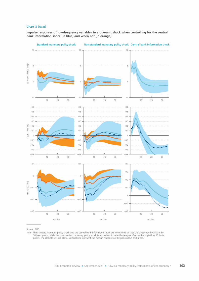
102NBB Economic Review ¡ September 2021 ¡ How do monetary policy instruments affect economy ?
Chart 3 (next)
Impulse responses of low-frequency variables to a one-unit shock when controlling for the central bank information shock (in blue) and when not (in orange)
−5
0
5
10
−5
0
5
10
−5
0
5
10
10 20 3010 20 30 10 20 30
10 20 30 10 20 3010 20 30
10 20 30 10 20 3010 20 30
Standard monetary policy shock Non-standard monetary policy shock Central bank information shock
Euro
stox
x 50
(100
x lo
g)G
DP
(100
x lo
g)
−0.4
−0.3
−0.2
−0.1
0
0.1
0.2
0.3
0.4
0.5
0.6
−0.4
−0.3
−0.2
−0.1
0
0.1
0.2
0.3
0.4
0.5
0.6
−0.4
−0.3
−0.2
−0.1
0
0.1
0.2
0.3
0.4
0.5
0.6
HIC
P (1
00 x
log)
−0.3
−0.2
−0.1
0
0.1
−0.3
−0.2
−0.1
0
0.1
−0.2
−0.1
0
0.1
0.2
0.3
0.4
months monthsmonths
Source : NBB.Note : The standard monetary policy shock and the central bank information shock are normalised to raise the three-month OIS rate by
10 basis points, while the non-standard monetary policy shock is normalised to raise the ten-year German bond yield by 10 basis points. The credible sets are 68 %. Dotted lines represent the median responses of Belgian output and prices.

103NBB Economic Review ¡ September 2021 ¡ How do monetary policy instruments affect economy ?
Conclusion
Estimating the causal effects of monetary policy on the economy is complex. It requires the identification of monetary policy shocks, i.e. policy actions that deviate from the central bank’s usual reaction function. Increases in central banks’ transparency and systematic behaviour in recent decades may have made the identification of standard monetary policy shocks more difficult. In addition, the introduction of non-standard monetary policy measures brought new identification challenges. Research has developed novel identification methods though, providing necessary insight in the financial and macroeconomic effects of new monetary policy tools and how these compare to the effects of standard central bank policy rate changes. With new measures likely to stay, even being considered part of the standard monetary policy toolbox, research on their effects will remain of interest. Further advances in modelling and econometric techniques can only contribute to deepening our understanding of the propagation of monetary policy shocks.
The empirical analysis in this article studied the effects of a tightening in the ECB’s standard policy rate instrument and new measures targeting the long rate (while controlling for central bank information shocks) on the euro area and Belgian economy. To separate the three shocks, a relatively novel identification approach (introduced by Jarociński and Karadi, 2020) was used, combining high-frequency financial market data with sign restrictions in a Bayesian VAR model. Overall, the empirical analysis conducted suggests that non-standard monetary policy measures affect euro area and Belgian macro-economic variables in a rather comparable manner as standard surprises in policy rates.. Results are not always significant, though. The analysis also found that the selection of the high-frequency surprise variable included in the model to clean pure monetary policy shocks for information shocks can be important for identifying the central bank information channel.

104NBB Economic Review ¡ September 2021 ¡ How do monetary policy instruments affect economy ?
Bibliography
Altavilla C., L. Brugnolini, R.S. Gurkaynak, R. Motto, G. Ragusa (2019), “Measuring Euro Area Monetary Policy”, Journal of Monetary Economics, 108, 162 – 179.
Andrade P. and F. Ferroni (2021), “Delphic and odyssean monetary policy shocks : Evidence from the euro area”, Journal of Monetary Economics, 117, 816 – 832.
Bernanke B.S., J. Boivin and P. Eliasz (2005), “Measuring the effects of monetary policy: A factor-augmented vector autoregressive (FAVAR) approach,” Quarterly Journal of Economics, 120 (1), 387 – 422.
BIS (2019), Unconventional monetary policy tools : A cross-country analysis, CGFS Papers, 63.
Blanchard O.J. and D. Quah (1989), “The dynamic effects of aggregate demand and supply disturbances”, The American Economic Review, 79 (4), 655 – 673.
Boeckx J., M. de Sola Perea, M. Deroose, G. de Walque, Th. Lejeune and Ch. Van Nieuwenhuyze (2018), “What will happen when interest rates go up ?”, NBB Economic Review, September, 35 – 56.
Bu C., J. Rogers and W. Wu (2021), “A unified measure of Fed monetary policy shocks”, Journal of Monetary Economics, 118, 331 – 349.
Goodhead R. (2019), The Economic impact of yield curve compression : Evidence from euro area conventional and unconventional monetary policy, Central Bank of Ireland, Economic Letter, 13.
Goodhead R. (2021), The economic impact of yield curve compression: Evidence from euro area forward guidance and unconventional monetary policy, Central Bank of Ireland, Research Technical Paper, 2021 (1).
Hoesch L., B. Rossi, and T. Sekhposyan, (2020), Has the Information Channel of Monetary Policy Disappeared ? Revisiting the Empirical Evidence, CEPR Discussion Paper, 14456.
Jarociński M. and P. Karadi (2020), “Deconstructing monetary policy surprises – The role of information shocks”, American Economic Journal : Macroeconomics, 12 (2), 1 – 43.
Kuttner K.N. (2001), “Monetary policy surprises and interest rates: Evidence from the Fed funds futures market”, Journal of Monetary Economics, 47 (3), 523 – 544.
Laséen S. (2020), Monetary policy surprises, central bank information shocks, and economic activity in a small open economy, Sveriges Riksbank Working Paper Series, 396, October.
Miranda-Agrippino S. and G. Ricco (2021), “The transmission of monetary policy shocks”, American Economic Journal : Macroeconomics, 13 (3), 74 – 107.
Nakamura E. and J. Steinsson (2018), Identification in macroeconomics, NBER, Working Paper 23968, January.
Paul P. (2020) : “The Time-Varying Effect of Monetary Policy on Asset Prices,” The Review of Economics and Statistics, October, 102 (4), 1 – 15.
Ramey V.A. (2016), Macroeconomic Shocks and Their Propagation, NBER, Working Paper 21978, February.

105NBB Economic Review ¡ September 2021 ¡ How do monetary policy instruments affect economy ?
Romer C. and D. Romer (2000), “Federal Reserve Information and the Behavior of Interest Rates”, American Economic Review, 90 (3), 429 – 457.
Romer C. and D. Romer (2004), “A new measure of monetary shocks : Derivation and implications”, American Economic Review, 94 (4), 1055 – 1084.
Rossi B. (2019), Identifying and estimating the effects of unconventional monetary policy in the data : How to do it and what have we learned ?, Barcelona Graduate School of Economics, Working Paper 1081, January.
Rostagno M., C. Altavilla, G. Carboni, W. Lemke, R. Motto and A. Saint Guilhelm (2021), Combining negative rates, forward guidance and asset purchases : Identification and impacts of the ECB’s unconventional policies, ECB, Working Paper Series, 2564, June.
Stock J.H. and M.W. Watson (2016), “Factor Models and Structural Vector Autoregressions”, Chapter 8 in J.B. Taylor and H. Uhlig (eds.), Handbook of Macroeconomics, Elsevier, 415-525.
Taylor J.B. (1993), “Discretion versus policy rules in practice”, Carnegie-Rochester Conference Series on Public Policy, 39, 195 – 214.
Uhlig H. (2005), “What are the effects of monetary policy on output? Results from an agnostic identification procedure”, Journal of Monetary Economics, 52 (2), 381 – 419.