How Do Regulators Influence MortgageRisk: Evidence from an Emerging Market

The Harvard community has made thisarticle openly available. Please share howthis access benefits you. Your story matters

Citation Campbell, John Y., Tarun Ramadorai, and Benjamin Ranish. 2012.How Do Regulators Influence Mortgage Risk? Evidence from anEmerging Market. NBER Working Paper No. 18394, National Bureauof Economic Research.

Published Version doi:10.3386/w18394

Citable link http://nrs.harvard.edu/urn-3:HUL.InstRepos:12168178

Terms of Use This article was downloaded from Harvard University’s DASHrepository, and is made available under the terms and conditionsapplicable to Other Posted Material, as set forth at http://nrs.harvard.edu/urn-3:HUL.InstRepos:dash.current.terms-of-use#LAA

How Do Regulators In�uence Mortgage Risk?

Evidence from an Emerging Market�

John Y. Campbell, Tarun Ramadorai, and Benjamin Ranishy

September 9, 2012

Abstract

To understand the e¤ects of regulation on mortgage risk, it is instructive to trackthe history of regulatory changes in a country rather than to rely entirely on cross-country evidence that can be contaminated by unobserved heterogeneity. However,in developed countries with fairly stable systems of �nancial regulation, it is di¢ cultto track these e¤ects. We employ loan-level data on over a million loans disbursed inIndia over the 1995 to 2010 period to understand how fast-changing regulation impactedmortgage lending and risk. We �nd evidence that regulation has important e¤ects onmortgage rates and delinquencies in both the time-series and the cross-section.

�We gratefully acknowledge an Indian mortgage provider for providing us with the data, and manyemployees of the Indian mortgage provider, Jishnu Das, Jennifer Huang, Ajay Shah, S. Sridhar, UshaThorat, and R. V. Verma for useful conversations and discussions. We thank seminar participants at theEconometric Society/European Economics Association Malaga Conference, the NBER Household FinanceSummer Institute, IIM Bangalore, the World Bank, the Oxford-Man Institute of Quantitative Finance,Saïd Business School, the HKUST Household Finance Symposium, and the NIPFP-DEA Conference onInternational Capital Flows for comments, the International Growth Centre and the Sloan Foundation for�nancial support, and Vimal Balasubramaniam for able research assistance.

yCampbell: Department of Economics, Littauer Center, Harvard University, Cambridge MA 02138, USA,and NBER. Email john_campbell@harvard.edu. Ramadorai: Saïd Business School, Oxford-Man Instituteof Quantitative Finance, University of Oxford, Park End Street, Oxford OX1 1HP, UK, and CEPR. Emailtarun.ramadorai@sbs.ox.ac.uk. Ranish: Department of Economics, Littauer Center, Harvard University,Cambridge MA 02138, USA. Email: branish@fas.harvard.edu.

1 Introduction

How does mortgage regulation in�uence the structure and performance of housing �nance?

This paper answers the question by analyzing administrative data on over 1.2 million loans

originated by an Indian mortgage provider, relating loan pricing and delinquency rates to

the changing details of Indian mortgage regulation.

A more common approach to this question is to compare mortgage systems across coun-

tries. Casual observation reveals striking cross-country di¤erences. A recent survey by the

International Monetary Fund (IMF 2011) shows that among developed countries, homeown-

ership rates range from 43% in Germany to about 80% in southern European countries. The

level of mortgage debt in relation to GDP varies from 22% in Italy to above 100% in Denmark

and the Netherlands. The terms of mortgage instruments are overwhelmingly adjustable-

rate in southern Europe, and �xed-rate in the United States. Mortgages are funded using a

wide variety of mechanisms, including deposit-�nanced lending, mortgage-backed securities,

and covered bonds.

Government involvement in mortgage markets also varies across countries, and it is likely

that this explains at least some of the cross-country variation in housing �nance. However,

it is hard to disentangle regulatory e¤ects from other factors that may a¤ect household

mortgage choice across countries, including historical experiences with interest rate and

in�ation volatility, which can have long-lasting e¤ects because consumers can be slow to

adopt new �nancial instruments (Campbell 2012). An appealing alternative approach is

to trace the e¤ects of mortgage regulation over time within a single country rather than

rely entirely on cross-country evidence that can be contaminated by unobserved di¤erences

across countries. The di¢ culty in doing this is that developed countries tend to have fairly

stable systems of �nancial regulation, so one rarely has the opportunity to track the e¤ects

of sharp regulatory changes. Slow changes, such as those that occurred in the US during

the early and mid-2000s, may well be important but it is hard to show this convincingly.

For this reason academic writers and public policy commentators have reached no consensus

on the degree to which regulation, rather than other factors, caused the US mortgage credit

1

boom.1

Mortgages are rapidly becoming important �nancial instruments in emerging markets.

Here, �nancial regulation is at least as intrusive and much less stable. In addition, long-

lasting historical in�uences are likely to be less important in emerging markets because their

rapid growth and �nancial evolution reduce consumer inertia. For this reason, emerging

markets are ideal laboratories in which to examine the e¤ects of mortgage regulation. How-

ever emerging markets pose a di¤erent challenge, that of �nding adequate data. Many

questions about mortgage �nance can only be answered using microeconomic data, either at

the household level or the loan level. There is now a vast literature looking at such data

in the US, but it is harder to �nd in less wealthy countries with rapidly changing �nancial

systems.2

This paper uses high-quality microeconomic data to study the mortgage market in In-

dia, a large and complex emerging economy. India has been studied extensively by the

economics profession, which has mainly analyzed issues of poverty and development (see,

for example, Besley and Burgess, 2000, and Banerjee et al., 2007), or the impact of the

Byzantine system of laws and regulations on industrial organization and �rm output (see

Aghion et al., 2008, and von Lilienfeld-Toal, Mookherjee, and Visaria, 2012 for example).

India underwent an economic liberalization in the early 1990s and subsequently experienced

rapid economic growth that accelerated further in the 2000s. During this time the �nancial

sector has become much larger and more sophisticated, but remains highly regulated, with a

signi�cantly nationalized banking sector. It is only very recently that authors (for a recent

example see Anagol and Kim, 2012) have begun to study India in the context of �nancial

regulation and its impacts on fast-changing Indian capital markets. The provision of housing

�nance is evolving particularly rapidly (Tiwari and Debata 2008, Verma 2012). Regulatory

1A range of views can be found in Acharya, Richardson, van Nieuwerburgh, and White (2011), Baily(2011), Ellis (2008), International Monetary Fund (2011), and US Treasury and Department of Housing andUrban Development (2011), among other sources.

2Some recent mortgage studies using US microeconomic data include Adelino, Gerardi, and Willen (2009),Agarwal et al (2011), Amromin et al (2011), Bhutta, Dokko, and Shan (2010), Demyanyk and van Hemert(2011), Foote et al (2010), Johnson and Li (2011), Keys et al (2010), Melzer (2011), Mian and Su� (2009),and Piskorski, Seru, and Vig (2011).

2

norms have changed frequently, albeit with a continuing emphasis on funding housing for

low-income households. There is increased competition between mortgage lenders, and this

may have contributed to rapidly increasing house prices since 2002. Indian mortgages in-

clude both �xed and variable rate loans, but there has been a signi�cant shift over time

towards the latter.

We are fortunate to have access to loan-level administrative data from an Indian mortgage

provider. We analyze over 1.2 million mortgages disbursed by the mortgage provider between

1995 and 2010, and attempt to understand both the macroeconomic and microeconomic

determinants of mortgage rate setting and delinquencies. These data reveal three interesting

�ndings which relate regulation to mortgage risk. First, simple plots reveal a signi�cant spike

in delinquencies in the early 2000s. When we estimate a model which relates delinquencies

to demographic information, loan characteristics, and macroeconomic shocks, we �nd that

even after controlling for these determinants, the spike in delinquencies shows up in the

cohort e¤ects for loans issued in those years. We connect these estimated cohort e¤ects

to a number of regulatory changes which encouraged mortgage lending at that time, and

we regard this as strong, albeit circumstantial evidence for regulatory e¤ects on mortgage

defaults.

Second, in addition to this time-series evidence on aggregate mortgage default rates, we

provide evidence on the impacts of regulation from the cross-section of defaults conditioned

on various loan attributes. In particular, throughout the period of study, small and micro

loans are particularly favoured by the Indian regulatory environment. We uncover evidence

that the implicit subsidies to such loans show up in a higher propensity for them to default

than can be accounted for by their mortgage rates at issuance and all other determinants in

the model. This tendency is highly statistically signi�cant, is greater for micro loans than

for small loans just under the subsidy-qualifying threshold, and is observed in all cohorts

of loan issuance over the sample period. We also �nd that the magnitude of the excess

delinquency propensity of small and micro loans appears to vary over time in a way that can

be connected to the tightness of the constraint favoring these loans.

Third, we �nd a signi�cant and somewhat abrupt decline in three-month payment delin-

3

quencies beginning in early 2004. We connect this �nding to the fact that the regulatory

de�nition of �non-performing assets,�a de�nition which is associated with provisioning re-

quirements against such delinquent loans, changes in March 2004, from previously referring

to loans that are six-months delinquent to those that are three-months delinquent. Follow-

ing this change, we �nd that one-month delinquent loans are far less likely to subsequently

become three-months delinquent. Furthermore, using a subsample of 10,000 loans for which

we have a complete time-series of payment histories, we uncover evidence that is consistent

with more e¤ort on the part of the mortgage provider to monitor delinquencies in response

to this regulatory change. In particular, we �nd that debt collection rates on one-month

delinquent loans are accelerated in the interval before they hit the new three-month mark

for classi�cation as a non-performing asset. Importantly, perhaps as a result of incentivizing

mortgage lenders to act early on delinquent loans, we �nd that this change substantially low-

ers the likelihood of experiencing longer-term defaults. This impact on long-term defaults

is even larger than that arising from a 2002 legal change in the ability of mortgage providers

to more easily repossess or restructure non-performing assets.

Taken together, these three �ndings provide compelling evidence that regulatory norms

impact the risk of delinquencies experienced by our Indian mortgage provider on loans issued.

Our evidence complements recent �ndings using U.S. data on the impacts of regulatory norms

on mortgage screening (Keys et al. 2011), and is also related to work on how mortgage credit

expansion in the U.S., particularly in sub-prime zipcodes, contributed to the recent crisis

(Mian and Su� 2009). Our model shows that controlling for a range of determinants of

mortgage risk, the time when a loan is issued has signi�cant explanatory power, a �nding

related to the analysis of Demyanyk and van Hemert (2011) who perform a similar analysis

to explain U.S. sub-prime mortgage risk. Finally, our �ndings are relevant to the suggestion

of Kashyap, Rajan, and Stein (2008) that capital requirements against risk-weighted assets

should be countercyclically adjusted. We �nd that a reduction in the risk-weight on housing

�nance following a period of low GDP growth is associated with high levels of mortgage

delinquencies for loans issued in those cohorts, implying that Kashyap, Rajan, and Stein�s

policy can in�uence the riskiness of mortgage lending.

4

The organization of the paper is as follows. Section 2 sets the stage by describing the

Indian macroeconomic environment over our period of study, the mortgage data that we

employ, and the Indian system of mortgage regulation. Further details on that system are

provided in an online regulatory appendix (Campbell, Ramadorai, and Balasubramaniam

2012). Section 3 introduces our model of mortgage delinquencies, which we use to show

that changing demographic characteristics of borrowers, loan characteristics, or estimated

macro shocks cannot fully explain the high delinquency rate in the early 2000s. Instead,

changing regulation to encourage mortgage lending appears to be responsible. Section 4

presents evidence that regulation has also a¤ected the relative pricing of small and large

mortgages, and discusses the change in the regulatory de�nition of non-performing assets

in 2004 and its consequences on observed delinquency and repayment patterns. Section 5

concludes. Additional empirical evidence on the Indian mortgage market is reported in an

online empirical appendix (Campbell, Ramadorai, and Ranish 2012).

2 The Macroeconomic and Regulatory Environment

2.1 Macroeconomic and Mortgage Finance Trends

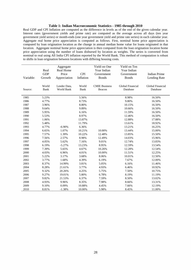
To set the stage, Table 1 illustrates the history of several important macroeconomic variables

over the past quarter-century in India, including annual real GDP growth, CPI in�ation,

and government bond yields. Regulatory and macroeconomic reform in the early 1990s was

followed by growth in the 4-8% range until the early 2000s, when growth accelerated above

8%, brie�y slowed again only by the global �nancial crisis in 2008. Meanwhile in�ation was

high and volatile during the 1990s, with volatility particularly elevated around the reform

period and in 1998�99. A period of more stable in�ation followed in the 2000s, but in�ation

accelerated at the very end of our sample period.

Indian government bond yields over the same period are also quite volatile. The 1-year

yield declines from double-digit levels in the mid-1990s, with considerable volatility in the

late 1990s related to the volatile in�ation experienced at the same time. After a low of

5

about 5% in the early 2000s, the 1-year yield spikes up in 2008, again related to concerns

about in�ation. The 10-year yield is smoother but also undergoes a large decline from the

mid-1990s until the early 2000s.

Figure 1 plots house price indexes, both for India as a whole and for �ve broad regions.

We compute the indexes using the mortgage provider�s own property cost data, but data

from the National Housing Bank (NHB) show similar patterns. Indian house prices were

relatively stable until the early 2000s and then began to increase rapidly, particularly in the

south of the country. The southern index peaks in 2008 while some other regions peak in

2009. Thus India took part in the worldwide housing boom despite many di¤erences in

other aspects of its macroeconomic performance.

Over this same period, the Indian mortgage market was experiencing rapid change. Fig-

ure 2 illustrates one aspect of this change, namely a shift from a predominantly �xed-rate

mortgage system to one that is dominated by variable-rate lending. The �gure plots the

share of variable-rate loans in total issuance by our mortgage provider. Starting at about

40% of dollar value in the mid-1990s, the variable-rate share increases above 90% by the

early 2000s, then brie�y dips to 60% in 2004 before again rising and reaching 100% by the

end of our sample period. The cause of the brief shift back towards �xed-rate mortgages in

2004 is an interesting question that we discuss later in the paper.

Figure 3 plots the delinquency rate (the fraction of mortgages that are 90 days past due),

seasonally adjusted using a regression on monthly dummies, for both �xed-rate mortgages

(solid line) and variable-rate mortgages (dashed line). The main feature of this �gure is a

large spike in delinquencies in 2002�03, particularly for �xed-rate mortgages. This spike

is one of the features of the data that we attempt to explain using our model, which we

introduce in the next section. Delinquencies decline to quite low levels by 2005, and remain

low to the end of our sample period despite the weak housing market in 2009�10.

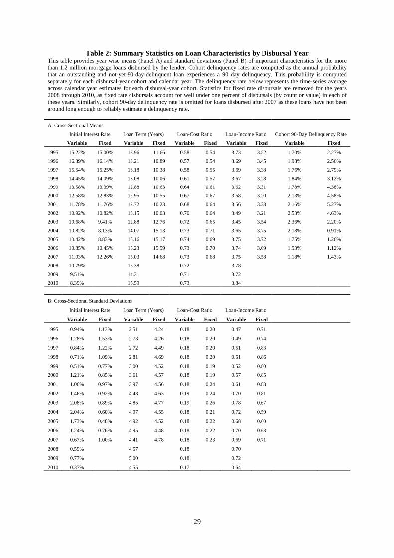
Table 2 shows how our mortgage lender responded to the market conditions described

above. Panel A reports cross-sectional means of mortgage terms and delinquency rates.

Initial interest rates on variable-rate and �xed-rate mortgages track one another very closely

until 2002, and are both close to the Indian prime rate shown in Table 1, despite some

6

variation in the spread between long-term and short-term government yields. In the period

2003�06, the variable mortgage rate is well above the �xed rate and has an unusually high

spread over the 1-year bond yield, a feature shared with the Indian prime rate. This period

has a generally high market share for variable mortgages, but does include the episode in 2004

when our mortgage lender shifted back towards �xed mortgage issuance. Variable mortgage

rates decline after 2008, a period where �xed mortgages have essentially disappeared from

our dataset.

The right-hand column reports the cohort 90-day delinquency rate, the annual probability

that an outstanding and not-yet-delinquent loan experiences a 90-day delinquency, calculated

separately for each disbursal-year cohort and calendar year, and then averaged over calendar

years for each cohort. The early 2000s appear unusual in the sense that the cohort default

rate for mortgages disbursed in these years is high relative to the other cohorts in the

sample period, despite loan characteristics such as loan-to-cost and loan-to-income ratios

not changing much on average. The 2004 cohort, especially for �xed rate loans, however,

appears to have a signi�cantly reduced default rate, which we connect to the spike in �xed

rate issuance later in the paper.

Panel B of Table 2 shows the cross-sectional standard deviation of loan characteristics

and initial interest rates. In the early 2000s there is a large spike in the cross-sectional

dispersion of variable mortgage rates. This spike coincides with the period of increased

delinquencies documented earlier, and may re�ect increased e¤orts by our mortgage lender

to distinguish among borrowers by estimating their default risk and setting mortgage rates

accordingly. For �xed mortgage rates, while the same pattern is not evident in the cross-

sectional dispersion of initial interest rates, there does seem to be an increase in the early

2000s in the cross-sectional dispersion of loan-to-cost ratios, which reduces again in 2004.

In the remainder of this paper, we relate several of the summary statistics described

above to changes in the Indian regulatory environment for housing �nance. Our empirical

work requires a basic understanding of the regulatory structure in India, to which we now

turn.

7

2.2 The Regulatory Environment

Mortgages in India are originated by two types of �nancial institutions, banks and housing

�nance companies (HFCs). Banks are regulated by the Reserve Bank of India (RBI), while

housing �nance companies are regulated by the National Housing Bank (NHB), but most

regulations apply in fairly similar form to the two types of institution. This fact is important

for our study, as we are unable to publicly identify whether our mortgage provider is a bank

or an HFC.

Figure 4 summarizes the details of mortgage regulation in India in a relatively parsimo-

nious fashion. The top half of the �gure shows regulations that applied to banks, and the

bottom half to HFCs. The regulations that remained constant throughout the period are

listed in black, whereas the ones that changed over the period are in colored font. In light

of the signi�cant changes that took place from 2001 to 2002, we separate the timeline into

the ��rst period,� i.e. prior to March 2001, and the �second period�which extends from

April 2001 until the end of the sample period. In the middle of the �gure, we summarize

subsidy schemes for micro-lending with the length of the bars accompanying these schemes

identifying their start and end dates relative to the timeline.

Regulations can be divided into two types: those that restrict the funding of mortgage

lending, and those that incentivize lending to favored borrowers. Until 2001, mortgage

funding was regulated in a fairly traditional manner, using leverage restrictions on banks

and HFCs, and interest-rate ceilings on deposit-taking HFCs. From 2002 onwards, these

measures were augmented by capital requirements against risk-weighted assets following

the internationally standard Basel II framework. The RBI and NHB distinguished small

and large loans, and loan-to-value (LTV) ratios above and below 75%, and set di¤erent risk

weights for these di¤erent categories with frequent changes for loans below 75% LTV. In this

way the regulators shifted the risk capital available to banks and HFCs, and the incentives

for aggressive mortgage origination.

Another noteworthy change in the regulatory environment is highlighted on the timeline,

and occurred on March 31, 2004 for banks, and one year later, i.e., March 31, 2005 for HFCs.

8

At this time the RBI rede�ned an asset as a �non-performing asset�(or NPA) if payments

(on interest or principal) remained overdue for a period of ninety days or more, from the

previous 180 day period allowed before assets were so classi�ed. One important implication

of the classi�cation of an asset as an NPA is that it incurs provisioning requirements, meaning

that the capital available to a mortgage lender holding such an asset reduces as the lender

is required to hold precautionary capital to cover expected losses. Related to this NPA

rede�nition, an important law which came into force in July 2002, also highlighted on the

timeline, was the Securitisation and Reconstruction of Financial Assets and Enforcement

of Security Interest (SARFAESI) Act. This law enabled the easier recovery of NPAs via

securitization, reconstruction, or direct repossession, bypassing the need for secured creditors

to seek permission from debt recovery tribunals (see von Lilienfeld-Toal, Mookherjee, and

Visaria, 2012, for evidence of the impacts of the establishment of these tribunals in 1993). In

our analysis, we separately evaluate the impact of these two changes, namely the rede�nition

of NPAs in 2004, and the introduction of SARFAESI in 2002, on delinquencies experienced

by the mortgage provider.

Lending to small borrowers is an important political goal in India. Banks are subject to a

quantity target for Priority-Sector Lending (PSL), which includes loans to agriculture, small

businesses, export credit, a¢ rmative action lending, educational loans, and �of particular

interest to us �mortgages for low-cost housing. The PSL target is 40% of net bank credit

for domestic banks (32% for foreign banks), and there is a severe �nancial penalty for failure

to meet the target, namely, compulsory lending to rural agriculture at a haircut to the repo

rate. This regulation does not directly apply to HFCs, but bank lending to an HFC quali�es

for the PSL target to the extent that the HFC makes mortgage loans that qualify, i.e., are

below the speci�ed nominal PSL threshold. The overall e¤ect of the PSL system is to

provide a strong incentive, directly for banks, and indirectly for HFCs, to originate small

mortgages that �nance low-cost housing purchases.

In addition to the PSL system, other schemes have been introduced at various points in

time over the sample period to subsidize new or re�nanced micro-lending �i.e., loans of sizes

well below the PSL-qualifying threshold. The mid-section of Figure 4 shows the various

9

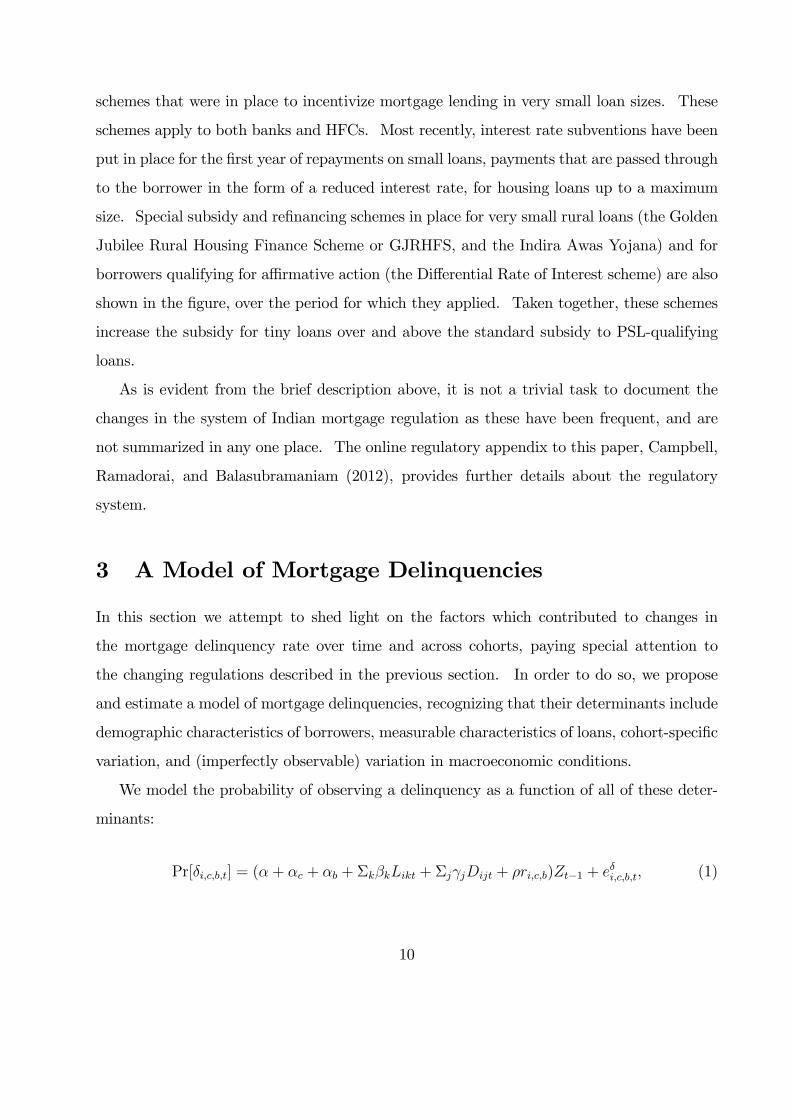
schemes that were in place to incentivize mortgage lending in very small loan sizes. These

schemes apply to both banks and HFCs. Most recently, interest rate subventions have been

put in place for the �rst year of repayments on small loans, payments that are passed through

to the borrower in the form of a reduced interest rate, for housing loans up to a maximum

size. Special subsidy and re�nancing schemes in place for very small rural loans (the Golden

Jubilee Rural Housing Finance Scheme or GJRHFS, and the Indira Awas Yojana) and for

borrowers qualifying for a¢ rmative action (the Di¤erential Rate of Interest scheme) are also

shown in the �gure, over the period for which they applied. Taken together, these schemes

increase the subsidy for tiny loans over and above the standard subsidy to PSL-qualifying

loans.

As is evident from the brief description above, it is not a trivial task to document the

changes in the system of Indian mortgage regulation as these have been frequent, and are

not summarized in any one place. The online regulatory appendix to this paper, Campbell,

Ramadorai, and Balasubramaniam (2012), provides further details about the regulatory

system.

3 A Model of Mortgage Delinquencies

In this section we attempt to shed light on the factors which contributed to changes in

the mortgage delinquency rate over time and across cohorts, paying special attention to

the changing regulations described in the previous section. In order to do so, we propose

and estimate a model of mortgage delinquencies, recognizing that their determinants include

demographic characteristics of borrowers, measurable characteristics of loans, cohort-speci�c

variation, and (imperfectly observable) variation in macroeconomic conditions.

We model the probability of observing a delinquency as a function of all of these deter-

minants:

Pr[�i;c;b;t] = (�+ �c + �b + �k�kLikt + �j jDijt + �ri;c;b)Zt�1 + e�i;c;b;t; (1)

10

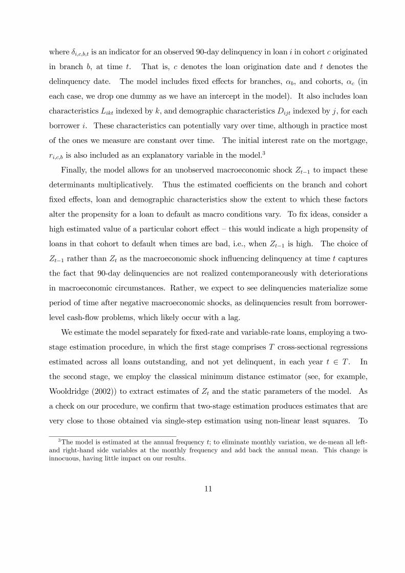
where �i;c;b;t is an indicator for an observed 90-day delinquency in loan i in cohort c originated

in branch b, at time t. That is, c denotes the loan origination date and t denotes the

delinquency date. The model includes �xed e¤ects for branches, �b, and cohorts, �c (in

each case, we drop one dummy as we have an intercept in the model). It also includes loan

characteristics Likt indexed by k, and demographic characteristics Dijt indexed by j, for each

borrower i. These characteristics can potentially vary over time, although in practice most

of the ones we measure are constant over time. The initial interest rate on the mortgage,

ri;c;b is also included as an explanatory variable in the model.3

Finally, the model allows for an unobserved macroeconomic shock Zt�1 to impact these

determinants multiplicatively. Thus the estimated coe¢ cients on the branch and cohort

�xed e¤ects, loan and demographic characteristics show the extent to which these factors

alter the propensity for a loan to default as macro conditions vary. To �x ideas, consider a

high estimated value of a particular cohort e¤ect �this would indicate a high propensity of

loans in that cohort to default when times are bad, i.e., when Zt�1 is high. The choice of

Zt�1 rather than Zt as the macroeconomic shock in�uencing delinquency at time t captures

the fact that 90-day delinquencies are not realized contemporaneously with deteriorations

in macroeconomic circumstances. Rather, we expect to see delinquencies materialize some

period of time after negative macroeconomic shocks, as delinquencies result from borrower-

level cash-�ow problems, which likely occur with a lag.

We estimate the model separately for �xed-rate and variable-rate loans, employing a two-

stage estimation procedure, in which the �rst stage comprises T cross-sectional regressions

estimated across all loans outstanding, and not yet delinquent, in each year t 2 T . In

the second stage, we employ the classical minimum distance estimator (see, for example,

Wooldridge (2002)) to extract estimates of Zt and the static parameters of the model. As

a check on our procedure, we con�rm that two-stage estimation produces estimates that are

very close to those obtained via single-step estimation using non-linear least squares. To

3The model is estimated at the annual frequency t; to eliminate monthly variation, we de-mean all left-and right-hand side variables at the monthly frequency and add back the annual mean. This change isinnocuous, having little impact on our results.

11

obtain standard errors for the second stage estimates we use a cross-sectional correlation

consistent bootstrap procedure, in which we draw a set of time periods equal to the total

number of years (15) in our data t1b ; :::; t15b 2 T with replacement, and assemble a simulated

dataset for each bootstrap draw b. We then re-run the second stage regressions for b = 500

draws.

The demographic variables that we employ include the borrower�s gender, marital status,

number of dependents, and dummies for age (up to age 35, 36-45, and 46 and above), for ed-

ucation (high-school measured by higher-secondary certi�cate or HSC, college, postgraduate,

and missing), for a �nance-related educational quali�cation, and for a repeat borrower. The

loan characteristics include the log loan-to-cost ratio, log loan-to-income ratio, a piecewise

linear function of log loan size in relation to the PSL threshold (discussed in more detail

later in the paper), dummies for origination branch, dummies for whether the loan was paid

by salary deduction or via a special scheme with the employer, as well as dummies for spe-

cial loan characteristics (tranched issuances and re�nancings), speci�c loan purposes (home

extension or improvement), and mortgage contract terms (loan maturities 6-10 years, 11-15

years, or 16 years and above). To control for house-price movements, we also include in the

set of loan characteristics regional house-price appreciation up to time t from the time of the

disbursal of the loan. For variable-rate loans only, we control for the change in the 1-year

Indian government bond yield since issuance. Finally, we include a dummy variable which

takes the value of 1 if a loan is disbursed from a branch in the 12 months prior to a state

election, to capture the possibility (documented by Cole 2009 for Indian agricultural lending)

that in election seasons there may be pressure to disburse politically expedient loans, which

have a higher propensity to be delinquent.

3.1 Regulation and Delinquencies: Time-Series Evidence

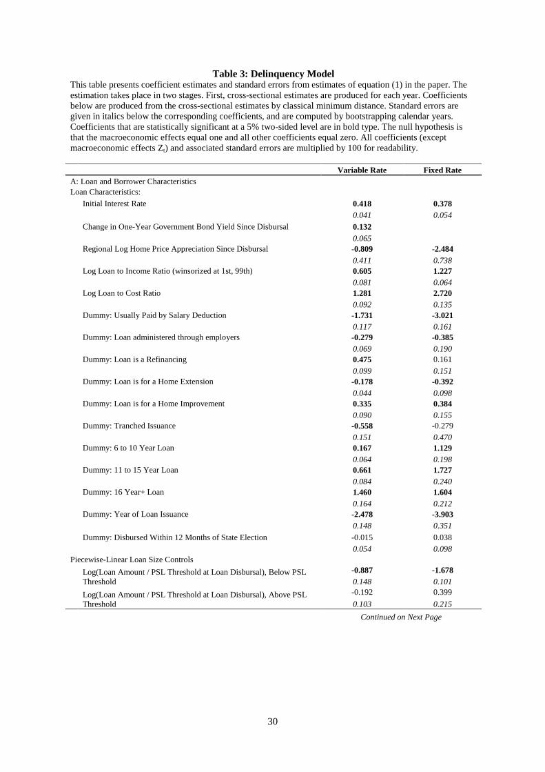
Table 3 shows the estimated coe¢ cients on the demographic and loan characteristics from

equation (1), which predominantly appear to have signs consistent with intuition about

their likely impacts on delinquencies. For the sake of brevity, Table 3 does not present the

12

estimated macroeconomic shocks and cohort e¤ects with associated standard errors, but we

present these in the online empirical appendix (Campbell, Ramadorai, and Ranish 2012).

We do plot these series, however, in Figures 5 and 6.

Figure 5 plots the estimated macroeconomic shocks Zt. Our estimates are weighted by

the relative fractions of �xed and variable rate loan issuance from the separate speci�cations

that we estimate for these two types of loans, a strategy that we continue to adopt in

the remaining �gures in the paper in order to conserve space. The �gure also shows two

di¤erent measures of macroeconomic conditions: real GDP growth, and the average real

rate of growth in corporate sales, �rm �xed assets, and �rm net worth estimated from the

population of Indian �rms available in the Prowess database.4 The �gure, in which all series

are standardized for ease of comparison, shows that estimated Zt seems closely, although not

perfectly related to these other measures. All three measures indicate that 2002 and 2003

were periods of particularly poor macroeconomic conditions, with a complete recovery in the

Indian macro environment only by 2005.

Figure 6 shows how delinquencies vary by their cohort of issuance. The series that we

plot in this �gure is the sum of cohort average �tted values on borrower and loan character-

istics (�hard information�), and the estimated cohort e¤ects from the model (�+ �c) (�soft

information�which is unobservable to the econometrician), again weighted by loan issuance

across �xed and variable rate loans. The bars plotted in the �gure capture the e¤ect of

being issued in a particular year on the delinquency propensity of loans in the sample, after

controlling for macroeconomic shocks.5 The �gure shows that the spike in the delinquency

rate seen in 2002, 2003, and 2004 is connected to loan issuance cohort, not only to prevailing

macroeconomic circumstances in these years.

4This database comprises the population of listed and large unlisted Indian �rms, and is considered tobe the main source of information on Indian corporates (see, for example, von Lilienfeld-Toal, Mookherjee,and Visaria, 2012).

5Note that the estimation of the cohort e¤ects already controls for variation in interest rates at the loanlevel. We also estimate a version of equation (1) in which we replace the interest rate at issuance withthe spread over the one-year Indian government bond yield (in the case of variable-rate loans) or ten-yeargovernment bond yield (in the case of �xed-rate loans). The resulting �gure is presented in the onlineempirical appendix, and is similar to Figure 6, although somewhat noisier because Indian mortgage rates donot move closely with government bond yields, which are therefore an imperfect benchmark.

13

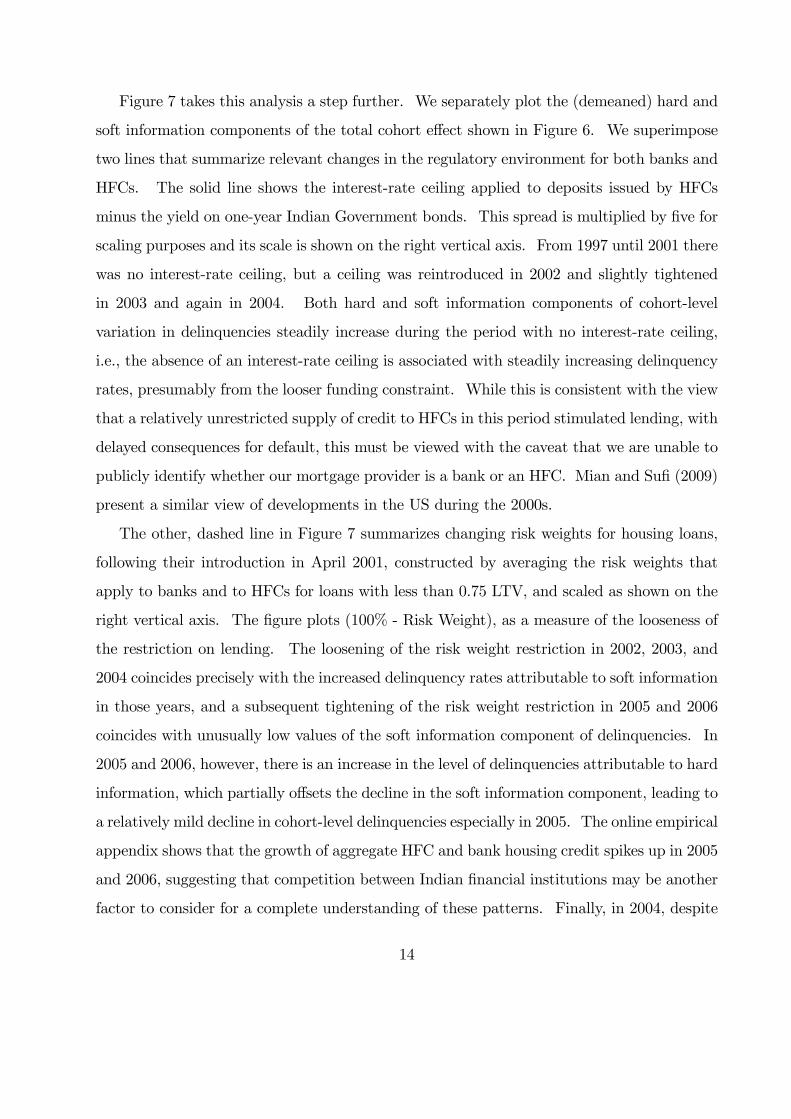
Figure 7 takes this analysis a step further. We separately plot the (demeaned) hard and

soft information components of the total cohort e¤ect shown in Figure 6. We superimpose

two lines that summarize relevant changes in the regulatory environment for both banks and

HFCs. The solid line shows the interest-rate ceiling applied to deposits issued by HFCs

minus the yield on one-year Indian Government bonds. This spread is multiplied by �ve for

scaling purposes and its scale is shown on the right vertical axis. From 1997 until 2001 there

was no interest-rate ceiling, but a ceiling was reintroduced in 2002 and slightly tightened

in 2003 and again in 2004. Both hard and soft information components of cohort-level

variation in delinquencies steadily increase during the period with no interest-rate ceiling,

i.e., the absence of an interest-rate ceiling is associated with steadily increasing delinquency

rates, presumably from the looser funding constraint. While this is consistent with the view

that a relatively unrestricted supply of credit to HFCs in this period stimulated lending, with

delayed consequences for default, this must be viewed with the caveat that we are unable to

publicly identify whether our mortgage provider is a bank or an HFC. Mian and Su�(2009)

present a similar view of developments in the US during the 2000s.

The other, dashed line in Figure 7 summarizes changing risk weights for housing loans,

following their introduction in April 2001, constructed by averaging the risk weights that

apply to banks and to HFCs for loans with less than 0.75 LTV, and scaled as shown on the

right vertical axis. The �gure plots (100% - Risk Weight), as a measure of the looseness of

the restriction on lending. The loosening of the risk weight restriction in 2002, 2003, and

2004 coincides precisely with the increased delinquency rates attributable to soft information

in those years, and a subsequent tightening of the risk weight restriction in 2005 and 2006

coincides with unusually low values of the soft information component of delinquencies. In

2005 and 2006, however, there is an increase in the level of delinquencies attributable to hard

information, which partially o¤sets the decline in the soft information component, leading to

a relatively mild decline in cohort-level delinquencies especially in 2005. The online empirical

appendix shows that the growth of aggregate HFC and bank housing credit spikes up in 2005

and 2006, suggesting that competition between Indian �nancial institutions may be another

factor to consider for a complete understanding of these patterns. Finally, in 2004, despite

14

continued loose risk weight restrictions, the soft information component is slightly lower than

its level in 2003, and we connect this to the shift away from variable-rate to �xed-rate loans

by the mortgage provider �the online empirical appendix plots the cohort e¤ects separately

for �xed and variable loans, and shows that the soft information component of the 2004

cohort e¤ect is relatively lower for �xed-rate loans than for variable-rate loans.

In sum, while one must always be cautious about the interpretation of any pure time-series

correlation, Figure 7 suggests that changes in regulation are an important factor driving the

aggregate delinquency patterns in our data.

4 Regulation and Delinquencies: Cross-Sectional

Evidence

4.1 The E¤ect of Priority Sector Lending Norms

Risk weights and interest rate ceilings are not the only regulatory instruments through

which the Reserve Bank of India a¤ects mortgage lending and risk. Priority-sector lending

(PSL) norms also exist and have cross-sectional e¤ects, diverting lending towards favored

small loans. They do this both through the RBI�s quantity targets for banks, and currently,

through interest-rate subventions for loans up to a certain size. If PSL norms are important,

they might induce mortgage lenders to make riskier loans to small borrowers.

Table 4 presents statistics on the importance of priority-sector lending by our mort-

gage provider, showing the fraction of loan value issued below the prevailing nominal PSL-

qualifying threshold in each year from 1995 to 2010. For variable rate loans, this fraction

declines from roughly 70% in the early years of our sample to 33% in 2010. Micro-loans

(which we classify very simply as those smaller than one-half of the PSL-qualifying threshold)

account for between a third and a little more than a half of the total set of PSL-qualifying

variable rate loan issuance. For �xed rate loans, the fraction of PSL-qualifying loans in

total issuance by value �uctuates between 65% and 85%, with a sharp reduction in 2004 to

48% of total loan issuance. This reduction in 2004, when combined with the lower �xed

15

rate cohort e¤ect in that year which we refer to in the previous section, suggest that the

mortgage provider reduced its reliance on these (potentially more risky) loans in 2004.

Of course, mortgage lenders might make risky small loans in the absence of any regulatory

incentives, if they are able to charge higher mortgage rates to compensate for the higher risk

(Duca and Rosenthal 1994). As a �rst simple way to evaluate whether loans below the PSL

qualifying threshold are riskier even after controlling for mortgage rates, Table 3 allows for

separate slopes for loan sizes above and below the PSL threshold at loan disbursal when

estimating equation (1). If subsidies are responsible for the relationship between loan size

and the propensity to be delinquent, then the slope below the PSL threshold should be

estimated to be negative and statistically signi�cant, because as we know from Figure 4,

there are additional subsidies for micro-lending at loan sizes well below the PSL threshold.

However, there should be no consistent relationship between loan size and the propensity to

be delinquent for loan sizes above the PSL-qualifying threshold.

Table 3 shows that indeed, for loans below the PSL threshold, loan size has a substantial

and statistically signi�cant negative e¤ect on the propensity for a loan to be delinquent.

However, above the PSL-qualifying threshold, while there is a small and marginally statis-

tically signi�cant negative slope estimated for variable rate loans (roughly one-�fth the size

of the slope below the threshold), the slope is small, positive and marginally statistically

signi�cant for �xed rate loans. We view this as evidence that the PSL subsidy distorts the

e¢ cient-market relationship between interest rates and delinquencies, and that loans below

the PSL-qualifying threshold are riskier than those above it.

The negative slope below the PSL-qualifying threshold suggests that micro-loans (i.e.,

those well below the PSL-qualifying threshold) are even riskier than those just below the

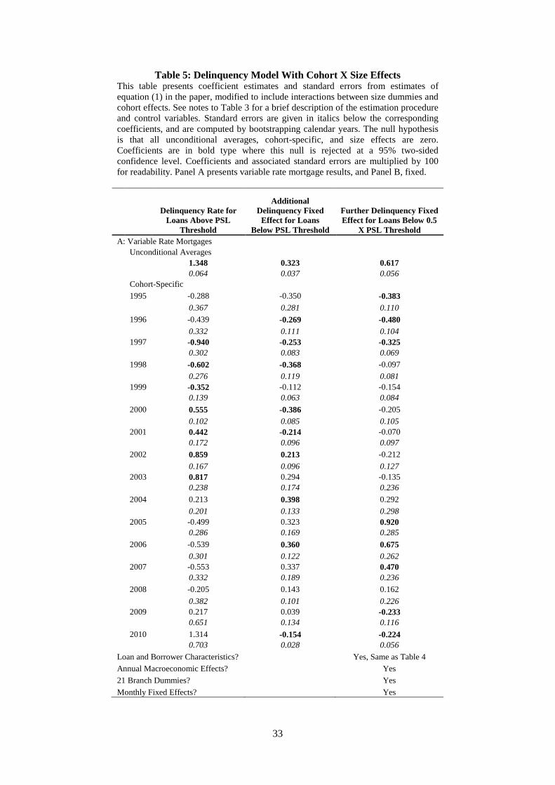
threshold. To evaluate the relative riskiness of di¤erent loan sizes, we estimate a version

of equation (1) in which we interact the cohort e¤ects with two dummy variables, the �rst

of which identi�es whether a loan is below the PSL-qualifying threshold at the time it is

made, and the second which identi�es whether a loan is below one-half the PSL-qualifying

threshold at the time it is made (this is to identify the impact of being a micro loan).

Table 5 shows the estimated unconditional mean and cohort e¤ects (cohort-speci�c de-

16

viations from the unconditional mean) interacted with the size dummies from this model.

Panel A reports results for variable-rate mortgages, and panel B for �xed-rate mortgages.

The table reveals several interesting patterns. First, the probability of being delinquent

is far higher on average for PSL-qualifying and micro loans than for those above the PSL-

qualifying threshold. Second, there is an interesting time pattern to these cohort e¤ects.

Figure 8 plots the excess delinquency propensity over non-subsidized loans in each cohort

(combining the unconditional mean and the cohort e¤ect) for both PSL-qualifying and mi-

cro loans. Variable-rate and �xed-rate cohort e¤ects are weighted by the issuance of each

type of mortgage. In every one of the cohort-years in the data, micro loans have a far

higher propensity to be delinquent, and PSL-qualifying loans also have a higher propensity

in every cohort-year except 1998. There is an interesting U-shaped pattern in these excess

propensities, that is, they are higher at the very beginning of the sample period, decreasing

in the late 1990s, and then increasing from roughly the middle of the sample period until

the end of the sample period.

We overlay two measures of the tightness of the PSL constraint in each cohort-year on

this plot. The �rst is the negative of the (log) ratio of the nominal PSL-qualifying threshold

de�ated by house price appreciation. The PSL-qualifying threshold is increased periodically,

and when it is raised by more than the increase in house prices, the constraint is e¤ectively

looser. Conversely, if the PSL-qualifying threshold remains at the same nominal level when

house prices rise substantially, the constraint is more binding. The second measure tracks

the tightness of the PSL constraint by subtracting aggregate credit extended to the priority

sector by public sector banks, Indian private sector banks, and foreign banks operating in

India from the mandatory PSL lending requirement of these institutions. If more than the

mandatory amount of PSL credit is extended by banks, this revealed preference for PSL

lending suggests that the constraint is less binding, and vice versa.

Figure 8 shows that the pattern of excess PSL delinquency propensities trends upwards

but also roughly tracks the tightness of the PSL constraint. During the late 1990s, excess

delinquency propensities were declining as the PSL constraint became less binding, while

during the 2000s excess delinquency propensities trended up as rising house prices tightened

17

the PSL constraint. To interpret these results, one should keep in mind two points. First,

results for the last few years of the sample period may be distorted by the fact that recent

loans may not yet have experienced delinquencies by the end of the sample period. Second,

as Table 4 shows, while still substantial, PSL-qualifying loans are a smaller fraction of the

mortgage book in the late 2000s.

Nevertheless, we do conclude that there is substantial evidence that small subsidized loans

have delinquency risk over and above larger unsubsidized loans which cannot be accounted for

by their interest rates. This e¤ect appears to vary with the tightness of the PSL constraint,

although overall, the excess default propensities appear to have been increasing over time.

4.2 Change in the Classi�cation of Non-Performing Assets

The discussion on regulation earlier noted another relevant change that took place over the

sample period that we consider: on March 31, 2004 for banks, and March 31, 2005 for HFCs,

the classi�cation of �non-performing asset�(or NPAs) was changed to 90 days past due from

the previous time period of 180 days past due. This regulatory reclassi�cation of 90-day

delinquencies, and the associated implications of this change for provisioning requirements

may also have contributed to the unusually low delinquency rates seen in Figure 7 for more

recent loan cohorts. Of course, this also raises the important question of whether our

previous results using 90-day delinquencies are con�rmed using data on 180-day delinquencies

�a plausible model of behavior is that a mortgage provider might care more about �o¢ cial�

NPAs (rather than delinquencies of a shorter term than the regulatory minimum) as these

have tangible balance sheet implications. Another important question that arises here is

whether the regulatory re-classi�cation of NPAs had other impacts on behavior such as an

increased emphasis on monitoring shorter-term delinquencies (say 30 days past due), as any

reduction in the minimum delinquency period might be expected to feed through to the

earlier monitoring of mortgage default risk.

To answer the �rst of these questions, we re-estimate the model with 180-day delinquen-

cies on the left-hand side replacing 90-day delinquencies. The online empirical appendix

18

to the paper shows that while, as we might have expected, the average delinquency rate is

lower when we consider 180-day delinquencies, the pattern of the cohort-time �xed e¤ects

is consistent with that found using 90-day loans. This provides reassurance that our ear-

lier results are not simply driven by the use of a variable that is perhaps less immediately

important (prior to 2004-5) to the mortgage provider.

To answer the second question, we evaluate the expected loss given a delinquency before

and after the regulatory reclassi�cation. This expected loss is the product of the proba-

bility of experiencing a delinquency and the loss given delinquency. Table 6 looks at the

�rst of these two elements, computing transition probabilities of loans that hit the 30-day

delinquency threshold to the 90-day delinquency mark, as well as the transition probability

of 90-day delinquencies to the 180-day delinquent mark. The table shows that across the

entire sample period, 22.7% (22.8%) of 30-day (90-day) delinquent loans eventually become

90 days (180 days) delinquent.

As we are unable to publicly identify whether the mortgage provider is a bank or an HFC,

we use the earlier RBI implementation date of 31 March 2004 as the date of the regulatory

change, to cover all possibilities. When we look separately at the pre-April 2004 period

for the 30-day delinquencies, the transition probability is 29%, which is almost twice as

high as the post-March 2004 transition probability of 14.9%, and the reduction, of 14.1% is

highly statistically signi�cant. Clearly, following the change in the de�nition of NPAs to the

shorter 90-day limit, the mortgage provider substantially reduced this transition probability,

potentially by exerting e¤ort to pursue borrowers more aggressively. The 90-day to 180-day

transition probability also reduces following the 2004 reclassi�cation, but by a much smaller

2.3%, suggesting that once the loan becomes classi�ed as an NPA, there are relatively fewer

incentives to take action. Another possibility, of course, is that the loans reaching the 90-day

delinquency mark are simply very di¢ cult to collect on despite exertions of e¤ort.6

6It is also worth noting here that the 2002 implementation of SARFAESI, described above, allowed foreasier restructuring and repossession of delinquent loans. However the small change in the 90-180 daytransition probability despite this regulatory change mirrors the insigni�cant post-SARFAESI change in the�CID debt collection rate that we de�ne and analyze below. These results suggest that at least for housingloans, this particular regulatory change may not have had very large e¤ects.

19

To better understand the magnitude of loss given delinquency, we acquire a sample of

10,000 loans from the total population of loans. As our focus is to understand the determi-

nants of mortgage risk, we randomly sample 2,500 �xed-rate and 2,500 variable-rate loans

from the set of 90-day delinquent loans, and a further 2,500 �xed-rate and 2,500 variable-rate

loans from the set of loans that do not experience a 90-day delinquency. In each sub-sample

of 2,500 loans, we further ensure that we sample an equal number (1,250) from the early

period in the data (disbursed prior to January 2000) and the later period (disbursed between

January 2000 and December 2004). The online empirical appendix (Campbell, Ramadorai,

and Ranish 2012) veri�es that this 10,000 loan sample has statistically indistinguishable

characteristics from the population of loans from which we draw. For each one of these

10,000 loans, we are able to track the full payment history over time, as well as deviations

from contracted repayments. We can compute the latter as we are also given the equated

monthly installment (EMI) for each of these loans in each month, which is the expected

monthly principal repayment plus interest amount. We ensure that we weight any measures

constructed using this sample, so that they are re�ective of the larger population of loans

from which the sampling occurred.

For each loan in the sample, we construct a measure of losses accrued over time. To do

so, we accumulate payments and EMI over time, and compute the �cumulative installment

de�cit�(or CID) as Min(0, cumulative payment-cumulative EMI)/EMI. This measure takes

the value of zero if monthly payments exceed or equal the EMI, and is negative otherwise,

indicating when borrowers are in arrears. The cumulation ensures that if overpayments are

made to redress arrears, these are allowed to push the measure towards zero. The division

by EMI puts the cumulative installment de�cit into units of required monthly payments.

Figure 9 plots the CID measure around 30-day delinquencies, before and after the regu-

latory change to the de�nition of NPAs. The measure is cross-sectionally demeaned by both

cohort-year and calendar-year, to ensure that we are not picking up cohort or macroeconomic

e¤ects. In both panels of Figure 9, date 0 is the �rst date that the loan is declared 30-days

delinquent (values below 1 are possible because of the cross-sectional demeaning). The top

panel shows that prior to the change in the regulatory de�nition of NPAs, loans declared

20

30-days delinquent on average in�icted a cost on the mortgage provider of roughly 1.2 EMIs

after a year. Post-March 2004, there is a substantial recovery in this number, with such

30-delinquent loans roughly 0.2 EMIs delinquent 12 months later. The bottom panel of the

�gure shows that this change in the behavior of the CID after the regulatory rede�nition of

NPAs is highly statistically signi�cant.

We undertake this analysis more formally by estimating how changes in the CID vary

following a 30-day delinquency, but prior to hitting the 90-day threshold, both before and

after the regulatory rede�nition of the NPA period. To do so, we estimate expected debt

collection rates � changes in the CID �as a polynomial function of the level of the CID

prior to the 90-day delinquency mark (i.e., a CID level of �3), allowing for a jump in the

rate at the 90-day delinquency mark, and modelled as a linear function of the CID beyond

the 90-day delinquency mark. As before, we include time- and cohort-speci�c �xed e¤ects

during estimation to ensure that we are not merely picking up some of the broader changes

detected earlier in the regulatory and macroeconomic environment.

Figure 10 shows how the estimated debt collection rate varies before and after the 90-

day delinquency threshold, before and after the regulatory rede�nition of NPAs in March

2004. The �gure clearly reveals that following the regulatory rede�nition of NPAs, the debt

collection rate prior to hitting the 90-day mark increased substantially relative to the pre-

regulatory change period, with a signi�cant discontinuity at the 90-day threshold, where the

debt collection rate falls sharply.7 We also consider whether the introduction of SARFAESI

had any signi�cant impacts on the ability to collect on debts, and �nd that while there is

a mild increase in the pre-90 day debt collection rate, it is dwarfed by the change following

the NPA rede�nition (moreover, the small discontinuity evident in this line at the 90-day

mark is statistically insigni�cant).

While these changes to debt collection rates are clearly evident in the data, one potential

worry is that the rede�nition of NPAs from 180 to 90 days simply shifted the inevitable

7The increase in the debt collection rate prior to the 90-day delinquency mark, and the discontinuityat that mark are both economically and statistically signi�cant. The online empirical appendix plotsthe di¤erence between the pre- and post- NPA rede�nition debt collection rates with associated bootstrapcon�dence intervals.

21

recovery of cash from delinquent borrowers by the 90-day di¤erence between these two dates.

In other words, perhaps the change merely provided a time-value improvement in the net

cash �ows of the mortgage provider, but no more substantial impacts.

To address this question, Figure 11 shows the cumulative distribution function (CDF) of

the change in the CID (time- and cohort-demeaned) in the year following the �rst 30 day

delinquency. This CDF is plotted for three time periods, namely, January 1995 to June

2002, when SARFAESI was �rst implemented; July 2002 to March 2004, the date of the

rede�nition of NPAs; and post-April 2004 until the end of the sample period in 2010. We

plot the �gure on a log scale to focus attention on the very worst cases (i.e., those loans with

the greatest degradation in CID over the year following the date of �rst 30-day delinquency),

as these loans are the most likely candidates for a complete write-o¤.

The �gure shows that the post-NPA rede�nition CDF �rst-order stochastically dominates

both the pre- and post-SARFAESI CDFs, showing a substantial reduction in the incidence

of high degradation in the CID. While SARFAESI appears to have had some bene�cial

impacts for the very worst cases, this is dwarfed by the large impact of the NPA rede�nition.

These substantial impacts on eventual bad debts of this regulatory rede�nition are striking,

as it appears that there are important real bene�ts to incentivizing mortgage providers to

detect and take early action on delinquencies.

Taken together, a simple change in the regulatory de�nition of NPAs to a shorter length

of delinquency appears to have generated signi�cant impacts on the expected loss given

delinquency of the mortgage provider. The impacts appear to be felt in reductions in the

probability of delinquency, as well as in the eventual loss given delinquency, and strongly

suggest a signi�cant change in mortgage provider behavior in relation to borrowers in arrears.

While it is di¢ cult to generalize �ndings from one country, these results do suggest that

even seemingly innocuous changes in regulatory de�nitions can have important impacts on

mortgage risk.

22

5 Conclusion

The Indian regulatory and macroeconomic environment has changed dramatically during

the last two decades. A fast-developing housing �nance system has coped with signi�cant

variation in default rates and interest rates, and regulatory changes in the incentives to

originate mortgages in general, and small loans in particular. We have presented evidence

that regulation may have contributed to a surge in delinquencies during the early 2000s, that

subsidies for low-cost housing distorted the e¢ cient markets relationship between interest

rates and subsequent delinquencies, and that changes to the de�nition of non-performing

assets impacted behavior in response to early evidence of payment delinquencies. Our paper

contributes to the growing body of literature on the impacts of regulators and regulatory

norms on risks in �nancial markets.

23

References

Acharya, Viral V., Matthew Richardson, Stijn van Nieuwerburgh, and Lawrence J. White,

2011, Guaranteed to Fail: Fannie Mae, Freddie Mac, and the Debacle of Mortgage

Finance, Princeton University Press, Princeton, NJ.

Adelino, Manuel, Kristopher Gerardi, and Paul S. Willen, 2009, �Renegotiating Home

Mortgages: Evidence from the Subprime Crisis�, unpublished paper, Federal Reserve

Bank of Boston.

Agarwal, Sumit, Gene Amromin, Itzhak Ben-David, Souphala Chomsisengphet, and Dou-

glas D. Evano¤, 2011, �The Role of Securitization in Mortgage Renegotiation�, Dice

Center Working Paper 2011-2, Ohio State University.

Aghion, Philippe, Robin Burgess, Stephen J. Redding, and Fabrizio Zilibotti, 2008, �The

Unequal E¤ects of Liberalization: Evidence from Dismantling the License Raj in In-

dia�, American Economic Review, 98(4), 1397�1412.

Amromin, Gene, Jennifer Huang, Clemens Sialm, and Edward Zhong, 2011, �Complex

Mortgages,� unpublished paper, Federal Reserve Bank of Chicago and University of

Texas at Austin.

Anagol, Santosh, and Hugh Kim, 2012, �The Impact of Shrouded Fees: Evidence from a

Natural Experiment in the Indian Mutual Funds Market�, American Economic Review,

102(1), 576-593.

Baily, Martin N., 2011, ed., The Future of Housing Finance: Restructuring the U.S. Resi-

dential Mortgage Market, Brookings Institution Press, Washington, DC.

Banerjee, Abhijeet, Shawn Cole, Esther Du�o, and Leigh Linden, 2007, �Remedying Edu-

cation: Evidence from Two Randomized Experiments in India,�Quarterly Journal of

Economics, 122(3), 1235-1264.

24

Besley, Tim, and Robin Burgess, 2000, �Land Reform, Poverty Reduction and Growth:

Evidence from India�, Quarterly Journal of Economics, 115 (2), 389-430.

Bhutta, Neil, Jane Dokko, and Hui Shan, 2010, �The Depth of Negative Equity and Mort-

gage Default Decisions,�FEDS Working Paper 2010-35, Federal Reserve Board.

Campbell, John Y., 2012, �Mortgage Market Design�, unpublished paper, Harvard Univer-

sity.

Campbell, John Y., Tarun Ramadorai, and Vimal Balasubramaniam, 2012, �Prudential

Regulation of Housing Finance in India 1995-2011�, regulatory appendix, available at:

http://intranet.sbs.ox.ac.uk/tarun_ramadorai/TarunPapers/PrudentialRegulationAppendix.pdf.

Campbell, John Y., Tarun Ramadorai, and Benjamin Ranish, 2012, �Appendix to Camp-

bell, Ramadorai, and Ranish�, empirical appendix, available at:

http://intranet.sbs.ox.ac.uk/tarun_ramadorai/TarunPapers/MortgageEmpiricalAppendix.pdf.

Campbell, Tim S. and J. Kimball Dietrich, 1983, �The Determinants of Default on Insured

Conventional Residential Mortgage Loans�, Journal of Finance 38, 1569�1581.

Cole, Shawn A., 2009, �Fixing Market Failures or Fixing Elections? Elections, Banks and

Agricultural Lending in India�, American Economic Journal: Applied Economics 1,

219�50.

Demyanyk, Yuliya, and Otto van Hemert, 2011, �Understanding the Subprime Mortgage

Crisis�, Review of Financial Studies, 24, 1848-1880.

Duca, John V. and Stuart S. Rosenthal, 1994, �Do Mortgage Rates Vary Based on House-

hold Default Characteristics? Evidence Based on Rate Sorting and Credit Rationing�,

Journal of Real Estate Finance and Economics 8, 99�113.

Ellis, Luci, 2008, �The Housing Meltdown: Why Did It Happen in the United States?�,

Bank for International Settlements Working Paper 259.

25

Foote, Christopher, Kristopher Gerardi, Lorenz Goette, and Paul Willen, 2010, �Reducing

Foreclosures: No Easy Answers,�NBER Macroeconomics Annual 2009, 89�138.

Hunt, Stefan, 2010, �Informed Traders and Convergence to Market E¢ ciency: Evidence

from a New Commodity Futures Exchange�, unpublished paper, Harvard University.

International Monetary Fund, 2011, �Housing Finance and Financial Stability �Back to

Basics?�, Chapter 3 inGlobal Financial Stability Report, April 2011: Durable Financial

Stability �Getting There from Here, International Monetary Fund, Washington, DC.

Johnson, Kathleen W. and Geng Li, 2011, �Are Adjustable-Rate Mortgage Borrowers Bor-

rowing Constrained?�, FEDS Working Paper 2011-21, Federal Reserve Board, Wash-

ington, DC.

Kashyap, Anil, Raghuram Rajan, and Jeremy Stein, 2008,�Rethinking Capital Regulation�,

in Federal Reserve Bank of Kansas City Symposium on Maintaining Stability in a

Changing Financial System, 431-471.

Keys, Benjamin, Tanmoy Mukherjee, Amit Seru, and Vikrant Vig, 2010, �Did Securitiza-

tion Lead to Lax Screening? Evidence from Subprime Loans�, Quarterly Journal of

Economics 125, 307�362.

von Lilienfeld-Toal, Dilip Mookherjee and Sujata Visaria, 2012, �The Distributive Impact

of Reforms in Credit Enforcement: Evidence from Indian Debt Recovery Tribunals�,

Econometrica, 89, 497-558.

Melzer, Brian T., 2011, �Mortgage Debt Overhang: Reduced Investment by Homeowners

with Negative Equity�, unpublished paper, Northwestern University.

Mian, Atif and Amir Su�, 2009, �The Consequences of Mortgage Credit Expansion: Evi-

dence from the U.S. Mortgage Default Crisis�, Quarterly Journal of Economics 124,

1449�1496.

26

Piskorski, Tomasz, Amit Seru, and Vikrant Vig, 2011, �Securitization and Distressed Loan

Renegotiation: Evidence from the Subprime Mortgage Crisis�, Journal of Financial

Economics 97, 369�397.

Tiwari, Piyush and Pradeep Debata, 2008, �Mortgage Market in India�, Chapter 2 in

Danny Ben-Shahar, Charles Ka Yui Leung, and Seow Eng Ong eds. Mortgage Markets

Worldwide, Blackwell.

U.S. Treasury and Department of Housing and Urban Development, 2011, Reforming Amer-

ica�s Housing Market: A Report to Congress, Washington, DC.

Verma, R.V., 2012, �Evolution of the Indian Housing Finance System and Housing Market�,

Chapter 14 in Ashok Bardhan, Robert H. Edelstein, and Cynthia A. Kroll eds. Global

Housing Markets: Crises, Policies, and Institutions, John Wiley.

Wooldridge, Je¤rey M., 2002, Econometric Analysis of Cross Section and Panel Data, MIT

Press, Cambridge, MA.

27

28

Table 1: Indian Macroeconomic Statistics - 1985 through 2010Real GDP and CPI Inflation are computed as the difference in levels as of the end of the given calendar year.Interest rates (government yields and prime rate) are computed as the average across all days (ten yeargovernment yield series) or month-ends (one year government yield and prime rate series) in each calendar year.Aggregate real home price appreciation is computed as follows. First, nominal home price appreciation iscomputed by loan origination location as the change in annual median home value for loans originated in thatlocation. Aggregate nominal home price appreciation is then computed from the loan origination location homeprice appreciation using the number of loans disbursed by location as weights. The series is converted fromnominal to real using All India CPI inflation reported by the World Bank. This method of computation is robustto shifts in loan origination between locations with differing housing costs.

Variable:

RealGDP

Growth

AggregateReal Home

PriceAppreciation

CPIInflation

Yield on OneYear IndianGovernment

Bonds

Yield on TenYear IndianGovernment

BondsIndian PrimeLending Rate

Source:WorldBank

Lender Data,World Bank

WorldBank

CMIE BusinessBeacon

Global FinancialDatabase

Global FinancialDatabase

1985 5.23% 5.56% 8.98% 16.50%

1986 4.77% 8.73% 9.80% 16.50%

1987 3.96% 8.80% 10.15% 16.50%

1988 9.64% 9.89% 10.66% 16.50%

1989 5.95% 6.16% 11.59% 16.50%

1990 5.53% 8.97% 12.46% 16.50%

1991 1.06% 13.87% 12.88% 17.88%

1992 5.48% 11.79% 13.61% 18.92%

1993 4.77% -6.90% 6.36% 13.21% 16.25%

1994 6.65% 1.07% 10.21% 10.00% 13.44% 15.00%

1995 7.57% 1.39% 10.22% 12.48% 13.85% 15.50%

1996 7.56% 2.57% 8.98% 12.49% 14.03% 15.96%

1997 4.05% 5.62% 7.16% 9.01% 12.74% 13.83%

1998 6.19% -5.27% 13.23% 8.95% 12.59% 13.54%

1999 7.39% 5.65% 4.67% 10.26% 12.28% 12.54%

2000 4.03% 6.96% 4.01% 10.00% 11.51% 12.25%

2001 5.22% 3.17% 3.68% 8.06% 10.01% 12.50%

2002 3.77% 1.68% 4.39% 6.19% 7.67% 12.00%

2003 8.37% 14.99% 3.81% 5.05% 6.16% 11.46%

2004 8.28% 21.61% 3.77% 4.93% 6.46% 10.92%

2005 9.32% 20.26% 4.25% 5.75% 7.50% 10.75%

2006 9.27% 19.01% 5.80% 6.78% 8.19% 11.19%

2007 9.82% 21.53% 6.37% 7.59% 8.50% 13.02%

2008 4.93% 9.96% 8.35% 7.98% 8.66% 13.31%

2009 9.10% 0.09% 10.88% 4.45% 7.66% 12.19%

2010 8.81% -1.38% 10.00% 5.98% 8.45% 11.00%

29

Table 2: Summary Statistics on Loan Characteristics by Disbursal YearThis table provides year wise means (Panel A) and standard deviations (Panel B) of important characteristics for the morethan 1.2 million mortgage loans disbursed by the lender. Cohort delinquency rates are computed as the annual probabilitythat an outstanding and not-yet-90-day-delinquent loan experiences a 90 day delinquency. This probability is computedseparately for each disbursal-year cohort and calendar year. The delinquency rate below represents the time-series averageacross calendar year estimates for each disbursal-year cohort. Statistics for fixed rate disbursals are removed for the years2008 through 2010, as fixed rate disbursals account for well under one percent of disbursals (by count or value) in each ofthese years. Similarly, cohort 90-day delinquency rate is omitted for loans disbursed after 2007 as these loans have not beenaround long enough to reliably estimate a delinquency rate.

A: Cross-Sectional Means

Initial Interest Rate Loan Term (Years) Loan-Cost Ratio Loan-Income Ratio Cohort 90-Day Delinquency Rate

Variable Fixed Variable Fixed Variable Fixed Variable Fixed Variable Fixed

1995 15.22% 15.00% 13.96 11.66 0.58 0.54 3.73 3.52 1.70% 2.27%

1996 16.39% 16.14% 13.21 10.89 0.57 0.54 3.69 3.45 1.98% 2.56%

1997 15.54% 15.25% 13.18 10.38 0.58 0.55 3.69 3.38 1.76% 2.79%

1998 14.45% 14.09% 13.08 10.06 0.61 0.57 3.67 3.28 1.84% 3.12%

1999 13.58% 13.39% 12.88 10.63 0.64 0.61 3.62 3.31 1.78% 4.38%

2000 12.58% 12.83% 12.95 10.55 0.67 0.67 3.58 3.20 2.13% 4.58%

2001 11.78% 11.76% 12.72 10.23 0.68 0.64 3.56 3.23 2.16% 5.27%

2002 10.92% 10.82% 13.15 10.03 0.70 0.64 3.49 3.21 2.53% 4.63%

2003 10.68% 9.41% 12.88 12.76 0.72 0.65 3.45 3.54 2.36% 2.20%

2004 10.82% 8.13% 14.07 15.13 0.73 0.71 3.65 3.75 2.18% 0.91%

2005 10.42% 8.83% 15.16 15.17 0.74 0.69 3.75 3.72 1.75% 1.26%

2006 10.85% 10.45% 15.23 15.59 0.73 0.70 3.74 3.69 1.53% 1.12%

2007 11.03% 12.26% 15.03 14.68 0.73 0.68 3.75 3.58 1.18% 1.43%

2008 10.79% 15.38 0.72 3.78

2009 9.51% 14.31 0.71 3.72

2010 8.39% 15.59 0.73 3.84

B: Cross-Sectional Standard Deviations

Initial Interest Rate Loan Term (Years) Loan-Cost Ratio Loan-Income Ratio

Variable Fixed Variable Fixed Variable Fixed Variable Fixed

1995 0.94% 1.13% 2.51 4.24 0.18 0.20 0.47 0.71

1996 1.28% 1.53% 2.73 4.26 0.18 0.20 0.49 0.74

1997 0.84% 1.22% 2.72 4.49 0.18 0.20 0.51 0.83

1998 0.71% 1.09% 2.81 4.69 0.18 0.20 0.51 0.86

1999 0.51% 0.77% 3.00 4.52 0.18 0.19 0.52 0.80

2000 1.21% 0.85% 3.61 4.57 0.18 0.19 0.57 0.85

2001 1.06% 0.97% 3.97 4.56 0.18 0.24 0.61 0.83

2002 1.46% 0.92% 4.43 4.63 0.19 0.24 0.70 0.81

2003 2.08% 0.89% 4.85 4.77 0.19 0.26 0.78 0.67

2004 2.04% 0.60% 4.97 4.55 0.18 0.21 0.72 0.59

2005 1.73% 0.48% 4.92 4.52 0.18 0.22 0.68 0.60

2006 1.24% 0.76% 4.95 4.48 0.18 0.22 0.70 0.63

2007 0.67% 1.00% 4.41 4.78 0.18 0.23 0.69 0.71

2008 0.59% 4.57 0.18 0.70

2009 0.77% 5.00 0.18 0.72

2010 0.37% 4.55 0.17 0.64

30

Table 3: Delinquency ModelThis table presents coefficient estimates and standard errors from estimates of equation (1) in the paper. Theestimation takes place in two stages. First, cross-sectional estimates are produced for each year. Coefficientsbelow are produced from the cross-sectional estimates by classical minimum distance. Standard errors aregiven in italics below the corresponding coefficients, and are computed by bootstrapping calendar years.Coefficients that are statistically significant at a 5% two-sided level are in bold type. The null hypothesis isthat the macroeconomic effects equal one and all other coefficients equal zero. All coefficients (exceptmacroeconomic effects Zt) and associated standard errors are multiplied by 100 for readability.

Variable Rate Fixed Rate

A: Loan and Borrower Characteristics

Loan Characteristics:

Initial Interest Rate 0.418 0.378

0.041 0.054

Change in One-Year Government Bond Yield Since Disbursal 0.132

0.065

Regional Log Home Price Appreciation Since Disbursal -0.809 -2.484

0.411 0.738

Log Loan to Income Ratio (winsorized at 1st, 99th) 0.605 1.227

0.081 0.064

Log Loan to Cost Ratio 1.281 2.720

0.092 0.135

Dummy: Usually Paid by Salary Deduction -1.731 -3.021

0.117 0.161

Dummy: Loan administered through employers -0.279 -0.385

0.069 0.190

Dummy: Loan is a Refinancing 0.475 0.161

0.099 0.151

Dummy: Loan is for a Home Extension -0.178 -0.392

0.044 0.098

Dummy: Loan is for a Home Improvement 0.335 0.384

0.090 0.155

Dummy: Tranched Issuance -0.558 -0.279

0.151 0.470

Dummy: 6 to 10 Year Loan 0.167 1.129

0.064 0.198

Dummy: 11 to 15 Year Loan 0.661 1.727

0.084 0.240

Dummy: 16 Year+ Loan 1.460 1.604

0.164 0.212

Dummy: Year of Loan Issuance -2.478 -3.903

0.148 0.351

Dummy: Disbursed Within 12 Months of State Election -0.015 0.038

0.054 0.098

Piecewise-Linear Loan Size Controls

Log(Loan Amount / PSL Threshold at Loan Disbursal), Below PSLThreshold

-0.887 -1.678

0.148 0.101

Log(Loan Amount / PSL Threshold at Loan Disbursal), Above PSLThreshold

-0.192 0.399

0.103 0.215

Continued on Next Page

31

Variable Rate Fixed Rate

Borrower Characteristics:

Log Number of Dependents -0.114 0.225

0.046 0.066

Male Borrower 0.182 0.492

0.027 0.059

Married Borrower 0.042 0.149

0.042 0.091

Borrower age 36-45 0.080 0.116

0.013 0.059

Age 46 and up 0.227 0.221

0.044 0.075

Dummy: Repeat Borrower 0.425 0.850

0.117 0.135

Dummy: Qualification Missing or Unidentified -0.125 -0.142

0.068 0.084

Dummy: HSC Equivalent -0.396 -0.857

0.074 0.082

Dummy: BA Equivalent -0.633 -1.241

0.104 0.089

Dummy: Post-Grad Equivalent -1.016 -1.796

0.098 0.109

Dummy: Finance-Related Qualification 0.177 0.209

0.028 0.064

Cohort Fixed Effects? Yes, Appendix Table A1

Annual Macroeconomic Effects? Yes, Appendix Table A1

21 Branch Dummies? Yes

Monthly Fixed Effects? Yes

32

Table 4: Share of Loan Disbursals Above and Below Priority Sector Lending (PSL) Threshold Values

The share of loan disbursals above and below the PSL threshold and 0.5 times the PSL threshold are given as the share of the total value of loans disbursed in the given year. The PSL thresholdlevels are sporadically reset (October 22, 1997, October 29, 1999, April 29, 2003, October 26, 2004, and July 2, 2007 are reset dates between 1995 and 2010). The regulatory source documentsare detailed in the online regulatory appendix. The distribution of fixed rate mortgage issuances after 2007 is not shown due to the limited extent of fixed rate lending in these years.

Variable Rate Share of Disbursals Variable Rate Mortgages Fixed Rate Mortgages

By Count By Value Above PSL Threshold Below PSL Threshold Below 0.5X PSL Threshold Above PSL Threshold Below PSL Threshold Below 0.5X PSL Threshold

1995 37.86% 42.98% 31.60% 68.40% 30.29% 29.01% 70.99% 37.78%

1996 47.45% 51.78% 36.95% 63.05% 27.07% 35.89% 64.11% 32.08%

1997 55.29% 60.84% 40.09% 59.91% 24.43% 38.27% 61.73% 30.39%

1998 59.04% 66.78% 26.67% 73.33% 40.06% 20.91% 79.09% 49.65%

1999 65.55% 71.32% 27.79% 72.21% 37.43% 21.80% 78.20% 45.77%

2000 75.70% 81.65% 23.36% 76.64% 47.66% 16.58% 83.42% 59.91%

2001 75.32% 82.31% 28.05% 71.95% 42.50% 17.49% 82.51% 61.95%

2002 84.40% 89.83% 32.52% 67.48% 39.23% 15.49% 84.51% 64.97%

2003 94.14% 94.16% 34.44% 65.56% 38.51% 34.88% 65.12% 40.57%

2004 84.51% 79.97% 35.35% 64.65% 34.28% 51.60% 48.40% 21.43%

2005 90.40% 92.09% 37.43% 62.57% 33.57% 24.81% 75.19% 45.40%

2006 90.44% 92.87% 56.03% 43.97% 21.21% 35.09% 64.91% 34.43%

2007 95.76% 97.72% 59.76% 40.24% 17.10% 35.61% 64.39% 39.08%

2008 99.44% 99.80% 60.32% 39.68% 15.53%

2009 99.87% 99.97% 64.58% 35.42% 13.19%

2010 99.97% 99.99% 66.72% 33.28% 9.69%

33

Table 5: Delinquency Model With Cohort X Size EffectsThis table presents coefficient estimates and standard errors from estimates ofequation (1) in the paper, modified to include interactions between size dummies andcohort effects. See notes to Table 3 for a brief description of the estimation procedureand control variables. Standard errors are given in italics below the correspondingcoefficients, and are computed by bootstrapping calendar years. The null hypothesisis that all unconditional averages, cohort-specific, and size effects are zero.Coefficients are in bold type where this null is rejected at a 95% two-sidedconfidence level. Coefficients and associated standard errors are multiplied by 100for readability. Panel A presents variable rate mortgage results, and Panel B, fixed.

Delinquency Rate forLoans Above PSL

Threshold

AdditionalDelinquency Fixed

Effect for LoansBelow PSL Threshold

Further Delinquency FixedEffect for Loans Below 0.5

X PSL Threshold

A: Variable Rate Mortgages

Unconditional Averages

1.348 0.323 0.617

0.064 0.037 0.056

Cohort-Specific

1995 -0.288 -0.350 -0.383

0.367 0.281 0.110

1996 -0.439 -0.269 -0.480

0.332 0.111 0.104

1997 -0.940 -0.253 -0.325

0.302 0.083 0.069

1998 -0.602 -0.368 -0.097

0.276 0.119 0.081

1999 -0.352 -0.112 -0.154

0.139 0.063 0.084

2000 0.555 -0.386 -0.205

0.102 0.085 0.105

2001 0.442 -0.214 -0.070

0.172 0.096 0.097

2002 0.859 0.213 -0.212

0.167 0.096 0.127

2003 0.817 0.294 -0.135

0.238 0.174 0.236

2004 0.213 0.398 0.292

0.201 0.133 0.298

2005 -0.499 0.323 0.9200.286 0.169 0.285

2006 -0.539 0.360 0.675

0.301 0.122 0.262

2007 -0.553 0.337 0.470

0.332 0.189 0.236

2008 -0.205 0.143 0.162

0.382 0.101 0.226

2009 0.217 0.039 -0.2330.651 0.134 0.116

2010 1.314 -0.154 -0.2240.703 0.028 0.056

Loan and Borrower Characteristics? Yes, Same as Table 4

Annual Macroeconomic Effects? Yes

21 Branch Dummies? Yes

Monthly Fixed Effects? Yes

34

Table 5: Delinquency Model With Cohort X Size Effects (Contd.)Panel B: Fixed rate mortgages. Cohort effects from 2008 through 2010 are ignored asthe limited number of fixed rate issuances in these years makes estimation ofassociated cohort effects imprecise.

Delinquency Rate forLoans Above PSL

Threshold

AdditionalDelinquency Fixed

Effect for LoansBelow PSL Threshold

Further Delinquency FixedEffect for Loans Below 0.5

X PSL Threshold

B: Fixed Rate Mortgages

Unconditional Averages, 1995-2007

2.075 0.397 1.310

0.169 0.086 0.112

Cohort-Specific

1995 -1.103 -0.056 -0.200

0.805 0.299 0.224

1996 -0.816 -0.186 -0.020

0.737 0.297 0.283

1997 -0.591 -0.272 -0.150

0.706 0.195 0.209

1998 -0.088 -0.582 -0.202

0.734 0.393 0.184

1999 0.214 -0.548 -0.053

0.667 0.168 0.294

2000 0.179 0.216 0.025

0.587 0.401 0.198

2001 1.758 -0.242 -0.055

0.601 0.498 0.451

2002 2.077 0.513 0.089

1.129 0.787 0.577

2003 0.773 0.318 0.048

0.772 0.261 0.548

2004 -0.167 0.522 -0.534

0.820 0.291 0.288

2005 -0.709 0.217 0.664

0.760 0.184 0.507

2006 -0.928 0.165 0.145

0.732 0.244 0.518

2007 -0.599 -0.066 0.244

0.676 0.496 0.788

Loan and Borrower Characteristics? Yes, Same as Table 4

Annual Macroeconomic Effects? Yes

21 Branch Dummies? Yes

Monthly Fixed Effects? Yes

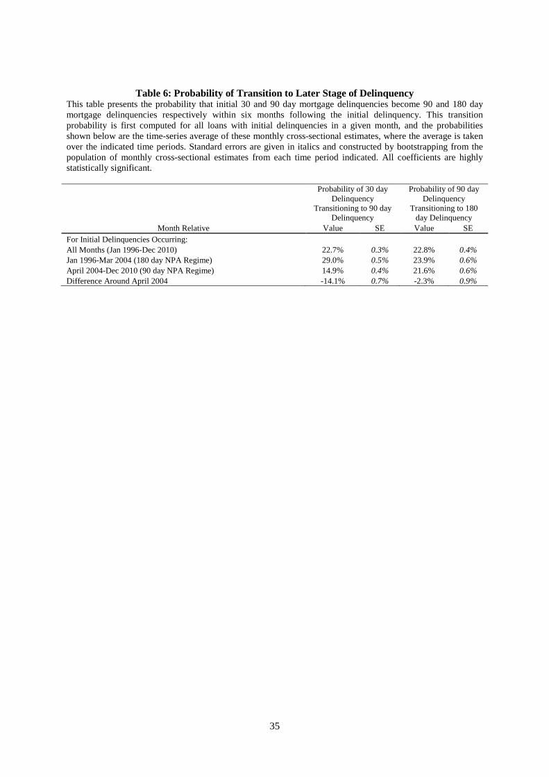
35

Table 6: Probability of Transition to Later Stage of DelinquencyThis table presents the probability that initial 30 and 90 day mortgage delinquencies become 90 and 180 daymortgage delinquencies respectively within six months following the initial delinquency. This transitionprobability is first computed for all loans with initial delinquencies in a given month, and the probabilitiesshown below are the time-series average of these monthly cross-sectional estimates, where the average is takenover the indicated time periods. Standard errors are given in italics and constructed by bootstrapping from thepopulation of monthly cross-sectional estimates from each time period indicated. All coefficients are highlystatistically significant.

Probability of 30 dayDelinquency

Transitioning to 90 dayDelinquency

Probability of 90 dayDelinquency

Transitioning to 180day Delinquency

Month Relative Value SE Value SE

For Initial Delinquencies Occurring:

All Months (Jan 1996-Dec 2010) 22.7% 0.3% 22.8% 0.4%Jan 1996-Mar 2004 (180 day NPA Regime) 29.0% 0.5% 23.9% 0.6%

April 2004-Dec 2010 (90 day NPA Regime) 14.9% 0.4% 21.6% 0.6%

Difference Around April 2004 -14.1% 0.7% -2.3% 0.9%

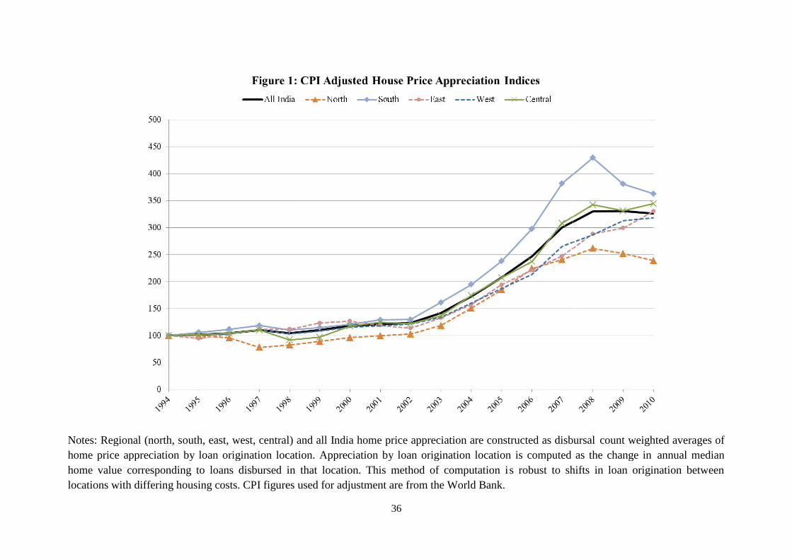
Notes: Regional (north, south, east, west, central) and all India home price appreciation are constructed as disbursal

home price appreciation by loan origination location. Appreciation by loan origination location is computed as the change in

home value corresponding to loans disbursed in that location. This method of computation i

locations with differing housing costs. CPI figures used for adjustment are from the World Bank.

36

Regional (north, south, east, west, central) and all India home price appreciation are constructed as disbursal

home price appreciation by loan origination location. Appreciation by loan origination location is computed as the change in

home value corresponding to loans disbursed in that location. This method of computation is robust to shifts in loan origination between

locations with differing housing costs. CPI figures used for adjustment are from the World Bank.

Regional (north, south, east, west, central) and all India home price appreciation are constructed as disbursal count weighted averages of

home price appreciation by loan origination location. Appreciation by loan origination location is computed as the change in annual median

s robust to shifts in loan origination between

37

Notes: Seasonal adjustments are computed by regressing log quarterly 90 day delinquency rates (for all ou

mortgages) on a set of year and calendar quarter dummies. The calendar quarter dummies from the log default rate regressions

exponentiated, normalized to one, and are used as scaling factors to seasonally

delinquency rates (DEFQ) are annualized by the transformation 1

38

Seasonal adjustments are computed by regressing log quarterly 90 day delinquency rates (for all ou

mortgages) on a set of year and calendar quarter dummies. The calendar quarter dummies from the log default rate regressions

exponentiated, normalized to one, and are used as scaling factors to seasonally-adjust the quarterly delinquency rates. The resulting quarterly

delinquency rates (DEFQ) are annualized by the transformation 1-(1-DEFQ)4.

Seasonal adjustments are computed by regressing log quarterly 90 day delinquency rates (for all outstanding fixed or variable rate

mortgages) on a set of year and calendar quarter dummies. The calendar quarter dummies from the log default rate regressions are

rterly delinquency rates. The resulting quarterly

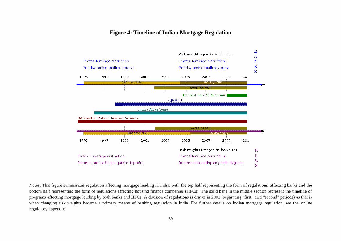
Figure

Notes: This figure summarizes regulation affecting mortgage lending in India, with the top half representing the form of regulations

bottom half representing the form of regulations affecting housing finance companies (HFCs). The solid bar

programs affecting mortgage lending by both banks and HFCs. A division of regulations is drawn in 2001 (separating "first" an

when changing risk weights became a primary means

regulatory appendix

39

igure 4: Timeline of Indian Mortgage Regulation

This figure summarizes regulation affecting mortgage lending in India, with the top half representing the form of regulations

bottom half representing the form of regulations affecting housing finance companies (HFCs). The solid bar s in the middle section represent the timeline of

programs affecting mortgage lending by both banks and HFCs. A division of regulations is drawn in 2001 (separating "first" an

when changing risk weights became a primary means of banking regulation in India. For further details on Indian mortgage regulation, see the

This figure summarizes regulation affecting mortgage lending in India, with the top half representing the form of regulations affecting banks and the

s in the middle section represent the timeline of

programs affecting mortgage lending by both banks and HFCs. A division of regulations is drawn in 2001 (separating "first" an d "second" periods) as that is

of banking regulation in India. For further details on Indian mortgage regulation, see the online

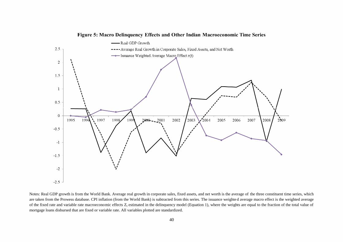
Notes: Real GDP growth is from the World Bank. Average real growth in corporate sales, fixed assets, and net worth is the average of

are taken from the Prowess database. CPI inflation (from the World Bank) is subtracted from this series. The issuance weighte

of the fixed rate and variable rate macroeconomic effects Z

mortgage loans disbursed that are fixed or variable rate. All variables plotted are standardized.

40

Real GDP growth is from the World Bank. Average real growth in corporate sales, fixed assets, and net worth is the average of

are taken from the Prowess database. CPI inflation (from the World Bank) is subtracted from this series. The issuance weighte d average macro effect is the weighted average

mic effects Zt estimated in the delinquency model (Equation 1), where the weights are equal to the fraction of the total value of

mortgage loans disbursed that are fixed or variable rate. All variables plotted are standardized.

Real GDP growth is from the World Bank. Average real growth in corporate sales, fixed assets, and net worth is the average of the three constituent time series, which

d average macro effect is the weighted average

estimated in the delinquency model (Equation 1), where the weights are equal to the fraction of the total value of

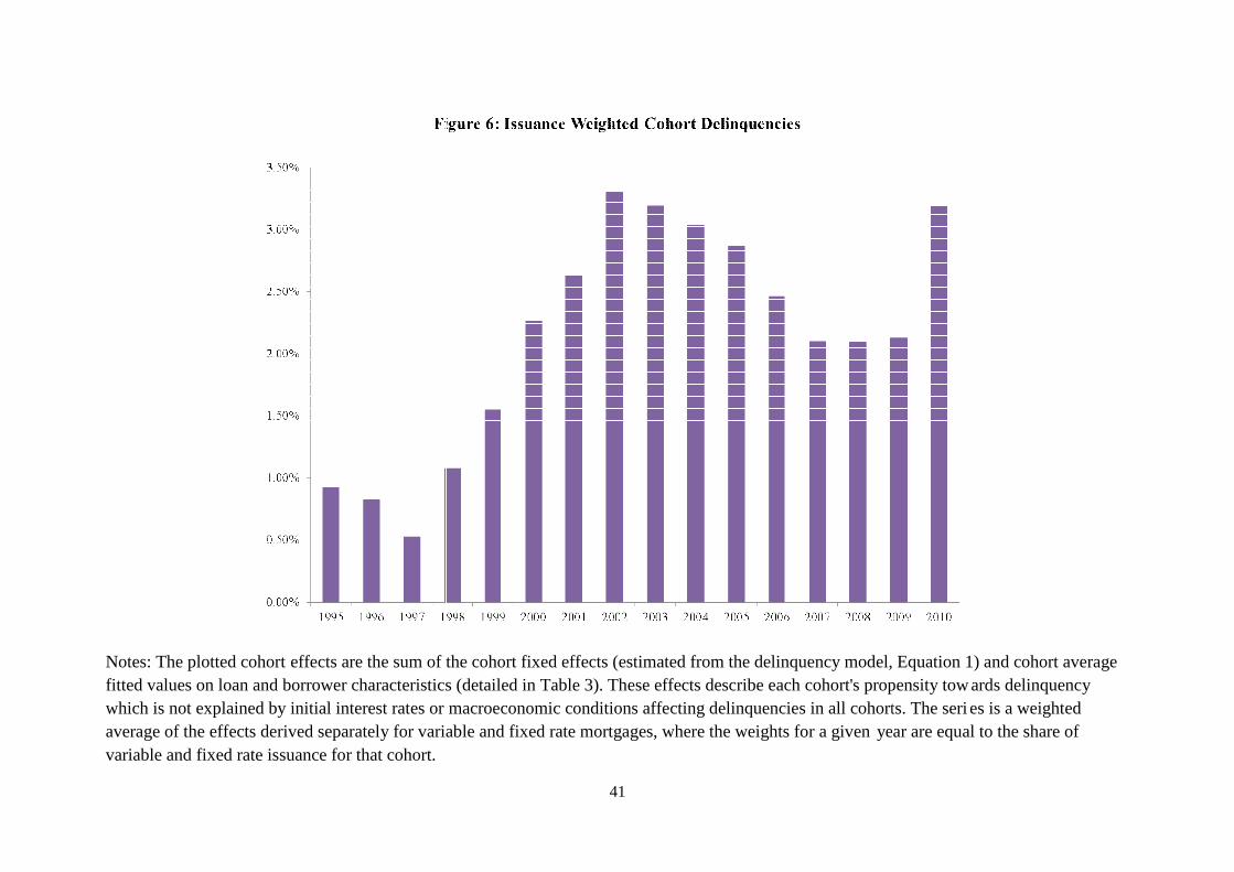
Notes: The plotted cohort effects are the sum of the cohort fixed effects (estimated from the delinquency model, Equation 1) and cohort average

fitted values on loan and borrower characteristics (detailed in Table 3). These effects describe each cohort's propensity tow

which is not explained by initial interest rates or macroeconomic conditions affecting delinquencies in all cohorts. The seri

average of the effects derived separately for variable and fixed rate mortgages, where the weights for a given

variable and fixed rate issuance for that cohort.

41

effects are the sum of the cohort fixed effects (estimated from the delinquency model, Equation 1) and cohort average

fitted values on loan and borrower characteristics (detailed in Table 3). These effects describe each cohort's propensity tow

which is not explained by initial interest rates or macroeconomic conditions affecting delinquencies in all cohorts. The seri

average of the effects derived separately for variable and fixed rate mortgages, where the weights for a given year are equal to the share of

effects are the sum of the cohort fixed effects (estimated from the delinquency model, Equation 1) and cohort average

fitted values on loan and borrower characteristics (detailed in Table 3). These effects describe each cohort's propensity tow ards delinquency

which is not explained by initial interest rates or macroeconomic conditions affecting delinquencies in all cohorts. The seri es is a weighted

year are equal to the share of

Notes: The plotted cohort effects are a decomposition of the de

attributed to loan and borrower attributes (cohort average fitted values from the delinquency model) and (2) soft information

other cohort effects (cohort fixed effects in the delinquency model). The interest rate ceiling is a maximum interest rate that housing fina

allowed to pay to depositors. Risk weights are used to determine capital requirements for banks and HFCs, with hi

capital provisioning. The risk weight series is the average of the risk weights applicable to banks and HFCs lending where lo

such risk weights change in the middle of a year, each r

42

The plotted cohort effects are a decomposition of the de-meaned abnormal cohort delinquencies in Figure 6 into (1) hard information

attributed to loan and borrower attributes (cohort average fitted values from the delinquency model) and (2) soft information

fects (cohort fixed effects in the delinquency model). The interest rate ceiling is a maximum interest rate that housing fina

allowed to pay to depositors. Risk weights are used to determine capital requirements for banks and HFCs, with hi gher risk weight assets requiring greater

capital provisioning. The risk weight series is the average of the risk weights applicable to banks and HFCs lending where lo

such risk weights change in the middle of a year, each risk weight is weighted by the fraction of the year for which it was applicable.

abnormal cohort delinquencies in Figure 6 into (1) hard information - delinquencies

attributed to loan and borrower attributes (cohort average fitted values from the delinquency model) and (2) soft information - delinquencies attributed to

fects (cohort fixed effects in the delinquency model). The interest rate ceiling is a maximum interest rate that housing fina nce companies are

gher risk weight assets requiring greater

capital provisioning. The risk weight series is the average of the risk weights applicable to banks and HFCs lending where lo an-to-value is below 0.75. Where

isk weight is weighted by the fraction of the year for which it was applicable.

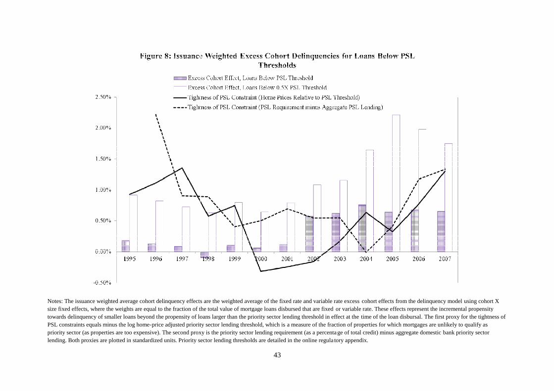
Notes: The issuance weighted average cohort delinquency effects are the weighted average of the fixed rate and variable rate excess

size fixed effects, where the weights are equal to the fraction of the total value of mortgage loans disbursed that are fixed

towards delinquency of smaller loans beyond the propensity of loans larger than the priority sector lending threshold in effect at the

PSL constraints equals minus the log home-price adjusted priority sector lending threshold, which is

priority sector (as properties are too expensive). The second proxy is the priority sector lending requirement (as a percenta

lending. Both proxies are plotted in standardized units. Priority sector lending thresholds are detailed in the online regula

43

The issuance weighted average cohort delinquency effects are the weighted average of the fixed rate and variable rate excess cohort effects from the delinquency model

size fixed effects, where the weights are equal to the fraction of the total value of mortgage loans disbursed that are fixed or variable rate. These effects represent the incremental propensity

he propensity of loans larger than the priority sector lending threshold in effect at the time of the loan disbursal.

price adjusted priority sector lending threshold, which is a measure of the fraction of properties for which mortgages are unlikely to qualify as

priority sector (as properties are too expensive). The second proxy is the priority sector lending requirement (as a percentage of total credit) minus aggregate domestic

lending. Both proxies are plotted in standardized units. Priority sector lending thresholds are detailed in the online regula tory appendix.

cohort effects from the delinquency model using cohort X

or variable rate. These effects represent the incremental propensity

time of the loan disbursal. The first proxy for the tightness of

a measure of the fraction of properties for which mortgages are unlikely to qualify as

ge of total credit) minus aggregate domestic bank priority sector

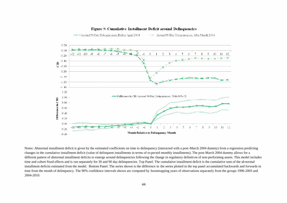
Notes: Abnormal installment deficit is given by the estimated coefficients on time to delinquency (interacted with a post

changes in the cumulative installment deficit (value of delinquent installments in terms of ex

different pattern of abnormal installment deficits to emerge around delinquencies following the change in regulatory definiti

time and cohort fixed effects and is run separately for 30 and 90 day delinquencies. Top Panel: The cumulative installment deficit is the cumulative sum of the ab

installment deficits estimated from the model. Bottom Panel: The series shown is the difference in

time from the month of delinquency. The 90% confidence intervals shown are computed by

2004-2010.

44

Abnormal installment deficit is given by the estimated coefficients on time to delinquency (interacted with a post -March 2004 dummy) from a regression predicting

changes in the cumulative installment deficit (value of delinquent installments in terms of expected monthly installments). The post-March 2004 dummy allows for a

different pattern of abnormal installment deficits to emerge around delinquencies following the change in regulatory definiti on of non-

run separately for 30 and 90 day delinquencies. Top Panel: The cumulative installment deficit is the cumulative sum of the ab

installment deficits estimated from the model. Bottom Panel: The series shown is the difference in the series plotted in the top panel accumulated backwards and forwards in

time from the month of delinquency. The 90% confidence intervals shown are computed by bootstrapping years of observations separately from the groups 1996

March 2004 dummy) from a regression predicting

March 2004 dummy allows for a

-performing assets. This model includes

run separately for 30 and 90 day delinquencies. Top Panel: The cumulative installment deficit is the cumulative sum of the ab normal

accumulated backwards and forwards in

ately from the groups 1996-2003 and

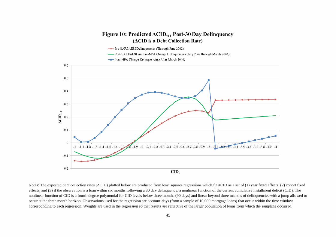
Notes: The expected debt collection rates (ΔCID) plotted below are produced from least squares regressions which fit ΔCID as a set o

effects, and (3) if the observation is a loan within six months following a 30 da

nonlinear function of CID is a fourth degree polynomial for CID levels below three months (90 days) and linear beyond three m

occur at the three month horizon. Observations used for the regression are account

corresponding to each regression. Weights are used in the regression so that results

45

The expected debt collection rates (ΔCID) plotted below are produced from least squares regressions which fit ΔCID as a set of (1) year fixed effects, (2) cohort fixed

effects, and (3) if the observation is a loan within six months following a 30 day delinquency, a nonlinear function of the current cumulative installment deficit (CID). The

nonlinear function of CID is a fourth degree polynomial for CID levels below three months (90 days) and linear beyond three months of delinquencies with a jump all

occur at the three month horizon. Observations used for the regression are account-days (from a sample of 10,000 mortgage loans) that occur within the time window

corresponding to each regression. Weights are used in the regression so that results are reflective of the larger population of loans from which the sampling occurred.

f (1) year fixed effects, (2) cohort fixed

y delinquency, a nonlinear function of the current cumulative installment deficit (CID). The

onths of delinquencies with a jump allowed to

days (from a sample of 10,000 mortgage loans) that occur within the time window

are reflective of the larger population of loans from which the sampling occurred.

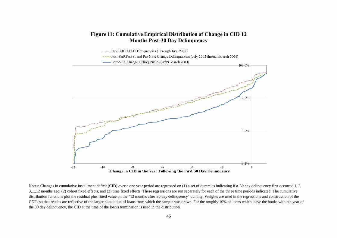
Notes: Changes in cumulative installment deficit (CID) over a one year period are regressed on (1) a set of dummies indicating if a

3,...,12 months ago, (2) cohort fixed effects, and (3) time fixed effects. These regressions are run separately for each of the thr

distribution functions plot the residual plus fitted value on the "12 months after

CDFs so that results are reflective of the larger population of loans from which the sample was drawn. For the roughly 10% of

the 30 day delinquency, the CID at the time of the loan's termination is used in the distribution.

46

Changes in cumulative installment deficit (CID) over a one year period are regressed on (1) a set of dummies indicating if a 30 day delinquency first occurred 1, 2,

12 months ago, (2) cohort fixed effects, and (3) time fixed effects. These regressions are run separately for each of the thr ee time periods indicated. The cumulative

distribution functions plot the residual plus fitted value on the "12 months after 30 day delinquency" dummy. Weights are used in the regressions and construction of the

CDFs so that results are reflective of the larger population of loans from which the sample was drawn. For the roughly 10% of loans which leave the books within a year

the 30 day delinquency, the CID at the time of the loan's termination is used in the distribution.

30 day delinquency first occurred 1, 2,

ee time periods indicated. The cumulative

30 day delinquency" dummy. Weights are used in the regressions and construction of the

loans which leave the books within a year of