DI

SC

US

SI

ON

P

AP

ER

S

ER

IE

S

Forschungsinstitut zur Zukunft der ArbeitInstitute for the Study of Labor

How Deep Is Your Love? A Quantitative Spatial Analysis of the Transatlantic Trade Partnership

IZA DP No. 9021

April 2015

Oliver KrebsMichael Pflüger

How Deep Is Your Love?

A Quantitative Spatial Analysis of the Transatlantic Trade Partnership

Oliver Krebs University of Würzburg

Michael Pflüger University of Würzburg,

DIW Berlin and IZA

Discussion Paper No. 9021 April 2015

IZA

P.O. Box 7240 53072 Bonn

Germany

Phone: +49-228-3894-0 Fax: +49-228-3894-180

E-mail: iza@iza.org

Any opinions expressed here are those of the author(s) and not those of IZA. Research published in this series may include views on policy, but the institute itself takes no institutional policy positions. The IZA research network is committed to the IZA Guiding Principles of Research Integrity. The Institute for the Study of Labor (IZA) in Bonn is a local and virtual international research center and a place of communication between science, politics and business. IZA is an independent nonprofit organization supported by Deutsche Post Foundation. The center is associated with the University of Bonn and offers a stimulating research environment through its international network, workshops and conferences, data service, project support, research visits and doctoral program. IZA engages in (i) original and internationally competitive research in all fields of labor economics, (ii) development of policy concepts, and (iii) dissemination of research results and concepts to the interested public. IZA Discussion Papers often represent preliminary work and are circulated to encourage discussion. Citation of such a paper should account for its provisional character. A revised version may be available directly from the author.

IZA Discussion Paper No. 9021 April 2015

ABSTRACT

How Deep Is Your Love? A Quantitative Spatial Analysis of the Transatlantic Trade Partnership*

This paper explores the quantitative consequences of transatlantic trade liberalization envisioned in a Transatlantic Trade and Investment Partnership (TTIP) between the United States and the European Union. Our key innovation is to develop a new quantitative spatial trade model and to use an associated technique which is extraordinarily parsimonious and tightly connects theory and data. We take input-output linkages across industries into account and make use of the recently established World Input Output Database (WIOD). We also explore the consequences of labor mobility across local labor markets in Germany and the countries of the European Union. We address the considerable uncertainties connected both with the quantification of non-tariff trade barriers and the outcome of the negotiations by taking a corridor of trade liberalization paths into account. JEL Classification: F10, F11, F12, F16 Keywords: international trade and trade policy, factor mobility, intermediate inputs,

sectoral interrelations, transatlantic trade, TTIP Corresponding author: Michael Pflüger Faculty of Economics University of Würzburg Sanderring 2 97070 Würzburg Germany E-mail: michael.pflueger@uni-wuerzburg.de

* We thank Daniel Baumgarten, Toker Doganoglu, Carsten Eckel, Hartmut Egger, Hans Fehr, Gabriel Felbermayr, Inga Heiland, Borris Hirsch, Claus Schnabel, Matthias Wrede and participants at seminars and workshops in Düsseldorf, Göttingen, Nuremberg, Regensburg and Würzburg for helpful comments. Financial support from Deutsche Forschungsgemeinschaft (DFG) through PF 360/7-1 is gratefully acknowledged.

1

1 Introduction

The liberalization of transatlantic trade envisioned in a Transatlantic Trade and Investment

Partnership (TTIP) between the United States and the European Union is of paramount

importance for the global economy as it involves economies accounting for almost one half of

global value added and one third of world trade (Hamilton and Quinlan 2014). The tariffs

prevailing in EU-US-trade are already very low (on average less than 3% for manufactures and

slightly more for agricultural products). Hence, significant liberalization can only be achieved

by tackling issues which go beyond the elimination of these tariffs and by moving towards

‘deep integration’ (Lawrence 1996), i.e. towards negotiations involving frictional barriers,

environmental regulation, health and safety, labor standards, cultural diversity and investor

state dispute settlement procedures. The design and legitimacy of these frictions, regulations,

standards and rules have proven to be delicate issues in EU-US trade relations in the last decades,

already, and they have stirred considerable public controversies ever since the TTIP

negotiations started in June 2013 (Bhagwati 2013; Economist 2014a, 2014b). Many economists

also fear that bilateral agreements, of which TTIP is about to become the most outstanding

example, may undermine the global trading system (Bagwell et al. 2014; Bhagwati et al. 2014;

Panagariya 2013).

Against the backdrop of these issues and controversies it is important to know what is at stake.

This paper explores the quantitative consequences of the reallocation of resources associated

with the liberalization of transatlantic trade for incomes, prices and welfare for the countries of

the European Union, the United States and for the countries outside this bilateral agreement.

Our key innovation on previous studies is that we take a spatial perspective in addressing

transatlantic trade liberalization. More specifically, we are the first to use a new quantitative

spatial trade model and an associated recent technique which is extraordinarily parsimonious,

tightly connects theory and data, and allows us to flexibly address non-tariff barriers which are

inherently extremely difficult to quantify.

Our approach delivers two important returns. First, we show that the welfare gains associated

with the liberalization of transatlantic trade are dramatically overestimated if land (in its role as

a consumption good, in particular) is excluded from the model. Second, we trace the effects of

trade liberalization not only down to countries, but also down to local labor markets, and by

allowing for labor mobility within a country (Germany) and within an economic union (the EU),

we offer results from a long-run spatial equilibrium point of view. This wider perspective is

important because there is growing public and academic awareness of the local labor market

2

consequences of shifts in the global economy (Autor et al. 2013; Dauth et al. 2014; Moretti

2010).

We consider a version of the Ricardian model developed in Redding (2014) which introduces

land for housing and production and factor mobility into new quantitative trade models.1 We

extend his model to comprise an arbitrary number of heterogeneous industries with input-output

linkages similar to Caliendo and Parro (2014). Perfectly competitive industries use labor and

land together with intermediates to produce their outputs. As in Eaton and Kortum (2002),

productivities are drawn from country and industry specific distributions, leading to different

marginal costs and prices. Consumers and firms source goods from the lowest cost supplier

(after trade costs). The resulting international trade pattern follows the law of gravity. We

consider both labor immobility and mobility between subgroups of locations. In the latter case,

real wages are equalized across a subgroup of locations. In both cases the equilibrium is

characterized by a set of simple conditions involving market clearing, bilateral expenditure

shares, price indices and population shares.

Applying a technique recently developed by Dekle et al. (2007) allows us to get rid of many

exogenous parameters which will enter only indirectly through their effect on the observed ex-

ante values of equilibrium variables. In particular, we neither need to estimate substitution

elasticities nor the locations’ technology levels. Most importantly, however, we do not need the

bilateral trade cost matrix and hence, we do not have to quantify tariff equivalents of the pre-

existing non-tariff barriers, a task that has led to widely differing results2. Instead, we rely on

the fact that these parameters are embedded in the observed ex-ante trade flows. This new

technique proves particularly handy in view of the difficulties associated with the quantification

of non-trade barriers and the uncertainties about the outcome of the EU-US negotiations – the

‘depth’ of the final trade liberalization measures. We address these uncertainties by considering

a range of conceivable trade cost reductions up to a most ambitious scenario involving an across

the board non-tariff barrier reduction by 25%. However, we would like to stress that our model

and methodology is well-suited to address any liberalization scenario. We provide a robustness

check involving one sectorally asymmetric liberalization path.

We make use of the recently established World Input Output Database (WIOD), which provides

information for 41 countries and 35 industries (Timmer et al. 2012). Our disaggregated

1 Costinot and Rodriguez-Claré (2014) provide a lucid recent survey of new quantitative trade modelling. Building on Helpman (1998), the importance of land for consumption and production has recently also been addressed by Pflüger and Tabuchi (2011) and further discussed in Fujita and Thisse (2013). 2 We discuss this issue in depth in section 4.5.

3

approach enables us to track down the reallocation effects to the level of countries and local

labor market and to the level of industries. We explore both a ‘pure trade effect’, which assumes

that labor is immobile across locations and a ‘labor mobility regime’ within Germany and across

the member countries of the European Union. Our analysis delivers six key findings.

First, starting with the pure trade effect, even in the most extreme scenario, a trade barrier

reduction of 25% between the United States and the European Union, real income gains at the

level of countries are in the range of up to 2%, except for Ireland and Luxembourg which derive

larger gains. The bilateral trade liberalization has negative welfare effects on third countries,

but these are typically small. Russia, Canada and Mexico, being tightly integrated with the EU

and the US, respectively, but not involved in the transatlantic partnership, would experience

strong negative welfare effects associated with trade diversion. We rationalize these findings

by showing that the strongest winners and strongest losers exhibit the closest ex-ante

connections with the US as measured by the initial shares of US goods in their total spending

(except Russia, which has strong ties with the EU). These spending shares are small – even in

our age of globalization – which explains why the results are limited, overall. The fabrics of

real income changes with pure trade (labor immobility within Europe) vary considerably across

countries. The biggest winner, Ireland, for example, reaps overall welfare gains due to dramatic

wage increases and despite higher prices. On the other hand, most Eastern European countries,

benefit from falling prices despite reduced wages.

Second, a key result of our analysis is that the inclusion of land, in particular its use for housing,

has a dramatic effect on welfare. We find that, in our model, a disregard of land would imply

that the static real income effects are about one third higher. This explains why we find more

limited effects than analyses which ignore land. Since expenditures on land indeed are

important in practice, real income effects associated with trade liberalization are strongly

overstated in these previous analyses. In pointing to the importance of land, our analysis also

contributes to the more general discussion of the sensitivity of the new quantitative trade models

to auxiliary assumptions (see Costinot and Rodriguez-Claré 2014, section 5).

Third, the industry effects (measured by production values) are mild in most countries of the

European Union and in the United States. For Germany, to take one example, we find that

electrical equipment and metal obtain a boost, whereas telecom, transport and agriculture shrink.

Ireland, which experiences the strongest real income effects is an exception: our analysis

predicts a strong boost for financial, electrical equipment and chemical products (including

pharmaceuticals).

4

Fourth, turning to the local labor markets (‘Landkreise’) within Germany, we obtain the very

interesting and important finding that, despite their heterogeneity and before allowing for labor

mobility, all German locations win. This is remarkable, because our model, in principle, allows

for negative welfare effects through terms of trade movements which work through wage

adjustments across locations. The fear that TTIP might only benefit already rich locations in

Germany at the cost of poorer ones is not supported by our results. Yet even in our ambitious

scenario the potential gains are limited to between 1.1 and 1.8 percent of real income. Allowing

for labor mobility within Germany, these welfare effects level out at 1.41%.

Fifth, a very long-run and admittedly extreme scenario of population mobility within the

European Union predicts migration flows from eastern European countries into Ireland,

Luxembourg and, to a lesser extent, into Great Britain. In the most extreme scenario real income

gains among EU members would then level at just below 1.5% as a result of labor mobility.

Our analysis shows that the bulk of the adjustment to the spatial equilibrium within the

European Union takes place through the adjustment of land prices.

Finally, contrasting transatlantic trade liberalization with a multilateral trade deal we find that

a multilateral reduction of trade barriers in the range of 4% to 5% would be enough for Europe

to achieve the same welfare gains as in our most ambitious TTIP scenario. For the US, however,

this would require a decrease in multilateral barriers of 11% to 12%. This finding points to the

importance of Bhagwati’s (1994) prediction that a ‘hegemonic power’ is likely to gain more by

bargaining sequentially than simultaneously and hence, why the US embraces preferential

liberalization today.

Relation to the previous literature. Our analysis is related to the growing literature on new

quantitative trade modelling. This literature has provided momentous stimuli to the research

pertaining to the quantification of the gains from trade, and the consequences of the advancing

globalization of economic activity, more generally. A hallmark of the new quantitative trade

models is that they have solid, yet possibly different, micro-foundations (spanning from perfect

competition to monopolistic competition), which give rise to common gravity-type macro-level

predictions for bilateral trade flows as a function of bilateral trade costs. We build on the

Ricardian tradition established in the seminal work by Eaton and Kortum (2002) and

generalized by Redding (2014) to comprehend factor mobility and by Caliendo and Parro (2014)

to comprise an arbitrary number of heterogeneous interlinked industries. Only recently have

these new quantitative trade models been applied to trade policy and trade liberalization issues.

Prominent examples are Ossa (2014), addressing optimal tariffs in a world-wide trade war,

5

Redding (2014), studying the trade integration between the United States and Canada, Costinot

and Rodriguez-Claré (2014), providing estimates of trade integration for OECD countries, and

Caliendo and Parro (2014), examining the trade integration between the United States and

Mexico in the wake of the establishment of NAFTA. Our paper borrows the modelling of input-

output linkages from Caliendo and Parro (2014). Our joint consideration of input-output

linkages, of land for consumption and production and of labor mobility is novel. We are also

the first to apply such a model to the transatlantic trade partnership.

Our paper also relates to a small literature which has provided estimates of the economic effects

of a transatlantic trade and investment partnership. Francois et al. (2013) set up a multi-region,

multi-sector global computable general equilibrium (CGE) model which, in most sectors,

assumes perfect competition under the Armington assumption, but in some heavy

manufacturing sectors allows for imperfect and monopolistic competition and thereby also

accounts for gains from specialization. In addition to looking at static effects, longer-run

impacts of trade through investment effects on capital stocks are also considered. The data on

non-tariff barriers are drawn from Ecorys (2009). Fontagné et al. (2013) base their computations

on MIRAGE, another computable general equilibrium for the world economy developed by

CEPII. This model differs in some choices from Francois et al. (2013) but also features multiple

industries and it also relies on the Armington assumption. Our analysis differs from works of

this type both in our modelling approach, the reliance on a medium-sized new quantitative trade

model with Ricardian micro-foundations rather than the Armington approach, and our different

solution method, which is less demanding in terms of the parameters needed. Given our far

different choices, we consider our analysis to be complementary to these two studies.

The work by Felbermayr et al. (2014; 2013) and Aichele et al. (2014) is closest to our approach.

Felbermayr et al. (2014; 2013) employ a structurally estimated single-sector general

equilibrium model in the tradition of Helpman and Krugman (2005). The strategy pursued in

Felbermayr et al. (2014; 2013) differs from the computable general equilibrium tradition in that

the parameters of the model are estimated on those data that the model has to replicate in the

baseline equilibrium without drawing on the method established by Dekle et al. (2007). Aichele

et al. (2014), in contrast, draw on this methodology and follow this line of research by using a

model in the Ricardian tradition of Eaton and Kortum (2002) and Caliendo and Parro (2014),

thereby also taking account of input-output linkages. Our analysis differs from theirs, most

notably in our inclusion of land in consumption and production and in our spatial equilibrium

perspective. Moreover, we allow for a corridor of liberalization scenarios, whereas a key focus

of Aichele et al (2014) is to base their analysis of TTIP on an estimate of shallow and deep

6

integration scenarios observed in previous preferential trade agreements. We address their

preferred scenario in our robustness analysis.

The structure of our paper is as follows. Chapter 2 sets up our quantitative general equilibrium

model. Chapter 3 characterizes our empirical methodology and the data. Chapter 4 proceeds to

our empirical analyses starting out with the pure trade effects and concluding with a discussion

against the background of other analyses. Chapter 5 offers some final remarks.

2 The model

The setup. Our analysis builds on the research on quantitative trade models that evolved in the

wake of Eaton and Kortum (2002). More specifically, we consider a version of the model

developed in Redding (2014) which allows for (costly) trade of final goods and of intermediate

goods between all locations and for factor mobility between a subgroup of locations. We extend

Redding’s one-sector framework to comprise an arbitrary number of heterogeneous industries

(sectors) similar to Caliendo and Parro (2014).3 The economy consists of countries (or

country groups) which we index by and locations indexed by ∈ , . Each location is

endowed with an exogenous quality-adjusted amount of land . Countries consist of a

subset of locations ⊂ and are exogenously endowed with a measure of ¯ workers who

supply 1 unit of labor each. Labor is used to produce a continuum of differentiated goods in

each of industries (sectors) indexed by and . Workers are immobile between countries but

perfectly mobile between locations within a country, as well as between sectors. Hence, in a

spatial equilibrium real wages are equalized across a country’s locations. Finally, we assume

that all locations can trade with each other subject to iceberg trade costs so that 1 units

of a good produced in industry in region have to be shipped in order for one unit of the good

to arrive in . We assume that goods trade within a region is costless, 1.

Preferences. Preferences of the representative consumer in region are defined over the

consumption of goods and the residential use of land and take the Cobb-Douglas form:

, 0 1 (1)

The consumption aggregate is defined over the consumption of the outputs of 1…

industries ( ) and is also assumed to be of Cobb-Douglas form

3 Michaels et al. (2012) consider an economy comprising a manufacturing sector and an agricultural sector.

7

∏ , 0 1, ∑ 1 (2)

where are the constant consumption shares on industries . Each industry offers a

continuum of varieties ∈ 0,1 which enter preferences according to a constant elasticity of

substitution function

1 (3)

where is consumption of variety produced in industry in region and denotes

the (constant) within-industry elasticity of substitution between any two varieties. The

assumption of a continuum of varieties within each sector ensures that each individual good

and producer are of zero weight within the economy.

Production. Production of each variety within any industry and at any location takes

place with constant returns to scale and under perfect competition combining labor, land and

all available varieties of outputs as intermediate inputs. Regions and industries differ in terms

of their input mix and their productivities , however. We follow Eaton and Kortum

(2002), Caliendo and Parro (2014) and Michaels et al. (2012) by assuming that productivities

are drawn independently from region and industry specific Fréchet distributions with

cumulative density functions given by  

(4)

where is a scale parameter which determines average productivity and the shape parameter

controls the dispersion of productivities across goods within each sector , with a bigger

implying less variability. Taking iceberg costs 1 into account, the cost to a consumer in

region of buying one unit of in sector from a producer in region is thus

, 0 1, 0 1 (5)

where are the costs of an input bundle given by

, 0 1, 0 1 (6)

with , and being the wage rate, the rental rate of land, and the industry specific index

of intermediate input prices in , respectively, and where and are the exogenous cost

shares of labor and land.

8

Expenditure shares and price indices. Consumers and producers treat goods as homogeneous

and consequentially source each good from the location that provides it at the lowest price.

Hence,

; 1… 1… (7)

Using equilibrium prices and the properties of the Fréchet distribution as in Eaton and Kortum

(2002), the share of expenditure of region in industry on goods produced in region is:

∑

(8)

The implied perfect CES price index for industry aggregates (subutility) is

∑ (9)

where ≡ and ∙ denotes the gamma function and where we assume that

1 . The Cobb-Douglas price index for overall consumption is:

∏ (10)

Finally, we allow for the intermediate goods mix used by firms to differ from the mix used in

consumption and to vary across industries and regions. Hence, the intermediate goods price

index of industry in region can be written as

∏ , 0 1, ∑ 1 (11)

where is the share of industry in the input mix of industry in country .

Income and land rents. We follow Redding (2014) by assuming that a region's land rent is

evenly distributed among that region's consumers. Hence, with denoting expenditure per

capita in region , that region’s total expenditure is 

1 ∑ (12) 

where is the total revenue of industry firms in region and a fixed transfer

accounting for the country's trade deficit (surplus if negative). The first term on the right hand

side (RHS) is labor income from production and the two following terms are the incomes from

expenditures on residential land use and from commercial land use, respectively. Since labor

costs are a constant share of revenue in each industry,

∑ , (13)

9

we can rewrite total expenditure as:

∑

(14)

Goods market clearing commands that the sum of spending from all regions on goods produced

in region and industry must equal that industry’s revenue. Using eq. (14) this yields:

∑ ∑ 1 (15)

where the term in parenthesis represents the combined consumption and intermediate demand

of country n for industry k goods.

Land market clearing requires that total rent income must equal total spending on land:

1 ∑

This together with eq. (14) allows to write a region's rental rate of land in terms of its

endogenously determined revenues, as well as its exogenously given trade deficit and supply

of land:

∑

(16)

Labor mobility. Corresponding to utility function (1), the welfare of a worker residing in

region , is given by her real income

(17)

The mobility of labor across regions within a country ensures that real incomes are equalized

(whilst the international immobility of workers implies that real incomes can differ across

countries). Hence, there is a common utility level which pertains across locations within

country . Using income per capita from eq. (14) and the rental rate of land from eq. (16) we

can solve for the population in region n in terms of the endogenously determined revenues,

price indices, and common utility level, as well as the exogenously given trade deficit and

housing supply:

∑

∑

, ∀ ∈ (18)

General equilibrium. The general equilibrium of the model can be represented by the

following system of four equations which jointly determines for all locations the set of

10

industry revenues , price indices , each locations region-sector trade shares π , and

the population shares in each region, ≡ ⁄ :

∑

∑

∑ ∑ 1

∑

∑

∑∑

∑

∈

(19)

where ∑ ∑

∏ (20)

This equation system involves the bilateral industry trade shares, eq. (8), price indices, eq. (9),

and goods market clearing, eq. (15). The shares of country ’s population living in region ,

eq. (19), follow from applying ≡ ⁄ together with ∑ ∈ to eq. (18). Finally,

the marginal costs are calculated by using the input price indices, eq. (11), wages, eq. (13),

and rental rates of land, eq. (16), to replace the corresponding values in eq. (6).

3 Empirical Strategy

3.1 Counterfactual analysis

We apply the method introduced by Dekle, Eaton and Kortum (2007) to study the effects of a

counterfactual change in inter-regional trade costs . We denote the value that an

endogenous variable takes in the counterfactual equilibrium with a prime and its relative

value in the counterfactual and initial equilibria by a hat ≡ ⁄ . Starting from the

equilibrium system specified in the previous section and defining total expenditure ≡ ,

and total wage income the counterfactual equilibrium values must satisfy:

′̂

∑ ̂ (21)

∑ ̂ (22)

11

′ ∑ ′ ∑ 1 ′ (23)

′

∑∈

(24)

where ̂ ̂ ∏ , ̂∑

∑ ,

∑

∑ and

∑

∑ .

The implied change in real income (^ ≡ ⁄ ) for a consumer living in region in country

is then, under labor mobility:

^̂

∏ ^ ̂ (25)

An inspection of the equation system characterizing the counterfactual, eq. (21) - (24) and of

the implied change in the real income (25) reveals the parsimony of our method. In order to

numerically solve this equation system we only need information concerning a small number

of exogenous variables, the share of goods in consumption ( ), the cost shares of labor and land

(or intermediates), ( , or 1 ), sectoral expenditure and cost shares ( , )

for which data are readily available, and estimates for the sectoral productivity dispersion ( .

Neither does our method require information concerning the elasticity of substitution ( ), nor

on the region- and sector specific scale parameters of technology ( ) or the factor supplies

(except for population shares of regions within countries). Most importantly, however, no

information is needed concerning the multidimensional matrix of trade frictions ( ), the key

advantage of this method established by Dekle, Eaton and Kortum (2007).

Notice that a regime of pure trade but without factor mobility among a subset of locations is

simply represented by imposing ^ ⁄ 1 in the above system. We will make use of

this in our ensuing empirical analysis in order to identify and distinguish the (medium-run) pure

trade effects from the longer-run effects of labor mobility within the European Union.

12

3.2 Data

In addition to the data requirements concerning the exogenous parameters of our model ( , ,

, , , ) we simply need a matrix of bilateral industry trade shares which

includes own-trade. We use the World Input Output database (WIOD) as our main data source.

This data set provides a time-series of world input-output tables compiled on the basis of

officially published input-output tables in combination with national accounts and international

trade statistics. We take the data for the year 2011 as it is the most current year available in the

database at the time of writing. The world input-output table for this year covers data from 35

industries in 41 countries, including one artificial “rest of the world” (ROW) country.

Due to differences in sector classifications across countries, some countries have zero output

and consumption in some of these 35 sectors. For example, there is zero production in China

and Indonesia in ‘sale, maintenance and repair of motor vehicles and motorcycles; retail sale of

fuel’ and in Sweden and Luxembourg in ‘leather, leather and footwear’4. To avoid the problems

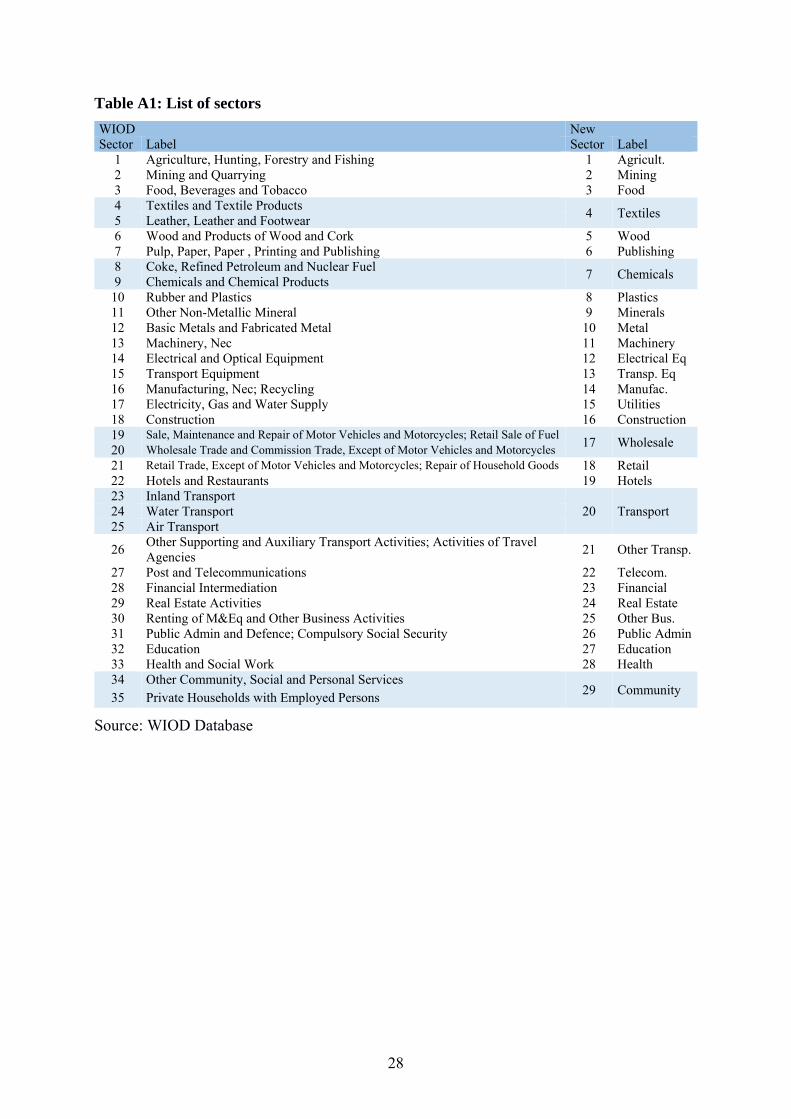
associated with zero output and consumption we aggregate the data to 29 industries according

to table 1 in the appendix. The countries include all current members of the European Union,

except for Croatia which has not been a part of the Union in 2011, as well as the US and all

major trading partners of the EU and the US. The complete list is provided in table 2 in the

appendix. We use the resulting input-output table to derive the consumption and intermediate

good shares ( and ), the share of value added ( ) and the bilateral industry trade

shares ( ). Appendix A1 explains this derivation and details how we handle inventory

changes and zeros in bilateral trade flows.

In line with the previous literature we choose a value of 0.75for the share of goods in

consumption.5 To split value added between labor and land, we borrow from Davis and Ortalo-

Magné (2011), who calculate the income shares of land and structures for different US sectors.

In particular we set the share of land in value added at 32%, 15%, 9%, and 21% in agricultural,

manufacturing, construction and service sectors, respectively.

For data on the labor force we rely on the WIOD Socio Economic Accounts (SEA). We use the

numbers for ‘people engaged’, which include self-employed and family-workers, for the year

4 There is also zero production in Cyprus, Luxembourg, Latvia and Malta in ‘coke, refined petroleum and nuclear fuel’ and for several countries in the sector ‘private households with employed persons’ and zero consumption in Latvia and Cyprus in ‘water transport’, in Luxembourg in ‘air transport’ and, again in several countries in the sector ‘private households with employed persons’. 5 This accords with Redding (2014). A slightly lower value of 73.6% is reported by Statistisches Bundesamt (2011) for Germany.

13

2011 which are consistent with the data above.6 Since, there is no value for ROW we use the

International Labor Associations’ estimate of the worldwide work force of 3 billion people and

subtract the work force of all other countries in our model.

4 The liberalization of transatlantic trade

4.1 Pure Trade Effects

In response to the uncertainties concerning the outcome of the trade negotiations and the

inherent difficulties to derive tariff equivalents for non-tariff barriers, we consider a range of

conceivable reductions of non-tariff barriers between the EU and the US. We keep this range

within the lines hypothesized in previous studies so that the most ambitious scenario that we

consider involves a non-tariff barrier reduction by 25%.

Real income changes - pure trade. Figure 1 reports our findings for the change in real incomes,

≡ ⁄ from eq. (25) for the pure trade scenario, 1 (no labor mobility in

Europe). As can be seen, there are two very strong winners in Europe, Ireland and Luxembourg.

In the most ambitious scenario of a trade barrier reduction of 25%, Ireland would reap a real

income gain of more than 13% and Luxembourg of more than 4%. Great Britain, the

Netherlands and Belgium are the only other countries that gain (slightly) more than 2%. In the

selection of countries shown, the United States and Germany follow with real income gains at

around 1.7% and 1.5% (table 3 in the appendix provides the full list of results). In the full

sample only Sweden experience similar effects as the United States. For the rest of the countries

the quantitative effects are much milder, even in this most ambitious scenario. Figure 1 also

reveals that there is trade diversion: Taiwan and the ROW-countries experience negative

welfare effects. Trade diversion is similarly strong for Mexico and Canada, as these countries

are very tightly integrated with the United States but would not be involved in transatlantic

trade liberalization.

Figure 2 provides complementary information concerning the initial spending shares on US

goods and services. We have ordered the countries from the strongest losers of transatlantic

trade liberalization (Taiwan, Korea, Russia, Mexico, China and Canada) to the strongest

winners, Great Britain, Luxembourg and Ireland. It becomes apparent that both the strongest

winners and the strongest losers exhibit the closest ex-ante connections with the United States

(except for Russia which has strong ties with the EU): the spending shares on US goods and

6 See Timmer (2012) and Timmer et al. (2007) for details on the work force data.

14

services from Luxembourg and Ireland are in the range of 9% to 10% and the spending shares

of Canada and Mexico are only slightly lower, at around 8%. Figure 2 reveals in addition that

the limited overall welfare results, that we have diagnose, stem from the small share that US

goods have in overall spending in most of the countries. For most countries apart from the

mentioned ones, these shares are well below 2%.

Figure 1: Welfare effects of trade barrier reduction; pure trade regime

Figure 2: Welfare effects and initial spending shares

15

Figure 3 provides a detailed look into the fabrics of the real income changes. As is clear from

eq. (17), real income is composed of nominal income, goods prices and land prices. A

breakdown of the overall welfare change into the changes in goods prices and incomes and land

rents is provided in that figure. The numbers reported are for the most ambitious trade

liberalization scenario. It is interesting to note that the overall welfare effects have very

heterogeneous roots.

Figure 3: The components of welfare changes

For Ireland, Great Britain and the USA, the overall welfare gain is due to a strong increase in

wages which overcompensates rising goods and land prices. The positive real income effects

in most Northern and Western EU countries, such as Luxembourg, the Netherlands, Belgium,

Denmark, Italy, France, and Spain are driven by both wage gains and falling goods prices.

Several Eastern and Southeastern European countries, on the other hand, experience falling

16

wages that are overcompensated by drastic price and land rent reductions. Finally, falling prices

both for goods and for land also buffer the negative effects of trade diversion in third party

countries, resulting in only minimal welfare losses. In the case of India and Australia, who

compensate trade losses by increasing their bilateral ties, falling prices even lead to overall real

income gains despite reduced wages.

Industry effects. We have also looked at the changes in the industry mix (measured by

production values) that is implied by transatlantic trade liberalization. Figure 4 reports the

results on industry mix, again under the assumption of the most ambitious liberalization path.

Germany is representative for many other countries in that there is only little effect on the

industry mix. As can be seen, there are only very small effects, if any, in most of the industries.

The strongest changes occur in electrical equipment and metal which would thrive under

transatlantic trade liberalization whilst telecommunications, transport, other transport activities,

mining and agriculture shrink. Ireland, which would be the overall winner in welfare terms,

experiences strong effects, in some industries, however. Financial, electrical equipment and

chemical products (including pharmaceuticals) would experience a strong boost.

Figure 4: Effects on the industry mix: Germany vs. Ireland

17

The role of land. A key innovation of our analysis in relation to previous studies of transatlantic

trade liberalization is that we integrate land, notably as a consumption good, but also as a

production factor. This has important consequences, as can already be seen from the following

theoretical thought experiment. Suppose that land is only used for housing purposes, but not as

an input in production ( 0 . It then follows immediately from (14) and (17) that ̂

and from (17) that ⁄ . Ignoring land in consumption ( 1 would thus lead to

an overestimation of the welfare effects of the magnitude 1 / . For plausible values of

the share of land in consumption of 1/4, disregarding land in consumption hence implies an

overestimation of real income effects in the range of 1/3.

Turning to the full model with land used as a consumption good and as an input in production,

our numerical analyses suggest that real income effects of plausible TTIP-scenarios would be

overestimated by about 33% percent (see table 4 in the appendix). These simulations also reveal

that the effects of disregarding land in production are by several magnitudes smaller compared

to omitting land for housing.7

The upshot of this section is that studies which disregard land are prone to overestimate the

static real income effects of transatlantic trade liberalization. This difference explains at the

same time, why we find more limited effects than previous analyses. It should also be pointed

out that, by highlighting the role of land, our analysis also contributes to the more general

discussion of the sensitivity of the new quantitative trade models to auxiliary assumptions (see

Costinot and Rodriguez-Claré 2014, section 5).

4.2 The local perspective: Germany

Awareness of the local labor market consequences of shifts in the global economy has been

growing recently both in public and in academics (see e.g. Autor et al. 2013; Dauth et al. 2014;

Moretti 2010). Public concern over transatlantic trade liberalization is similarly strong, in

particular in Europe. It is therefore important to explore how local labor markets within

countries are affected by a transatlantic deal. We take Germany as a case in point and trace the

effects of trade liberalization down to the local level.

Data. For this purpose we use value added data from national accounts which is available on

the regional level from the German federal and state statistical offices (“Regionaldatenbank der

Statistischen Ämter des Bundes und der Länder”). This data is available for all 402 regions

7 The effects become more pronounced, however, in the regime with population mobility, but still small compared to the effects derived omitting land in consumption.

18

(“Kreise”) disaggregated into 6 groups of NACE/ISIC industries which match directly with

WIOD industries as can be seen in table 4 in the appendix. We label these sectors “Agriculture”,

“Manufacturing”, which includes mining and raw materials, “Construction”, “Trade”, which

includes transportation and tourism, “Financial” and “Government”, which includes health and

education. Assuming that the German input output structure holds for all German regions we

can use our data to rewrite the World Input Output table in terms of our new 6 sectors and

including 402 German regions instead of the country as a whole. This method is explained in

detail in section A2 in the appendix.

Descriptive evidence. The initial heterogeneity in the industry mix across locations is portrayed

in Fig. A1 in the appendix. Regions in the Northwest and in the Northeast of Germany have the

strongest focus on agriculture, though no region produces much more than 10% of its value

added in this sector. Manufacturing, in contrast, is of bigger importance for locations in the

South of Germany and especially for regions in which 3 major car manufacturers (VW, BMW

and Mercedes) are active. In these locations it can be responsible for more than 80% of value

added. The trade sector, which includes transportation, is most important for those regions that

are close to the two major German airports (Frankfurt and Munich) or have large ports, like

Hamburg.8 In and around Frankfurt where several important German banks, the largest German

stock market and the German central bank are located, the financial sector plays a crucial role

being responsible for up to 50% of total value added in these regions. The share of government

tasks, including health and education, in value added is strongest in regions that consist of only

one large city, and, in general, in the Northeast of Germany.

We can also look at how important regions are for Germany as a whole. Fig. A2 in the appendix

gives the share of a region’s value added in a specific industry relative to Germany’s value

added in this industry. The largest producers in the agricultural sector are found in the

Northwestern regions. All other sectors are, with some exceptions, dominated by the highly

populated regions Berlin, Hamburg, Munich, “Region Hannover”, and Cologne (all above one

million inhabitants).

Transatlantic trade liberalization. We begin by calculating the effects of a 25% barrier

reduction between the US and all EU members without population mobility in order to show

the heterogeneity of expected real income changes. The initial spending shares on US goods

and the real income effects from the policy experiment on regions are shown in Figure 5. It is

8 The bright outlier in the north west of Germany is „Landkreis Leer“, which has the second largest concentration of shipping companies after Hamburg.

19

clear to see, that the initial share of a countries total spending on US goods (both final and

intermediate) is again a very good indicator for its real income changes due to the barrier

reduction. A key finding of our calculations is that despite their heterogeneity all regions win.

This is remarkable, because our model, in principle, allows for negative welfare effects through

terms of trade movements which work through wage adjustments across locations. The fear that

TTIP might benefit only the already rich German locations at the cost of the poor ones is not

supported by our analysis. Yet even in our ambitious scenario the potential gains are limited to

between 1.1 and 1.8 percent of real income (figure A3 in the appendix provides a disaggregation

of the real income effects).

Figure 5: Initial US Spending Shares and Real Income Changes

We show more detailed results for the case with population mobility among German regions

(i.e. only in Germany not between other EU members) in Figure 6 below. Due to the low real

income effects observed under population immobility the incentive to move is limited. The

forecasted effects on population are consequently only in the range of -0.46% to 0.67%, despite

our assumption of perfect mobility. The fear that individual German regions could experience

strong population losses due to a restructuring thus also seems unwarranted.

Wage gains are strongest in the South and West, as well as in the car manufacturing centers.

Price drops are strongest in the vicinity of large cities and in regions that specialize in the

financial or trade sector. However, effects for both prices and wages are very low, and

heterogeneity even more so. Rents increase everywhere, but more in the south and west where

population increases and thus drives demand for land.

20

Figure 6: Detailed effects of 25% barrier reduction with population mobility

4.3 Population mobility in Europe

Figure 7 portrays our findings under the assumption of full labor mobility in the EU. It should

be noted that our model captures only one dispersion force, scarce land, and hence land prices.

Clearly, there are further forces which reduce labor mobility in Europe, in particular

heterogeneous location preferences and a plethora of mobility costs. The results in this section

should therefore be seen as an extreme scenario, just as the no mobility case (depicted in figure

1) goes to the other extreme. The establishment of a spatial equilibrium in the mentioned

extreme case would level all income gains at just below 1.5% in all EU members. Ireland and

Luxembourg would experience a strong inflow of labor followed, with an already much weaker

inflow, by Great Britain, the Netherlands, Belgium, and Sweden. This inflow immensely

reduces wages in these countries, but thereby also lowers production costs and consequently

leads to much lower price increases as compared to the no-mobility case in figure 1. A close

21

inspection of figure 7 reveals that the bulk of the adjustment to the spatial equilibrium within

the European Union takes place through the adjustment of land prices.

Figure 7: Welfare effects in European countries, with labor mobility

4.4 TTIP versus multilateral trade liberalization

An important concern regarding TTIP is that it may undermine the global trading system

(Bagwell et al. 2014; Bhagwati et al. 2014; Panagariya 2013). Our analysis has in fact identified

countries that lose due to trade diversion. An alternative to regional engagements would be to

bring in more effort into the trade talks at the multilateral level, which are currently stalling.

What level of multilateral trade liberalization would have to be achieved in order to match the

real income effects that the European Union and the United States derive from a transatlantic

22

deal? Redoing our calculations for a multilateral trade barrier reduction we find that the answer

differs considerably between the two locations9. A multilateral reduction of trade barriers in the

range of 4% to 5% would be enough for Europe10 to achieve the same welfare gains as in our

most ambitious TTIP scenario. For the US, however, this would require a decrease in

multilateral barriers of 11% to 12%. This level of reductions seems out of reach for multilateral

negotiations that generally focus on tariffs alone. Consequently, the US appears to gain more

from TTIP in comparison to a multilateral agreement, while the same does not necessarily hold

true for the EU. This finding points to the importance of the Bhagwati’s (1994) prediction that

a ‘hegemonic power’ is likely to gain more by bargaining sequentially than simultaneously.

Hence, TTIP might indeed harm the multilateral trading system by diverting the political energy

of one of its key players, the US, away from WTO negotiations.

4.5 Discussion: How deep … ?

Both our model and our empirical strategy differ from earlier studies of the transatlantic trade

partnership. This section briefly puts our results in perspective to previous research.

The difficulties in the ongoing negotiating process between the EU and the US make it

impossible to know how ‘deep’ a final trade agreement is going to be and how the various

sectors will be affected. However, even if we knew the final outcome (e.g. the harmonization

of standards in the car industry or agreements on the testing of pharmaceutical or medical

products), there is no simple way to translate these (reductions of) barriers into tariff

equivalents. The previous literature has dealt with this issue in two different ways. One line has

followed a ‘bottom-up’ approach and has indeed tried to figure out tariff equivalents. This has

led to widely differing results, however. The table below lists the findings that two of the most

influential studies have obtained, Ecorys (2009) on which the study of Francois et al. (2013)

for the EU commission is based, and Fontagné et al. (2013). The number are confined to the

three broad sectors agriculture, manufacturing and services.

Table 1: Estimated tariff equivalents

Ecorys (2013) US → EU

EU → US

Fontagné et al. (2013) US → EU

EU → US

agriculture 56.8 73.3 48.2 51.3 manufacturing 19.3 23.4 42.8 32.3

services 8.5 8.9 32.0 47.3

9 See table 7 in the appendix for detailed results. 10 In the case without population mobility this value, of course, varies across EU member states. However, as can be seen in table 6 in the appendix it remains in the range of 4% to 5% for most, including Germany.

23

In view of the problems and discrepancies, Felbermayr et al. (2013) go so far to argue that no

consistent and reliable quantification is possible on the sectoral level. Felbermayr et al. (2013;

2014) and Aichele et al. (2014) use an alternative ‘top down approach’ whereby estimates of

the effects of existing trade agreements on bilateral trade volumes in different industries are

used to calibrate the TTIP shock to result in these volume changes. Hence instead of providing

a range of conceivable reductions up to an upper bound, as we do, they pick a particular scenario

for their welfare calculations. This has the advantage that it allows for shocks to vary across

industries which opens a further channel for welfare effects. On the other hand, their predictions

can only be as good as their scenario represents the outcome of the TTIP negotiations, or as

good as TTIP remains an “average” trade agreement.

Turning to the results, our estimated welfare effects are within the range of results reported in

the CGE based studies by Francois (2013) and slightly higher than those reported in Fontagné

(2013), all methodological differences notwithstanding. The one-sector new quantitative trade

study by Felbermayr et al. (2014) reports significantly higher welfare effects than we do. They

find that the EU 28 would achieve a welfare gain of 3.9 % and the United States of 4.9 % while

the welfare loss that they compute for the rest of the world is -0.9%. Aichele et al. (2014) which

draws a Ricardian multi-industry model, also forecasts higher welfare gains than we do, with

2.7% for the US and 2.1% for the EU.

Felbermayr et al. (2013) report that the member states at the EU periphery benefit most. This

corresponds to our finding with respect to Ireland. However, we also find that a country at the

geographic center, Luxembourg, would derive extremely strong benefits. Felbermayr et al.

(2013), on the other hand, find that Spain would derive strong gains in the range of 5.6 % which

is strongly at odds with our findings and which is also hard to understand given the small share

of spending that Spain devotes to US goods and services (cf. figure 2.). There are some further

differences. Whereas trade diversion effects appear to play little role in Fontagné (2013), they

are clearly visible in other studies and, for very good reasons, very prominent for Taiwan,

Korea, Russia, Mexico, China, and Canada in our analysis.

What explains these different results? Clearly, part is due to the fact that the estimates are based

on different models which differ along several choices. Our analysis points to the importance

of land in consumption and production and suggests that a disregard of land may imply an

overestimation of the real income gains in the range of 33%. A second important reason for the

difference in results is due to the fact that different liberalization scenarios are considered.

24

The top down approach pursued by Aichele et al (2014) can easily be related to our analysis

(see table A5 in the appendix). Their estimate of previous trade agreements implies that TTIP

would result in very large barrier reductions for agriculture and car manufacturing (barriers fall

by more than 50% in both), as well as food and textiles (both above 30%) but have much lower

effects in the remaining industries and especially low effects in service industries (0.7% to

7.3%). After matching their industry classification to ours we find the following.11 First, the

high gains of Ireland and Luxembourg are brought down significantly. This is largely due to

the much smaller cut in trade barriers that Aichele et al. (2014) predict for the service industries

from which these two countries derive the main benefits. Second, for Germany the real income

effect is almost identical to our extreme scenario, despite the lower barrier reductions in most

sectors. The main driver of these gains is the huge predicted trade barrier reduction of more

than 50% in the car manufacturing sector, on which Germany relies heavily. Third, the average

long term effects for the EU with population mobility would be a real income gain of 1.15%

and thus lower than for the upper bound estimate of our across the board reduction (1.49%).

Our main result that effects are low except for some industries in some countries, remains intact,

however.

5 Conclusion

This paper is the first to set up a new quantitative spatial trade model and to employ the method

of Dekle et al. (2007) to evaluate the quantitative consequences of the liberalization of

transatlantic trade associated with the envisioned EU-US trade and investment partnership. The

advantage of this approach is that we do not need information on the initial trade cost matrix to

perform our numerical analysis. The trade costs are extremely hard to quantify since the most

important outstanding trade barriers are of non-tariff nature. Previous analyses have obtained

widely differing results for the tariff equivalents of these barriers and hence, are plagued by

considerable uncertainties. Our approach allows us to circumvent this problem since these

parameters are already embedded in the baseline specification. With our method it is easy to

establish the real income effects for a whole range of trade cost reductions.

We provide new perspectives by highlighting the role of land for the estimation of real income

effects, by looking at local labor markets and by addressing the mobility of labor. Our results

have to be seen against the background of three important caveats. First, for Europe we study a

scenario both with no labor mobility and one with labor mobility hindered only by changing

11 We provide detailed information in a supplementary appendix.

25

land prices. Both these scenarios are to be thought of as the extreme limiting cases. Second, our

analysis sheds only light on static gains from trade liberalization but not on the likely follow-

up effects associated with induced capital accumulation and dynamic growth effects. Third, our

approach, like previous attempts, does not embrace welfare effects associated with FDI. Hence,

our results would have to be scaled up. Future research is needed to embed FDI in the new

quantitative trade models to obtain more accurate overall welfare effects for the investment part

of this (and any other) agreement.

References

Aichele, Rahel, Gabriel Felbermayr and Inga Heiland (2014): Going Deep: The Trade and Welfare Effects of TTIP, CESifo Working Paper 5150

Autor, David H., David Dorn, and Gordon H. Hanson (2013). The China Syndrome: Local Labor Market Effects of Import Competition in the United States. American Economic Review 103:6, 2121-2168

Bagwell, Kyle, Chad P. Bown and Robert W. Staiger (2014). Is the WTO Passé? Mimeo.

Bhagwati, Jagdish (1994). Threats to the World Trading System: Income Distribution and the Selfish Hegemon, Journal of International Affairs, Spring 1994

Bhagwati, Jagdish (2013). Dawn of a New System. Finance and Development, 8-13

Bhagwati, Jagdish, Pravin Krishna and Arvind Panagariya (2014). The World Trade System: Trends and Challenges, Paper presented at the Conference on Trade and Flag: The Changing Balance Of Power in the Multilateral Trade System, April 7‐8, 2014, International Institute for Strategic Studies, Bahrain

Caliendo, Lorenzo and Fernando Parro (2014). Estimates of the Trade and Welfare Effects of NAFTA. Review of Economic Studies, forthcoming

Costinot, Arnaud and Andrés Rodriguez-Claré (2014). Trade Theory with Numbers: Quantifying the Consequences of Globalization. Handbook of International Economics Vol 4, 197-261

Dekle, Robert, Jonathan Eaton and Samuel Kortum (2007). Unbalanced Trade. American Economic Review 97:2, 351-355.

Davis, Morris A. and François Ortalo-Magné (2011). Household expenditures, wages, rents. Review of Economic Dynamics 14:2, 248-261.

Dauth, Wolfgang, Sebastian Findeisen and Jens Suedekum (2015). The Rise of the East and the Far East: German Labor Markets and Trade Integration. Journal of the European Economic Association 12:6, 1643-1675

Eaton, Jonathan and Samuel Kortum (2002). Technology, Geography, and Trade. Econometrica 70:5, 1741-1779.

Economist (2014a). Free-trade agreements. A better way to arbitrate, October 11.

Economist (2014b). Charlemagne. Ships that pass in the night, December 13.

Ecorys (2009). Non-Tariff Measures in EU-US Trade and Investment – An Economic Analysis. Report, prepared by K. Berden, J.F. Francois, S. Tamminen, M. Thelle, and P. Wymenga for the European Commission, Reference OJ 2007/S180-219493.

26

Felbermayr, Gabriel, Benedikt Heid, Mario Larch and Erdal Yalcin (2014). Macroeconomic Potentials of Transatlantic Free Trade: A High Resolution Perspective for Europe and the World, CESifo Working Paper 5019.

Felbermayr, Gabriel, Mario Larch, Lisandra Flach, Erdal Yalcin and Sebastian Benz (2013). Dimensionen und Auswirkungen eines Freihandelsabkommens zwischen der EU und den USA. Final Report, Ifo Institute Munich.

Fontagné, Lionel, Julien Gourdon and Sébastien Jean (2013). Transatlantic Trade: Whither Partnership, Which Economic Consequences? CEPII Policy Brief, CEPII, Paris.

Francois, Joseph, Miriam Manchin, Hanna Norberg, Olga Pindyuk, Patrick Tomberger (2013). Reducing Transatlantic Barriers to Trade and Investment: An Economic Assessment. Report TRADE10/A2/A16 for the European Commissions, IIDE and CEPR.

Fujita, Masahisa and Jacques-Francois Thisse (2013). Economics of Agglomeration. Cities, Industrial Location, and Regional Growth. Second Edition. Cambridge University Press.

Hamilton, Daniel and Joseph Quinlan (2014). The Transatlantic Economy 2014. Center for Transat-lantic Relations Johns Hopkins University. Paul H. Nitze School of Advanced International Studies.

Helpman, Elhanan (1998). The size of regions. In: Pines, D., Sadka, E., Zilcha, I. (Eds.), Topics in Public Economics. Theoretical and Empirical Analysis. Cambridge University Press, 33–54.

Helpman, Elhanan and Paul Krugman (1985). Market Structure and Foreign Trade. MIT-Press.

Lawrence Robert Z. (1996). Regionalism, Multilateralism and Deeper Integration. Washington: Brookings Institution.

Michaels, Guy, Ferdinand Rauch and Stephen J. Redding (2011). Technical Note: An Eaton and Kortum (2002) Model of Urbanization and Structural Transformation. Mimeo, Princeton.

Michaels, Guy, Ferdinand Rauch and Stephen J. Redding (2012). Urbanization and Structural Transformation. Quarterly Journal of Economics 127:2, 535-586.

Moretti, Enrico (2010). Local Labor Markets, in: David Card and Orley Ashenfelter (ed.), Handbook of Labor Economics 4b, 1237-1313

Ossa, Ralph (2014): Trade Wars and Trade Talks with Data. American Economic Review 104:12, 4104-4146

Panagariya, Arvind (2013). Challenges to the Multilateral Trading System and Possible Responses. Economics: The Open Access, Open-Assessment E-Journal, 2013-3.

Pflüger, Michael and Takatoshi Tabuchi (2011). The Size of Regions with Land Use for Production. Regional Science and Urban Economics 40: 481-489

Redding, Stephen J. (2014). Goods Trade, Factor Mobility and Welfare. Mimeo, Princeton.

Statistisches Bundesamt (2011). Wirtschaft und Statistik 5/2011.

Timmer, Marcel P, Ton van Moergastel, Edwin Stuivenwold, Gerard Ypma, Mary O’Mahony and Mari Kangasniemi (2007). EU KLEMS Growth and Productivity Accounts: Part I Methodology. Groningen Growth and Development Centre. National Institute of Economic and Social Research.

Timmer, Marcel P. (2012). The World Input-Output Database (WIOD): Contents, Sources and Methods. WIOD Working Paper Number 10.

27

Appendix

Table A1: List of Sectors

Table A2: Country Sample

Table A3: Detailed effects of a 25% trade barrier reduction

Table A4: The significance of land

Table A5: Detailed results of alternative barrier changing scenarios

Table A6: Multilateral Liberalization - no mobility

Table A7: Multilateral Agreements – mobility within the EU

Figure A1: Shares of different industries in the region’s total production

Figure A2: Shares of a regions’ industry production in Germany’s total industry

production

Figure A3: Regional disaggregation, immobile population

App A1: Derivation of trade shares from the WIOD database

App A2: Derivation of regional trade data; table of regional sectors

Material in the Supplementary Appendix – Not for publication

S1: List of symbols

S2: Sector matching for the Aichele et al. (2014) scenario

S3: Detailed regional effects of a 25% trade barrier reduction

28

Table A1: List of sectors

WIOD New Sector Label Sector Label

1 Agriculture, Hunting, Forestry and Fishing 1 Agricult. 2 Mining and Quarrying 2 Mining 3 Food, Beverages and Tobacco 3 Food 4 Textiles and Textile Products

4 Textiles 5 Leather, Leather and Footwear 6 Wood and Products of Wood and Cork 5 Wood 7 Pulp, Paper, Paper , Printing and Publishing 6 Publishing 8 Coke, Refined Petroleum and Nuclear Fuel

7 Chemicals 9 Chemicals and Chemical Products

10 Rubber and Plastics 8 Plastics 11 Other Non-Metallic Mineral 9 Minerals 12 Basic Metals and Fabricated Metal 10 Metal 13 Machinery, Nec 11 Machinery 14 Electrical and Optical Equipment 12 Electrical Eq 15 Transport Equipment 13 Transp. Eq 16 Manufacturing, Nec; Recycling 14 Manufac. 17 Electricity, Gas and Water Supply 15 Utilities 18 Construction 16 Construction 19 Sale, Maintenance and Repair of Motor Vehicles and Motorcycles; Retail Sale of Fuel

17 Wholesale 20 Wholesale Trade and Commission Trade, Except of Motor Vehicles and Motorcycles 21 Retail Trade, Except of Motor Vehicles and Motorcycles; Repair of Household Goods 18 Retail 22 Hotels and Restaurants 19 Hotels 23 Inland Transport

20 Transport 24 Water Transport 25 Air Transport

26 Other Supporting and Auxiliary Transport Activities; Activities of Travel Agencies

21 Other Transp.

27 Post and Telecommunications 22 Telecom. 28 Financial Intermediation 23 Financial 29 Real Estate Activities 24 Real Estate 30 Renting of M&Eq and Other Business Activities 25 Other Bus. 31 Public Admin and Defence; Compulsory Social Security 26 Public Admin32 Education 27 Education 33 Health and Social Work 28 Health 34 Other Community, Social and Personal Services

29 Community 35 Private Households with Employed Persons

Source: WIOD Database

29

Table A2: Country sample

Code  Country     Code  Country     Code  Country AUS  Australia    FRA  France    MLT  Malta 

AUT  Austria    GBR  Great Britain    NLD  Netherlands 

BEL  Belgium    GRC  Greece    POL  Poland 

BGR  Bulgaria    HUN  Hungary    PRT  Portugal 

BRA  Brazil    IDN  Indonesia    ROU  Romania 

CAN  Canada    IND  India    RUS  Russia 

CHN  China    IRL  Ireland    SVK  Slovakia 

CYP  Cyprus    ITA  Italy    SVN  Slovenia 

CZE  Czech Republic    JPN  Japan    SWE  Sweden 

DEU  Germany    KOR  Korea    TUR  Turkey 

DNK  Denmark    LTU  Lithuania    TWN  Taiwan 

ESP  Spain    LUX  Luxemburg    USA  United States of America 

EST  Estonia    LVA  Latvia    ROW  Rest of World 

FIN  Finland    MEX  Mexico   

Source: WIOD Database

30

Table A3: Detailed effects of a 25% trade barrier reduction

 real income  prices  wages  rents 

popula‐tion 

   immobile  mobile  immobile  mobile  immobile  mobile  immobile  mobile  mobile 

AUS  0,43%  0,43% ‐0,52%  ‐0,61% 0,08% 0,00% ‐0,08%  ‐0,16% 0,00%

AUT  1,08%  1,49% ‐0,36%  ‐0,38% 1,07% 1,29% 0,93%  0,13% ‐1,00%

BEL  2,09%  1,49% ‐0,14%  ‐0,33% 2,54% 1,99% 2,50%  3,50% 1,49%

BGR  0,52%  1,49% ‐0,83%  ‐0,74% ‐0,17% 0,38% ‐0,07%  ‐1,49% ‐2,04%

BRA  ‐0,03%  ‐0,03% ‐1,16%  ‐1,24% ‐1,20% ‐1,28% ‐1,17%  ‐1,26% 0,00%

CAN  ‐0,18%  ‐0,18% ‐1,20%  ‐1,28% ‐1,46% ‐1,53% ‐1,32%  ‐1,40% 0,00%

CHN  ‐0,21%  ‐0,21% ‐1,82%  ‐1,90% ‐2,01% ‐2,08% ‐1,98%  ‐2,05% 0,00%

CYP  0,54%  1,49% ‐1,92%  ‐1,78% ‐1,49% ‐0,94% ‐1,14%  ‐2,29% ‐1,84%

CZE  1,21%  1,49% ‐1,22%  ‐1,25% 0,36% 0,51% 0,33%  ‐0,24% ‐0,69%

DEU  1,55%  1,49% 0,04%  ‐0,07% 1,95% 1,80% 1,88%  1,89% 0,15%

DNK  1,60%  1,49% ‐0,20%  ‐0,31% 1,80% 1,63% 1,77%  1,90% 0,30%

ESP  1,13%  1,49% ‐0,24%  ‐0,24% 1,34% 1,52% 1,18%  0,56% ‐0,80%

EST  1,07%  1,49% 0,07%  0,04% 1,46% 1,69% 1,12%  0,18% ‐1,11%

FIN  1,49%  1,49% 0,86%  0,75% 2,88% 2,78% 2,62%  2,51% ‐0,01%

FRA  0,92%  1,49% ‐0,07%  ‐0,03% 1,20% 1,54% 1,10%  0,16% ‐1,27%

GBR  2,33%  1,49% 1,02%  0,86% 4,34% 3,74% 3,64%  5,17% 2,07%

GRC  0,61%  1,49% ‐1,16%  ‐1,04% ‐0,42% 0,09% ‐0,32%  ‐1,45% ‐1,75%

HUN  1,61%  1,49% ‐1,32%  ‐1,44% 0,82% 0,61% 0,48%  0,52% 0,23%

IDN  ‐0,06%  ‐0,06% ‐1,48%  ‐1,57% ‐1,52% ‐1,61% ‐1,49%  ‐1,58% 0,00%

IND  0,30%  0,30% ‐1,62%  ‐1,70% ‐1,30% ‐1,37% ‐1,10%  ‐1,16% 0,00%

IRL  13,61%  1,49% 3,76%  1,02% 16,83% 3,37% 19,40%  52,08% 39,80%

ITA  0,76%  1,49% ‐0,13%  ‐0,08% 0,93% 1,35% 0,78%  ‐0,48% ‐1,67%

JPN  ‐0,05%  ‐0,05% ‐1,63%  ‐1,72% ‐1,70% ‐1,78% ‐1,68%  ‐1,76% 0,00%

KOR  ‐0,26%  ‐0,27% ‐1,63%  ‐1,72% ‐1,87% ‐1,96% ‐1,83%  ‐1,92% 0,00%

LTU  0,27%  1,49% ‐0,86%  ‐0,73% ‐0,49% 0,29% ‐0,60%  ‐2,58% ‐2,78%

LUX  4,19%  1,49% ‐0,45%  ‐1,41% 3,45% ‐0,48% 4,24%  11,93% 10,28%

LVA  0,27%  1,49% ‐1,17%  ‐0,99% ‐0,82% 0,01% ‐0,83%  ‐2,75% ‐2,76%

MEX  ‐0,22%  ‐0,22% ‐1,72%  ‐1,81% ‐2,02% ‐2,11% ‐1,90%  ‐1,99% 0,00%

MLT  1,59%  1,49% 1,35%  1,26% 3,87% 3,73% 3,45%  3,59% 0,26%

NLD  2,16%  1,49% ‐1,31%  ‐1,50% 1,32% 0,68% 1,61%  2,92% 1,85%

POL  1,03%  1,49% ‐0,91%  ‐0,92% 0,48% 0,73% 0,32%  ‐0,51% ‐1,07%

PRT  0,73%  1,49% 0,14%  0,22% 1,26% 1,69% 1,07%  ‐0,04% ‐1,58%

ROU  0,27%  1,49% ‐1,11%  ‐0,97% ‐0,79% ‐0,07% ‐0,83%  ‐2,68% ‐2,65%

RUS  ‐0,25%  ‐0,25% ‐1,71%  ‐1,80% ‐1,88% ‐1,98% ‐1,87%  ‐1,97% 0,00%

SVK  0,34%  1,49% ‐1,28%  ‐1,16% ‐0,82% ‐0,04% ‐0,80%  ‐2,74% ‐2,69%

SVN  0,69%  1,49% ‐1,03%  ‐0,97% ‐0,11% 0,38% ‐0,16%  ‐1,54% ‐1,86%

SWE  1,75%  1,49% 0,13%  ‐0,01% 2,32% 2,01% 2,20%  2,61% 0,68%

TUR  0,04%  0,05% ‐1,10%  ‐1,17% ‐1,17% ‐1,24% ‐1,07%  ‐1,14% 0,00%

TWN  ‐0,54%  ‐0,54% ‐1,97%  ‐2,06% ‐2,40% ‐2,50% ‐2,43%  ‐2,53% 0,00%

USA  1,74%  1,77% 0,61%  0,56% 3,07% 3,06% 3,01%  3,00% 0,00%

RoW  ‐0,13%  ‐0,12% ‐1,38%  ‐1,48% ‐1,62% ‐1,71% ‐1,46%  ‐1,55% 0,00%

31

Table A4: The significance of land

25% barrier reduction ‐ no mobility ‐ change in real income 

 

no land 

land in consumption 

 and production difference to no land

housing only  in consumption 

difference to no land 

additional  housing in  

production effect   

AUS  0,576%  0,432% 33,4% 0,431% 33,5%  0,0002%

AUT  1,438%  1,077% 33,5% 1,076% 33,6%  0,0010%

BEL  2,791%  2,087% 33,7% 2,086% 33,8%  0,0012%

BGR  0,693%  0,518% 33,8% 0,519% 33,5%  ‐0,0010%

BRA  ‐0,038%  ‐0,028% 34,5% ‐0,028% 34,5%  0,0000%

CAN  ‐0,239%  ‐0,180% 32,8% ‐0,180% 33,1%  ‐0,0004%

CHN  ‐0,273%  ‐0,205% 32,9% ‐0,205% 33,1%  ‐0,0004%

CYP  0,722%  0,541% 33,6% 0,541% 33,5%  ‐0,0002%

CZE  1,623%  1,214% 33,7% 1,215% 33,6%  ‐0,0008%

DEU  2,070%  1,551% 33,5% 1,549% 33,7%  0,0020%

DNK  2,141%  1,602% 33,6% 1,601% 33,7%  0,0011%

ESP  1,510%  1,131% 33,5% 1,131% 33,6%  0,0005%

EST  1,427%  1,071% 33,2% 1,068% 33,6%  0,0032%

FIN  1,983%  1,485% 33,5% 1,483% 33,7%  0,0021%

FRA  1,235%  0,925% 33,6% 0,925% 33,6%  0,0001%

GBR  3,116%  2,331% 33,7% 2,328% 33,8%  0,0029%

GRC  0,820%  0,615% 33,4% 0,615% 33,4%  0,0001%

HUN  2,144%  1,609% 33,2% 1,603% 33,7%  0,0058%

IDN  ‐0,080%  ‐0,060% 32,8% ‐0,060% 33,3%  ‐0,0002%

IND  0,400%  0,299% 33,6% 0,300% 33,4%  ‐0,0005%

IRL  18,426%  13,611% 35,4% 13,524% 36,2%  0,0876%

ITA  1,019%  0,764% 33,3% 0,764% 33,5%  0,0007%

JPN  ‐0,066%  ‐0,049% 33,7% ‐0,050% 33,1%  0,0002%

KOR  ‐0,347%  ‐0,261% 33,1% ‐0,260% 33,4%  ‐0,0007%

LTU  0,364%  0,274% 32,9% 0,273% 33,3%  0,0009%

LUX  5,593%  4,192% 33,4% 4,166% 34,3%  0,0256%

LVA  0,364%  0,273% 33,5% 0,273% 33,3%  ‐0,0004%

MEX  ‐0,286%  ‐0,215% 33,0% ‐0,215% 33,1%  ‐0,0001%

MLT  2,129%  1,592% 33,8% 1,592% 33,7%  ‐0,0005%

NLD  2,896%  2,161% 34,0% 2,164% 33,8%  ‐0,0030%

POL  1,376%  1,031% 33,4% 1,030% 33,5%  0,0007%

PRT  0,972%  0,728% 33,5% 0,728% 33,5%  0,0000%

ROU  0,365%  0,274% 33,2% 0,274% 33,2%  0,0001%

RUS  ‐0,326%  ‐0,246% 32,6% ‐0,245% 33,1%  ‐0,0011%

SVK  0,461%  0,344% 34,1% 0,345% 33,5%  ‐0,0015%

SVN  0,921%  0,689% 33,6% 0,690% 33,5%  ‐0,0002%

SWE  2,340%  1,752% 33,6% 1,750% 33,7%  0,0024%

TUR  0,060%  0,045% 33,5% 0,045% 33,4%  0,0000%

TWN  ‐0,712%  ‐0,536% 32,7% ‐0,535% 33,2%  ‐0,0017%

USA  2,328%  1,740% 33,8% 1,741% 33,7%  ‐0,0011%

RoW  ‐0,170%  ‐0,128% 32,6% ‐0,127% 33,5%  ‐0,0008%

32

Table A5: Detailed effects of a 25% trade barrier reduction, alternative scenarios

  Scenario from Aichele et al. (2014)  Autarky   immobile  immobile   real income  prices  wages  rents  real income prices  wages  rents 

AUS  0,36%  ‐0,87%  ‐0,43%  ‐0,18%  ‐6,79%  6,48%  ‐3,09%  ‐2,92% 

AUT  0,63%  ‐0,46%  0,42%  0,13%  ‐22,61%  41,14%  0,30%  0,23% 

BEL  1,28%  ‐0,47%  1,18%  1,19%  ‐30,45%  66,48%  2,59%  2,55% 

BGR  1,02%  ‐0,83%  0,51%  0,82%  ‐18,84%  30,23%  ‐1,17%  ‐2,48% 

BRA  ‐0,04%  ‐0,86%  ‐0,88%  ‐1,01%  ‐3,34%  4,70%  0,17%  ‐0,39% 

CAN  0,00%  ‐0,50%  ‐0,49%  ‐0,57%  ‐10,44%  13,72%  ‐1,84%  ‐1,81% 

CHN  ‐0,16%  ‐1,31%  ‐1,45%  ‐1,48%  ‐4,30%  8,70%  2,51%  2,52% 

CYP  1,13%  1,04%  2,83%  3,75%  ‐18,06%  28,84%  ‐0,88%  ‐2,59% 

CZE  0,68%  ‐1,03%  ‐0,05%  ‐0,44%  ‐20,52%  39,99%  2,94%  3,65% 

DEU  1,42%  ‐0,65%  1,18%  0,92%  ‐11,83%  21,50%  2,57%  3,34% 

DNK  0,79%  ‐0,01%  1,01%  0,79%  ‐17,83%  34,46%  3,49%  3,51% 

ESP  1,21%  ‐0,92%  0,73%  0,58%  ‐9,03%  13,10%  ‐0,26%  ‐0,51% 

EST  0,77%  ‐0,04%  1,03%  0,44%  ‐19,89%  37,75%  2,58%  2,10% 

FIN  0,76%  0,41%  1,49%  1,11%  ‐10,66%  19,57%  2,82%  3,18% 

FRA  1,00%  ‐0,76%  0,62%  0,36%  ‐9,89%  14,30%  ‐0,46%  ‐0,73% 

GBR  1,57%  0,05%  2,10%  2,43%  ‐11,71%  17,25%  ‐0,61%  ‐0,97% 

GRC  0,70%  ‐1,24%  ‐0,38%  ‐0,29%  ‐10,16%  12,98%  ‐1,73%  ‐3,38% 

HUN  0,53%  ‐1,26%  ‐0,33%  ‐1,31%  ‐25,58%  52,36%  2,82%  2,51% 

IDN  ‐0,05%  ‐1,01%  ‐1,02%  ‐1,16%  ‐6,97%  7,57%  ‐2,38%  ‐2,03% 

IND  0,20%  ‐1,22%  ‐0,92%  ‐1,18%  ‐4,96%  5,25%  ‐1,45%  ‐2,44% 

IRL  4,40%  0,65%  4,91%  5,19%  ‐22,19%  48,15%  5,82%  6,88% 

ITA  0,92%  ‐0,74%  0,57%  0,09%  ‐7,78%  13,52%  1,90%  1,88% 

JPN  ‐0,03%  ‐1,13%  ‐1,16%  ‐1,15%  ‐2,69%  4,69%  0,93%  1,05% 

KOR  ‐0,19%  ‐1,12%  ‐1,30%  ‐1,28%  ‐8,74%  24,49%  10,03%  10,99%

LTU  0,52%  ‐1,93%  ‐1,12%  ‐1,87%  ‐13,55%  23,68%  2,17%  0,53% 

LUX  1,20%  ‐1,84%  ‐0,14%  ‐0,39%  ‐76,77%  859,43%  37,53%  34,91%

LVA  0,42%  ‐0,66%  ‐0,10%  ‐0,08%  ‐21,54%  36,28%  ‐1,14%  ‐2,38% 

MEX  ‐0,09%  ‐1,00%  ‐1,09%  ‐1,27%  ‐10,72%  13,12%  ‐2,76%  ‐2,74% 

MLT  1,61%  0,01%  2,37%  2,14%  ‐50,00%  156,52%  2,19%  0,22% 

NLD  1,84%  0,31%  2,24%  3,49%  ‐20,89%  43,55%  4,98%  5,24% 

POL  0,51%  ‐1,55%  ‐0,73%  ‐1,44%  ‐15,47%  27,09%  1,57%  1,61% 

PRT  1,11%  ‐1,33%  0,24%  ‐0,25%  ‐13,34%  18,17%  ‐2,28%  ‐2,74% 

ROU  0,35%  ‐2,35%  ‐1,80%  ‐2,95%  ‐10,35%  12,65%  ‐2,45%  ‐3,36% 

RUS  0,03%  ‐0,58%  ‐0,49%  ‐0,55%  ‐11,39%  10,95%  ‐5,63%  ‐5,31% 

SVK  0,12%  ‐1,24%  ‐0,97%  ‐1,40%  ‐21,21%  41,44%  2,94%  2,90% 

SVN  0,49%  ‐1,02%  ‐0,32%  ‐0,61%  ‐24,74%  47,02%  0,62%  0,72% 

SWE  0,96%  ‐0,24%  1,07%  0,51%  ‐12,14%  22,13%  2,70%  3,03% 

TUR  0,02%  ‐0,96%  ‐1,01%  ‐1,08%  ‐12,17%  16,07%  ‐2,29%  ‐2,68% 

TWN  ‐0,45%  ‐1,52%  ‐1,87%  ‐2,07%  ‐12,50%  36,71%  14,31%  14,85%

USA  1,31%  0,31%  2,10%  2,33%  ‐4,16%  5,20%  ‐0,48%  ‐1,06% 

RoW  ‐0,04%  ‐0,73%  ‐0,77%  ‐0,95%  ‐11,23%  14,31%  ‐2,57%  ‐2,08% 

33

Table A6: Multilateral Liberalization - no mobility

Real income effects for different level of multilateral trade barrier reductions Reduction:  1%  2%  3%  4% 5% 6% 7% 8%  9% 10%

AUS  0,20%  0,42%  0,64%  0,88% 1,12% 1,38% 1,66% 1,95%  2,25% 2,58%

AUT  0,41%  0,84%  1,28%  1,74% 2,22% 2,71% 3,23% 3,77%  4,33% 4,91%

BEL  0,56%  1,14%  1,75%  2,37% 3,02% 3,68% 4,38% 5,09%  5,84% 6,61%

BGR  0,40%  0,83%  1,28%  1,74% 2,24% 2,75% 3,30% 3,87%  4,47% 5,10%

BRA  0,10%  0,22%  0,34%  0,46% 0,60% 0,74% 0,89% 1,06%  1,23% 1,42%

CAN  0,27%  0,56%  0,86%  1,18% 1,51% 1,86% 2,22% 2,61%  3,01% 3,42%

CHN  0,15%  0,30%  0,46%  0,64% 0,82% 1,01% 1,22% 1,44%  1,68% 1,93%

CYP  0,26%  0,53%  0,82%  1,11% 1,42% 1,74% 2,08% 2,42%  2,79% 3,16%

CZE  0,56%  1,14%  1,75%  2,38% 3,04% 3,73% 4,44% 5,18%  5,96% 6,77%

DEU  0,30%  0,62%  0,95%  1,29% 1,65% 2,02% 2,41% 2,81%  3,23% 3,67%

DNK  0,37%  0,75%  1,15%  1,55% 1,97% 2,41% 2,86% 3,33%  3,82% 4,32%

ESP  0,21%  0,43%  0,66%  0,90% 1,15% 1,41% 1,68% 1,97%  2,26% 2,57%

EST  0,43%  0,88%  1,34%  1,82% 2,31% 2,82% 3,34% 3,88%  4,44% 5,02%

FIN  0,30%  0,62%  0,95%  1,30% 1,66% 2,04% 2,44% 2,86%  3,29% 3,74%

FRA  0,20%  0,41%  0,63%  0,86% 1,10% 1,34% 1,60% 1,87%  2,15% 2,44%

GBR  0,26%  0,53%  0,81%  1,11% 1,41% 1,74% 2,08% 2,43%  2,81% 3,20%

GRC  0,20%  0,41%  0,63%  0,86% 1,11% 1,36% 1,62% 1,90%  2,18% 2,48%

HUN  0,63%  1,28%  1,96%  2,67% 3,40% 4,16% 4,94% 5,76%  6,61% 7,49%

IDN  0,19%  0,39%  0,60%  0,81% 1,04% 1,28% 1,53% 1,80%  2,07% 2,37%

IND  0,15%  0,30%  0,46%  0,63% 0,81% 1,00% 1,20% 1,41%  1,64% 1,88%

IRL  0,92%  1,88%  2,88%  3,92% 4,99% 6,10% 7,26% 8,46%  9,70% 10,99%

ITA  0,20%  0,40%  0,61%  0,84% 1,07% 1,32% 1,58% 1,85%  2,13% 2,43%

JPN  0,10%  0,20%  0,31%  0,43% 0,55% 0,68% 0,81% 0,95%  1,10% 1,26%

KOR  0,34%  0,69%  1,07%  1,46% 1,87% 2,30% 2,75% 3,23%  3,73% 4,25%

LTU  0,36%  0,73%  1,12%  1,53% 1,96% 2,41% 2,87% 3,36%  3,87% 4,40%

LUX  1,36%  2,78%  4,24%  5,75% 7,32% 8,95% 10,63% 12,37%  14,17% 16,03%

LVA  0,34%  0,70%  1,07%  1,46% 1,85% 2,27% 2,69% 3,14%  3,60% 4,08%

MEX  0,25%  0,52%  0,79%  1,08% 1,37% 1,67% 1,99% 2,32%  2,66% 3,00%

MLT  0,59%  1,19%  1,83%  2,49% 3,17% 3,89% 4,63% 5,40%  6,21% 7,04%

NLD  0,46%  0,94%  1,44%  1,96% 2,50% 3,06% 3,64% 4,25%  4,88% 5,54%

POL  0,34%  0,70%  1,07%  1,45% 1,86% 2,28% 2,72% 3,18%  3,66% 4,16%

PRT  0,25%  0,50%  0,77%  1,06% 1,35% 1,66% 1,98% 2,32%  2,67% 3,04%

ROU  0,27%  0,56%  0,86%  1,17% 1,50% 1,84% 2,19% 2,56%  2,95% 3,36%

RUS  0,25%  0,51%  0,78%  1,06% 1,36% 1,66% 1,99% 2,32%  2,67% 3,04%

SVK  0,47%  0,96%  1,48%  2,01% 2,56% 3,13% 3,72% 4,34%  4,98% 5,64%

SVN  0,40%  0,82%  1,26%  1,71% 2,18% 2,66% 3,16% 3,68%  4,22% 4,79%

SWE  0,35%  0,72%  1,10%  1,49% 1,91% 2,34% 2,78% 3,25%  3,73% 4,24%

TUR  0,21%  0,43%  0,67%  0,91% 1,16% 1,43% 1,71% 2,00%  2,31% 2,64%

TWN  0,56%  1,14%  1,74%  2,37% 3,02% 3,69% 4,38% 5,09%  5,83% 6,58%

USA  0,11%  0,23%  0,36%  0,49% 0,64% 0,79% 0,95% 1,12%  1,30% 1,50%

RoW  0,27%  0,55%  0,85%  1,16% 1,48% 1,82% 2,17% 2,53%  2,91% 3,31%

34

Table A7: Multilateral Liberalization – mobility within the EU

Real income effects for different level of multilateral trade barrier reductions  Reduction:  1%  2%  3%  4% 5% 6% 7% 8%  9% 10%

AUS  0,20%  0,42%  0,64%  0,88% 1,12% 1,38% 1,66% 1,95%  2,25% 2,58%

AUT  0,31%  0,63%  0,97%  1,32% 1,69% 2,07% 2,47% 2,88%  3,31% 3,76%

BEL  0,31%  0,63%  0,97%  1,32% 1,69% 2,07% 2,47% 2,88%  3,31% 3,76%

BGR  0,31%  0,63%  0,97%  1,32% 1,69% 2,07% 2,47% 2,88%  3,31% 3,76%

BRA  0,10%  0,22%  0,34%  0,46% 0,60% 0,74% 0,89% 1,06%  1,23% 1,42%

CAN  0,27%  0,56%  0,86%  1,18% 1,51% 1,86% 2,22% 2,61%  3,01% 3,42%

CHN  0,15%  0,30%  0,46%  0,64% 0,82% 1,02% 1,22% 1,44%  1,68% 1,93%

CYP  0,31%  0,63%  0,97%  1,32% 1,69% 2,07% 2,47% 2,88%  3,31% 3,76%

CZE  0,31%  0,63%  0,97%  1,32% 1,69% 2,07% 2,47% 2,88%  3,31% 3,76%

DEU  0,31%  0,63%  0,97%  1,32% 1,69% 2,07% 2,47% 2,88%  3,31% 3,76%

DNK  0,31%  0,63%  0,97%  1,32% 1,69% 2,07% 2,47% 2,88%  3,31% 3,76%

ESP  0,31%  0,63%  0,97%  1,32% 1,69% 2,07% 2,47% 2,88%  3,31% 3,76%

EST  0,31%  0,63%  0,97%  1,32% 1,69% 2,07% 2,47% 2,88%  3,31% 3,76%

FIN  0,31%  0,63%  0,97%  1,32% 1,69% 2,07% 2,47% 2,88%  3,31% 3,76%

FRA  0,31%  0,63%  0,97%  1,32% 1,69% 2,07% 2,47% 2,88%  3,31% 3,76%

GBR  0,31%  0,63%  0,97%  1,32% 1,69% 2,07% 2,47% 2,88%  3,31% 3,76%

GRC  0,31%  0,63%  0,97%  1,32% 1,69% 2,07% 2,47% 2,88%  3,31% 3,76%

HUN  0,31%  0,63%  0,97%  1,32% 1,69% 2,07% 2,47% 2,88%  3,31% 3,76%

IDN  0,19%  0,39%  0,60%  0,81% 1,04% 1,28% 1,53% 1,80%  2,07% 2,37%

IND  0,15%  0,30%  0,46%  0,63% 0,81% 1,00% 1,20% 1,42%  1,64% 1,88%

IRL  0,31%  0,63%  0,97%  1,32% 1,69% 2,07% 2,47% 2,88%  3,31% 3,76%

ITA  0,31%  0,63%  0,97%  1,32% 1,69% 2,07% 2,47% 2,88%  3,31% 3,76%

JPN  0,10%  0,20%  0,31%  0,43% 0,55% 0,68% 0,81% 0,95%  1,10% 1,26%

KOR  0,34%  0,70%  1,07%  1,46% 1,87% 2,30% 2,75% 3,23%  3,73% 4,25%

LTU  0,31%  0,63%  0,97%  1,32% 1,69% 2,07% 2,47% 2,88%  3,31% 3,76%

LUX  0,31%  0,63%  0,97%  1,32% 1,69% 2,07% 2,47% 2,88%  3,31% 3,76%

LVA  0,31%  0,63%  0,97%  1,32% 1,69% 2,07% 2,47% 2,88%  3,31% 3,76%

MEX  0,25%  0,52%  0,79%  1,08% 1,37% 1,67% 1,99% 2,32%  2,65% 3,00%

MLT  0,31%  0,63%  0,97%  1,32% 1,69% 2,07% 2,47% 2,88%  3,31% 3,76%

NLD  0,31%  0,63%  0,97%  1,32% 1,69% 2,07% 2,47% 2,88%  3,31% 3,76%

POL  0,31%  0,63%  0,97%  1,32% 1,69% 2,07% 2,47% 2,88%  3,31% 3,76%

PRT  0,31%  0,63%  0,97%  1,32% 1,69% 2,07% 2,47% 2,88%  3,31% 3,76%

ROU  0,31%  0,63%  0,97%  1,32% 1,69% 2,07% 2,47% 2,88%  3,31% 3,76%

RUS  0,25%  0,51%  0,78%  1,06% 1,36% 1,66% 1,98% 2,32%  2,67% 3,04%

SVK  0,31%  0,63%  0,97%  1,32% 1,69% 2,07% 2,47% 2,88%  3,31% 3,76%

SVN  0,31%  0,63%  0,97%  1,32% 1,69% 2,07% 2,47% 2,88%  3,31% 3,76%

SWE  0,31%  0,63%  0,97%  1,32% 1,69% 2,07% 2,47% 2,88%  3,31% 3,76%

TUR  0,21%  0,43%  0,67%  0,91% 1,16% 1,43% 1,71% 2,01%  2,31% 2,64%

TWN  0,56%  1,14%  1,74%  2,37% 3,02% 3,69% 4,38% 5,09%  5,83% 6,58%

USA  0,11%  0,23%  0,36%  0,50% 0,64% 0,79% 0,96% 1,13%  1,31% 1,50%

RoW  0,27%  0,56%  0,85%  1,16% 1,49% 1,83% 2,18% 2,54%  2,93% 3,32%

35

Figure A1: Shares of different industries in the region’s total production

Figure A2: Shares of a regions’ industry production in Germany’s total industry

production

36

Figure A3: Regional disaggregation, immobile population

37

App A1: Derivation of trade shares from the WIOD database

For each combination of countries and sectors the WIOD contains an entry , of flows from

industry in country to industry in country , including within country flows , .

Moreover, it also provides values for flows from industry in country to country that end

up as final consumption by households , , final consumption by non-profit organizations

, , government spending , , investments , and inventory changes , .

Of course, inventory changes can be negative and sometimes they are significantly large. If we

were to calculate final demand by simply summing over consumption, investment, government

spending and inventory changes we would end up with a negative final demand in some

instances. Hence, to reconcile the real world data with our static model that has no room for

inventories we follow Costinot and Rodriguez-Claré (2014) and split the vector of inventory

changes into a vector with all positive changes , and one with all negative changes

, and treat them differently. Positive inventory changes are directly included in the final

demand in the same way that final consumption, government spending and investments are, i.e.

we treat the build up of inventory as if it were consumed in the current period. Formally final

demand in country for goods from industry in country , , , is defined as the sum

, , , , , , .

On the other hand, negative inventory changes are treated as if they were produced (and

consumed) in the current period. To do this, we can not simply increase our output vector by

the respective (absolute) value of inventory changes because the production of the inventory in

the last period also required intermediates and, thus, had a larger overall effect. To see how to

calculate the necessary changes consider an example with countries and sectors in matrix

notation, where is the original total output vector (of size ∗ 1), the matrix of input

coefficients (of size ∗ ∗ ), the final demand vector (of size ∗ 1) including

positive inventory changes and the vector of negative inventory changes (of size ∗

1). Then the total output can be calculated as the sum of intermediate flows, final demand, and

inventory changes as . We want to calculate the new level for which

the final demand vector is unchanged but inventory changes are set to 0, i.e. the total output

if the negative inventory changes had been produced in the current period. Rearranging terms

we get F where is the unit matrix. We then obtain the new input ouput

matrix by combining intermediate good flows and the unchanged final demand vector

.

38

This final input-output table allows us derive to important parameters of the model. Firstly we

can calculate the share that industry k has in the consumption demand of country n by dividing

demand for industry k goods by total demand to get ∑ , /∑ ∑ , . Similarly,

we can derive the share that industry k has in the intermediate demand of industry j in country

n as ∑ , /∑ ∑ , .

Moreover, we can now use the adjusted input output matrix to calculate bilateral trade flows in

each industry by summing over all usages (intermediate use in all industries and final

demand) of in its destination country. Hence, ∑ , , gives the total flows

of industry goods from to . Our bilateral trade flows can be thought of as a set of

matrices, one for each industry, as shown in the figure below.

Figure App-A1-1: Industry specific bilateral trade matrix

When looking at the data, several of these bilateral trade flows will be equal to 0 due to the high

level of sectoral and geographical disaggregation. However, while trade between any two

countries in any industry can become arbitrarily small in the Eaton-Kortum model, it can only

become 0 if trade costs between those two countries were infinitely high. However, in this case

it could no longer hold true that direct trade between those countries would be cheaper than

trade via some partner country (with non-infinite trade costs). To avoid these problems, we set

all zero trade flows equal to a value of 1 US Dollar. Note that after our industry aggregation

process each country produces output in each industry. Since this output will be in the millions,

setting some values to 1 Dollar has no real influence on the other countries' trade shares, which

will be used in our final calculations.

Given this data, we can sum over all exporters to get country 's total spending in industry ,

i.e. ∑ . Summing over the spending in each individual industry gives country 's

total spending as ∑ .

39

Also, summing over all Importers, we can calculate country 's total production in industry ,

i.e. firm revenue in industry , as ∑ . Total production or revenue in country is,

hence, given by ∑ .

Finally, we can also derive the share that country has in country 's spending in industry ,

, by dividing industry flows from to , , by country 's total industry spending .

Again, these shares can be represented by bilateral trade share matrices as shown in the figure

below.

Figure App-A1-2: Industry specific bilateral trade share matrix

40

App A2: Derivation of Regional Trade Data; Table of Regional Sectors

In order to include the German regions into the calculations we start with value added data from

national accounts which are available on the regional level from the German federal and state

statistical offices (“Regionaldatenbank der statistischen Ämter des Bundes und der Länder”).

This data is available for all 402 regions (“Kreise”) disaggregated into 6 groups of NACE/ISIC

industries which match directly with WIOD industries as can be seen in table 4.

Assuming that Germany’s industry specific shares of value added in production

hold for all regions, we can use the value added data to calculate a regions share in total German

production for each industry.

We incorporate regions into the initial input-output table in three steps. Firstly, we replace all

German rows in the table spreading the intermediate and final demand for German goods across

regions according to their production shares. This means that a region with a high output in a

certain industry will satisfy a larger share of demand from any trading partner than a region

with low output in that particular industry.

Secondly, we replace all German intermediate demand columns by assuming that the German

intermediate demand structure in each industry holds for all regions. Under this assumption we

can use production shares to determine the intermediate demand levels of each region-industry

from each trading partner. Hence, a region with a high output in, say, agriculture will have a

higher demand for the typical intermediate goods of this sector than a region with low output

in agriculture. Moreover, this region will also feature a higher trade level with whoever is the

principal supplier of such intermediates.

Finally, we need to replace the German final demand column by splitting demand across regions.

To do so, notice that the value of goods consumption is equal to times a region’s total

expenditure given by eq. (14). Thus, a region’s share of total German demand is ∑∈

∑

∑ ∑∈

, where the denominator sums across all German regions. Both the

nominator and denominator of the RHS consist simply of the sum of value added and trade

deficits. We assume that the latter are spread across regions according to total income12 and

consequentially, the above expenditure shares can be calculated using only our value added

data as ∑∈

∑

∑ ∑∈

.

12 Though not in the model, the implicit underlying assumption to justify this decision is that of a constant saving rate across German regions.

41

Table App-A2-1: Regional sectors

WIOD Sector  Description Regional Sector 

NACE ISIC  Regional Label

1 Agriculture, Hunting, Forestry and Fishing 1 A Agricultural

2 Mining and Quarrying

2 B-E Manufacturing

3 Food, Beverages and Tobacco

4 Textiles an Textile Products 5 Leather, Leather and Footwear

6 Wood and Products of Wood and Cork

7 Pulp, Paper, Paper , Printing and Publishing 8 Coke, Refined Petroleum and Nuclear Fuel 9 Chemicals and Chemical Products

10 Rubber and Plastics

11 Other Non-Metallic Mineral

12 Basic Metals and Fabricated Metal

13 Machinery, Nec

14 Electrical and Optical Equipment

15 Transport Equipment

16 Manufacturing, Nec; Recycling

17 Electricity, Gas and Water Supply

18 Construction 3 F Construction

19 Sale, Maintenance and Repair of Motor Vehicles and Motorcycles; Retail Sale of Fuel

4 G-J Trade

20 Wholesale Trade and Commission Trade, Except of Motor Vehicles and Motorcycles

21

Retail Trade, Except of Motor Vehicles and Motorcycles; Repair of Household Goods

22 Hotels and Restaurants 23 Inland Transport 24 Water Transport 25 Air Transport

26

Other Supporting and Auxiliary Transport Activities; Activities of Travel Agencies

27 Post and Telecommunications

28 Financial Intermediation 5 K-N Financial 29 Real Estate Activities

30 Renting of M&Eq and Other Business Activities

31 Public Admin and Defence; Compulsory Social Security

6 O-T Government 32 Education

33 Health and Social Work 34 Other Community, Social and Personal Services 35 Private Households with Employed Persons

42

Supplementary Web Appendix - Not for publication

for: How Deep is Your Love? A Quantitative Spatial Analysis of the

Transatlantic Trade Partnership

By Oliver Krebs and Michael Pflüger

S1: List of symbols

S2: Sector matching for the Aichele et al. (2014) scenario

S3: Detailed regional effects of a 25% trade barrier reduction

43

S1: List of symbols

share of housing in consumption cost share of labor goods and services consumption index in n consumption index of industry k goods in n cost of an input bundle in industry k in country n trade deficit of country n iceberg trade costs for shipping an industry k good from country i to n share of industry k in consumption of individuals from n

share of industry k in intermediate demand of firms from industry j and country n

cost share of land

country and industry specific Frechet distribution function for productivity draws

calculatory constant housing stock in n private housing consumption index for locations/countries index for industries/sectors index for industries/sectors number of sectors number of workers in n worker endowment of m share of workers of country group m living in location n index for country group number of locations/countries country group = set of locations/countries index for locations/countries index for varieties price index for consumption in country n price index for industry k goods in country n

price for variety of industry k offered to consumers in n by a country i firm

share of country i in the expenditure of country n on industry k goods consumption of variety from industry k by an individual from n revenue of industry k in country n rental rates of land in n price index for intermediate demand of an industry k firm in country n elasticity of substitution between varieties in industry k measure of the average productivity in industry k in country n measure of the density of productivities utility of a consumer in n indirect utility = real income of a worker in n total income of one worker in n total labor income of country n wages in n total income of country n productivity draw of a firm in country n and industry k producing variety

44

S2: Sector matching for the Aichele et al (2014) scenario

Aichele et al.  Our Sector Barrier Reduction 

Agri‐Food  Agriculture  0,52519185Mining  Mining  0Food, processed  Food  0,36903795Textiles 

Textiles  0,34027994Leather Wood  Wood  0Paper  Publishing  0,16030053Petroleum   

Chemicals 0

0,10543559Chemicals 

Plastics  0,10543559Mineral products  Minerals  0,07763666Ferrous Metals 

Metal  0,13628883Metals nec Metal products Machinery nec  Machinery  0,11501273Electronics  Electrical Eq  0,22672181Motor vehicles  Transp. Eq  0,50214149Manufactures nec  Manufac.  0,11146342Electricity 

Utilities  0,05672007Gas Water  Construction  Construction  0,05355535

Trade services Wholesale  0,0786294Retail  0,0786294

Recreational services  Hotels  0,03656916Water Transport 

Transport  0,03970704Air transport Transport nec  Other Transp.  0,05339651Communication  Telecom.  0,0179606Financial services nec

Financial  0,04298933Insurance Other services  Real Estate  0,05767584Business services  Other Bus.  0,0630371

Other services 

Public Admin  0,05767584Education  0,05767584Health  0,05767584Community  0,05767584

Legend: We use table 1 from Aichele et al (2014) together with their estimates for to calculate the coefficients shallow and deep. Ignoring tariff changes, the reduction in trade barriers resulting from a deep trade agreement can then be calculated as 1. Following the footnote 15 in Aichele et al (2014). we ignore the mining and petroleum sector effects, which deliver insignificant results across different specifications, as well as negative total coefficients.

45

S3: Detailed regional effects of a 25% Barrier Reduction

 real income  prices  wages  rents 

population 

  immobile  mobile  immobile  mobile  immobile  mobile  immobile  mobile  mobile 

Ahrweiler, Landkreis  1,37%  1,41%  ‐0,28%  ‐0,28%  1,42%  1,46%  1,34%  1,30%  ‐0,08% 

Aichach‐Friedberg, Landkreis 

1,39%  1,41%  ‐0,27%  ‐0,26%  1,48%  1,50%  1,33%  1,32%  ‐0,03% 

Alb‐Donau‐Kreis  1,49%  1,41%  ‐0,26%  ‐0,26%  1,61%  1,54%  1,45%  1,56%  0,16% 

Altenburger Land, Kreis  1,38%  1,41%  ‐0,26%  ‐0,26%  1,47%  1,50%  1,33%  1,31%  ‐0,04% 

Altenkirchen (Westerwald), Landkreis 

1,47%  1,41%  ‐0,26%  ‐0,26%  1,57%  1,52%  1,46%  1,54%  0,12% 

Altmarkkreis Salzwedel  1,29%  1,41%  ‐0,27%  ‐0,26%  1,39%  1,49%  1,08%  0,95%  ‐0,22% 

Altoetting, Landkreis  1,67%  1,41%  ‐0,25%  ‐0,24%  1,83%  1,62%  1,74%  2,05%  0,49% 

Alzey‐Worms, Landkreis  1,32%  1,41%  ‐0,27%  ‐0,27%  1,40%  1,48%  1,19%  1,09%  ‐0,17% 

Amberg  1,51%  1,41%  ‐0,26%  ‐0,26%  1,61%  1,53%  1,54%  1,66%  0,19% 

Amberg‐Sulzbach, Landkreis  1,42%  1,41%  ‐0,26%  ‐0,26%  1,52%  1,52%  1,34%  1,36%  0,02% 

Ammerland, Landkreis  1,29%  1,41%  ‐0,27%  ‐0,27%  1,36%  1,46%  1,16%  1,03%  ‐0,22% 

Anhalt‐Bitterfeld, Landkreis  1,36%  1,41%  ‐0,27%  ‐0,27%  1,45%  1,48%  1,28%  1,24%  ‐0,08% 

Ansbach  1,44%  1,41%  ‐0,28%  ‐0,28%  1,51%  1,49%  1,44%  1,49%  0,07% 

Ansbach, Landkreis  1,45%  1,41%  ‐0,25%  ‐0,25%  1,57%  1,54%  1,38%  1,44%  0,08% 

Aschaffenburg  1,32%  1,41%  ‐0,29%  ‐0,29%  1,37%  1,44%  1,28%  1,19%  ‐0,15% 

Aschaffenburg, Landkreis  1,32%  1,41%  ‐0,28%  ‐0,28%  1,38%  1,45%  1,24%  1,15%  ‐0,16% 

Augsburg  1,43%  1,41%  ‐0,28%  ‐0,28%  1,50%  1,48%  1,43%  1,46%  0,04% 

Augsburg, Landkreis  1,45%  1,41%  ‐0,27%  ‐0,26%  1,54%  1,51%  1,43%  1,49%  0,08% 

Aurich, Landkreis  1,29%  1,41%  ‐0,28%  ‐0,28%  1,34%  1,43%  1,22%  1,09%  ‐0,22% 

AUS  0,23%  0,23%  ‐1,00%  ‐1,00%  ‐0,68%  ‐0,68%  ‐0,73%  ‐0,73%  0,00% 

AUT  1,01%  1,01%  ‐0,56%  ‐0,56%  0,79%  0,79%  0,59%  0,59%  0,00% 

Bad Duerkheim, Landkreis  1,35%  1,41%  ‐0,27%  ‐0,27%  1,43%  1,48%  1,24%  1,18%  ‐0,11% 

Baden‐Baden, Kreisfreie Stadt 

1,34%  1,41%  ‐0,29%  ‐0,29%  1,38%  1,44%  1,33%  1,26%  ‐0,12% 

Bad Kissingen, Landkreis  1,33%  1,41%  ‐0,27%  ‐0,27%  1,40%  1,46%  1,29%  1,21%  ‐0,13% 

Bad Kreuznach, Landkreis  1,40%  1,41%  ‐0,27%  ‐0,27%  1,48%  1,49%  1,36%  1,36%  0,00% 

Bad Toelz‐Wolfratshausen, Landkreis 

1,37%  1,41%  ‐0,27%  ‐0,27%  1,45%  1,48%  1,33%  1,29%  ‐0,06% 

Bamberg  1,46%  1,41%  ‐0,27%  ‐0,27%  1,55%  1,51%  1,47%  1,55%  0,11% 

Bamberg, Landkreis  1,41%  1,41%  ‐0,26%  ‐0,26%  1,50%  1,50%  1,36%  1,36%  0,00% 

Barnim, Landkreis  1,33%  1,41%  ‐0,29%  ‐0,28%  1,38%  1,44%  1,31%  1,23%  ‐0,14% 

Bautzen, Landkreis  1,41%  1,41%  ‐0,27%  ‐0,26%  1,50%  1,50%  1,37%  1,38%  0,00% 

Bayreuth  1,41%  1,41%  ‐0,28%  ‐0,28%  1,47%  1,47%  1,42%  1,43%  0,01% 

Bayreuth, Landkreis  1,36%  1,41%  ‐0,27%  ‐0,27%  1,44%  1,48%  1,27%  1,22%  ‐0,09% 

BEL  2,13%  2,13%  ‐0,70%  ‐0,70%  2,06%  2,06%  1,93%  1,93%  0,00% 

Berchtesgadener Land, Landkreis 

1,33%  1,41%  ‐0,28%  ‐0,28%  1,39%  1,45%  1,28%  1,21%  ‐0,14% 

Bergstrasse, Landkreis  1,45%  1,41%  ‐0,27%  ‐0,27%  1,54%  1,51%  1,44%  1,50%  0,08% 

Berlin  1,36%  1,41%  ‐0,30%  ‐0,29%  1,39%  1,43%  1,38%  1,33%  ‐0,08% 

Bernkastel‐Wittlich, Landkreis 

1,44%  1,41%  ‐0,26%  ‐0,26%  1,55%  1,52%  1,39%  1,43%  0,07% 

BGR  0,45%  0,45%  ‐0,80%  ‐0,80%  ‐0,23%  ‐0,23%  ‐0,16%  ‐0,16%  0,00% 

Biberach, Landkreis  1,58%  1,41%  ‐0,25%  ‐0,25%  1,72%  1,58%  1,59%  1,79%  0,32% 

46

Bielefeld, Kreisfreie Stadt  1,38%  1,41%  ‐0,29%  ‐0,28%  1,43%  1,46%  1,38%  1,36%  ‐0,04% 

Birkenfeld, Landkreis  1,42%  1,41%  ‐0,27%  ‐0,27%  1,50%  1,50%  1,42%  1,45%  0,04% 

Bochum, Kreisfreie Stadt  1,40%  1,41%  ‐0,29%  ‐0,29%  1,44%  1,45%  1,42%  1,42%  ‐0,02% 

Bodenseekreis  1,57%  1,41%  ‐0,26%  ‐0,25%  1,70%  1,57%  1,58%  1,77%  0,30% 

Boeblingen, Landkreis  1,58%  1,41%  ‐0,26%  ‐0,26%  1,71%  1,57%  1,61%  1,82%  0,33% 

Boerde, Landkreis  1,39%  1,41%  ‐0,26%  ‐0,26%  1,51%  1,52%  1,26%  1,25%  ‐0,02% 

Bonn, Kreisfreie Stadt  1,27%  1,41%  ‐0,33%  ‐0,32%  1,25%  1,36%  1,27%  1,12%  ‐0,25% 

Borken, Kreis  1,40%  1,41%  ‐0,26%  ‐0,26%  1,51%  1,51%  1,33%  1,33%  0,00% 

Bottrop, Kreisfreie Stadt  1,38%  1,41%  ‐0,28%  ‐0,28%  1,43%  1,46%  1,39%  1,36%  ‐0,05% 

BRA  ‐0,02%  ‐0,02%  ‐0,94%  ‐0,94%  ‐0,97%  ‐0,97%  ‐0,96%  ‐0,96%  0,00% 

Brandenburg an der Havel, Kreisfreie Stadt 

1,42%  1,41%  ‐0,28%  ‐0,28%  1,49%  1,48%  1,43%  1,46%  0,03% 

Braunschweig, Kreisfreie Stadt 

1,43%  1,41%  ‐0,28%  ‐0,28%  1,49%  1,48%  1,44%  1,47%  0,04% 

Breisgau‐Hochschwarzwald, Landkreis 

1,37%  1,41%  ‐0,27%  ‐0,27%  1,45%  1,48%  1,31%  1,27%  ‐0,07% 

Bremen, Kreisfreie Stadt  1,35%  1,41%  ‐0,29%  ‐0,28%  1,40%  1,45%  1,32%  1,27%  ‐0,10% 

Bremerhaven, Kreisfreie Stadt 

1,35%  1,41%  ‐0,30%  ‐0,30%  1,37%  1,42%  1,35%  1,29%  ‐0,11% 

Burgenlandkreis  1,42%  1,41%  ‐0,26%  ‐0,26%  1,52%  1,51%  1,36%  1,39%  0,03% 

Calw, Landkreis  1,42%  1,41%  ‐0,27%  ‐0,27%  1,51%  1,50%  1,41%  1,44%  0,04% 

CAN  ‐0,16%  ‐0,16%  ‐1,20%  ‐1,20%  ‐1,43%  ‐1,43%  ‐1,34%  ‐1,34%  0,00% 

Celle, Landkreis  1,42%  1,41%  ‐0,27%  ‐0,27%  1,50%  1,50%  1,39%  1,41%  0,03% 

Cham, Landkreis  1,42%  1,41%  ‐0,26%  ‐0,25%  1,53%  1,52%  1,36%  1,39%  0,03% 

Chemnitz, Stadt  1,39%  1,41%  ‐0,28%  ‐0,28%  1,45%  1,46%  1,40%  1,39%  ‐0,03% 

CHN  ‐0,09%  ‐0,09%  ‐1,11%  ‐1,11%  ‐1,18%  ‐1,18%  ‐1,19%  ‐1,19%  0,00% 

Cloppenburg, Landkreis  1,31%  1,41%  ‐0,25%  ‐0,25%  1,42%  1,51%  1,09%  0,98%  ‐0,19% 

Coburg  1,51%  1,41%  ‐0,27%  ‐0,27%  1,61%  1,53%  1,56%  1,70%  0,21% 

Coburg, Landkreis  1,49%  1,41%  ‐0,26%  ‐0,26%  1,60%  1,54%  1,44%  1,54%  0,15% 

Cochem‐Zell, Landkreis  1,31%  1,41%  ‐0,28%  ‐0,28%  1,36%  1,44%  1,26%  1,15%  ‐0,18% 

Coesfeld, Kreis  1,33%  1,41%  ‐0,28%  ‐0,27%  1,41%  1,47%  1,23%  1,15%  ‐0,14% 

Cottbus, Kreisfreie Stadt  1,34%  1,41%  ‐0,31%  ‐0,30%  1,35%  1,41%  1,36%  1,29%  ‐0,12% 

Cuxhaven, Landkreis  1,24%  1,41%  ‐0,28%  ‐0,28%  1,29%  1,43%  1,09%  0,90%  ‐0,32% 

CYP  0,62%  0,62%  ‐2,24%  ‐2,24%  ‐1,75%  ‐1,75%  ‐1,39%  ‐1,39%  0,00% 

CZE  1,27%  1,27%  ‐1,33%  ‐1,33%  0,33%  0,33%  0,26%  0,26%  0,00% 

Dachau, Landkreis  1,37%  1,41%  ‐0,28%  ‐0,27%  1,44%  1,47%  1,34%  1,31%  ‐0,06% 

Dahme‐Spreewald, Landkreis 

1,32%  1,41%  ‐0,29%  ‐0,29%  1,35%  1,43%  1,31%  1,21%  ‐0,16% 

Darmstadt‐Dieburg, Landkreis 

1,38%  1,41%  ‐0,28%  ‐0,27%  1,44%  1,47%  1,35%  1,33%  ‐0,05% 

Darmstadt, Kreisfreie Stadt  1,40%  1,41%  ‐0,29%  ‐0,28%  1,46%  1,47%  1,40%  1,40%  0,00% 

Deggendorf, Landkreis  1,38%  1,41%  ‐0,26%  ‐0,25%  1,47%  1,50%  1,35%  1,33%  ‐0,05% 

Delmenhorst, Kreisfreie Stadt 

1,37%  1,41%  ‐0,29%  ‐0,29%  1,41%  1,44%  1,38%  1,35%  ‐0,07% 

Dessau‐Rosslau, Kreisfreie Stadt 

1,41%  1,41%  ‐0,28%  ‐0,27%  1,48%  1,48%  1,43%  1,44%  0,02% 

Diepholz, Landkreis  1,30%  1,41%  ‐0,27%  ‐0,27%  1,39%  1,47%  1,14%  1,03%  ‐0,19% 

Dillingen a,d,Donau, Landkreis 

1,44%  1,41%  ‐0,26%  ‐0,25%  1,55%  1,52%  1,42%  1,47%  0,08% 

47

Dingolfing‐Landau, Landkreis 

1,73%  1,41%  ‐0,24%  ‐0,24%  1,90%  1,64%  1,78%  2,15%  0,59% 

Dithmarschen, Landkreis  1,37%  1,41%  ‐0,27%  ‐0,26%  1,46%  1,49%  1,27%  1,23%  ‐0,07% 

DNK  1,72%  1,72%  ‐1,52%  ‐1,52%  0,76%  0,76%  0,42%  0,42%  0,00% 

Donau‐Ries, Landkreis  1,51%  1,41%  ‐0,26%  ‐0,25%  1,64%  1,56%  1,49%  1,62%  0,21% 

Donnersbergkreis  1,52%  1,41%  ‐0,26%  ‐0,25%  1,65%  1,56%  1,50%  1,64%  0,22% 

Dortmund, Kreisfreie Stadt  1,37%  1,41%  ‐0,29%  ‐0,29%  1,41%  1,44%  1,38%  1,35%  ‐0,07% 

Dresden, Stadt  1,38%  1,41%  ‐0,28%  ‐0,28%  1,43%  1,46%  1,40%  1,38%  ‐0,04% 

Dueren, Kreis  1,45%  1,41%  ‐0,27%  ‐0,27%  1,53%  1,51%  1,45%  1,51%  0,08% 

Duesseldorf, Kreisfreie Stadt  1,33%  1,41%  ‐0,30%  ‐0,30%  1,35%  1,41%  1,34%  1,26%  ‐0,14% 

Duisburg, Kreisfreie Stadt  1,46%  1,41%  ‐0,27%  ‐0,27%  1,54%  1,50%  1,45%  1,52%  0,10% 

Ebersberg, Landkreis  1,33%  1,41%  ‐0,28%  ‐0,28%  1,37%  1,44%  1,29%  1,20%  ‐0,15% 

Eichsfeld, Kreis  1,42%  1,41%  ‐0,26%  ‐0,25%  1,53%  1,52%  1,38%  1,40%  0,03% 

Eichstaett, Landkreis  1,40%  1,41%  ‐0,27%  ‐0,27%  1,49%  1,50%  1,37%  1,38%  0,00% 

Eifelkreis Bitburg‐Pruem  1,38%  1,41%  ‐0,26%  ‐0,26%  1,49%  1,51%  1,24%  1,21%  ‐0,06% 

Eisenach, krsfr, Stadt  1,48%  1,41%  ‐0,26%  ‐0,26%  1,58%  1,52%  1,50%  1,60%  0,15% 

Elbe‐Elster, Landkreis  1,36%  1,41%  ‐0,27%  ‐0,27%  1,44%  1,48%  1,30%  1,25%  ‐0,08% 

Emden, Kreisfreie Stadt  1,55%  1,41%  ‐0,26%  ‐0,26%  1,67%  1,56%  1,56%  1,73%  0,27% 

Emmendingen, Landkreis  1,47%  1,41%  ‐0,26%  ‐0,26%  1,57%  1,53%  1,46%  1,55%  0,12% 

Emsland, Landkreis  1,40%  1,41%  ‐0,26%  ‐0,25%  1,51%  1,52%  1,29%  1,28%  ‐0,02% 

Ennepe‐Ruhr‐Kreis  1,50%  1,41%  ‐0,27%  ‐0,26%  1,61%  1,53%  1,52%  1,65%  0,19% 

Enzkreis  1,55%  1,41%  ‐0,26%  ‐0,26%  1,67%  1,56%  1,57%  1,74%  0,26% 

Erding, Landkreis  1,26%  1,41%  ‐0,29%  ‐0,29%  1,30%  1,42%  1,17%  1,01%  ‐0,27% 

Erfurt, krsfr, Stadt  1,35%  1,41%  ‐0,29%  ‐0,29%  1,38%  1,43%  1,35%  1,29%  ‐0,11% 

Erlangen  1,59%  1,41%  ‐0,26%  ‐0,26%  1,71%  1,57%  1,64%  1,86%  0,34% 

Erlangen‐Hoechstadt, Landkreis 

1,54%  1,41%  ‐0,26%  ‐0,26%  1,66%  1,55%  1,56%  1,73%  0,26% 

Erzgebirgskreis  1,43%  1,41%  ‐0,26%  ‐0,26%  1,52%  1,51%  1,41%  1,44%  0,04% 

ESP  1,05%  1,05%  ‐0,71%  ‐0,71%  0,74%  0,74%  0,56%  0,56%  0,00% 

Essen, Kreisfreie Stadt  1,41%  1,41%  ‐0,28%  ‐0,28%  1,48%  1,48%  1,42%  1,44%  0,02% 

Esslingen, Landkreis  1,48%  1,41%  ‐0,27%  ‐0,26%  1,58%  1,52%  1,48%  1,58%  0,14% 

EST  0,73%  0,73%  ‐0,82%  ‐0,82%  0,18%  0,18%  ‐0,03%  ‐0,03%  0,00% 

Euskirchen, Kreis  1,41%  1,41%  ‐0,27%  ‐0,27%  1,49%  1,49%  1,38%  1,39%  0,00% 

FIN  1,13%  1,13%  ‐0,51%  ‐0,51%  1,01%  1,01%  0,83%  0,83%  0,00% 

Flensburg, Kreisfreie Stadt  1,34%  1,41%  ‐0,30%  ‐0,30%  1,36%  1,43%  1,32%  1,25%  ‐0,13% 

Forchheim, Landkreis  1,44%  1,41%  ‐0,27%  ‐0,26%  1,53%  1,51%  1,41%  1,46%  0,06% 

FRA  0,88%  0,88%  ‐0,47%  ‐0,47%  0,73%  0,73%  0,63%  0,63%  0,00% 

Frankenthal (Pfalz), Kreisfreie Stadt 

1,53%  1,41%  ‐0,26%  ‐0,26%  1,64%  1,55%  1,51%  1,66%  0,23% 

Frankfurt am Main, Kreisfreie Stadt 

1,35%  1,41%  ‐0,30%  ‐0,30%  1,37%  1,42%  1,36%  1,30%  ‐0,11% 

Frankfurt (Oder), Kreisfreie Stadt 

1,41%  1,41%  ‐0,28%  ‐0,28%  1,47%  1,47%  1,43%  1,45%  0,02% 

Freiburg im Breisgau, Kreisfreie Stadt 

1,36%  1,41%  ‐0,30%  ‐0,29%  1,39%  1,44%  1,35%  1,30%  ‐0,09% 

Freising, Landkreis  1,21%  1,41%  ‐0,30%  ‐0,30%  1,23%  1,39%  1,12%  0,90%  ‐0,36% 

Freudenstadt, Landkreis  1,50%  1,41%  ‐0,26%  ‐0,26%  1,61%  1,54%  1,50%  1,62%  0,18% 

Freyung‐Grafenau, Landkreis 

1,36%  1,41%  ‐0,27%  ‐0,26%  1,44%  1,48%  1,30%  1,25%  ‐0,09% 

48

Friesland, Landkreis  1,35%  1,41%  ‐0,28%  ‐0,28%  1,41%  1,46%  1,28%  1,23%  ‐0,10% 

Fuerstenfeldbruck, Landkreis 

1,34%  1,41%  ‐0,28%  ‐0,28%  1,38%  1,44%  1,33%  1,25%  ‐0,13% 

Fuerth  1,38%  1,41%  ‐0,29%  ‐0,28%  1,43%  1,46%  1,36%  1,34%  ‐0,05% 

Fuerth, Landkreis  1,42%  1,41%  ‐0,27%  ‐0,27%  1,49%  1,49%  1,42%  1,45%  0,03% 

Fulda, Landkreis  1,39%  1,41%  ‐0,27%  ‐0,27%  1,46%  1,48%  1,37%  1,35%  ‐0,03% 

Garmisch‐Partenkirchen, Landkreis 

1,29%  1,41%  ‐0,31%  ‐0,30%  1,30%  1,40%  1,27%  1,14%  ‐0,22% 

GBR  1,77%  1,77%  ‐1,03%  ‐1,03%  1,36%  1,36%  1,15%  1,15%  0,00% 

Gelsenkirchen, Kreisfreie Stadt 

1,48%  1,41%  ‐0,27%  ‐0,26%  1,57%  1,52%  1,50%  1,59%  0,14% 

Gera, krsfr, Stadt  1,37%  1,41%  ‐0,29%  ‐0,29%  1,41%  1,44%  1,38%  1,34%  ‐0,06% 

Germersheim, Landkreis  1,64%  1,41%  ‐0,25%  ‐0,25%  1,79%  1,61%  1,66%  1,94%  0,43% 

Giessen, Landkreis  1,38%  1,41%  ‐0,29%  ‐0,28%  1,43%  1,46%  1,38%  1,35%  ‐0,05% 

Gifhorn, Landkreis  1,33%  1,41%  ‐0,27%  ‐0,27%  1,41%  1,47%  1,23%  1,15%  ‐0,14% 

Goeppingen, Landkreis  1,47%  1,41%  ‐0,26%  ‐0,26%  1,57%  1,52%  1,48%  1,57%  0,12% 

Goerlitz, Landkreis  1,45%  1,41%  ‐0,26%  ‐0,26%  1,55%  1,52%  1,42%  1,48%  0,08% 

Goettingen, Landkreis  1,39%  1,41%  ‐0,28%  ‐0,28%  1,45%  1,47%  1,38%  1,37%  ‐0,02% 

Goslar, Landkreis  1,41%  1,41%  ‐0,28%  ‐0,27%  1,48%  1,48%  1,39%  1,40%  0,01% 

Gotha, Kreis  1,44%  1,41%  ‐0,26%  ‐0,26%  1,55%  1,52%  1,40%  1,46%  0,07% 

Grafschaft Bentheim, Landkreis 

1,37%  1,41%  ‐0,26%  ‐0,26%  1,46%  1,50%  1,25%  1,21%  ‐0,08% 

GRC  0,65%  0,65%  ‐2,37%  ‐2,37%  ‐1,76%  ‐1,76%  ‐1,62%  ‐1,62%  0,00% 

Greiz, Kreis  1,33%  1,41%  ‐0,26%  ‐0,26%  1,42%  1,48%  1,24%  1,16%  ‐0,13% 

Gross‐Gerau, Landkreis  1,40%  1,41%  ‐0,28%  ‐0,27%  1,47%  1,48%  1,36%  1,35%  ‐0,01% 

Guenzburg, Landkreis  1,54%  1,41%  ‐0,26%  ‐0,25%  1,66%  1,56%  1,55%  1,71%  0,25% 

Guetersloh, Kreis  1,46%  1,41%  ‐0,27%  ‐0,26%  1,56%  1,52%  1,43%  1,50%  0,11% 

Hagen, Kreisfreie Stadt  1,43%  1,41%  ‐0,28%  ‐0,27%  1,51%  1,49%  1,43%  1,47%  0,05% 

Halle (Saale), Kreisfreie Stadt 

1,36%  1,41%  ‐0,29%  ‐0,29%  1,38%  1,43%  1,38%  1,33%  ‐0,09% 

Hamburg  1,30%  1,41%  ‐0,31%  ‐0,30%  1,31%  1,40%  1,28%  1,16%  ‐0,20% 

Hameln‐Pyrmont, Landkreis  1,48%  1,41%  ‐0,27%  ‐0,26%  1,58%  1,53%  1,48%  1,58%  0,14% 

Hamm, Kreisfreie Stadt  1,43%  1,41%  ‐0,28%  ‐0,27%  1,50%  1,49%  1,43%  1,46%  0,04% 

Harburg, Landkreis  1,27%  1,41%  ‐0,29%  ‐0,29%  1,30%  1,41%  1,21%  1,06%  ‐0,26% 

Harz, Landkreis  1,38%  1,41%  ‐0,27%  ‐0,27%  1,47%  1,49%  1,32%  1,30%  ‐0,04% 

Hassberge, Landkreis  1,48%  1,41%  ‐0,26%  ‐0,26%  1,60%  1,54%  1,43%  1,53%  0,14% 

Havelland, Landkreis  1,34%  1,41%  ‐0,27%  ‐0,27%  1,41%  1,47%  1,27%  1,20%  ‐0,13% 

Heidekreis, Landkreis  1,32%  1,41%  ‐0,28%  ‐0,28%  1,37%  1,45%  1,25%  1,15%  ‐0,17% 

Heidelberg, Kreisfreie Stadt  1,33%  1,41%  ‐0,30%  ‐0,30%  1,35%  1,42%  1,32%  1,24%  ‐0,14% 

Heidenheim, Landkreis  1,55%  1,41%  ‐0,26%  ‐0,26%  1,67%  1,56%  1,56%  1,73%  0,26% 

Heilbronn, Kreisfreie Stadt  1,40%  1,41%  ‐0,28%  ‐0,28%  1,46%  1,47%  1,39%  1,40%  ‐0,01% 

Heilbronn, Landkreis  1,54%  1,41%  ‐0,26%  ‐0,26%  1,66%  1,55%  1,53%  1,68%  0,24% 

Heinsberg, Kreis  1,36%  1,41%  ‐0,28%  ‐0,27%  1,43%  1,47%  1,34%  1,30%  ‐0,08% 

Helmstedt, Landkreis  1,42%  1,41%  ‐0,27%  ‐0,27%  1,51%  1,51%  1,37%  1,39%  0,03% 

Herford, Kreis  1,46%  1,41%  ‐0,27%  ‐0,27%  1,55%  1,51%  1,45%  1,52%  0,10% 

Herne, Kreisfreie Stadt  1,41%  1,41%  ‐0,28%  ‐0,27%  1,47%  1,47%  1,44%  1,45%  0,01% 

Hersfeld‐Rotenburg, Landkreis 

1,41%  1,41%  ‐0,27%  ‐0,26%  1,49%  1,50%  1,38%  1,39%  0,01% 

49

Herzogtum Lauenburg, Landkreis 

1,38%  1,41%  ‐0,28%  ‐0,28%  1,44%  1,47%  1,35%  1,32%  ‐0,05% 

Hildburghausen, Kreis  1,37%  1,41%  ‐0,27%  ‐0,26%  1,46%  1,50%  1,25%  1,21%  ‐0,07% 

Hildesheim, Landkreis  1,40%  1,41%  ‐0,28%  ‐0,27%  1,48%  1,48%  1,38%  1,38%  ‐0,01% 

Hochsauerlandkreis  1,49%  1,41%  ‐0,26%  ‐0,26%  1,60%  1,54%  1,47%  1,57%  0,15% 

Hochtaunuskreis  1,43%  1,41%  ‐0,29%  ‐0,28%  1,48%  1,47%  1,47%  1,51%  0,05% 

Hoexter, Kreis  1,36%  1,41%  ‐0,28%  ‐0,27%  1,43%  1,48%  1,29%  1,24%  ‐0,08% 

Hof  1,36%  1,41%  ‐0,30%  ‐0,30%  1,38%  1,43%  1,36%  1,31%  ‐0,09% 

Hof, Landkreis  1,46%  1,41%  ‐0,26%  ‐0,26%  1,57%  1,53%  1,40%  1,46%  0,10% 

Hohenlohekreis  1,42%  1,41%  ‐0,27%  ‐0,27%  1,52%  1,51%  1,33%  1,35%  0,02% 

Holzminden, Landkreis  1,52%  1,41%  ‐0,26%  ‐0,25%  1,65%  1,56%  1,49%  1,64%  0,22% 

HUN  1,38%  1,39%  ‐1,88%  ‐1,88%  ‐0,01%  ‐0,01%  ‐0,31%  ‐0,31%  0,00% 

IDN  ‐0,05%  ‐0,05%  ‐1,05%  ‐1,05%  ‐1,08%  ‐1,08%  ‐1,09%  ‐1,09%  0,00% 

Ilm‐Kreis  1,46%  1,41%  ‐0,26%  ‐0,26%  1,56%  1,52%  1,43%  1,50%  0,10% 

IND  0,19%  0,19%  ‐0,96%  ‐0,96%  ‐0,73%  ‐0,73%  ‐0,69%  ‐0,69%  0,00% 

Ingolstadt  1,73%  1,41%  ‐0,25%  ‐0,25%  1,90%  1,63%  1,84%  2,21%  0,60% 

IRL  13,37%  13,37%  ‐0,93%  ‐0,93%  12,62%  12,62%  14,03%  14,03%  0,00% 

ITA  0,69%  0,69%  ‐0,28%  ‐0,29%  0,67%  0,67%  0,50%  0,50%  0,00% 

Jena, krsfr, Stadt  1,42%  1,41%  ‐0,28%  ‐0,27%  1,49%  1,48%  1,42%  1,44%  0,03% 

Jerichower Land, Landkreis  1,33%  1,41%  ‐0,26%  ‐0,26%  1,42%  1,49%  1,20%  1,11%  ‐0,15% 

JPN  ‐0,02%  ‐0,02%  ‐1,10%  ‐1,10%  ‐1,13%  ‐1,13%  ‐1,12%  ‐1,12%  0,00% 

Kaiserslautern, Kreisfreie Stadt 

1,39%  1,41%  ‐0,29%  ‐0,28%  1,45%  1,46%  1,40%  1,39%  ‐0,02% 

Kaiserslautern, Landkreis  1,39%  1,41%  ‐0,27%  ‐0,27%  1,45%  1,47%  1,39%  1,37%  ‐0,04% 

Karlsruhe, Kreisfreie Stadt  1,37%  1,41%  ‐0,29%  ‐0,29%  1,41%  1,45%  1,35%  1,32%  ‐0,07% 

Karlsruhe, Landkreis  1,49%  1,41%  ‐0,27%  ‐0,26%  1,59%  1,53%  1,50%  1,60%  0,16% 

Kassel, Kreisfreie Stadt  1,36%  1,41%  ‐0,29%  ‐0,29%  1,40%  1,44%  1,35%  1,30%  ‐0,09% 

Kassel, Landkreis  1,49%  1,41%  ‐0,27%  ‐0,26%  1,59%  1,53%  1,48%  1,59%  0,16% 

Kaufbeuren  1,39%  1,41%  ‐0,28%  ‐0,28%  1,44%  1,46%  1,42%  1,41%  ‐0,03% 

Kelheim, Landkreis  1,45%  1,41%  ‐0,26%  ‐0,25%  1,56%  1,53%  1,40%  1,46%  0,08% 

Kempten (Allgaeu)  1,28%  1,41%  ‐0,30%  ‐0,30%  1,30%  1,40%  1,23%  1,09%  ‐0,23% 

Kiel, Landeshauptstadt, Kreisfreie Stadt 

1,37%  1,41%  ‐0,30%  ‐0,30%  1,40%  1,43%  1,38%  1,35%  ‐0,07% 

Kitzingen, Landkreis  1,39%  1,41%  ‐0,27%  ‐0,27%  1,49%  1,50%  1,27%  1,26%  ‐0,03% 

Kleve, Kreis  1,28%  1,41%  ‐0,28%  ‐0,28%  1,34%  1,45%  1,15%  1,01%  ‐0,24% 

Koblenz, Kreisfreie Stadt  1,34%  1,41%  ‐0,30%  ‐0,30%  1,36%  1,42%  1,33%  1,26%  ‐0,13% 

Koeln, Kreisfreie Stadt  1,33%  1,41%  ‐0,30%  ‐0,30%  1,35%  1,42%  1,32%  1,24%  ‐0,14% 

Konstanz, Landkreis  1,43%  1,41%  ‐0,27%  ‐0,27%  1,51%  1,50%  1,40%  1,44%  0,05% 

KOR  ‐0,12%  ‐0,12%  ‐1,03%  ‐1,03%  ‐1,13%  ‐1,13%  ‐1,13%  ‐1,13%  0,00% 

Krefeld, Kreisfreie Stadt  1,48%  1,41%  ‐0,27%  ‐0,27%  1,57%  1,52%  1,48%  1,58%  0,14% 

Kreisfreie Stadt Rostock, Hansestadt 

1,31%  1,41%  ‐0,30%  ‐0,30%  1,32%  1,41%  1,29%  1,18%  ‐0,19% 

Kreisfreie Stadt Schwerin, Landeshauptstadt 

1,35%  1,41%  ‐0,30%  ‐0,29%  1,38%  1,42%  1,37%  1,32%  ‐0,10% 

Kronach, Landkreis  1,49%  1,41%  ‐0,26%  ‐0,26%  1,61%  1,55%  1,45%  1,56%  0,16% 

Kulmbach, Landkreis  1,45%  1,41%  ‐0,26%  ‐0,26%  1,55%  1,52%  1,42%  1,48%  0,09% 

Kusel, Landkreis  1,42%  1,41%  ‐0,27%  ‐0,27%  1,49%  1,49%  1,41%  1,43%  0,02% 

Kyffhaeuserkreis  1,36%  1,41%  ‐0,26%  ‐0,26%  1,46%  1,50%  1,24%  1,20%  ‐0,08% 

50

Lahn‐Dill‐Kreis  1,51%  1,41%  ‐0,27%  ‐0,26%  1,61%  1,53%  1,53%  1,66%  0,19% 

Landau in der Pfalz, Kreisfreie Stadt 

1,35%  1,41%  ‐0,29%  ‐0,29%  1,39%  1,44%  1,34%  1,29%  ‐0,09% 

Landkreis Ludwigslust‐Parchim 

1,31%  1,41%  ‐0,27%  ‐0,26%  1,40%  1,48%  1,15%  1,04%  ‐0,19% 

Landkreis Mecklenburgische Seenplatte 

1,29%  1,41%  ‐0,28%  ‐0,28%  1,34%  1,44%  1,18%  1,04%  ‐0,23% 

Landkreis Nordwestmecklenburg 

1,36%  1,41%  ‐0,27%  ‐0,26%  1,44%  1,49%  1,26%  1,21%  ‐0,09% 

Landkreis Rostock  1,27%  1,41%  ‐0,28%  ‐0,28%  1,32%  1,44%  1,16%  1,00%  ‐0,26% 

Landkreis Vorpommern‐Greifswald 

1,30%  1,41%  ‐0,29%  ‐0,29%  1,34%  1,43%  1,22%  1,10%  ‐0,21% 

Landkreis Vorpommern‐Ruegen 

1,23%  1,41%  ‐0,29%  ‐0,29%  1,26%  1,41%  1,09%  0,88%  ‐0,34% 

Landsberg am Lech, Landkreis 

1,41%  1,41%  ‐0,27%  ‐0,27%  1,49%  1,49%  1,38%  1,39%  0,01% 

Landshut  1,46%  1,41%  ‐0,28%  ‐0,28%  1,53%  1,50%  1,48%  1,55%  0,10% 

Landshut, Landkreis  1,52%  1,41%  ‐0,25%  ‐0,25%  1,65%  1,57%  1,47%  1,60%  0,21% 

Leer, Landkreis  1,16%  1,41%  ‐0,31%  ‐0,31%  1,15%  1,35%  1,05%  0,77%  ‐0,47% 

Leipzig, Landkreis  1,40%  1,41%  ‐0,26%  ‐0,26%  1,50%  1,51%  1,36%  1,36%  0,00% 

Leipzig, Stadt  1,33%  1,41%  ‐0,29%  ‐0,29%  1,36%  1,43%  1,33%  1,25%  ‐0,14% 

Leverkusen, Kreisfreie Stadt  1,54%  1,41%  ‐0,26%  ‐0,26%  1,66%  1,55%  1,56%  1,72%  0,26% 

Lichtenfels, Landkreis  1,38%  1,41%  ‐0,28%  ‐0,27%  1,45%  1,47%  1,36%  1,34%  ‐0,04% 

Limburg‐Weilburg, Landkreis 

1,36%  1,41%  ‐0,28%  ‐0,28%  1,42%  1,46%  1,36%  1,31%  ‐0,08% 

Lindau (Bodensee), Landkreis 

1,49%  1,41%  ‐0,26%  ‐0,26%  1,59%  1,53%  1,49%  1,59%  0,15% 

Lippe, Kreis  1,45%  1,41%  ‐0,27%  ‐0,27%  1,53%  1,50%  1,44%  1,50%  0,08% 

Loerrach, Landkreis  1,49%  1,41%  ‐0,26%  ‐0,26%  1,59%  1,53%  1,48%  1,59%  0,16% 

LTU  0,33%  0,33%  ‐0,65%  ‐0,65%  ‐0,18%  ‐0,18%  ‐0,33%  ‐0,33%  0,00% 

Ludwigsburg, Landkreis  1,51%  1,41%  ‐0,26%  ‐0,26%  1,61%  1,53%  1,53%  1,65%  0,19% 

Ludwigshafen am Rhein, Kreisfreie Stadt 

1,74%  1,41%  ‐0,25%  ‐0,24%  1,90%  1,63%  1,85%  2,22%  0,61% 

Luebeck, Hansestadt, Kreisfreie Stadt 

1,37%  1,41%  ‐0,29%  ‐0,29%  1,41%  1,45%  1,37%  1,33%  ‐0,07% 

Luechow‐Dannenberg, Landkreis 

1,31%  1,41%  ‐0,27%  ‐0,27%  1,40%  1,48%  1,13%  1,02%  ‐0,19% 

Lueneburg, Landkreis  1,35%  1,41%  ‐0,29%  ‐0,29%  1,40%  1,45%  1,31%  1,25%  ‐0,11% 

LUX  6,33%  6,33%  ‐2,14%  ‐2,14%  4,15%  4,15%  5,13%  5,13%  0,00% 

LVA  0,30%  0,30%  ‐1,08%  ‐1,08%  ‐0,68%  ‐0,68%  ‐0,72%  ‐0,72%  0,00% 

Maerkischer Kreis  1,59%  1,41%  ‐0,26%  ‐0,25%  1,71%  1,57%  1,63%  1,84%  0,34% 

Maerkisch‐Oderland, Landkreis 

1,29%  1,41%  ‐0,28%  ‐0,28%  1,34%  1,44%  1,22%  1,09%  ‐0,22% 

Magdeburg, Kreisfreie Stadt  1,35%  1,41%  ‐0,29%  ‐0,29%  1,39%  1,44%  1,37%  1,31%  ‐0,10% 

Main‐Kinzig‐Kreis  1,42%  1,41%  ‐0,27%  ‐0,27%  1,51%  1,49%  1,42%  1,45%  0,04% 

Main‐Spessart, Landkreis  1,56%  1,41%  ‐0,25%  ‐0,25%  1,69%  1,57%  1,55%  1,73%  0,28% 

Main‐Tauber‐Kreis  1,47%  1,41%  ‐0,26%  ‐0,26%  1,57%  1,53%  1,46%  1,54%  0,12% 

Main‐Taunus‐Kreis  1,37%  1,41%  ‐0,30%  ‐0,30%  1,39%  1,42%  1,40%  1,37%  ‐0,07% 

Mainz‐Bingen, Landkreis  1,46%  1,41%  ‐0,26%  ‐0,26%  1,57%  1,53%  1,40%  1,47%  0,11% 

Mainz, Kreisfreie Stadt  1,31%  1,41%  ‐0,31%  ‐0,30%  1,32%  1,40%  1,30%  1,19%  ‐0,18% 

51

Mannheim, Universitaetsstadt, Kreisfreie Stadt 

1,46%  1,41%  ‐0,27%  ‐0,27%  1,54%  1,50%  1,46%  1,52%  0,09% 

Mansfeld‐Suedharz, Landkreis 

1,34%  1,41%  ‐0,27%  ‐0,27%  1,42%  1,47%  1,26%  1,19%  ‐0,12% 

Marburg‐Biedenkopf, Landkreis 

1,51%  1,41%  ‐0,26%  ‐0,26%  1,62%  1,54%  1,53%  1,67%  0,21% 

Mayen‐Koblenz, Landkreis  1,43%  1,41%  ‐0,27%  ‐0,26%  1,52%  1,51%  1,41%  1,45%  0,05% 

Meissen, Landkreis  1,42%  1,41%  ‐0,26%  ‐0,26%  1,52%  1,51%  1,36%  1,39%  0,03% 

Memmingen  1,47%  1,41%  ‐0,26%  ‐0,26%  1,57%  1,52%  1,48%  1,57%  0,12% 

Merzig‐Wadern, Landkreis  1,35%  1,41%  ‐0,28%  ‐0,28%  1,40%  1,45%  1,32%  1,26%  ‐0,11% 

Mettmann, Kreis  1,38%  1,41%  ‐0,28%  ‐0,28%  1,45%  1,47%  1,35%  1,34%  ‐0,04% 

MEX  ‐0,18%  ‐0,18%  ‐1,47%  ‐1,47%  ‐1,73%  ‐1,73%  ‐1,65%  ‐1,65%  0,00% 

Miesbach, Landkreis  1,34%  1,41%  ‐0,28%  ‐0,28%  1,39%  1,45%  1,29%  1,22%  ‐0,13% 

Miltenberg, Landkreis  1,50%  1,41%  ‐0,26%  ‐0,26%  1,61%  1,54%  1,51%  1,63%  0,18% 

Minden‐Luebbecke, Kreis  1,42%  1,41%  ‐0,28%  ‐0,27%  1,50%  1,49%  1,38%  1,40%  0,02% 

Mittelsachsen, Landkreis  1,42%  1,41%  ‐0,26%  ‐0,26%  1,52%  1,51%  1,37%  1,39%  0,03% 

MLT  1,38%  1,38%  ‐0,07%  ‐0,07%  1,93%  1,93%  1,82%  1,82%  0,00% 

Moenchengladbach, Kreisfreie Stadt 

1,38%  1,41%  ‐0,29%  ‐0,28%  1,43%  1,46%  1,38%  1,36%  ‐0,05% 

Muehldorf a,Inn, Landkreis  1,45%  1,41%  ‐0,26%  ‐0,26%  1,57%  1,53%  1,41%  1,47%  0,09% 

Muelheim an der Ruhr, Kreisfreie Stadt 

1,36%  1,41%  ‐0,29%  ‐0,28%  1,41%  1,45%  1,33%  1,28%  ‐0,09% 

Muenchen, Landeshauptstadt 

1,40%  1,41%  ‐0,29%  ‐0,28%  1,45%  1,46%  1,40%  1,40%  ‐0,02% 

Muenchen, Landkreis  1,35%  1,41%  ‐0,29%  ‐0,29%  1,39%  1,44%  1,35%  1,30%  ‐0,10% 

Muenster, Kreisfreie Stadt  1,34%  1,41%  ‐0,31%  ‐0,30%  1,36%  1,41%  1,36%  1,29%  ‐0,12% 

Neckar‐Odenwald‐Kreis  1,46%  1,41%  ‐0,26%  ‐0,26%  1,56%  1,52%  1,44%  1,52%  0,11% 

Neuburg‐Schrobenhausen, Landkreis 

1,44%  1,41%  ‐0,26%  ‐0,25%  1,54%  1,52%  1,41%  1,45%  0,06% 

Neumarkt i,d,OPf,, Landkreis 

1,44%  1,41%  ‐0,25%  ‐0,25%  1,54%  1,52%  1,44%  1,48%  0,06% 

Neumuenster, Kreisfreie Stadt 

1,35%  1,41%  ‐0,29%  ‐0,28%  1,40%  1,45%  1,33%  1,28%  ‐0,10% 

Neunkirchen, Landkreis  1,44%  1,41%  ‐0,26%  ‐0,26%  1,53%  1,50%  1,47%  1,53%  0,08% 

Neustadt a,d,Aisch‐Bad Windsheim, Landkreis 

1,36%  1,41%  ‐0,27%  ‐0,26%  1,45%  1,49%  1,25%  1,20%  ‐0,09% 

Neustadt a,d,Waldnaab, Landkreis 

1,48%  1,41%  ‐0,25%  ‐0,25%  1,61%  1,55%  1,42%  1,52%  0,14% 

Neustadt an der Weinstrasse, Kreisfreie Stadt 

1,29%  1,41%  ‐0,29%  ‐0,29%  1,32%  1,42%  1,25%  1,12%  ‐0,22% 

Neu‐Ulm, Landkreis  1,47%  1,41%  ‐0,26%  ‐0,26%  1,57%  1,52%  1,46%  1,55%  0,13% 

Neuwied, Landkreis  1,46%  1,41%  ‐0,27%  ‐0,26%  1,55%  1,51%  1,45%  1,52%  0,10% 

Nienburg (Weser), Landkreis  1,33%  1,41%  ‐0,27%  ‐0,27%  1,42%  1,48%  1,21%  1,14%  ‐0,13% 

NLD  2,40%  2,40%  ‐1,57%  ‐1,57%  1,42%  1,42%  1,42%  1,42%  0,00% 

Nordfriesland, Landkreis  1,29%  1,41%  ‐0,28%  ‐0,28%  1,35%  1,44%  1,21%  1,08%  ‐0,21% 

Nordhausen, Kreis  1,39%  1,41%  ‐0,27%  ‐0,26%  1,48%  1,49%  1,33%  1,32%  ‐0,03% 

Nordsachsen, Landkreis  1,28%  1,41%  ‐0,27%  ‐0,27%  1,35%  1,46%  1,15%  1,01%  ‐0,23% 

Northeim, Landkreis  1,43%  1,41%  ‐0,27%  ‐0,26%  1,52%  1,51%  1,37%  1,40%  0,04% 

52

Nuernberg  1,38%  1,41%  ‐0,29%  ‐0,29%  1,43%  1,45%  1,37%  1,35%  ‐0,05% 

Nuernberger Land, Landkreis 

1,48%  1,41%  ‐0,27%  ‐0,26%  1,57%  1,52%  1,49%  1,58%  0,14% 

Oberallgaeu, Landkreis  1,39%  1,41%  ‐0,27%  ‐0,26%  1,47%  1,49%  1,34%  1,32%  ‐0,03% 

Oberbergischer Kreis  1,52%  1,41%  ‐0,26%  ‐0,26%  1,63%  1,54%  1,55%  1,70%  0,23% 

Oberhausen, Kreisfreie Stadt 

1,45%  1,41%  ‐0,27%  ‐0,27%  1,53%  1,50%  1,47%  1,53%  0,08% 

Oberhavel, Landkreis  1,41%  1,41%  ‐0,27%  ‐0,27%  1,48%  1,48%  1,39%  1,40%  0,00% 

Oberspreewald‐Lausitz, Landkreis 

1,42%  1,41%  ‐0,27%  ‐0,26%  1,51%  1,50%  1,41%  1,44%  0,03% 

Odenwaldkreis  1,48%  1,41%  ‐0,26%  ‐0,26%  1,59%  1,53%  1,49%  1,60%  0,15% 

Oder‐Spree, Landkreis  1,39%  1,41%  ‐0,26%  ‐0,26%  1,48%  1,49%  1,36%  1,35%  ‐0,02% 

Offenbach am Main, Kreisfreie Stadt 

1,39%  1,41%  ‐0,29%  ‐0,29%  1,44%  1,45%  1,42%  1,41%  ‐0,02% 

Offenbach, Landkreis  1,34%  1,41%  ‐0,29%  ‐0,29%  1,37%  1,43%  1,32%  1,24%  ‐0,13% 

Oldenburg, Landkreis  1,29%  1,41%  ‐0,27%  ‐0,27%  1,37%  1,47%  1,15%  1,03%  ‐0,21% 

Oldenburg (Oldenburg), Kreisfreie Stadt 

1,36%  1,41%  ‐0,30%  ‐0,30%  1,38%  1,42%  1,38%  1,33%  ‐0,09% 

Olpe, Kreis  1,58%  1,41%  ‐0,25%  ‐0,25%  1,72%  1,58%  1,62%  1,83%  0,34% 

Ortenaukreis  1,43%  1,41%  ‐0,27%  ‐0,27%  1,52%  1,51%  1,40%  1,44%  0,05% 

Osnabrueck, Kreisfreie Stadt  1,36%  1,41%  ‐0,29%  ‐0,28%  1,41%  1,45%  1,36%  1,31%  ‐0,08% 

Osnabrueck, Landkreis  1,41%  1,41%  ‐0,26%  ‐0,26%  1,51%  1,51%  1,33%  1,35%  0,01% 

Ostalbkreis  1,55%  1,41%  ‐0,26%  ‐0,25%  1,68%  1,56%  1,57%  1,76%  0,28% 

Ostallgaeu, Landkreis  1,44%  1,41%  ‐0,26%  ‐0,25%  1,54%  1,52%  1,40%  1,45%  0,06% 

Osterholz, Landkreis  1,31%  1,41%  ‐0,29%  ‐0,29%  1,35%  1,43%  1,25%  1,15%  ‐0,18% 

Osterode am Harz, Landkreis 

1,51%  1,41%  ‐0,26%  ‐0,26%  1,62%  1,54%  1,52%  1,65%  0,20% 

Ostholstein, Landkreis  1,32%  1,41%  ‐0,30%  ‐0,29%  1,35%  1,43%  1,29%  1,19%  ‐0,16% 

Ostprignitz‐Ruppin, Landkreis 

1,32%  1,41%  ‐0,27%  ‐0,27%  1,40%  1,47%  1,20%  1,11%  ‐0,16% 

Paderborn, Kreis  1,39%  1,41%  ‐0,28%  ‐0,27%  1,46%  1,48%  1,35%  1,33%  ‐0,03% 

Passau  1,43%  1,41%  ‐0,28%  ‐0,27%  1,50%  1,49%  1,45%  1,49%  0,05% 

Passau, Landkreis  1,42%  1,41%  ‐0,26%  ‐0,26%  1,52%  1,51%  1,35%  1,37%  0,03% 

Peine, Landkreis  1,43%  1,41%  ‐0,27%  ‐0,26%  1,52%  1,51%  1,39%  1,43%  0,05% 

Pfaffenhofen a,d,Ilm, Landkreis 

1,54%  1,41%  ‐0,26%  ‐0,25%  1,67%  1,56%  1,53%  1,69%  0,25% 

Pforzheim, Kreisfreie Stadt  1,47%  1,41%  ‐0,27%  ‐0,27%  1,55%  1,51%  1,47%  1,55%  0,12% 

Pinneberg, Landkreis  1,40%  1,41%  ‐0,28%  ‐0,27%  1,47%  1,48%  1,36%  1,36%  ‐0,02% 

Pirmasens, Kreisfreie Stadt  1,39%  1,41%  ‐0,28%  ‐0,28%  1,45%  1,47%  1,38%  1,38%  ‐0,02% 

Ploen, Landkreis  1,37%  1,41%  ‐0,27%  ‐0,27%  1,44%  1,47%  1,32%  1,28%  ‐0,08% 

POL  0,78%  0,78%  ‐1,50%  ‐1,50%  ‐0,45%  ‐0,45%  ‐0,58%  ‐0,58%  0,00% 

Potsdam, Kreisfreie Stadt  1,33%  1,41%  ‐0,32%  ‐0,31%  1,33%  1,39%  1,35%  1,27%  ‐0,14% 

Potsdam‐Mittelmark, Landkreis 

1,27%  1,41%  ‐0,28%  ‐0,28%  1,31%  1,43%  1,19%  1,03%  ‐0,26% 

Prignitz, Landkreis  1,33%  1,41%  ‐0,27%  ‐0,27%  1,42%  1,48%  1,21%  1,13%  ‐0,14% 

PRT  0,65%  0,65%  ‐0,47%  ‐0,47%  0,46%  0,46%  0,32%  0,32%  0,00% 

Rastatt, Landkreis  1,61%  1,41%  ‐0,25%  ‐0,25%  1,74%  1,58%  1,65%  1,89%  0,38% 

Ravensburg, Landkreis  1,43%  1,41%  ‐0,27%  ‐0,27%  1,52%  1,50%  1,42%  1,46%  0,06% 

Recklinghausen, Kreis  1,45%  1,41%  ‐0,27%  ‐0,27%  1,53%  1,50%  1,46%  1,52%  0,09% 

53

Regen, Landkreis  1,40%  1,41%  ‐0,26%  ‐0,26%  1,50%  1,51%  1,34%  1,34%  ‐0,01% 

Regensburg  1,57%  1,41%  ‐0,26%  ‐0,26%  1,70%  1,56%  1,61%  1,81%  0,31% 

Regensburg, Landkreis  1,39%  1,41%  ‐0,26%  ‐0,26%  1,48%  1,50%  1,33%  1,32%  ‐0,02% 

Region Hannover, Landkreis  1,38%  1,41%  ‐0,29%  ‐0,28%  1,43%  1,46%  1,38%  1,36%  ‐0,04% 

Remscheid, Kreisfreie Stadt  1,53%  1,41%  ‐0,26%  ‐0,26%  1,64%  1,54%  1,56%  1,72%  0,24% 

Rems‐Murr‐Kreis  1,47%  1,41%  ‐0,27%  ‐0,26%  1,56%  1,52%  1,48%  1,56%  0,12% 

Rendsburg‐Eckernfoerde, Landkreis 

1,25%  1,41%  ‐0,30%  ‐0,29%  1,27%  1,40%  1,18%  1,01%  ‐0,29% 

Reutlingen, Landkreis  1,49%  1,41%  ‐0,26%  ‐0,26%  1,59%  1,53%  1,51%  1,62%  0,17% 

Rhein‐Erft‐Kreis  1,39%  1,41%  ‐0,28%  ‐0,28%  1,46%  1,48%  1,36%  1,34%  ‐0,03% 

Rheingau‐Taunus‐Kreis  1,42%  1,41%  ‐0,28%  ‐0,27%  1,49%  1,48%  1,42%  1,44%  0,02% 

Rhein‐Hunsrueck‐Kreis  1,37%  1,41%  ‐0,27%  ‐0,26%  1,46%  1,49%  1,32%  1,29%  ‐0,06% 

Rheinisch‐Bergischer Kreis  1,37%  1,41%  ‐0,29%  ‐0,28%  1,42%  1,45%  1,38%  1,35%  ‐0,06% 

Rhein‐Kreis Neuss  1,43%  1,41%  ‐0,28%  ‐0,27%  1,50%  1,49%  1,42%  1,46%  0,05% 

Rhein‐Lahn‐Kreis  1,41%  1,41%  ‐0,27%  ‐0,27%  1,49%  1,49%  1,39%  1,40%  0,01% 

Rhein‐Neckar‐Kreis  1,34%  1,41%  ‐0,29%  ‐0,28%  1,39%  1,44%  1,30%  1,23%  ‐0,12% 

Rhein‐Pfalz‐Kreis  1,27%  1,41%  ‐0,27%  ‐0,27%  1,33%  1,45%  1,14%  0,98%  ‐0,26% 

Rhein‐Sieg‐Kreis  1,39%  1,41%  ‐0,28%  ‐0,28%  1,44%  1,46%  1,39%  1,37%  ‐0,04% 

Rhoen‐Grabfeld, Landkreis  1,43%  1,41%  ‐0,27%  ‐0,26%  1,52%  1,51%  1,37%  1,40%  0,04% 

Rosenheim  1,36%  1,41%  ‐0,29%  ‐0,29%  1,40%  1,44%  1,37%  1,32%  ‐0,08% 

Rosenheim, Landkreis  1,39%  1,41%  ‐0,27%  ‐0,27%  1,47%  1,49%  1,35%  1,35%  ‐0,02% 

Rotenburg (Wuemme), Landkreis 

1,27%  1,41%  ‐0,28%  ‐0,28%  1,32%  1,44%  1,15%  0,99%  ‐0,26% 

Roth, Landkreis  1,40%  1,41%  ‐0,27%  ‐0,27%  1,48%  1,49%  1,36%  1,36%  ‐0,01% 

Rottal‐Inn, Landkreis  1,38%  1,41%  ‐0,26%  ‐0,25%  1,48%  1,51%  1,32%  1,30%  ‐0,04% 

Rottweil, Landkreis  1,54%  1,41%  ‐0,26%  ‐0,25%  1,66%  1,56%  1,55%  1,71%  0,25% 

ROU  0,29%  0,29%  ‐1,03%  ‐1,03%  ‐0,67%  ‐0,67%  ‐0,73%  ‐0,73%  0,00% 

RoW  ‐0,06%  ‐0,06%  ‐0,96%  ‐0,96%  ‐1,08%  ‐1,08%  ‐1,02%  ‐1,02%  0,00% 

RUS  ‐0,09%  ‐0,09%  ‐0,97%  ‐0,97%  ‐1,00%  ‐1,00%  ‐1,03%  ‐1,04%  0,00% 

Saale‐Holzland‐Kreis  1,35%  1,41%  ‐0,27%  ‐0,26%  1,44%  1,49%  1,27%  1,21%  ‐0,10% 

Saalekreis  1,49%  1,41%  ‐0,25%  ‐0,25%  1,61%  1,55%  1,44%  1,54%  0,16% 

Saale‐Orla‐Kreis  1,45%  1,41%  ‐0,25%  ‐0,25%  1,57%  1,54%  1,36%  1,42%  0,08% 

Saalfeld‐Rudolstadt, Kreis  1,48%  1,41%  ‐0,26%  ‐0,26%  1,59%  1,53%  1,46%  1,56%  0,14% 

Saarbruecken, Regionalverband 

1,43%  1,41%  ‐0,28%  ‐0,28%  1,50%  1,48%  1,43%  1,46%  0,04% 

Saarlouis, Landkreis  1,52%  1,41%  ‐0,26%  ‐0,26%  1,62%  1,54%  1,54%  1,68%  0,21% 

Saarpfalz‐Kreis  1,53%  1,41%  ‐0,26%  ‐0,26%  1,64%  1,54%  1,55%  1,70%  0,23% 

Saechsische Schweiz‐Osterzgebirge, Landkreis 

1,38%  1,41%  ‐0,27%  ‐0,26%  1,46%  1,49%  1,34%  1,31%  ‐0,05% 

Salzgitter, Kreisfreie Stadt  1,67%  1,41%  ‐0,25%  ‐0,25%  1,82%  1,61%  1,75%  2,06%  0,49% 

Salzlandkreis  1,43%  1,41%  ‐0,26%  ‐0,26%  1,53%  1,52%  1,37%  1,40%  0,04% 

Schaumburg, Landkreis  1,41%  1,41%  ‐0,27%  ‐0,27%  1,48%  1,49%  1,39%  1,40%  0,00% 

Schleswig‐Flensburg, Landkreis 

1,26%  1,41%  ‐0,29%  ‐0,28%  1,30%  1,42%  1,15%  0,98%  ‐0,28% 

Schmalkalden‐Meiningen, Kreis 

1,47%  1,41%  ‐0,26%  ‐0,26%  1,58%  1,53%  1,46%  1,55%  0,13% 

Schwabach  1,44%  1,41%  ‐0,28%  ‐0,27%  1,51%  1,49%  1,44%  1,49%  0,06% 

Schwaebisch Hall, Landkreis  1,47%  1,41%  ‐0,26%  ‐0,26%  1,58%  1,53%  1,44%  1,53%  0,12% 

54

Schwalm‐Eder‐Kreis  1,38%  1,41%  ‐0,28%  ‐0,27%  1,46%  1,48%  1,33%  1,31%  ‐0,04% 

Schwandorf, Landkreis  1,38%  1,41%  ‐0,27%  ‐0,27%  1,46%  1,49%  1,28%  1,26%  ‐0,05% 

Schwarzwald‐Baar‐Kreis  1,49%  1,41%  ‐0,26%  ‐0,26%  1,60%  1,53%  1,50%  1,61%  0,17% 

Schweinfurt  1,67%  1,41%  ‐0,25%  ‐0,25%  1,82%  1,61%  1,75%  2,05%  0,49% 

Schweinfurt, Landkreis  1,40%  1,41%  ‐0,27%  ‐0,27%  1,48%  1,50%  1,33%  1,33%  ‐0,02% 

Segeberg, Landkreis  1,37%  1,41%  ‐0,28%  ‐0,28%  1,44%  1,47%  1,34%  1,31%  ‐0,06% 

Siegen‐Wittgenstein, Kreis  1,52%  1,41%  ‐0,26%  ‐0,26%  1,63%  1,54%  1,54%  1,68%  0,22% 

Sigmaringen, Landkreis  1,46%  1,41%  ‐0,26%  ‐0,26%  1,56%  1,53%  1,43%  1,49%  0,10% 

Soemmerda, Kreis  1,37%  1,41%  ‐0,26%  ‐0,26%  1,48%  1,51%  1,26%  1,23%  ‐0,06% 

Soest, Kreis  1,47%  1,41%  ‐0,27%  ‐0,26%  1,57%  1,53%  1,44%  1,52%  0,12% 

Solingen, Kreisfreie Stadt  1,47%  1,41%  ‐0,27%  ‐0,27%  1,56%  1,51%  1,50%  1,59%  0,13% 

Sonneberg, Kreis  1,55%  1,41%  ‐0,25%  ‐0,25%  1,68%  1,57%  1,56%  1,74%  0,27% 

Speyer, Kreisfreie Stadt  1,45%  1,41%  ‐0,28%  ‐0,27%  1,53%  1,50%  1,46%  1,53%  0,09% 

Spree‐Neisse, Landkreis  1,65%  1,41%  ‐0,24%  ‐0,24%  1,81%  1,61%  1,71%  2,00%  0,46% 

Stade, Landkreis  1,32%  1,41%  ‐0,27%  ‐0,27%  1,39%  1,46%  1,22%  1,12%  ‐0,16% 

Staedteregion Aachen (einschl, Stadt Aachen) 

1,41%  1,41%  ‐0,28%  ‐0,28%  1,48%  1,48%  1,42%  1,44%  0,02% 

Starnberg, Landkreis  1,45%  1,41%  ‐0,28%  ‐0,27%  1,52%  1,49%  1,47%  1,53%  0,08% 

Steinburg, Landkreis  1,43%  1,41%  ‐0,27%  ‐0,27%  1,53%  1,51%  1,39%  1,42%  0,05% 

Steinfurt, Kreis  1,38%  1,41%  ‐0,27%  ‐0,27%  1,46%  1,48%  1,31%  1,28%  ‐0,05% 

Stendal, Landkreis  1,28%  1,41%  ‐0,27%  ‐0,27%  1,36%  1,46%  1,14%  1,00%  ‐0,23% 

Stormarn, Landkreis  1,38%  1,41%  ‐0,28%  ‐0,28%  1,44%  1,47%  1,35%  1,32%  ‐0,05% 

Straubing  1,35%  1,41%  ‐0,29%  ‐0,29%  1,39%  1,44%  1,31%  1,25%  ‐0,11% 

Straubing‐Bogen, Landkreis  1,39%  1,41%  ‐0,25%  ‐0,25%  1,51%  1,52%  1,29%  1,29%  ‐0,02% 

Stuttgart, Landeshauptstadt, Kreisfreie Stadt 

1,45%  1,41%  ‐0,27%  ‐0,27%  1,53%  1,50%  1,48%  1,54%  0,09% 

St, Wendel, Landkreis  1,49%  1,41%  ‐0,26%  ‐0,26%  1,60%  1,53%  1,51%  1,62%  0,17% 

Suedliche Weinstrasse, Landkreis 

1,34%  1,41%  ‐0,27%  ‐0,27%  1,43%  1,49%  1,19%  1,12%  ‐0,13% 

Suedwestpfalz, Landkreis  1,34%  1,41%  ‐0,28%  ‐0,27%  1,41%  1,46%  1,27%  1,20%  ‐0,13% 

Suhl, krsfr, Stadt  1,36%  1,41%  ‐0,29%  ‐0,29%  1,39%  1,44%  1,38%  1,33%  ‐0,08% 

SVK  0,41%  0,41%  ‐0,86%  ‐0,86%  ‐0,30%  ‐0,30%  ‐0,36%  ‐0,36%  0,00% 

SVN  0,67%  0,67%  ‐0,96%  ‐0,96%  ‐0,06%  ‐0,06%  ‐0,12%  ‐0,12%  0,00% 

SWE  1,57%  1,57%  ‐0,61%  ‐0,61%  1,40%  1,39%  1,22%  1,22%  0,00% 

Teltow‐Flaeming, Landkreis  1,41%  1,41%  ‐0,27%  ‐0,26%  1,50%  1,50%  1,35%  1,36%  0,00% 

Tirschenreuth, Landkreis  1,44%  1,41%  ‐0,25%  ‐0,25%  1,57%  1,54%  1,35%  1,40%  0,07% 

Traunstein, Landkreis  1,47%  1,41%  ‐0,26%  ‐0,26%  1,59%  1,54%  1,44%  1,53%  0,13% 

Trier, Kreisfreie Stadt  1,38%  1,41%  ‐0,29%  ‐0,29%  1,43%  1,45%  1,38%  1,36%  ‐0,04% 

Trier‐Saarburg, Landkreis  1,37%  1,41%  ‐0,27%  ‐0,27%  1,45%  1,48%  1,30%  1,26%  ‐0,07% 

Tuebingen, Landkreis  1,43%  1,41%  ‐0,28%  ‐0,27%  1,51%  1,49%  1,45%  1,49%  0,06% 

TUR  0,03%  0,03%  ‐0,91%  ‐0,91%  ‐0,97%  ‐0,97%  ‐0,90%  ‐0,90%  0,00% 

Tuttlingen, Landkreis  1,64%  1,41%  ‐0,25%  ‐0,25%  1,79%  1,60%  1,70%  1,97%  0,44% 

TWN  ‐0,20%  ‐0,20%  ‐1,09%  ‐1,09%  ‐1,21%  ‐1,21%  ‐1,24%  ‐1,24%  0,00% 

Uckermark, Landkreis  1,39%  1,41%  ‐0,27%  ‐0,26%  1,49%  1,51%  1,28%  1,27%  ‐0,03% 

Uelzen, Landkreis  1,27%  1,41%  ‐0,29%  ‐0,28%  1,32%  1,44%  1,13%  0,97%  ‐0,27% 

Ulm, Universitaetsstadt, Kreisfreie Stadt 

1,39%  1,41%  ‐0,28%  ‐0,28%  1,45%  1,47%  1,36%  1,34%  ‐0,04% 

55

Unna, Kreis  1,43%  1,41%  ‐0,28%  ‐0,27%  1,51%  1,49%  1,42%  1,46%  0,05% 

Unstrut‐Hainich‐Kreis  1,36%  1,41%  ‐0,27%  ‐0,26%  1,44%  1,48%  1,28%  1,23%  ‐0,09% 

Unterallgaeu, Landkreis  1,46%  1,41%  ‐0,25%  ‐0,25%  1,58%  1,54%  1,42%  1,49%  0,11% 

USA  1,58%  1,58%  ‐0,21%  ‐0,21%  1,96%  1,96%  2,03%  2,03%  0,00% 

Vechta, Landkreis  1,37%  1,41%  ‐0,26%  ‐0,26%  1,48%  1,51%  1,23%  1,20%  ‐0,06% 

Verden, Landkreis  1,39%  1,41%  ‐0,27%  ‐0,26%  1,48%  1,49%  1,34%  1,33%  ‐0,02% 

Viersen, Kreis  1,35%  1,41%  ‐0,28%  ‐0,28%  1,41%  1,46%  1,29%  1,23%  ‐0,11% 

Vogelsbergkreis  1,39%  1,41%  ‐0,27%  ‐0,27%  1,47%  1,49%  1,33%  1,32%  ‐0,03% 

Vogtlandkreis  1,41%  1,41%  ‐0,27%  ‐0,26%  1,50%  1,50%  1,39%  1,41%  0,02% 

Vulkaneifel, Landkreis  1,38%  1,41%  ‐0,27%  ‐0,26%  1,47%  1,50%  1,30%  1,28%  ‐0,04% 

Waldeck‐Frankenberg, Landkreis 

1,43%  1,41%  ‐0,27%  ‐0,26%  1,53%  1,51%  1,39%  1,43%  0,05% 

Waldshut, Landkreis  1,46%  1,41%  ‐0,26%  ‐0,26%  1,55%  1,52%  1,45%  1,51%  0,10% 

Warendorf, Kreis  1,44%  1,41%  ‐0,26%  ‐0,26%  1,55%  1,53%  1,36%  1,41%  0,07% 

Wartburgkreis  1,53%  1,41%  ‐0,25%  ‐0,25%  1,66%  1,56%  1,52%  1,67%  0,24% 

Weiden i,d,OPf,  1,30%  1,41%  ‐0,30%  ‐0,29%  1,32%  1,41%  1,26%  1,13%  ‐0,21% 

Weilheim‐Schongau, Landkreis 

1,51%  1,41%  ‐0,26%  ‐0,25%  1,63%  1,55%  1,50%  1,63%  0,20% 

Weimarer Land, Kreis  1,35%  1,41%  ‐0,26%  ‐0,26%  1,45%  1,50%  1,24%  1,19%  ‐0,10% 

Weimar, krsfr, Stadt  1,37%  1,41%  ‐0,29%  ‐0,29%  1,41%  1,44%  1,40%  1,37%  ‐0,06% 

Weissenburg‐Gunzenhausen, Landkreis 

1,45%  1,41%  ‐0,26%  ‐0,26%  1,56%  1,53%  1,40%  1,46%  0,09% 

Werra‐Meissner‐Kreis  1,38%  1,41%  ‐0,27%  ‐0,27%  1,46%  1,48%  1,36%  1,34%  ‐0,04% 

Wesel, Kreis  1,39%  1,41%  ‐0,28%  ‐0,27%  1,47%  1,48%  1,36%  1,36%  ‐0,02% 

Wesermarsch, Landkreis  1,52%  1,41%  ‐0,26%  ‐0,25%  1,66%  1,57%  1,46%  1,60%  0,22% 

Westerwaldkreis  1,36%  1,41%  ‐0,27%  ‐0,27%  1,43%  1,47%  1,32%  1,28%  ‐0,08% 

Wetteraukreis  1,41%  1,41%  ‐0,28%  ‐0,27%  1,47%  1,48%  1,41%  1,41%  0,00% 

Wiesbaden, Landeshauptstadt, Kreisfreie Stadt 

1,39%  1,41%  ‐0,30%  ‐0,29%  1,43%  1,44%  1,42%  1,42%  ‐0,02% 

Wilhelmshaven, Kreisfreie Stadt 

1,41%  1,41%  ‐0,28%  ‐0,28%  1,47%  1,47%  1,43%  1,45%  0,02% 

Wittenberg, Landkreis  1,43%  1,41%  ‐0,26%  ‐0,25%  1,54%  1,53%  1,35%  1,38%  0,05% 

Wittmund, Landkreis  1,25%  1,41%  ‐0,29%  ‐0,29%  1,29%  1,42%  1,14%  0,97%  ‐0,29% 

Wolfenbuettel, Landkreis  1,41%  1,41%  ‐0,27%  ‐0,26%  1,50%  1,51%  1,35%  1,36%  0,01% 

Wolfsburg, Kreisfreie Stadt  1,77%  1,41%  ‐0,25%  ‐0,25%  1,95%  1,65%  1,90%  2,32%  0,67% 

Worms, Kreisfreie Stadt  1,46%  1,41%  ‐0,27%  ‐0,27%  1,55%  1,52%  1,42%  1,49%  0,10% 

Wuerzburg  1,33%  1,41%  ‐0,31%  ‐0,30%  1,34%  1,41%  1,32%  1,24%  ‐0,15% 

Wuerzburg, Landkreis  1,32%  1,41%  ‐0,28%  ‐0,28%  1,37%  1,45%  1,25%  1,15%  ‐0,17% 

Wunsiedel i,Fichtelgebirge, Landkreis 

1,49%  1,41%  ‐0,26%  ‐0,26%  1,60%  1,53%  1,48%  1,59%  0,16% 

Wuppertal, Kreisfreie Stadt  1,48%  1,41%  ‐0,27%  ‐0,27%  1,57%  1,51%  1,50%  1,60%  0,15% 

Zollernalbkreis  1,49%  1,41%  ‐0,26%  ‐0,26%  1,60%  1,53%  1,50%  1,61%  0,17% 

Zweibruecken, Kreisfreie Stadt 

1,50%  1,41%  ‐0,27%  ‐0,26%  1,60%  1,53%  1,50%  1,62%  0,17% 

Zwickau, Landkreis  1,45%  1,41%  ‐0,26%  ‐0,26%  1,55%  1,52%  1,44%  1,51%  0,09%