How binding are legal limits? Transitions from...

Labour Economics 14 (2007) 153–183

www.elsevier.com/locate/econbase

How binding are legal limits? Transitions from

temporary to permanent work in Spain

Maia Guell a, Barbara Petrongolo b,*

a Department of Economics and Business, Universitat Pompeu Fabra, CREA, CEP (LSE),

CEPR and IZA, Barcelona, Spainb Department of Economics, London School of Economics, CEP (LSE), CEPR and IZA, London, UK

Received 28 July 2005; received in revised form 21 August 2005; accepted 20 September 2005

Available online 9 November 2005

Abstract

This paper studies the duration pattern of fixed-term contracts and the determinants of their conversion

into permanent ones in Spain, where the share of fixed-term employment is the highest in Europe. We

estimate a duration model for temporary employment, with competing risks of terminating into permanent

employment versus alternative states, and flexible duration dependence. We find that conversion rates are

generally below 10%. Our estimated conversion rates roughly increase with tenure, with a pronounced

spike at the legal limit, when there is no legal way to retain the worker on a temporary contract. We argue

that estimated differences in conversion rates across categories of workers can stem from differences in

worker outside options and thus the power to credibly threat to quit temporary jobs.

D 2005 Elsevier B.V. All rights reserved.

JEL classification: C41; J41; J60

Keywords: Temporary contracts; Duration models

1. Introduction

Several European labor markets have been characterized by a wide use of permanent

contracts with stringent and costly firing regulations. In the mid-1980s, in order to fight the high

and persistent levels of unemployment, some European countries enhanced the flexibility of

their labor markets by allowing employers to hire workers on a fixed-term basis, with negligible

termination costs upon expiry of contract. Typically, there exists a legal duration limit in the use

0927-5371/$ - see front matter D 2005 Elsevier B.V. All rights reserved.

doi:10.1016/j.labeco.2005.09.001

* Corresponding author.

E-mail addresses: [email protected] (M. Guell), [email protected] (B. Petrongolo).

mailto:[email protected]

mailto:[email protected]

http://dx.doi.org/10.1016/j.labeco.2005.09.001

M. Guell, B. Petrongolo / Labour Economics 14 (2007) 153–183154

of these contracts, after which an employer can either offer the worker a contract of

undetermined duration or dismiss her. Since their introduction, fixed-term contracts have been

widely used and they accounted for most new hirings in all sectors and occupations, especially in

countries characterized by high levels of employment protection (OECD, 1993). European labor

markets have become more dynamic in terms of higher inflows and outflows between

unemployment and employment, but the overall level of unemployment did not seem largely

affected by the introduction of fixed-term contracts.

The consequences of the introduction of temporary (or fixed-term) contracts have raised

interest and concern among both academics and policy-makers (see Booth et al., 2002a; OECD,

2002). Some consensus has formed among economists that the introduction of temporary

contracts does not necessarily increase employment, while creating dualism in the labor market

(see, among others, Bentolila and Dolado, 1994; Blanchard and Landier, 2002; Guell, 2000;

Cahuc and Postel-Vinay, 2002). An important aspect of the use of temporary contracts is their

pattern of promotion into regular contracts of indefinite duration. Mixed employment effects of

the introduction of temporary contracts and rising dualismprovide some clear signal that

temporary contracts largely failed to provide workers with effective bstepping stonesQ to

permanent employment.

In this paper we study the determinants of the conversion of temporary contracts (TCs) into

permanent contracts (PCs) as well as the duration pattern of TCs. In doing this, we focus on one

country, Spain, mostly because it represents an extreme experience in several labor market

dimensions. Compared to other OECD countries, Spain has had until recently the highest rate of

unemployment, and ranks second in terms of strictest employment protection legislation (OECD,

1999). This situation triggered an experiment of bflexibility at the marginQ, started in 1984 with

the introduction of TCs. This reform was somewhat more radical than in other European

countries. In particular, while in some countries TCs are restricted to some type of workers or

sectors,1 the Spanish 1984 reform did not limit in any way the applicability of TCs. At the same

time, the 1984 reform set an bup or outQ clause after three years of continuous employment in a

TC. Upon expiry of this legal limit a temporary employee has to be promoted to a permanent

contract or dismissed.

Soon after their introduction, coinciding with the economic expansion of the late 1980s, more

than 90% of newly created contracts have been fixed-term,2 and this translated into a rapidly

growing stock of temporary employment, from 11% in 1983 to approximately 35% by the early

1990s, which is more than three times the European average (see OECD, 1987, 1993). However,

during the same time span, unemployment remained as high as before the reform. Within a

decade, the Spanish labor market had experienced record rates of gross job creation, but little

permanent employment had been created as only a small fraction of TCs had been converted into

PCs. The labor market had gradually evolved towards a dual structure, with two thirds of

employees retaining a permanent status and the rest working in a highly mobile market.

Interestingly enough, once these effects became evident, Spanish policy makers restricted the

applicability of TCs and offered fiscal incentives for their conversion into PCs (1994 reform).

Later reforms (in 1997 and 2001) continued to limit the applicability of TCs as well as offering

incentives to convert TCs into PCs (see Appendix A for more institutional details).

1 See Grubb and Wells (1993) and OECD (1993, 1994, 1999) for a detailed description of fixed-term employment

regulations in Europe.2 Bover and Gomez (2004) find that exit rates from unemployment into temporary employment are ten times larger

than exit rates into permanent employment.

% o

f FT

C in

tota

l new

hire

s

year1985 1987 1989 1991 1993 1995 1997 1999 2001

90

91

92

93

94

95

96

97

Fig. 1. Evolution of the share of fixed-term contracts in new hires, 1985–2002. Source: MLR (Spanish Ministry of

Labor).

M. Guell, B. Petrongolo / Labour Economics 14 (2007) 153–183 155

There exists a growing literature which studies several aspects of the impact of TCs on labor

markets in OECD countries, with special reference to the Spanish case (see Dolado et al., 2002a

for a comprehensive survey). However, there is an important aspect which is to date largely

underexplored in this literature, namely the study of the conversion of TCs into PCs and its

timing. This paper tries to shed light on the economic mechanisms behind conversions of TCs

and their implications for the dualism of the labor market.3 We argue that some of the patterns

found in the timing of conversion rates of TCs may be suggestive of variation in temporary

workersT outside option and their ability to threat employers to quit current temporary jobs in

search for better matches.

In order to understand dualism in the labor market, it is useful to distinguish between entry

into and exit from temporary jobs. It can certainly be argued that in several institutional settings

the entry into temporary employment is a first stepping-stone into permanent employment, and

indeed the probability of accession to permanent employment is higher for those on TCs than for

the unemployed (see Farber, 1999 for evidence for the US). This statement holds trivially for

Spain, in which over 90% of accessions to permanent employment happen as conversions of

TCs, as shown in Fig. 1. As the entry margin displays little variation, the main source of dualism

in the Spanish labor market lies in the exit margin, i.e. in the conversion of TCs into PCs. This

will be the focus of this paper.

We estimate a duration model of temporary employment using the panel version of the Spanish

Labor Force Survey (EPA), started in 1987. We believe that duration models best describe the

dynamics of the transition process between temporary and permanent employment by exploiting

the strength of a panel data, which is the possibility of being able to track individuals over time

and observe exactly how long they take to make an employment change. Moreover, the use of

individual information on worker characteristics that can be obtained from the EPA shows how

the prospect of permanent employment is shared among temporary workers, and to what extent

3 Closely related to our work is the recent growing literature on the role of Temporary Help Agencies, and thus a

specific typology of TCs, as potential springboards towards permanent employment, see Ichino et al. (2005); Autor and

Houseman (2005), and references therein.


there are some categories that are more likely than others to remain trapped in temporary jobs. The

additional advantage related to the use of EPA data is the length of the period covered by the

survey. We use data for the period 1987–2002, which allows us to assess the conversion pattern of

TCs introduced in 1984, as well as analyze the effects of the later reforms.

The existing literature contains only a few contributions on conversion rates for Spain.

Amuedo-Dorante (2001) examines the determinants of Spanish employers’ conversions of

temporary contracts into permanent ones using information on the composition of firm level

employment. She finds that dismissal costs hardly affect contract conversions, which mostly

respond to employment expectations and union pressure for increased employment stability. In

our study we focus on individual rather than firm-level conversion rates, in order to estimate the

time pattern of conversions. Most existing studies on the determinants of individual conversion

rates use logit specifications (Toharia, 1996; Alba, 1998), which may prove rather inflexible

when applied to the analysis of the dynamic path of transition rates. To our knowledge, the only

duration study on Spanish conversion rates is Amuedo-Dorante (2000), who estimates

transitions out of temporary employment using EPA individual records from 1995:2 through

1996:2, and finds that conversion rates are very low, regardless of job tenure. Our paper uses a

longer sample period to study the time pattern of permanent conversions. In doing this, we allow

for variation of conversion rates both over tenure levels (within job matches) and across different

categories of workers.

The paper is organized as follows. Section 2 proposes a simple framework for the use and

conversion of TCs, which should guide our empirical analysis. Section 3 describes the data set

used. Section 4 illustrates the duration model to be estimated. Section 5 presents the results and

Section 6 finally concludes.

2. A simple framework

This section proposes a simple theoretical framework that illustrates firm use of TCs and their

conversion into PCs. Our goal here is to derive testable implications for the relationship between

conversion rates and contract duration for different categories of workers. The model proposed

in this section is the simplest possible that would deliver our testable predictions. A number of

extensions to this bare-bone model are described in Appendix B.

TCs can firstly be used by employers for covering seasonal or casual jobs- and, with limited

exceptions, this was indeed the only use of TCs that was permitted in Spain until 1984. As

shown in Fig. 2, the proportion of TCs represented by seasonal jobs is fairly low, and has been

virtually unaffected by the 1984 reform. What the reform has greatly affected is the incidence of

TCs in non-seasonal jobs.

When covering general, non-seasonal jobs, TCs may be used as a screening device in cases in

which the productivity of a job-worker pair is not directly observable upon hiring. In this

perspective, job matches are interpreted as bexperience goodsQ, in the tradition of Jovanovic (1979,1984). In a high-firing-cost scenario, the introduction of TCs would therefore provide employers

with the adequate instrument for experiencing the quality of a match within the legal limit.4

But there are also reasons why, even in the presence of perfectly observable match quality,

employers may rely on TCs simply as a cheaper and more flexible factor of production within the

whole legal duration limit, as TCs involve lower termination costs and generally pay lower wages

4 PCs also allow for a legal probation period free of firing costs, which ranges between two weeks and 6 months for

different categories of workers. TCs allow de facto a probation period of 3 years.

year

Total FTC Seasonal FTC Non-seasonal FTC

1988 1990 1992 1994 1996 1998 2000 2002

0

5

10

15

20

25

30

35

Fig. 2. The share of fixed-term contracts (%) in total employment, 1987–2002. Source: EPA.


than PCs.5 However, as a worker on a TC is more likely to quit in order to accept a better match,

firms using TCs are trading off lower labor costs with a higher quit rate and the risk of losing

productive matches. Clearly, such trade-off depends on whether a temporary employee can exert

a credible threat to quit, and thus her outside options, and on how easily she can be replaced.6

Below we characterize the optimal conversion rate of TCs, taking into account that a higher

conversion rate increases future termination costs but at the same time prevents quits. In doing

this, we assume for simplicity that worker productivity is observable upon start of contract, so as

to abstract from screening motives in the use of TCs. This allows us to focus on the impact of

worker outside options and binding legal limits on conversion rates. At the end of this section we

will briefly discuss how the testable implications of our simple model can be affected in the

presence of unobservable productivity and screening.

We assume that the productivity of a job-worker pair is match specific, and independent of

the type of contract used. On the one hand, PCs are more expensive for the firm as they can only

be destroyed with costly firing procedures. On the other hand, TCs cannot be used indefinitely,

and the law establishes a legal duration limit upon which firms have the choice of converting a

TC into a PC or destroying the job. But firms may choose to convert a TC into a PC well before

the legal limit, depending on a worker’s threat to quit.

We model firm decisions in discrete time. Firms post vacancies and meet workers according

to some contact technology. Upon contact, a firm and a worker observe the productivity of a

potential match, pi, which can be thought of as a realization from a probability distribution. High

enough realizations of pi become productive matches.7 Any match is created as temporary,8 and

5 Jimeno and Toharia (1993) and De La Rica (2004) find that temporary workers in Spain earn approximately 10% less

an permanent ones, after controlling for observable personal and job characteristics.
th 6 See also Booth et al. (2002b) for a discussion of alternative roles of TCs and an application to UK data.
8 This assumption is empirically grounded (see Fig. 1). However, a richer model in which matches with high enough

productivity are created as permanent from the start would simply provide a further reason for quits on TCs withou

affecting our comparative statics.

7 In general equilibrium the acceptance rule would be endogenous (see Pissarides, 1990, chapter 6). Our partial

equilibrium predictions would be robust to this endogenization.

t


can last as such for at most two periods. The up-or-out clause applies at the end of the second

period.

In the first period, a TC produces pi and pays a wage wT1i. At the end of the first period, the

match may be hit by an idiosyncratic shock and become unprofitable, with an exogenous

probability s, in which case the worker is dismissed with zero firing costs. If the match is still

profitable, the firm can convert the TC into a PC (thus before the legal limit), and this happens

with probability R1. If a worker is not offered a permanent conversion, she may decide to quit

the firm with probability q. Quits on TCs are modeled as a function of a worker’s outside

options a,

q ¼ q að Þ; ð1Þ

with Bq/Ba N0.9 If the worker does not quit, the job remains temporary in the second period,

during which it still produces pi and pays a wage wT2i. At the end of the second period,

the match can again be hit by a negative shock with probability s. If not, the TC is either

converted into a PC, with probability R2, or it is destroyed, as expiry of the legal limit

prevents the firm from further renewing the job on a temporary basis. If a contract is not

renewed at this stage, from the firm’s point of view it does not matter to further

distinguish whether for the worker this is a voluntary separation (quit) or an involuntary

one (layoff). In other words, the quit threat no longer matters to the firm at the end of the

second period, when match continuation on a temporary basis is no longer an option.

When a TC is converted into a PC, its productivity remains unchanged and the wage paid

to the worker is wiP. PCs can still be destroyed with probability s, having paid a firing cost

F. We finally assume that the quit rate on permanent jobs is zero10 and that wages are

exogenous.

Having said this, the values to the firm of temporary jobs of tenure 1 and 2 periods are

defined by the following Bellman equations, respectively:

JT1i ¼ pi � wT1i þ

1

1þ rsV þ 1� sð ÞR1J

Pi þ 1� sð Þ 1� R1ð ÞqV

�þ 1� sð Þ 1� R1ð Þ 1� qð ÞJT2i

�ð2Þ


1

1þ rsV þ 1� sð ÞR2J

Pi þ 1� sð Þ 1� R2ð ÞV

� �ð3Þ

where V represents the value of a vacancy, JPi represents the value of the job if covered by a PC

and r is the discount rate.

Similarly, the value to the firm of a permanent job is

JPi ¼ pi � wPi þ

1

1þ rs V � Fð Þ þ 1� sð ÞJPi� �

: ð4Þ

9 We are assuming that quits are unaffected by current wages, and that conversion rates are the only instrument

employers can use in order to prevent quits (see Guell, 2000 for a similar framework).10 In principle, workers on permanent jobs may be searching for better job worker matches, but as new matches would

start as temporary, the quit rate on permanent jobs would be lower than that on temporary ones. As the qualitative

conclusions of the model would not be affected, we assume for simplicity that such quit rate is zero.


We finally assume free entry of vacancies in this economy, so that in equilibrium V=0; which in

turn yields the following expressions for J1iT, J2i

T and JiP:


1

1þ r1� sð ÞR1J

Pi þ 1� sð Þ 1� R1ð Þ 1� qð ÞJT2i

� �ð5Þ


1

1þ r1� sð ÞR2J

Pi ð6Þ

JPi ¼1þ r

r þ spi � wP

i

� �� 1

r þ ssF: ð7Þ

Upon creation of a match, the firm maximizes its lifetime value with respect to the conversion

rates R1 and R2. At the end of the first period, a firm computes the optimal bearlyQ renewal rateR1*. This is defined by the following first order condition, obtained by differentiating (5) with

respect to R1:

JPi � 1� qð ÞJT2i ¼ 0: ð8Þ

As neither JiP nor J2i

T depend on R1, this delivers a corner solution for R1, i.e. R*1=0 if JiP b (1–

q)J2iT and R*1=1 if Ji

Pz (1–q)J2iT. Intuitively, if the value of a PC is higher than the value of a

period-2 TC, weighted by its survival probability (1�q); then it is optimal to offer the worker a

permanent conversion. In other words, Pr(R1*=1)=Pr [ JiPz (1–q)J2i

T]. It can be shown that Pr

[ JiPz (1–q)J2i

T] increases with pi, as match productivity has a stronger impact on the value of

permanent rather than temporary jobs- the former being more likely to be destroyed than the

latter. Therefore the probability of an early conversion also increases with pi, i.e. firms are

willing to prevent quits on more productive jobs by offering workers an early conversion. Firing

costs F affect R*1 by reducing Pr [ JiPz (1–q)J2i

T], and thus the probability of an early conversion.

Finally, workers’ outside options, a, affect R*1 through the behavior of quits. In particular, an

increase in a raises q and thus Pr [ JiPz (1–q)J2i

T], which also raises the probability of an early

conversion, R*1.

One period later, a similar decision is taken with respect to R2, which is defined by the

following first order condition, obtained by differentiating (7) with respect to R2:

JPi ¼ 0: ð9Þ

As JiP does not depend on R2, this would also give a corner solution R2*=0 if Ji

Pb0 and R2*=1 if

JiPz0. Clearly, if the lifetime value of a PC is positive, it is more profitable to covert a TC into a

PC rather than opening a new vacancy, whose equilibrium value is zero. In other words

Pr(R*2=1)=Pr( JiPz0). As Pr( Ji

Pz0) increases with match productivity pi and decreases with

firing costs F, the probability of a later renewal increases with match productivity and decreases

with firing costs.

To summarize, if JiPb0; conditions (8) and (9) imply R*1=R*2=0. If Ji

Pz0, then R*2=1. In

particular, if JiPz (1�q)J2iT, R*1=1 and viceversa. Therefore, three scenarios can arise. First,

matches with JiP b0 are never converted. Second, matches with 0VJi

P b (1�q)J2iT are only con-

verted at the legal limit. Finally, matches with JiPz (1�q)J2iT are converted before the legal limit.

Having said this, we may expect the following predictions:

1. There should be significant heterogeneity in the timing of conversion that we observe in the

data. Depending on the values of JiP and J2i

T, temporary contracts that are never converted

could coexist with both early and late conversions.


2. Higher productivity increases the likelihood of a conversion at all, but in particular it raises

the likelihood of an early conversion (scenario three above) with respect to the one of a late

conversion (scenario two). This effect is due to the higher impact of pi on JiP than on J2i

T.

3. Following a similar argument, higher firing costs reduce the likelihood of a conversion at all,

and, conditional on conversion, they make late renewals more likely than early renewals.

4. Finally, better worker outside options and bargaining power increase the likelihood of early

conversions, and leave unchanged that of late conversions.

These predictions will be tested by estimating a duration model of temporary employment

with flexible duration dependence, and comparing early and late conversion rates for the same

type of workers and across workers with different characteristics, namely productivity, firing

costs and outside options. In our data, productivity can be proxied by skills, firing costs are

determined by the institutional environment, and outside options are proxied by skills and

sectoral unemployment rates.

The simple framework presented here can be extended in a number of ways (see Appendix B

for details). The extension that is probably most insightful for our purposes would allow for

imperfect information about worker productivity and thus the use of TCs as screening devices

(see also Engellandt and Riphahn (2005) for an application on Swiss data). In a high-firing-cost

scenario, TCs would provide employers with the adequate instrument for experiencing the

quality of a match during the maximum legal limit. Under this hypothesis, TCs that display high

productivity are later converted on a permanent basis. Permanent conversions due to successful

screening may happen at any time during the first three years of an employer-worker

relationship, although we expect bearlyQ conversions (well before expiry of the three years legal

limit) to be more likely, since presumably the screening period should not take as long as three

years. In other words, as soon as a job match is perceived to be productive enough, a firm may

have a sufficient incentive to promote a temporary worker, instead of keeping him/her in a TC

for the entire legal duration. Using the notation of our model, early renewals for successful

screening can be modeled by an increase in R1, everything else held constant. Firing for

screening reasons could be modeled by raising the probability of exogenous layoffs on TCs (say

s) above the corresponding layoff probability on PCs (s). Conditional on a worker successfully

completing the screening period, the role of pi, F and a on conversion rates remains the same as

in the simple model illustrated above.

3. The data

The data used in this paper is drawn from the Spanish Labor Force Survey (Encuesta de la

Poblacion Activa), which is carried out every quarter on a sample of some 60,000 households.

Since the second quarter of 1987, the EPA is a rotating panel, in which each household can be

surveyed for a maximum of six consecutive quarters. Each quarter a new cohort of households is

selected, and one sixth of existing households leave the sample. The EPA is designed to be

representative of the total Spanish population, and contains very detailed information on labor

force status of individuals within each household. Labor force transitions can be studied by

linking consecutive information on the same individuals, available for all cohorts selected since

1987:2.11

11 For a more detailed description of the EPA see: http://www.ine.es/dacoin/dacoinci/epalsti02.htm.

http://www.ine.es/dacoin/dacoinci/epalsti02.htm

http://www.ine.es/dacoin/dacoinci/epalsti02.htm

Table 1

Quarterly transitions across labor market states

quarter t+1

NE PC new TC same TC

NE 96.62 0.48 2.91quarter t PC 2.20 96.32 1.48

TC 16.26 5.70 13.93 64.11

Transition rates are computed according to the distribution of individuals across labor market states at quarter t +1,

conditional on their status at quarter t. Source: EPA.


Our sample includes individuals belonging to cohorts that entered the survey between 1987:2

and 2002:4, covering more than a full cycle of the Spanish economy. We select all respondents

who completed six quarterly interviews, and declared to hold a TC in any of the interviews.

In order to give a flavor of labor market transitions in our sample, Tables 1 and 2 report

quarterly and yearly transition probabilities across three labor market states: non-employment,

permanent employment, and temporary employment. Both tables display extremely strong

persistence in the non-employment and the permanent employment states. As expected, the

temporary employment category displays significant turnover, although most of such mobility

represents reshu-ing across TCs, as shown in the bottom row of Table 2. In our duration model,

we concentrate on individual transitions out of the first TC that is observed during the survey

period. This leaves us with 162,092 temporary employment spells. The duration of each contract

is constructed using self-reported information from the various quarterly interviews. Given that

no contract identifier is supplied, in order to follow each single TC across interviews we rely on

information concerning (i) the type of contract held; and (ii) the uncompleted duration of the

present contract. The type of contract held can be permanent or temporary. The uncompleted

duration of the present contract is expected to rise across interviews with calendar time, and to

drop to zero whenever there is a contract switch. We therefore consider a spell of temporary

employment as completed when either we observe a change in the type of contract or a drop in

the uncompleted duration of the present contract.12

Roughly two thirds of temporary employment spells that we observe started during the survey

period. The remaining third started before the worker was selected for the survey, so that we

need to condition on the length of temporary employment at the first interview date, using once

more the information on the elapsed duration of the current contract that is reported at the first

interview.13 Until the end of 1998, the self-reported elapsed duration up to the interview date is

measured in months if it is lower than one year, and in years otherwise. Starting in 1999, such

information is directly reported in months.

Either method has clear drawbacks. For the period 1987–1998, reported uncompleted

durations are simply equal to the integer of m/12, where m represents the true duration in

months, so that whenever the reported elapsed duration is 1 year, this means anything between

12 We also computed the duration of fixed term contracts according to a more restrictive definition of a single spell. In

particular, we considered a spell as completed when either (i) there is a change in the type of contract, or (ii) there is a

drop in the uncompleted duration of the present contract, or (iii) there is a change in the sector where the worker is

employed. No appreciable change was detected with respect to the definition given in the main text, which is the one we

adopt in the empirical analysis reported here.13 See also Guell and Petrongolo (2005, Section 3) for a more detailed discussion of limitations in using the self-reported

elapsed duration for constructing spells of temporary employment.

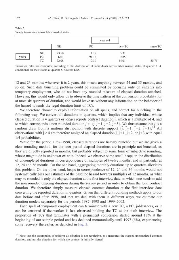
Table 2

Yearly transitions across labor market states

Transition rates are computed according to the distribution of individuals across labor market states at quarter t +4,

conditional on their status at quarter t. Source: EPA.


12 and 23 months; whenever it is 2 years, this means anything between 24 and 35 months, and

so on. Such data bunching problem could be eliminated by focusing only on entrants into

temporary employment, who do not have any rounded measure of elapsed duration attached.

However, this would only allow us to observe the time pattern of the conversion probability for

at most six quarters of duration, and would leave us without any information on the behavior of

the hazard towards the legal duration limit of TCs.

We therefore choose to exploit information on all spells, and correct for bunching in the

following way. We convert all durations in quarters, which implies that any individual whose

elapsed duration is 4 quarters or longer reports contract duration j, which is a multiple of 4, and

to which corresponds a non-rounded duration j a {j, j +1, j +2, j +3}. We thus assume that j is a

random draw from a uniform distribution with discrete support {j, j +1, j +2, j +3}.14 All

observations with jz4 are therefore assigned an elapsed duration j, j +1, j +2, or j +3 with equal

1/4 probabilities.

While for the period 1987–1998, elapsed durations are heavily bunched but we are given a

clear rounding method, for the later period elapsed durations are in principle not bunched, as

they are directly reported in months, but probably subject to some form of subjective rounding,

whose magnitude is unknown ex ante. Indeed, we observe some small heaps in the distribution

of uncompleted durations in correspondence of multiples of twelve months, and in particular at

12, 24 and 36 months. On the one hand, aggregating monthly durations up to quarters alleviates

this problem. On the other hand, heaps in correspondence of 12, 24 and 36 months would not

systematically bias our estimates of the baseline hazard towards multiples of 12 months, as what

may be rounded is only the elapsed duration at the first interview date, to which one needs to add

the non rounded ongoing duration during the survey period in order to obtain the total contract

duration. We therefore simply measure elapsed contract duration at the first interview date

converting the reported duration in quarters. Given that different rounding methods apply to our

data before and after 1998, and that we deal with them in different ways, we estimate our

duration models separately for the periods 1987–1998 and 1999–2002.

Each spell of temporary employment can terminate with a new TC, a PC, joblessness, or it

can be censored if the worker is last observed holding the TC at the sixth interview. The

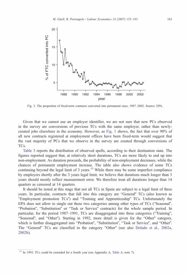
proportion of TCs that terminates with a permanent conversion started around 18% at the

beginning of our sample period and has declined monotonically until 1997 (6%), experiencing

some recovery thereafter, as depicted in Fig. 3.

14 Note that the assumption of uniform distribution is not restrictive, as j measures the elapsed uncompleted contract

duration, and not the duration for which the contract is initially signed.

% o

f FT

C c

onve

rted

into

PC

year1988 1990 1992 1994 1996 1998 2000 2002

5

10

15

20

Fig. 3. The proportion of fixed-term contracts converted into permanent ones, 1987–2002. Source: EPA.


Given that we cannot use an employer identifier, we are not sure that new PCs observed

in the survey are conversions of previous TCs with the same employer, rather than newly-

created jobs elsewhere in the economy. However, as Fig. 1 shows, the fact that over 90% of

all new contracts registered at employment offices have been fixed-term would suggest that

the vast majority of PCs that we observe in the survey are created through conversions of

TCs.

Table 3 reports the distribution of observed spells, according to their destination state. The

figures reported suggest that, at relatively short durations, TCs are more likely to end up into

non-employment. As duration proceeds, the probability of non-employment decreases, while the

chances of permanent employment increase. The table also shows evidence of some TCs

continuing beyond the legal limit of 3 years.15 While there may be some imperfect compliance

by employers shortly after the 3 years legal limit, we believe that durations much longer than 3

years should mostly reflect measurement error. We therefore treat all durations longer than 14

quarters as censored at 14 quarters.

It should be noted at this stage that not all TCs in Spain are subject to a legal limit of three

years. In particular, contracts that fall into this category are bGeneralQ TCs (also known as

bEmployment promotion TCsQ) and bTraining and ApprenticeshipQ TCs. Unfortunately the

EPA does not allow to single out these two categories among other types of TCs (bSeasonalQ,bProbationQ, bSubstitutionQ or bTask or ServiceQ contracts) for the whole sample period. In

particular, for the period 1987–1991, TCs are disaggregated into three categories (bTrainingQ,bSeasonalQ, and bOtherQ). Starting in 1992, more detail is given for the bOtherQ category,

which is further disaggregated into bProbationQ, bSubstitutionQ, bTask or ServiceQ, and bOtherQ.The bGeneralQ TCs are classified in the category bOtherQ (see also Dolado et al., 2002a,

2002b).

15 In 1993, TCs could be extended for a fourth year (see Appendix A, Table A, note 7).

Table 3

The duration distribution of fixed-term contracts, by state of exit

Duration (quarters) NE PC New TC Same TC Total No. of spells

1 54.33 10.13 13.69 21.85 47,622

2 34.67 8.73 38.80 17.80 38,684

3 28.81 10.67 37.92 22.59 20,751

4 19.53 11.92 46.28 22.27 16,295

5–8 15.53 12.89 27.03 44.55 23,101

9–12 15.90 20.78 22.68 40.64 7,775

N12 13.16 13.63 21.95 51.26 7,864

Total No. of spells 54,306 18,023 46,673 43,090 162,092

Each row sums to 100, with each entry giving the probability to exit into any of the four states, conditional on the contract

duration. All our rounded elapsed durations j are replaced with random draws from a uniform distribution with discrete

support {j, j +1, j +2, j+3}. Source: EPA.


The crucial question for the interpretation of our estimates is then how the inclusion of

contracts other than bGeneralQ and bTrainingQ TCs in our sample may affect our estimates.

Clearly, the inclusion of other types of contracts that do not have a three-year legal limit

would lower our estimate of the three-year spike. This can be seen more clearly by looking

at the conversion pattern of each type of contract for the period 1992–2002 (for which a

relatively more disaggregate information on type of contract is available in the EPA). Table 4

shows raw conversion rates by duration for each type of TC. The categories that have clear

spikes at 9–12 quarters (approaching the 3-year duration limit) are the seasonal and the

probation ones (that do not account for a large share of temporary employment anyway) and

the bOtherQ category. We are thus being conservative in estimating the three-year spike. Were

we able to single out bGeneralQ TCs for the whole sample period, we would have found an

even higher spike.

Explanatory variables included in our regressions are individual characteristics such as

gender, age, education, and marital status. Year dummies (referring to the year in which the

individual obtained a conversion or, in case of censoring, to the year in which she was last

interviewed) are also included in order to capture any time pattern in conversion probabilities

across the Spanish business cycle. Finally, sector dummies and the sectoral unemployment rate

Table 4

Permanent conversion rates by duration and type of contract, 1992–2002

duration

(quarters)

Training and

Apprent

Seasonal Other Probation Substitution Task or

Service

1 5.55 3.04 9.16 16.77 5.28 6.08

2 4.86 5.57 8.54 12.47 7.31 6.14

3 5.81 6.83 10.70 10.44 9.42 7.22

4 10.54 9.81 11.98 12.96 9.77 8.14

5–8 10.89 7.55 13.82 8.70 9.61 7.51

9–12 13.67 24.75 21.48 20.00 14.64 10.17

N12 9.83 6.80 6.82 0.00 2.10 4.71

All durations 7.12 4.79 10.63 13.48 7.12 6.91

All our rounded elapsed durations j are replaced with random draws from a uniform distribution with discrete support {j,

j +1, j+2, j +3}. Source: EPA.

Table 5

Sample characteristics of temporary workers

NE PC new TC same TC Total sample

Female 45.38 39.99 35.23 41.32 40.95

Age 16–24 yrs 41.24 35.96 41.74 41.51 40.87

Age 25–34 yrs 26.87 33.12 30.64 28.01 29.08

Age 35–44 yrs 15.94 16.49 15.76 16.53 16.21

Age 45+yrs 15.95 12.86 11.86 13.22 13.85

No qualification 14.97 8.66 8.05 10.52 11.17

Primary education 28.84 28.27 26.87 26.76 27.80

Secondary education 46.39 47.47 54.73 45.97 48.92

University education 9.52 13.98 10.28 15.82 11.95

Married 40.09 40.57 37.93 36.90 38.95

Agriculture 17.66 4.96 7.29 5.29 10.03

Manufacturing 15.66 22.23 22.15 18.48 19.06

Construction 15.93 12.92 18.86 19.68 17.48

Services 50.75 58.31 51.69 55.81 53.44

Average unemp. rate 12.54 10.89 13.09 11.13 12.19

Total No. of spells 54,306 18,023 46,673 43,090 162,092

All entries (except the average unemployment rate) indicate the percentage of workers with a given characteristic in the

sample. Standard deviations in parenthesis. Source: EPA.


(measured at the start of the survey period or at the start of the TC if this happened later) should

capture the effect of overall labor market performance, if any, on the conversion of contracts.

Average sample values of these variables are reported in Table 5, for both the whole sample and

each type of destination.

4. Econometric specification

The panel structure of the data set described requires a discrete time hazard function

approach, as outlined in Narendranathan and Stewart (1993) and Jenkins (1995).

Suppose that the transition out of temporary employment is a continuous process with

hazard

hi tjxið Þ ¼ k tð Þ exp xiVbð Þ; ð10Þ

where k(t) denotes the baseline hazard, x is a vector of time-invariant explanatory

variables, and b is a vector of unknown coefficients. The discrete time hazard denotes

the probability of a spell of temporary employment being completed by time t +1,

given that it was still continuing at time t. The discrete time hazard is therefore given

by

hi tjxið Þ ¼ 1� exp �Z tþ1

t

hi ujxið Þdu�¼ 1� exp � exp xiVbð Þc tð Þf g

�ð11Þ

where

c tð Þ ¼Z tþ1

t

k uð Þdu ð12Þ

denotes the integrated baseline hazard. We do not specify any functional form for c(t),and estimate the model semiparametrically.


The (log) likelihood contribution of a spell of length di is

Li ¼ cilnhi dijxið Þ þXdi�1t¼1

ln 1� hi tjxið Þ½ � ¼ ciln 1� exp � exp xiVbð Þc dið Þ½ �f g

�Xdi�1t¼1

exp xiVbð Þc tð Þ; ð13Þ

where ci is a censoring indicator that takes the value 1 if di is uncensored and zero otherwise.

We need to adapt the likelihood contribution (13) to our stock sample. As we observe spells

of temporary employment that started before the survey period, we use self-reported information

to find out the quarter in which these spells begun, and we condition transition rates on the

length of temporary employment at the first interview date. Suppose that an individual i enters

the survey after ji quarters of temporary employment and holds the TC for another ki quarters,

for a total duration di = ji +ki, that can be either censored or uncensored. The individual

likelihood contribution becomes

Li ¼ cilnhi ji þ kixið Þ þXjiþki�1

t¼jiþ1ln 1� hi tjxið Þf g

¼ ciln 1� exp � exp xiVbf gc ji þ ki jð Þ½ �ð Þ �Xjiþki�1

t¼jtþ1exp xiVbf gc tð Þ: ð14Þ

The baseline hazard can be estimated non-parametrically by maximizing the log-likelihood

L ¼Pn

i¼1 Li with respect to the g(d ) terms and the b vector. The vector of controls xi includes a

number of individual and job-related characteristics, which are treated as time invariant.

Appendix C explains in detail how this empirical specification can be brought to the data when

the available measure of duration is bunched.

We next make standard extensions to the econometric model outlined. First, as TCs can

terminate with the conversion into a PC or alternative states, we need to consider a competing

risk model, that distinguishes exits into permanent employment from exits into alternative

states. It can be shown that, if distinct destinations depend upon disjoint subsets of parameters,

the parameters of a given cause-specific hazard can be estimated by treating durations

finishing for other reasons as censored at time of exit (see Narendranathan and Stewart, 1993).

We therefore treat all temporary employment spells that end in a new TC or in non-

employment as censored at the time the first contract is terminated. Having said this, the semi-

parametric hazard specification (14) used for the single-risk model can be applied for the

permanent job hazard.

Finally, we control for the effect of possibly omitted regressors in the exit from fixed-term

employment by conditioning the hazard rate on an individual’s unobserved characteristics,

summarized into a random disturbance v. The conditional (discrete time) hazard rate is then

written as

hi tjxi; við Þ ¼ 1� exp � exp xiVbþ við Þc tð Þ½ � ð15Þ

with vi independent of xi and t. Note however that, in a competing risk framework, allowing for

a random disturbance term in each of the cause-specific hazards requires an additional


assumption, namely the independence of these disturbance terms across the cause-specific

hazards.16

The conditional likelihood contribution for the i th individual is the given by

Lijvi ¼ cilnhi ji þ kijxi; við Þ þPjiþki�1

t¼jiþ1 ln 1� hi tjxi; við Þf g. The unconditional likelihood contri-

bution (that depends on observable regressors only) is obtained by integrating the conditional

one over vi:

Li ¼Z

cilnhi ji þ kijxi; við Þ þXjiþki�1

t¼jiþ1ln 1� hi tjxi; við Þ½ �

( )f við Þdvi: ð16Þ

Among potential functional forms for f(vi), a very convenient candidate is the gamma

distribution, which delivers a closed form solution for (16) and therefore avoids numerical

integration (see Lancaster, 1979; see also Han and Hausman, 1990; Dolton and O’Neill, 1996,

for an application of gamma-distributed unobserved heterogeneity to discrete time hazard

models).

Under these assumptions the individual likelihood contribution is given by

Li ¼ ln 1þ r2Xjiþki�1

t¼jiþ1exp xiVbð Þc tð Þ

" #�1=r2

� ci 1þ r2Xjiþki

t¼jiþ1exp xiVbð Þc tð Þ

" #�1=r28<:

9=;;ð17Þ

where j2 is an extra parameter to be identified.

5. Empirical results

We move on to estimating the econometric model outlined in the previous Section, for the

determinants of worker transitions from temporary to permanent employment. The results of our

estimates are reported in Table 6. These estimates refer to the sample period 1987–1998, for

which we have a consistent measure of contract duration. Separate estimates for the later period

are reported further down in Table 10. Two specifications of our regression equation are

provided. In the first one we do not allow for unobserved heterogeneity among individuals. In

the second one we control for the effect of possibly omitted regressors by allowing for a

Gamma-distributed disturbance term.

The effect of several individual characteristics on conversion probabilities are fairly standard,

and consistent with previous results obtained from logit estimates (see Alba, 1998). Column I of

Table 6 shows that the probability of a permanent conversion increases with age up to prime age

and stays constant afterwards. Being married positively affects the probability of obtaining a

permanent contract. Gender and education have the expected effects on conversion rates,

although they are not significantly different from zero. Industry dummies show that conversion

rates are highest in services and lowest in construction. Time fixed-effects imply in turn a

roughly monotonically decreasing trend in the proportion of TCs being converted on a

permanent basis. Such trend is stronger in the first half of the sample period and then fades away

16 The alternative approach would be to assume perfect correlation (as opposed to zero correlation) between the cause-

specific disturbance terms (see Narendranathan and Stewart, 1993, for a discussion of advantages and disadvantages of

the two methods).

Table 6

Maximum likelihood estimates of the transition from temporary to permanent employment: 1987:2–1998:4

I II

Characteristics

Female �0.019 (0.018) �0.015 (0.021)

Age 25–34 yrs 0.194 (0.023) 0.225 (0.025)

Age 35–44 yrs 0.152 (0.030) 0.191 (0.036)

Age 45+yrs 0.135 (0.033) 0.170 (0.041)

Secondary education �0.014 (0.021) �0.022 (0.025)

University education 0.015 (0.032) 0.015 (0.037)

Married 0.101 (0.022) 0.120 (0.026)

Manufacturing 0.108 (0.037) 0.085 (0.056)

Construction �0.216 (0.023) �0.280 (0.052)

Services 0.231 (0.037) 0.252 (0.055)

Year 1988 �0.085 (0.047) �0.138 (0.058)

Year 1989 �0.333 (0.045) �0.456 (0.058)

Year 1990 �0.520 (0.047) �0.693 (0.057)

Year 1991 �0.490 (0.048) �0.707 (0.058)

Year 1992 �0.678 (0.040) �0.896 (0.056)

Year 1993 �0.675 (0.042) �0.885 (0.072)

Year 1994 �0.765 (0.044) �1.005 (0.075)

Year 1995 �0.729 (0.044) �0.958 (0.069)

Year 1996 �0.863 (0.040) �1.109 (0.062)

Year 1997 �1.091 (0.047) �1.372 (0.064)

Year 1998 �1.122 (0.047) �1.414 (0.059)

Year 1999 �1.099 (0.071) �1.350 (0.085)

Log log unemployment rate �0.271 (0.057) �0.337 (0.103)

Base line hazard steps

Step 1 0.075 (0.007) 0.082 (0.018)

Step 2 0.074 (0.007) 0.090 (0.020)

Step 3 0.068 (0.007) 0.091 (0.020)

Step 4 0.094 (0.009) 0.138 (0.029)

Step 5 0.078 (0.008) 0.124 (0.028)

Step 6 0.061 (0.007) 0.097 (0.023)

Step 7 0.072 (0.008) 0.110 (0.024)

Step 8 0.105 (0.013) 0.111 (0.026)

Step 9–11 0.055 (0.006) 0.095 (0.023)

Step 12 0.147 (0.017) 0.214 (0.050)

Step 13–14 0.068 (0.007)

r2 1.421 (0.110)

Mean log-likelihood �0.358 �0.353No. of obs. 125,077 125,077

(1) Standard errors in parenthesis; (2) Source: EPA.


in the late 1990s, consistently with what we observed in the raw data of Fig. 3. Finally, sectoral

unemployment has a negative and significant impact on conversion rates. As lower

unemployment implies better outside opportunities for temporary workers in search for better

jobs, it enables them to more credibly threat their employer in case of low conversion prospects.

This is in line with prediction (4) of Section 2. Very similar results (nor reported here) were

obtained when using time-varying unemployment rates instead of time invariant. This is not

surprising, in the light of the relatively strong persistence of Spanish unemployment at the

quarterly frequencies.

duration

Baseline hazard, No unob het Baseline hazard, With unob het

1 2 3 4 5 6 7 8 9 10 11 12 13 14

.05

.15

.25

.35

.45

Fig. 4. Predicted hazard for the transition from TC to PC, 1987–1998 (see Table 6). Reference category: male, not

married, aged 16–24, secondary education, employed in services, started TC in 1987.


The quarterly steps of the baseline hazard are reported at the bottom of Table 6. In the

estimates provided we impose a constant hazard across steps 9–11 and steps 13–14,

respectively.17 Above 8 quarters of contract duration, step 12 was the only one that was

individually identified. As step 12 coincides with the 3-year legal limit of TCs, the relatively

higher density of completed spells at this duration allowed us to identify this step separately

from adjacent ones.

The parallel estimation that controls for the effect of unobserved heterogeneity is represented

in column II of Table 6. The positive and significant variance of the Gamma distributed

disturbance shows that there is some residual heterogeneity among individuals, which is not

properly accounted for by included regressors. However, the partial effect of most regressors

remains practically unchanged if compared with the case where no unobserved heterogeneity is

accounted for, as does the global fit of the regression. As there is no major difference between

the estimates of column I and II,18 and the additional restrictions embodied in specification II

seem largely unnecessary, in the regressions that follow we do not allow for unobserved

heterogeneity in our estimates.

The predicted hazards corresponding to regressions I and II of Table 6 are plotted in Fig. 4

for a typical temporary worker (single male, aged 16–24, with completed secondary education,

employed in the service sector). Controlling for the presence of unobserved heterogeneity in

regression II simply scales upward the whole hazard, as it is reasonable to expect, but hardly

changes its overall time pattern. It can be noted that, with both specifications, the hazard has

some spikes at durations around one, two and three years. This denotes substantial

heterogeneity in the time pattern of conversion rates and is consistent with prediction (1) of

17 We first attempted to estimate the fully unrestricted model with 14 baseline steps and found that steps 9–11 were not

separately identifiable, and similarly for steps 13 and 14. See Appendix C for a formal discussion of identification

problems.18 The only change from column I is that step 13 and 14 are not even jointly identified (and when we attempted to identify

them, the corresponding coefficient was virtually zero and the others very close to those reported in column II of Table 6).

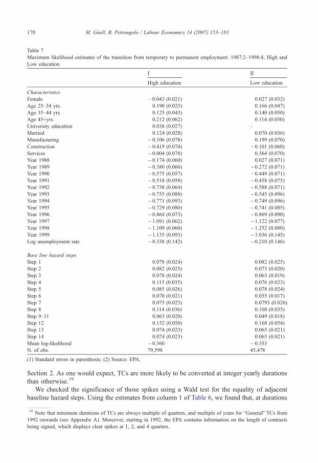
Table 7

Maximum likelihood estimates of the transition from temporary to permanent employment: 1987:2–1998:4; High and

Low education

I II

High education Low education

Characteristics

Female �0.043 (0.021) 0.027 (0.032)

Age 25–34 yrs. 0.190 (0.025) 0.166 (0.047)

Age 35–44 yrs. 0.125 (0.043) 0.140 (0.050)

Age 45+yrs. 0.212 (0.062) 0.114 (0.050)

University education 0.038 (0.027) –

Married 0.124 (0.028) 0.070 (0.036)

Manufacturing �0.106 (0.078) 0.199 (0.070)

Construction �0.419 (0.074) �0.101 (0.060)

Services �0.004 (0.078) 0.364 (0.070)

Year 1988 �0.174 (0.060) 0.027 (0.071)

Year 1989 �0.380 (0.060) �0.272 (0.071)

Year 1990 �0.575 (0.057) �0.449 (0.071)

Year 1991 �0.518 (0.058) �0.458 (0.075)

Year 1992 �0.738 (0.064) �0.588 (0.071)

Year 1993 �0.755 (0.088) �0.545 (0.096)

Year 1994 �0.771 (0.093) �0.749 (0.096)

Year 1995 �0.729 (0.080) �0.741 (0.085)

Year 1996 �0.864 (0.073) �0.869 (0.090)

Year 1997 �1.091 (0.062) �1.122 (0.077)

Year 1998 �1.109 (0.060) �1.252 (0.080)

Year 1999 �1.135 (0.093) �1.036 (0.145)

Log unemployment rate �0.338 (0.142) �0.210 (0.146)


Step 1 0.078 (0.024) 0.082 (0.025)

Step 2 0.082 (0.025) 0.073 (0.020)

Step 3 0.078 (0.024) 0.063 (0.019)

Step 4 0.115 (0.035) 0.076 (0.023)

Step 5 0.085 (0.026) 0.078 (0.024)

Step 6 0.070 (0.021) 0.055 (0.017)

Step 7 0.075 (0.023) 0.0793 (0.026)

Step 8 0.114 (0.036) 0.108 (0.035)

Step 9–11 0.063 (0.020) 0.049 (0.018)

Step 12 0.152 (0.050) 0.168 (0.054)

Step 13 0.074 (0.023) 0.065 (0.021)

Step 14 0.074 (0.023) 0.065 (0.021)

Mean log-likelihood �0.360 �0.353N. of obs. 79,598 45,478



Section 2. As one would expect, TCs are more likely to be converted at integer yearly durations

than otherwise.19

We checked the significance of those spikes using a Wald test for the equality of adjacent

baseline hazard steps. Using the estimates from column 1 of Table 6, we found that, at durations

19 Note that minimum durations of TCs are always multiple of quarters, and multiple of years for bGeneralQ TCs from1992 onwards (see Appendix A). Moreover, starting in 1992, the EPA contains information on the length of contracts

being signed, which displays clear spikes at 1, 2, and 4 quarters.


around one year, the baseline hazard at 4 quarters is significantly higher than both the one at 3

quarters (v2=70.97, against the critical value v2(1, 0.05)=3.84), and the one at 5 quarters

(v2=27.69). At durations around two years, the baseline hazard at 8 quarters is significantly

higher than both the one at 7 and the one at 9–11 quarters (v2=13.68 and v2=37.30,

respectively). Finally, at duration around three years, the baseline hazard at 12 quarters is

significantly higher than both the previous and the later one (v2=37.30 and v2=33.57;

respectively). Also, while the spikes at one and two years are not significantly different from

each other (v2=2.25), the one at three years is significantly higher than both of them (v2=13.09

and v2=25.23; respectively). Using the estimates from column 2 of Table 6, which control for

unobserved heterogeneity, the spike at two years disappears, as the step at 8 quarters is not

significantly different from adjacent ones, and we are left with an early and a late spike in

permanent conversions, around durations of one and three years respectively. As with the

previous estimates, the baseline hazard at three years is significantly higher than at both one and

two years. Substantial time variation in conversion rates, and especially the coexistence of early

and late spikes, are consistent with prediction (1) of Section (2).

Different population groups have different employment prospects and unemployment rates,

which affect their outside options and thus their bargaining power on temporary jobs. In

particular, skilled workers have lower unemployment rates than the less-skilled (see Dolado et

al., 2002b), and Spanish women have higher unemployment rates than males (see Azmat et al.,

in press). We thus estimate separate duration models of temporary employment for men and

women, the skilled and the unskilled.

We first split our sample along the educational dimension, and define as skilled all workers

who have completed secondary education. Table 7 shows that while skilled women have lower

conversion rates than skilled men, no significant gender differences can be detected among the

less-skilled. The steps of the baseline hazard are shown in the lower part of the Table, and the

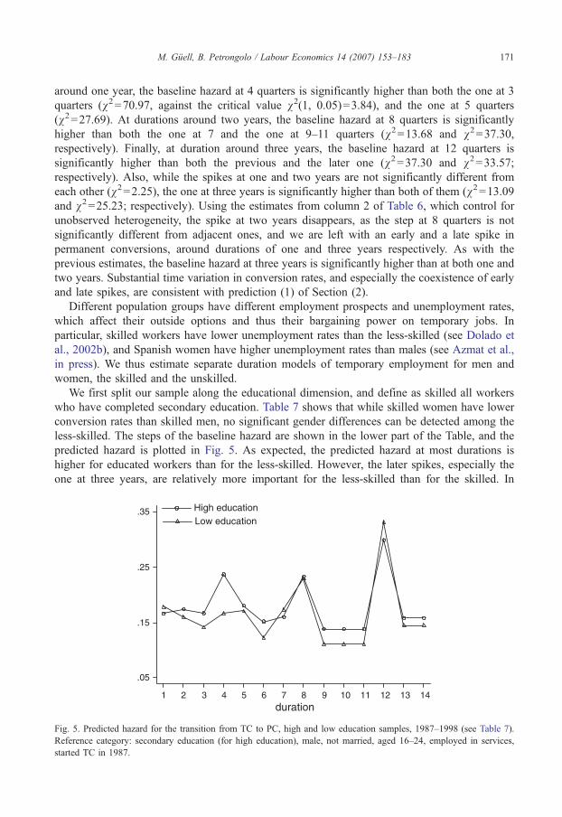
predicted hazard is plotted in Fig. 5. As expected, the predicted hazard at most durations is

higher for educated workers than for the less-skilled. However, the later spikes, especially the

one at three years, are relatively more important for the less-skilled than for the skilled. In

duration

High education Low education

1 2 3 4 5 6 7 8 9 10 11 12 13 14

.05

.15

.25

.35

Fig. 5. Predicted hazard for the transition from TC to PC, high and low education samples, 1987–1998 (see Table 7)

Reference category: secondary education (for high education), male, not married, aged 16–24, employed in services

started TC in 1987.

.

,


particular, there is really no early spike for the less-skilled, as the predicted hazard at 4 quarters is

not significantly different from the one at 5 quarters and the one at 8 quarters is not significantly

different from the one at 7 quarters. The fact that the time pattern of renewals is everywhere

lower and more strongly increasing for the less-skilled than for the skilled is in line with

prediction (2) of Section (2): skilled workers tend to occupy more productive job matches, which

are thus more likely to be converted before the legal limit. Also, one would expect that the less

skilled are generally in a weaker bargaining position than the skilled, as they may be more easily

replaced. Moreover, in a high unemployment scenario, the skilled may take up unskilled jobs,

Table 8

Maximum likelihood estimates of the transition from temporary to permanent employment: 1987:2–1998:4; Males and

Females

I II

Males Females

Characteristics

Age 25–34 yrs 0.201 (0.029) 0.165 0.034

Age 35–44 yrs 0.171 (0.039) 0.085 (0.047)

Age 45+yrs 0.108 (0.044) 0.141 (0.054)

Secondary education 0.039 (0.027) �0.117 (0.033)

University education 0.164 (0.046) �0.153 (0.038)

Married 0.149 (0.028) 0.047 (0.032)

Manufacturing 0.120 (0.057) 0.052 (0.109)

Construction �0.235 (0.049) 0.282 (0.145)

Services 0.194 (0.057) 0.260 (0.107)

Year 1998 �0.001 (0.059) �0.226 (0.077)

Year 1989 �0.285 (0.060) �0.413 (0.075)

Year 1990 �0.490 (0.060) �0.560 (0.074)

Year 1991 �0.408 (0.061) �0.605 (0.071)

Year 1992 �0.700 (0.057) �0.633 (0.076)

Year 1993 �0.669 (0.083) �0.649 (0.107)

Year 1994 �0.780 (0.080) �0.701 (0.120)

Year 1995 �0.778 (0.074) �0.625 (0.108)

Year 1996 �0.914 (0.064) �0.758 (0.086)

Year 1997 �1.116 (0.063) �1.021 (0.087)

Year 1998 �1.143 (0.057) �1.066 (0.078)

Year 1999 �1.092 (0.105) �1.103 (0.113)

Log unemployment rate �0.261 (0.122) �0.351 0.185


Step 1 0.071 (0.018) 0.069 (0.028)

Step 2 0.072 (0.018) 0.066 (0.026)

Step 3 0.066 (0.017) 0.062 (0.025)

Step 4 0.087 (0.022) 0.092 (0.037)

Step 5 0.073 (0.018) 0.074 (0.030)

Step 6 0.054 (0.014) 0.063 (0.026)

Step 7 0.062 (0.016) 0.076 (0.031)

Step 8 0.117 (0.032) 0.075 (0.032)

Step 9–11 0.047 (0.012) 0.059 (0.025)

Step 12 0.173 (0.049) 0.095 (0.042)

Step 13–14 0.071 (0.018) 0.053 (0.021)

Mean log-likelihood �0.362 �0.351No. of obs. 75,527 49,550



crowding out the less-skilled of their usual occupations (see Dolado et al., 2002b). In this sense,

these results empirically support prediction (4) of Section 2. Screening and early conversions for

successful workers are also more likely to apply to the skilled rather than the less-skilled, and

this is again confirmed in our estimates.

Some gender differences in conversion rates are detected in Table 8. While age effects are

similar for men and women, education has a positive effect on male conversion rates, but a

negative effect on female ones, and this could explain the non-significant effect found in Table 6.

As education presumably enhances productivity and a worker’s outside options, we find that it has

the expected impact on male conversion rates but not on female ones, as if other unmeasured

factors such as, say, labor market attachment, were more relevant than observable human capital

for women’s promotions. It seems moreover that, in the interim period between the two reforms,

conversion rates keep falling for males, while stabilizing for females. The unemployment rate has

similar qualitative impact on conversion rates across genders, if anything stronger for females.

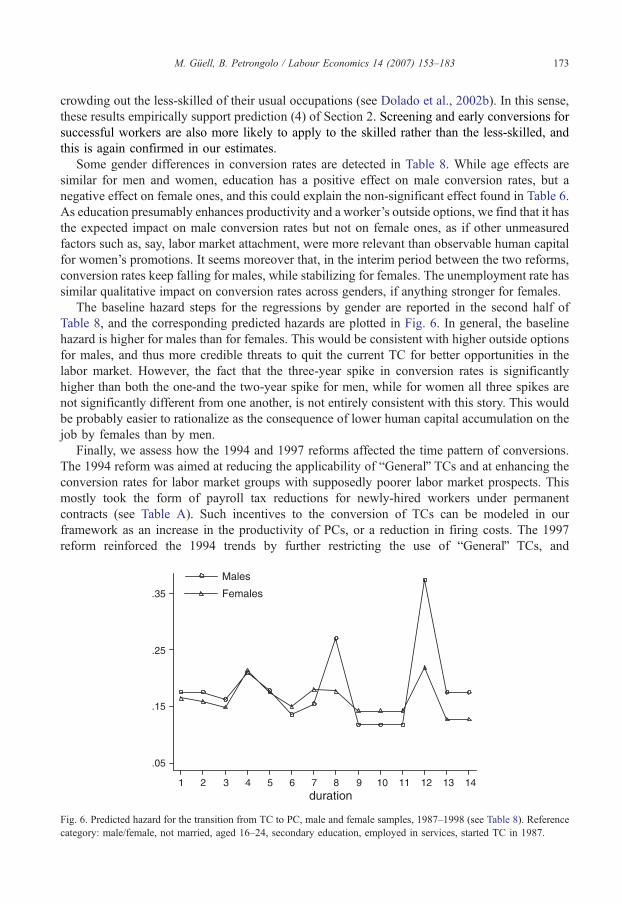
The baseline hazard steps for the regressions by gender are reported in the second half of

Table 8, and the corresponding predicted hazards are plotted in Fig. 6. In general, the baseline

hazard is higher for males than for females. This would be consistent with higher outside options

for males, and thus more credible threats to quit the current TC for better opportunities in the

labor market. However, the fact that the three-year spike in conversion rates is significantly

higher than both the one-and the two-year spike for men, while for women all three spikes are

not significantly different from one another, is not entirely consistent with this story. This would

be probably easier to rationalize as the consequence of lower human capital accumulation on the

job by females than by men.

Finally, we assess how the 1994 and 1997 reforms affected the time pattern of conversions.

The 1994 reform was aimed at reducing the applicability of bGeneralQ TCs and at enhancing the

conversion rates for labor market groups with supposedly poorer labor market prospects. This

mostly took the form of payroll tax reductions for newly-hired workers under permanent

contracts (see Table A). Such incentives to the conversion of TCs can be modeled in our

framework as an increase in the productivity of PCs, or a reduction in firing costs. The 1997

reform reinforced the 1994 trends by further restricting the use of bGeneralQ TCs, and

duration

Males

Females

1 2 3 4 5 6 7 8 9 10 11 12 13 14

.05

.15

.25

.35

Fig. 6. Predicted hazard for the transition from TC to PC, male and female samples, 1987–1998 (see Table 8). Reference

category: male/female, not married, aged 16–24, secondary education, employed in services, started TC in 1987.

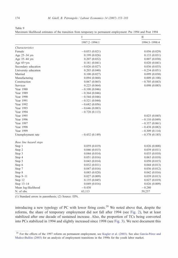
Table 9

Maximum likelihood estimates of the transition from temporary to permanent employment: Pre 1994 and Post 1994

I II

1987:2–1994:1 1994:3–1998:4

Characteristics

Female �0.053 (0.021) 0.056 (0.029)

Age 25–34 yrs 0.199 (0.026) 0.133 (0.031)

Age 35–44 yrs 0.207 (0.032) 0.007 (0.030)

Age 45+yrs 0.181 (0.041) 0.020 (0.041)

Secondary education �0.026 (0.027) 0.036 (0.035)

University education 0.203 (0.040) �0.234 (0.051)

Married 0.100 (0.027) 0.099 (0.030)

Manufacturing 0.094 (0.060) 0.009 (0.100)

Construction 0.067 (0.065) �0.705 (0.043)

Services 0.225 (0.064) 0.098 (0.085)

Year 1988 �0.108 (0.046)

Year 1989 �0.364 (0.046)

Year 1990 �0.544 (0.046)

Year 1991 �0.521 (0.044)

Year 1992 �0.682 (0.056)

Year 1993 �0.646 (0.083)

Year 1994 �0.728 (0.113)

Year 1995 0.025 (0.045)

Year 1996 �0.110 (0.049)

Year 1997 �0.357 (0.061)

Year 1998 �0.438 (0.082)

Year 1999 �0.309 (0.114)

Unemployment rate �0.432 (0.149) �0.378 (0.185)


Step 1 0.059 (0.019) 0.026 (0.008)

Step 2 0.046 (0.015) 0.039 (0.011)

Step 3 0.044 (0.014) 0.035 (0.010)

Step 4 0.051 (0.016) 0.063 (0.018)

Step 5 0.043 (0.014) 0.050 (0.015)

Step 6 0.032 (0.011) 0.044 (0.013)

Step 7 0.047 (0.016) 0.036 (0.012)

Step 8 0.085 (0.028) 0.042 (0.016)

Step 9–11 0.027 (0.009) 0.039 (0.013)

Step 12 0.135 (0.045) 0.027 (0.019)

Step 13–14 0.049 (0.016) 0.026 (0.009)

Mean log-likelihood �0.430 �0.280N. of obs. 63,113 59,257



introducing a new typology of PC with lower firing costs.20 We noted above that, despite the

reforms, the share of temporary employment did not fall after 1994 (see Fig. 2), but at least

stabilized after one decade of sustained increase. Also, the proportion of TCs being converted

into PCs stabilized in 1994 and slightly increased since 1998 (see Fig. 3). We next document this

20 For the effects of the 1997 reform on permanent employment, see Kugler et al. (2003). See also Garcıa-Perez and

Munoz-Bullon (2003) for an analysis of employment transitions in the 1990s for the youth labor market.

duration

Pre 1994

Post 1994

1 2 3 4 5 6 7 8 9 10 11 12 13 14

.05

.15

.25

.35

Fig. 7. Predicted hazard for the transition from TC to PC, contracts started before and after 1994 (see Table 9). Reference

category: male, not married, aged 16–24, secondary education, employed in services, started TC in 1987 (for pre 1994

sample) and started TC in 1994 (for post 1994 sample).

21 As the reform was passed in May 1994, it is not clear whether the old or the new legislation applies to contracts

signed exactly in 1994:2, and we therefore drop them from our sample.


trend in conversion rates, and check whether such overall tendency conceals diverging patterns

for different labor market segments.

We split our sample into two subperiods, corresponding to different institutional environ-

ments. These are 1987:2-1994:1 and 1994:3-1998:4.21 Temporary spells are allocated to these

subperiods according to their starting quarter, or the first survey quarter if the contract had

already started at the first survey date. Although there was a reform in 1997, we provide pooled

estimates for the post 1994 period for two reasons. First, the 1997 reform did not imply any

major discontinuity with respect to the 1994 reform as far as the conversion of TCs was

concerned, and basically strengthened the incentives to permanent conversions of TCs. Second,

the post 1997 period would be rather short, from 1998:1 to 1998:4, and would not allow us to

identify the baseline hazard steps for durations longer than one year.

In Table 9 we report results for the pre and the post 1994 periods. Our estimates clearly

show that permanent conversion prospects of women, the less educated and younger workers

have improved after 1994. The female dummy switches from negative and significant in the

first sub-period, to positive and significant in the second one, and the reverse is true for the

university education dummy. Conversion rates are reduced for those aged 25–34 and even more

older workers. Interestingly, before 1994 conversion rates are highest for the middle age

category 35–44, but they drop to the same level as for the 16–24 category with the reform.

Targeting subsidies to the conversion of contracts for women (in occupations in which they are

under-represented) and young workers seems to have been effective in enhancing their

prospects of accessing permanent employment. Also, conversion rates after 1994 have strongly

deteriorated in construction.

Clearly, the time pattern of conversions is greatly affected after the 1994 reform, as

shown in the lower part of Table 9 and in Fig. 7. Before 1994, clear spikes can be detected


in conversion rates around 1, 2 and 3 years, each of them being higher than the previous

one at conventional significance levels. In particular, the permanent conversion probability

for the reference worker after 3 years of temporary employment is twice as high as the one

at one year. Interestingly, after the 1994 reform, there is a small spike in conversion rates at

one year, and after that conversion rates decline steadily, without any later spike. One the

one hand, it can be concluded that the 1994 reform has successfully affected the use of TCs

in the sense of inducing employers to earlier rather than later conversions- consistently with

predictions (2) and (3) of Section 2. On the other hand, it can be clearly noted that, except

at durations of 9–11 quarters, the conversion rates after 1994 are always lower than the ones

for the earlier period. While affecting the time pattern of conversions, the 1994 reform

failed quite badly at pushing higher their average level. One possible reason for this can be

found in the changing composition of temporary employment after 1994. The 1994 reform

limited substantially the applicability of bGeneralQ TCs, which were those initially conceived

by the legislator for being converted into PCs. With a declining share of bGeneralQ TCs in

total temporary employment, and an increasing share of bTask or ServiceQ contracts, it is

probably not surprising that average renewal rates also declined.

Table 10

Maximum likelihood estimates of the transition from temporary to permanent employment: 1999:1–2002:4

Characteristics

Female �0.090 (0.034)

Age 25–34 yrs 0.035 (0.038)

Age 35–44 yrs �0.228 (0.056)

Age 45+yrs �0.255 (0.063)

Secondary education 0.112 (0.039)

University education 0.035 (0.041)

Marrried 0.079 (0.042)

Manufacturing 0.751 (0.265)

Construction �0.418 (0.168)

Services 0.636 (0.213)

Year 2000 0.073 (0.048)

Year 2001 0.085 (0.088)

Log unemployment rate �0.121 (0.290)


Step 1 0.016 (0.008)

Step 2 0.026 (0.013)

Step 3 0.023 (0.012)

Step 4 0.038 (0.020)

Step 5 0.031 (0.016)

Step 6 0.026 (0.014)

Step 7 0.026 (0.013)

Step 8 0.042 (0.022)

Step 9 0.032 (0.017)

Step 10 0.016 (0.008)

Step 11 0.015 (0.008)

Step 12 0.022 (0.012)

Step 13 0.016 (0.008)

Step 14 0.011 (0.006)

Mean log-likelihood �0.402N. of obs. 37,015


Pos

t 199

8

duration1 2 3 4 5 6 7 8 9 10 11 12 13 14

.05

.1

.15

Fig. 8. Predicted hazard for the transition from TC to PC, 1999–2002 (see Table 10). Refeerence category: male, not

married, aged 16–24, secondary education, employed in services, started TC in 1999.


For the last 3 years of our sample, corresponding to 1999–2002, the duration of temporary

employment spells is measured differently from the previous period, as explained in detail in

Section 3, and duration data are therefore not directly comparable. In particular, as durations are

measured more precisely, we manage to separately identify all quarterly steps in the baseline

hazard. We therefore provide separate estimates for this later period in Table 10 and Fig. 8. The

most noticeable difference from the 1994–1998 period is age effects turning strongly negative

from age 35, possibly due to the impact of the 1990s reforms, targeted at permanent employment

prospects of youths. Also, the gender dummy is now negative and significant, while the impact

of the unemployment rate becomes non-significantly different from zero. Finally, the level of

conversion rates is lower than in the earlier subsample in correspondence of all durations. At the

same time, the third spike becomes lower than the previous two. The same tendency towards

lower but flatter conversion rates that we found for the 1994–1998 period is also detected for this

final subsample.

6. Conclusions

Given that most accessions to permanent employment in Spain happen through TCs, the

conversion of TCs into PCs is a key aspect of labor market segregation among Spanish

workers and of the overall performance of the Spanish labor market. This paper has studied

the determinants and the timing of the conversion of TCs into PCs in Spain using panel data

for the period 1987–2002, to shed light on the potential of temporary employment as a

stepping stone for stable, regular jobs. Specifically, we estimated a duration model for

temporary employment, with flexible duration dependence for the permanent employment

hazard.

We argued that the level and the timing of permanent promotions of TCs can be suggestive of

different levels of workersT outside options. Using a simple framework for firm’s choice of

conversion rates, we have argued that conversion rates should be higher for workers who can

credibly threat their employer to quit a temporary job. Finally, the pattern of renewals should be

Table A

Summary of Legislation on TCs in Spain

Month/Year Contractsintroduceda

Limits on duration Eligible workersb Indemnities attermination

Subsidies to firms

Minimum Maximum

03/1980 PC indefinite { 20 (45) days’wage peryear worked if fair (unfair)c

“Causal” TC limitedd

TrainingTC – 1 year { Secondary edu. degree or aboveobtained in thelast 2yrs.

Apprenticeship TC – 2 years { Aged 16-18 (except for disabled)with < secondary edu.

08/1984 General TC 6 months 3 years Any unemployed workere { 12 days’ wage per year workedf

Training TC 3 months 3 years { Secondary edu. degree or above obtained in the last 4yrs.

Apprenticeship TC 3 months 3 years { Aged 16-20 (except for disabled)with < secondary edu.

07/1992 General TC 1 year 3 yearsg Same as in 1984

05/1994 General TC 1 year 3 years { Unemployed aged >45, disabled, LTUh

Any firm starting a new economic activity Same as in 1984 {Fiscal incentives to hire eligible-UI recipients and to transform TC into PCfor aged <25 or >45, females,i disabled

Training TC 6 months 2 years Same as in 1984 If they transform TC into PCApprenticeship TC 6 months 3 years Same as in 1984

12/1997 New PC indefinite { Unemployed aged 18-29 or >45, LTU,disabled, TC since 05/1997j { 20 (33) days’ per year

worked if fair (unfair)c { Fiscal incentives to hire eligible workers,and to transform TC into New PC

General TC 1 year 3 years Disabled workers If they transform TC into New PCTraining TC 6 months 2 years Same as in 1984 If they transform TC into New PCApprenticeship TC 6 months 2 years Same as in 1984 If they transform TC into New PC

07/2001 New PC indefinite { Aged 16-29 o r>45, females,h

unemp. w/ dur. >6months, disabled Same as in 1997 { Fiscal incentives to hire eligible workers;transform TC into New PC

General TC 1 year 3 years Disabled workers 8 days per year workedf If they transform TC into New PCTraining TC 6 months 2 years Same as in 1984 If they transform TC into New PCApprenticeship TC 6 months 2 years Same as in 1984 If they transform TC into New PC

M.Guell,

B.Petro

ngolo

/LabourEconomics

14(2007)153–183

178


steeper for workers with lower outside options. We find that these predictions are broadly

confirmed by the estimates of our duration model for temporary employment, which delivers a

clear spike at the legal limit, and higher conversion rates in cases where workers supposedly

have higher outside options.

The likely role of worker outside options is more clearly visible when we estimate

separate conversion rates by education, as conversion rates are lower and more steeply

increasing with tenure on temporary jobs for the less-skilled. The results are less clear-cut

when we estimate separate conversion rates by gender. Men have higher conversion rates,

and presumably better employment prospects than women in the Spanish labor market.

However, the fact that the time pattern of conversions is less steep for women would point in

the opposite direction if one were to assess conversion rates solely on the basis of workers’

threat to quit. When comparing conversion rates for men and women it is likely that other

factors play an important role over and above outside labor market options, namely

noneconomic reasons for quits (see Manning, 2003, chapter 7), and thus different job

attachment for the two genders.

Acknowledgements

We wish to thank Manuel Arellano, Samuel Bentolila, Olimpia Bover, Andrea Ichino,

Alan Manning, Steve Nickell, Gilles Saint-Paul, the editors Andrea Ichino and Juan Dolado

and two anonymous referees for very useful comments. M. Guell acknowledges financial

support from the Spanish Ministry of Science and Technology & FEDER (Project BEC2003-

00412) and B. Petrongolo acknowledges financial support from the Spanish Ministry of

Education (Grant No. DGES PB97-0091).

Notes to Table A:aIf not stated otherwise, contracts introduced previously remain available.bAs a general principle for eli gibility for all types of TCs introduced in 1984, workers have a maximum 3 year limit

of continuous temporary employment with one or several employers. If a worker has been continuously employed on

TCs for 3 years, she needs to wait 12 months before being eligible for a new one. Similarly, for firms this limit binds

for a given job, in the sense that they cannot cover the same position for more than 3 years with TCs. Also, firms

cannot hire a temporary worker if they have reduced their workforce for economic reasons or their dismissals have

been declared unfair in the previous 12 months (in practice, it is difficult to assess whether these rules have been

effectively enforced).cThe fair (unfair) indemnity can be paid for a max. of 12 months (24 months). In case of unfair, forgone wages are al so

paid. Workers can be fired for disciplinary reasons (without indemnity) or economic reasons (indemnites indicated in

table). Workers always have the right to sue the employer if she disagrees with the dismissal case. Once the case is taken

to court, it can be declared fair or unfair. Around 72% of cases that go to court are declared unfair (see Galdon-Sanchez

and Guell, 2000).dDifferent limits apply to different types of causal TCs. For a specific project: indeterminated but limited. For

replacement: durati on of leave. For transitory production ci rcumstances: max 6 months in a year.eWorkers can be hired to undertake the normal activity of the firm or a any new economic activity.fIndemnities to be paid upon expiry of contract. There is no right to sue the employer for unfair dismissal in this case.gTCs which lasted 3 years and expire between march 3rd and december 31st, 1993, can be extended to a 4th year. After 4

years, firms get a subsidy if they convert the TC into a PC.hLTU refers to long-term unemployed (12 or more months in unemployment).iFemales in professions or jobs in which they are underepresented.jRoyal Decree Laws 8/97 and 9/97 were approved in May before the December law. The respecti ve laws from each

reform are: law 8/80 (Estatuto de los Trabajadores), law 32/84, law 22/92, laws 10/94 and 11/94; laws 63/1997, 64/97 and

66/97; law 12/2001.


Appendix A. The institutional background

Current legislation on labor contracts is contained in the Worker’s Statute (Estatuto de los

Trabajadores, ET) of 1980, which has since been modified on four occasions with the 1984, the

1994, 1997 and 2001 reforms. The ET of 1980 established priority to contracts of indefinite

duration and allowed TCs only for jobs that were temporary in their nature (like for particular

projects, e.g. constuction; or seasonal jobs, e.g. tourism). Some forms of training contracts for

young, first-time job seekers were also allowed (apprenticeship contracts and training contracts).

Other situations in which TCs were allowed was for eventual increases in demand or

replacement of a permanent worker in case of absence or temporary suspension of contract. The

ET also established the possibility for the Government to use TCs as an incentive to promote

employment. Except in this last situation, a specific cause was generally required in order to sign

a TC (bcausalQ TC).The 1984 reform exploits this last possibility in an extreme way, and introduces flexibility by

extending the applicability of TCs. It introduces a new bGeneralQ TC, as well as making training

contracts more flexible. After the reform, any worker can be hired on a temporary basis without

the requirement of a specific cause. This implies that for any job, employers can freely choose

between a PC or a TC. The 1994, 1997 and 2001 reforms have restricted the applicability of TC

and introduced subsidies for their conversion into PCs. Table A summarizes the relevant aspects

of the Spanish legislation on temporary employment during the past 20 years. TCs can be

characterized according to: i) limits on their duration (upon expiry, it is not possible to retain the

worker under a TC: either the worker is promoted to a PC or dismissed); ii) eligibility conditions

for workers; iii) indemnities at their termination; and iv) subsidies to firms.

Appendix B. Possible extensions to the theoretical frame-work

The simple framework of Section 2 can be extended in a number of ways. First, if wagesare

endogenized, they presumably respond to productivity, firing costs, and workers’ outside

options. In this case changes in productivity induce changes in wages. In order to ensure

BR2*=Bpi N0 one simply needs wages adjusting less than one for one to productivity changes. In

order to ensure BR1*=BpiN0, one also needs the impact of productivity on wages on PCs to be

not too large with respect to the corresponding impact on wages on TCs. A natural way to

endogenize wages in this framework would be to introduce a Nash sharing rule, in which

workers appropriate a given share of the total surplus generated by each job match. In this case,

the first condition is always satisfied, as wages have a component that is totally inelastic to

productivity, and simply depends on unemployment income (see Pissarides, 2000, chapter 1).

The second condition mostly rests on the magnitude of workers’ share of total surplus: if this is

the same on PCs and TCs (or lower on PCs than TCs), then the condition of interest is satisfied.

Otherwise, one needs such difference to be not too large.

Higher firing costs lower wages to be paid on newly-created permanent jobs (see Pissarides,

2000, chapter 9), and in order to ensure BR*1/BF, BR*2 /BF b0 one needs again wages adjusting

less than one for one to changes in F . Finally, higher outside options also increase wages, and

BR1*/Ba N0 if w2iT is more responsive to outside options than wi

P, such condition being sufficient

but not necessary. Under the above mentioned Nash sharing rule, better outside options increase

wages on each type of contract by increasing the value of unem-ployment. As temporary

workers experience a higher probability of future unemployment (through expiry of legal limits

and exogenous separations) than permanent workers, the value of unemployment (and thus the


value of a) would have a stronger impact on w2iT than on wi

P. Having said this, our comparative

statics results would be robust to the endogenization of wages.

Second, one could allow labor productivity on temporary jobs to depend on R1 and R2, to

take into account the effect of permanent employment prospects on worker effort and

productivity. While this does not affect our comparative statics results with respect to F and a, a

sufficient condition for this not to alter the comparative statics results with respect to p is that p

is concave in both R1 and R2.

Finally, learning on-the-job and specific human capital accumulation could be introduced. In

this case the value of job matches and conversion rates would rise over time and be highest at the

legal limit.

Appendix C. Data bunching problems in estimated like-lihood functions

The generic g( ji+ki) term in Eq. (14) is represented by the product between a vector of

duration dummies and a vector of associated coefficients, each of dimension 14, given that we

identify at most 14 quarterly baseline hazard steps. Typically, individuals with contract duration

equal to di = ji+ki would have the dith element in the vector of duration dummies equal to one,

and the remaining 13 elements equal to zero. Non-censored spells of length d (with ci=1 and

di=d), allow therefore to identify the dth element in the vector of coefficients, which represents

the dth baseline hazard step (see the second row of Eq. (14)). And this holds for dth=1, . . .14, inprinciple allowing us to identify the whole baseline hazard.

In order to compute dith for each individual i, we need to know ji (the elapsed contract

duration at the first interview date) and ki (the contract duration during the survey period). While

ki is precisely observed during our whole sample period, ji is precisely measured only in the

1999–2002 subsample.22

In the 1987–1998 subsample, we know ji precisely only for those individuals who report

jV3, and for them the true ji is simply equal to the reported value ji. For those who report jz4,

the true ji can be any integer between ji and ji +3, and specifically we assume that ji is a random

draw from a uniform distribution with discrete support {j, j +1, j +2, j +3}, as described in

Section 3: Thus for them total contract duration di= ji +ki is also a random draw from a uniform

distribution with discrete support {di, di +1, di+2, di+3}, with di = j+ki. The corresponding

vector of duration dummies will have four non-zero values, equal to bc each, in correspondence

of d, d+1, d+2 and di +3. If some of these values are higher than 14, we censor them at 14

quarters, which implies adjusting the censoring indicator accordingly. Consider for example an

uncensored spell with ki =4 and ji=8. The implied spell duration is therefore 12, 13, 14 or 15

quarters, with equal bc probabilities. In particular, this spell would be longer than 14 quarters

with probability bc, and the associated censoring indicator is reduced from 1 to be.

This treatment of spells whose duration is bunched has consequences for identification of

baseline steps associated to durations of 9–14 quarters, for which we need to rely on relatively

long (and therefore bunched) elapsed durations at the first interviewdate. If completed, these

spells all have non-integer duration dummies, and possibly non-integer censoring indicators. In

other words, the c (9)– c(14) terms become more collinear than they would otherwise be, and

their associated censoring indicator may become smaller, which makes it harder to identify them

separately. We will come back to this issue in Section 5.

22 Abstracting here from subjective rounding, which we discussed in Section 3.


References

Alba, A., 1998. How Temporary is Temporary Employment in Spain? Journal of Labor Research 19, 695–710.

Amuedo-Dorante, C., 2001. From bTemp-to-Perm: Promoting Permanent Employment in Spain. International Journal of

Manpower 22, 625–647.

Amuedo-Dorante, C., 2000. Work Transitions into and out of Involuntary Temporary Employment in a Segmented

Market: Evidence from Spain. Industrial and Labor Relations Review 53, 309–325.

Autor, D.H., Houseman, S.N., 2005. Do Temporary Help Jobs Improve Labor Market Outcomes for Low SkilledWorkers?

Evidence from Random Assignments, mimeo MIT, available at http://econ-www.mit.edu/faculty/download_pdf.

php?id=1185.

Azmat, G., Guell, M., Manning, A., in press. Gender Gaps in Unemployment Rates in OECD Countries. Journal of Labor

Economics.

Bentolila, S., Dolado, J., 1994. Labour Flexibility and Wages: Lessons from Spain. Economic, 54–99. (April).

Blanchard, O., Landier, A., 2002. The Perverse Effects of Partial Labor Market Reforms: Fixed Duration Contracts in

France. Economic Journal, Features: Symposium on Temporary Work, F214–F244.

Booth, A., Dolado, J.J., Frank, J., 2002a. Symposium on temporary work. Introduction. Economic Journal Features:

Symposium on Temporary Work, F181–F188.

Booth, A.L., Francesconi, M., Frank, J., 2002b. Temporary Jobs: Stepping Stones or Dead Ends? Economic Journal

Features: Symposium on Temporary Work, F189–F213.

Bover, O., Gomez, R., 2004. Another Look at Unemployment Duration: Exit to a Permanent vs. a Temporary Job.

Investigaciones Economicas XXVIII, 285–314.

Cahuc, P., Postel-Vinay, F., 2002. Temporary Jobs, Employment Protection and Labor Market Performance. Labour

Economics 9, 63–91.

De La Rica, S., 2004. Wage Gaps between Workers with Indefinite and Fixed-term Contracts: The Impact of Firm

and Occupational Segregation, mimeo, University of Bilbao. Available at: http://www.ehu.es/SaradelaRica/docs/

fe2-final.pdf.

Dolado, J.J., Garcıa-Serrano, C., Jimeno, J.F., 2002a. Drawing Lessons from the Boom of Temporary Jobs in Spain.

Economic Journal, Features: Symposium on Temporary Work, F270–F295.

Dolado, J.J., Jansen, M., Jimeno, J.F., 2002b. A Matching Model of Crowding-Out and On-the-Job Search (with an

Application to Spain). CEPR Discussion Paper 3466.

Dolton, P., 1996. The Restart Effect and the Return to Full-Time Stable Employment. Journal of the Royal Statistical

Society Series A 159 (2), 275–288.

Engellandt, A., Riphahn, R.T., 2005. Temporary Contracts and Employee Effort. Labour Economics 12 (3), 281–299.

Farber, H.S., 1999. Alternative and Part-Time Employment Arrangements as a Re-sponse to Job Loss. Journal of Labor

Economics 17, S142–S169.

Galdon-Sanchez, J.E., Guell, M., 2000. Let’s go to court! Firing costs and dismissal conflicts. Princeton University-IR

Section Working Paper No. 444.

Garcıa-Perez, J.I., Munoz-Bullon, F., 2003. The nineties in Spain: too much Flexibility in the Youth Labour Market?QUniversidad Carlos III, Madrid, Business Economics Series, Working Paper No. 3.

Grubb, D., Wells, W., 1993. Employment Regulation and Patterns of Work in EC Countries. OECD Economic Studies 0

(21), 7–58.

Guell, M., 2000. Fixed-term Contracts and Unemployment: An Efficiency Wage Analysis. Princeton University-IR

Section Working Paper 433.

Guell, M., Petrongolo, B., 2005. bHow binding are legal limits? Transitions from temporary to permanent work in SpainQ,UPF Working Paper 682. Available at http://www.econ.upf.es/~mguell/july05WP.pdf.

Han, A., Hausman, J., 1990. Flexible Parametric Estimation of Duration and Competing Risk Models. Journal of Applied

Econometrics 5, 1–28.

Ichino, A., Mealli, F., Nannicini, T., 2005. Temporary Work Agencies in Italy: A Sringboard Toward

Permanent Employment? Mimeo European University Institute. Available at http://www.iue.it/Personal/Ichino/

springboard13.pdf.

Jenkins, S., 1995. Easy Estimation Methods for Discrete Time Duration Models. Oxford Bulletin of Economics and

Statistics 57 (1), 129–137.

Jimeno, J., Toharia, L., 1993. The Effects of Fixed-term Employment on Wages: Theory and Evidence from Spain.

Investigaciones Economicas 27, 475–494.

Jovanovic, B., 1979. Job Matching and the Theory of Turnover. Journal of Political Economy 87 (5), 972–990.

Jovanovic, B., 1984. Matching, Turnover, and Unemployment. Journal of Political Economy 92 (1), 108–122.

http://wwww.econ-www.mit.edu/faculty/download_pdf.php?id=1185

http://www.ehu.es/SaradelaRica/docs/fe2-final.pdf

http://www.econ.upf.es/~mguell/july05WP.pdf

http://www.iue.it/Personal/Ichino/springboard13.pdf


Kugler, A., Jimeno, J.F., Hernanz, V., 2003. Employment Consequences of Restrictive Permanent Contracts: Evidence

from Spanish Labor Market Reforms. CEPR Discussion Paper 3724.

Lancaster, T., 1979. Econometric Methods for the Duration of Unemployment. Econometrica 47, 939–956.

Manning, A., 2003. Monopsony in Motion, Imperfect Competition in Labour Markets. Princeton University Press,

Princeton, NJ.

Narendranathan, W., Stewart, M., 1993. Modelling the Probability of Leaving Unemployment: Competing Risks Models

with Flexible Base-line Hazards. Applied Statistics 42, 63–83.

OECD, 1987. Employment Outlook.




OECD, 1994. The OECD Jobs Study.

Pissarides, C., 1990. Equilibrium Unemployment Theory. Basil Blackwell, Oxford.

Pissarides, C., 2000. Equilibrium Unemployment Theory. Second edition. MIT Press, Cambridge, MA.

Toharia, L., 1996. Empleo y Paro en Espana: Evolucion, Situacion y Perspectivas. Economiaz 35, 36–61.

How binding are legal limits? Transitions from...

Documents

Transcript of How binding are legal limits? Transitions from...