How Big (Small?) are Fiscal Multipliers?

Ethan Ilzetzki, Enrique G. Mendoza and Carlos A. Végh

WP/11/52

© 2011 International Monetary Fund WP/11/52

IMF Working Paper

Research Department

How Big (Small?) are Fiscal Multipliers?

Prepared by Ethan Ilzetzki, Enrique G. Mendoza and Carlos A. Végh

Authorized for distribution by Prakash Loungani

March 2011

Abstract

We contribute to the intense debate on the real effects of fiscal stimuli by showing that the impact of government expenditure shocks depends crucially on key country characteristics, such as the level of development, exchange rate regime, openness to trade, and public indebtedness. Based on a novel quarterly dataset of government expenditure in 44 countries, we find that (i) the output effect of an increase in government consumption is larger in industrial than in developing countries, (ii) the fisscal multiplier is relatively large in economies operating under predetermined exchange rate but zero in economies operating under flexible exchange rates; (iii) fiscal multipliers in open economies are lower than in closed economies and (iv) fiscal multipliers in high-debt countries are also zero.

JEL Classification Numbers:

Key Words:

Author’s E-mail Address: emendoza@imf.org; vegh@econ.umd.edu and E.Ilzetzki@lse.ac.uk

We thank Giancarlo Corsetti, James Feyrer, Guy Michaels, Phillip Lane, Roberto Perotti, Carmen Rein- hart, Vincent Reinhart, Luis Serven, Todd Walker, Tomasz Wieladek and participants at several conferences and seminars for their useful comments. We thank numerous o¢cials at .nance ministries, central banks, national statistical agencies, and the IMF for their assistance in compiling the dataset. Giagkos Alexopoulos and Daniel Osorio-Rodriguez provided excellent research assistance.

This Working Paper should not be reported as representing the views of the IMF.

The views expressed in this Working Paper are those of the author(s) and do not necessarily represent those of the IMF or IMF policy. Working Papers describe research in progress by the author(s) and are published to elicit comments and to further debate.

i

Contents Pages

I. Introduction ............................................................................................................................ 4 1. Methodology .......................................................................................................................... 6

1.1 Identification of Fiscal Shocks......................................................................................... 6 1.2 Estimation Methodology .................................................................................................. 8 1.3 Fiscal Multipliers: Definitions ......................................................................................... 9 1.4 Lag Structure .................................................................................................................. 10

2. Data ..................................................................................................................................... 11 2.1 Are Innovations to Government Consumption Foreseen? ............................................. 13 3. Results ................................................................................................................................. 15 3.1 High-income and Developing Countries ...................................................................... 15 3.2 Exchange Rate Regimes ............................................................................................... 17 3.3 Openness to Trade......................................................................................................... 20 3.4 Financial Fragility ......................................................................................................... 22 3.5 Government Investment ................................................................................................ 23 3.6 Multivariate Regressions .............................................................................................. 25 4. Conclusions ......................................................................................................................... 26 5. References ........................................................................................................................... 27 6. Data Appendix .................................................................................................................... 30

Tables

Table 1 Optimal Number of Lags Based on Specification Tests ........................................... 32 Table A1 Government Consumption ....................................................................................... 56 Table A2 Government Investment ............................................................................................ 59 Table A3 Episodes of De-Facto Fixed and Flexible Exchange Rates ...................................... 61 Table A4 Open and Closed Economies (Average tariff rates greater than or smaller than 4%) ....................................................................................................................... 63 Table A Open and Closed Economies (De-facto: Economies with a ratio of exports+ Imports to GDP greater than or less than 60%) .................................................. 65

Figures

Figure 1. Quarterly Government Consumption ....................................................................... 33 Figure 2. Quarterly Government Consumption and Commodity Prices.................................. 34 Figure 3a.Central Bank Estimation Errors and VAR Residuals .............................................. 35 Figure 3b.Central Bank Estimation Errors and VAR Residuals .............................................. 36 Figure 4. Impulse Responses in High-Income Countries ....................................................... 37 Figure 5. Impulse Responses in Developing Countries .......................................................... 38 Figure 6. Cumulative Multiplier-High Income and developing Countries ............................. 39 Figure 7. Cumulative Multiplier-Predetermined (fixed) and Flexible (flex) Exchange Arrangememnt ........................................................................................................ 40 Figure 8a. Responses to a 1% shock to government consumption .......................................... 41 Figure 8b. Responses to a 1% shock to government consumption .......................................... 42

2

ii

Contents Pages Figure 8c. Responses of the Policy Interest Rate to a 1% shock to Government Consumption ............................................................................................................ 43 Figure 9. Responses of Private Investment and Consumption to a 1% shock to Government Consumption ....................................................................................... 44 Figure 10a.Cumulative Multiplier—Open and Closed Economies ........................................... 45 Figure 11. Cumulative Multiplier. Highly Indebted Countries.................................................. 46 Figure 12. Cumulative Government Investment Multiplier ...................................................... 47 Figure 13. Responses to a 1% Government Investment Shock ................................................. 48 Figure 14. Cumulative Multiplier to a “pure” government investment shock: High- income and Developing Countries ........................................................................... 49 Figure 15. Cumulative Multiplier to a “pure” Government Investment Shock: Predetermined (fixed) and Flexible (flex) Exchange Arrangements ....................... 50 Figure 16. Cumulative Multiplier to a “pure” Government Investment Shock: Open and Closed Economies ..................................................................................................... 51 Figure 17. Cumulative Multiplier— High Income and developing Countries (Multivariate Regression) .............................................................................................................. 52 Figure 18. Cumulative Multiplier— Predetermined (fixed) and Flexible (flex) Exchange Rates (Multivariate Regression) .............................................................................. 53 Figure 19. Cumulative Multiplier—Open and Closed Economies (Multivariate Regression ................................................................................................................ 54 Figure 20. Cumulative Multiplier- Highly Indebted Countries (Multivariate Regression) ....... 55

As �scal stimulus packages were hastily put together around the world in early 2009,

one could not have been blamed for thinking that there must be some broad agreement

in the profession regarding the size of the �scal multipliers. Far from it. In a January

2009Wall Street Journal op-ed piece, Robert Barro argued that peacetime �scal multipliers

were essentially zero. At the other extreme, Christina Romer, Chair of President Obama�s

Council of Economic Advisers at the time, used multipliers as high as 1.6 in estimating the

job gains that would be generated by the $787 billion stimulus package approved by Congress

in February 2009. The di¤erence between Romer�s and Barro�s views of the world amounts

to a staggering 3.7 million jobs by the end of 2010. If anything, the uncertainty regarding

the size of �scal multipliers in developing and emerging markets is even greater. Data are

more scarce and often of dubious quality. A history of �scal pro�igacy and spotty debt

repayments calls into question the sustainability of any �scal expansion.

How does �nancial fragility a¤ect the size of �scal multipliers? Does the exchange regime

matter? What about the degree of openness? There is currently little empirical evidence to

shed light on these critical policy questions. In this paper we aim to �ll this gap by conducting

a detailed empirical analysis that establishes the relevance of key country characteristics in

predicting whether �scal stimulus is e¤ective or ine¤ective.

A big hurdle in obtaining precise estimates of �scal multipliers has been data availability.

Most studies have relied on annual data, which makes it di¢cult to obtain precise estimates.

To address this shortcoming, we have put together a novel quarterly dataset for 44 countries

(20 high-income and 24 developing). The coverage, which varies across countries, spans from

as early as 1960:1 to as late as 2007:4. We have gone to great lengths to ensure that only

data originally collected on a quarterly basis is included (as opposed to interpolated based

on annual data). Using this unique database � and sorting out countries based on various

key characteristics � we have estimated �scal multipliers for di¤erent groups of countries in

our sample. The paper�s main results are summarized as follows:

1. In developing countries, the response of output to increases in government consumption

is negative on impact. It is smaller by a statistically signi�cant margin from both

zero and the response estimated for high-income countries. In developing countries,

output increases in response to a shock in government consumption only with a lag

(of 2 to 4 quarters) and the cumulative response of output is not statistically di¤erent

1

from zero. Fiscal policy di¤ers in developing countries not only in its e¤ect, but

also in its execution, as increases in government consumption are far more transient

(dying out after approximately 6 quarters), in contrast to highly persistent government

consumption shocks in high-income countries.

2. The degree of exchange rate �exibility is a critical determinant of the size of �scal multi-

pliers. Economies operating under predetermined exchange rate regimes have long-run

multipliers that are larger than one in some speci�cations, but economies with �exible

exchange rate regimes have essentially zero multipliers. The �scal multiplier in coun-

tries with predetermined exchange rates is statistically di¤erent from zero and from

the multiplier in countries with �exible exchange arrangements at any forecast horizon.

We �nd that the main di¤erence between the response to government consumption in

countries with di¤erent exchange rate regimes is in the degree of monetary accommo-

dation to �scal shocks. Our evidence thus supports the notion that the response of

central banks to �scal shocks is crucial in assessing the size of �scal multipliers.

3. Openness to trade is another critical determinant. Economies that are relatively closed

(whether due to trade barriers or larger internal markets) have long-run multipliers of

around 1.3 to 1.4, but relatively open economies have negative multipliers. In economies

with large proportions of trade to GDP the multiplier is statistically di¤erent from zero

and from the multiplier in open economies at any forecast horizon. The multiplier in

open economies is negative and signi�cantly lower than zero both on impact and in

the long run.

4. During episodes where the outstanding debt of the central government was high (ex-

ceeding 60 percent of GDP) the �scal multiplier was not statistically di¤erent from

zero on impact and was negative (and statistically di¤erent from zero) in the long

run. Experimentation with a range of sovereign debt ratios indicated that the 60% of

GDP threshold, used for example by the Eurozone as part of the Maastricht criteria,

is indeed a critical value above which �scal stimulus may have a negative, rather than

a positive impact on output in the long run.

5. We do not �nd that the multiplier on government investment is signi�cantly higher

than that of government consumption in most country groupings. An exception is in

2

developing countries, where the multiplier on government investment is positive, close

to 1 in the medium term, and statistically di¤erent from the multiplier on government

consumption at forecast horizons of up to two years. This indicates that the composi-

tion of expenditure may play an important role in assessing the e¤ect of �scal stimulus

in developing countries. Our point estimate of the �scal multiplier on government in-

vestment is larger than that of government consumption in high-income countries as

well, but this di¤erence is small and not statistically signi�cant.

Given increasing trade integration and the adoption of �exible exchange rate arrange-

ments � particularly the adoption of in�ation targeting regimes � our results cast doubt on

the e¤ectiveness of �scal stimuli. Moreover, �scal stimuli are likely to become even weaker,

and potentially yield even negative multipliers, in the near future, because a large number of

countries are now carrying very high public debt ratios. At the same time, our �ndings pro-

vide new evidence on the importance of �scal-monetary interactions as a crucial determinant

of the e¤ects of �scal policy on GDP.

The paper proceeds as follows: Section 1 discusses the empirical methodology. Section

2 describes the new dataset used in this study. Section 3 conducts the econometric analysis

and reports the results. Section 5 concludes.

1 Methodology

1.1 Identi�cation of Fiscal Shocks

In addition to the existing debate on the size of the �scal multipliers, there is substantial

disagreement in the profession regarding how one should go about identifying �scal shocks.

This identi�cation problem arises because there are two possible directions of causation: (i)

government spending could a¤ect output or (ii) output could a¤ect government spending

(through, say, automatic stabilizers and implicit or explicit policy rules). How can we make

sure that we are isolating the �rst channel and not the second?

Two main approaches have been used to address this identi�cation problem: (i) the

structural vector autoregression approach (SVAR ), �rst used for the study of �scal policy

by Blanchard and Perotti (2002) and (ii) the �natural experiment� of large military buildups

�rst suggested by Barro (1981) and further developed by Ramey and Shapiro (1998). Rather

3

than using military buildups per se to identify �scal shocks, Ramey and Shapiro (1998) use

news of impending military buildups (through reporting in Business Week) as the shock

variable.

The basic assumption behind the SVAR approach is that �scal policy requires some

time (which is assumed to be at least one-quarter) to respond to news about the state of

the economy. After using a VAR to eliminate predictable responses of the two variables to

one another, it is assumed that any remaining correlation between the unpredicted com-

ponents of government spending and output is due to the impact of government spending

on output. The possible objection is that these identi�ed shocks, while unpredicted by the

econometrician, may have been known to private agents. We will revisit the question of the

predictability of SVAR residuals in our data in section 2.1.

The natural experiment approach relies on the fact that it is very unlikely that military

buildups may be caused by the state of the business cycle, and thus are truly exogenous �scal

shocks. The objections to this approach are (i) military buildups occur during or in advance

of wars, which might have a macroeconomic impact of their own and (ii) in the United States,

two military buildups (WWII and the Korean war) dwarf all other military spending, so that

in practice, this instrument may be viewed as consisting of only two observations (see Hall

(2009)).

In the few OECD countries that have been studied so far, the existing range of estimates

in the SVAR literature varies considerably. Speci�cally, Blanchard and Perotti (2002) �nd a

multiplier of close to 1 in the United States for government purchases. Perotti (2004a, 2007),

however, shows that estimates vary greatly across (�ve OECD) countries and across time,

with a range of -2.3 to 3.7. Other estimates for the United States � using slight variations

of the standard SVAR identifying assumption � yield values of 0.65 on impact but -1 in the

long run (Mountford and Uhlig (2008)) and larger than one (Fatas and Mihov (2001)).

In the �natural experiment� literature, Ramey (2009) recently extended and re�ned the

Ramey and Shapiro (1998) study using richer narrative data on news of military buildups and

�nds a multiplier of close to 1. She also shows that SVAR shocks are predicted by professional

forecasts and Granger-caused by military buildups, a critique of the SVAR approach. Using

a similar approach, Barro and Redlick (2009) �nd multipliers on military spending of around

0.5. Fisher and Peters (2009), on the other hand, address possible anticipation e¤ects using

stock prices of military suppliers as an instrument for military spending, and �nd a multiplier

4

of 1.5.

In this paper, we employ the SVAR approach as in Blanchard and Perotti (2002) and

elsewhere. In our case the choice is forced because the military buildup approach is not

practical for our purposes. While U.S. wars have been fought primarily on foreign soil and

have not involved signi�cant direct losses of productive capital, this is certainly not the case

in developing or smaller developed countries. While the main cause for military buildups

are wars or the anticipation of wars, in most countries wars have had devastating direct

macroeconomic e¤ects. Identifying government consumption through military purchases

would risk con�ating the e¤ects of government consumption on output with those of war,

risking signi�cant misestimation of �scal multipliers in developing countries. However, as

we discuss in section 2.1, we also believe that the volatility of government consumption in

developing countries makes it less predictable to the private sector, which makes the SVAR

approach less immune to the standard critique mentioned above.

1.2 Estimation Methodology

Following Blanchard and Perotti (2002), our objective is to estimate the following system of

equations:

AYn;t =

KX

k=1

CkYn;t�k +Bun;t; (1)

where Yn;t is a vector of variables comprising government expenditure variables (e.g. govern-

ment consumption and/or investment), GDP, and other endogenous variables (the current

account, the real exchange rate, and the policy interest rate set by the central bank) for a

given quarter t and country n. Ck is a matrix of the own- and cross-e¤ects of the kth lag

of the the variables on their current observations. The matrix B is diagonal, so that the

vector ut is a vector of orthogonal, i.i.d. shocks to government consumption and output such

that Eun;t = 0 and E�

un;tu0

n;t

�

is an identity matrix. Finally, the matrix A allows for the

possibility of simultaneous e¤ects between the endogenous variables Yn;t. We assume that

the matrices A, B, and Ck are invariant across time and countries. In additional regressions

(not reported), we have allowed for variability across countries to ensure that our results

are robust to assuming heterogeneity in autoregressive processes across countries.1 Results

1Formally, we used the Mean Group estimator of Pesaran and Smith (1995) and obtained similar resultsto the ones reported here, although the power of the regressions for inference purposes was signi�cantly

5

are also robust to an �international VAR� speci�cation, where the endogenous variables of

large countries in the sample (either the U.S. or all G7 countries, excluding Japan, which is

not part of our sample) are used as exogenous inputs to the estimating equations of other

countries.

In our standard speci�cation, the system (1) can be estimated by panel OLS regression.2

OLS provides us with estimates of the matricesA�1Ck. As is usual in SVAR estimation of this

system, additional identi�cation assumptions are required to estimate the coe¢cients in A

and B. In our benchmark regressions, which are bivariate regressions given by Yn;t =

gn;t

yn;t

!

,

where gt and yt are government consumption and output, respectively, we follow Blanchard

and Perotti (2002) in assuming that changes in government consumption require at least one

quarter to respond to innovations in output. This is equivalent to a Cholesky decomposition

with gt ordered before yt or the assumption that A takes the form A =

1 0

a21 1

!

.

We choose to pool the data across countries rather than provide estimates on a country-

by-country basis. As we discuss in Section 2, with the exception of a handful of countries,

the sample for a typical country is of approximately ten years, yielding around forty obser-

vations. We therefore exploit the larger sample size � almost always exceeding one thousand

observations � delivered from pooling the data. We divide the sample into a number of

country�observation groupings: high-income versus developing, predetermined versus �exi-

ble exchange arrangements, and open versus closed, among others. We then estimate and

compare the �scal multiplier across categories.

1.3 Fiscal Multipliers: De�nitions

As there are several ways to measure the �scal multiplier, a few de�nitions are useful. In

general, the de�nition of the �scal multiplier is the change in real GDP or other measure of

output caused by a one-unit increase in a �scal variable. For example, if a one dollar increase

in government consumption in the United States caused a �fty cent increase in U.S. GDP,

then the government consumption multiplier is 0:5.

diminished.2Formally, we use an OLS regression with �xed e¤ects. All results are robust to using a GLS estimator

allowing for di¤erent cross-sectional weights.

6

Multipliers may di¤er greatly across forecast horizons. We therefore focus on two speci�c

�scal multipliers. The Impact Multiplier de�ned as:

Impact Multiplier =�y0�g0

;

measures the ratio of the change in output to a change in government expenditure at the

time in which the impulse to government expenditure occurs. In order to assess the e¤ect

of �scal policy at longer forecast horizons, we also report the Cumulative Multiplier at time

T; de�ned as

Cumulative Multiplier (T ) =

PT

t=0�ytPT

t=0�gt;

which measures the cumulative change in output per unit of additional government expen-

diture, from the time of the impulse to government expenditure to the reported horizon. A

cumulative multiplier that is of speci�c interest is the Long-Run Multiplier de�ned as the

cumulative multiplier as T !1.

1.4 Lag Structure

In choosing K, the number of lags included in system (1), we conducted a number of spec-

i�cation tests (the results are summarized in Table 1). As is often the case, and as evident

from Table 1, the optimal number of lags varies greatly across country-groups and tests,

ranging from 1 to 8. For simplicity, and for comparability across regressions, we set K = 4

in all reported results.

In VAR analyses, results often change signi�cantly depending on the number of lags

chosen in the VAR. It is reassuring that all the paper�s results, including the �ve main results

reported in the introduction, are robust to choosing any alternative number of lags from 1 to

8. The results are strengthened (meaning the di¤erence between country-groupings is more

signi�cant) as the number of lags used in the regressions are increased. As a likelihood ratio

test for the exclusion of lags 5 to 8 can be rejected at the 95% con�dence level, it may well

be the case that the reported results (using only 4 lags) understate the paper�s results.

7

2 Data

To the best of our knowledge, this paper involves the �rst attempt to catalogue available

quarterly data on government consumption in a broad set of countries. Until recently, only

a handful of countries (Australia, Canada, the U.K. and the U.S.) collected government

expenditure data at quarterly frequency and classi�ed data into functional categories such

as government consumption and government investment.

The use of quarterly data that is collected at a quarterly frequency is of essence for the

validity of the identifying assumptions used in a Structural Vector Autoregression (SVAR), as

we do in this paper. SVAR analysis assumes that �scal authorities require at least one period

to respond to new economic data with discretionary policy. But while it is reasonable to

assume that �scal authorities require a quarter to respond to output shocks, it is unrealistic to

assume that an entire year is necessary. For example, many countries, including developing

countries, responded with discretionary measures as early as the �rst quarter of 2009 to

the economic fallout following the collapse of Lehman Brothers and AIG at the end of the

third quarter of 2008. While in this particular instance the shock and response occurred in

di¤erent calendar years, it clearly suggests that assuming that governments require an entire

year to respond to the state of the economy cannot be generally valid.

In addition, data reported at a quarterly frequency but collected at annual frequency

may lead to spurious regression results. One common method of interpolating government

expenditure data that was collected at annual frequency is to use the quarterly seasonal

pattern of revenue collection as a proxy for the quarterly seasonal pattern of government ex-

penditure (data on tax revenues are more commonly collected at quarterly and even monthly

frequency).3 As tax revenues are highly procyclical, this method of interpolation creates a

strong correlation between government expenditure and output by construction. Using an

SVAR to identify �scal shocks with data constructed in such a manner would clearly yield

economically meaningless results.

This paper exploits the fact that a larger number of countries have begun to collect �scal

data at a quarterly frequency. Two recent changes made high-frequency �scal data available

for a broader set of countries. First, the adoption in 1996 of a common statistical standard in

the European Monetary Union, the ESA95, encouraged Eurozone countries, and countries

3We have learned this from personal conversations with o¢cials at numerous national statistical agencies.

8

aspiring to enter the Eurozone, to collect and classify �scal data at quarterly frequency.4

In its 2006 Manual on Non-Financial Accounts for General Government, Eurostat reports

that all Eurozone countries comply with the ESA95, with quarterly data based on direct

information available from basic sources, that represents at least 90% of the amount in each

expenditure category.5

Second, the International Monetary Fund adopted the Special Data Dissemination Stan-

dard (SDDS) in 1996. Subscribers to this standard are required to collect and report central

government expenditure data at annual frequency, with quarterly frequency recommended.

A number of SDDS subscribers have begun collecting �scal data at quarterly frequency and

classifying expenditure data in to functional categories at that frequency.

With these institutional changes, a decade or more of quarterly data is now available

for a cross-section of 44 countries, of which 24 are developing countries (based on World

Bank income classi�cations). While ten years (40 observations) of data are hardly enough

to estimate the e¤ect of �scal policy on output for an individual country, the pooled data

contains more than 2,500 observations � an order of magnitude greater than used in VAR

studies of �scal policy to date.6

Table 2 provides some summary statistics for the main new variable in the dataset: quar-

terly government consumption. The table provides information about the proportion of

government consumption to GDP, the autocorrelation of (detrended) government consump-

tion, and the variance of (detrended) government consumption relative to the variance of

GDP. These statistics are calculated for a number of country groupings, which will be used in

the empirical analysis of the following sections. The proportion of GDP devoted to govern-

ment consumption varies from 9.6 percent in El Salvador to 27.4 percent in Sweden during

the sample period. This re�ects the larger government size (with government consumption

averaging 20.8 percent) in high income countries than in developing countries (15.6 percent).

There is also a di¤erence between high-income and developing countries in the persistence

of government consumption. The cyclical component (deviations from quadratic trend) of

government consumption has an autocorrelation coe¢cient of 0.75 in high income countries,

compared with 0.54 in developing countries.

4See http://circa.europa.eu/irc/dsis/nfaccount/info/data/ESA95/en/een00000.htm for more details.5Austria was an exception with a coverage of 89:6% and is not included in our sample.6We ended the dataset with the fourth quarter of 2007 as data from 2008-9 may still be subject to

signi�cant revisions.

9

With respect to volatility, the greatest di¤erence appears again in comparing developing

to high-income countries. In both groups of countries, government consumption is more

variable than GDP. However, while in high-income countries government consumption is less

than twice as volatile as GDP, in developing countries it is more volatile by a factor of 8.

A country-by-country description of data sources is available in the data appendix. Here

we address the use of the data in the empirical analysis that follows. The main speci�cation

includes real government consumption and GDP. Other speci�cations include real govern-

ment investment, the ratio of the current account to GDP, the real e¤ective exchange rate,

and the policy short-term interest rate targeted by the central bank. Nominal data was

de�ated using the corresponding de�ator, when available, and using the CPI index when

such a de�ator was not available; using a GDP de�ator instead of CPI for those countries

where both were available left the paper�s results unchanged. We took natural logarithms of

all government expenditure and GDP data and the real e¤ective exchange rate.

The data show strong seasonal patterns. Our selected de-seasonalization method was the

SEATS algorithm (see Gómez and Maravall (2000)). In an earlier version of this study we

used the X-11 algorithm and obtained similar results. All variables were non-stationary, with

the exception of the central bank interest rate and the ratio of the current account to GDP.

The data used in the reported regressions are deviations of the non-stationary variables from

their quadratic trend. Using a linear trend yielded similar results. The current account and

the policy interest rate were included in levels, while the real exchange rate was included in

�rst di¤erences. After detrending the data, the series were stationary, with unit roots rejected

at the 99 percent con�dence level for all variables in both an Augmented Dickey�Fuller test

and the Im, Pesaran and Shin (2003) test.

2.1 Are innovations to government consumption foreseen?

We now plot the data for a number of countries in the sample. A full chartbook of �gures

for all countries in our sample will be made available in a companion paper. In Figure 1

we display examples for two countries, illustrating that major �scal events are captured at

quarterly frequency in our dataset. The top panel shows data for Botswana; Uruguay is in

the lower panel. The solid line shows government consumption (in real local currency units

in Botswana, and as an index in Uruguay, both on a logarithmic scale). Recessions, de�ned

10

as two consecutive quarters of negative GDP growth are shaded in grey.

In Botswana � a major diamond exporter � �scal cycles are strongly in�uenced by world

diamond prices. The green shaded areas in Botswana�s �gure are years when world prices of

precious gems increased by more than 30 percent. While government consumption is clearly

very volatile in Botswana, a clear pattern emerges. In fact all large positive quarterly shocks

to government consumption were during or following booms in the prices of precious gems.

This is further evidence of the procyclicality of government expenditure in developing coun-

tries, as documented extensively elsewhere.7 This phenomenon is not unique to Botswana.

Figure 2 shows government consumption (circles, left-hand scale) and oil or gold prices (dots,

right-hand scale) for Ecuador (top) and South Africa (bottom) respectively. Clearly, much

of the movement in government consumption is attributable to commodity prices in these

commodity-exporting countries. It is noteworthy, however, that government consumption

typically reacts with a lag of a quarter or more to these shocks (which are likely to have an

immediate impact on GDP) reinforcing the assumption that government consumption reacts

with a lag of one quarter or more to business cycle shocks.

Turning to Uruguay in the lower panel of Figure 1, the most striking feature is the enor-

mous impact of the recessions of the late-1990s and the �nancial crisis of the early 2000s on

government consumption. Here too, �scal policy appears to be procyclical, declining substan-

tially during the �nancial crisis. The �gure demonstrates again the di¢culty in identifying

exogenous changes in �scal policy. Clearly, the main driver of government consumption in

Uruguay is the state of the business cycle, indicating a strong causal e¤ect in the opposite

direction of that which we are attempting to identify in this paper. However, even within

these longer cycles of declining government consumption during recessions and increasing

government consumption during recoveries there is variability in government consumption,

particularly when studying the data at quarterly frequency. Government consumption does

not decline uniformly in recessions nor does it rebound uniformly in recoveries. The two most

prominent examples in Uruguay are large increases in government consumption in 2000 and

2001. The �rst follows the International Monetary Fund�s (IMF) approval of a Stand By

Arrangement for Uruguay, in which the IMF loosened restrictions on Uruguay�s de�cit limit

for the year. This is indicated in the leftmost vertical line in the �gure. The second verti-

cal line indicates the global foot and mouth disease scare, which spurred a signi�cant (and

7See Kaminsky, Reinhart and Vegh (2004) and Ilzetzki and Vegh (2008).

11

costly) response by the Uruguayan government in the form of emergency livestock health

inspections later in the year. (The livestock inspections were partially �nanced by a World

Bank loan. In addition, large IMF disbursements began at the beginning of the year.)

Could these large �scal shocks have been anticipated? Ramey (2009) has shown that

�scal shocks identi�ed through VAR residuals are predicted by private forecasts in the United

States. A similar exercise is di¢cult to conduct in the case of developing countries because

there is little documentation of private sector expectations of �scal policy. Nevertheless,

we can provide suggestive evidence that these shocks could not have been foreseen. We

do so by using data revisions by a number of central banks, for which (very short) time

series of vintage government consumption data are available. These are shown in Figures 3a

and 3b for Bulgaria, Ecuador, and Uruguay. The dotted markers indicate the error in the

central bank�s preliminary estimate of government consumption in a given quarter. This is

calculated as the di¤erence (in percent) between the �nal published data by the central bank

and the �rst published o¢cial estimate (typically the quarter following the data point). The

circle markers are the residuals from the government consumption equation in the VAR (for

developing countries). While the availability of vintage data is limited, the short time-series

available show a very clear correlation between the central bank�s estimation error and the

VAR residuals. This suggests that VAR residuals are a fairly good measure of unexpected

innovations in government consumption. It is extremely unlikely that the information set of

the private sector prior to shocks to government consumption was better than that of the

central bank after the shock. But in developing countries, �scal policy is su¢ciently erratic

that even ex-post estimates are subject to signi�cant revision in following years. We �nd

this evidence suggestive of the fact that, at least in developing countries, VAR residuals do

capture a signi�cant portion of unanticipated shocks to government consumption.

3 Results

3.1 High-income and developing countries

To exploit the largest possible sample of our government consumption data, we begin with

a simple speci�cation of a bivariate Panel VAR of the form Yn;t =

gn;t

yn;t

!

; where gn;t is

12

real government consumption and yn;t is real GDP. As a �rst cut at the data, we divided

the sample into high-income and developing countries.8 Figures 4 and 5 show the impulse

responses to a 1 percent shock to government consumption at time 0 in the �rst column,

and to output in the second column. Figure 4 gives responses for high-income countries and

Figure 5 for developing countries.

The response of output to government consumption is in the lower left-hand panel of each

�gure. Two di¤erences stand out between the impulse responses. First, the impact response

of output to government spending is positive in high-income countries (0.08 percent), but is

negative in developing countries (-0.03 percent). Both are statistically signi�cant from zero

and from each other at the 99% con�dence level.9 Second, the output response to a shock in

government consumption is signi�cantly less persistent than that of high-income countries.

Indeed, while the output response for high-income countries remains signi�cantly positive

for the 20 quarters covered in the plot, it becomes zero (statistically speaking) for developing

countries after only six quarters.

Based on the impulse responses depicted in Figures 4 and 5, we can compute the cor-

responding �scal multipliers, using the de�nitions of Section 1.3. The impact multiplier for

high-income countries is 0.37. In other words, an additional dollar of government spending

will deliver only 37 cents of additional output in the quarter in which it is implemented.

This e¤ect of government consumption, while small, is statistically signi�cant. For devel-

oping countries, the impact multiplier is negative at -0.21 and also statistically signi�cant.

The di¤erence between the impact multiplier in the two groups of countries is statistically

signi�cant at the 99 percent con�dence level.

Focusing on the impact multiplier, however, may be misleading because �scal stimulus

packages can only be implemented over time and there may be lags in the economy�s response.

To account for these factors, Figure 6 shows the cumulative multipliers for both high-income

and developing countries at forecast horizons ranging from 0 to 20 quarters. For example,

a value of 0.5 in quarter 3 would indicate that, after 3 quarters, the cumulative increase in

8We use the World Bank classi�cation of high income countries in 2000, and include all other countriesin the category "developing". The marginal countries are the Czech Republic, de�ned as developing in 2000,but high-income in 2006; and Slovenia, categorized as high-income in 2000, but as "upper-middle income"(and thus developing by our typology) before 1997. Excluding or reclassifying these two countries does notalter the results. Israel is classi�ed as high income, based on this de�nition, but was categorized as an"emerging market" in J.P. Morgan�s EMBI index. Excluding or reclassifying Israel does not alter the results.

9Displayed error bands in �gures re�ect 90% con�dence intervals throughout the paper.

13

output, in dollar terms, is half the size of the cumulative increase in government consumption.

The plots also report the value of the impact and long-run cumulative multipliers. Dashed

lines give the 90 percent con�dence intervals, based on Monte Carlo estimated standard

errors, with 500 repetitions.

We can see that the cumulative multiplier for high-income countries rises from an initial

value of 0.37 (the impact e¤ect) to a long-run value of 0.80. Hence, even after the full impact

of a �scal expansion is accounted for, output has risen less than the cumulative increase in

government consumption, implying some crowding out of output by government consumption

at every time horizon. The multiplier is statistically di¤erent from zero at every horizon. On

the other hand, the cumulative long-run multiplier for developing countries is only 0.18. In

other words, in the long run, over four �fths of the increase in government consumption is

crowded out by some other component of GDP (investment, consumption, or net exports).

3.2 Exchange rate regimes

As a second cut at the data, we divided our sample of 44 countries into episodes of prede-

termined exchange rates and those with more �exible exchange rate regimes. We use the de

facto classi�cation of Ilzetzki, Reinhart, and Rogo¤ (2008) to determine the exchange rate

regime of each country in each quarter. Table A3 lists for each country the episodes in which

the exchange arrangement was classi�ed as �xed or �exible.10

The cumulative multipliers, shown in Figure 7, suggest that the exchange rate regime

matters a great deal. Under predetermined exchange rates, the impact multiplier is 0.09 (and

statistically signi�cantly di¤erent from zero) and rises to 1.5 in the long-run. Under �exible

exchange rate regimes, however, the multiplier is negative and statistically signi�cant on

impact, and statistically indistinguishable from zero in the long-run. The di¤erence between

the two results is statistically signi�cant at every forecast horizon. The results are robust

to dividing the sample by country, with each country classi�ed based on the exchange rate

regime it maintained for the majority of the period.

10We divided the sample into country-episodes of predetermined exchange rates. For each country wetook any 8 continuous quarters when the country had a �xed exchange rate as a "�xed" episode and any 8continuous quarters or more when the country had �exible exchange rates as "�ex". As �xed we includedcountries with no legal tender, hard pegs, crawling pegs,and de facto or pre-anounced bands or crawlingbands with margins of no larger than +/- 2%. All other episodes were classi�ed as �exible. Based on thisde�nition, Eurozone countries are included as having �xed exchange rates.

14

These results are, in principle, consistent with the Mundell-Fleming model, which would

predict that �scal policy is e¤ective in raising output under predetermined exchange rate but

ine¤ective under �exible exchange rates. In the textbook version, the initial e¤ect of a �scal

expansion is to increase output, raise interest rates, and induce an in�ow of foreign capital,

which creates pressure to appreciate the domestic currency. Under predetermined exchange

rates, the monetary authority expands the money supply to prevent this appreciation. Such

monetary policy accommodation serves to accommodate the rise in output. Under �exible

exchange rates, however, the monetary authority keeps a lid on the money supply and thus

allows the real exchange rate appreciation to reduce net exports. Output does not change

because the increase in government spending is exactly o¤set by the fall in net exports.

The broader monetary context of the �scal stimuli is explored in Figure 8. This �gure

reports impulse responses to a 1 percent shock to government consumption in a VAR that

now includes the ratio of the current account to GDP, the real exchange rate, and the

short-term interest rate set by the central bank, in addition to government consumption and

GDP.11

The �rst row of Figure 8a presents government consumption shocks in episodes of �xed

and �exible exchange rates. The second row presents the response of GDP to these shocks.

Although the impulses to government consumption are similar in both cases, the increase

in GDP is positive, of a larger magnitude and much more persistent when exchange rates

are �xed than under �exible exchange rates. The di¤erence between the two is no longer

statistically signi�cant because of a substantial loss of observations due to the availability of

policy interest rate data for only a subset of the sample.12

Figure 8b explores the traditional Mundell-Fleming channel. It shows the response of

the real exchange rate (�rst row) and the current account (second row). We �nd only weak

evidence for the traditional channel in this �gure. As expected, the real exchange rate ap-

preciates on impact under �exible exchange rates, but does not (in fact it depreciates) under

11The variables are Cholesky-ordered as follows: government consumption, the central bank�s interestrate, GDP, the current account, and the real exchange rate. A discussion of this ordering is discussed insection 3.6, where full results from multivariate VARs are presented. The ordering of the �scal variable beforethe central bank�s instrument follows from the assumption that the monetary authority can respond morerapidly to news than can �scal decision-makers can. Results are virtually unchaged if the policy interest rateis ranked lower in the Cholesky ordering. However, the response of the policy interest rates is signi�cantlyweakened if the ordering of the �scal and monetary variables is reversed.

12More than one third of the sample is lost in this speci�cation.

15

�xed exchange rates. However, this result is not robust in a multivariate regression exclud-

ing the policy interest rate (which includes a larger sample size), where a real appreciation

is seen under both �xed and �exible exchange rates, following a government consumption

shock. (The response of the real exchange rate is lagged in countries with �xed exchange

rates, however.) Moreover, this does not translate into a larger decline in the current account

in episodes where the exchange rate was �exible, as the Mundell-Fleming model would pre-

dict. The di¤erences across exchange rate regimes are, moreover, not statistically signi�cant.

On the other hand, we �nd strong evidence for the �monetary accommodation� chan-

nel, as shown in Figure 8c. Monetary authorities operating under predetermined exchange

rates lower the policy interest rate by a statistically signi�cant margin, with the short-term

nominal interest rate declining by a cumulative 125 basis points in the two years following

a government consumption shock of 1% of GDP. In contrast, central banks operating under

�exible exchange rates increase the policy interest rate by a statistically signi�cant margin,

with interest rates increasing an average of 60 basis points within the two years following a

�scal shock of similar magnitude.

More generally, our results are related to the notion that monetary accommodation plays

an important role in determining the expansionary e¤ect of �scal policy. Davig and Leeper

(2009), for example, show in a DSGE model with nominal rigidities that the e¤ect of �scal

policy di¤ers greatly depending on whether monetary policy is active or passive. Coenen

et al (2010) show that monetary accommodation is an important determinant of the size

of �scal multipliers in seven di¤erent structural models used in policymaking institutions.

This result also relates indirectly to the theoretical studies of Christiano, Eichenbaum, and

Rebelo (2009) and Erceg and Lindé (2010) showing that �scal multipliers are larger when

the central bank�s policy interest rate is at the zero lower bound.

We thus �nd that di¤erences in monetary accommodation are the main cause for dif-

ferences in the magnitude of �scal multipliers across exchange rate regimes. But the lack

of evidence on di¤erences in the response of the current account raises the question as to

which components of GDP di¤er in their response across monetary regimes. With the cur-

rent account deteriorating in response to a government consumption shock under both �xed

and �exible exchange arrangements, the simple GDP accounting identity implies that either

consumption or investment must di¤er in its response to government consumption shocks

across these regimes. Figure 9 explores this question. In a new set of regressions, we replaced

16

GDP with two variables: private consumption and private investment.13 Data availability

restricted our attention to OECD countries and a small number of Latin American countries.

Nevertheless, Figure 9 shows that there is a marked di¤erence across exchange rate regimes

between the response of private consumption and investment to government consumption

shocks. The response of investment (in the �rst row of the �gure) is similar under either

predetermined or �exible exchange rate regimes. In both cases, the response of investment

is erratic and investment declines by a statistically signi�cant margin on impact, followed by

additional dips in the future. The response of private consumption, on the other hand, dif-

fers greatly across exchange rate regimes. Under �xed exchange rates, consumption responds

positively on impact and by a statistically signi�cant margin to a shock in government con-

sumption. Although the response under �exible exchange rates is not statistically signi�cant

from zero, our point estimates show a negative response of government consumption in both

the short and long run.

This result is, in turn, related to the debate on the response of consumption to govern-

ment consumption shocks. Perotti (2004a, 2007), using a VAR framework similar to ours,

�nds a positive response of private consumption to government consumption. On the other

hand, Ramey (2009) �nds that private consumption declines in response to a military expen-

diture shocks. While the focus in this debate has been on how to identify shocks to public

expenditure, our results point to an additional potential explanation of these contrasting

�ndings. Both approaches have ignored the interaction between �scal and monetary policy.

Once monetary policy is controlled for, we �nd that consumption does respond positively

to government consumption shocks, but only when the central bank accommodates to the

�scal shock. Further exploration of �scal-monetary interactions might help shed more light

on the response of macroeconomic variables to government expenditure shocks.

3.3 Openness to trade

Next, we divide our sample of 44 countries into countries for which trade is a signi�cant

portion of GDP. We classi�ed countries based on the ratio of trade (imports plus exports)

13Consistent with our earlier identifying assumption, we do not allow for a contemporaneous response ofgovernment consumption to unpredicted shocks to private consumption or private investment. The orderingof the latter two variables among the other variables in the VAR system did not a¤ect the results reportedhere.

17

to GDP. As shorthand, we lablel an economy as "open" if this ratio exceeded 60 percent. If

foreign trade is less than 60 percent of GDP, we de�ned the country as "closed". [A list of

�open� and �closed� economies by this classi�cation is shown in Appendix Table A5 @@@]

Minor variations of this threshold did not signi�cantly a¤ect our results. Using this criterion,

28 countries are classi�ed as "open", having high ratios of trade to GDP, and the remaining

16 are classi�ed as "closed", with approximately half of the sample in either category.

The cumulative responses, shown in Figure @@, indicate the volume of trade as a pro-

portion of GDP is a critical determinant of the size of the �scal multiplier. For economies

with high trade-GDP ratios, the impact response is 0.11 and the long-run multiplier is 1.4.

For the economies with low trade volumes as a proportion of GDP, the impact response is

negative and the long-run response is negative and statistically signi�cant from zero. The

di¤erence between the two categories is statistically signi�cant at every forecast horizon.

It should be apparent that this de�nition of trade openness con�ates two main factors

that a¤ect the proportion of trade in a country�s GDP. A country may have a low ratio of

trade to GDP because it truly closed to trade in the sense that it has high tari¤s or other

barriers to trade, or a country may be have a low ratio of to trade to because it is a large

economy with a relatively large internal market. We �nd however, that both factors a¤ect

the magnitude of the �scal multiplier independently.

In de�ning openness based on legal restrictions to trade, we divided the sample into

country-episodes where the weighted mean of tari¤s across all products exceeded 4 percent

and those where it was lower than 4 percent, according to the World Bank World Develop-

ment Inidcators. 4 percent was roughly the median of this average tari¤ rate in our sample.

To gain a sense of the magnitudes involved, in 2008 this �gure ranged from 0.42 percent

in Norway to 8.73 percent in Colombia among the countries in our sample. The �gure for

the U.S. was 1.49 percent. ["Open" and "closed" economy episodes in our sample based

on this de�nition summarized in Table A6]. When de�ning openess to trade based on this

criterion, we found a statistically signi�cant di¤erence between the multiplier in countries

open and closed to trade at any forecast horizon, with multipliers of -0.28 on impact and

-0.75 in the long run for open economies and 0.02 in impact and 1.29 in the long run for

closed economies. [Results shown in Appendix Figure @@]

We then divided our sample into the ten largest economies (in terms of their total GNP

18

in U.S. dollars) on one hand and the remaining countries on the other.14 We �nd that the

�scal multiplier is larger in large economies relative to small, with an impact multiplier of

0.02 in the former and -0.19 in the latter and a long-run multiplier of 1.2 in the former and

-0.47 in the latter. This di¤erence is statistically signi�cant on impact, but not at longer

horizons. [Results show in Appendix Figure @@]

As before, this result is, in principle, consistent with the texbook Mundell-Fleming model.

In such a model, the �scal multiplier would be lower in a more open economy (i.e., an economy

with a higher marginal propensity to import) because part of the increase in aggregate

demand would be met by a reduction in net exports rather than by an increase in domestic

production.

3.4 Financial fragility

With debt burdens rapidly accumulating during the current round of global �scal stimuli

and several countries teetering on the verge of default, it is natural to ask how the level

of sovereign debt a¤ects the impact of government consumption stimulus on GDP. To this

e¤ect, we built a sample of country-episodes where the ratio of the total (including domestic

and external debt of any currency) debt of the central government exceeded 60 percent of

GDP. Any period of three (or more) consecutive years where this debt ratio exceeded 60

percent was included in this subsample. A list of "high-debt" episodes is provided in Table

A6.

Figure 11 shows the resulting cumulative multiplier during periods of high debt burden.

While the error bands are admittedly broad, our point estimates are in general consistent

with the notion that attempts at �scal stimulus in highly indebted countries may be actually

counter-productive and their e¤ects very uncertain. Our estimate for the impact multiplier

is very close to zero, and we estimate a long run multiplier of -2.3. We are reassured that

this result is not spurious by the fact that this long run multiplier remains negative when the

threshold is set to 60 or 70 percent of GDP, while it becomes positive for debt-to-GDP ratios

of 30 or 40 percent. But experimenting with di¤erent thresholds indicated that the 60 percent

threshold was a meaningful cuto¤, above which �scal stimulus appears ine¤ective. In the

14Based on this threshold, countries with GNPs greater than or equal to that of Australia were considered�large.� The Netherlands was the largest economy classi�ed as �small.�

19

lower panel of the same �gure, we compare the government consumption multiplier during

episodes when the debt-to-GDP ratio exceeded 60 percent in the lower line to those when

the debt-to-GDP ratio was lower than 60 percent in high-income and developing countries

in the top and middle lines, respectively. We �nd that the �scal multiplier is lower when

debt burdens are high, particularly in the long run.15

These results are consistent with the idea that debt sustainability may be an important

factor in determining the output e¤ect of government purchases. When debt levels are

high, increases in government expenditures may act as a signal that �scal tightening will be

required in the near future. Moreover, as recent events in southern Europe illustrate, these

adjustments may need to be sudden and large. The anticipation of such adjustments (in

e¤ect, a contraction in �scal policy, possibly involving both a reduction in �scal spending

and higher taxes) should have a contractionary e¤ect that would tend to o¤set whatever

short-term expansionary impact government consumption may have. Under these conditions,

�scal stimulus may therefore be counter-productive.

3.5 Government Investment

While our focus so far has been on government consumption � due in part to limited avail-

ability of government investment data � it is nevertheless interesting to see whether the

e¤ects of government investment di¤er from those of government consumption. To explore

this question, we estimate (1), this time with Yn;t =

2

6

6

4

gIn;t

gn;t

yt

3

7

7

5

; where gIn;t is real government

investment, and gn;t and yt are real government consumption and real GDP as before. We

follow Perotti (2004b) in ordering government investment before government consumption in

the Cholesky decomposition, although results are not a¤ected if the ordering is reversed. The

number of countries in the sample declines when including government investment, but the

results for government consumption reported in section 3 hold roughly for this sub-sample

15The lower panel of this �gure omits (admittedly wide) error margins to avoid cluttering. They wouldshow that the multiplier is larger by a statistically signi�cant margin in the low-debt high-income countrysub-sample relative to the high-debt subsample. Error bands are unfortunately too wide for any furtherinference. It is di¢cult to split the highly-indebted sample into high-income and developing countries, asthe number of observations would be extremely low (lower than 100 for developing countries). We separatelow-debt countries into high-income and developing as resposes are very heterogeneous in the two groupsand pooling these two groups leads to results with very wide error margins as well.

20

as well.

Figure 12 shows the cumulative government investment multiplier for high-income coun-

tries in a simple bivariate regression, including only government investment and GDP. The

smaller sample size yields estimates that are signi�cantly less accurate. The estimated im-

pact and long-run government investment multipliers are substantially higher than those on

government consumption. However, the results in Figure 12 may be somewhat misleading,

due to the exclusion of government consumption. As Figure 13 shows, government consump-

tion responds strongly to government investment, so that the multiplier calculated in Figure

12 is attributing the entire increase in output to the increase in government investment,

while ignoring the increase in government consumption.16

To address this issue, we estimate the multiplier to �pure� government investment mul-

tipliers, as suggested by Perotti (2004b). This is done by estimating the full system with

the three endogenous variables, but setting all values of gt = 0 in our forecasts of gIt and

yt. The resulting cumulative multipliers for high-income countries and developing countries

are presented in Figure 14. The estimates of the government investment multiplier remain

highly uncertain in high-income countries, in the upper panel of this �gure. But their point

estimates at all horizons are similar to the government consumption multipliers presented in

Figure 6. We thus have no robust evidence that government investment is more productive in

its simulative e¤ect on output in high-income countries. This is consistent with the �ndings

of Perotti (2004b).

In developing countries, in contrast, the lower panel of Figure 14 shows the impact

multiplier of government investment is 0:6 and statistically signi�cant. While our estimates

have little power to predict the long-run e¤ects of a shock to government investment in

developing countries, we can reject (at the 95% con�dence level) the hypothesis that the

e¤ect of government investment is no higher than that of government consumption in short

horizons (the �rst two years). It appears that the composition of government purchases is an

important determinant of the impact of government spending shocks on output in developing

countries.

When comparing between predetermiend and �exible exchange rates, open and closed

16This is true of the response of government investment to government consumption as well. However, theomission of the latter from the regressions of section 3 does not have a signi�cant impact on the estimate ofgovernment consumption multipliers. This is because, in all countries in our sample, government investmentis small relative to government consumption.

21

economies, and countries with high debt-to-GDP ratios, we �nd similar results for the pure

government investment multiplier as those in regressions with government consumption.

We �nd a government investment multiplier is 0.36 on impact and 1.42 in the long run

for predetermined exchange rates and 0.46 on impact and 0.16 in the long run for �exible

exchange rates. The di¤ference between the two is, however, not statistically signi�cant

due to the smaller sample size. In economies with high trade to output ratios, we �nd a

government investment multiplier of 0.51 on impact and -0.23 in the long run as comapred

with 0.46 on impact and 0.70 in the long run in economies with low trade to output ratios.

This di¤erence is statistically signi�cant at horizons ranging from 1 to 14 quarters. [See

�gures @ and @ in the Appendix for the actual results.]

3.6 Multivariate Regressions

We have so far primarily focused on bivariate panel VARs with real government consumption

and real GDP as the endogenous variables. This section shows that the results reported above

are robust to an expanded VAR system that includes the real e¤ective exchange rate and the

ratio of the current account balance to GDP. 17 Our rationale for adding these two variables

is that, as discussed above, theory suggests that both the real exchange rate and net exports

should play an important role in the economy�s adjustment to government consumption

shocks. We expect higher government consumption to lead to a real appreciation of the

currency which, in turn, should a¤ect the current account. It thus seems important to check

the robustness of our results in this expanded, four-variable VAR.

As before, our identifying assumption calls for ordering government consumption before

GDP. As for the ordering of the newly added variables, we follow Kim and Roubini (2008)

and numerous other studies in ordering the remaining variables after GDP and ordering the

current account balance before the real e¤ective exchange rate.

The results are presented in Figure @@@, comparing the cumulative multiplier on govern-

ment consumption in high-income versus developing countries, predetermined versus �exible

exchange rates, and economies with high and low ratios of trade to GDP, respectively. Error

bands are wider relative to Figures 6, 7, and 10, due to the loss of observations caused by

17Results are similar when including the policy interest rate as in section 3.2. However, the power of ouranalysis diminishes signi�cantly as few countries in our sample used short-term interest rates as monetaryinstuments before the mid-2000s.

22

the inclusion of additional variable. Nevertheless, point estimates are similar to those found

in bivariate regressions. In Figure @@@, we illustrate the fact that the negative multiplier

in highly indebted economies is a result that is not only robust, but even strengthened when

additional controls are included.

4 Conclusions

This paper is an empirical exploration of one of the central questions in macroeconomic

policy in the past few years: what is the e¤ect of government purchases on economic activ-

ity? We use panel SVAR methods and a novel dataset to explore this question. Our most

robust results point to the fact that the size of �scal multipliers critically depends on key

characteristics of the economy studied.

We have found that the e¤ect of government consumption is very small on impact, with

estimates clustered close to zero. This supports the notion that �scal policy (particularly on

the expenditure side) may be rather slow in impacting economic activity, which raises ques-

tions as to the usefulness of discretionary �scal policy for short-run stabilization purposes.

The medium- to long-run e¤ects of increases in government consumption vary considerably.

In particular, in economies closed to trade or operating under �xed exchange rates we �nd a

substantial long-run e¤ect of government consumption on economic activity. In contrast, in

economies open to trade or operating under �exible exchange rates, a �scal expansion leads

to no signi�cant output gains. Further, �scal stimulus may be counterproductive in highly-

indebted countries; in countries with debt levels as low as 60 percent of GDP, government

consumption shocks may have strong negative e¤ects on output.

Finally, the composition of government expenditure does appear to impact its stimulative

e¤ect, particularly in developing countries. While increases in government consumption

decrease output on impact in developing countries, increases in government investment cause

an increase in GDP.

With the increasing importance of international trade in economic activity, and with

many economies moving towards greater exchange rate �exibility (typically in the context of

in�ation targeting regimes), our results suggest that seeking the Holy Grail of �scal stimulus

could be counterproductive, with little bene�t in terms of output and potential long-run

costs due to larger stocks of public debt. Moreover, �scal stimuli are likely to become even

23

weaker, and potentially yield even negative multipliers, in the near future, because of the

high debt ratios observed in countries, particularly in the industrialized world.

On the other hand, emerging countries � particularly large economies with some degree

of �fear of �oating� � would be well served if they stopped pursuing procyclical �scal policies.

Indeed, emerging countries have typically increased government consumption in good times

and reduced it in bad times, thus amplifying the underlying business cycle � what Kaminsky,

Reinhart, and Végh (2004) have dubbed the �when it rains, it pours� phenomenon. The

inability to save in good times greatly increases the probability that bad times will turn into a

full-�edged �scal crisis. Given this less-than-stellar record in �scal policy, an a-cyclical �scal

policy � whereby government consumption and tax rates do not respond to the business

cycle � would represent a major improvement in macroeconomic policy. While occasional

rain may be unavoidable for emerging countries, signi�cant downpours would be relegated

to the past.

References

[1] Barro, Robert J. (1981), �Output e¤ects of government purchases,� Journal of PoliticalEconomy 89, 1086-1121.

[2] Barro, Robert J. (2009), �Government spending is no free lunch,� Wall Street Journal(January 22).

[3] Barro, Robert, J. and Charles J. Redlick (2009), �Macroeconomic e¤ects from govern-ment purchases and taxes,� NBER Working Papers No. 15369.

[4] Beetsma, Roel, Massimo Giuliodori, and Franc Klaassen (2008), �The e¤ects of publicspending shocks on trade balances and budget de�cits in the European Union,� Journalof the European Economic Association 6(2-3).

[5] Blanchard, Olivier and Roberto Perotti (2002), �An empirical characterization of thedynamic e¤ects of changes in government spending,� Quarterly Journal of Economics117: 4, 1329-1368.

[6] Coenen, Günter, Christopher Erceg, Charles Freedman, Davide Furceri, MichaelKumhof, René Lalonde, Douglas Laxton, Jesper Lindé, Annabelle Mourougane, DirkMuir, Susanna Mursula, Carlos de Resende, John Roberts, Werner Roeger, StephenSnudden, Mathias Trabandt and Jan in �t Veld (2010), �E¤ects of �scal stimulus instructural models,� IMF Working Paper 10/73.

24

[7] Christiano, Lawrence, Martin Eichenbaum, and Sergio Rebelo (2009), �When is thegovernment spending multiplier large?� (mimeo, Northwestern University).

[8] Davig, Troy, and Eric Leeper (2009), �Monetary-Fiscal Policy Interactions and FiscalStimulus,� (mimeo, Indiana University).

[9] Erceg, Christopher, and Jesper Lindé (2010), �Is there a �scal free lunch in a liquiditytrap?� (mimeo, Board of Governors of the Federal Reserve).

[10] Fatás, Antonio and Ilian Mihov (2001), �The e¤ects of �scal policy on consumption andemployment: Theory and evidence,� CEPR Discussion Papers 2760.

[11] Eurostat (2006), Manual on quarterly non-�nancial accounts for general government(European Commission and Eurostat).

[12] Gómez, Victor and Augstín Maravall (2000), �Seasonal adjustment and signal extractionin economic time series� in Daniel Peña, George C. Tiao, and Ruey S. Tsay, eds. ACourse in Time Series Analysis.

[13] Hall, Robert (2009), �By how much does GDP rise if the government buys more out-put?� Brookings Panel on Economic Activity (September).

[14] Jonas D. M., and Ryan Peters (2009), �Using stock returns to identify governmentspending shocks,� Working Paper Series WP-09-03 (Federal Reserve Bank of Chicago.)

[15] Ilzetzki, Ethan, Carmen Reinhart and Kenneth Rogo¤ (2009), �Exchange rate arrange-ments entering the 21st century: Which anchor will hold?� (mimeo, University of Mary-land and Harvard University).

[16] Ilzetzki, Ethan and Carlos A. Végh (2008), �Procyclical �scal policy in developingcountries: Truth or �ction?" NBER Working Paper No. 14191.

[17] Im, Kyung So, M. Hashem Pesaran and Yongcheol Shin (2003), �Testing for unit rootsin heterogeneous panels,� Journal of Econometrics, 115:1.

[18] IMF (2007). The Special Data Dissemination Standard. Guide for Subscribers and users.International Monetary Fund.

[19] Kaminsky, Graciela, Carmen Reinhart, and Carlos Vegh (2004), �When it rains, itpours: Procyclical capital �ows and macroeconomic policies,� NBER MacroeconomicsAnnual.

[20] Kelejian, H. H., 1974. �Random Parameters in a Simultaneous Equation Framework:Identi�cation and Estimation.� Econometrica, 42:3.

[21] Kim, Soyoung and Nouriel Roubini (2008), �Twin de�cit or twin divergence? Fiscalpolicy, current account, and real exchange rate in the U.S,� Journal of InternationalEconomics 74:2

25

[22] Nickell, Stephen (1981), �Biases in dynamic models with �xed e¤ects,� Econometrica49, 1417-26.

[23] Mountford, Andrew and Harald Uhlig (2008), �What are the e¤ects of �scal policyshocks?,� NBER Working Papers 14551.

[24] Perotti, Roberto (2004a), �Estimating the e¤ects of �scal policy in OECD countries�(mimeo, Bocconi University).

[25] Perotti, Roberto (2004b), �Public investment: another (di¤erent) look� (mimeo, Boc-coni University).

[26] Roberto Perotti (2007), �In search of the transmission mechanism of �scal policy,�NBER Working Paper No. 13143.

[27] Ramey, Valerie A. (2009), �Identifying government spending shocks: It�s all in thetiming," NBER Working Papers No. 15464.

[28] Ramey, Valerie A. and Matthew D. Shapiro (1998), �Costly capital reallocation andthe e¤ects of government spending,� Carnegie-Rochester Conference Series on PublicPolicy, Elsevier, vol. 48(1),145-194.

[29] Romer, Christina, and Jared Bernstein (2009), �The job impact of the American recov-ery and reinvestment plan� (Council of Economic Advisers).

[30] Sa, Filipa, Pascal Towbin and Tomasz Wieladek (2010), �Low interest rates and housingbooms: Capital in�ows, monetary policy, and the e¤ects of �nancial innovation,� Bankof England Working Paper.

26

Data Appendix

The greatest challenge of this high-frequency study of �scal policy in a large number of

countries was collecting and vetting the data. We have gone to great lengths to ensure that

data included in the dataset was originally collected at a quarterly frequency, covered a large

proportion of the government expenditure category studied. Tables A1 and A2 summarize

the sources, time frame, and de�nitions of the two main government expenditure categories

studied. In all cases, the integrity of the data was con�rmed directly through correspondence

or conversation with national statistical agencies, central banks, or �scal authorities. While

some of the time series extend to 2008 or 2009, data from these last two years were not used

in the empirical analyses in this paper, as recent data may still be subject to signi�cant

revisions.

One inconsistency across countries in the data set is in the level of government included.

In most cases, data for the general government was available, but in some cases, only the

expenditures of the central government were available. The exclusion of regional government

consumption risks biasing our results, as �scal multipliers may be overstated or understated,

depending on whether the excluded expenditures are positively or negatively correlated with

central government consumption, and whether they have similar e¤ects on economic activity.

We opted to keep coverage as broad as possible and included all countries in the sample,

regardless of the level of government for which data was available. The results reported in

this paper did not change when only countries for whom general government consumption

data was available.

Another possible concern is that in some cases data was de�ated directly by the local

statistical agencies. In other cases, we de�ated the data using a CPI de�ator. This both cre-

ates an inconsistency across countries, but moreover raises the question of whether consumer

prices are the appropriate measure of the ratio between the nominal value of government

purchases and their real value. Finding an appropriate government consumption de�ator is

not a simple task, but we were reassured by the fact that in countries where more than one

de�ator was available (e.g. GDP de�ator, CPI, or a government consumption de�ator) the

correlation of the series when de�ated using di¤erent price indexes was close to 1. Other

variables are as follows.

27

Gross Domestic Product Whenever possible, GDP data are taken from the same

data source as the government expenditure data. Elsewhere, IFS series 99B was used for

developing countries and real GDP fromOECD Statistics was used for high-income countries.

Consumer Price Index IFS series 64.

Current Account OECD Statistics, when available, and IFS series 75 elsewhere. Cur-

rent account to GDP ratio was created by dividing this series using nominal GDP fromOECD

statistics or from IFS series 99B converted to US dollars using the average interest rate for

that year.

Central Bank Discount Rate Central bank discount rates were taken from IFS series

60 whenever available. Series 60P (repurchase agreement rate) was used for France, series

60A (rate on advances) was used for the Netherlands, and 60A for Romania (National Bank

of Romania Structural Credit rate). Central bank data was used to obtain the policy rates

for Australia, El Salvador, the Eurozone, Estonia, Mexico, and the United Kingdom. Series

for Eurozone countries were created by splicing interbank rates of the national central banks

until the later of 1998 or the date of Euro adoption, with the ECB�s deposit facility rate

thereafter. In Estonia, the average between the one-month Talibid and Talibor rates was

used (bid and ask rates), as the overnight rate was used as a policy tool starting only in

2007. For Mexico, the 30-day interbank rate (TIIE) was used.

Debt to GDP Debt of the central government (external only for developing countries)

as a proportion of GDP from the OECD, Eurostat, the Joint External Debt Hub, and the

Federal Reserve Bank of St. Louis and ONS for the United States and United Kingdom,

respectively.

Real E¤ective Exchange Rate A CPI-based real exchange rate was used. Where

ever available, the narrow real exchange rate index of the Bank for International Settlements

was used. Otherwise, the broad index was used. Elsewhere, IFS series RECZF was used.

Trade to GDP The ratio of the sum of imports (IFS series 70) and exports (IFS series

71) to GDP (IFS series 99).

28

29�

�

Table 1: Optimal Number of Lags Based on Specification Tests

Table 2: Summary Statistics on Quarterly Government Consumption Data

Criteria

High

IncomeDeveloping Fixed Flex Open Closed

Highly

Indebted

Akaike 8 8 8 8 8 8 4

Schwartz 4 2 4 2 2 3 1

Hannan Quinn 4 8 8 7 8 4 3

Model

������ ������ ��� � ������ �����

������ ��� ���

����� ����� ������

������ ��� ����

������ ����� �����

����� �� ���

���� ����� ������

����� ���� ���

����� ����� ����

������ ���� ���

����� ����� ������

����� ���� ���

����� ����� �����

����� ��� ����

���� ����� ������

����� ��� ����

����� ��� �����

������������

�������������

�����������

�������������������������������������������������������

���� ��� ����������!� ��� ��"������������������ �

#����� ����

$�%&������

��"�����%��������

#�'����'�& �%�� ���

#��'������'�& �%�� ���

�

Figure 1:

30�

Figure 1: Quarterly government consumptiononsumption

�

Figure 2: Quarterly

31�

Quarterly government consumption and commodity ommodity prices

�

Figure 3a: Central bank estimation errors and VAR residuals

32�

Central bank estimation errors and VAR residualsCentral bank estimation errors and VAR residuals

�

Figure 3b: Central

33�

Central bank estimation errors and VAR

rrors and VAR residuals

34�

�

Figure 4: Impulse responses in high-income countries

�

�����

�����

�����

�����

����

�����

� � � � � � � � �� �� �� �� �� � �� � �� �� ��

Resp

on

ses

of

G

1% Shock to G

������

������

�

�����

�����

�����

�����

����

�����

����

� � � � � � � � �� �� �� �� �� � �� � �� �� ��

1% Shock to GDP

�������

�������

�

������

������

������

������

�����

������

������

������

� � � � � � � � �� �� �� �� �� � �� � �� �� ��

Resp

on

ses

of

GD

P

�

�����

�����

�����

�����

����

�����

� � � � � � � � �� �� �� �� �� � �� � �� �� ��

35�

�

Figure 5: Impulse responses in developing countries

������

�

�����

�����

�����

�����

����

�����

� � � � � � � � �� �� �� �� �� � �� � �� �� ��

Resp

on

ses

of

G

1% Shock to G

������

�

�����

�����

�����

�����

����

�����

� � � � � � � � �� �� �� �� �� � �� � �� �� ��

1% Shock to GDP

�������

�������

�������

�

������

������

������

������

� � � � � � � � �� �� �� �� �� � �� � �� �� ��

Resp

on

ses

of

GD

P

�

�����

�����

�����

�����

����

�����

� � � � � � � � �� �� �� �� �� � �� � �� �� ��

36�

�

Figure 6: Cumulative multiplier—high income and developing countries

�

���

���

���

���

�

���

� � � � � � � � �� �� �� �� �� � �� � �� �� ��

����������� ������

�������

������������ ��������

����

����

����

����

�

���

���

���

���

�

���

� � � � � � � � �� �� �� �� �� � �� � �� �� ��

����������� ������

�������

������������

� ���������

37�

�

Figure 7: Cumulative multiplier—predetermined (fixed) and flexible (flex)

exchange arrangements

�

��

���

�

��

�

��

�

��

� � � � � � � � �� �� �� �� �� � �� � �� �� �� �� �� �� ��

�������

������������

� �������

� ���������

�������������

�����

����

�

Figure 8a: Responses to a 1% shock to government consumptio

Fixed

38�

a: Responses to a 1% shock to government consumptio

�

�

�

a: Responses to a 1% shock to government consumption

Flex

�

�

�

Figure 8b: Responses to a 1% shock to government consumptio

Fixed

39�

b: Responses to a 1% shock to government consumptio

��

�

�

b: Responses to a 1% shock to government consumption

Flex

�

�

�

Figure 8c: Responses of the policy interest rate to a 1% sh

Fixed

�

40�

c: Responses of the policy interest rate to a 1% shock to government

consumption

�

c: Responses of the policy interest rate to a 1% shock to government

Flex

�

41�

�

Figure 9: Responses of private investment and consumption to a 1% shock to

government consumption

Fixed Flex

42�

�

Figure 10a: Cumulative multiplier—open and closed economies

Figure 10b: Cumulative multiplier—the effect of total trade to GDP

���

��

���

�

��

�

��

�

��

�

� � � � � � � � �� �� �� �� �� � �� � �� �� �� �� �� �� ��

�������

�������������� �������

� ���������

�������������

�����

����

���

��

���

�

��

�

��

�

��

� � � � � � � � �� �� �� �� �� � �� � �� �� �� �� �� �� ��

�������

�������������

� ��������

� ���������������������

�����

����

43�

�

Figure 11: Cumulative multiplier: Highly indebted countries

�

��

���

��

���

��

���

��

���

�

��

�

� � � � � � � � �� �� �� �� �� � �� � �� �� ��

�������

�������������

� �������

���

��

���

��

���

�

��

�

� � � � � � � � �� �� �� �� �� � �� � �� �� �� �� �� �� ��

�������

���������������������� ��������������

� ������������������ ������ ������

����������� �!���������"

��������#��

����������� �!���������"

44�

�

Figure 12: Cumulative government investment multiplier

High-income countries; includes indirect effects of government consumption

-1

-0.5

0

0.5

1

1.5

2

2.5

3

3.5

4

0 4 8 12 16 20 24

Long Run: 2.5

Impact: 0.38

45�

�

Figure 13: Responses to a 1% government investment shock

Responses from top to bottom: government investment, government consumption, and GDP. 90% confidence

intervals in dashed lines.

0

0.002

0.004

0.006

0.008

0.01

0 4 8 12 16 20 24

0

0.0002

0.0004

0.0006

0.0008

0.001

0 4 8 12 16 20 24

-0.0002

-0.0001

0

0.0001

0.0002

0.0003

0.0004

0 4 8 12 16 20 24

46�

�

Figure 14: Cumulative multiplier to a “pure” government investment shock:

high-income and developing countries

High income countries in top panel, developing countries in lower panel. 90% confidence intervals in dashed lines.

47�

�

Figure 15: Cumulative multiplier to a “pure” government investment shock:

predetermined (fixed) and flexible (flex) exchange arrangements

48�

�

Figure 16: Cumulative multiplier to a “pure” government investment shock:

open and closed economies

49�

�

Figure 17: Cumulative multiplier—high income and developing countries

Multivariate Regression

0

0.2

0.4

0.6

0.8

1

1.2

0 4 8 12 16 20

����������� ������

Long Run: 0.85

Impact: 0.39

�������

������������ ��������

-0.2

0

0.2

0.4

0.6

0.8

1

1.2

0 4 8 12 16 20

����������� ������

Long Run: 0.53

Impact: -0.09

50�

�

Figure 18: Cumulative multiplier—predetermined (fixed) and flexible (flex)

exchange rates

Multivariate Regression

��

���

�

��

�

��

�

� � � � � � � � �� �� �� �� �� � �� � �� �� �� �� �� �� ��

�������

�������������

� �������

� ��������

������������

�����

����

51�

�

Figure 19: Cumulative multiplier—open and closed economies

Multivariate Regression

���

��

���

�

��

�

��

�

��

� � � � � � � � �� �� �� �� �� � �� � �� �� �� �� �� �� ��

�������

������������

� ��������

� �������� �������������

�����

����

52�

�

Figure 20: Cumulative multiplier: Highly indebted countries

Multivariate Regression

-8

-7

-6

-5

-4

-3

-2

-1

0

0 4 8 12 16 20

Long Run: -4.7

Impact: -0.16

Country Start End Source Series and Comments

Argentina 1993q1 2006q4 MECON

Real General Government

Consumption. Seasonally Adjusted and

deflatedby MECON

Australia 1960q1 2008q4 OECD General Government Consumption

Belgium 1991q1 2008q4National Bank of

Belgium

Real General Government

Consumption, in chained 2008 Euros,

seasonalized at th source using the

TRAMO-SEATS method

Botswana 1993q3 2008q4 Statistical AgencyGeneral Government Consumption

(Constant Prices)

Brazil 1995q1 2008q4 IBGEReal General Government

Consumption

Bulgaria 1999q1 2008q2 Finance Ministry

General Government Consumption .

Calculated as the sum of compensation

of public employees, social benefits

provided in kind that were purchased

from the private sector, and final

consumption of the public sector (both

indivudual and collective)

Canada 1961q1 2008q4 OECD

General Government Consumption

expenditure, chained volume estimates,

Seasonally adusted

Chile 1989q1 2009q1 HaciendaReal Central Government Consumption

Expenditure

Colombia 2000q1 2008q4 Central BankReal General Government

Consumption Expenditure

Croatia 2000q1 2009q4 Eurostat General Government Consumption

Czech

Republic1999q1 2009q1 Eurostat General Government Consumption

Denmark 1999q1 2009q1 Eurostat General Government Consumption

Ecuador 1990q1 2007q2 Central BankGeneral Government Consumption

(Constant Prices)

Table A1: Government Consumption

El Salvador 1994q1 2007q4 Ministry of Finance

Central Government Consuption.

Caclulated as the sum of public

renumeration and purchases and goods

and services.

Estonia 2000q1 2009q1 Eurostat General Government Consumption

Finland 1998q1 2008q4 Statistics FinlandGeneral Government Consumption

Expenditure

France 1978q1 2008q4 Eurostat

General Government Consumption

Expenditure, seasonally adjusted using

the X-11 method in the source.

Germany 1991q1 2008q4 OECD

Real General Government

Consumption Expenditure, Chain-

Valued

Greece 2000q1 2009q1 EurostatGeneral Government Consumption

Expenditure

Hungary 1995q1 2009q1 EurostatGeneral Government Consumption

Expenditure

Iceland 1997q1 2007q4 EurostatGeneral Government Consumption

Expenditure

Ireland 1999q1 2009q1 EurostatGeneral Government Consumption

Expenditure

Israel 1999q1 2008q4 Central BankReal General Government

Consumption

Italy 1999q1 2009q1 EurostatGeneral Government Consumption

Expenditure

Latvia 1999q1 2009q1 EurostatGeneral Government Consumption

Expenditure

Lithuania 1995q1 2008q4 Statistics Lithuania General Government Consumption

Malaysia 1999q1 2008q1 Central Bank

Central Government Consumption.

Calculated the sum of compensation of

public employees (including both

emoluments and pensions); and

supplies and services of the central

government.

Mexico 1991q1 2008q4 Finance Ministry

Central Government Consumption.

Calculated as the sum of wages and

sallaries and acquisitions.

Netherlands 1988q1 2009q1 Statistical Agency

Real General Government Consumption.

Public compensation and purchases of

goods and services are deflated separately

and seasonally adjusted by the statistical

agency.

Norway 1996q1 2009q1 Eurostat General Government Consumption

Peru 1995q1 2008q2 Ministry of Finance

Central Government Consumption.

Calculated as public renumeration and

final consumption of goods and services

Poland 1999q1 2009q1 Eurostat General Government Consumption

Portugal 1995q1 2009q1 Eurostat General Government Consumption

Romania 1998q1 2008q4 Eurostat General Government Consumption

Slovak

Republic1999q1 2008q2

International Monetary

Fund

Central Government Consuption.

Calculated as the sum of compensation of

public employees and purchases and

goods and services.

Slovenia 1995q1 2008q4 Eurostat General Government Consumption

South Africa 1993q1 2009q1 Statistics South Africa Real General Government Consumption

Spain 1995q1 2009q1 Eurostat General Government Consumption

Sweden 1993q1 2008q4 Statistics Sweden Central Government Consumption

Thailand 1993q1 2006q4 Central Bank

Real General Government Consumption.

Central government data collected at

quarterly frequency; some regional

statistics are estimates.

Turkey 1998q1 2009q1 Central Bank General Government Consumption

United

Kingdom1960q1 2008q4 OECD

Real General Government Consumption,

Chain Valued, Seasonally Adjusted

United States 1960q1 2008q4 OECDReal General Government Consumption,

Chain Valued, Seasonally Adjusted

Uruguay 1988q1 2008q4 Central Bank Real General Government Consumption

Country Start End Source Series and Comments

Argentina 1993q1 2006q4 INDEC Central government investment.

Australia 1959q3 2009q3 OECDReal general government investment.

Seasonally adjusted.

Belgium 1991q1 2009q2 EurostatGeneral government gross fixed capital

formation.

Canada 1961q1 2009q3 OECDReal general government investment.

Seasonally adjusted.

Chile 1990q1 2008q1 Central BankCentral governmentL Inversión pública

+ Transferencias de capital.

Colombia 1994q1 2007q2 DANEObras civiles. Real and seasonally

adjusted in original series.

Czech

Republic1999q1 2009q2 Eurostat

General government gross fixed capital

formation.

Denmark 1999q1 2009q2 EurostatGeneral government gross fixed capital

formation.

El Salvador 1994q1 2007q4 Central Bank Central government gross investment.

Estonia 1995q1 2009q2 EurostatGeneral government gross fixed capital

formation.

Finland 1998q1 2009q3 Statistics Finland Gross fixed capital formation

France 1991q1 2008q4 EurostatGeneral government gross fixed capital

formation.

Germany 1999q1 2008q4 EurostatGeneral government gross fixed capital

formation.

Hungary 1999q1 2009q2 EurostatGeneral government gross fixed capital

formation.

Ireland 1999q1 2009q1 EurostatGeneral government gross fixed capital

formation.

Italy 1999q1 2009q2 EurostatGeneral government gross fixed capital

formation.

Latvia 1999q1 2009q2 EurostatGeneral government gross fixed capital

formation.

Table A2: Government Investment

Lithuania 1999q1 2009q3 Statistics LithuaniaGeneral government capital

investments.

Mexico 1991q1 2009q1Secretaría de Hacienda

y Crédito PúblicoCentral government investment.

Netherlands 1988q1 2009q1

Central Bureau of

Statistics -

Netherlands

Real fixed capital formation by general

government.

Norway 1996q1 2009q2 EurostatGeneral government gross fixed capital

formation.

Romania 1995q1 2009q2 EurostatGeneral government gross fixed capital

formation.

South Africa 1993q1 2009q1 Statistics South Africa Real General Government Consumption

Sweden 1993q1 2009q2 Statistics Sweden Central government investment

Turkey 1987q1 2006q4 Central Bank Public Sector Investment (index)

United

Kingdom1991q1 2009q3 Eurostat

General government gross fixed capital

formation.

United States 1960q1 2009q3 OECD

Real general government investment.

Current prices. Seasonally adjusted.

Millions of national currency.

Uruguay 1992q1 2009q3 Central Bank Real general government investment.

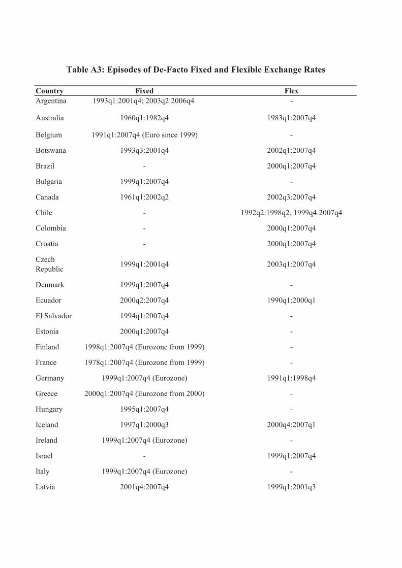
Country Fixed Flex

Argentina 1993q1:2001q4; 2003q2:2006q4 -

Australia 1960q1:1982q4 1983q1:2007q4

Belgium 1991q1:2007q4 (Euro since 1999) -

Botswana 1993q3:2001q4 2002q1:2007q4

Brazil - 2000q1:2007q4

Bulgaria 1999q1:2007q4 -

Canada 1961q1:2002q2 2002q3:2007q4

Chile - 1992q2:1998q2, 1999q4:2007q4

Colombia - 2000q1:2007q4

Croatia - 2000q1:2007q4

Czech

Republic1999q1:2001q4 2003q1:2007q4

Denmark 1999q1:2007q4 -

Ecuador 2000q2:2007q4 1990q1:2000q1

El Salvador 1994q1:2007q4 -

Estonia 2000q1:2007q4 -

Finland 1998q1:2007q4 (Eurozone from 1999) -

France 1978q1:2007q4 (Eurozone from 1999) -

Germany 1999q1:2007q4 (Eurozone) 1991q1:1998q4

Greece 2000q1:2007q4 (Eurozone from 2000) -

Hungary 1995q1:2007q4 -

Iceland 1997q1:2000q3 2000q4:2007q1

Ireland 1999q1:2007q4 (Eurozone) -

Israel - 1999q1:2007q4

Italy 1999q1:2007q4 (Eurozone) -

Latvia 2001q4:2007q4 1999q1:2001q3

Table A3: Episodes of De-Facto Fixed and Flexible Exchange Rates

Lithuania 1995q2:2007q4 -

Malaysia 1999q1:2007q4 -

Mexico - 1991q1:2007q4

Netherlands 1988q1:2007q4 (Eurozone from 1999) -

Norway - 1996q1:2007q4

Peru 1995q1:2007q4 -

Poland - 1999q1:2007q4

Portugal 1995q1:2007q4 (Eurozone) -

Romania - 1998q1:2007q4

Slovak

Republic1999q1:2007q4 -

Slovenia 1995q1:2007q4 -

South Africa - 1993q1:2007q4

Spain 2000q1:2007q4 (Eurozone) -

Sweden - 1993q1:2007q4

Thailand 1993q1:1997q2 1997q3:2007q4

Turkey - 1998q1:2007q4

United

Kingdom1960q1:1972q2 1972q3:2007q4

United States 1960q1:1971q3 1971q3:2007q4

Uruguay 1995q4:2001q4; 2005q3:2007q41988q1:1990q4; 1992q1:1995q3;

2002q1:2005q2

Total

Observations

1501 1119

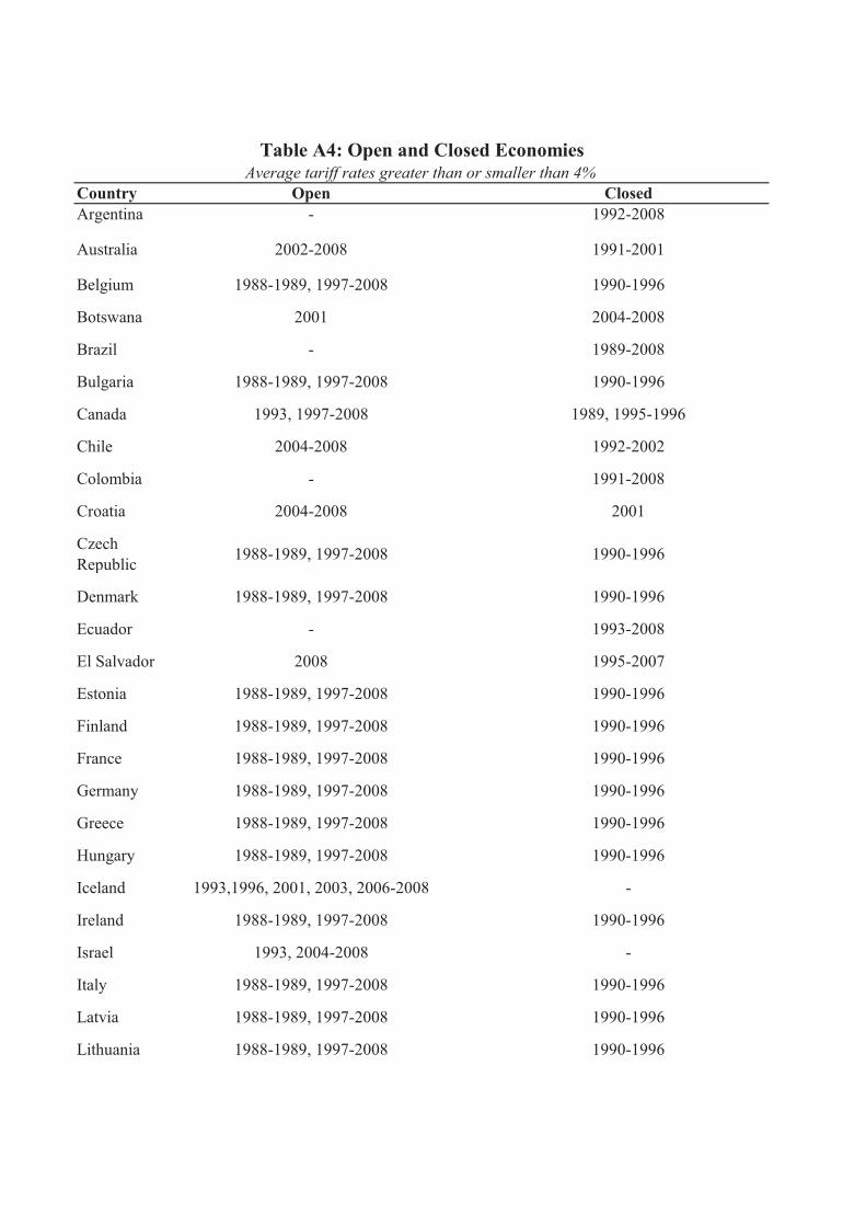
Country Open Closed

Argentina - 1992-2008

Australia 2002-2008 1991-2001

Belgium 1988-1989, 1997-2008 1990-1996

Botswana 2001 2004-2008

Brazil - 1989-2008

Bulgaria 1988-1989, 1997-2008 1990-1996

Canada 1993, 1997-2008 1989, 1995-1996

Chile 2004-2008 1992-2002

Colombia - 1991-2008

Croatia 2004-2008 2001

Czech

Republic1988-1989, 1997-2008 1990-1996

Denmark 1988-1989, 1997-2008 1990-1996

Ecuador - 1993-2008

El Salvador 2008 1995-2007

Estonia 1988-1989, 1997-2008 1990-1996

Finland 1988-1989, 1997-2008 1990-1996

France 1988-1989, 1997-2008 1990-1996

Germany 1988-1989, 1997-2008 1990-1996

Greece 1988-1989, 1997-2008 1990-1996

Hungary 1988-1989, 1997-2008 1990-1996

Iceland 1993,1996, 2001, 2003, 2006-2008 -

Ireland 1988-1989, 1997-2008 1990-1996

Israel 1993, 2004-2008 -

Italy 1988-1989, 1997-2008 1990-1996

Latvia 1988-1989, 1997-2008 1990-1996

Lithuania 1988-1989, 1997-2008 1990-1996

Table A4: Open and Closed EconomiesAverage tariff rates greater than or smaller than 4%

Malaysia 2006-2007 1988, 1991, 1993, 1996-1997,2001-2005

Mexico 2004-2008 1991, 1995, 1997-2003

Netherlands 1988-1989, 1997-2008 1990-1996

Norway 1988, 1993, 1996-2008 1995

Peru 2008 1993-2000, 2004-2007

Poland 1988-1989, 1997-2008 1990-1996

Portugal 1988-1989, 1997-2008 1990-1996

Romania 1988-1989, 1997-2008 1990-1996

Slovak

Republic1988-1989, 1997-2008 1990-1996

Slovenia 1988-1989, 1997-2008 1990-1996

South Africa - 1988-1993, 1996-2001, 2004-2008

Spain 1988-1989, 1997-2008 1990-1996

Sweden 1988-1989, 1997-2008 1990-1996

Thailand - 1989-1995, 2000-2006

Turkey 2003-2008 1993-1999

United

Kingdom1988-1989, 1997-2008 1990-1996

United States 1989-2008 -

Uruguay 2005-2008 1992, 1995-2004

Open Trade/GDP Closed Trade/GDP

Belgium 108.9% Argentina 19.4%

Bulgaria 112.3% Australia 33.2%

Botswana 100.0% Brazil 18.6%

Chile 64.2% Canada 54.8%

Croatia 87.4% Colombia 31.9%

Czech Republic 125.0% Ecuador 46.5%

Denmark 69.9% Finland 56.3%

El Salvador 63.3% France 40.8%

Estonia 154.7% Germany 59.9%

Hungary 79.4% Greece 42.0%

Iceland 74.4% Italy 41.3%

Ireland 118.0% Mexico 34.5%

Israel 80.8% Peru 36.3%

Latvia 98.6% Poland 52.9%

Lithuania 111.6% Romania 58.3%

Malaysia 132.5% South Africa 52.2%

Netherlands 217.1% Spain 37.8%

Norway 76.9% Turkey 42.7%

Portugal 60.1% United States 18.2%

Slovak

Republic141.5% Uruguay 37.9%

Slovenia 118.4%

Sweden 63.4%

Thailand 63.4%

United

Kingdom60.1%

Total

Observations1366 1234

Table A5: Open and Closed Economies(De-facto: Economies with a ratio of exports+imports to GDP greater than or less than 60%

Country High Debt Episodes

Argentina 2002-2006

Belgium 1981-2007

Brazil 1991-1993, 1999-2005

Bulgaria 1991-2001

Denmark 1983-1999

Ecuador 1990-1994, 1999-2000

Finland 1995-1997

Greece 1993-2007

Ireland 1981-1996

Israel 1996-2007

Italy 1982-2007

Malaysia 1990-1992

Netherlands 1992-1993

Poland 1992-1994

Portugal 1994-1996, 2003-2007

Sweden 1993-1999

Uruguay 2002-2006

Total

Observations1501

Table A6: Episodes of High Debt

(Gross Debt of Central Government Exceeding 60% of GDP)