HOUSTON GEOSPATIAL LEAD EXPOSURE … gratefully acknowledge the support and help of Kavitha Ganta,...
69
HOUSTON GEOSPATIAL LEAD EXPOSURE ANALYSIS: PRELIMINARY FINDINGS July 28, 2009 Winifred J. Hamilton, PhD, SM 1 , Brenda Reyes, MD, MPH 2 , Jyothi R. Domakonda 2 , Xuemei Wang, MS 3 , Richard D. DeBose, AICP 4 , Polly S. Ledvina, PhD, March 5 , Xia Li, MS 6 , Richard Dela Mater, BS 7 1 Environmental Health Section Chronic Disease Prevention and Control Research Center Department of Medicine Baylor College of Medicine Houston, TX 2 Bureau of Community & Children’s Environmental Health Houston Department of Health and Human Services Houston, TX 3 Division of Quantitative Sciences The University of Texas M.D. Anderson Cancer Center Houston, TX 4 Real Demand Consulting Houston, TX 5 PSL Integrated Solutions Houston, TX 6 Chronic Disease Prevention and Control Research Center Department of Medicine Baylor College of Medicine Houston, TX 7 Department of Health Disparities Research The University of Texas M.D. Anderson Cancer Center Houston, TX
Transcript of HOUSTON GEOSPATIAL LEAD EXPOSURE … gratefully acknowledge the support and help of Kavitha Ganta,...

HOUSTON GEOSPATIAL LEAD EXPOSURE ANALYSIS: PRELIMINARY FINDINGS
July 28, 2009
Winifred J. Hamilton, PhD, SM1, Brenda Reyes, MD, MPH2, Jyothi R. Domakonda2, Xuemei Wang, MS3, Richard D. DeBose, AICP4,
Polly S. Ledvina, PhD, March5, Xia Li, MS6, Richard Dela Mater, BS7
1Environmental Health Section Chronic Disease Prevention and Control Research Center
Department of Medicine Baylor College of Medicine
Houston, TX
2Bureau of Community & Children’s Environmental Health Houston Department of Health and Human Services
Houston, TX
3Division of Quantitative Sciences The University of Texas M.D. Anderson Cancer Center
Houston, TX
4Real Demand Consulting Houston, TX
5PSL Integrated Solutions
Houston, TX
6Chronic Disease Prevention and Control Research Center Department of Medicine
Baylor College of Medicine Houston, TX
7Department of Health Disparities Research
The University of Texas M.D. Anderson Cancer Center Houston, TX

Houston Geospatial Lead Exposure Analysis: Preliminary Findings 2
TABLE OF CONTENTS
TABLE OF CONTENTS.............................................................................................................................. 2PREFACE.................................................................................................................................................. 3ACKNOWLEDGEMENTS .......................................................................................................................... 4LIST OF TABLES....................................................................................................................................... 5LIST OF FIGURES..................................................................................................................................... 6APPENDICES ........................................................................................................................................... 8INTRODUCTION ....................................................................................................................................... 9
Health Effects of Lead Exposure ............................................................................................... 9Sources of Lead Exposure .......................................................................................................10Cost of Lead Exposure.............................................................................................................. 11
METHODOLOGY..................................................................................................................................... 11Cohort ........................................................................................................................................ 12Data ........................................................................................................................................... 12
City of Houston Department of Health and Human Services (HDHHS) .................................12
Harris County Appraisal District (HCAD)...................................................................................12
U.S. Census 2000 .....................................................................................................................12Data Evaluation and Cleaning .................................................................................................13Geospatial Addressing ............................................................................................................. 13Extracting Demographic Information ...................................................................................... 14Fitting the Parcel and Block Layers......................................................................................... 14The Biostatistical Model........................................................................................................... 15
RESULTS................................................................................................................................................ 17LIMITATIONS AND NEXT STEPS............................................................................................................ 19CONCLUSION......................................................................................................................................... 21REFERENCES ........................................................................................................................................ 22TABLES .................................................................................................................................................. 25FIGURES ................................................................................................................................................ 36APPENDICES ......................................................................................................................................... 50
Houston Geospatial Lead Exposure Analysis: Preliminary Findings 3
PREFACE
This report represents a preliminary analysis of the City of Houston Department of Health and Human Services Blood Lead Information and Management System (BLIMS) database, along with a number of housing and demographic risk factors.
The report focuses on the assessment of data sources, methodology, findings, limitations, and next steps identified that were associated with this analysis. This preliminary effort also included a number of necessary administrative components, including ethics and HIPAA training for new members of the research team, approval by Baylor College of Medicine’s Institutional Review Board (IRB) of the methodology and data protection procedures, establishment of sufficient and secure data storage space and procedures for the project, and execution of a Data Use Agreement between the City of Houston and Baylor College of Medicine. Overall time and funding constraints, along with these administrative issues, limited to some extent the time available to assess and analyze the blood-lead data and to evaluate alternative models and scenarios.
However, much preliminary work—including securing, assessing and cleaning the databases; geocoding blood-lead level data and numerous potential variables available at different spatial resolutions; and building two univariate and multivariate mixed-effects regression models—was completed. In addition, we were able to calculate—using the results of the parcel-level multivariate model—predicted blood-lead levels for 358,887 residential parcels in Houston and Harris County. Although these initial findings warrant additional scrutiny, we feel that our initial work and preliminary findings provide an excellent overview of the data and a useful platform for continued work.
July 2009

Houston Geospatial Lead Exposure Analysis: Preliminary Findings 4
ACKNOWLEDGEMENTS
We gratefully acknowledge the support and help of Kavitha Ganta, program analyst with the Houston Department of Health and Human Services (HDHHS), and Michele Austin, division manager in Contracts and Procurement at the HDHHS. This project had a very short timeline—approximately three months, and could not have been completed without their extra effort to help get a signed Data Use Agreement in place, as well as to assist with the data access and elucidation of the data structure, collection methodologies and underlying coding.
In addition to primary funding from the City of Houston for this project, funding support from the Houston Endowment Inc. was both necessary and appreciated. This project builds on a similar but smaller geospatial analysis of blood-lead data in Galveston, TX, which was funded by the Harris & Eliza Kempner Fund, with additional support from the Houston Endowment Inc. Without the methodology developed for the Galveston study, the current preliminary analysis could not have been accomplished within the relatively short time frame available for the analyses and report that follow.
The commitment and generosity of time and effort of all involved have been critical to what we hope will provide useful preliminary findings and that will lead to an extended collaboration to expand upon what is presented in this report. It is the hope and intent of the collaborators to utilize these and other data to enhance the lead-exposure and healthy-homes programs of the City of Houston, and thereby to also help improve public health and quality of life for area residents.
Houston Geospatial Lead Exposure Analysis: Preliminary Findings 5
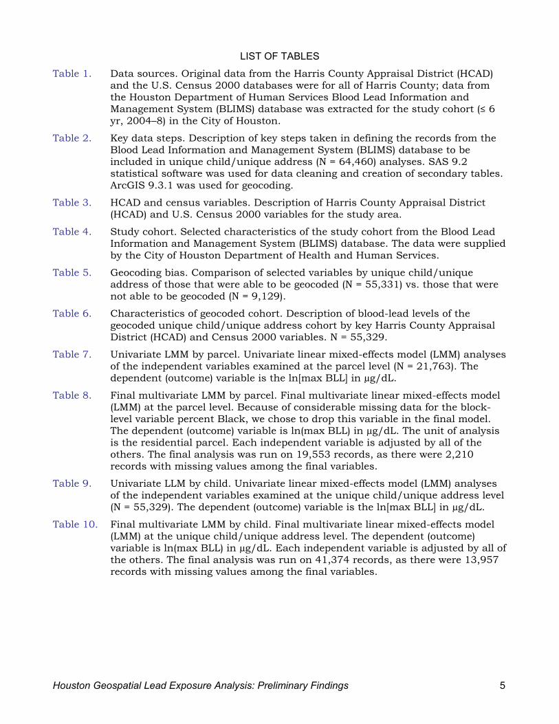
LIST OF TABLES
Table 1. Data sources. Original data from the Harris County Appraisal District (HCAD) and the U.S. Census 2000 databases were for all of Harris County; data from the Houston Department of Human Services Blood Lead Information and Management System (BLIMS) database was extracted for the study cohort (≤ 6 yr, 2004–8) in the City of Houston.
Table 2. Key data steps. Description of key steps taken in defining the records from the Blood Lead Information and Management System (BLIMS) database to be included in unique child/unique address (N = 64,460) analyses. SAS 9.2 statistical software was used for data cleaning and creation of secondary tables. ArcGIS 9.3.1 was used for geocoding.
Table 3. HCAD and census variables. Description of Harris County Appraisal District (HCAD) and U.S. Census 2000 variables for the study area.
Table 4. Study cohort. Selected characteristics of the study cohort from the Blood Lead Information and Management System (BLIMS) database. The data were supplied by the City of Houston Department of Health and Human Services.
Table 5. Geocoding bias. Comparison of selected variables by unique child/unique address of those that were able to be geocoded (N = 55,331) vs. those that were not able to be geocoded (N = 9,129).
Table 6. Characteristics of geocoded cohort. Description of blood-lead levels of the geocoded unique child/unique address cohort by key Harris County Appraisal District (HCAD) and Census 2000 variables. N = 55,329.
Table 7. Univariate LMM by parcel. Univariate linear mixed-effects model (LMM) analyses of the independent variables examined at the parcel level (N = 21,763). The dependent (outcome) variable is the ln[max BLL] in µg/dL.
Table 8. Final multivariate LMM by parcel. Final multivariate linear mixed-effects model (LMM) at the parcel level. Because of considerable missing data for the block-level variable percent Black, we chose to drop this variable in the final model. The dependent (outcome) variable is ln(max BLL) in µg/dL. The unit of analysis is the residential parcel. Each independent variable is adjusted by all of the others. The final analysis was run on 19,553 records, as there were 2,210 records with missing values among the final variables.
Table 9. Univariate LLM by child. Univariate linear mixed-effects model (LMM) analyses of the independent variables examined at the unique child/unique address level (N = 55,329). The dependent (outcome) variable is the ln[max BLL] in µg/dL.
Table 10. Final multivariate LMM by child. Final multivariate linear mixed-effects model (LMM) at the unique child/unique address level. The dependent (outcome) variable is ln(max BLL) in µg/dL. Each independent variable is adjusted by all of the others. The final analysis was run on 41,374 records, as there were 13,957 records with missing values among the final variables.
Houston Geospatial Lead Exposure Analysis: Preliminary Findings 6
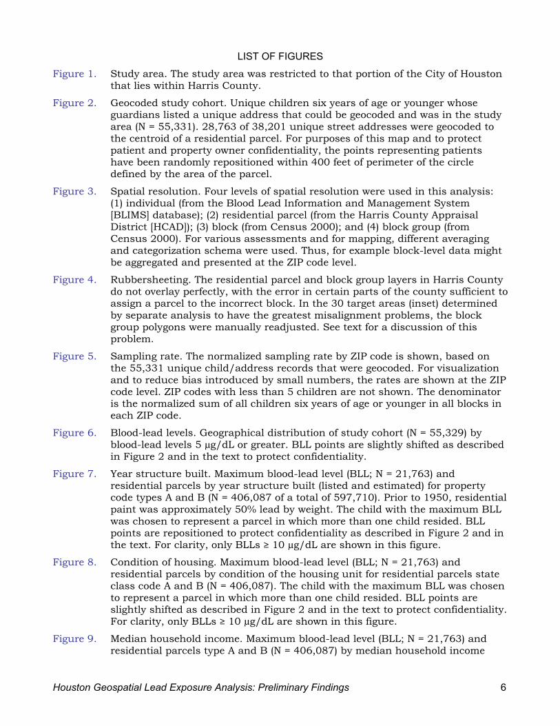
LIST OF FIGURES
Figure 1. Study area. The study area was restricted to that portion of the City of Houston that lies within Harris County.
Figure 2. Geocoded study cohort. Unique children six years of age or younger whose guardians listed a unique address that could be geocoded and was in the study area (N = 55,331). 28,763 of 38,201 unique street addresses were geocoded to the centroid of a residential parcel. For purposes of this map and to protect patient and property owner confidentiality, the points representing patients have been randomly repositioned within 400 feet of perimeter of the circle defined by the area of the parcel.
Figure 3. Spatial resolution. Four levels of spatial resolution were used in this analysis: (1) individual (from the Blood Lead Information and Management System [BLIMS] database); (2) residential parcel (from the Harris County Appraisal District [HCAD]); (3) block (from Census 2000); and (4) block group (from Census 2000). For various assessments and for mapping, different averaging and categorization schema were used. Thus, for example block-level data might be aggregated and presented at the ZIP code level.
Figure 4. Rubbersheeting. The residential parcel and block group layers in Harris County do not overlay perfectly, with the error in certain parts of the county sufficient to assign a parcel to the incorrect block. In the 30 target areas (inset) determined by separate analysis to have the greatest misalignment problems, the block group polygons were manually readjusted. See text for a discussion of this problem.
Figure 5. Sampling rate. The normalized sampling rate by ZIP code is shown, based on the 55,331 unique child/address records that were geocoded. For visualization and to reduce bias introduced by small numbers, the rates are shown at the ZIP code level. ZIP codes with less than 5 children are not shown. The denominator is the normalized sum of all children six years of age or younger in all blocks in each ZIP code.
Figure 6. Blood-lead levels. Geographical distribution of study cohort (N = 55,329) by blood-lead levels 5 µg/dL or greater. BLL points are slightly shifted as described in Figure 2 and in the text to protect confidentiality.
Figure 7. Year structure built. Maximum blood-lead level (BLL; N = 21,763) and residential parcels by year structure built (listed and estimated) for property code types A and B (N = 406,087 of a total of 597,710). Prior to 1950, residential paint was approximately 50% lead by weight. The child with the maximum BLL was chosen to represent a parcel in which more than one child resided. BLL points are repositioned to protect confidentiality as described in Figure 2 and in the text. For clarity, only BLLs ≥ 10 µg/dL are shown in this figure.
Figure 8. Condition of housing. Maximum blood-lead level (BLL; N = 21,763) and residential parcels by condition of the housing unit for residential parcels state class code A and B (N = 406,087). The child with the maximum BLL was chosen to represent a parcel in which more than one child resided. BLL points are slightly shifted as described in Figure 2 and in the text to protect confidentiality. For clarity, only BLLs ≥ 10 µg/dL are shown in this figure.
Figure 9. Median household income. Maximum blood-lead level (BLL; N = 21,763) and residential parcels type A and B (N = 406,087) by median household income

Houston Geospatial Lead Exposure Analysis: Preliminary Findings 7
(block group; N = 1,159). The child with the maximum BLL was chosen to represent a parcel in which more than one child resided. BLL points are slightly shifted as described in Figure 2 and in the text to protect confidentiality. For clarity, only BLLs ≥ 10 µg/dL are shown in this figure.
Figure 10. Percent Hispanic/Latino. Maximum blood-lead level (BLL; N = 21,763) and residential parcels state class code A and B (N = 406,087) by percent Hispanic/Latino (block; N = 8,086 of 9,222). The child with the maximum BLL was chosen to represent a parcel in which more than one child resided. BLL points are slightly shifted as described in Figure 2 and in the text to protect confidentiality. For clarity, only BLLs ≥ 10 µg/dL are shown.
Figure 11. Education. Maximum blood-lead level (BLL; N = 21,763) and residential parcels type A and B (N = 406,087) by percent of individuals 25 years or older with some college (block; N = 1,158 of 1,159). The child with the maximum BLL was chosen to represent a parcel in which more than one child resided. BLL points are slightly shifted as described in Figure 2 and in the text to protect confidentiality. For clarity, only BLLs ≥ 10 µg/dL are shown in this figure.
Figure 12. Predicted blood-lead levels by parcel. Predicted blood-lead levels (BLLs) in children 2 to 3 years of age in all class A and B residential parcels in the study area for which there was complete information (N = 358,887 of 406,087 state class code A or B of total 597,710 parcels) calculated from the final multivariate linear mixed-effect model (LMM) at the parcel level (Table 8), with percent Black by block excluded (see text) Actual BLLs (offset as described in Figure 2 and in the text to protect confidentiality), by parcel, are also shown; for visual clarity only BLLs ≥ 10 µg/dL are shown on this figure.
Figure 13. Autocorrelation. Analysis of residual clustering using the local Moran’s I statistic (LM), a “decomposition” of the global Moran’s I statistic. The LM is a measure of the degree to which model results are affected by missing spatial variables. The residuals from the final multivariate linear mixed-effects model (LMM) at the parcel level (N = 19,553; Table 8) were used. For this analysis, an effective search radius of approximately 6,065 feet was used around each parcel centroid. Groups of statistically significant clusters of high residual values (red dots) are indicative of areas for which the model most likely underpredicts, whereas groups of statistically significant low residual values (yellow dots) are indicative of areas for which missing the model most overpredicts. The global P-value is 0.01, suggesting that additional variables may need to be included in the model. Approximately 600 observations are poorly predicted by the model, and many of these outliers are geographically clustered. This may be useful in determining additional variables for inclusion in the model.

Houston Geospatial Lead Exposure Analysis: Preliminary Findings 8
APPENDICES
Appendix 1H. Abbreviations
HHAppendix 2.H SAS script (version 9.2; SAS Institute Inc., Cary, NC) for the key data examinations and univariate and multivariate models.

Houston Geospatial Lead Exposure Analysis: Preliminary Findings 9
INTRODUCTION
The purpose of this analysis is to better understand lead exposure in Houston, Texas, and to help guide future remediation efforts. In addition, the City of Houston’s Department of Health and Human Services (HDHHS) maintains a particularly rich dataset on lead exposure and risk factors, and the Harris County Appraisal District maintains one of the most comprehensive housing databases in the U.S. Analyses of these resources may prove useful to the Houston community, as well as to other communities lacking such data.
A comprehensive discussion of lead exposure is beyond the scope of these limited, preliminary analyses of lead-exposure and risk factors in Houston, Texas. Several excellent reviews and resources are available (1,12,14,23,36), although ongoing research continues to elucidate the damage and mechanisms of harm associated with lead exposure. The following very briefly reviews the health effects, sources and cost of lead exposure.
Health Effects of Lead Exposure
Early exposure to lead results in persistent reductions in cognitive ability and increases in behavioral problems. In addition, early exposure is increasingly linked to adult health problems later in life, including cardiovascular and neurodegenerative disease and early mortality (12,16,22,29,35,38,40,43). Although a blood-lead level (BLL) of 10 µg/dL is used by many public health departments as an “action level,” the CDC and lead experts around the world are unequivocal in stating that there is no safe level of lead in the human body. Indeed, recent research indicates that the negative effects of lead on a child’s intelligence and social behavior are not linear, i.e., the damage does not correlate strictly with dose. Instead, studies are consistently demonstrating that the damage per given dose is measurably greater below 10 µg/dL than above (3,20). For example, Canfield and associates found a decrease of 7.4 IQ points in children as BLLs increased from 1 to 10 µg/dL and a more gradual decrease in IQ of 2.5 points as BLLs increased from 10 to 30 µg/dL (3).
Concomitant with the realization that tiny amounts of lead do irreparable harm to young children is a growing body of evidence linking early exposure to lifelong health problems. We know now that much of the lead to which one is exposed is stored in the body, generally in bone, and this lead can continue to damage health throughout life. Levels of lead in bone in adults have now been linked to hypertension, cardiovascular disease, premature death, problems with fertility, and immune and neurodegenerative disorders (12,16,22,29,34,35,38,40,43). Although the focus of this report is primarily on children, lead exposure in children and in adults is inextricably linked. One particular area of intense interest is fetal exposure. During pregnancy, even if a woman is not being exposed to lead in her home or workplace, lead leaching from her own bones from past exposures can expose her fetus to deleterious amounts of lead at a critical time in her yet-to-be-born child’s neurodevelopment.
Some of the mechanisms by which lead appears to damage normal biologic mechanisms include substitution of lead for other essential metals, especially calcium and zinc; alteration of the structure and function of metal-binding proteins; inhibition of key enzymes necessary for the synthesis of heme which is, in turn, important for proper red blood cell formation and for regulating metabolism; interference with proper DNA binding and gene expression by destabilizing the zinc-finger domains necessary for the proper shape of DNA; disruption of neural transmission by altering calcium transport; and promotion of damaging reactive oxygen species within blood vessels, a key mechanism underlying lead-associated hypertension and cardiovascular disease. Considerable current research is directed at better understanding the mechanisms by which lead and other heavy metals damage health.
Houston Geospatial Lead Exposure Analysis: Preliminary Findings 10
Sources of Lead Exposure
In the U.S. today, ingestion is the most common route of lead absorption. Before lead in most gasoline was finally eliminated in the U.S. in 1996, inhalation was a major source of exposure. Deteriorating house paint is the largest single source of lead exposure and the major source of lead poisoning in children (33). Housing built before 1950, which makes up 22.3% of the U.S. housing stock, poses the greatest risk because house paint contained the highest amount of lead (up to 50% by weight) prior to this time. Renovation of older residential buildings without taking proper precautions can result in not only poisoning the workers and residents but can seriously contaminate the home and the area around the home or apartment. Although the use of lead-based household paint in the U.S. was banned in 1978, lead-based paint continues to be used for numerous industrial uses, such as on marine vessels and bridges.
Other common sources of exposure include soil and water. Lead adheres tenaciously to soil particles and thus lead contamination from car exhaust, paint dust and lead-based pesticides persists for decades. Soil may be contaminated around older wooden homes with exterior lead paint, especially following improper power sanding to prepare the exterior for painting (15), which can release significant amounts of lead dust. The U.S. EPA considers a soil-lead level of 400 ppm in a play area to be a hazard. Sixteen percent of pre-1980 homes have adjacent soil lead concentrations > 500 ppm, and the chance of having levels > 500 ppm is 4–5 times higher if the house has exterior lead-based paint. Indeed, lead in urban soil is increasingly regarded as a potentially major source of lead poisoning, especially among children (25,44), and even in lead-safe homes and schools significant levels of lead can often be found near entrances where lead is tracked in from outdoors (21). Also, soil along freeways or older roadways is generally contaminated by past emissions of lead in auto exhaust, with the levels decreasing with distance from the roadway and proportionate to traffic volume (11). The Agency for Toxic Substances and Disease Registry (ATSDR) estimates that leaded gasoline use left behind 4 to 5 million metric tons of lead in the environment (44).
Lead is rarely found in source water, but enters tap water through corrosion of plumbing materials. Exposure to lead from contaminated tap water is a significant source of body burden in many communities, and can vary from household to household based on the type of plumbing and fixtures. The U.S. Environmental Protection (EPA) estimated in 1991 that 14% to 20% of the total U.S. lead exposure was from drinking water (24). In most instances the sources are lead pipes, plumbing fixtures and solder along distribution lines.
Other sources of lead exposure include lead-glazed pottery and dishes, leaded crystal, various Mexican chile and tamarind candies, folk remedies such as greta and azarcón (4), cosmetics such as the eye liner kohl (32), some hair dyes, and hobbies such as recreational shooting with powder charges (39).
In addition, an estimated 95% of elevated BLLs in adults are attributable to occupational exposure (5,6), with approximately 0.5 and 1.5 million workers exposed to lead in the workplace (1). Industries that expose workers to lead include battery manufacturing, painting, rubber products and plastics industries, municipal waste incineration, soldering, steel welding and cutting operations, lead compound manufacturing, nonferrous smelting, radiator repair, brass and bronze foundries, pottery production, scrap metal recycling, firing ranges, and wrecking and demolition. Approximately 2–3% of children with a BLL ≥10 µg/dL have been exposed to “take-home” lead, that is, lead brought home from the workplace on the clothes or in the vehicles of their adult caregivers.
Because lead is stored in bone, lead can be released back into the blood and become a source of exposure as bone undergoes remodeling or in certain disease states. Fetuses and
Houston Geospatial Lead Exposure Analysis: Preliminary Findings 11
young children can also be exposed to maternal blood lead and to lead during breast feeding. Transfusion in neonates is another exposure pathway, as is contact with lead-containing products such as vinyl lunch boxes, jewelry and artificial turf.
Several new regulations, including a 2008 rule issued by the EPA that requires contractors performing renovation, repair and painting projects that disturb lead-based paint in homes, child care facilities, and schools built before 1978 to be certified and to follow specific work practices to prevent lead contamination, should help to reduce exposure. This rule becomes effective in April 2010 (42). In addition, the Consumer Product Safety Commission recently issued a rule that phases out the amount of allowable lead in children’s products such as toys and books from 600 ppb in 2008 to 100 ppb in 2011 (41).
The effective dose and short- and long-term effects are modulated by not only exposure, but also by numerous yet poorly understood variables including age, timing of exposure, ethnicity, health status, behavior, nutrition, psychosocial stress and education (10).
Cost of Lead Exposure
Lead neurotoxicity does not only decrease IQ, but also decreases graduation rates and increases antisocial and criminal behavior. Lead is linked with numerous behavior disorders and learning problems including dyslexia, autism, attention deficit disorder, diminished self esteem, and increased aggression and impulsivity. Rick Nevin, an economist and consultant for the Center for Healthy Housing, examined the temporal relationships between the rates for multiple types of crime and the amount of lead in gasoline and paint lead (30). Using a lag of approximately 20 years, he demonstrated that since the early 1900s, the rates of virtually all types of major crime in the U.S. have followed remarkably closely to the changes in lead exposure, suggesting a strong influence of lead exposure on criminal activity (30). Nevin has also analyzed lead and scholastic achievement in the U.S. and found that 1936–1990 preschool BLL trends explained 45% and 65% of the 1953–2003 variation in average scholastic achievement test (SAT) verbal and math scores, respectively (31).
Because of the number of people affected and the lifetime legacy of early exposure to lead, the human, social, public health and economic burden in the U.S. is immense (1,2,8,9,12,17-19,37). Landrigan and associates at Mount Sinai School of Medicine, for example, conservatively estimate that the annual cost in the U.S. attributable to childhood lead poisoning is $43.5 billion (18). They note that this does not include pain and suffering or diseases of adulthood, such as hypertension or premature mortality, linked to childhood exposure to lead (28).
Our analysis is intended to increase our understanding of lead exposure in the Houston area, and to provide a flexible geospatial and statistical model that can be subsequently refined to address additional risk factors and to better understand the short- and long-term efficacy of various interventions.
METHODOLOGY
The objective of the geospatial analysis was to use available data on BLLs of children, housing and demographics to develop a multivariate statistical model to predict residential housing units most likely to be associated with elevated blood-lead levels and that would be useful to the HDHHS and the Houston community in general for reducing lead exposure.
Because the study involved patient data, we first received Baylor College of Medicine Institutional Review Board (IRB) approval of our methodology, as well as a fully executed Data Use Agreement between the City of Houston and Baylor College of Medicine. These documents detail the methods used to safeguard and protect the confidentiality of the data.

Houston Geospatial Lead Exposure Analysis: Preliminary Findings 12
The following sections of the Methodology describe the cohort, data sources, geospatial techniques and statistical approaches used in this analysis.
COHORT
The cohort included all children 6 years of age or younger from whom one or more valid BLL measurement(s) were obtained between January 1, 2004.and December 31, 2008, and whose guardians listed a residential address within the City of Houston and within Harris County. The study area is shown in Figure 1.
DATA
City of Houston Department of Health and Human Services (HDHHS) The Bureau of Community and Children’s Environmental Health maintains the Blood Lead Information and Management System (BLIMS), an Oracle-based data collection system that consists of twelve linked tables. The BLIMS stores BLL measurement data, demographic and behavioral information, data collected as part of environmental assessments and other relevant data. The BLIMS collects BLL data from multiple sources for submission to the State of Texas Child Lead Registry and/or the Texas Systematic Tracking of Elevated Lead Levels and Remediation (STELLAR) database. STELLAR is a software application developed by the CDC and provided free of charge to state and local Childhood Lead Poisoning Prevention Programs (CLPPPs) to help track lead poisoning cases (7). The HDHHS BLIMS database includes all data necessary to reporting to STELLAR, as well as additional information used in the HOUSTON CLPPP program and, to a lesser extent, its healthy homes programs. The team utilized for this study four of the twelve tables in BLIMS: address, child, lab and provider. For this analysis and for each of the four tables, we utilized those records from the HDHHS that resulted from a query to select children six years of age or younger from whom was obtained a BLL between January 1, 2004 and December 31, 2008. Table 1 lists the BLIMS tables, received as an Access 2003 database, and fields used for this preliminary analysis. Table 2 chronologs the key steps taken in assessing, cleaning and preparing for analysis the BLIMS data. Note that the BLIMS database contains a unique address identifier that is at a finer resolution than the street or parcel address. This level of resolution allowed us to examine not only BLLs and risk factors at different street addresses, i.e., residential tax parcels, but also to examine these variables in different residential units (e.g., apartments) within the same tax parcel.
Harris County Appraisal District (HCAD) Tax appraisal records and associated shapefiles for 1,345,024 Harris County parcels were downloaded from http://pdata.hcad.org, along with available data dictionaries. Three appraisal data tables from the Access database were used in this analysis, as listed in Table 1. Key fields utilized in the analysis included address, date erected, improvement value (structure only), state class property code (e.g., A1 = single family residential, B1 = multifamily residential), condition of structure, and heated (livable) area. We also examined a number of other fields, including building type and style codes, which were useful on occasion for understanding certain state class property codes. Using geospatial methods to reduce the database to just those parcels within the City of Houston and Harris County resulted in a total of 597,710 parcels (Table 3).
U.S. Census 2000 We used U.S. Census 2000 information for two different geographic scales: block and block group (Table 1). U.S. Census 2000 information is available from http://factfinder.census.gov. In general, block data are from Summary Files 1 (SF1) and represent actual count data, whereas block-group data are from SF3 data, which are a

Houston Geospatial Lead Exposure Analysis: Preliminary Findings 13
sample of 1 in 6 individuals extrapolated for the entire population. SF1 data included in the analysis were population, ethnicity by race, sex, age, and owner or renter occupied. In the study area there were 9,222 census blocks. SF3 data included in the analysis were educational attainment, median household income, and median year structure built. In our study area, there were 1,159 block groups. Table 3 provides an overview of the census data utilized.
DATA EVALUATION AND CLEANING
We used ArcMap and SAS in tandem to assess, clean, limit to the study area, merge and categorize the data for subsequent geospatial and statistical work. Table 2 provides an overview of steps taken to assess and prepare the BLIMS database. After limiting the BLL records to inclusion criteria, there were 119,221 unique BLL records (includes multiple measurements on the same child), 64,460 unique children at unique addresses (in this cohort no child had BLL measurements taken at different addresses; 3 of the 64,460 children had no BLL listed), 4,904 unique addresses with more than one child (e.g., siblings), and 38,201 unique street addresses. Selected characteristics of the cleaned BLIMS databases are shown in Table 4. Note, in Tables 3 and 4, that there were variable amounts of missing data in the three databases. Evaluation of the data quality, completeness and relevance for the analysis determined selection of some of the fields and categorization schema for the subsequent analyses.
GEOSPATIAL ADDRESSING
The map projection used was NAD83, Texas South Central Zone, State Plane, feet. For purposes of this analysis, for which the level of analysis is primarily the parcel, BLIMS street addresses were matched to HCAD addresses, which then linked each geoaddressed child to an HCAD parcel account number. Of the 38,201 unique street addresses, we were able to geoaddress 31,819 (83.3%). However, 621 of these were in Houston but not Harris County, and 3,776 were not in Harris County; therefore these 4,397 did not meet our inclusion criteria and were removed. Of the 27,422 that geocoded in Houston and Harris County, our SAS assessment determined that 5,659 did not meet other inclusion criteria (age or study period). Thus, of the geoaddressed unique street addresses, 21,763 geocoded to an HCAD parcel address and met the study’s inclusion criteria. Of the 64,460 unique children/unique address records that met the inclusion criteria, we were able to geoaddress 55,331 (85.8%; Figure 2). This includes some children at the same street address (i.e., multiple children at unique address identifiers and multiple unique address identifiers at the same street address).
For those addresses that could not be adequately geocoded by matching to an HCAD parcel address and/or using ArcGIS’s address locator with or without simple adjustments (e.g., correction of a simple misspelling of a street name or correcting a wrong ZIP code) to link to a parcel, we utilized the Southeast Texas Addressing and Referencing Map (STAR*Map, version 4.0, 2006; www.h-gac.com/rds/gis/starmap), which is maintained by the Houston-Galveston Area Council; online address locators (e.g., Google Maps, Yahoo Maps and MapQuest), and U.S. postal databases to help resolve addressing problems when possible and within the time constraints of the project. Among the reasons we identified that limited our ability to geoaddress records included (1) only a P.O. Box provided, (2) address could not be matched to a parcel address, and (3) incorrect or incomplete address information that could not be resolved. Each satisfactorily geocoded record was assigned xy coordinates within the map projection and coordinate system used. All changes or problems with addresses were coded and recorded.
A comparison of the two groups (geoaddressed = 55,331 vs. not geoaddressed = 9,129; Table 5) at the unique child/unique address level (BLIMS data) demonstrated no significant
Houston Geospatial Lead Exposure Analysis: Preliminary Findings 14
differences in gender or age between the two groups. However, the two groups were significantly different with regard to race/ethnicity and mean and median BLLs. With regard to race/ethnicity more Hispanic/Latino children geocoded than did not, and more children in the Other category did not geocode. In the BLIMS database, there are an unusually large number of children in the Other category, most of whom were coded as Unknown, which was thought to be the result in part in changes in coding instructions for race and ethnicity over time. Some of the bias observed for this variable may relate to temporal/spatial differences (different neighborhoods tend to be targeted for surveillance) introduced in coding. In addition, the mean BLL was higher in the geocoded group (3.1 vs. 3.0 µg/dL) with a larger range of values in the geocoded group. This may have been driven in part by several outliers (e.g., 326 µg/dL) in the geocoded group, but it is also reasonable to think that addresses are more likely to be resolved in children with higher BLLs as these children often require follow-up assessments.
EXTRACTING DEMOGRAPHIC INFORMATION
Our model included four levels of spatial information (Tables 3 and 4; Figure 3) that could be used to characterize the unique child/unique address or parcel records: (1) individual child information (e.g., BLL, age, and gender) from the BLIMS database; (2) parcel information (e.g., age built, type of property, and improvement value) from the HCAD database; (3) Census 2000 block information (e.g., population, race, ethnicity); and (4) Census 2000 block group information (e.g., median household income, education, median year built of housing in block group). Each of the 55,329 children with one or more BLL measurements and each of the 21,763 residential parcels were characterized by the best available information that were likely to be important variables to be included in the multivariate and predictive models. For this analysis, models were built at both the unique child/unique address and at the parcel levels, with the parcel-level model used to calculate the predicted BLLs by residential parcel. Mean, 90th percentile, and maximum BLLs were explored for representing multiple BLL readings in the same child and for characterizing parcels with multiple children. For our analyses, we chose to use maximum BLLs (see also “The Biostatistical Model”).
FITTING THE PARCEL AND BLOCK LAYERS
The HCAD parcel and census block layers do not line up precisely, with greater misalignment in certain areas than others. This is an acknowledged problem with U.S. Census 2000 data, which is generally not quite as accurate as more locally generated and maintained digital maps (such as STAR*Map) and tax appraisal parcel data. After verifying the projections, we consulted with Houston-Galveston Area Council, the maker of the STAR*Map and were informed that the slight misalignment was due to the fact that the local maps had been refined using aerial photography but the census map had not. For Census 2010 it is anticipated that much of this problem will be resolved as Census volunteers will be collecting GPS coordinates along with survey data. Although it is possible to use a technique called “rubbersheeting” to manually manipulate census-block polygons features so that their boundaries line up reasonably well with the HCAD parcel line features, in reality and given the size of Harris County and time constraints, this was not reasonable. To maximize the percentage of parcels accurately assigned to a Census block, we did the following.
First, each parcel was spatially defined by its centroid, a single point in the center of the parcel as calculated by the area and shape of the parcel polygon. Then each of the 597,710 parcels was assigned to the block in which its centroid fell. In most instances, even with some misalignment, this resulted in the correct assignment. Second, we developed a macro that analyzed Harris County for areas in which the block-group boundaries intersected with

Houston Geospatial Lead Exposure Analysis: Preliminary Findings 15
the greatest number of parcel boundaries. This identified 30 areas of particular concern (Figure 4). For these 30 areas, which tended to be in the outer less densely developed and/or rapidly developing areas, the block-group boundaries were manually adjusted (Figure 4). After spatial adjustment, a separate analysis estimated that approximately 3% of the parcels in the study area might be assigned to the wrong block; it is unlikely that any would be assigned to the wrong block group. Even in instances in which a parcel was assigned to the wrong group, it is unlikely that such assignment would have much of an effect as (1) adjacent blocks generally have similar characteristics, (2) the block-group variables would still be accurate, (3) the suspect areas tend to be in newer and/or sparsely populated areas where elevated predicted BLLs are unlikely, and (4) the large number of residential parcels in the predictive model. Nevertheless, this is an area for future improvement.
Selected characteristics of the 55,331 geoaddressed children, by BLL, are shown in Table 6. As noted earlier, mapping was used in tandem with the statistical explorations to help understand the data. Figure 5 reflects the age-adjusted sampling rate for children 6 years of age or younger, aggregated by ZIP code. In Figure 6, the geocoded BLLs are shown (for clarity, because of the large number of observations, only BLLs ≥ 5 µg/dL are shown).
Note that, in all the maps included with this report in which an individual point representing a BLL is shown, the point has been randomly shifted to protect the confidentiality of the child and his or her family, as well as the property owner. We developed an algorithm for this process that takes into account the size of the parcel. Thus, for each of the BLL observations, which were mapped to the centroid of the appropriate parcel, we overlaid on the centroid a circle based on the area of the parcel polygon and then randomly positioned the BLL observation between 0 and 400 feet from a random position along the perimeter of the circle. This random shift paradigm maintains the spatial distribution of the blood-lead data while at the same time making it impossible to visually link a BLL measurement with a parcel or street address. The shifted points are only used for visualization.
THE BIOSTATISTICAL MODEL
We used ArcGIS 9.3.1 (ESRI, Redlands, CA) to overlay the spatial data, create maps and generate merged databases for statistical analysis. SAS 9.2 (SAS Institute, Cary, NC) was used to explore the original datasets, clean the data, create secondary .dbf databases for geospatial analysis and mapping, and develop the univariate and multivariate linear mixed-effects models (LMMs). As noted earlier and selectively displayed in Tables 1-6, descriptive statistics were used to examine all of the databases and the variables included in the maps and in building the models. The complete SAS script is included in Appendix 2.
We chose to use the highest BLL of each child for the unique child/unique address model (maximal N = 55,329), since the health effects from lead are thought to be largely irreversible and the highest measured level may more accurately reflect the potential health consequences the individual might experience. This approach has also been used in other previous studies (26). For the parcel analysis (maximal N = 21,763), for those 4,904 parcels with more than one child, we chose the child with the maximal BLL (which was equal to choosing the child at the 90th %tile) as representative of the parcel. For 4,294 of the 4,904 parcels, two children resided in the same parcel.
As noted earlier, because we had address data at a higher resolution than street address but also were committed to building a predictive model at the parcel level, we chose to build two models: (1) parcel level, and (2) unique child/unique address level.
Note that, of 597,710 parcels in the study area, information on year erected was available

Houston Geospatial Lead Exposure Analysis: Preliminary Findings 16
for 469,603 (Table 3). Because of the importance of building age in predicting lead poisoning and because records with missing data must be dropped from the regression model, we developed a multivariate linear regression model that was used to estimate the year built of each building type using key variables, including improvement value, property state class code and the median year built of structures in the block group, as covariates. The general equation used to estimate year built for the missing records, by building type (A, B or Other), is shown below.
Year BuiltPredicted = Estimate + Intercept + (Coefficient x Improvement Value) +
(Coefficient x Median Year BuiltBlockGroup)
Because the BLLs were not normally distributed, they were ln-transformed. The dependent (outcome) variable was ln[max BLL] for both models. The independent (predictor) variables examined included gender, individual-level race/ethnicity, age (four categories), building type (three categories), improvement value (per square foot of living area), year residential structure built (actual plus predicted), condition of residential structure, population by block, percent owner occupied by block, median year built by block group, percent with some college by block group, and median household income by block group.
We conducted all univariate and multivariate analyses of predictors of ln[max BLL] using a LMM. The two final multivariate models were built using a backward elimination technique, initially including all of the independent variables that were found to be significant in the univariate analyses and then removing each nonsignificant variable, one at a time, and rerunning the model until only significant variables remained. The final parcel and unique child/unique address models included 19,553 (2,210 missing) and 41,374 (13,957 missing) observations, respectively. For the parcel model, we built the model both with and without percent Black by block, choosing to use the model for the predictive model that excluded percent Black by block as there were considerable missing census data (8,454 missing) for the model when the variable percent Black was included.
The regression residuals from the final parcel LMM were examined for spatial autocorrelation (clustering) using Moran’s I global and local statistics to help assess model performance. Moran’s I is a measure of the probability that adjacent observations (in this instance, the residuals) are correlated. A “0” score equals random dispersion, whereas values that approach -1 or +1 indicate clustering, i.e., patterns that adjusting for the variables in the final model did not remove. The local Moran’s (LM) statistic is in effect a decomposition of the global Moran’s I statistic and was used to help define geographic areas where remaining spatial autocorrelation may be a problem. For our analysis, an effective search radius of approximately 6,065 feet was used around each parcel centroid. High LM values indicate positive spatial autocorrelation, i.e., clusters of either similarly high or similarly low data values. Each LM value has an associated Z-score and P-value, indicators of the likelihood that a particular cluster appears by chance.
From the final model on the parcel level, the coefficients of the predictor variables were used to calibrate the relative weights assigned to each of the risk factors in each parcel, by age and by building type (A or B) and to compute an estimated ln[max BLL] for each residential tax parcel in the study area for which there was complete information on the variables in the final model (N = 358,887 for the model in which percent Black excluded; N = 242,530 for the model in which percent Black included). The general equation used to predict the BLLs for the highest risk age group, 2-3 years of age, based on the parcel multivariate model that excluded percent Black by block, follows. A separate multivariate regression model was also fit that included percent Black by block. Year built includes actual and predicted values. The predictions were run just for building types (state class codes) A (generally houses) and B (generally apartments) as “Other” was extremely diverse. The general equation for the

Houston Geospatial Lead Exposure Analysis: Preliminary Findings 17
predicted BLLs is shown below.
Ln[maxBLL]Predicted = 1.1214 + 0.1881 + (-0.1772 x Building Type = A) + (0.1782 x Building
Type = B) + (0.1004 x Year Built ≤ 1950) + (0.0594 x Year Built >1950 to ≤1978) + (0.0147 x
Total PopulationBlock) + (0.0012 x Percent Hispanic/LatinoBlock) + (-0.0055 x Median Household
IncomeBlockGroup)
RESULTS
Characteristics of the study population (N = 64,460 of which 3 did not have a BLL and 55,329 with BLLs geocoded) and variables by BLLs are summarized in Tables 4–6. The mean BLL in the study cohort (N = 64,457) was 3.1 µg/dL, with a range of 0 to 326 µg/dL. Children between 2 and 3 years of age displayed the highest mean BLL (3.3 µg/dL); children between 6 and 7 years of age had the lowest mean BLL (2.7 g/dL). The majority of the children lived in property type A1 (a single-family residential home; N = 23,320) or in B1 (a multifamily residence such as an apartment complex; N = 22,685). Children who lived in A1 housing had a higher mean BLL than those who lived in B1 housing (3.3 and 2.9 µg/dL, respectively). The BLLs of children who lived in housing built in 1950 or earlier were significantly higher (3.6 µg/dL) compared with those who lived in housing built between 1951 and 1978 (2.0 µg/dL) or after 1978 (2.9 µg/dL). The HCAD-rated condition of the residence tracked linearly with mean BLLs, with children living in structures rated as poor having a mean BLL of 3.9 µg/dl, whereas those living in housing rated as excellent had a mean BLL or 2.5 µg/dL. More than half of the cohort (67.4%) lived in housing rated average, fair or poor. This may reflect in part higher surveillance in neighborhoods and populations thought to be at higher risk. Among those children who were geocoded (Table 6), similar trends were observed, with 2–3 year-old children, those living in homes built in or before 1950, and those living in single-family homes generally having higher BLLs. In general, children who lived in state class codes B2, B3 and B4 (two– to four–family residences) tended to have the highest mean BLLs (3.7 µg/dL). Note, however, that the only a small percentage (approximately 5%) of the study cohort that lived in code B housing lived in B2–4 housing (95% lived in B1 housing), and that B2–B4 housing is diverse and use of additional building style codes suggests that these classes may include some single-family homes. Additional exploration of these codes and of potential relationships between residential building types and BLLs is warranted.
We also used mapping to explore and visualize the data. The 55,331 addresses of the unique children at unique addresses we were able to geocode are shown in Figure 2, with BLLs ≥ 5 µg/dL shown in Figure 6. Figures 7 though 11 show various HCAD and Census 2000 variables, including year structure built (Figure 7), condition of residential structure (Figure 8), median household income by block group (Figure 9), percent Hispanic/Latino by block (Figure 10), and percent of adults with some college by block group (Figure 11), that may be associated with elevated BLLs. For each of these figures, we have overlaid the distribution of BLL observations ≥ 10 µg/dL.
The results of the parcel-level (maximum 21,763 records if no missing variable data) and unique child/unique address-level (maximum 55,329 records if no missing variable data) univariate analyses are shown in Tables 7 and 9, respectively. In the parcel exploration of the individual independent variables using the LMM, all of the variables except gender P = 0.50), percent Black by block (P = 0.69), and living in a home built after 1978 (P = 0.22) were individually significant predictors of BLLs. Among the categorical variables, elevated BLLs were associated with living in type B housing (compared with Other), being 2–3 years of age

Houston Geospatial Lead Exposure Analysis: Preliminary Findings 18
(compared with being 6–7 years of age), living in a structure built in or before 1950 (compared with built after 1978), and living in a residence valued at less that $30 per square foot (compared with $55 or more per square foot). Negative coefficients (estimates) indicate that the variable is inversely associated with the BLL. Being White (at the individual or block level) was associated with statistically lower BLLs, as was more education and higher household income.
In the univariate analyses of variables at the unique child level (Table 9), which has nearly twice as much BLL data but may oversample some parcels, the findings were similar with most of the significant findings being slightly more robust. Again, children 2–3 years of age who lived in older residences in poor condition and whose neighborhood (i.e., block group) was characterized by less education and lower household income were at greater risk for elevated BLLs. However, multifamily residences (property code = B; e.g., apartments) were significantly associated with elevated BLLs in the parcel analysis and with lower BLLs in the unique child analysis, with the parcel results more robust. In addition, higher population density (by block) was a risk factor for elevated BLLs in the parcel analyses (P < 0.0001) and associated with lower BLLs in the unique child analyses (P < 0.0001). These differences between the two models warrant additional scrutiny.
Although the univariate analyses are useful for exploratory purposes, there is considerable overlap in what the variables are measuring. Therefore, the univariate analyses are most helpful in building multivariate models in which each independent variable is adjusted for other variables that remain in the model.
The final multivariate LMMs, by parcel and by unique child/unique address, are shown in Table 8 and Table 10, respectively. In the multivariate LLM by parcel, age (categorical), building type (categorical), year built (categorical), block population, percent Hispanic (block) and median household income (block group) were significant predictors of BLLs, adjusting for all other variables remaining in the model. In the parcel model, single-family residences and higher median household income were associated with lower BLLs whereas the other variables were positively associated with elevated BLLs.
In the final multivariate LMM by unique child/unique address, age (categorical), race/ethnicity (from BLIMS; categorical), building type (categorical), year built (categorical), percent Black (block), percent Hispanic/Latino (block), percent structures built before 1950 (block), and median household income (block group) were significant predictors, adjusting for all other variables in the model, of BLLs. Within the race/ethnicity group, each of the race/ethnic categories was associated with a lower BLL compared with Other (which is a problematic category; see “Limitations and Next Steps”) but only being Hispanic/Latino was significant. Approximately half (N = 29,783) of the geocoded children in the BLIMS database were coded as Hispanic/Latino, with most of the others (N = 16,436) coded as Other/Unknown. The predictive value of individual-level race/ethnicity should be regarded with caution. As was noted in the univariate analyses, the final model at the child level found living in single-family residences (property code A) to be associated with higher BLLs. Living in (HCAD) or around (block group) structures built before 1950 was highly predictive of higher BLLs (P < 0.0001 for each). A larger percent of Blacks or Hispanics/Latinos living on a block was predictive of higher BLLs (P = 0.01 for each). Being age 2 to 3 years and living in a lower income neighborhood continued to be strong predictors of higher BLLs (P < 0.0001 for each), adjusting for all of the other variables in the model.
As discussed in the biostatistical section, we used the coefficients generated by the final parcel-level multivariate model (with percent Black by block excluded) to estimate the predicted BLLs for residential parcels throughout Harris County. Because most of the children live in property types A and B (generally single-family houses and multifamily apartments), and because the Other category contained small numbers and disparate

Houston Geospatial Lead Exposure Analysis: Preliminary Findings 19
property types in which a few members of the cohort were said to reside (e.g., codes C, F, J, X and Z, which include some commercial, agricultural, vacant, exempt charities and condominium properties), we chose to predict BLLs only for property types A and B (Appendix 1). Figure 12 shows the predicted BLLs for children aged 2 to 3 years of age who live in property types A and B. Within the study there are 597,710 parcels of which 406,087 are type A or B. Because not all of the parcels had complete information for the variables in the final multivariate model (Table 8), we were able to predict BLLs for 358,887 parcels. In Figure 12, the orange parcels—each of which can be extracted from the underlying databases and described by its associated HCAD and census data—represent those parcels in which young children are more likely to have a BLL > 3 µg/dL than elsewhere. The underlying data can also be sorted, for example, to provide a list of high-risk apartments or blocks, or to target individual property owners with large numbers of higher risk properties. These and other strategies can use the predictive model to help maximize the effectiveness of surveillance and remediation efforts.
Figure 13 shows the results of the local Moran’s (LM) statistic, which looks at areas within the overall study area to delineate geographically remaining autocorrelation of the mapped residuals from the parcel-level multivariate LMM (Table 8). The P-value for the global Moran’s I analysis of the model was < 0.01, indicating residual clustering and suggesting that additional variables, or better data for the existing variables, to more fully capture spatial interactions between model variables would improve model results. In Figure 13, groups of statistically significant clusters of high residuals values (red dots) are indicative of areas in which the model most likely underpredicts. Likewise, groups of statistically significant low residual values (yellow dots) are indicative of areas for which the model most over-predicts. In this analysis, the LM identified approximately 300 high and low 300 residual values that are not well explained by the current variables in the model.
LIMITATIONS AND NEXT STEPS
As noted throughout, this is a preliminary analysis and additional work needs to be done examining these datasets, improving the data in the analysis, and beginning to incorporate data from other sources that may be relevant in helping to better understand lead exposure, elevated BLLs, and/or susceptibility. The limitations of our study largely relate to the quality and completeness of the data. Specific limitations of the current data and potential next steps that we noted include the following.
• The individual-level ethnicity and race data in the BLIMS database appear to have problems, some of which may be the result of changes in reporting guidelines over time and confusion with the Census definitions of ethnicity and race. The current nine categories in the database do not correspond to STELLAR or census categorization schema and have a relatively high number of other and unknown observations. Concerted efforts to improve the historical data and/or improve the quality of race/ethnicity data collected in the future are warranted. Good individual-level race/ethnicity data are likely to improve the model considerably.
• Although gender has not generally been found to be a predictor of BLLs, there were a higher number of unknown genders (N = 479) than would be expected. Gender may be linked to behaviors, genetic susceptibility or treatment efficacy in future analyses and therefore improved gender information is likely to be helpful.
• Although the HCAD data were generally quite comprehensive, there were a significant amount of missing year erected, quality, state class, and building style data. Some fields examined, such as “neighborhood code” and “remodeling date,” that might have been useful could not be used because of extensive missing data. In addition, we were unable to assess the relative accuracy of the HCAD data, such as year built and structure condition. We believe the HCAD database be one of the

Houston Geospatial Lead Exposure Analysis: Preliminary Findings 20
better appraisal databases and future efforts would likely benefit from working more closely with HCAD officials who can rate the data quality and possibly include statistical measures of uncertainty to weight the various fields.
• We were surprised by the amount of missing Census 2000 data, which reduced the size of our final models somewhat.
• The misalignment of the parcel and census block layers are discussed in the methods section but undoubtedly resulted in some parcels being assigned to the wrong census blocks. Improved data collection for Census 2010 may resolve some of the problems. Alternatively, additional funding would allow the census layer to be manually adjusted to the more accurate parcel and STAR*Map layers. This would improve the overall accuracy of the model.
• Most of the BLL surveillance targets anticipated high-risk neighborhoods and populations. Although this intuitively makes sense, it creates selection bias within the model and may in subtle ways limit our ability to parse out important variables (the selection of whom to test for blood lead is partially determined based on expected risk factors, which may then be oversampled). Funding to allow some regular random sampling would improve the model.
• Because much of the sampling targets low income neighborhoods, it is possible that older more affluent neighborhoods undergoing renovation may be underrepresented. It seems likely that our results underestimate the number of children from higher income groups who have elevated BLLs.
• It is unclear why building type A (State Class Code) was significantly associated with higher BLLs in the parcel-level analysis and with lower BLLs in the child-level analysis. This needs to be examined in more detail. Inclusion in future analyses of Building Style Code, which adds additional detail about the buildings, may be useful in refining this variable.
• We noted a number of people apparently living in nonresidential-type properties, such as commercial or vacant lots. It would be useful to find out if this is miscoding (e.g., a single-family residence is miscoded as a vacant lot) or if people are indeed living in these parcels. Preliminary discussions with HDHHS inspectors suggest that numerous families do live in commercial properties.
• Additional work is needed to address possible collinearity and effect modification in the model. Funding and time restraints limited the level of subanalyses that could be performed.
• The addition to our database of information from the questionnaire used for children with elevated BLLs, which includes an exposure history, would be very useful.
• With respect to our prediction of residential properties likely to present a lead-poisoning risk to children, a useful next step would be to validate our findings by testing random properties predicted to be high risk.
• The model would be improved by the addition of other data that has been shown to be associated with elevated BLLs. Work by other researchers, for example, suggests that tap water samples (27), samples from the nearest roadway (13), soil samples from the property’s yard, and parental occupation would be useful information in fine-tuning key areas of exposure concern. Such information, added to the statistical model, would likely increase the ability of the model to target areas of elevated lead risk. Some of this data are currently available for properties on which environmental assessments and/or residential questionnaires were done by the HDHHS.
• Houston has a large industrial segment that does or has in the past emitted lead into the air and water. Addition of Toxic Release Inventory (TRI) emissions and land with

Houston Geospatial Lead Exposure Analysis: Preliminary Findings 21
lead contamination (such as the Many Diversified Interests [MDI] Superfund site in the 5th Ward) would help to better characterize risk from lead.
• Last, because of the flexibility of the geospatial approach, careful attention should be paid in planning subsequent work to optimize both the quality of data obtained but also to consider possible related uses for the data and risk analyses that are broader than just lead. For example, lead-driven environmental assessments might include dust speciation for inflammatory processes (e.g., mold and mite antigens) and blood obtained got BLLs might also be tested for biomarkers of inflammation such as C-reactive protein.
CONCLUSION
We feel that this analysis provides the basis for on-going efforts that utilize diverse data, geospatial techniques and state-of-the art statistics to better elucidate risk factors that negatively affect health and quality of life. These visual methods are also ideally suited for community outreach and input, and to help track the efficacy of various interventions.

Houston Geospatial Lead Exposure Analysis: Preliminary Findings 22
REFERENCES
1. Agency for Toxic Substances and Disease Registry (ATSDR). 2007. Toxicological Profile for Lead Atlanta, GA:Department of Health and Human Services, Public Health Service; www.atsdr.cdc.gov/toxprofiles/tp13.pdf.
2. Bellinger DC. 2004. Lead. Pediatrics 113(4 Suppl):1016-1022.
3. Canfield RL, Henderson CR, Jr., Cory-Slechta DA, Cox C, Jusko TA, Lanphear BP. 2003. Intellectual impairment in children with blood lead concentrations below 10 microg per deciliter. New England Journal of Medicine 348(16):1517-1526.
4. Centers for Disease Control and Prevention. 1983. Lead poisoning from Mexican folk remedies--California. Morbidity and Mortality Weekly Report 32(42):554-555.
5. Centers for Disease Control and Prevention (CDC). 1995. Lead poisoning among sandblasting workers -- Galveston, Texas, March 1994. Morbidity and Mortality Weekly Report 44(3):44-45.
6. Centers for Disease Control and Prevention (CDC). 2006. Adult blood lead epidemiology and surveillance --- United States, 2003-2004. Morbidity and Mortality Weekly Report 55(32):876-879.
7. Centers for Disease Control and Prevention National Center for Environmental Health. 2007. Childhood Lead Poisoning Prevention Program: STELLAR (Systematic Tracking of Elevated Lead Levels & Remediation).
8. Etzel RA, ed. 2003. Pediatric Environmental Health. Grove Village, IL:American Academy of Pediatrics.
9. Gidlow DA. 2004. Lead toxicity. Occupational Medicine 54(2):76-81.
10. Glass TA, Bandeen-Roche K, McAtee M, Bolla K, Todd AC, Schwartz BS. 2009. Neighborhood psychosocial hazards and the association of cumulative lead dose with cognitive function in older adults. American Journal of Epidemiology 169(6):683-692.
11. Goldsmith CD, Jr, Scanlon PF, Pirie WR. 1976. Lead concentrations in soil and vegetation associated with highways of different traffic densities. Bulletin of Environmental Contamination and Toxicology 16(1):66-70.
12. Gracia RC, Snodgrass WR. 2007. Lead toxicity and chelation therapy. American Journal of Health-System Pharmacy 64(1):45-53.
13. Gulson B, Mizon K, Taylor A, Korsch M, Stauber J, Davis JM, Louie H, Wu M, Swan H. 2006. Changes in manganese and lead in the environment and young children associated with the introduction of methylcyclopentadienyl manganese tricarbonyl in gasoline--preliminary results. Environmental Research 100(1):100-114.
14. Hamilton W, Ledvina P, Lopez R, Han Y, Ningthoujam S, Benedict N, Ho H, Mitchell L. 2007. Childhood Lead Poisoning in Galveston, Texas: Background - Health Effects - Hot Spots - Intervention. Houston, TX; www.envirohealthhouston.org/galvestonleadreport.
15. Jacobs DE, Mielke H, Pavur N. 2003. The high cost of improper removal of lead-based paint from housing: A case report. Environmental Health Perspectives 111(2):185-186.
16. Jarosinska D, Biesiada M, Muszynska-Graca M. 2006. Environmental burden of disease due to lead in urban children from Silesia, Poland. Science of the Total Environment 367(1):71-79.
17. Koller K, Brown T, Spurgeon A, Levy L. 2004. Recent developments in low-level lead

Houston Geospatial Lead Exposure Analysis: Preliminary Findings 23
exposure and intellectual impairment in children. Environmental Health Perspectives 112(9):987-994.
18. Landrigan PJ, Schechter CB, Lipton JM, Fahs MC, Schwartz J. 2002. Environmental pollutants and disease in American children: Estimates of morbidity, mortality, and costs for lead poisoning, asthma, cancer, and developmental disabilities. Environmental Health Perspectives 110(7):721-728.
19. Lanphear BP. 2005. Childhood lead poisoning prevention: too little, too late. JAMA 293(18):2274-2276.
20. Lanphear BP, Hornung R, Khoury J, Yolton K, Baghurst P, Bellinger DC, Canfield RL, Dietrich KN, Bornschein R, Greene T, Rothenberg SJ, Needleman HL, Schnaas L, Wasserman G, Graziano J, Roberts R. 2005. Low-level environmental lead exposure and children's intellectual function: An international pooled analysis. Environmental Health Perspectives 113(7):894-899.
21. Lanphear BP, Matte TD, Rogers J, Clickner RP, Dietz B, Bornschein RL, Succop P, Mahaffey KR, Dixon S, Galke W, Rabinowitz M, Farfel M, Rohde C, Schwartz J, Ashley P, Jacobs DE. 1998. The contribution of lead-contaminated house dust and residential soil to children's blood lead levels. A pooled analysis of 12 epidemiologic studies. Environmental Research 79(1):51-68.
22. Laraque D, Trasande L. 2005. Lead poisoning: Successes and 21st century challenges. Pediatrics in Review 26(12):435-443.
23. Levin R, Brown MJ, Kashtock ME, Jacobs DE, Whelan EA, Rodman J, Schock MR, Padilla A, Sinks T. 2008. Lead exposures in U.S. Children, 2008: Implications for prevention. Environmental Health Perspectives 116(10):1285-1293.
24. Maas RP, Patch SC, Morgan DM, Pandolfo TJ. 2005. Reducing lead exposure from drinking water: Recent history and current status. Public Health Reports 120(3):316-321.
25. Mielke HW, Anderson JC, Berry KJ, Mielke PW, Chaney RL, Leech M. 1983. Lead concentrations in inner-city soils as a factor in the child lead problem. American Journal of Public Health 73(12):1366-1369.
26. Miranda ML, Dolinoy DC, Overstreet MA. 2002. Mapping for prevention: GIS models for directing childhood lead poisoning prevention programs. Environmental Health Perspectives 110(9):947-953.
27. Miranda ML, Kim D, Hull AP, Paul CJ, Galeano MA. 2007. Changes in blood lead levels associated with use of chloramines in water treatment systems. Environmental Health Perspectives 115(2):221-225.
28. Navas-Acien A, Guallar E, Silbergeld EK, Rothenberg SJ. 2007. Lead exposure and cardiovascular disease--a systematic review. Environmental Health Perspectives 115(3):472-482.
29. Needleman HL. 1998. Childhood lead poisoning: The promise and abandonment of primary prevention. American Journal of Public Health 88(12):1871-1877.
30. Nevin R. 2000. How lead exposure relates to temporal changes in IQ, violent crime, and unwed pregnancy. Environmental Research 83(1):1-22.
31. Nevin R. 2009. Trends in preschool lead exposure, mental retardation, and scholastic achievement: association or causation? Environmental Research 109(3):301-310.
32. Parry C, Eaton J. 1991. Kohl: A lead-hazardous eye makeup from the Third World to
Houston Geospatial Lead Exposure Analysis: Preliminary Findings 24
the First World. Environmental Health Perspectives 94:121-123.
33. Patrick L. 2006. Lead toxicity, a review of the literature. Part 1: Exposure, evaluation, and treatment. Alternative Medicine Review 11(1):2-22.
34. Perlstein T, Weuve J, Schwartz J, Sparrow D, Wright R, Litonjua A, Nie H, Hu H. 2007 (online in-press article). Cumulative community-level lead exposure and pulse pressure: The normative aging study. EHP.
35. Ronchetti R, Van Den Hazel P, Schoeters G, Hanke W, Rennezova Z, Barreto M, Pia Villa M. 2006. Lead neurotoxicity in children: Is prenatal exposure more important than postnatal exposure? Acta Paediatrica, International Journal of Paediatrics 95(SUPPL. 453):45-49.
36. Sanders T, Liu Y, Buchner V, Tchounwou PB. 2009. Neurotoxic effects and biomarkers of lead exposure: a review. Reviews on Environmental Health 24(1):15-45.
37. Schwartz BS, Hu H. 2007. Adult lead exposure: Time for change [in press e-publication]. Environmental Health Perspectives 115(3):451-454.
38. Silbergeld EK. 1996. Lead poisoning: the implications of current biomedical knowledge for public policy. Maryland Medical Journal 45(3):209-217.
39. Svensson BG, Schutz A, Nilsson A, Skerfving S. 1992. Lead exposure in indoor firing ranges. International Archives of Occupational and Environmental Health 64(4):219-221.
40. Toscano CD, Guilarte TR. 2005. Lead neurotoxicity: From exposure to molecular effects. Brain Research Brain Research Reviews 49(3):529-554.
41. U.S. Consumer Product Safety Commission. 2008. Children's Products Containing Lead; Lead Paint Rule. Section 101 of Public Law 110-314, 122 Stat. 3016 (August 14, 2008); www.cpsc.gov/about/cpsia/summaries/101brief.html.
42. U.S. Environmental Protection Agency. 2008. Lead; Renovation, Repair, and Painting Program. Federal Register Document E8-8141 Filed 4-21-08; www.epa.gov/fedrgstr/EPA-TOX/2008/April/Day-22/t8141.htm.
43. Work Group of the Advisory Committee on Childhood Lead Poisoning Prevention. 2004. A Review of Evidence of Health Effects of Blood Lead Levels <10 µg/dL in Children.
44. Xintaras C. 1992. Impact of Lead-Contaminated Soil on Public Health. Washington, DC:U.S. Department of Health and Human Services Public Health Service, Centers for Disease Control and Prevention, and the Agency for Toxic Substances and Disease Registry.

Houston Geospatial Lead Exposure Analysis: Preliminary Findings 25
TABLES

Houston Geospatial Lead Exposure Analysis: Preliminary Findings 26
Table 1. Data sources. Original data from the Harris County Appraisal District (HCAD) and the U.S. Census 2000 databases were for all of Harris County; data from the Houston Department of Human Services Blood Lead Information and Management System (BLIMS) database was extracted for the study cohort (≤ 6 yr, 2004–8) in the City of Houston.
SOURCE TABLE FIELDS UTILIZED N
Real_Acct ACCOUNT; Site_addr_1; Site_addr_2; Site_addr_3; State_Class; Improvement_Value
1,345,024 Harris County parcels
Building_Res ACCOUNT; Building_Style_Code; Quality; Date_Erected; Heat_Area
1,025,749 Harris County parcels
Buildiing_Other ACCOUNT; Building_Style_Code; Quality; Date_Erected; Heat_Area
153,446 Harris County parcels
CITY.SHP
HWY.SHP
PARCELS.SHP
HCAD DATA Publicly available data 2008 real property data (v 5/2009) downloaded from http://pdata.hcad.org/download/2008.html into HCAD-provided empty Microsoft Access databases GIS parcel data (v 4/2009) downloaded from http://pdata.hcad.org/GIS/index.html
COUNTY.SHP
For each GIS file, DBF, PRJ, SBN, SHP, XML, SHX, and SBX files were obtained. For our analysis, the parcels polygon file was critical to our analysis.
1,345,024 Harris County parcels
SF1 (Block)
P1 Total Population P001001 P8 Hispanic or Latino by Race P008002–P008017 P12 Sex by Age H4 Tenure H004001–H004003
38,867 Harris County blocks
U.S. CENSUS 2000 Publicly available data Dowloaded from http://factfinder.census.gov/servlet/DownloadDatasetServlet?_lang=en) as pipe-delimited text files SF3
(Block Group)
P37 Educational Attainment P037001–P037035 P53 Median Household Income P053001 H34 Year Structure Built H034001–H034010
1,911 Harris County block groups
AddressUnder62004-2008
ADDR_ID; ADDR_CITY; ADDR_CNTY; ADDRSTATE; ADDR_ZIP; ASSEMADDR;
141,496
ChildUnder62004-2008
CHILD_ID; ADDR_ID; DOB_CHILD; SEX; RACE; ETHNIC
141,496
CITY OF HOUSTON DEPARTMENT OF HEALTH AND HUMAN SERVICES BLOOD LEAD INFORMATION AND MANAGEMENT SYSTEM (BLIMS) Selected Microsoft Access tables queried from the BLIMS Oracle database by the HDHHS Information Technology division following BCM IRB approval and an executed Data Use Agreement between Baylor College of Medicine and the City of Houston
LabUnder62004-2008 CHILD_ID; SAMP_DATE; PBB_REST; SAMP_TYPE 381,671

Houston Geospatial Lead Exposure Analysis: Preliminary Findings 27
Table 2. Key data steps. Description of key steps taken in defining the records from the Blood Lead Information and Management System (BLIMS) database to be included in unique child/unique address (N = 64,460) analyses. SAS 9.2 statistical software was used for data cleaning and creation of secondary tables. ArcGIS 9.3.1 was used for geocoding.
ACTION Resultant N Import BLIMS ChildUnder62004-2008 141,496 Import BLIMS LabUnder62004-2008 381,671 Remove duplicates from BLIMS ChildUnder62004-2008 70,345 Merge unique records from BLIMS ChildUnder62004-2008 with AddressUnder62004-2008 by ADDR_ID;
equals unique_child/unique_address 70,345
Remove duplicates from BLIMS LabUnder62004-2008 138,277 Merge unique_child/unique_address with cleaned BLIMS LabUnder62004-2008 138,277 Remove records out of study period (< 1/1/2004 or > 12/31/2008) (N = 8,422) 129,855 Remove records of children > 6 years of age (N = 1,178; note that 2,803 children have an age less than
0; these records examined for obvious error but appeared random; records retained but age unknown)
128,677
Merge 128,677 records to geocoded (Y or N) unique street address (N = 38,201); note that multiple unique_child/unique_address/uniqueBLL at same address 128,677
Remove records that geocoded outside of Houston (geotype 2) or outside of Harris County (geotype 5) 119,221 Therefore unique_child/unique_address/uniqueBLL; this includes multiple BLL samples on the same
child and multiple children at the same ADDR_ID; note that no child in the cleaned database had samples taken at different addresses
119,221
Calculate single maximum and mean BLLs for each child; 3 children have no BLL measurement 64,457 Total number of children in study cohort 64,460 Calculate unique address ids (4,904 addresses have > 1 child) 58,822 All geocoded unique_child/unique_address 55,331 All geocoded unique_child/unique_address/maxBLL (3 have no BLL) 55,329 Geocode street addresses to HCAD parcel street addresses 21,763 Calculate geocoded unique_child/unique_address/maxBLL by parcel, using child with maxBLL to
represent each parcel at which there are multiple unique_child/unique_address (> one child at an ADDR_ID or > 1 ADDR_ID at parcel address
21,763

Houston Geospatial Lead Exposure Analysis: Preliminary Findings 28
Table 3. HCAD and census variables. Description of Harris County Appraisal District (HCAD) and U.S. Census 2000 variables for the study area.
VARIABLE SCALE DATA N MEAN SD MEDIAN MIN MAX SELECTED VARIABLES FROM HCAD DATABASE
Total parcels Parcel HCAD 597,710 -- -- -- -- --
State class code (Appendix 1) Parcel HCAD 589,949 -- -- -- -- --
A1 Parcel HCAD 392,527 -- -- -- -- --
A2, A3, A4 Parcel HCAD 2,363 -- -- -- -- --
B1 Parcel HCAD 4,596 -- -- -- -- --
B2, B3, B4 Parcel HCAD 6,601 -- -- -- -- --
X1-9 Parcel HCAD 17,823 -- -- -- -- --
Z1-5 Parcel HCAD 58,346 -- -- -- -- --
Other Parcel HCAD 107,693 -- -- -- -- --
Improvement value (x $1,000) Parcel HCAD 587,710 147.9 182.1 65.7 0 590,359.7
Year erected Parcel HCAD 469,603 1967 20.9 1967 1840 2008
Structures built before 1950 Parcel HCAD 108,222 -- -- -- -- --
Quality Parcel HCAD 469,603 -- -- -- -- --
Poor Parcel HCAD 5,191 -- -- -- -- --
Fair Parcel HCAD 66,238 -- -- -- -- --
Average Parcel HCAD 269,197 -- -- -- -- --
Above average Parcel HCAD 27,571 -- -- -- -- --
Excellent Parcel HCAD 4,805 -- -- -- -- -- SELECTED VARIABLES FROM U.S. CENSUS 2000 DATABASE
Total blocks Block Census 9,222 -- -- -- -- --
Total population Block Census 9,222 151.8 -- 75 0 5930
Living density (sq ft heated / person) Block HCAD/
Census 9,040 505.7 -- 380.8 0 89,598.3
Race/ethnicity Block Census
White (%) Block Census 6,866 29.1 27.9 18.8 0.1 100
Black (%) Block Census 6,093 44.6 37.7 33.4 0.2 100
Asian (%) Block Census 2,831 9.8 11.6 5.8 0.1 100
Hispanic (%) Block Census 8,086 50.1 32.9 47.3 0.3 100
Other (%) Block Census 1,585 1.7 2.6 1.0 0.03 39
Owner occupied (%) Block Census 8,849 62.9 27.6 70.0 0.1 100
Renter occupied (%) Block Census 8,687 40.4 28.3 33.3 0.6 100
Total block groups Block Group Census 1,159 -- -- -- -- --
Year structures built (yr) Block Group Census 1,158 -- -- -- -- --
<1950 (%) Block Group Census 1,158 16.3 19.8 6.8 0 93.1
1950-1979 (%) Block Group Census 1,158 62.1 23.5 64.9 0 100
> 1979 (%) Block Group Census 1,158 21.6 22.6 12.9 0 100
Adults ≥ 25 yr w college (%) Block Group Census 1,158 45.7 26.2 40.8 1.9 100
Median household income (x $1,000) Block Group Census 1,159 40.5 24.8 33.7 0 200

Houston Geospatial Lead Exposure Analysis: Preliminary Findings 29
Table 4. Study cohort. Selected characteristics of the study cohort from the Blood Lead Information and Management System (BLIMS) database. The data were supplied by the City of Houston Department of Health and Human Services.
Blood Lead Level (µg/dL) VARIABLE # MEAN MEDIAN SD MIN MAX
BLL measurements 119,193 2.5 2 3.1 -0.5 326 Unique children (64,460; 3 no BLL) 64,457 3.1 2 3.1 0 326 Unique address IDs (58,822; 3 no BLL) 58,819 3.1 2 3.2 0 326 Race/ethnicity White 1,662 3.0 2 3.3 0 57
Hispanic/Latino 34,382 3.1 2 3.4 0 326 Black 8,387 3.1 3 2.4 0 46 Asian 522 2.8 2 2.6 0 33
Gender Female 31,100 3.0 2 2.6 0 70 Male 32,803 3.1 2 3.5 0 326
U (unknown) 410 2.8 2 1.8 0 17 Z (other) 69 2.9 2 2.2 0 11
Age 0–1 year 9,345 2.8 2 2.6 0 76 1–2 years 19,159 3.1 2 3.2 0 224 2–3 years 12,933 3.3 3 3.9 0 326 3–4 years 7,053 3.2 3 2.8 0 66 4-5 years 6998 3.1 2 2.7 0 55 5-6 years 4897 2.9 2 2.3 0 46 6-7 years 2761 2.7 2 2.3 0 40
State class code (see Appendix 1) A1 23320 3.3 3 3.5 0 326 A2, A3, A4 81 3.3 3 1.6 0 9
B1 22685 2.9 2 2.4 0 103 B2, B3, B4 1342 3.7 3 3.1 0 42
X1-9 2131 3.0 2 5.2 0 224 Z1-5 1377 2.8 2 2.0 0 29
Other 4124 3.2 2 2.9 0 55 Year structure built ≤ 1950 12490 3.6 3 4.2 0 326
> 1950 to ≤ 1978 28084 2.9 2 2.9 0 224 > 1978 9698 2.8 2 2.3 0 45
Condition of structure Poor 1053 3.9 3 3.2 0 43 Fair 9314 3.6 3 4.4 0 326
Average 20383 3.0 2 2.7 0 76 Above average 18918 2.9 2 2.9 0 224
Good 550 2.7 2 1.9 0 16 Excellent 54 2.5 2 1.5 0 10
Improvement value / sq ft living area ≤ $25 4117 3.5 3 2.8 0 36 > $25 to ≤ $50 12108 3.2 3 4.0 0 326
> $50 to ≤ $100 8673 3.1 2 3.0 0 76 > $100 1201 3.5 3 2.9 0 43

Houston Geospatial Lead Exposure Analysis: Preliminary Findings 30
Table 5. Geocoding bias. Comparison of selected variables by unique child/unique address of those that were able to be geocoded (N = 55,331) vs. those that were not able to be geocoded (N = 9,129).
VARIABLE Unable to Geocode Number (%)
Geocoded Number (%) P-Value
Number 9,129 55,331 Sex Female 4,423 (48.5%) 26,678 (48.3%) Male 4,614 (50.6%) 28,191 (51.0%) Other 75 (0.8%) 404 (0.7%)
0.54
Race/Ethnicity White 280 (3.1%) 1,382 (2.5%) Hispanic 4,600 (50.6%) 29,785 (53.9%) Black 1,202 (13.2%) 7,185 (13.0%) Asian 95 (1.1%) 427 (0.8%) Other 2,910 (32.0%) 16,436 (29.8%)
< 0.0001
Age 0–1 year 1,353 (15.1%) 7,992 (14.8%) 1–2 years 2,715 (30.3%) 16,446 (30.4%) 2–3 years 1,845 (20.6%) 11,088 (20.5%) 3–4 years 1,022 (11.4%) 6,031 (11.1%) 4–5 years 972 (10.9%) 6,027 (11.1%) 5–6 years 682 (7.6%) 4,215 (7.8%) 6–7 years 364 (4.1%) 2,397 (4.4%)
0.63
Mean (± SD) 3.0 (± 2.6) 3.1 (± 3.1) < 0.0001 Median (range) 2 (0, 55.4) 2 (0, 326) < 0.0001

Houston Geospatial Lead Exposure Analysis: Preliminary Findings 31
Table 6. Characteristics of geocoded cohort. Description of blood-lead levels of the geocoded unique child/unique address cohort by key Harris County Appraisal District (HCAD) and Census 2000 variables. N = 55,329.
Blood Lead Level (µg/dL) VARIABLE SCALE DATA N
MEAN SD MEDIAN MIN MAX All Individual BLIMS 55,329 3.1 3.1 2 0 326
Race/ethnicity White Child/Add BLIMS 1,382 3.0 3.3 2 0 57
Hispanic/Latino Child/Add BLIMS 29,783 3.1 3.5 2 0 326
Black Child/Add BLIMS 7,185 3.1 2.3 3 0 45
Asian Child/Add BLIMS 427 2.8 2.6 2 0 33
Other / Unknown Child/Add BLIMS 16,436 3.1 2.6 2 0 103
Gender Female Individual BLIMS 26,677 3.1 2.6 2 0 70
Male Individual BLIMS 28,190 3.1 3.5 2 0 326
Other Individual BLIMS 404 2.7 1.8 2 0 17
Age 0–1 year Individual BLIMS 7,992 2.8 2.6 2 0 76
1–2 years Individual BLIMS 16,445 3.1 3.2 2 0 224
2–3 years Individual BLIMS 11,088 3.3 4.1 3 0 326
3–4 years Individual BLIMS 6,031 3.2 2.8 3 0 66
4–5 years Individual BLIMS 6,026 3.1 2.7 2 0 55
5–6 years Individual BLIMS 4,215 2.9 2.3 2 0 46
6–7 years Individual BLIMS 2,397 2.7 2.2 2 0 35
Year structure built ≤1950 Parcel HCAD 12,490 3.6 4.2 3 0 326
1951–1978 Parcel HCAD 28,084 2.9 2.9 2 0 224
> 1978 Parcel HCAD 9,698 2.8 2.3 2 0 45
Improvement value / sq ft living area < $30 Parcel HCAD 5,959 3.5 5.0 3 0 326 $30–$44 Parcel HCAD 7,135 3.2 2.6 3 0 66 $45–$54 Parcel HCAD 6,060 3.1 2.9 2 0 76
≥ $55 Parcel HCAD 6,967 3.2 3.0 2 0 70
State class code (see Appendix 1) A1 Parcel HCAD 23,320 3.3 3.5 3 0 326
A2, A3, A4 Parcel HCAD 81 3.3 1.6 3 0 9
B1 Parcel HCAD 22,685 2.9 2.4 2 0 103
B2, B3, B4 Parcel HCAD 1,342 3.7 3.1 3 0 42
X1-9 Parcel HCAD 2,131 3.0 5.2 2 0 224
Z1-5 Parcel HCAD 1,377 2.8 2.0 2 0 29
Other Parcel HCAD 4,124 3.2 2.9 2 0 55
Condition of structure Poor Parcel HCAD 1,053 3.9 3.2 3 0 43
Fair Parcel HCAD 9,314 3.6 4.4 3 0 326
Average Parcel HCAD 20,383 3.0 2.7 2 0 76
Above average Parcel HCAD 18,918 2.9 2.9 2 0 224
Good Parcel HCAD 550 2.7 1.9 2 0 16
Excellent Parcel HCAD 54 2.5 1.5 2 0 10

Houston Geospatial Lead Exposure Analysis: Preliminary Findings 32
Table 7. Univariate LMM by parcel. Univariate linear mixed-effects model (LMM) analyses of the independent variables examined at the parcel level (N = 21,763). The dependent (outcome) variable is the ln[max BLL] in µg/dL.
VARIABLE ESTIMATE SE P-Value Lower 95% CI
Upper 95% CI Pr > F
PATIENT DATA FROM BLIMS DATABASE Gender (male = 1; female = 0) 0.007 0.010 0.50 -0.01 0.03 0.50 Race/Ethnicity White -0.177 0.027 < 0.0001 -0.230 -0.125 Hispanic/Latino -0.002 0.011 0.85 -0.024 0.020 Black -0.013 0.016 0.43 -0.045 0.019 Asian -0.165 0.052 0.002 -0.267 -0.063 Other 0 – – – –
< 0.0001
Age group 0–2 year 0.053 0.016 0.001 0.021 0.085 < 0.0001 2–3 years 0.195 0.018 < 0.0001 0.159 0.232 3–5 years 0.124 0.018 < 0.0001 0.088 0.159 5–7 years 0 – – – –
HOUSING DATA FROM HCAD DATABASE State class code (see Appendix 1) A -0.195 0.019 < 0.0001 -0.233 -0.157 B 0.210 0.023 < 0.0001 0.164 0.255 Others 0 – – – –
< 0.0001
Improvement value (per sq ft living area) < $30 0.104 0.016 <0.0001 0.072 0.135 $30–$44 0.036 0.015 0.01 0.007 0.064 $45–$55 -0.005 0.015 0.71 -0.034 0.023 > $55 0 – – – –
< 0.0001
Year structure built (A+P) ≤ 1950 0.058 0.018 0.001 0.023 0.094 1951–1978 0.054 0.017 0.002 0.020 0.087 > 1978 0 – – – –
0.003
Condition of structure Poor 0.244 0.058 < 0.0001 0.131 0.358 Fair 0.151 0.050 0.003 0.052 0.249 Average 0.048 0.050 0.335 -0.049 0.145 Above average 0.360 0.050 <0.0001 0.259 0.462 Good/Excellent 0 – – – –
< 0.0001
DEMOGRAPHIC DATA FROM CENSUS 2000 Total nighttime population (x 100 by block) 0.023 0.001 < 0.0001 0.021 0.026 < 0.0001 Living density (x 100 sq ft heated / person) (block) -0.001 0.0002 < 0.0001 -0.0016 -0.0006 < 0.0001 White (% on block) -0.0046 0.0003 < 0.0001 -0.0052 -0.0040 < 0.0001 Black (% on block) 0.00009 0.0002 0.69 -0.0004 0.0005 0.69 Asian (% on block) -0.0038 0.001 0.0002 -0.0058 -0.0018 0.0002 Hispanic (% on block) 0.0023 0.0002 < 0.0001 0.0019 0.0027 < 0.0001 Owner occupied (% on block) -0.0052 0.0002 < 0.0001 -0.0056 -0.0048 < 0.0001 Year structure built ( block group) < 1950 (%) 0.0017 0.0004 < 0.0001 0.0009 0.002 < 0.0001 1950–1979 (%) -0.001 0.0004 0.006 -0.0017 -0.0003 0.006 > 1979 (%) -0.0005 0.0004 0.22 -0.0013 0.0003 0.22 % adults ≥ 25 yr with some college (block group) -0.0039 0.0003 < 0.0001 -0.0045 -0.0032 < 0.0001 Median household income (x $1,000, block group) -0.007 0.0004 < 0.0001 -0.008 -0.006 < 0.0001

Houston Geospatial Lead Exposure Analysis: Preliminary Findings 33
Table 8. Final multivariate LMM by parcel. Final multivariate linear mixed-effects model (LMM) at the parcel level. Because of considerable missing data for the block-level variable percent Black, we chose to drop this variable in the final model. The dependent (outcome) variable is ln(max BLL) in µg/dL. The unit of analysis is the residential parcel. Each independent variable is adjusted by all of the others. The final analysis was run on 19,553 records, as there were 2,210 records with missing values among the final variables.
VARIABLE ESTIMATE SE P-Value Lower 95% CI
Upper 95% CI Pr > F
Age group 0–2 years 0.0621 0.0170 0.0003 0.0288 0.0953
2–3 years 0.1881 0.0190 < 0.0001 0.1510 0.2253
3–5 years 0.1139 0.0187 < 0.0001 0.0773 0.1505
5–7 years 0 – – – –
< 0.0001
State class code (see Appendix 1) A -0.1772 0.0210 < 0.0001 -0.2182 -0.1361
B 0.1782 0.0246 < 0.0001 0.1299 0.2265
Others 0 – – – –
< 0.0001
Year structure built (A+P) ≤ 1950 0.1004 0.0188 < 0.0001 0.0636 0.1373
1951–1978 0.0594 0.0170 0.0005 0.0261 0.0926
> 1978 0 – – – –
< 0.0001
Total population (x 100, block) 0.0147 0.0013 < 0.0001 0.0122 0.0172 < 0.0001
Hispanic (% on block) 0.0012 0.0002 < 0.0001 0.0008 0.0016 < 0.0001
Median household income (x $1,000, block group) -0.0055 0.0004 < 0.0001 -0.0064 -0.0047 < 0.0001

Houston Geospatial Lead Exposure Analysis: Preliminary Findings 34
Table 9. Univariate LLM by child. Univariate linear mixed-effects model (LMM) analyses of the independent variables examined at the unique child/unique address level (N = 55,329). The dependent (outcome) variable is the ln[max BLL] in µg/dL.
VARIABLE ESTIMATE SE P-Value Lower 95% CI
Upper 95% CI Pr > F
PATIENT DATA FROM BLIMS DATABASE Gender (male=1; female=0) 0.010 0.006 0.09 -0.002 0.022 0.09 Race/Ethnicity White -0.125 0.020 < 0.0001 -0.164 -0.087 Hispanic/Latino -0.051 0.007 < 0.0001 -0.064 -0.037 Black -0.028 0.010 0.007 -0.048 -0.008 Asian -0.146 0.035 < 0.0001 -0.214 -0.078 Other 0 – – – –
< 0.0001
Age group 0–2 year 0.065 0.010 < 0.0001 0.046 0.084 < 0.0001 2–3 years 0.153 0.011 < 0.0001 0.132 0.174 3–5 years 0.104 0.011 < 0.0001 0.083 0.125 5–7 years 0 – – – –
HOUSING DATA FROM HCAD DATABASE Residential building type A 0.031 0.011 0.007 0.008 0.053 B -0.022 0.012 0.06 -0.045 0.001 Others 0 – – – –
< 0.0001
Improvement value per sq ft living area < $30 0.085 0.014 <0.0001 0.058 0.112 $30 to $44 0.037 0.013 0.004 0.012 0.063 $45 to $55 -0.012 0.013 0.36 -0.038 0.014 > $55 0 – – – –
< 0.0001
Year structure built (A+P) ≤ 1950 0.192 0.011 < 0.0001 0.167 0.214 1951–1978 0.048 0.010 < 0.0001 0.029 0.068 > 1978 0 – – – –
< 0.0001
Condition of residential structure Poor 0.356 0.036 < 0.0001 0.286 0.426 Fair 0.271 0.029 < 0.0001 0.214 0.329 Average 0.120 0.029 < 0.0001 0.064 0.177 Above average 0.082 0.029 0.005 0.025 0.138 Good/Excellent 0 – – – –
< 0.0001
DEMOGRAPHIC DATA FROM CENSUS 2000 Total nighttime population (x 100 by block) -0.006 0.0007 < 0.0001 -0.008 -0.005 < 0.0001 Living density (sq ft heated/person x100 (block) -0.0005 0.0002 0.01 -0.001 -0.0001 0.01 White (% on block) -0.0024 0.0002 < 0.0001 -0.0028 -0.0020 < 0.0001 Black (% on block) 0.0008 0.0001 < 0.0001 0.0006 0.0010 0.69 Asian (% on block) -0.0013 0.0005 0.005 -0.0022 -0.0004 0.005 Hispanic (% on block) 0.0016 0.0001 < 0.0001 0.0013 0.0019 < 0.0001 Owner occupied (% on block) -0.0002 0.0001 0.19 -0.0004 0.0001 0.19 Year structure built (block group) < 1950 (%) 0.0042 0.0002 < 0.0001 0.0038 0.0046 < 0.0001 1950–1979 (%) -0.0016 0.0002 < 0.0001 -0.0020 -0.0012 < 0.0001 > 1979 (%) -0.0029 0.0002 < 0.0001 -0.0034 -0.0025 < 0.0001 % adults ≥ 25 yr with some college (block group) -0.0037 0.0002 < 0.0001 -0.0041 -0.0033 < 0.0001 Median household income (x $1,000, block group) -0.0050 0.0003 < 0.0001 -0.0056 -0.0044 < 0.0001

Houston Geospatial Lead Exposure Analysis: Preliminary Findings 35
Table 10. Final multivariate LMM by child. Final multivariate linear mixed-effects model (LMM) at the unique child/unique address level. The dependent (outcome) variable is ln(max BLL) in µg/dL. Each independent variable is adjusted by all of the others. The final analysis was run on 41,374 records, as there were 13,957 records with missing values among the final variables.
VARIABLE ESTIMATE SE P-Value Lower 95% CI
Upper 95% CI Pr > F
Age group 0–2 year 0.0873 0.0111 < 0.0001 0.0654 0.1091
2–3 years 0.1559 0.0124 < 0.0001 0.1316 0.1801
3–5 years 0.1049 0.0123 < 0.0001 0.0809 0.1290
5–7 years 0 – – – –
< 0.0001
Race/Ethnicity White -0.0446 0.0245 0.07 -0.0927 0.0035
Hispanic/Latino -0.0501 0.0079 < 0.0001 -0.0656 -0.0346
Black -0.0086 0.0118 0.46 -0.0318 0.0145
Asian -0.0706 0.0371 0.06 -0.1434 0.0021
Other 0 – – – –
< 0.0001
State class code (see Appendix 1) A 0.0179 0.0125 0.15 -0.0067 0.0424
B -0.0265 0.0115 0.02 -0.0491 -0.0040
Others 0 – – – –
< 0.0001
Year residential structure built (A+P) ≤ 1950 0.0842 0.0170 < 0.0001 0.0508 0.1175
1951–1978 0.0275 0.0104 0.008 0.0070 0.0479
> 1978 0 – – – –
< 0.0001
Black (% on block) 0.0006 0.0002 0.01 0.0001 0.0011 0.01
Hispanic (% on block) 0.0006 0.0003 0.01 0.0001 0.0011 0.01
Year structure built < 1950 (%, block group) 0.0024 0.0004 < 0.0001 0.0017 0.0031 < 0.0001
Median household income (x $1,000, block group) -0.0028 0.0005 < 0.0001 -0.0038 -0.0019 < 0.0001

Houston Geospatial Lead Exposure Analysis: Preliminary Findings 36
FIGURES

Houston Geospatial Lead Exposure Analysis: Preliminary Findings 37
Figure 1. Study area. The study area was restricted to that portion of the City of Houston that lies within Harris County.

Houston Geospatial Lead Exposure Analysis: Preliminary Findings 38
Figure 2. Geocoded study cohort. Unique children six years of age or younger whose guardians listed a unique address that could be geocoded and was in the study area (N = 55,331). 21,763 of 38,201 unique street addresses were geocoded to the centroid of a residential parcel. For purposes of this map and to protect patient and property owner confidentiality, the points representing patients have been randomly repositioned within 400 feet of perimeter of the circle defined by the area of the parcel.

Houston Geospatial Lead Exposure Analysis: Preliminary Findings 39
Figure 3. Spatial resolution. Four levels of spatial resolution were used in this analysis: (1) individual (from the Blood Lead Information and Management System [BLIMS] database); (2) residential parcel (from the Harris County Appraisal District [HCAD]); (3) block (from Census 2000); and (4) block group (from Census 2000). For various assessments and for mapping, different averaging and categorization schema were used. Thus, for example block-level data might be aggregated and presented at the ZIP code level.

Houston Geospatial Lead Exposure Analysis: Preliminary Findings 40
Figure 4. Rubbersheeting. The residential parcel and block group layers in Harris County do not overlay perfectly, with the error in certain parts of the county sufficient to assign a parcel to the incorrect block. In the 30 target areas (inset) determined by separate analysis to have the greatest misalignment problems, the block group polygons were manually readjusted. See text for a discussion of this problem.
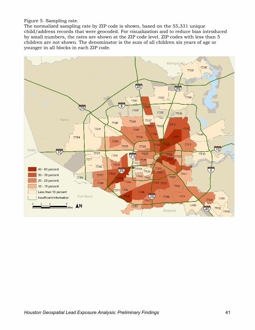
Houston Geospatial Lead Exposure Analysis: Preliminary Findings 41
Figure 5. Sampling rate. The normalized sampling rate by ZIP code is shown, based on the 55,331 unique child/address records that were geocoded. For visualization and to reduce bias introduced by small numbers, the rates are shown at the ZIP code level. ZIP codes with less than 5 children are not shown. The denominator is the sum of all children six years of age or younger in all blocks in each ZIP code.

Houston Geospatial Lead Exposure Analysis: Preliminary Findings 42
Figure 6. Blood-lead levels. Geographical distribution of study cohort (N = 55,329) by blood-lead levels 5 µg/dL or greater. BLL points are slightly shifted as described in Figure 2 and in the text to protect confidentiality.

Houston Geospatial Lead Exposure Analysis: Preliminary Findings 43
Figure 7. Year structure built. Maximum blood-lead level (BLL; N = 21,763) and residential parcels by year structure built (listed and estimated) for property code types A and B (N = 469,603 of a total of 597,710). Prior to 1950, residential paint was approximately 50% lead by weight. The child with the maximum BLL was chosen to represent a parcel in which more than one child resided. BLL points are repositioned to protect confidentiality as described in Figure 2 and in the text. For clarity, only BLLs ≥ 10 µg/dL are shown in this figure.

Houston Geospatial Lead Exposure Analysis: Preliminary Findings 44
Figure 8. Condition of housing. Maximum blood-lead level (BLL; N = 21,763) and residential parcels by condition of the housing unit for residential parcels state class code A and B (N = 406,087). The child with the maximum BLL was chosen to represent a parcel in which more than one child resided. BLL points are slightly shifted as described in Figure 2 and in the text to protect confidentiality. For clarity, only BLLs ≥ 10 µg/dL are shown in this figure.

Houston Geospatial Lead Exposure Analysis: Preliminary Findings 45
Figure 9. Median household income. Maximum blood-lead level (BLL; N = 21,763) and residential parcels type A and B (N = 406,087) by median household income (block group; N = 1,159). The child with the maximum BLL was chosen to represent a parcel in which more than one child resided. BLL points are slightly shifted as described in Figure 2 and in the text to protect confidentiality. For clarity, only BLLs ≥ 10 µg/dL are shown in this figure.

Houston Geospatial Lead Exposure Analysis: Preliminary Findings 46
Figure 10. Percent Hispanic/Latino. Maximum blood-lead level (BLL; N = 21,763) and residential parcels state class code A and B (N = 406,087) by percent Hispanic/Latino (block; N = 8,086 of 9,222). The child with the maximum BLL was chosen to represent a parcel in which more than one child resided. BLL points are slightly shifted as described in Figure 2 and in the text to protect confidentiality. For clarity, only BLLs ≥ 10 µg/dL are shown.

Houston Geospatial Lead Exposure Analysis: Preliminary Findings 47
Figure 11. Education. Maximum blood-lead level (BLL; N = 21,763) and residential parcels type A and B (N = 406,087) by percent of individuals 25 years or older with some college (block; N = 1,158 of 1,159). The child with the maximum BLL was chosen to represent a parcel in which more than one child resided. BLL points are slightly shifted as described in Figure 2 and in the text to protect confidentiality. For clarity, only BLLs ≥ 10 µg/dL are shown in this figure.

Houston Geospatial Lead Exposure Analysis: Preliminary Findings 48
Figure 12. Predicted blood-lead levels by parcel. Predicted blood-lead levels (BLLs) in children 2 to 3 years of age in all class A and B residential parcels in the study area for which there was complete information (N = 358,887 of 406,087 state class code A or B of total 597,710 parcels) calculated from the final multivariate linear mixed-effect model (LMM) at the parcel level (Table 8), with percent Black by block excluded (see text) Actual BLLs (offset as described in Figure 2 and in the text to protect confidentiality), by parcel, are also shown; for visual clarity only BLLs ≥ 10 µg/dL are shown on this figure.

Houston Geospatial Lead Exposure Analysis: Preliminary Findings 49
Figure 13. Autocorrelation. Analysis of residual clustering using the local Moran’s I statistic (LM), a “decomposition” of the global Moran’s I statistic. The LM is a measure of the degree to which model results are affected by missing spatial variables. The residuals from the final multivariate linear mixed-effects model (LMM) at the parcel level (N = 19,553; Table 8) were used. For this analysis, an effective search radius of approximately 6,065 feet was used around each parcel centroid. Groups of statistically significant clusters of high residual values (red dots) are indicative of areas for which the model most likely underpredicts, whereas groups of statistically significant low residual values (yellow dots) are indicative of areas for which missing the model most overpredicts. The global P-value is 0.01, suggesting that additional variables may need to be included in the model. Approximately 600 observations are poorly predicted by the model, and many of these outliers are geographically clustered. This may be useful in determining additional variables for inclusion in the model.
Houston Geospatial Lead Exposure Analysis: Preliminary Findings 50
APPENDICES

Houston Geospatial Lead Exposure Analysis: Preliminary Findings 51
Appendix 1: Abbreviations.
A+P: Actual plus predicted year residential structure built
ATSDR: Agency for Toxic Substances and Disease Registry
BLIMS: Blood Lead Information and Management System
BLL: Blood-lead level
CLPPP: Childhood Lead Poisoning Prevention Program
GIS: Geographic Information Systems
EPA: United States Environmental Protection Agency
HCAD: Harris County Appraisal District
HDHHS: Houston Department of Health and Human Services
IQ: Intelligence quotient
IRB: Institutional Review Board
LMM: Linear mixed-effects model
LM: Local Moran’s I statistic
µg/dL: Micrograms per deciliter
STAR*Map: Southeast Texas Addressing and Referencing Map
State class code (selected, from HCAD; building type based on parcel use) A1: Residential, single-family A2: Residential, mobile homes A3: Residential, auxiliary buildings A4: Residential, 1/2 duplex B1: Residential, multi-family B2: Residential, two-family B3: Residential, three-family B4: Residential, four- or more-family C1–C3: Vacant lots D2: Agricultural land E1: Farm and ranch land, improved F1–F2: Commercial and industrial J1–J6: Utilities (electric, telephone, rail, gas, etc.) M3: Personal property mobile home O1–O2: Inventory X0-X8: Exempt (charitable, governmental, religious, private school, etc.) X9: Low-moderate income housing Z0–Z5: Condos
STELLAR: Systematic Tracking of Elevated Lead Levels and Remediation

Houston Geospatial Lead Exposure Analysis: Preliminary Findings 52
Appendix 2: SAS Script. Statistical script (SAS 9.2) for the key data examinations and univariate and multivariate models.
/**********************************************************************************************/ /* */ /* PI: Dr. Winifred Hamilton */ /* Protocol: Houston Geospatial Lead Exposure Analysis */ /* Program: HGLEA_Analysis.sas */ /* Input Files: HGLEA.COH_pacel_rsk, HGLEA.BLM_chd_addr_lab_gis_final_sort */ /* (SAS permanent data files) */ /* External Macros: Unifreq.sas, Unimean.sas, Crossfreq.sas, MeanTest.sas */ /* Output Files: COH_unique_parcel_21763_with_19554_predicted.dbf */ /* COH_597710_with_predicted_bll.dbf */ /* */ /* Author: Xuemei Wang */ /* Date Completed: July 17, 2009 */ /* Description: Generate summary statistics for BLL data, HCAD data and Census data */ /* Fit general linear mixed model for log(Max BLL) in parcel level data */ /* Compute the predicted blood lead level by parcel in COH */ /* */ /* SAS Version: 9.2 */ /**********************************************************************************************/ libname HGLEA 'P:\HGLEA Project\STATISTICS\COMBINED_STAT_DB_129855'; libname HGLEA2 'X:/HGLEA Project/Statistics/SAS Data'; %include "X:\HGLEA Project\STATISTICS\SAS codes\SAS Macro\UniFreq.sas"; %include "X:\HGLEA Project\STATISTICS\SAS codes\SAS Macro\UniMean.sas"; %include "X:\HGLEA Project\STATISTICS\SAS codes\SAS Macro\CrossFreq.sas"; %include "X:\HGLEA Project\STATISTICS\SAS codes\SAS Macro\MeansTest.sas"; run; /*************** Import COH parcels with all risk factors from HCAD and Census data base ***********/ PROC IMPORT OUT= HGLEA.COH_pacel_rsk DATAFILE= "X:\HGLEA Project\Final Data\rsk_red.dbf" DBMS=DBF REPLACE; GETDELETED=NO; RUN; /*** unique by HCAD Number ***/ proc contents data= HGLEA.COH_pacel_rsk varnum; /** N = 597710 **/ run; /*************** Import BLIMS data: address table ************/ PROC IMPORT OUT= HGLEA.BLIMS_address DATATABLE= 'AddressUnder62004-2008' DBMS=ACCESS REPLACE; DATABASE='X:\HGLEA Project\STATISTICS\COMBINED_STAT_DB_129855\BLIMS_20090626.mdb'; SCANMEMO=YES; USEDATE=yes; SCANTIME=YES; RUN ;proc contents data=HGLEA.BLIMS_address; /*** n = 141496 ***/ run; proc sort data =HGLEA.BLIMS_address out = test_addrID nodupkey; by addr_ID; run; /*************** Import BLIMS data: child table ************/ PROC IMPORT OUT= HGLEA.BLIMS_child DATATABLE= 'ChildUnder62004-2008' DBMS=ACCESS REPLACE; DATABASE='X:\HGLEA Project\STATISTICS\COMBINED_STAT_DB_129855\BLIMS_20090626.mdb'; SCANMEMO=YES; USEDATE=yes; SCANTIME=YES; RUN; proc contents data=HGLEA.BLIMS_child; /*** n = 141496 ***/ run; /*************** Import BLIMS data: lab table ************/ PROC IMPORT OUT= HGLEA.BLIMS_lab DATATABLE= 'LabUnder62004-2008' DBMS=ACCESS REPLACE; DATABASE='X:\HGLEA Project\STATISTICS\COMBINED_STAT_DB_129855\BLIMS_20090626.mdb';
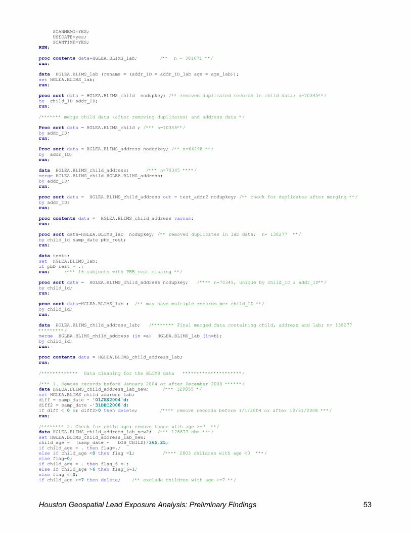
Houston Geospatial Lead Exposure Analysis: Preliminary Findings 53
SCANMEMO=YES; USEDATE=yes; SCANTIME=YES; RUN; proc contents data=HGLEA.BLIMS_lab; /** n = 381671 **/ run; data HGLEA.BLIMS_lab (rename = (addr_ID = addr_ID_lab age = age_lab)); set HGLEA.BLIMS_lab; run; proc sort data = HGLEA.BLIMS_child nodupkey; /** removed duplicated records in child data; n=70345**/ by child_ID addr_ID; run; /******* merge child data (after removing duplicates) and address data */ Proc sort data = HGLEA.BLIMS_child ; /*** n=70345**/ by addr_ID; run; Proc sort data = HGLEA.BLIMS_address nodupkey; /** n=64298 **/ by addr_ID; run; data HGLEA.BLIMS_child_address; /*** n=70345 ****/ merge HGLEA.BLIMS_child HGLEA.BLIMS_address; by addr_ID; run; proc sort data = HGLEA.BLIMS_child_address out = test_addr2 nodupkey; /** check for duplicates after merging **/ by addr_ID; run; proc contents data = HGLEA.BLIMS_child_address varnum; run; proc sort data=HGLEA.BLIMS_lab nodupkey; /** removed duplicates in lab data; n= 138277 **/ by child_id samp_date pbb_rest; run; data testt; set HGLEA.BLIMS_lab; if pbb_rest = .; run; /*** 16 subjects with PBB_rest missing **/ proc sort data = HGLEA.BLIMS_child_address nodupkey; /**** n=70345, unique by child_ID & addr_ID**/ by child_id; run; proc sort data=HGLEA.BLIMS_lab ; /** may have multiple records per child_ID **/ by child_id; run; data HGLEA.BLIMS_child_address_lab; /******** Final merged data containing child, address and lab; n= 138277 *********/ merge HGLEA.BLIMS_child_address (in =a) HGLEA.BLIMS_lab (in=b); by child_id; run; proc contents data = HGLEA.BLIMS_child_address_lab; run; /************* Data cleaning for the BLIMS data *********************/ /*** 1. Remove records before January 2004 or after December 2008 ******/ data HGLEA.BLIMS_child_address_lab_new; /*** 129855 */ set HGLEA.BLIMS_child_address_lab; diff = samp_date - '01JAN2004'd; diff2 = samp_date -'31DEC2008'd; if diff < 0 or diff2>0 then delete; /**** remove records before 1/1/2004 or after 12/31/2008 ***/ run; /******** 2. Check for child_age; remove those with age >=7 **/ data HGLEA.BLIMS_child_address_lab_new2; /*** 128677 obs ***/ set HGLEA.BLIMS_child_address_lab_new; child_age = (samp_date - DOB_CHILD)/365.25; if child_age = . then flag=.; else if child_age <0 then flag =1; /**** 2803 children with age <0 ***/ else flag=0; if child_age = . then flag_6 =.; else if child_age >6 then flag_6=1; else flag_6=0; if child_age >=7 then delete; /** exclude children with age >=7 **/

Houston Geospatial Lead Exposure Analysis: Preliminary Findings 54
run; proc freq data = HGLEA.BLIMS_child_address_lab_new2; tables flag; run; /*** ******* * GIS Map data ********/ PROC IMPORT OUT= HGLEA.GIS_MAP DATAFILE= "X:\HGLEA Project\GIS_MAPS\gis_layers_3\unique_list_w_codes.dbf" DBMS=DBF REPLACE; GETDELETED=NO; RUN; proc contents data = HGLEA.gis_map; /** n= 38201 **/ run; proc sort data=HGLEA.gis_map (rename = (ADDR_ID = ADDR_ID_GIS)); /** records have unique ASSEMADDR **/ by ASSEMADDR; run; proc sort data= HGLEA.BLIMS_child_address_lab_new2 ; by ASSEMADDR; run; data HGLEA.BLIMS_child_address_lab_gis; /*** 128677 ***/ merge HGLEA.BLIMS_child_address_lab_new2(in=a) HGLEA.gis_map (in=b); by ASSEMADDR; if a; /** keep only those records with corresponding addr_id in the child_address_lab_new2 data*/ run; proc contents data= HGLEA.BLIMS_child_address_lab_gis varnum; run; data HGLEA.BLIMS_child_address_lab_gis_c; /** n= 119221 **/ set HGLEA.BLIMS_child_address_lab_gis; if geo_type = 5 or geo_type =2 then delete; /** remove 5 = in Houston, but outside Harris; 2 = outside of houston **/ run; proc contents data= HGLEA.BLIMS_child_address_lab_gis_c; run; /*** compare geo_type = 3 or 4 (matched) vs. geo_type =1 (fail to match) in regard to characteristics **/ proc contents data= HGLEA.BLIMS_child_address_lab_gis_c; run; proc sort data=HGLEA.BLIMS_child_address_lab_gis_c; /*** n=119221 **/ by addr_id child_id pbb_rest; run; /*** keep max blood lead level for each child **/ data HGLEA.BLIMS_child_address_lab_gis_c2 (rename = (pbb_rest = max_pbb_rest)); /** n=64460 **/ set HGLEA.BLIMS_child_address_lab_gis_c; by addr_id child_id pbb_rest; if last.child_id; /* keep the last records, which is the largest blood lead level **/ run; proc univariate data = HGLEA.BLIMS_child_address_lab_gis_c2 ; var max_pbb_rest; run; /*** calculate mean blood lead level for each child ; n= 119221 **/ proc sql; create table HGLEA.BLIMS_child_address_lab_gis_c3 as select *, mean(pbb_rest) as mean_pbb_rest from HGLEA.BLIMS_child_address_lab_gis_c group by addr_id, child_id; quit; proc contents data = HGLEA.BLIMS_child_address_lab_gis_c3; run; data HGLEA.BLIMS_child_address_lab_gis_c3; /*** n=64460 **/ set HGLEA.BLIMS_child_address_lab_gis_c3; keep addr_id child_id pbb_rest mean_pbb_rest; proc sort data =HGLEA.BLIMS_child_address_lab_gis_c3 ; by addr_id child_id pbb_rest; run; data HGLEA.BLIMS_child_address_lab_gis_c3 (drop = pbb_rest); /** n=64460; it does not matter which record to keep; they all have the mean lab value **/ set HGLEA.BLIMS_child_address_lab_gis_c3; by addr_id child_id pbb_rest; if last.child_id; run;
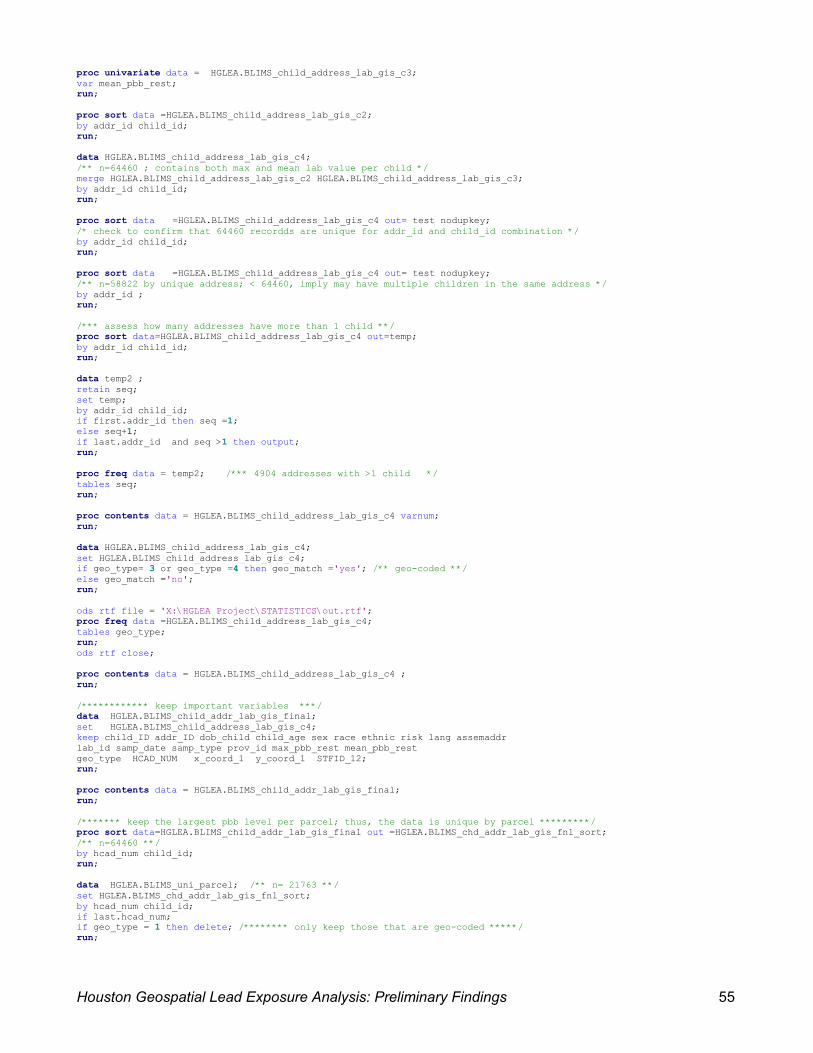
Houston Geospatial Lead Exposure Analysis: Preliminary Findings 55
proc univariate data = HGLEA.BLIMS_child_address_lab_gis_c3; var mean_pbb_rest; run; proc sort data =HGLEA.BLIMS_child_address_lab_gis_c2; by addr_id child_id; run; data HGLEA.BLIMS_child_address_lab_gis_c4; /** n=64460 ; contains both max and mean lab value per child */ merge HGLEA.BLIMS_child_address_lab_gis_c2 HGLEA.BLIMS_child_address_lab_gis_c3; by addr_id child_id; run; proc sort data =HGLEA.BLIMS_child_address_lab_gis_c4 out= test nodupkey; /* check to confirm that 64460 recordds are unique for addr_id and child_id combination */ by addr_id child_id; run; proc sort data =HGLEA.BLIMS_child_address_lab_gis_c4 out= test nodupkey; /** n=58822 by unique address; < 64460, imply may have multiple children in the same address */ by addr_id ; run; /*** asse ss how many addresses have more than 1 child **/ proc sort data=HGLEA.BLIMS_child_address_lab_gis_c4 out=temp; by addr_id child_id; run; data temp2 ; retain seq; set temp; by addr_id child_id; if first.addr_id then seq =1; else seq+1; if last.addr_id and seq >1 then output; run; proc freq data = temp2; /*** 4904 addresses with >1 child */ tables seq; run; proc contents data = HGLEA.BLIMS_child_address_lab_gis_c4 varnum; run; data HGLEA.BLIMS_child_address_lab_gis_c4; set HGLEA.BLIMS_child_address_lab_gis_c4; if geo_type= 3 or geo_type =4 then geo_match ='yes'; /** geo-coded **/ else geo_match ='no'; run; ods tf fr ile = 'X:\HGLEA Project\STATISTICS\out.rtf'; proc freq data =HGLEA.BLIMS_child_address_lab_gis_c4; tables geo_type; run; ods rtf close; proc contents data = HGLEA.BLIMS_child_address_lab_gis_c4 ; run; /************ keep important variables ***/ data HGLEA.BLIMS_child_addr_lab_gis_final; set HGLEA.BLIMS_child_address_lab_gis_c4; keep child_ID addr_ID dob_child child_age sex race ethnic risk lang assemaddr lab_id samp_date samp_type prov_id max_pbb_rest mean_pbb_rest geo_type HCAD_NUM x_coord_1 y_coord_1 STFID_12; run; proc contents data = HGLEA.BLIMS_child_addr_lab_gis_final; run; /******* keep the largest pbb level per parcel; thus, the data is unique by parcel *********/ proc sort data=HGLEA.BLIMS_child_addr_lab_gis_final out =HGLEA.BLIMS_chd_addr_lab_gis_fnl_sort; /** n=64460 **/ by hcad_num child_id; run; data HGLEA.BLIMS_uni_parcel; /** n= 21763 **/ set HGLEA.BLIMS_chd_addr_lab_gis_fnl_sort; by hcad_num child_id; if last.hcad_num; if geo_type = 1 then delete; /******** only keep those that are geo-coded *****/ run;
Houston Geospatial Lead Exposure Analysis: Preliminary Findings 56
/*** ***** * Export data into dbasse format ************/ PROC EXPORT DATA= HGLEA.BLIMS_uni_parcel OUTFILE= "X:\HGLEA Project\Final Data\BLIMS_GIS_unique_parcel_21763.dbf" DBMS=DBF REPLACE; RUN; /** summary statistics for categorical and continuous variabels **/ ods rtf file = 'X:\HGLEA Project\STATISTICS\out.rtf'; %unifreq (data=HGLEA.BLIMS_child_address_lab_gis_c4, variable =sex race ethnic risk samp_type addr_zip, nvar=6); run; %unimean (data=HGLEA.BLIMS_child_address_lab_gis_c4, variable =child_age max_pbb_rest mean_pbb_rest , nvar=3); run; ods rtf close; ods rtf file = 'X:\HGLEA Project\STATISTICS\out.rtf'; %CrossFreq(data=HGLEA.BLIMS_child_address_lab_gis_c4,variable=sex race ethnic risk, nvar=4, byvar=geo_match, nlev=2, lev=no yes); run; ods rtf close; ods rtf file = 'X:\HGLEA Project\STATISTICS\out.rtf'; %meanstest(data=HGLEA.BLIMS_child_address_lab_gis_c4,variable=child_age max_pbb_rest mean_pbb_rest ,nvar=3,byvar=geo_match, nlev=2); run; ods rtf close; /*************************************************************/ /************** Merge COH parcel data and BLIMS data *********/ /*************************************************************/ proc sort data =HGLEA.COH_pacel_rsk out =HGLEA.COH_pacel_rsk_sorted; /** N = 597710 **/ by hcad_num; run; /*** ***** * N= 64460; including geo-coded (geo_type = 3,4) and not geo-coded (geo_type =1) ***/ proc sort data=HGLEA.BLIMS_child_addr_lab_gis_final out=HGLEA.BLM_chd_addr_lab_gis_final_sort (drop =x_coord_1 y_coord_1 STFID_12);/* N = 64460*/ by hcad_num; run; data HGLEA.BLIMS_COH_Parcel_64460; /*** N = 64460 ***/ merge HGLEA.COH_pacel_rsk_sorted (in =a) HGLEA.BLM_chd_addr_lab_gis_final_sort (in=b); by hcad_num; if b; run; /** N= 55331; geo-coded only (geo_type = 3,4) **/ data HGLEA.BLM_chd_addr_lab_gis_final_sort2; set HGLEA.BLM_chd_addr_lab_gis_final_sort; if hcad_num ^= ''; run; data HGLEA.BLIMS_COH_Parcel_55331; /*** N= 55331 ***/ merge HGLEA.COH_pacel_rsk_sorted (in =a) HGLEA.BLM_chd_addr_lab_gis_final_sort2 (in=b); by hcad_num; if b; run; proc contents data=HGLEA.BLIMS_COH_Parcel_55331 varnum;/*** 55331, geo_type = 3 or 4, unique by HCAD number */ run; proc contents data=HGLEA.BLIMS_COH_Parcel_64460 varnum;/* 64460,geo_type = 1, 3 or 4, unique by HCAD number */ run; /********* Summary Statistics N=64460 merged data set *********/ data HGLEA.BLIMS_COH_Parcel_64460; /*** 64460, geo_type = 1, 3 or 4, unique by HCAD number */ length state_clas_new $20 yr_built_group $20 imp_val_per_sf_group $ 20 quality_group $20 age_group $20; set HGLEA.BLIMS_COH_Parcel_64460; /***** Age *******/ if child_age = . then age_group=''; else if child_age >= 0 & child_age<1 then age_group='1: 0 to < 1 yr'; else if child_age >= 1 & child_age<2 then age_group='2: 1 to < 2 yr'; else if child_age >= 2 & child_age<3 then age_group='3: 2 to < 3 yr'; else if child_age >= 3 & child_age<4 then age_group='4: 3 to < 4 yr'; else if child_age >= 4 & child_age<5 then age_group='5: 4 to < 5 yr'; else if child_age >= 5 & child_age<6 then age_group='6: 5 to < 6 yr'; else if child_age >= 6 & child_age<7 then age_group='7: 6 to < 7 yr'; /***** Sex *******/ if sex = '' then sex_group =''; else if sex ='F' then sex_group='Female'; else if sex ='M' then sex_group ='Male'; else sex_group ='Other';

Houston Geospatial Lead Exposure Analysis: Preliminary Findings 57
/***** Race and Ethnicity *******/ if ethnic ='H' then race_ethnic ='2: Hispanic/Latino'; else if ethnic ^='H' and race = '5' then race_ethnic = '1: White'; else if ethnic ^='H' and race ='3' then race_ethnic = '3: Black'; else if ethnic ^='H' and race ='2' then race_ethnic = '4: Asian'; else if ethnic ^='H' and race ='1' or race ='4' or race ='7' or race ='8' or race='9' then race_ethnic ='5: Other'; else race_ethnic =''; /***** Building Style *******/ if state_clas = '' then state_clas_new =''; else if state_clas = 'A1' then state_clas_new = '1: A1'; else if state_clas ='A2' | state_clas = 'A3' | state_clas = 'A4' then state_clas_new ='2: A2, A3 or A4'; else if state_clas ='B1' then state_clas_new ='3: B1'; else if state_clas ='B2' | state_clas = 'B3' | state_clas = 'B4' then state_clas_new = '4: B2, B3 or B4'; else if state_clas ='X1' | state_clas ='X2' | state_clas ='X3' |state_clas ='X4' | state_clas ='X5' | state_clas ='X9' then state_clas_new = '5: X1 -X9'; else if state_clas ='Z1' | state_clas ='Z2' | state_clas ='Z3' |state_clas ='Z4' | state_clas ='Z5' then state_clas_new = '6: Z1 - Z5'; else state_clas_new = '7: Other'; /***** Year built *******/ yr_res_built = input(DATE_ERECT, best8.); if yr_res_built = . the _built_group = ''; n yrelse if yr_res_built <=1950 then yr_built_grou '1: <= 1950'; p = else if yr_res_built > 1950 & yr_res_built <= 1978 then yr_built_group = '2: >1950 to <= 1978'; else if yr_res_built >1978 then yr_built_group = '3: > 1978'; /******* quality *********/ if quality = '' then quality_group =''; else if quality ='A' then quality_group ='6: Excellent'; else if quality ='B' then quality_group ='5: Good'; else if quality ='C' then quality_group ='4: Above average'; else if quality ='D' then quality_group ='3: Average'; else if quality ='E' then quality_group ='2: Fair'; else if quality ='F' then quality_group ='1: Poor'; /****** improvement value per sq ft for living area ******/ heat_area_n = input(heat_area, best8.); if heat_area_n = . or heat_area_n =0 then imp_val_per_Sf =.; else imp_val_per_Sf = improvemen/heat_area_n; if imp_val_per_Sf = . then imp_val_per_sf_group = ''; else if imp_val_per_Sf <=25 then imp_val_per_sf_group = '1: <= 25 '; else if imp_val_per_Sf >25 and imp_val_per_Sf <=50 then imp_val_per_sf_group = '2: >25 to <=50'; else if imp_val_per_Sf >50 and imp_val_per_Sf <=100 then imp_val_per_sf_group = '3: >50 to <=100'; else if imp_val_per_Sf >100 then imp_val_per_sf_group = '4: >100'; run; /******* BLL summary ******/ /****** 1. N=119221, all available data from COH with geo_type = 1, 3 or 4 ******/ proc univariate data= HGLEA.BLIMS_child_address_lab_gis_c; var pbb_rest; run; /****** 2. N= 64460, all subjects with geo_type = 1, 3 or 4 and kept only the max BLL for each subject **/ proc univariate data= HGLEA.BLIMS_child_address_lab_gis_c4; var max_pbb_rest; run; /****** 3. N= 58822, based on 2 above, extracted max BLL per address ID ***/ proc sort data=HGLEA.BLIMS_child_address_lab_gis_c4 out=tempp; by addr_id max_pbb_rest; run; data tempp2 (rename=(max_pbb_rest = max_pbb_rest_per_addr)); set tempp; by addr_id max_pbb_rest ; if last.addr_id; /* keep the last records, which is the largest blood lead level for a given addr_ID **/ run; proc univariate data = tempp2; var max_pbb_rest_per_addr; run; /*** ********* **** Summary of BLL by age, gender, race and other HCAD category **********/ proc contents data=HGLEA.BLIMS_COH_Parcel_64460 varnum;/* 64460, geo_type = 1, 3 or 4, unique by HCAD number */ run; proc sort data = HGLEA.BLIMS_COH_Parcel_64460 out=temp ; by sex; run;

Houston Geospatial Lead Exposure Analysis: Preliminary Findings 58
proc univariate data= temp; var max_pbb_rest; by sex; run; proc sort data = HGLEA.BLIMS_COH_Parcel_64460 out=temp ; by race_ethnic; run ;proc univariate data= temp; var max_pbb_rest; by race_ethnic; run; proc sort data = HGLEA.BLIMS_COH_Parcel_64460 out=temp ; by age_group; run; proc univariate data= temp; var max_pbb_rest; by age_group; run; proc sort data = HGLEA.BLIMS_COH_Parcel_64460 out=temp ; by state_clas_new; run ;proc univariate data= temp; var max_pbb_rest; by state_clas_new; run; proc sort data = HGLEA.BLIMS_COH_Parcel_64460 out=temp ; by yr_built_group; run; proc univariate data= temp; var max_pbb_rest; by yr_built_group; run; proc sort data = HGLEA.BLIMS_COH_Parcel_64460 out=temp ; by quality_group; run ;proc univariate data= temp; var max_pbb_rest; by quality_group; run; proc sort data = HGLEA.BLIMS_COH_Parcel_64460 out=temp ; by imp_val_per_sf_group ; run; proc univariate data= temp; var max_pbb_rest; by imp_val_per_sf_group ; run; /*********************************************************************/ /* */ /* from here on, all analyses will be based on N = 55331 obs */ /* */ /*******************************************************************/ /**** summary of BLL based on 55331 geo_coded records,i.e., with geo_type = 3 or 4 ******/ proc contents data=HGLEA.BLIMS_COH_Parcel_55331 varnum; /*** N = 55331, geo_type = 3 or 4 */ run; data HGLEA.BLIMS_COH_Parcel_55331; /*** N = 55331, geo_type = 3 or 4 */ length state_clas_new $20 yr_built_group $20 imp_val_per_sf_group $ 20 quality_group $20 sex_group $6 age_group $20 race_ethnic $20; set HGLEA.BLIMS_COH_Parcel_55331; /***** Age *******/ if child_age = . then age_group=''; else if child_age >= 0 & child_age<1 then age_group='1: 0 to < 1 yr'; else if child_age >= 1 & child_age<2 then age_group='2: 1 to < 2 yr'; else if child_age >= 2 & child_age<3 then age_group='3: 2 to < 3 yr'; else if child_age >= 3 & child_age<4 then age_group='4: 3 to < 4 yr'; else if child_age >= 4 & child_age<5 then age_group='5: 4 to < 5 yr'; else if child_age >= 5 & child_age<6 then age_group='6: 5 to < 6 yr'; else if child_age >= 6 & child_age<7 then age_group='7: 6 to < 7 yr'; if child_age = . then ''; age_group_new=else if child_age >= 0 & child_age<2 then age_group_new='1: 0 to < 2 yr'; else if child_age >= 2 & child_age<3 then age_group_new='2: 2 to < 3 yr'; else if child_age >= 3 & child_age<5 then age_group_new='3: 3 to < 5 yr'; else if child_age >= 5 & child_age<7 then age_group_new='4: 5 to < 7 yr';

Houston Geospatial Lead Exposure Analysis: Preliminary Findings 59
/***** Sex *******/ if sex = '' then sex_group =''; else if sex ='F' then sex_group='Female'; else if sex ='M' then sex_group ='Male'; else sex_group ='Other'; /***** Race and Ethnicity *******/ if ethnic ='H' then race_ethnic ='2: Hispanic/Latino'; else if ethnic ^='H' and race = '5' then race_ethnic = '1: White'; else if ethnic ^='H' and race ='3' then race_ethnic = '3: Black'; else if ethnic ^='H' and race ='2' then race_ethnic = '4: Asian'; else if ethnic ^='H' and race ='1' or race ='4' or race ='7' or race ='8' or race='9' then race_ethnic ='5: Other'; else race_ethnic =''; /***** Building Style *******/ if state_clas = '' then state_clas_new =''; else if state_clas = 'A1' then state_clas_new = '1: A1'; else if state_clas ='A2' | state_clas = 'A3' | state_clas = 'A4' then state_clas_new ='2: A2, A3 or A4'; else if state_clas ='B1' then state_clas_new ='3: B1'; else if state_clas ='B2' | state_clas = 'B3' | state_clas = 'B4' then state_clas_new = '4: B2, B3 or B4'; else if state_clas ='X1' | state_clas ='X2' | state_clas ='X3' |state_clas ='X4' | state_clas ='X5' | state_clas ='X9' then state_clas_new = '5: X1 -X9'; else if state_clas ='Z1' | state_clas ='Z2' | state_clas ='Z3' |state_clas ='Z4' | state_clas ='Z5' then state_clas_new = '6: Z1 - Z5'; else state_clas_new = '7: Other'; if state_clas_new = '' then state_class_final =''; else if state_clas_new ='1: A1' or state_clas_new = '2: A2, A3 or A4' then state_class_final = 'A'; else if state_clas_new ='3: B1' or state_clas_new = '4: B2, B3 or B4' then state_class_final ='B'; else if state_clas_new = '5: X1 -X9' or state_clas_new = '6: Z1 - Z5' or state_clas_new = '7: Other' then state_class_final='Other'; /***** year bulit *******/ yr_res_built = input(DATE_ERECT, best8.); if yr_res_built = . the _built_group = ''; n yrelse if yr_res_built <=1950 then yr_built_grou '1: <= 1950'; p = else if yr_res_built > 1950 & yr_res_built <= 1978 then yr_built_group = '2: >1950 to <= 1978'; else if yr_res_built >1978 then yr_built_group = '3: > 1978'; /******* quality *********/ if quality = '' then quality_group =''; else if quality ='A' then quality_group ='6: Excellent'; else if quality ='B' then quality_group ='5: Good'; else if quality ='C' then quality_group ='4: Above average'; else if quality ='D' then quality_group ='3: Average'; else if quality ='E' then quality_group ='2: Fair'; else if quality ='F' then quality_group ='1: Poor'; /****** improvement value per sq ft living area ******/ heat_area_n = input(heat_area, best8.); if heat_area_n = . or heat_area_n =0 then imp_val_per_Sf =.; else imp_val_per_Sf = improvemen/heat_area_n; if imp_val_per_Sf = . then imp_val_per_sf_group = ''; else if imp_val_per_Sf <30 then imp_val_per_sf_group = '1: <30 '; else if imp_val_per_Sf >=30 and imp_val_per_Sf < 45 then imp_val_per_sf_group = '2: >=30 to < 45'; else if imp_val_per_Sf >=45 and imp_val_per_Sf < 55 then imp_val_per_sf_group = '3: >=45 to < 55'; else if imp_val_per_Sf >=55 then imp_val_per_sf_group = '4: >=55'; run; proc univariate data= HGLEA.BLIMS_COH_Parcel_55331; var max_pbb_rest; run; proc sort data = HGLEA.BLIMS_COH_Parcel_55331 out=temp ; by age_group; run ;proc univariate data= temp; var max_pbb_rest; by age_group; run; proc sort data = HGLEA.BLIMS_COH_Parcel_55331 out=temp ; by sex_group; run; proc univariate data= temp; var max_pbb_rest; by sex_group; run; proc sort data = HGLEA.BLIMS_COH_Parcel_55331 out=temp ; by race_ethnic; run; proc univariate data= temp;

Houston Geospatial Lead Exposure Analysis: Preliminary Findings 60
var max_pbb_rest; by race_ethnic; run; proc sort data = HGLEA.BLIMS_COH_Parcel_55331 out=temp ; by yr_built_group; run ;proc univariate data= temp; var max_pbb_rest; by yr_built_group; run; proc sort data = HGLEA.BLIMS_COH_Parcel_55331 out=temp ; by imp_val_per_sf_group ; run; proc univariate data= temp; var max_pbb_rest; by imp_val_per_sf_group ; run; proc sort data = HGLEA.BLIMS_COH_Parcel_55331 out=temp ; by state_clas_new; run ;proc univariate data= temp; var max_pbb_rest; by state_clas_new; run; proc sort data =HGLEA.BLIMS_COH_Parcel_55331 out=temp ; by quality_group; run; proc univariate data= temp; var max_pbb_rest; by quality_group; run; /*************** Census block level data summary *************/ data HGLEA.BLIMS_COH_Parcel_55331; set HGLEA.BLIMS_COH_Parcel_55331; N_white = input(P008003, best8.); N_black = input(P008004, best8.); N_asian = input(P008006, best8.); N_hispanic = sum( input(P008011, best8.), input(P008012, best8.), input(P008013, best8.), input(P008014, best8.), input(P008015, best8.), input(P008016, best8.)); N_others= sum(input(P008005, best8.), input(P008007, best8.), input(P008008, best8.)); N_total = sum(N_white,N_black, N_asian, N_hispanic, N_others); percent_white = N_white *100 /N_total; percent_black = N_black *100 /N_total; percent_asian = N_asian *100 /N_total; percent_hispanic = N_hispanic *100 /N_total; percent_others = N_others *100 /N_total; percent_owner = input(H004002, best8.) *100 input(H004001, best8.); /percent_renter = input(H004003, best8.) *100/ input(H004001, best8.); run; proc contents data = HGLEA.BLIMS_COH_Parcel_55331; run; /******* calculate Living density (sq ft heated / person) *****/ /***** total populaiton in each block : p003001 *******/ /****** n= 597710 *****/ proc sql; create table heat_area_per_block as select stfid_12, heat_area, sum(input(heat_area, best8.)) as total_heat_area_per_block from HGLEA.COH_pacel_rsk group by stfid_12; quit; proc univariate data = heat_area_per_block ; var total_heat_area_per_block; run; proc sort data =heat_area_per_block out = heat_area_per_block_sorted (drop=heat_area) nodupkey; /** n=20692; get the total heat area per unique block **/ by stfid_12; run; proc sort data = HGLEA.BLIMS_COH_Parcel_55331 out=HGLEA.BLIMS_COH_Parcel_55331; by stfid_12 ; run; data HGLEA.BLIMS_COH_Parcel_55331_new; merge heat_area_per_block_sorted (in=a) HGLEA.BLIMS_COH_Parcel_55331(in=b); by stfid_12;

Houston Geospatial Lead Exposure Analysis: Preliminary Findings 61
if b; run; data HGLEA.BLIMS_COH_Parcel_55331_new; set HGLEA.BLIMS_COH_Parcel_55331_new; if p003001 = 0 then living_density = .; else living_density = total_heat_area_per_block/p003001; /** p003001 = total population per block **/ run; proc sort data = HGLEA.BLIMS_COH_Parcel_55331_new out=temp nodupkey; /** take unique blocks; n_unique_block = 9222 **/ by stfid_12 ; run; proc univariate data=temp; var p003001 percent_white percent_black percent_asian percent_hispanic percent_others percent_owner percent_renter living_density; label p003001 ='Total population'; run; /******* Summary of Census Block Group data ********/ data HGLEA.BLIMS_COH_Parcel_55331_new2 ; set HGLEA.BLIMS_COH_Parcel_55331_new ; /***** year structure built (Block Group) *******/ N_before_50 = H034010 + H034009; N_50_to_79 = H034008 + H034007 + H034006; N_after_79 = H034005 + H034004 + H034003 + H034002; N_total_yr = N_before_50 + N_50_to_79+ N_after_79; if N_total_yr = 0 then do; percent_before_50 = .; percent_50_to_79 =.; percent_after_79= .; end; else do; percent_before_50 = N_before_50 100/ N_total_yr ; *percent_50_to_79 = N_50_to_79*100 / N_total_yr ; percent_after_79 = N_after_79*100 / N_total_yr ; end; /*** Education: some college - doctorate degree in >=25 yrs old**/ /*male */ N_male_some_college = sum(P037012, P037013, P037014, P037015, P037016, P037017 ,P037018); /*female */ N_female_some_college = sum(P037029, P037030, P037031,P037032, P037033, P037034, P037035); N_some_college = sum(N_male_some_college, N_female_some_college); if P037001 = 0 then percent_some_college = .; else percent_some_college = N_some_college *100 / P037001; /** P037001 = toal population per block group **/ stfid_bg_m =substr(stfid_12, 1, 12); run; proc sort data = HGLEA.BLIMS_COH_Parcel_55331_new2 out=temp_block_group nodupkey; /** n= 1159 unique block group **/ by stfid_bg_m ; run; proc univariate data= temp_block_group; var percent_before_50 percent_50_to_79 percent_after_79 percent_some_college P053001; label P053001 ='Median household income in 1999'; run; /*********** Prepare variables before fitting LMM **********/ data HGLEA.BLIMS_COH_Parcel_55331_new3; set HGLEA.BLIMS_COH_Parcel_55331_new2; length state_class_final $5 quality_group_final $20; stfid_bg_m =substr(stfid_12, 1, 12 ; )if max_pbb_rest =. then pbb_0_yes=.; else if max_pbb_rest = 0 then pbb_0_yes = 1; else pbb_0_yes =0; if max_pbb_rest = . then max_pbb_new =.; else if max_pbb_rest = 0 then max_pbb_new =0.1; else max_pbb_new = max_pbb_rest; lg_max_pbb = log(max_pbb_new); if sex ='U' or sex ='Z' the male =.; nelse if sex 'M' then male =1; =else male =0; if state_clas_new = '' then state_class_final =''; else if state_clas_new ='1: A1' or state_clas_new = '2: A2, A3 or A4' then state_class_final = 'A'; else if state_clas_new ='3: B1' or state_clas_new = '4: B2, B3 or B4' then state_class_final ='B';

Houston Geospatial Lead Exposure Analysis: Preliminary Findings 62
else if state_clas_new = '5: X1 -X9' or state_clas_new = '6: Z1 - Z5' or state_clas_new = '7: Other' then state_class_final='Other'; quality_group_final = quality_group; if quality_group ='5: Good' or quality_group = '6: Excellent' then quality_group_final ='5: Good/Excellent'; Median_income = P053001/1000; /** median household income (x $1000)*/ total_pop = P003001/100; living_density_new = living_density/100; run; proc freq data=HGLEA.BLIMS_COH_Parcel_55331_new3 ; /** we have 1015 subjects with max_pbb_rest = 0 -> set to 0.1 for analysis */ tables pbb_0_yes sex*male state_clas_new * state_class_final quality_group * quality_group_final; run; /******** replace missing data on yr_built (parcel level data) with predicted values **/ data HGLEA.BLIMS_COH_Parcel_55331_new3; set HGLEA.BLIMS_COH_Parcel_55331_new3; improve_value = improvemen/100000; run; proc univariate data= HGLEA.BLIMS_COH_Parcel_55331_new3; var improve_value percent_before_50 percent_50_to_79 percent_after_79 percent_black; run; proc freq data = HGLEA.BLIMS_COH_Parcel_55331_new3; tables state_class_final; run; proc mixed data = HGLEA.BLIMS_COH_Parcel_55331_new3 nclprint; class stfid_bg_m state_class_final; model yr_res_built = state_class_final improve_value percent_before_50 percent_50_to_79 percent_after_79/solution cl outp=predicted_yr_built; random int/type=un subject =stfid_bg_m; run; proc univariate data = predicted_yr_built; var pred; run; proc sort data = predicted_yr_built (keep = hcad_num yr_res_built pred rename=(yr_res_built =yr_res_built_old pred=pred_yr_built)) out = predicted_yr_built_sorted nodupkey; by hcad_num; run; proc sort data=HGLEA.BLIMS_COH_Parcel_55331_new3; by hcad_num; run; data HGLEA.BLIMS_COH_Parcel_55331_new3; merge HGLEA.BLIMS_COH_Parcel_55331_new3 predicted_yr_built_sorted; by hcad_num; run; /******* the variable yar_res_built has both actual and predicted values ********/ data HGLEA.BLIMS_COH_Parcel_55331_new3; set HGLEA.BLIMS_COH_Parcel_55331_new3; yr_res_built_new= yr_res_built; if yr_res_built = . then yr_res_built_new =pred_yr_built; if yr_res_built_new = . the _built_group = ''; n yrelse if yr_res_built_new <=1950 then yr_built_grou '1: <= 1950'; p = else if yr_res_built_new > 1950 & yr_res_built <= 1978 then yr_built_group = '2: >1950 to <= 1978'; else if yr_res_built_new >1978 then yr_built_group = '3: > 1978'; run; proc univariate data = HGLEA.BLIMS_COH_Parcel_55331_new3; var pred_yr_built; run; proc sort data = HGLEA.BLIMS_COH_Parcel_55331_new3 out = HGLEA.BLIMS_COH_55331_sorted; by hcad_num max_pbb_rest; run; data HGLEA.BLIMS_COH_55331_unique_parcel; /***** N = 21763 unique parcels *****/ set HGLEA.BLIMS_COH_55331_sorted; by hcad_num max_pbb_rest; if last.hcad_num; /**** take the largest BLL level in a parcel, if a parcel has more than 1 child ****/ run; proc contents data= HGLEA.BLIMS_COH_55331_unique_parcel; run;

Houston Geospatial Lead Exposure Analysis: Preliminary Findings 63
/********** Univariate General linear mixed model ******/ /******* predictors on individual level ********/ proc mixed data=HGLEA.BLIMS_COH_55331_unique_parcel noclprint; class stfid_bg_m ; model lg_max_pbb= male/solution cl; random int/type = un subject =stfid_bg_m ; run; proc mixed data = HGLEA.BLIMS_COH_55331_unique_parcel noclprint; class stfid_bg_m race_ethnic; model lg_max_pbb = race_ethnic/solution cl; random int/type=un subject =stfid_bg_m; run; proc mixed data = HGLEA.BLIMS_COH_55331_unique_parcel noclprint; class stfid_bg_m age_group_new; model lg_max_pbb = age_group_new/solution cl; random int/type=un subject =stfid_bg_m; run; /*** ****** ****** predictors on HCAD level ******/ proc mixed data = HGLEA.BLIMS_COH_55331_unique_parcel noclprint; class stfid_bg_m state_class_final; model lg_max_pbb = state_class_final/solution cl; random int/type=un subject =stfid_bg_m; run; proc mixed data = HGLEA.BLIMS_COH_55331_unique_parcel noclprint; class stfid_bg_m imp_val_per_sf_group; model lg_max_pbb = imp_val_per_sf_group/solution cl; random int/type=un subject =stfid_bg_m; run; proc mixed data = HGLEA.BLIMS_COH_55331_unique_parcel noclprint; class stfid_bg_m yr_built_group; model lg_max_pbb = yr_built_group/solution cl; random int/type=un subject =stfid_bg_m; run; proc mixed data = HGLEA.BLIMS_COH_55331_unique_parcel noclprint; class stfid_bg_m quality_group_final; model lg_max_pbb = quality_group_final/solution cl; random int/type=un subject =stfid_bg_m; run; /*************** predictors on Census Block level ******/ proc mixed data = HGLEA.BLIMS_COH_55331_unique_parcel noclprint; class stfid_bg_m ; model lg_max_pbb = total_pop/solution cl; random int/type=un subject =stfid_bg_m; run; proc mixed data = HGLEA.BLIMS_COH_55331_unique_parcel noclprint; class stfid_bg_m ; model lg_max_pbb = living_density_new/solution cl; random int/type=un subject =stfid_bg_m; run; proc mixed data = HGLEA.BLIMS_COH_55331_unique_parcel noclprint; class stfid_bg_m ; model lg_max_pbb = percent_white/solution cl; random int/type=un subject =stfid_bg_m; run; proc mixed data = HGLEA.BLIMS_COH_55331_unique_parcel noclprint; class stfid_bg_m ; model lg_max_pbb = percent_black/solution cl; random int/type=un subject =stfid_bg_m; run; proc mixed data = HGLEA.BLIMS_COH_55331_unique_parcel noclprint; class stfid_bg_m ; model lg_max_pbb = percent_asian/solution cl; random int/type=un subject =stfid_bg_m; run; proc mixed data = HGLEA.BLIMS_COH_55331_unique_parcel noclprint; class stfid_bg_m ; model lg_max_pbb = percent_hispanic/solution cl; random int/type=un subject =stfid_bg_m; run; proc mixed data = HGLEA.BLIMS_COH_55331_unique_parcel noclprint; class stfid_bg_m ; model lg_max_pbb = percent_owner/solution cl;
Houston Geospatial Lead Exposure Analysis: Preliminary Findings 64
random int/type=un subject =stfid_bg_m; run; /*************** predictors on Census Block Group level ******/ proc mixed data = HGLEA.BLIMS_COH_55331_unique_parcel noclprint; class stfid_bg_m ; model lg_max_pbb = percent_before_50 /solution cl; random int/type=un subject =stfid_bg_m; run; proc mixed data = HGLEA.BLIMS_COH_55331_unique_parcel noclprint; class stfid_bg_m ; model lg_max_pbb = percent_50_to_79 /solution cl; random int/type=un subject =stfid_bg_m; run; proc mixed data = HGLEA.BLIMS_COH_55331_unique_parcel noclprint; class stfid_bg_m ; model lg_max_pbb = percent_after_79 /solution cl; random int/type=un subject =stfid_bg_m; run; proc mixed data = HGLEA.BLIMS_COH_55331_unique_parcel noclprint; class stfid_bg_m ; model lg_max_pbb = percent_some_college /solution cl; random int/type=un subject =stfid_bg_m; run; proc mixed data = HGLEA.BLIMS_COH_55331_unique_parcel noclprint; class stfid_bg_m ; model lg_max_pbb = median_income/solution cl; random int/type=un subject =stfid_bg_m; run; /************* multivariate LMM Model *********/ proc mixed data = HGLEA.BLIMS_COH_55331_unique_parcel noclprint; class stfid_bg_m race_ethnic age_group_new state_class_final imp_val_per_sf_group yr_built_group quality_group_final ; model lg_max_pbb = race_ethnic age_group_new state_class_final imp_val_per_sf_group yr_built_group quality_group_final total_pop living_density_new percent_white percent_black percent_asian percent_hispanic percent_owner percent_before_50 percent_some_college median_income/solution cl; random int/type=un subject =stfid_bg_m; run; /******* remove quality_group ************/ proc mixed data = HGLEA.BLIMS_COH_55331_unique_parcel noclprint; class stfid_bg_m race_ethnic age_group_new state_class_final imp_val_per_sf_group yr_built_group ; model lg_max_pbb = race_ethnic age_group_new state_class_final imp_val_per_sf_group yr_built_group total_pop living_density_new percent_white percent_black percent_asian percent_hispanic percent_owner percent_before_50 percent_some_college median_income/solution cl; random int/type=un subject =stfid_bg_m; run; /*** *** r* emove living_density************/ proc mixed data = HGLEA.BLIMS_COH_55331_unique_parcel noclprint; class stfid_bg_m race_ethnic age_group_new state_class_final imp_val_per_sf_group yr_built_group ; model lg_max_pbb = race_ethnic age_group_new state_class_final imp_val_per_sf_group yr_built_group total_pop percent_white percent_black percent_asian percent_hispanic percent_owner percent_before_50 percent_some_college median_income/solution cl; random int/type=un subject =stfid_bg_m; run; /*** *** r* emove improvement_value_per_sf************/ proc mixed data = HGLEA.BLIMS_COH_55331_unique_parcel noclprint; class stfid_bg_m race_ethnic age_group_new state_class_final yr_built_group ; model lg_max_pbb = race_ethnic age_group_new state_class_final yr_built_group total_pop percent_white percent_black percent_asian percent_hispanic percent_owner percent_before_50 percent_some_college median_income/solution cl; random int/type=un subject =stfid_bg_m; run; /*** *** r* emove %owner occupied ***********/ proc mixed data = HGLEA.BLIMS_COH_55331_unique_parcel noclprint; class stfid_bg_m race_ethnic age_group_new state_class_final yr_built_group ; model lg_max_pbb = race_ethnic age_group_new state_class_final yr_built_group total_pop percent_white percent_black percent_asian percent_hispanic percent_before_50 percent_some_college median_income/solution cl;

Houston Geospatial Lead Exposure Analysis: Preliminary Findings 65
random int/type=un subject =stfid_bg_m; run; /******* remove %before 1950 ***********/ proc mixed data = HGLEA.BLIMS_COH_55331_unique_parcel noclprint; class stfid_bg_m race_ethnic age_group_new state_class_final yr_built_group ; model lg_max_pbb = race_ethnic age_group_new state_class_final yr_built_group total_pop percent_white percent_black percent_asian percent_hispanic percent_some_college median_income/solution cl; random int/type=un subject =stfid_bg_m; run; /*** *** r* emove race/ethnicity ***********/ proc mixed data = HGLEA.BLIMS_COH_55331_unique_parcel noclprint; class stfid_bg_m age_group_new state_class_final yr_built_group ; model lg_max_pbb =age_group_new state_class_final yr_built_group total_pop percent_white percent_black percent_asian percent_hispanic percent_some_college median_income/solution cl; random int/type=un subject =stfid_bg_m; run; /*** *** r* emove %white ***********/ proc mixed data = HGLEA.BLIMS_COH_55331_unique_parcel noclprint; class stfid_bg_m age_group_new state_class_final yr_built_group ; model lg_max_pbb =age_group_new state_class_final yr_built_group total_pop percent_black percent_asian percent_hispanic percent_some_college median_income/solution cl; random int/type=un subject =stfid_bg_m; run; /*** *** r* emove %some college***********/ proc mixed data = HGLEA.BLIMS_COH_55331_unique_parcel noclprint; class stfid_bg_m age_group_new state_class_final yr_built_group ; model lg_max_pbb =age_group_new state_class_final yr_built_group total_pop percent_black percent_asian percent_hispanic median_income/solution cl; random int/type=un subject =stfid_bg_m; run; proc univariate data =HGLEA.BLIMS_COH_55331_unique_parcel ; var percent_white percent_black percent_hispanic ; /** 4492 missing in percent_white; 6676 missing in percent_black and 1768 missing in percent_hispanic **/ run; /*** *** F* inal Model ***********/ proc mixed data = HGLEA.BLIMS_COH_55331_unique_parcel noclprint ; /*** 8454 missing */ class stfid_bg_m age_group_new state_class_final yr_built_group ; model lg_max_pbb =age_group_new state_class_final yr_built_group total_pop percent_black percent_hispanic median_income/solution cl outp=pred_BLL_black_hispanic; random int/type=un subject =stfid_bg_m; run; data HGLEA.COH_unique_parcel_21763_pred (rename = (pred2= predicted_BLL resid= residual)); set pred_BLL_black_hispanic; keep hcad_num x_coord y_coord max_pbb_rest lg_max_pbb pred2 resid; run; data HGLEA.COH_unique_parcel_21763_pred (rename=(predicted_bll =lg_predicted_bll)); set HGLEA.COH_unique_parcel_21763_pred; pred_bll =exp(predicted_bll); run; proc univariate data = HGLEA.COH_unique_parcel_21763_pred; var lg_predicted_BLL pred_bll; run; PROC EXPORT DATA= HGLEA.COH_unique_parcel_21763_pred OUTFILE= "X:\HGLEA Project\Final Data\COH_unique_parcel_21763_with_13310_predicted.dbf" DBMS=DBF REPLACE; RUN; /*** *** F* inal Model (2); excluding percent_black due to too many missings ***********/ proc mixed data = HGLEA.BLIMS_COH_55331_unique_parcel noclprint ; /** 2210 missing **/ class stfid_bg_m age_group_new

Houston Geospatial Lead Exposure Analysis: Preliminary Findings 66
state_class_final yr_built_group ; model lg_max_pbb =age_group_new state_class_final yr_built_group total_pop percent_hispanic median_income/solution cl outp=predicted_BLL_hispanic; random int/type=un subject =stfid_bg_m; run; data HGLEA.COH_unique_parcel_21763_pred_2 (rename = (pred2= predicted_BLL resid= residual)); set predicted_BLL_hispanic; keep hcad_num x_coord y_coord max_pbb_rest lg_max_pbb pred2 resid; run;
data HGLEA.COH_unique_parcel_21763_pred_2 (rename=(predicted_bll =lg_predicted_bll)); set HGLEA.COH_unique_parcel_21763_pred_2; pred_bll =exp(predicted_bll); run; proc univariate data = HGLEA.COH_unique_parcel_21763_pred_2; var lg_predicted_BLL pred_bll; run; PROC EXPORT DATA= HGLEA.COH_unique_parcel_21763_pred_2 OUTFILE= "X:\HGLEA Project\Final Data\COH_unique_parcel_21763_with_19554_predicted.dbf" DBMS=DBF REPLACE; RUN; /********* predict BLL for all parcels in COH (n=597710)*******/
proc contents data =HGLEA.COH_pacel_rsk ; /** 90 variables **/ run; data HGLEA.COH_pacel_rsk; set HGLEA.COH_pacel_rsk; length state_clas_new $20 state_class_final $20; if state_clas = '' then state_clas_new =''; else if state_clas = 'A1' then state_clas_new = '1: A1'; else if state_clas ='A2' | state_clas = 'A3' | state_clas = 'A4' then state_clas_new ='2: A2, A3 or A4'; else if state_clas ='B1' then state_clas_new ='3: B1'; else if state_clas ='B2' | state_clas = 'B3' | state_clas = 'B4' then state_clas_new = '4: B2, B3 or B4'; else if state_clas ='X1' | state_clas ='X2' | state_clas ='X3' |state_clas ='X4' | state_clas ='X5' | state_clas ='X9' then state_clas_new = '5: X1 -X9'; else if state_clas ='Z1' | state_clas ='Z2' | state_clas ='Z3' |state_clas ='Z4' | state_clas ='Z5' then state_clas_new = '6: Z1 - Z5'; else state_clas_new = '7: Other'; if state_clas_new = '' then state_class_final =''; else if state_clas_new ='1: A1' or state_clas_new = '2: A2, A3 or A4' then state_class_final = 'A'; else if state_clas_new ='3: B1' or state_clas_new = '4: B2, B3 or B4' then state_class_final ='B'; else if state_clas_new = '5: X1 -X9' or state_clas_new = '6: Z1 - Z5' or state_clas_new = '7: Other' then state_class_final='Other'; yr_res_built = input(DATE_ERECT, best8.); N_white = input(P008003, best8.); N_black = input(P008004, best8.); N_asian = input(P008006, best8.); N_hispanic = sum( input(P008011, best8.), input(P008012, best8.), input(P008013, best8.), input(P008014, best8.), input(P008015, best8.), input(P008016, best8.)); N_others= sum(input(P008005, best8.), input(P008007, best8.), input(P008008, best8.)); N_total = sum(N_white,N_black, N_asian, N_hispanic, N_others); percent_white = N_white *100 /N_total; percent_black = N_black *100 /N_total; percent_asian = N_asian *100 /N_total; percent_hispanic = N_hispanic *100 /N_total; percent_others = N_others *100 /N_total; Median_income = P053001/1000; /** median household income (x $1000)*/ total_pop = P003001/100; improve_value = improvemen/100000; stfid_bg_m =substr(stfid_12, 1, 12); N_before_50 = H034010 + H034009; N_50_to_79 = H034008 + H034007 + H034006; N_after_79 = H034005 + H034004 + H034003 + H034002; N_total_yr = N_before_50 + N_50_to_79+ N_after_79; if N_total_yr = 0 then do; percent_before_50 = .; percent_50_to_79 =.; percent_after_79= .; end; else do; percent_before_50 = N_before_50*100/ N_total_yr ; percent_50_to_79 = N_50_to_79*100 / N_total_yr ;
Houston Geospatial Lead Exposure Analysis: Preliminary Findings 67
percent_after_79 = N_after_79*100 / N_total_yr ; end; run; proc mixed data = HGLEA.COH_pacel_rsk noclprint; class stfid_bg_m state_class_final; model yr_res_built = state_class_final improve_value percent_before_50 percent_50_to_79 percent_after_79/solution cl outp=HGLEA.COH_pacel_rsk_2; random int/type=un subject =stfid_bg_m; run; data HGLEA.COH_pacel_rsk_2; set HGLEA.COH_pacel_rsk_2; length yr_built_group $20; yr_res_built_new= yr_res_built; if yr_res_built = . then yr_res_built_new =pred; if yr_res_built_new = . then yr_built_group = ''; else if yr_res_built_new <=1950 then yr_built_group = '1: <= 1950'; else if yr_res_built_new > 1950 & yr_res_built <= 1978 then yr_built_group = '2: >1950 to <= 1978'; else if yr_res_built_new >1978 then yr_built_group = '3: > 1978'; run; proc univariate data= HGLEA.COH_pacel_rsk_2; var pred; run; proc freq data = HGLEA.COH_pacel_rsk_2; tables state_class_final yr_built_group; run; /********* assume age group is 2-3 years old, building type ='A' and built year = '1950 - 1978', calculate predicted log(BLL) *********/ data HGLEA.COH_pacel_rsk_2 ; set HGLEA.COH_pacel_rsk_2; if state_class_final = '' or yr_built_group='' or total_pop =. or percent_black = . or percent_hispanic =. or median_income = . then do; pred_lg_bll_include_black =.; end; else do; pred_lg_bll_include_black = 1.0025 + 0.1945 + (-0.2157)* (state_class_final ='A') + (0.2161)* (state_class_final ='B') + 0.0890 *(yr_built_group='1: <= 1950') + 0.0605 * (yr_built_group='2: >1950 to <= 1978') + 0.0132 * total_pop + 0.0018 * percent_black + 0.0026 * percent_hispanic + (-0.0050)* median_income; end; if state_class_final = '' or yr_built_group='' or total_pop =. or percent_hispanic =. or median_income = . then do; pred_lg_bll_exclude_black=.; end; else do; pred_lg_bll_exclude_black = 1.1214 + 0.1881 + (-0.1772)* (state_class_final ='A') + (0.1782)* (state_class_final ='B') + 0.1004 *(yr_built_group='1: <= 1950') + 0.0594 * (yr_built_group='2: >1950 to <= 1978') + 0.0147 * total_pop + 0.0012 * percent_hispanic + (-0.0055)* median_income; end; pred_bll_include_percent_black = exp(pred_lg_bll_include_black); pred_bll_exclude_percent_black = exp(pred_lg_bll_exclude_black); run; PROC EXPORT DATA= HGLEA.COH_pacel_rsk_2 OUTFILE= "X:\HGLEA Project\Final Data\COH_597710_with_predicted_yr_built_and_predicted_bll.dbf" DBMS=DBF REPLACE; RUN; proc univariate data =HGLEA.COH_pacel_rsk_2; var pred_bll_include_percent_black pred_bll_exclude_percent_black ; run; /***** Univariate models for log(BLL) based on 55331 parcels that are geo-coded *****/ proc mixed data=HGLEA.BLIMS_COH_Parcel_55331_new3 noclprint; class stfid_12 ; model lg_max_pbb = male /solution cl; random int/type=un subject =stfid_12; run; proc mixed data=HGLEA.BLIMS_COH_Parcel_55331_new3 noclprint;

Houston Geospatial Lead Exposure Analysis: Preliminary Findings 68
class stfid_12 race_ethnic ; model lg_max_pbb = race_ethnic /solution cl; random int/type=un subject =stfid_12; run; proc mixed data=HGLEA.BLIMS_COH_Parcel_55331_new3 noclprint; class stfid_12 age_group_new ; model lg_max_pbb = age_group_new /solution cl; random int/type=un subject =stfid_12; run; proc mixed data=HGLEA.BLIMS_COH_Parcel_55331_new3 noclprint; class stfid_12 state_class_final ; model lg_max_pbb = state_class_final /solution cl; random int/type=un subject =stfid_12; run; proc mixed data=HGLEA.BLIMS_COH_Parcel_55331_new3 noclprint; class stfid_12 imp_val_per_sf_group; model lg_max_pbb = imp_val_per_sf_group /solution cl; random int/type=un subject =stfid_12; run; proc mixed data=HGLEA.BLIMS_COH_Parcel_55331_new3 noclprint; class stfid_12 yr_built_group ; model lg_max_pbb = yr_built_group /solution cl; random int/type=un subject =stfid_12; run; proc mixed data=HGLEA.BLIMS_COH_Parcel_55331_new3 noclprint; class stfid_12 quality_group_final; model lg_max_pbb = quality_group_final /solution cl; random int/type=un subject =stfid_12; run; proc mixed data=HGLEA.BLIMS_COH_Parcel_55331_new3 noclprint; class stfid_12 ; model lg_max_pbb = total_pop /solution cl; random int/type=un subject =stfid_12; run; proc mixed data=HGLEA.BLIMS_COH_Parcel_55331_new3 noclprint; class stfid_12 ; model lg_max_pbb = living_density_new /solution cl; random int/type=un subject =stfid_12; run; proc mixed data=HGLEA.BLIMS_COH_Parcel_55331_new3 noclprint; class stfid_12 ; model lg_max_pbb = percent_white /solution cl; random int/type=un subject =stfid_12; run; proc mixed data=HGLEA.BLIMS_COH_Parcel_55331_new3 noclprint; class stfid_12 ; model lg_max_pbb = percent_black/solution cl; random int/type=un subject =stfid_12; run; proc mixed data=HGLEA.BLIMS_COH_Parcel_55331_new3 noclprint; class stfid_12 ; model lg_max_pbb = percent_asian /solution cl; random int/type=un subject =stfid_12; run; proc mixed data=HGLEA.BLIMS_COH_Parcel_55331_new3 noclprint; class stfid_12 ; model lg_max_pbb = percent_hispanic/solution cl; random int/type=un subject =stfid_12; run; proc mixed data=HGLEA.BLIMS_COH_Parcel_55331_new3 noclprint; class stfid_12 ; model lg_max_pbb = percent_owner/solution cl; random int/type=un subject =stfid_12; run; proc mixed data=HGLEA.BLIMS_COH_Parcel_55331_new3 noclprint; class stfid_12 ; model lg_max_pbb = percent_before_50 /solution cl; random int/type=un subject =stfid_12; run;
Houston Geospatial Lead Exposure Analysis: Preliminary Findings 69
proc mixed data=HGLEA.BLIMS_COH_Parcel_55331_new3 noclprint; class stfid_12 ; model lg_max_pbb = percent_50_to_79/solution cl; random int/type=un subject =stfid_12; run; proc mixed data=HGLEA.BLIMS_COH_Parcel_55331_new3 noclprint; class stfid_12 ; model lg_max_pbb = percent_after_79/solution cl; random int/type=un subject =stfid_12; run; proc mixed data=HGLEA.BLIMS_COH_Parcel_55331_new3 noclprint; class stfid_12 ; model lg_max_pbb = percent_some_college/solution cl; random int/type=un subject =stfid_12; run; proc mixed data=HGLEA.BLIMS_COH_Parcel_55331_new3 noclprint; class stfid_12 ; model lg_max_pbb = median_income/solution cl; random int/type=un subject =stfid_12; run; /*** ****** Fit a multivariable model for log(BLL) based on 55331 geo-coded parcels *********/ proc mixed data=HGLEA.BLIMS_COH_Parcel_55331_new3 noclprint; class stfid_12 race_ethnic age_group_new state_class_final imp_val_per_sf_group yr_built_group quality_group_final ; model lg_max_pbb = male race_ethnic age_group_new state_class_final imp_val_per_sf_group yr_built_group quality_group_final total_pop living_density_new percent_white percent_black percent_asian percent_hispanic percent_owner percent_before_50 percent_some_college median_income/solution cl; random int/type=un subject =stfid_12; run; /** final model *****/ ods tf fir le = 'X:\HGLEA Project\STATISTICS\Output\out.rtf'; proc mixed data=HGLEA.BLIMS_COH_Parcel_55331_new3 noclprint; class stfid_12 race_ethnic age_group_new state_class_final yr_built_group ; model lg_max_pbb =race_ethnic age_group_new state_class_final yr_built_group percent_black percent_hispanic percent_before_50 median_income/solution cl; random int/type=un subject =stfid_12; run; ods rtf close;