HOUSING LAB WORKING PAPER SERIES
44
Transcript of HOUSING LAB WORKING PAPER SERIES

HOUSING LAB WORKING PAPER SERIES
2020 | 4
Nordic house price bubbles?
André K. Anundsen

Nordic house price bubbles?∗
André K. Anundsen†
October 19, 2020
Abstract
This article estimates fundamental house prices for Denmark, Finland, Nor-
way, and Sweden over the past 20 years. Fundamental house prices are
determined by per capita income, the housing stock per capita, and the
real after-tax interest rate. The trajectory of fundamental prices are com-
pared to actual house price developments for the period 2000q1�2019q4.
My results suggest that house prices were overvalued in all countries in the
years preceding the global �nancial crisis, but that prices quickly returned
to equilibrium following the ensuing housing market bust. Results suggest
that house prices were undervalued in Denmark and Finland towards the
end of 2019, and that they were overvalued in Norway and Sweden. There
are no signs of explosive house price developments in Finland, Norway, or
Sweden over the sample period. There are, however, signs of explosive house
price dynamics in Denmark before the crash in 2007. My results suggest
that interest rate changes have a major impact on fundamental house prices
in all countries, and that interest rate developments have been important
drivers of fundamental house prices over the past 10 years.
Keywords: Cointegration; Explosive Roots; Housing Bubbles.
JEL classi�cation: C22; C32; C51; C52; C53; G01; R21
∗This is the �rst draft of a paper prepared for the 2021 Nordic Economic Policy Review. Iam grateful to Erling Røed Larsen for fruitful discussions, comments, and suggestions that havecontributed to improve the manuscript. Thanks also to Hanna Putkuri for sharing data on theFinnish housing market, Svend Greniman Andersen and Marcus Mølbak Ingholt for assisting mewith the Danish data, Robert Emanuelsson for help with the Swedish data, and Sverre Mæhlumand Anders Lund for assistance with Norwegian data.†Housing Lab � Oslo Metropolitan University, [email protected]
1
1 Introduction
House prices have grown substantially in most industrialized countries since the
1990s, with a substantial drop in the aftermath of the 2008 �nancial crisis. The
Danish, Finnish, Norwegian, and Swedish housing markets are no exceptions. De-
velopments after the �nancial crisis have, however, been somewhat di�erent in
the Nordic countries. Looking at the past 20 years, real house prices have been
growing markedly in Norway and Sweden, with cumulative real growth rates of
109 percent and 147 percent, respectively. House price developments have been
more moderate in Finland, where real house prices are up by 27 percent over the
same period, while they have increased by 45 percent in Denmark between 2000
and 2019.
An important question is whether these price increases can be explained by
underlying economic fundamentals, or whether there are signs of imbalances in
the Nordic housing markets. A presence of imbalances in the housing market is
important to detect, given the large e�ects a collapse in house prices may have on
�nancial stability and real economic activity. The real economic consequences of a
house price bust were clearly shown during the Great Recession (see e.g., Ferreira
et al. (2010), Mian et al. (2013), Mian and Su� (2014),Brown and Matsa (2020),
and also Duca et al. (2020) for an excellent review). The literature has docu-
mented both consumption wealth e�ects (Aron et al., 2012; Mian et al., 2013) and
self-reinforcing e�ects between the housing market and the credit market (Hof-
mann, 2003; Fitzpatrick and McQuinn, 2007; Gimeno and Martinez-Carrascal,
2010; Anundsen and Jansen, 2013). In addition, Leamer (2007) and Leamer (2015)
have shown that large drops in housing investments are a strong indicator of future
2

recessions in the US economy � a result that has gained international support in
a recent study by Aastveit et al. (2019). Against this backdrop, I ask one main
question: Have there been signs of bubble-like dynamics in Nordic housing markets
over the period 2000q1�2019q4?
In the �rst part of my analysis, I test for house price bubbles by applying
the methodology of testing for exuberance suggested by Phillips et al. (2015b,a)
(PSY), which � as also discussed in Phillips and Shi (2020) � increasingly has been
used by central banks as a real-time monitoring device of exuberance (Yiu and Jin,
2013; Amador-Torres et al., 2018; Gomez-Gonzalez et al., 2018; Caspi, 2016). The
PSY-procedure also serves as an early warning device for future �nancial market
meltdowns and crises, as shown in Anundsen et al. (2016) and Phillips and Shi
(2019). Using the PSY-approach, I �nd no evidence of explosive developments
in real house prices in Finland, Norway, or Sweden at any point during the past
20 years. For Denmark, this approach shows that house prices had an explosive
development in the years preceding the global �nancial crisis.
Independent of the presence of exuberance or not, house prices may be over-
valued or undervalued for periods of time. I therefore take another approach
to determine whether house prices have evolved in line with the trajectory pre-
dicted by developments in underlying economic fundamentals. In particular, I
follow Anundsen (2019) and calculate a fundamental house price path for the pe-
riod 2000q1-2019q4 using the system-based cointegration approach of Johansen
(1988). This fundamental path is calculated based on information and estimates
that would have been available in 1999q4. Having constructed the trajectory of
fundamental house prices, I investigate how actual house prices developed rela-
tive to the model-implied fundamental prices in the period thereafter. As noted in
3

Anundsen (2019), this approach relies on the bubble de�nition provided by Stiglitz
(1990, p.13), which states that a bubble exists �if the reason why the price is high
today is only that investors believe that the selling price will be high tomorrow �
when `fundamental' factors do not seem to justify such a price�.
My results indicate an overvaluation of house prices in all countries in the years
leading up to the global �nancial crisis. In 2007, the estimated overvaluation was
57 percent in Denmark. My estimates suggest that the estimate is 13 percent and
17 percent for Finland and Norway, respectively, whereas Swedish real house prices
were overvalued by only 4 percent. The correction in real house prices following the
Great Recession brought prices back to equilibrium within two years. After this,
the countries have seen di�erent developments in actual house prices relative to
the value implied by economic fundamentals. Danish house prices have �uctuated
around the fundamental path, but have remained mostly undervalued. At the
end of 2019, my estimates suggest that Danish house prices were undervalued by
9 percent. In Finland, actual prices stagnated and have �uctuated around their
equilibrium value. At the end of 2019, my estimates suggest that Finnish house
prices were undervalued by 3 percent. In Norway, estimates suggest that prices
were undervalued until 2016. After this, prices have remained overvalued � at most
by 13 percent in 2018. At the end of 2019, I �nd that Norwegian house prices were
overvalued by 9 percent. For Sweden, my estimates suggest that house prices have
been systematically overvalued since 2014. Towards the end of the sample, the gap
between actual and fundamental prices was 7 percent in Sweden. The only country
were my results point in the direction of a systematic overvaluation is Sweden, but
the gap between actual and fundamental prices has remained relatively small.
Although national imbalances are particularly important to detect from a �nan-
4

cial stability point of view, it is well known that there are large regional di�erences
in house price developments (Ferreira and Gyourko, 2012) and that national de-
velopments may be driven by certain local markets (Glaeser et al., 2008; Capozza
et al., 2004; Malpezzi and Wachter, 2005). The Nordic countries are no exceptions
in this regard. To explore whether there are signs of bubble-like developments in
house prices in the capital cities, I perform separate tests for exuberance using
the approach in Phillips et al. (2015b,a). My results show that there were signs of
exuberance in the Oslo market for a short period between 2012m9 and 2013m1,
but there is no systematic pattern of exuberance and there are no signs of exu-
berance in recent years. For Stockholm, my results show exuberance for a short
period between 2016m11 and 2017m2, but � similar to Oslo � there are no signs of
systematic exuberance. There are no signs of exuberance towards the end of the
sample for Stockholm. For Helsinki, there are no signs of exuberance at any point
in this period. In Copenhagen, the test suggests that there have been exuberance
between 2018m8 and 2019m9.
As a �nal contribution of this paper, I discuss the main drivers of the devel-
opments in fundamental house prices over the past 20 years. As an implication, I
estimate semi-elasticities of real after-tax interest rates on house prices. I also dis-
cuss what factors may contribute to imbalances in the housing market, and tools
that may be used to prevent imbalances from building up. I conclude that the
Nordic markets are particularly vulnerable to interest rate hikes. Further, the low
supply elasticities in Nordic countries (Caldera and Johansson, 2013) make them
more sensitive to demand shocks and also to greater house price volatility over
the course of a boom-bust cycle (Huang and Tang (2012); Glaeser et al. (2008);
Anundsen and Heebøll (2016)).
5

Related work:
House price developments in Norway, Sweden, and Denmark in the 2000s re-
semble those in many other countries, and are consistent with an increased syn-
chronization of global house price developments (Duca, 2020). The developments
in Finland has been somewhat di�erent � particularly the past 10 years. There are
several other studies that have asked the question of whether house price develop-
ments in the Nordic countries have been developing along a sustainable trajectory.
The European Commission (Commission (2013)) estimated that Finnish house
prices were consistently overvalued over the period 2003-2011 and that the over-
valuation reached 15 percent in 2006-2008 and 2010-2011. For the case of Norway,
Moodys, 2017 estimates that Norwegian house prices have been consistently over-
valued since 2010. The IMF has warned about developments in house prices in
both Norway, Sweden, and Finland over the years. Geng (2018) presents a panel
data analysis of 20 countries over the period 1990q1-2016q4, in which both Den-
mark, Finland, Norway, and Sweden are included in the sample. House prices are
estimated to have been overvalued in all four countries in the period preceding
the �nancial crisis. Towards the end of the sample, in 2016q4, the author con-
cludes that Norwegian and Swedish house prices are overvalued, whereas Danish
and Finnish house prices are undervalued. This is consistent with the �ndings in
this paper. The underlying model that is developed in Geng (2018) is maintained
and used by the IMF. Recent updates in the 2019 Article IV consultations (IMF
(2019a,b,c)) conclude that Norwegian and Swedish house prices are still overval-
ued, but far less so. For Finland, they �nd little evidence of overvaluation.
Another study in which both Denmark, Finland, Norway, and Sweden are
analyzed is Dermani et al. (2016), who use a panel data approach for the 1995-
6

2015 period. They �nd no evidence of overvaluation in any of the countries once
indebtedness is included in the model. When indebtedness is not included, there
are signs of overvaluation in Norway and Denmark, but not in Sweden or Finland.
They conclude that this �nding may be suggestive of imbalances in the Norwegian
and Danish housing markets. Bergman and Sørensen (2018), on the other hand,
�nd that there is a high probability that Swedish house prices have been overvalued
for quite some time, which is consistent with the �ndings in this paper. Consistent
with my �ndings, Dam et al. (2011) �nd that Danish house prices were overvalued
in the period before the �nancial crisis.
The rest of the paper proceeds as follows. In the next section, I present the
data that are used throughout the paper, and I discuss house price developments
in Denmark, Finland, Norway, and Sweden over the past 20 years. I also look at
the capital cities of Copenhagen, Helsinki, Oslo, and Stockholm. Finally, I brie�y
discuss the methodologies employed throughout the paper in the same section. In
Section 3, I start by presenting results from tests for exuberance at the national
level. After this, I estimate the degree of over- or undervaluation of house prices
over the past 20 years. The section also presents results from tests for exuberance
in the capital cities. In Section 4, I discuss what the main drivers of fundamental
house prices have been, and what sort of policies may reduce the probability of a
bubble to emerge. The �nal section concludes.
7

2 Data, house price developments, and methodol-
ogy
2.1 Data
I have collected data at both the national level and for the capital cities; Copen-
hagen, Helsinki, Oslo, and Stockholm. This section brie�y describes the data.
National data
The aggregate data used in the analysis are collected with a quarterly frequency.
House prices developments are measured through national indices and are de�ated
by CPI in order to obtain real house price developments. Income is measured by
disposable household income, whereas the housing stock is measured by the real
housing stock in �xed prices for Denmark and Norway.1. Due to data availability,
the housing stock is measured through the number of dwellings for Finland and
Sweden.2 Both income and the housing stock are divided by the total population
to obtain per capita measures.3
Interest rates are measured through the mortgage interest rate. In all coun-
tries, I consider the after-tax interest rate by adjusting the nominal rates for tax
deductions.4 The real after-tax interest rate is constructed by subtracting overall
CPI-in�ation. Details on data sources are given in Table A.1 in Appendix A.
1The total stock of housing is calculated according to the perpetual inventory method2Data on number of dwellings in only available at the annual frequency, and have been inter-
polated to the quarterly frequency using linear interpolation.3For Denmark and Finland, I was only able to collect population data at the annual frequency.
Quarterly time series where constructed using linear interpolation.4For Denmark, I have followed Dam et al. (2011) and constructed the after-tax interest rate
using a combination of the interest rate on 30-year bonds and 1-year bonds, controlling for theminimum amortization rate and property taxes.
8

The analysis ends in 2019q4 for all countries. The sample's starting point is
1990q1 for Sweden,5 Danish, Finnish, and Norwegian data start in 1985q1.
Regional data
Although income and housing stock data are not readily available at the local
level, I do test for the presence of bubbles using the Phillips test for the capital
cities. The data are measured with a monthly frequency. To obtain measures of
real house prices, I de�ate the series with the national CPI index. The sample
ends in 2019m12 for all cities, and the sample start is set to 2006m1.6 Details on
data sources for the local house price indices are given in Table A.1 in Appendix
A.
2.2 Developments
National developments
Figure 1 shows real house price developments in Denmark, Finland, Norway, and
Sweden over the past 20 years, while Table 1 shows cumulative growth rates in
real house prices for 5-year periods. I have also added the cumulative growth rates
from 2000q1 to the peak in prices before the �nancial crisis (boom)7, the drop in
prices from peak to trough (bust),8 as well as the cumulative growth over the full
5I was not able to collect data on the housing stock dating further back.6For Oslo, data with a monthly frequency are available from 2003m1. For Stockholm they
start in 2005m1, while data for Copenhagen start in 2006m1. For Helsinki, monthly data areonly available from 2015m1, so I have linearly interpolated quarterly data for Helsinki.
7The peak in real house prices for the di�erent countries are: Denmark (2007q1), Finland(2007q3), Norway (2007q2), and Sweden (2007q3).
8The troughs for the di�erent countries are: Denmark (2009q2), Finland (2009q1), Norway(2008q4), and Sweden (2009q1). Note that Danish house prices had a new drop later on, but Iuse the trough around the �nancial crisis in calculating the fall in prices during the bust.
9

sample period (2000q1�2019q4).
6080
100
120
140
2000
q1
2005
q1
2010
q1
2015
q1
2020
q1
Denmark Finland Norway Sweden
Figure 1: Real house price developments in Denmark, Finland, Norway, andSweden. 2000q1�2019q4. Real house prices are constructed by de�ating nominalprice indices with CPI. I have normalized each series, so that the real house priceindex equals 100 in 2010q1 for all countries.
All countries experienced increasing house prices in the period leading up to
the 2008 �nancial crisis. The cumulative growth rate was highest in Sweden,
and lowest in Finland. The drop in house prices during the bust was largest in
Denmark, with a drop of 22 percent. In Finland and Norway, real house prices
dropped by 9 and 12 percent. In Sweden, house prices dropped by 6 percent. Real
house prices exceeded pre-crisis levels already in early 2010 in Finland, Norway,
and Sweden. In Denmark, real house prices were still below the previous peak at
the end of 2019. After 2010, the countries have followed quite di�erent paths.
In Finland, house prices have stagnated, and were 5 percent lower in 2019
than in 2010. In Norway, prices had increased by 29 percent over the same period,
whereas Sweden had the highest real house price growth with 35 percent cumulative
10

Period Denmark Finland Norway Sweden
5-year cumulative growth rates:
2000q1-2004q4 20.99 14.50 21.77 34.542005q1-2009q4 6.02 11.81 23.77 31.682010q1-2014q4 -4.99 -3.89 17.84 10.572015q1-2019q4 12.49 -1.23 5.80 19.34
10-year cumulative growth rates:
2000q1-2009q4 32.65 31.00 57.26 78.762010q1-2019q4 9.68 -4.99 28.85 35.46
Cumulative growth rates over the boom-bust:
Boom 65.99 30.95 64.61 75.90Bust -21.62 -8.54 -12.43 -5.79
Cumulative growth rates over full sample:
Full sample 45.13 26.56 109.28 146.88
Table 1: Cumulative real house price growth for 5-year periods, 10-year periods,and the boom-bust cycle for Denmark, Finland, Norway, and Sweden. The boomis de�ned as the period from 2000q1 to the peak before the �nancial crisis, whichfor the di�erent countries was: Denmark (2007q1), Finland (2007q3), Norway(2007q2), and Sweden (2007q3). The bust is de�ned as the period from the peakto the trough. The troughs for the di�erent countries are: Denmark (2009q2),Finland (2009q1), Norway (2008q4), and Sweden (2009q1). Note that Danishhouse prices had a new drop later on, but I use the trough around the �nancialcrisis in calculating the fall in prices during the bust. The �nal row shows thecumulative growth rates for the full sample period, 2000q1-2019q4. Real houseprices are calculated by dividing the national indices by the national consumerprice index.
growth between 2010 and 2019. In Denmark, prices were almost 10 percent higher
in 2019 than they were in 2010.
Developments in Copenhagen, Helsinki, Oslo, and Stockholm
Figure 2 plots developments in real house prices for Copenhagen, Helsinki, Oslo,
and Stockholm for the period from 2006m1 to 2019m12. In Table 2, I show cu-
mulative growth rates for 5-year and 10-year intervals. The table also summarizes
11

the cumulative growth in house prices from 2006m1-2019m12.
8010
012
014
016
018
0
2005
m1
2010
m1
2015
m1
2020
m1
Copenhagen Helsinki Oslo Stockholm
Figure 2: Real house price developments in Copenhagen, Helsinki, Oslo, andStockholm. 2006m1�2019m12. Real house prices are obtained by de�ating nominalprice indices for the three cities with the national CPI. For Helsinki, monthly dataare only available from 2015m1, so I have linearly interpolated quarterly data forHelsinki. Real house prices are normalized to be 100 in 2010m1.
Compared to the national house price growth, house prices have grown sub-
stantially more in the capital cities over the past ten years. In Oslo and Stockholm,
real house prices have increased by 62 and 57 percent over this period, which is
about twice of the national house price growth. In Helsinki, real house prices have
remained �at, with a cumulative growth just around zero percent. At the national
level, prices fell by 5 percent. In Copenhagen, prices have increased by 56 percent,
whereas the national average is just below 10 percent.
12
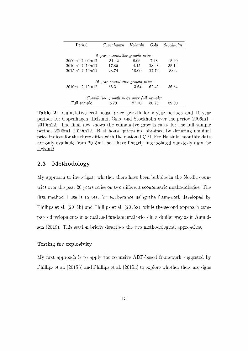
Period Copenhagen Helsinki Oslo Stockholm
5-year cumulative growth rates:
2006m1-2009m12 -31.42 9.06 7.48 18.492010m1-2014m12 17.86 4.15 28.48 38.142015m1-2019m12 28.74 10.00 22.73 8.06
10-year cumulative growth rates:
2010m1-2019m12 56.31 15.64 62.49 56.54
Cumulative growth rates over full sample:
Full sample 8.79 27.20 80.73 89.50
Table 2: Cumulative real house price growth for 5-year periods and 10-yearperiods for Copenhagen, Helsinki, Oslo, and Stockholm over the period 2006m1�2019m12. The �nal row shows the cumulative growth rates for the full sampleperiod, 2006m1�2019m12. Real house prices are obtained by de�ating nominalprice indices for the three cities with the national CPI. For Helsinki, monthly dataare only available from 2015m1, so I have linearly interpolated quarterly data forHelsinki.
2.3 Methodology
My approach to investigate whether there have been bubbles in the Nordic coun-
tries over the past 20 years relies on two di�erent econometric methodologies. The
�rst method I use is to test for exuberance using the framework developed by
Phillips et al. (2015b) and Phillips et al. (2015a), while the second approach com-
pares developments in actual and fundamental prices in a similar way as in Anund-
sen (2019). This section brie�y describes the two methodological approaches.
Testing for explosivity
My �rst approach is to apply the recursive ADF-based framework suggested by
Phillips et al. (2015b) and Phillips et al. (2015a) to explore whether there are signs
13
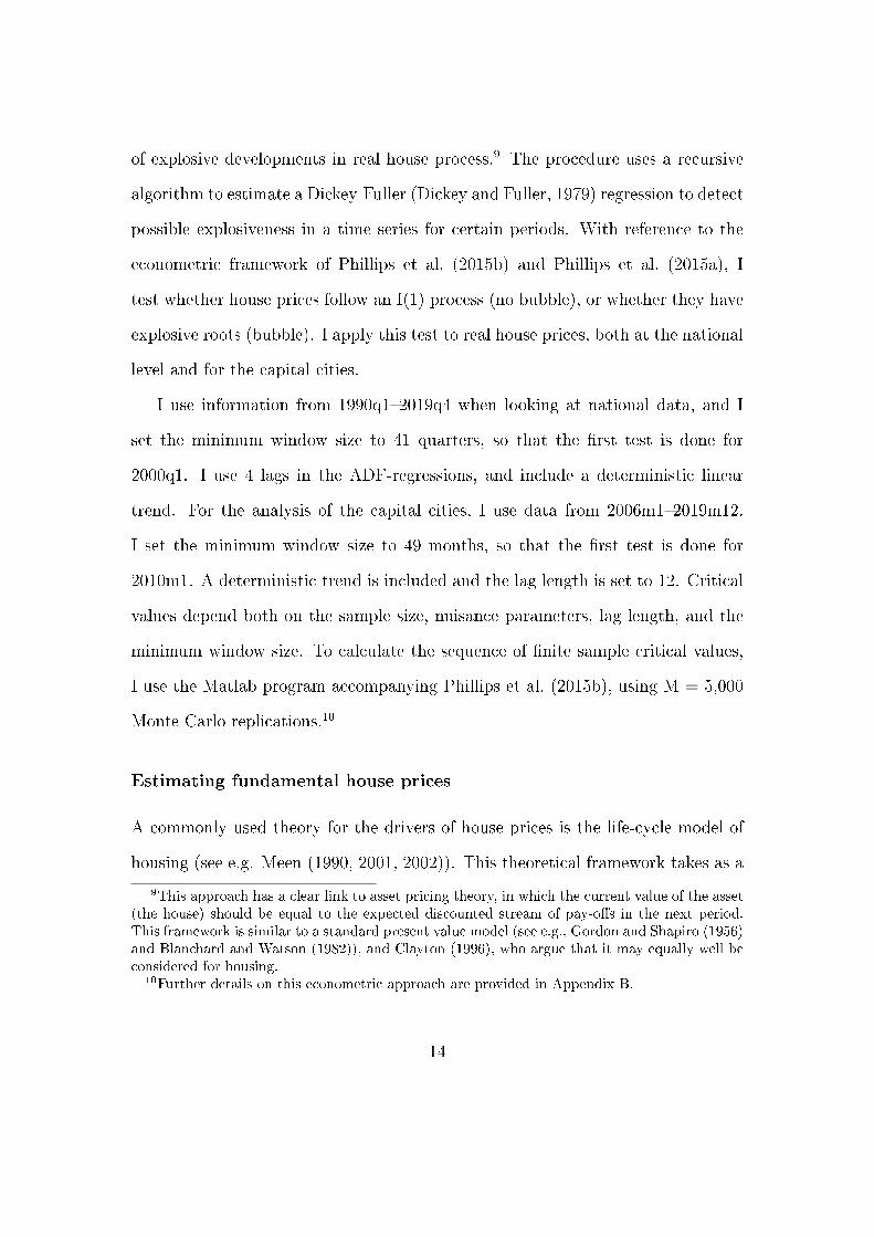
of explosive developments in real house process.9 The procedure uses a recursive
algorithm to estimate a Dickey-Fuller (Dickey and Fuller, 1979) regression to detect
possible explosiveness in a time series for certain periods. With reference to the
econometric framework of Phillips et al. (2015b) and Phillips et al. (2015a), I
test whether house prices follow an I(1) process (no bubble), or whether they have
explosive roots (bubble). I apply this test to real house prices, both at the national
level and for the capital cities.
I use information from 1990q1�2019q4 when looking at national data, and I
set the minimum window size to 41 quarters, so that the �rst test is done for
2000q1. I use 4 lags in the ADF-regressions, and include a deterministic linear
trend. For the analysis of the capital cities, I use data from 2006m1�2019m12.
I set the minimum window size to 49 months, so that the �rst test is done for
2010m1. A deterministic trend is included and the lag length is set to 12. Critical
values depend both on the sample size, nuisance parameters, lag length, and the
minimum window size. To calculate the sequence of �nite sample critical values,
I use the Matlab program accompanying Phillips et al. (2015b), using M = 5,000
Monte Carlo replications.10
Estimating fundamental house prices
A commonly used theory for the drivers of house prices is the life-cycle model of
housing (see e.g. Meen (1990, 2001, 2002)). This theoretical framework takes as a
9This approach has a clear link to asset pricing theory, in which the current value of the asset(the house) should be equal to the expected discounted stream of pay-o�s in the next period.This framework is similar to a standard present value model (see e.g., Gordon and Shapiro (1956)and Blanchard and Watson (1982)), and Clayton (1996), who argue that it may equally well beconsidered for housing.
10Further details on this econometric approach are provided in Appendix B.
14

starting point a standard representative-agent model, in which an agent maximizes
her lifetime utility with respect to consumption of housing goods and �other� goods.
One can show that this implies an inverted demand equation for housing, which has
been used in numerous studies that investigate house price determination (Buckley
and Ermisch, 1983; Hendry, 1984; Meen, 1990; Holly and Jones, 1997; Meen and
Andrew, 1998; Meen, 2001; Duca et al., 2011a,b; Anundsen, 2015). This inverted
demand equation implies that house prices are determined by income, the user
cost of housing, and the housing stock.
In my econometric operationalization, I start by applying the system-based test
for cointegration in Johansen (1988) to analyze the long-run relationship between
real house prices, real per capita income, the housing stock per capita, and the
real direct user cost (operationalized by considering real after-tax interest rates).
My estimation sample is 1985q1�1999q4 for Denmark, Norway, and Finland, while
the sample starts in 1990q1 for Sweden.11 The sample ends in 1999q4, so that
the parameters are determined before the evaluation period (2000q1�2019q4). To
save degrees of freedom, I impose the restriction that the coe�cient on income
and housing stock are the same, but with opposite signs. This implies an income
elasticity of demand equal to one, which is in accordance with what Meen (2001);
Duca et al. (2011b); Anundsen (2015) �nd on US data, and it is one of the cen-
tral estimates put out in Meen (2001).12 Detailed results from the cointegration
analysis are tabulated in Table B.1 in Appendix B.
Having obtained the parameters in the long-run relationships, I estimate the
implied fundamental house price path during the period 2000q1-2019q4. I as-
11For all countries, I consider a VAR(2)-model, which is also supported by Schwarz informationcriterion.
12A similar restriction is used in Anundsen (2019).
15

sume that house prices were in equilibrium in 2000q1, and I calculate the implied
fundamental trajectory of house prices in the ensuing period. Developments in
fundamental prices are then compared to actual house prices.13
3 Results
I start this section by looking at aggregate results for the Nordic countries. First,
I present my results from testing for exuberance, before I discuss the evolution of
house prices relative to what is implied by economic fundamentals. In the second
part, I test for periods of exuberance in the capital cities.
3.1 National results
Testing for explosive roots
The test statistics for all three countries are plotted together with critical values
for a 10% signi�cance level in Figure 3. The line for the critical values is plotted
in black, while the test statistic is shown in red. If the test statistic crosses the
black line, the test indicates that there are signs of exuberance.
It is evident that there are no points in time where the test statistic is higher
than the critical value for Finland, Norway, or Sweden. For Denmark, the test
indicates a bubble in the period before the sharp price drop starting in the �rst
quarter for 2007q1. There are no signs of bubble-behavior in Denmark in the
period thereafter.
13Further details on this econometric approach are provided in Appendix B.
16

-3-2
-10
12
2000
q1
2005
q1
2010
q1
2015
q1
2020
q1
Denmark No bubble
Denmark
-2-1
.5-1
-.50
.5
2000
q1
2005
q1
2010
q1
2015
q1
2020
q1
Finland No bubble
Finland
-4-3
-2-1
0
2000
q1
2005
q1
2010
q1
2015
q1
2020
q1
Norway No bubble
Norway
-2-1
01
2000
q1
2005
q1
2010
q1
2015
q1
2020
q1
Sweden No bubble
Sweden
Figure 3: Test for exuberance in Denmark, Finland, Norway, and Sweden.2000q1�2019q4. The �gure shows the test statistic for Denmark (upper left panel),Finland (upper right panel), Norway (lower left panel), and Sweden (lower rightpanel) based on the PSY-approach. The tests are performed on real house prices,which are obtained by de�ating the national house price indices by the nationalCPI. The test statistic is plotted in red, while the sequence of 10 percent criticalvalues are shown in black. The interpretation of the �gures is that if the test statis-tic crosses the black line, there are signs of exuberance. The sample covers theperiod 2000q1�2019q4 for all countries. The estimation sample starts in 1990q1. Iuse a minimum window size of 41 quarters, and include 4 lags and a deterministiclinear trend in the ADF-regressions. The critical values are simulated using 5000Monte Carlo replications. Details on the econometric approach are provided inAppendix B.
17

House prices and fundamentals
An important �nding from the cointegration analysis is that house prices are highly
sensitive to interest rate changes in all countries. This is particularly so in Denmark
and Norway, where my results suggest that an interest rate increase of one per-
centage point will lower long-run house prices by 13 and 11 percent, respectively.
The estimates for Norway resemble those in Anundsen (2019) and the estimates
for Denmark are close to Dam et al. (2011), in which similar type of models are
estimated. These estimates may be considered semi-elasticities of interest rates
on (equilibrium) house prices, and may have additional usage elsewhere for policy
makers.
The implied fundamental prices (orange) are plotted together with actual house
prices (black) in Figure 4, and average percentage deviations between actual and
fundamental prices are shown in Table 3.
Comparing actual to fundamental prices, it is evident that house prices were
overvalued in all four countries in the years leading up to the 2008 �nancial crisis.
The overvaluation was particularly prominent in Denmark, which also saw the
largest drop in actual house prices from peak-to-trough. This �nding is consistent
with the results from testing for exuberance, which points towards a bubble in the
Danish housing market in the years preceding the global �nancial crisis.
The correction in house prices around 2008, brought house prices back to the
value implied by fundamentals in all countries by 2010.
After 2010, Norwegian house prices remained undervalued, until 2016, in which
the model suggests that Norwegian house prices were overvalued. At the most,
prices were overvalued by 13 percent in 2018. Recently, prices have converged
18

Period Denmark Finland Norway Sweden
2000q1-2004q4 -2.82 6.57 1.62 -5.912005q1-2009q4 38.44 12.85 0.10 3.602010q1-2014q4 5.53 2.03 -4.58 -2.302015q1-2019q4 -5.34 3.72 2.15 7.39
Table 3: Average deviation from estimated fundamentals at the national levelfor 5-year periods from 2000q1 for Denmark, Finland, Norway, and Sweden. Realhouse prices are calculated by dividing the national indices by the national con-sumer price index. Fundamental prices are determined by income per capita, thehousing stock per capita, and real after tax interest rates. Detailed results onestimated coe�cients are given in Table B.1 in Appendix B.
back to their fundamental value, and at the end of 2019, prices were overvalued
by 9 percent.14 For Sweden, the estimates suggest that house prices have been
overvalued � although relatively modestly � since 2014. At the end of 2019, the
model suggests that Swedish house prices were overvalued by 7 percent.
In Finland, house prices have had a �at development since 2010, and prices have
been at, or even below, equilibrium in recent years. At the end of 2019, the model
suggests that Finnish house prices were undervalued by 3 percent. Following the
drop in house prices in the aftermath of the global �nancial crisis, Danish house
prices have remained mostly undervalued, and towards the end of the sample, my
estimates suggest that Danish house prices were undervalued by 9 percent.
Based on these results, I conclude that Danish and Finnish house prices were
undervalued at the end of 2019, whereas Norwegian and Swedish house prices were
overvalued. The only country where there are signs of systematic overvaluation is
Sweden, in which prices have remained elevated since 2014.
14Housing Lab � National center for housing market research updates this indicator for Norwayon a quarterly basis. Recent estimates suggest that the interest rate reduction accompanyingthe lock-down in relation to the spreading of Covid-19 has closed the gap between actual andfundamental prices � at the end of 2020q2, actual prices were a little less than one percent abovefundamentals, according to Housing Lab.
19

0.75
1.00
1.25
1.50
2000 2005 2010 2015 2020
Inde
x
Variable Actual prices Fundamental prices
Denmark
1.0
1.1
1.2
1.3
1.4
2000 2005 2010 2015 2020
Inde
x
Variable Actual prices Fundamental prices
Finland
0.8
1.2
1.6
2.0
2000 2005 2010 2015 2020
Inde
x
Variable Actual prices Fundamental prices
Norway
1.0
1.5
2.0
2.5
2000 2005 2010 2015 2020
Inde
x
Variable Actual prices Fundamental prices
Sweden
Figure 4: Actual versus fundamental house prices in Denmark, Finland, Norway,and Sweden. 2000q1�2019q4. The �gure shows fundamental house prices (orangeline) and actual house prices (black line) over the period 2000q1�2019q4 for Den-mark (upper left panel), Finland (upper right panel), Norway (lower left panel),and Sweden (lower right panel). Fundamental prices are determined by incomeper capita, the housing stock per capita, and real after tax interest rates. Bothfundamental and actual prices are normalized to one in 2000q1. Detailed resultson estimated coe�cients are given in Table B.1 in Appendix B.
3.2 Results for Copenhagen, Helsinki, Oslo, and Stockholm
Test statistics from the PSY-approach for Copenhagen, Helsinki, Oslo, and Stock-
holm are plotted together with critical values for a 10% signi�cance level in Figure
5. The line for the critical values is plotted in black. If the test statistic crosses
the black line, the test indicates that there are signs of exuberance. There are
no signs of exuberance in Helsinki over the sample period. There are some signs
20

of exuberance in Stockholm and Oslo, but this is very short-lived, so it is hard
to conclude that there has been bubble-like dynamics in these cities. For Copen-
hagen, there have been signs of exuberance between August 2018 and September
2019, but that there are no signs of exuberance towards the end of the sample.
21

-2-1
01
23
2010
m1
2012
m1
2014
m1
2016
m1
2018
m1
2020
m1
Copenhagen No bubble
Copenhagen
-3-2
-10
1
2010
m1
2012
m1
2014
m1
2016
m1
2018
m1
2020
m1
Helsinki No bubble
Helsinki
-4-2
02
4
2010
m1
2012
m1
2014
m1
2016
m1
2018
m1
2020
m1
Oslo No bubble
Oslo
-3-2
-10
12
2010
m1
2012
m1
2014
m1
2016
m1
2018
m1
2020
m1
Stocholm No bubble
Stockholm
Figure 5: Test for exuberance in Copenhagen, Helsinki, Oslo, and Stockholm.2006m1�2019m12. The �gure shows test statistics for Copenhagen (upper leftpanel), Helsinki (upper right panel), Oslo (lower left panel), and Stockholm (lowerright panel) from the PSY-approach. The tests are done on real house prices, whichare obtained by de�ating the city-level house price indices by the national CPI.The test statistic is plotted in red, while the sequence of 10 percent critical valuesare shown in black. The interpretation of the �gures is that if the test statisticcrosses the black line, there are signs of exuberance. The sample covers the period2010m1�2019m12 for all cities. The estimation sample starts in 2006m1. I use aminimum window size of 49 months, and include 12 lags and a deterministic lineartrend in the ADF-regressions. The critical values are simulated using 5000 MonteCarlo replications. Details on the econometric approach are provided in AppendixB.
22

4 What factors contribute to overvaluation?
My results indicate that the Nordic housing markets are sensitive to interest rate
changes. In order to probe deeper into this �nding, I have estimated quasi-
counterfactual developments for fundamental prices, by holding the real after-tax
interest rate �xed since 2000q1. This is not a fully-�edged counterfactual analy-
sis, however, since that would require a model taking general equilibrium e�ects
into account. The main motivation for this analysis is simply to illustrate the
importance of developments in the real after-tax interest rate for the evolution of
fundamental house prices.
In Figure 6, I plot actual house prices (solid black), fundamental house prices
(orange), and fundamental house prices when holding the real after-tax interest
rate constant from 2000q1 (blue). It is evident that the real after-tax interest rate
matters a great deal to fundamental prices. At face value, this exercise suggest
that house prices would have been greatly overvalued in all countries over large
parts of the sample period had it not been for the secular decline in the real after-
tax interest rate. Of course, this is a simpli�cation, since another development
in the real after-tax interest rate also would have a�ected the other fundamentals
in the model, and it would have resulted in another development in actual house
prices.
That interest rate developments are important to house price dynamics �nds
support in the literature, see e.g., Williams (2015) for an excellent summary of
some international studies. For US metro areas, Aastveit and Anundsen (2017)
show that monetary policy shocks exercise a great impact on house price develop-
ments. They also show that whether expansionary or contractionary shocks have
23

0.75
1.00
1.25
1.50
2000 2005 2010 2015 2020
Inde
x
Variable Actual prices Constant user cost Fundamental prices
Denmark
1.0
1.1
1.2
1.3
1.4
2000 2005 2010 2015 2020
Inde
x
Variable Actual prices Constant user cost Fundamental prices
Finland
0.8
1.2
1.6
2.0
2000 2005 2010 2015 2020
Inde
x
Variable Actual prices Constant user cost Fundamental prices
Norway
1.0
1.5
2.0
2.5
2000 2005 2010 2015 2020
Inde
x
Variable Actual prices Constant user cost Fundamental prices
Sweden
Figure 6: Fundamental house prices, actual house prices, and fundamental houseprices without interest rate changes. Denmark, Finland, Norway, and Sweden.2000q1�2019q4. The �gure shows fundamental house prices (orange line), actualhouse prices (black line) and fundamental prices when the interest rate is keptunchanged from 2000q1 for Finland (upper left panel), Denmark (upper rightpanel), Norway (lower left panel), and Sweden (lower right panel). The samplecovers the period 2000q1�2019q4. Fundamental prices are determined by incomeper capita, the housing stock per capita, and real interest rates after taxes. Allseries are normalized to one in 2000q1. Detailed results on estimated coe�cientsare given in Table B.1 in Appendix B.
the greatest impact on house prices depends on the elasticity of housing supply.
In particular, they show that expansionary shocks have a greater impact on house
prices in areas with low housing supply elasticities, whereas the opposite is true
for areas with high housing supply elasticities. At the median, they �nd that
expansionary shocks hit harder than contractionary shocks.
24

The average housing supply elasticity in the US is calculated to be around 2
(Caldera and Johansson, 2013).15 The estimated elasticities in Caldera and Jo-
hansson (2013) for Denmark (1.2), Finland (less than 1), Norway (0.5), and Sweden
(1.4) are all estimated to be lower than in the US. To the extent that the results
in Aastveit and Anundsen (2017) are generalizable outside the US, contractionary
monetary policy may have a relatively weaker impact in slowing down house price
increases than expansionary shocks have in fuelling price increases. This can cre-
ate a trade-o� for �nancial stability purposes, as expansionary shocks fuels house
price increases, whereas the reduction in house prices is more modest following a
corresponding increase in the interest rate.
House prices are autocorrelated (Case and Shiller (1989); Cutler et al. (1991);
Røed Larsen and Weum (2008); Head et al. (2014)), and momentum e�ects are
seen as a key feature of the housing market (Glaeser et al., 2014). Aastveit and
Anundsen (2017) suggest that one potential reason for why expansionary monetary
policy shocks have a greater impact on house prices than contractionary shocks is
that momentum e�ects are asymmetric. For instance, if an interest rate reduction
increases house prices, a momentum e�ect may lead to an additional increase in
demand. This increases house prices further. Such a momentum e�ect is more
important in supply inelastic markets, since the initial price increase is greater.
On the other hand, an interest rate increase typically leads to lower house prices.
If the momentum e�ect is less prominent when prices are falling, the additional
demand increase will also be smaller. Aastveit and Anundsen (2017) show that
the coe�cients on lagged house prices in a simple AR(4)-model for a panel of 263
15This estimate is close to the average estimate in Saiz (2010), who construct estimates ofsupply elasticities for US metro areas. It is the elasticities in Saiz (2010) that are used byAastveit and Anundsen (2017).
25

MSAs are twice as large when house prices are increasing.
To explore the relevance of asymmetric momentum e�ects in the Nordic housing
markets, I have estimated simple AR(4)-models for house price growth, where I
follow Aastveit and Anundsen (2017) and let the AR-coe�cients be di�erent in
periods when the four-quarter growth in real house prices is positive versus periods
when the four-quarter growth is negative. I have estimated these models for each
country separately, and pooled as a panel using a �xed-e�ects estimator. Results
are listed in Table 4. Results are consistent with Aastveit and Anundsen (2017) and
suggest that the momentum e�ect is more pronounced when prices are increasing.
In sum, the results from the simple AR-models and the low supply elasticities
estimated for Nordic countries (Caldera and Johansson, 2013) are consistent with
the idea that expansionary shocks have a greater impact on house prices than
contractionary shocks.
Low supply elasticities are also shown to increase house price volatility in booms
and busts Huang and Tang (2012); Glaeser et al. (2008); Anundsen and Heebøll
(2016)), and � with the low supply elasticities in the Nordic countries � one may
be worried that prices may take a hit in the future. From a policy point of view,
fewer restrictions on construction activity would make builders more responsive
to house price increases, thereby dampening the e�ects of demand shocks and
lowering house price volatility over the course of a boom-bust cycle. Policy actions
that could reduce the bureaucratic hurdle in the building process could therefore
lower the chances of bubbles building up. If there is a supply side problem, it is
easier to solve it on the supply side, not by manipulation of the demand side.
Several papers have also shown that relaxation of lending standards matters to
regional house price developments in the US (e.g., Mian and Su� (2009); Favara
26

Country Pos. Coe� Pos. SE Neg. Coe�. Neg. SE
Denmark 0.84 0.12 0.79 0.14Finland 0.92 0.20 -0.14 0.33Norway 0.64 0.22 0.33 0.41Sweden 0.84 0.20 -0.47 0.48Panel 0.79 0.10 0.47 0.14
Table 4: Momentum e�ects. The table reports the sum of coe�cients on laggedhouse price appreciation based on estimating an AR(4)-model for house pricegrowth, where the coe�cients on lagged house prices are allowed to be di�er-ent when the four-quarter growth is positive versus negative. Results are shownfor each individual country, and when the countries are pooled as a panel (�nalrow). I include country-�xed e�ects in the panel estimation.
and Imbs (2015); Anundsen and Heebøll (2016)), and a strand of the literature
attributes the bubble-like dynamics in the US housing market in the 2000s to
the subprime explosion (see Duca et al. (2011a,b); Pavlov and Wachter (2011);
Anundsen (2015)). In this context, it may be tempting for authorities to impose
limits to credit expansion through macroprudential policies. As a policy to cool
down credit growth and to lower the risk of �nancial imbalances, this may be
a sound tool, but it is not necesarrily the best way to deal with housing market
developments. If the reason why prices are increasing is that not enough houses are
built in high-demand areas, it is a supply-side problem that requires supply-side
policies. Tightening of credit standards can lower credit growth and thereby lower
demand for housing. This pushes house prices down, but at the same time results
in less construction activity � thus magnifying the initial structural de�ciency.
Given the low elasticities that are estimated for the Nordic countries, together
with the high interest rate sensitivity, it seems to be of acute importance that one
commissions a thorough investigation of political hurdles in the building process,
which also studies housing needs in di�erent part of the countries, and in particular
whether new construction activity meets the actual needs in terms of type of
27

housing, size, and not least location.
5 Conclusion
In this paper, I have investigated whether there are signs of bubbles in the Danish,
Finnish, Norwegian, and Swedish housing markets. First, I tested for explosive
developments in real house prices. My results suggest that Danish house prices had
an explosive development in the years preceding the global �nancial crisis. There
is no evidence of explosiveness for the other Nordic countries. I also estimated the
trajectory of fundamental house prices for the period 2000q1-2019q4, as implied
by developments in per capita income, the housing stock per capita, and the real
after-tax interest rate. My results show that there were signs of overvaluation in
all countries before the housing busts towards the end of the previous decade. In
2019, I �nd that Norwegian and Swedish house prices were overvalued, and that
they have been so in Sweden since 2014. My results show that Danish and Finnish
house prices were undervalued at the end of 2019.
My estimation results imply that the Nordic housing markets are highly sensi-
tive to interest rate changes, and that the secular decline in real after-tax interest
rates over the past 20 years has been a major contributor to developments in fun-
damental house prices. A quasi-counterfactual exercise suggest that house prices
would have been grossly overvalued for most part of the sample in all counties if
the real after-tax interest rate had been kept constant since 2000. I argue that the
high sensitivity of house prices with respect to interest rate changes in Denmark,
Finland, Norway, and Sweden must be seen in conjunction with the low housing
supply elasticities that have been estimated for the Nordic countries. The low elas-
28

ticities contribute to increased house price volatility over the boom-bust cycle and
implies a stronger e�ect of demand shocks on house prices. In conclusion, I think
it is of key importance that policy makers in the Nordic countries gets a thorough
overview of housing needs in terms of geographical preferences, as well as latent
demand for size and type of units, so that new construction meets these needs.
Removing bureaucratic hurdles in the building process can also lower house prices
in the long run, make them less sensitive to demand shocks and reduce house price
volatility.
29

References
Aastveit, K. A. and A. K. Anundsen (2017). Asymmetric e�ects of monetary policy
in regional housing markets. Working Paper 25, Norges Bank.
Aastveit, K. A., A. K. Anundsen, and E. I. Herstad (2019). Residential investment
and recession predictability. International Journal of Forecasting 35 (4), 1790�
1799.
Amador-Torres, J. S., J. E. Gomez-Gonzalez, and S. Sanin-Restrepo (2018). De-
terminants of housing bubbles' duration in OECD countries. International Fi-
nance 21 (2), 140�157.
Anundsen, A. K. (2015). Econometric regime shifts and the US subprime bubble.
Journal of Applied Econometrics 30 (1), 145�169.
Anundsen, A. K. (2019). Detecting imbalances in house prices: What goes up
must come down? Scandinavian Journal of Economics 121 (4), 1587�1619.
Anundsen, A. K., K. Gerdrup, F. Hansen, and K. Kragh-Sørensen (2016). Bubbles
and crises: The role of house prices and credit. Journal of Applied Economet-
rics 31 (7), 1291�1311.
Anundsen, A. K. and C. Heebøll (2016). Supply restrictions, subprime lending and
regional US housing prices. Journal of Housing Economics 31, 54�72.
Anundsen, A. K. and E. S. Jansen (2013). Self-reinforcing e�ects between housing
prices and credit. Journal of Housing Economics 22 (3), 192�212.
30

Aron, J., J. V. Duca, J. Muellbauer, K. Murata, and A. Murphy (2012). Credit,
housing collateral and consumption: Evidence from the UK, Japan and the US.
Review of Income and Wealth 58 (3), 397�423.
Bergman, U. M. and P. B. Sørensen (2018). The interaction of actual and funda-
mental house prices: A general model with an application to Sweden. Unpub-
lished manuscript.
Blanchard, O. and M. Watson (1982). Crisis in the Economics Financial Structure.
Lexington Books, Lexington.
Brown, J. and D. A. Matsa (2020). Locked in by leverage: Job search during the
housing crisis. Journal of Financial Economics 136 (3), 623�648.
Buckley, R. and J. Ermisch (1983). Theory and empiricism in the econometric
modelling of house prices. Urban Studies 20 (1), 83�90.
Caldera, A. and Å. Johansson (2013). The price responsiveness of housing supply
in OECD countries. Journal of Housing Economics 22 (3), 231�249.
Capozza, D. R., P. H. Hendershott, and C. Mack (2004). An anatomy of price
dynamics in illiquid markets: analysis and evidence from local markets. Real
Estate Economics 32 (1), 1�32.
Case, K. E. and R. J. Shiller (1989). The e�ciency of the market for single-family
homes. American Economic Review 79 (1), 125�137.
Caspi, I. (2016). Testing for a housing bubble at the national and regional level:
The case of Israel. Empirical Economics 51, 483�516.
31

Clayton, J. (1996). Rational expectations, market fundamentals and housing price
volatility. Real Estate Economics 24 (4), 441�470.
Commission, E. (2013). Finland's high house prices and household debt: A source
of concern. Country Focus 6, European Commission.
Cutler, D. M., J. M. Poterba, and L. H. Summers (1991). Speculative dynamics.
Review of Economic Studies 58 (3), 529�546.
Dam, N. A., T. S. Hvolbøl, E. H. Pedersen, P. B. Sørensen, and S. H. Thamsborg
(2011). Udviklingen på ejerboligmarkedet i de senere år - Kan boligpriserne
forklares? (Developments in the housing market in recent years - Can the price
developments be explained?). Kvartalsoversigt 2011-2, Nationalbanken.
Dermani, E., J. Lindé, and K. Walentin (2016). Is there an evident housing bubble
in Sweden? Economic review, Sveriges Riksbank.
Dickey, D. A. and W. A. Fuller (1979). Distribution of the estimators for au-
toregressive time series with a unit root. Journal of the American Statistical
Association 74 (366), 427�431.
Duca, J., Muellbauer, J., and A. Murphy (2020). What drives house price cycles?
international experience and policy issues. Journal of Economic Literature.
Forthcoming.
Duca, J., J. Muellbauer, and A. Murphy (2011a). House prices and credit con-
straints: Making sense of the US experience. Economic Journal 121, 533�551.
Duca, J., J. Muellbauer, and A. Murphy (2011b). Shifting credit standards and
32

the boom and bust in US home prices. Technical Report 1104, Federal Reserve
Bank of Dallas.
Duca, J. V. (2020). Making sense of increased synchronization in global house
prices. Journal of European Real Estate Research.
Favara, G. and J. Imbs (2015, March). Credit Supply and the Price of Housing.
American Economic Review 105 (3), 958�92.
Ferreira, F. and J. Gyourko (2012). Heterogeneity in neighborhood-level price
growth in the United States, 1993-2009. American Economic Review 102 (3),
134�140.
Ferreira, F., J. Gyourko, and J. Tracy (2010). Housing burst and household mo-
bility. Journal of Urban Economics 68, 34�45.
Fitzpatrick, T. and K. McQuinn (2007). House prices and mortgage credit: Em-
pirical evidence for Ireland. The Manchester School 75, 82�103.
Geng, N. (2018). Fundamental drivers of house prices in advanced economies. IMF
Working Paper 18/164, IMF.
Gimeno, R. and C. Martinez-Carrascal (2010). The relationship between house
prices and house purchase loans: The Spanish case. Journal of Banking and
Finance 34, 1849�1855.
Glaeser, E., J. Gyourko, E. Morales, and C. G. Nathanson (2014). Housing dy-
namics: An urban approach. Journal of Urban Economics 81, 45�56.
Glaeser, E., J. Gyourko, and A. Saiz (2008). Housing supply and housing bubbles.
Journal of Urban Economics 64 (2), 198�217.
33

Gomez-Gonzalez, J., J. Gamboa-Arbelàez, J. Hirs-Garzòn, and A. Pinchao Rosero
(2018). When bubble meets bubble: Contagion in oecd countries. Journal of
Real Estate Finanance and Econonmics 56, 546�566.
Gordon, M. J. and E. Shapiro (1956). Capital equipment analysis: The required
rate of pro�t. Management Science 3 (1), 102�110.
Head, A., H. Lloyd-Ellis, and S. Hongfei (2014). Search, liquidity, and the dynamics
of house prices and construction. American Economic Review 104 (4), 1172�
1210.
Hendry, D. F. (1984). Econometric modelling of house prices in the United King-
dom. In D. F. Hendry and K. F. Wallis (Eds.), Econometrics and Quantitative
Econometrics, Chapter 8, pp. 211�252. Blackwell.
Hofmann, B. (2003). Bank lending and property prices: Some international evi-
dence. Working paper 22, The Hong Kong Institute for Monetary Research.
Holly, S. and N. Jones (1997). House prices since the 1940s: Cointegration, de-
mography and asymmetries. Economic Modelling 14 (4), 549�565.
Huang, H. and Y. Tang (2012). Residential land use regulation and the US housing
price cycle between 2000 and 2009. Journal of Urban Economics 71 (1), 93�99.
IMF (2019a). Finland. Country Report 5, International Monetary Fund.
IMF (2019b). Norway. Country Report 159, International Monetary Fund.
IMF (2019c). Sweden. Country Report 88, International Monetary Fund.
34

Johansen, S. (1988). Statistical analysis of cointegration vectors. Journal of Eco-
nomic Dynamics and Control 12, 231�254.
Leamer, E. E. (2007). Housing IS the business cycle. In Housing, Housing Finance,
and Monetary Policy, pp. 149�233. Federal Reserve Bank of Kansas City.
Leamer, E. E. (2015). Housing really is the business cycle: What survives the
lessons of 2008-09? Journal of Money, Credit and Banking 47 (1), 43�50.
Malpezzi, S. and S. Wachter (2005). The role of speculation in real estate cycles.
Journal of Real Estate Literature 13 (2), 143�164.
Meen, G. (1990). The removal of mortgage market constraints and the implications
for econometric modelling of UK house prices. Oxford Bulletin of Economics and
Statistics 52 (1), 1�23.
Meen, G. (2001). Modelling Spatial Housing Markets: Theory, Analysis and Policy.
Kluwer Academic Publishers, Boston.
Meen, G. (2002). The time-series behavior of house prices: A transatlantic divide?
Journal of Housing Economics 11 (1), 1�23.
Meen, G. and M. Andrew (1998). On the aggregate housing market implications
of labour market change. Scottish Journal of Political Economy 45 (4), 393�419.
Mian, A., K. Rao, and A. Su� (2013). Household balance sheets, consumption,
and the economic slump. Quarterly Journal of Economics 128 (4), 1687�1726.
Mian, A. and A. Su� (2009). The consequences of mortgage credit expansion:
Evidence from the U.S. mortgage default crisis. Quarterly Journal of Eco-
nomics 124 (4), 1449�1496.
35

Mian, A. and A. Su� (2014). What explains the 2007-2009 drop in employment?
Econometrica 82 (6), 2197�2223.
Moodys (2017). High house prices pose persistent risk where slow to adjust to
homeownership costs. Sector in-depth December, Moody's.
Pavlov, A. and S. Wachter (2011). Subprime lending and real estate prices. Real
Estate Economics 39 (1), 1�17.
Phillips, P. C. B. and S. Shi (2019). Detecting �nancial collapse and ballooning
sovereign risk. Oxford Bulletin of Economics and Statistics 81 (6), 1336�1361.
Phillips, P. C. B. and S. Shi (2020). Chapter 2 - real time monitoring of asset
markets: Bubbles and crises. In D. V. Hrishikesh and C. Rao (Eds.), Financial,
Macro and Micro Econometrics Using R, Volume 42 of Handbook of Statistics,
pp. 61�80. Elsevier.
Phillips, P. C. B., S. P. Shi, and J. Yu (2015a). Testing for multiple bubbles:
Historical episodes of exuberance and collapse in the S&P 500. International
Economic Review 56 (4), 1043�1078.
Phillips, P. C. B., S. P. Shi, and J. Yu (2015b). Testing for multiple bubbles:
Limit theory and real time detectors. International Economic Review 56 (4),
1079�1134.
Røed Larsen, E. and S. Weum (2008). Testing the e�ciency of the Norwegian
housing market. Journal of Urban Economics 64 (2), 510�517.
Saiz, A. (2010). The geographic determinants of housing supply. Quarterly Journal
of Economics 125 (3), 1253�1296.
36

Stiglitz, J. E. (1990). Symposium on bubbles. Journal of Economic Perspec-
tives 4 (2), 13�18.
Williams, J. C. (2015). Measuring monetary policy's e�ect on house prices. FRBSF
Economic Letter (28).
Yiu, M. and L. Jin (2013). Detecting bubbles in the hong kong residential property
market: An explosive-pattern approach. Journal of Asian Economics 28, 115�
124.
37

A Data de�nitions
Series Description Denmark Finland Norway Sweden
PH House price index DS/DN SF/BoF SSB/NB/EV SS/RB/VGP Consumer Price Index DS SF/BoF SSB/NB SS/RBH Housing stock DS/DN SF/BoF SSB/NB SS/RBY Households' disposable income DS/DN SF/BoF SSB/NB SS/RBi Mortgage interest rate RKR/DN/Dam et al. (2011) BoF NB RBτy Capital gains tax rate DS BoF SSB/NB RBPOP Population DS/DN SF/BoF SSB/NB SS/RB
Table A.1: Variable de�nitions and data sources. The data period runs from1985q1 to 2019q4 for Denmark, Finland, and Norway. For Sweden, the samplecovers the the period 1909q1�2019q4. The abbreviations are the following: SD =Danmarks Statistikk, DN = Danmarks Nationalbank, RKR = Realkredittrådet,SF = Statistics Finland, BoF = Bank of Finland, SSB = Statistisk Sentralbyrå,NB = Norges Bank, EV = Eiendomsverdi, SCB = Statistiska Centralbyrån, RB= Riksbanken, and VG = Valueguard. For Denmark, I follow Dam et al. (2011)and construct the real after-tax interest rate using a combination of the interestrate on 30-year bonds and 1-year bonds, controlling for the minimum amortizationrate and property taxes.
38

B Methodology
Exuberance
Below is a brief explanation of the recursive ADF-based framework of Phillips
et al. (2015b,a). Consider the following generalized ADF-regression model:
∆Xt = µr1,r2 + ρr1,r2Xt−1 +
p∑j=1
γr1,r2∆Xt−j + εt, εt ∼ IIN(0, σ2r1,r2
)
where r1 = T1T
and r2 = T2T, with T1, T2 and T denoting the sample starting
point, end point and the total number of observations, respectively. When T1 = 0
and T2 = T , the model is similar to a standard ADF-regression model. The null
hypothesis of interest is that ρr1,r2 = 0, i.e., that Xt ∼ I(1) versus the alternative
hypothesis that ρr1,r2 > 0, i.e., that Xt is explosive. The test statistic is computed
as ADF r2r1
=ρ̂i,r1,r2
se(ρ̂i,r1,r2). Like standard ADF test statistics, this test statistic has
a non-standard limiting distribution under the null hypothesis. Moreover, the
distribution depends on both r2 and nuisance parameters. Finite sample critical
values may be simulated using a Monte Carlo simulation.
My aim is to identify whether there are signs of explosive house price develop-
ments at di�erent points in time. I test this by applying the Backward Sup ADF
(BSADF) test of Phillips et al. (2015b,a). Consider the case where we keep the
sample end point �xed at T̄2. The BSADF-statistic then becomes:
BADF (r2 = r̄2) = supr1∈[0,r̄2−r̃]
ADF r2=r̄2r1
where r̃ = T̃T, in which T̃ is the minimum sample used for the test. By recursively
39
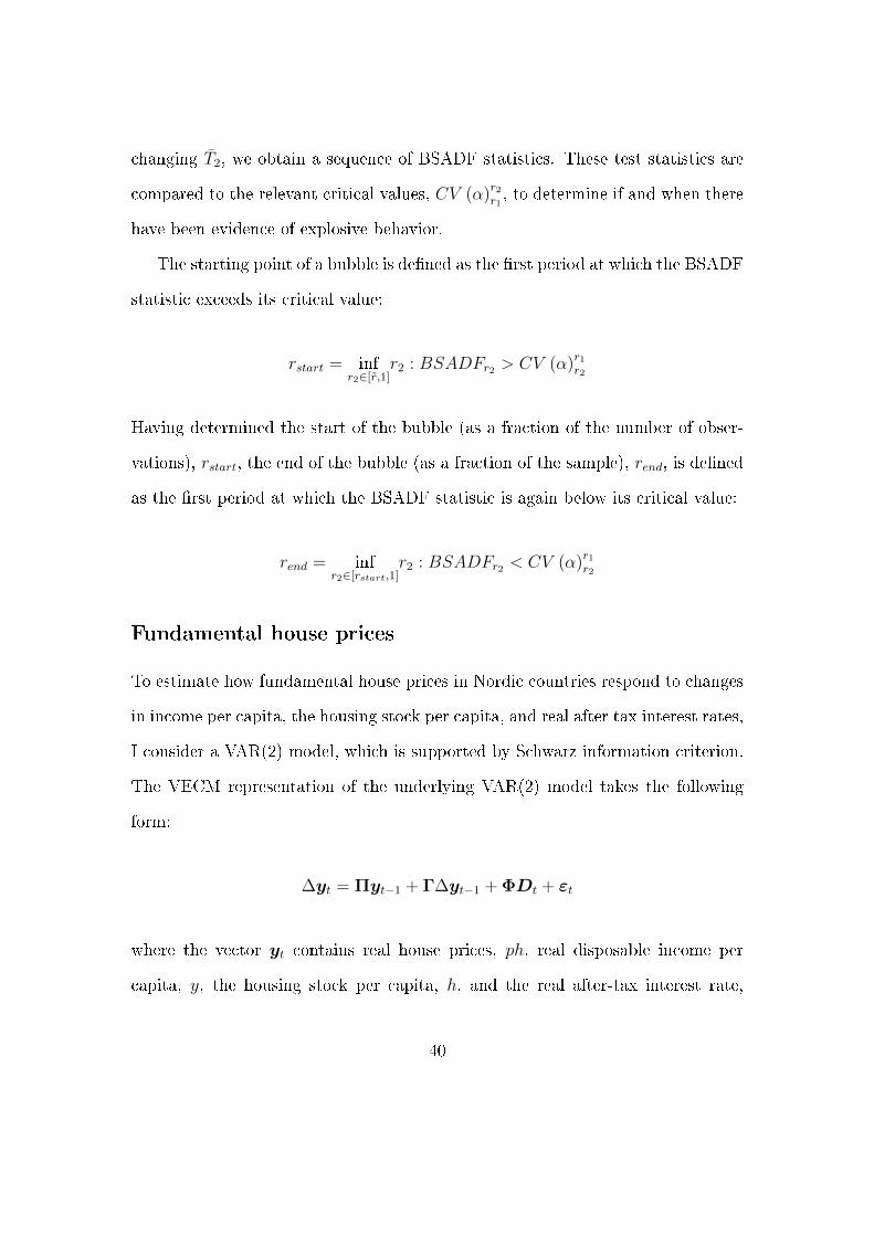
changing T̄2, we obtain a sequence of BSADF statistics. These test statistics are
compared to the relevant critical values, CV (α)r2r1 , to determine if and when there
have been evidence of explosive behavior.
The starting point of a bubble is de�ned as the �rst period at which the BSADF
statistic exceeds its critical value:
rstart = infr2∈[r̃,1]
r2 : BSADFr2 > CV (α)r1r2
Having determined the start of the bubble (as a fraction of the number of obser-
vations), rstart, the end of the bubble (as a fraction of the sample), rend, is de�ned
as the �rst period at which the BSADF statistic is again below its critical value:
rend = infr2∈[rstart,1]
r2 : BSADFr2 < CV (α)r1r2
Fundamental house prices
To estimate how fundamental house prices in Nordic countries respond to changes
in income per capita, the housing stock per capita, and real after tax interest rates,
I consider a VAR(2) model, which is supported by Schwarz information criterion.
The VECM representation of the underlying VAR(2) model takes the following
form:
∆yt = Πyt−1 + Γ∆yt−1 + ΦDt + εt
where the vector yt contains real house prices, ph, real disposable income per
capita, y, the housing stock per capita, h, and the real after-tax interest rate,
40

r. The vector D collects a constant, and a deterministic trend. I impose the
restriction that the coe�cient on income and housing stock are the same, but with
opposite signs, so that the vector yt is 3 × 1. This restriction implies an income
elasticity of demand equal to one, which is in accordance with what Meen (2001);
Duca et al. (2011b); Anundsen (2015) �nd on US data, and it is one of the central
estimates put out in Meen (2001).16 The disturbances are assumed to follow a
multivariate normal distribution, εt ∼MVN (0,Σ).
Testing for cointegration amounts to testing the rank of the matrix Π, which
corresponds to the number of independent linear combinations of the variables in
yt that are stationary. I test this using the trace test and impose Rank (Π) = 1.
The reduced rank representation implies that Π = αβ′, where α is a 3×1 matrix,
whereas β is a 4× 1 matrix (since a deterministic trend is also restricted to enter
the space spanned by α). Having imposed a rank of one, I follow Anundsen
(2019) and impose the restrictions that the series in yt are co-trending, and that
disposable per capita income relative to the existing housing stock per capita and
the real after-tax interest rate are weakly exogenous with respect to the long-run
parameters. Table B.1 summarizes the estimated long-run coe�cients, β, and the
adjustment parameter, αph, for each of the countries.
It is evident that there is a substantial interest rate e�ect in all countries,
and that the income e�ect is larger in Norway and Denmark than in Sweden and
Finland. There is also evidence suggesting that equilibrium deviations are restored
more slowly in Norway and Denmark than in the other two countries.
Having determined the parameters in the long-run relationship, I construct the
16A similar restriction is used in Anundsen (2019).
41

Variable Denmark Finland Norway Sweden
Real interest rate -12.548 -7.902 -11.001 -5.842(6.389) (0.986) (5.106) (1.495)
Disp. income 4.775 0.959 5.362 2.153(1.667) (0.481) (1.327) (1.360)
Housing stock -4.775 -0.959 -5.362 -2.153(-) (-) (-) (-)
Adjustment parameter -0.045 -0.191 -0.029 -0.146(0.016) (0.058) (0.006) (0.043)
Table B.1: Results from cointegration analysis. This table reports a summaryof the main results when the system based approach of Johansen (1988) is imple-mented. The estimation period runs from 1985q1 to 1999q4 for Denmark, Finland,and Norway. For Sweden, it covers the period 1990q1�1999q4. The dependentvariable is real house prices, while the independent variables are real per capitadisposable income, the housing stock per capita, and the real after tax interestrate. The VAR models are of order two.
fundamental house price path in the following way:
ph∗t = ph∗t−1 + β̂1999q4y ∆yt + β̂1999q4
h ∆ht + β̂1999q4r ∆rt ; t > 1999q4
42

Acknowledgements:
Housing Lab is partly funded by the Norwegian Ministry of Finance and the Norwegian
Ministry of Modernisation and Municipalities. Housing Lab also receives �nancial
support from Krogsveen and Sparebank1-Gruppen. We are greatful for the �nancial
support. All views expressed in our papers are the sole responsibility of Housing Lab,
and does not necessarily represent the views of our sponsors. The authors are grateful
to DNB Eiendom and Eiendomsverdi for auction and transaction data.
Authors:
André K. Anundsen, Housing Lab, Oslo Metropolitan University, Norway;
email: [email protected]
ISSN: 2703-786X (Online)