HOMES No. 6

Household Projections and Housing Needs in Thailand

Nipon Poapongsakorn

June 1988

EAST-WEST P O P U L A T I O N INSTITUTE

EAST-WEST CENTER [jt] H O N O L U L U , HAWAII

HOMES Research Reports are circulated to inform planners and researchers about research findings and training materials from the Household Model for Economic and Social Studies devel­oped at the East-West Population Institute. The primary purpose of the HOMES project is to expand the scope and improve the quality of demographic information available for development planning and the formulation of economic and social policy by providing projections of the number and demographic charac­teristics of households. In addit ion, modules have been devel­oped to forecast economic changes in the household sector, for example in the composit ion of consumer expenditures, labor supply, and aggregate household saving. The HOMES project has been supported by the U.S. Agency for International Develop­ment, the Asian Development Bank, and the General Motors Research Laboratories. Their support is gratefully acknowledged. A list of other HOMES publications is included with this report. For further information about HOMES please contact: Andrew Mason, East-West Population Institute, East-West Center, Honolu lu , Hawaii 96848.

HOMES Research Report

No. 6

Household Projections and Housing Needs in Thailand

Nipon Poapongsakorn

June 1988

East-West Population Institute East-West Center

1777 East West Road Honolulu, Hawaii 96848

i i i

This report was prepared for the Asian Development Bank as part of the Technical Assistance to Thailand for the Demographic and Economic Forecasting Pilot Study in Cooperation with the National Economic and Social Development Board.

1

Household Projections and Housing Needs in Thailand

I . Introduction

The National Economic and Social Development Board in Thailand

has prepared several population projections up to year 2005. However,

household projection has never been prepared in Thailand. Household

projection is usually done in connection with forecasting demand for

housing or housing need in a country because the demographic factors

are perhaps ones or the most, i f not the most, determinants or residential

construction and residential building cycle.* Previous research, par t i ­

cularly i n the United States, have shown that residential construction

has a close inverse relationship with economic growth and fluctuations.

As a result of demographic, transition where total f e r t i l i t y

rate has rapidly declined from the high level i n the 1960fs to a low

level in the late 1970's, the Thai housing population, composed of

persons f i f t een years and older has drastically increased and w i l l

continue to increase in the rest of the century. This suggests that

Thailand w i l l experience an unparalleled increase in housing demand

between now and the year 2015 which w i l l put pressure on the construction

industry resources. Information about underlying change in housing

demand w i l l be necessary for government policies and the private sector

to appropriately direct investment and resources i n the construction

industry.

2

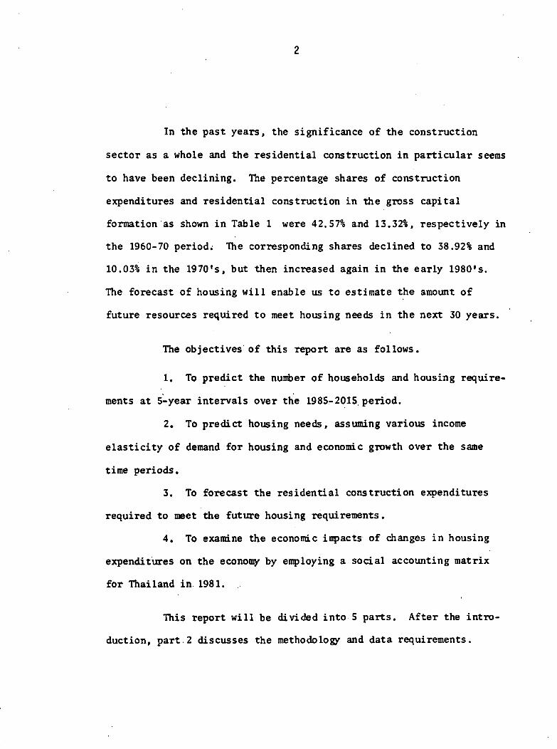
In the past years, the significance of the construction

sector as a whole and the residential construction in particular seems

to have been declining. The percentage shares of construction

expenditures and residential construction in the gross capital

formation as shown in Table 1 were 42,57% and 13.32%, respectively in

the 1960-70 period. The corresponding shares declined to 38.92% and

10.03% in the 1970's, but then increased again in the early 1980 ,s.

The forecast of housing w i l l enable us to estimate the amount of

future resources required to meet housing needs i n the next 30 years.

The objectives of this report are as follows.

1. To predict the number of households and housing require­

ments at 5-year intervals over the 1985-2015 period.

2. To predict housing needs, assuming various income

e las t i c i ty of demand for housing and economic growth over the same

time periods.

3. To forecast the residential construction expenditures

required to meet the future housing requirements.

4. To examine the economic impacts of changes i n housing

expenditures on the economy by employing a social accounting matrix

for Thailand in 1981.

This report w i l l be divided into 5 parts. After the intro­

duction, part 2 discusses the methodology and data requirements.

3

Projections of number of households, housing starts and residential

construction expenditures are presented in part 3. Part 4 describes

the construction sector i n Thailand and the economic impacts of

increase in residential construction expenditures i n the future. Part

5 is a summary and conclusion.

2. Methodology and Data Requirements

We w i l l f i r s t discuss the projection method of the number of

households. Then a method to estimate the number of housing starts

and residential construction expenditure w i l l be presented. F ina l ly ,

we w i l l b r i e f ly discuss the methods to assess economic impacts of

changes in residential construction expenditures.

2.1 Projecting Headship Rates and Number of Households

There were several methods in projecting households, such as

simple household-to-population method, l i f e table method, and v i t a l

s ta t is t ics method. (See details i n UN manual VII , Methods of

Projecting Households and Families 1943). But the most widely used

is the headship rate method. This method involves estimating the

percentage of population in each age-sex category who are head of a

household. Such percentages are called the headship rates. Projected

number of households is obtained by multiplying headship rates to the

corresponding category of population and sum over a l l categories.

4

This method can be further refined by classifying population into

smaller categories such as by age-sex-marital status. The technique

used in this study based on a new computer package called Homes method

(see Mason, 1986). Estimation of the number of households is

essentially a refined method of the headship rate which classified

household by types: intact households (husband and wife present),

female headed households (no husband present), male headed households

(no wife present), one person household and primary individual house­

holds (several unrelated persons living together) . Headship rates for

a l l but intact households are calculated by dividing the number of

male and female heads in five years age groups by the corresponding

population. Calculation of the headship rates for households with the

head and spouse present is complicated by the fact that the proportion

of men married and the proportion of women married cannot be held

constant in the face of changes in the number of men relative to the

number of women. HOMES assumes that the probability that a woman aged y

is the spouse of a head aged x does not change. Then the probability

that men head intact households is calculated using the joint distr i ­

bution of the proportion of women at selected ages who are the spouse

of a head in selected age groupings and the number of women at each

age. (For further details, see Mason, Phananirami 1985). The headship

rate is the number of households divided by the number of men aged x

and women aged y.

5

The number of households in each family type can be

projected by multiplying type-age-sex specif ic headship rates in 1980

with the corresponding projected age-sex population. The headship

rates used are assumed to be constant over the projection period.

The data used to calculate headship rates is from special

tabulations compiled from the one-percent sample for 1980 Population

and Housing Census carried out by the National S ta t i s t ica l Office

(N.S.O.). The population projections used are under the medium

f e r t i l i t y assumption. The projections are prepared by the NESDB.

Details about f e r t i l i t y assumption and other input data are given in

Appendix 1.

It should be noted that projections by HOMES are consistent

with underlying f e r t i l i t y and mortality trends. I f , for example,

mortality among elderly declines, HOMES accounts for the impact on

the number of households headed by. elderly.

2.2 Housing Projection

Given the household projections, the next task i s to trans­

form the number on households into the units of housing required to

meet an increases i n the population. However, the number of housing

units to be bu i l t each year w i l l not simply be equal to the increase

in the number of households. Each year a large number of dwelling

units may be dilapidated due to obsolescence. Slum clearance,

6

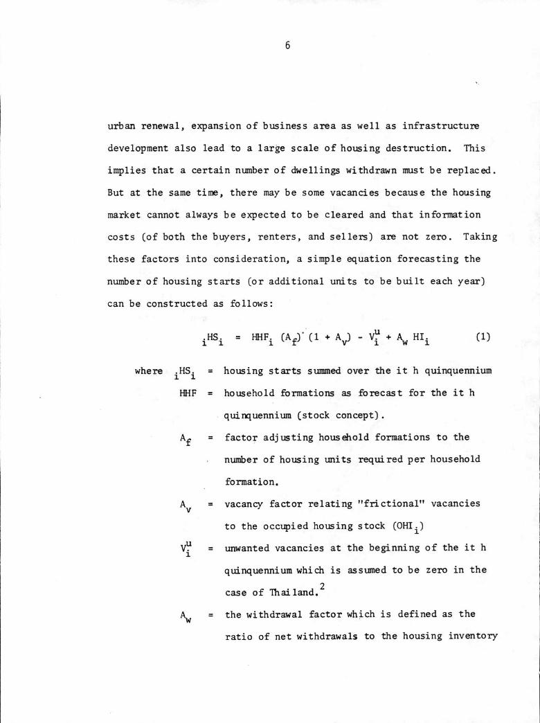
urban renewal, expansion of business area as well as infrastructure

development also lead to a large scale of housing destruction. This

implies that a certain number of dwellings withdrawn must be replaced.

But at the same time, there may be some vacancies because the housing

market cannot always be expected to be cleared and that information

costs (of both the buyers, renters, and sellers) are not zero. Taking

these factors into consideration, a simple equation forecasting the

number of housing starts (or additional units to be built each year)

can be constructed as follows:

where HS = housing starts summed over the i t h quinquennium

HHF = household formations as forecast for the i t h

quinquennium (stock concept) .

A£ = factor adjusting household formations to the

number of housing units required per household

formation.

A v = vacancy factor relating "fractional" vacancies

to the occupied housing stock (OHI.)

.HS. = HHF. (Af)* (1 + A y) - V 1

+ Aw HI. C D

unwanted vacancies at the beginning of the i t h

quinquennium which is assumed to be zero in the 2

case of Thailand. the withdrawal factor which is defined as the

ratio of net withdrawals to the housing inventory

7

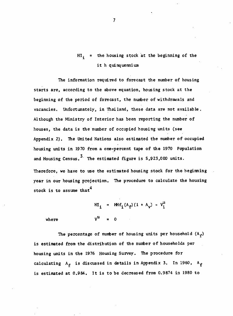
HI^ = the housing stock at the beginning of the

i t h quinquennium

The information required to forecast the number of housing

starts are, according to the above equation, housing stock at the

beginning of the period of forecast, the number of withdrawals and

vacancies. Unfortunately, i n Thailand, these data are not available.

Although the Ministry of Interior has been reporting the number of

houses, the data i s the number of occupied housing units (see

Appendix 2). The United Nations also estimated the number of occupied

housing units i n 1970 from a one-percent tape of the 1970 Population

and Housing Census.^ The estimated figure i s 5,923,000 units.

Therefore, we have to use the estimated housing stock for the beginning

year in OUT housing projection. The procedure to calculate the housing 4

stock is to assume that

HI i = HHf. (A f ) ( l + A v) - V?

where V u = 0

The percentage of number of housing units per household (A^)

i s estimated from the distribution of the number of households per

housing units i n the 1976 Housing Survey. The procedure for

calculating A f i s discussed i n details i n Appendix 3. In 1960, A f

is estimated at 0.984. I t i s to be decreased from 0.9874 in 1980 to

8

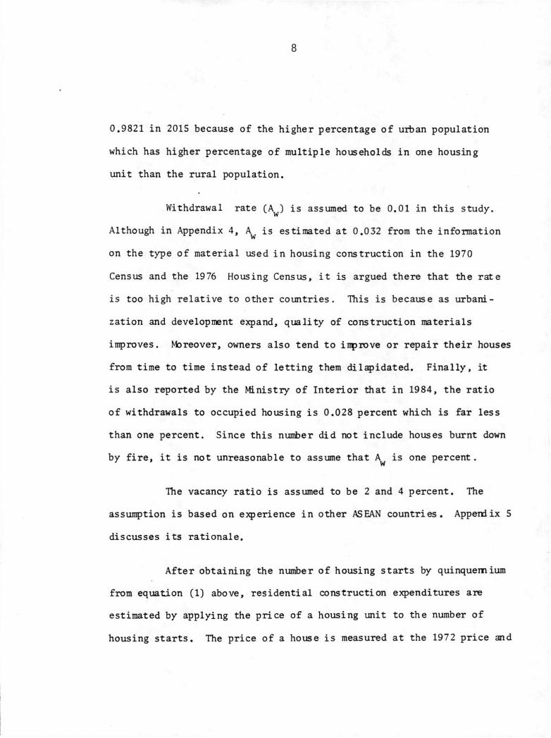
0.9821 in 2015 because of the higher percentage of urban population

which has higher percentage of multiple households in one housing

unit than the rural population.

Withdrawal rate (A ) is assumed to be 0.01 in this study. w

Although in Appendix 4, Aw is estimated at 0.032 from the information

on the type of material used in housing construction in the 1970

Census and the 1976 Housing Census, i t is argued there that the rate

is too high relative to other countries. This is because as urbani­

zation and development expand, quality of construction materials

improves. Moreover, owners also tend to improve or repair their houses

from time to time instead of letting them dilapidated. Finally, it

is also reported by the Ministry of Interior that in 1984, the ratio

of withdrawals to occupied housing is 0.028 percent which is far less

than one percent. Since this number did not include houses burnt down

by f ire , it is not unreasonable to assume that A^ is one percent.

The vacancy ratio is assumed to be 2 and 4 percent. The

assumption is based on experience in other ASEAN countries. Appendix 5

discusses its rationale.

After obtaining the number of housing starts by quinquennium

from equation (1) above, residential construction expenditures are

estimated by applying the price of a housing unit to the number of

housing starts. The price of a house is measured at the 1972 price and

9

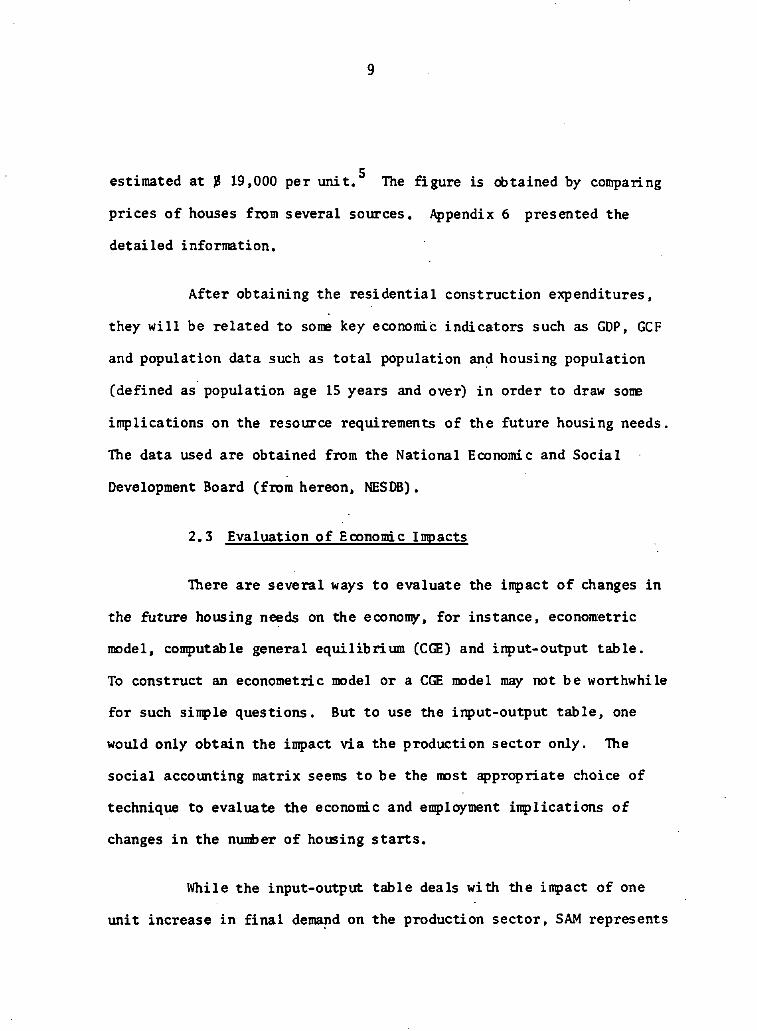
estimated at JJ 19,000 per unit. The figure is obtained by comparing

prices of houses from several sources. Appendix 6 presented the

detailed information.

After obtaining the residential construction expenditures,

they w i l l be related to some key economic indicators such as GDP, GCF

and population data such as total population and housing population

(defined as population age 15 years and over) i n order to draw some

implications on the resource requirements of the future housing needs.

The data used are obtained from the National Economic and Social

Development Board (from hereon, NESDB).

2.3 Evaluation of Economic Impacts

There are several ways to evaluate the impact of changes in

the future housing needs on the economy, for instance, econometric

model, computable general equilibrium (CGE) and input-output table.

To construct an econometric model or a CGE model may not be worthwhile

for such simple questions. But to use the input-output table, one

would only obtain the impact via the production sector only. The

social accounting matrix seems to be the most appropriate choice of

technique to evaluate the economic and employment implications of

changes i n the number of housing starts.

While the input-output table deals with the impact of one

unit increase in f i n a l demand on the production sector, SAM represents

10

the relationships between output, factor demands and income and the

decomposition of these relationship into separate effects . When

there i s an increase of one unit i n the f i n a l demand, production w i l l

increase, which i n turn, w i l l induce higher level of employment of

factors of production. Factor income, hence> w i l l increase. These

income w i l l be allocated to various institutions in the economy, i . e .

household, private corporation and government. They w i l l increase

their consumption (by the product of marginal propensity to consume

and the increase in income). This w i l l again stimulate an increase in

f i n a l demand which w i l l further induce more production i n the second

round. This effect i s called "intergroup effect 1 1 . Moreover, there

w i l l be a th i rd effect called extra-group ef fec t . This is . because

part of the income saved w i l l be reinvested which constitute another

source of f i n a l demand stimulation. These three effects are shown in

diagram 1 below.

Diagram 1

Impact of a Change i n Final Demand

Productions^

^ 1 N ^

^ Consumption 2

Investment

11

The social accounting matrix used i n this study is f i r s t

constructed to explore the employment implications of government

pol icy. (See Amaranand, et a l . 1984) The data base is 1981. It i s

consisting of 57 accounts. But since i t does not have a construction

sector i n the act ivi ty and commodity accounts, we have modified "SAW

to include the construction sector so that the impact of changes in

the construction sector can be evaluated.

Detailed description of SAM is provided in Appendix 10.

Table A-10 presents the 61 x 61 social accounting matrix i n 1981 and

Table A-11 gives the aggregated version of SAM 81. This report

employs the f ixed price multiplier , which i s also explained in

Appendix 7, to assess the economic impacts of a change in the f i n a l

demand for residential construction upon output of various sectors,

labor income, non-labor income, import mult ipl ier , forward and back­

ward linkages. A l l formulas are given i n Appendix 10.

3. Projection Results

In this section projection of number of households, housing

stock or inventory (HI), required housing additions (RA), and housing

starts (HS) based on equation 1 in part 2 are presented and discussed.

Estimates of real residential construction expenditures relative to

GDP and GCF (gross capital formation) w i l l also be given.

12

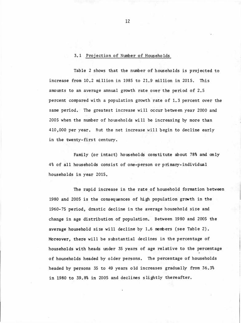
3.1 Projection of Number of Households

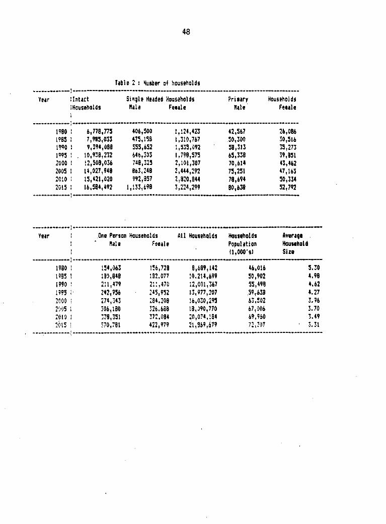
Table 2 shows that the number of households is projected to

increase from 10.2 million in 1985 to 21.9 million in 2015. This

amounts to an average annual growth rate over the period of 2.5

percent compared with a population growth rate of 1.3 percent over the

same period. The greatest increase will occur between year 2000 and

2005 when the number of households will be increasing by more than

410,000 per year. But the net increase wil l begin to decline early

in the twenty-first century.

Family (or intact) households constitute about 78% and only

4% of a l l households consist of one-person or primary-individual

households in year 2015.

The rapid increase in the rate of household formation between

1980 and 2005 is the consequences of high population growth in the

1960-75 period, drastic decline in the average household size and

change in age distribution of population. Between 1980 and 2005 the

average household size will decline by 1.6 members (see Table 2).

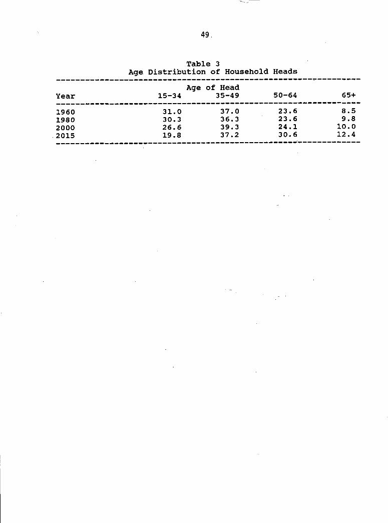
Moreover, there will be substantial declines in the percentage of

households with heads under 35 years of age relative to the percentage

of households headed by older persons. The percentage of households

headed by persons 35 to 49 years old increases gradually from 36.3%

in 1980 to 39.8% in 2005 and declines slightly thereafter.

13

The percentage of households headed by persons 49 years and over

remains relat ively stable unt i l the turn of the century and then

increases quite markedly (see Table 3).

3.2 .Housing Projection

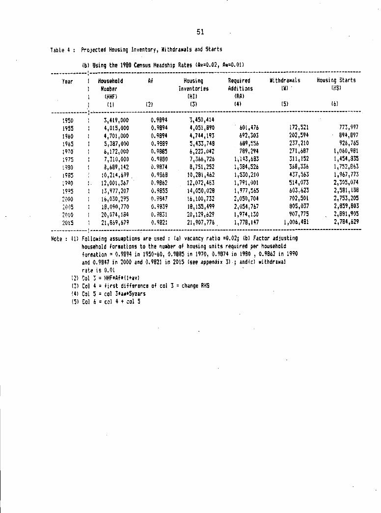
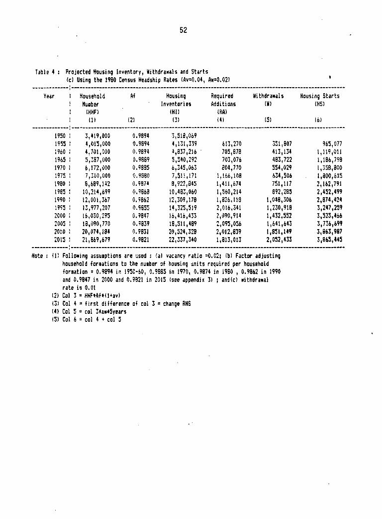
Table 4 gives quinquennial estimates from 1950 to 2015 of

the required housing stock, required additions, withdrawals and

housing starts based on equation (1). Three sets of predictions are

given. The f i r s t set is based upon the headship rate from the 1970

Census, and the second one on the headship rate from the 1980 Census.

Both sets assume that A y = 0.02 and ^ = 0.01. The third set i s also

based on the 1980 headship rate but with different assumptions of A y

and A w which are twice as high as the f i r s t two sets of predictions.

It should be observed that the results from the 1970 and 1980 headship

rates are not s ignif icant ly different , except that the 1970 headship

rates predict more number of households and required housing stock

unt i l year 2005, From thereon, the 1980 headship rate predict more

number of housing stock. The second observation from Table 4 and

estimates based on different assumptions about A y and A w (which are

not shown here) reveal that the required housing inventory (HI) and

required additions (RA) are not sensitive to different values of

vacancy rat ios, while the number of housing starts is quite sensitive

to the withdrawal rates. We, therefore, present the estimates of

housing inventory and housing starts based upon the assumption that

14.

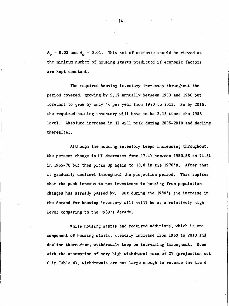
A y = 0.02 and A w = 0.01. This set of estimate should be viewed as

the minimum number of housing starts predicted i f economic factors

are kept constant.

The required housing inventory increases throughout the

period covered, growing by 5.1% annually between 1950 and 1980 but

forecast to grow by only 4% per year from 1980 to 2015. So by 2015,

the required housing inventory w i l l have to be 2.13 times the 1985

level . Absolute increase in HI w i l l peak during 2005-2010 and decline

thereafter.

Although the housing inventory keeps increasing throughout,

the percent change in HI decreases from 17.4% between 1950-55 to 14.5%

in 1965-70 but then picks up again to 18.8 in the 1970 ,s. After that

i t gradually declines throughout the projection period. This implies

that the peak impetus to net investment i n housing from population

changes has already passed by. But during the 1980's the increase in

the demand for housing inventory w i l l s t i l l be at a relat ively high

level comparing to the 1950's decade.

While housing starts and required additions, which i s one

component of housing starts, steadily increase from 1950 to 2010 and

decline thereafter, withdrawals keep on increasing throughout. Even

with the assumption of very high withdrawal rate of 2% (projection set

C in Table 4), withdrawals are not large enough to reverse the trend

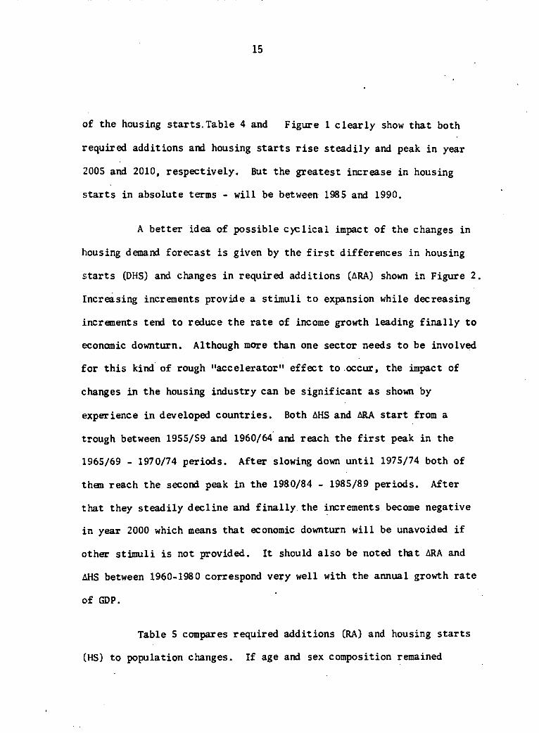
15

of the housing starts.Table 4 and Figure 1 clear ly show that both

required additions and housing starts r i se steadily and peak in year

2005 and 2010, respectively. But the greatest increase in housing

starts in absolute terms - w i l l be between 1985 and 1990.

A better idea of possible cyc l i ca l impact of the changes in

housing demand forecast is given by the f i r s t differences in housing

starts (DHS) and changes in required additions (ARA) shown in Figure 2.

Increasing increments provide a stimuli to expansion while decreasing

increments tend to reduce the rate of income growth leading f i n a l l y to

economic downturn. Although more than one sector needs to be involved

for this kind of rough "accelerator1 1 effect to occur, the impact of

changes in the housing industry can be significant as shown by

experience in developed countries. Both AHS and ARA start from a

trough between 1955/59 and 1960/64 and reach the f i r s t peak in the

1965/69 - 1970/74 periods. After slowing down un t i l 1975/74 both of

them reach the second peak in the 1980/84 - 1985/89 periods. After

that they steadily decline and f i n a l l y the increments become negative

in year 2000 which means that economic downturn w i l l be unavoided i f

other stimuli is not provided. It should also be noted that ARA and

AHS between 1960-1980 correspond very well with the annual growth rate

of GDP.

Table 5 compares required additions (RA) and housing starts

(HS) to population changes. If age and sex composition remained

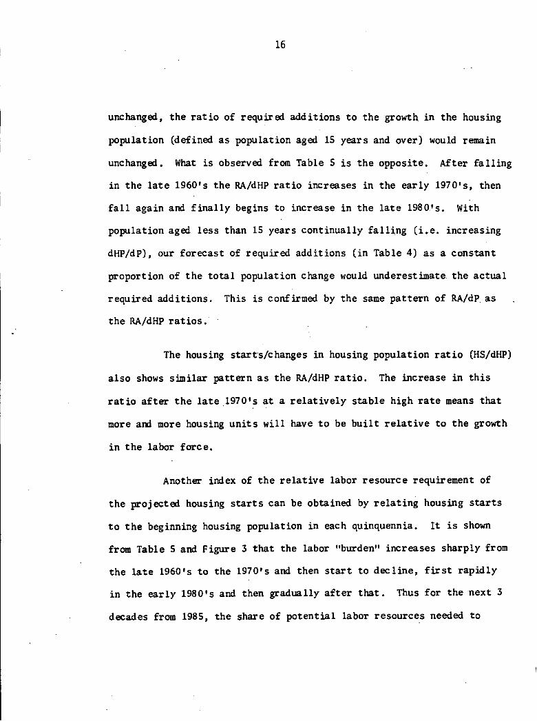
16

unchanged, the ra t io of required additions to the growth in the housing

population (defined as population aged 15 years and over) would remain

unchanged. What is observed from Table 5 is the opposite. After f a l l i n g

in the late 1960 ,s the RA/dHP rat io increases in the early 1970*3, then

f a l l again and f i n a l l y begins to increase in the late 1980's. With

population aged less than 15 years continually f a l l i n g ( i . e . increasing

dHP/dP), our forecast of required additions (in Table 4) as a constant

proportion of the total population change would underestimate the actual

required additions. This is confirmed by the same pattern of RA/dP. as

the RA/dHP ra t ios .

The housing starts/changes in housing population ra t io (HS/dHP)

also shows similar pattern as the RA/dHP ra t io . The increase in this

ra t io after the late 1970»s at a re la t ive ly stable high rate means that

more and more housing units w i l l have to be bui l t re la t ive to the growth

in the labor force.

Another index of the relat ive labor resource requirement of

the projected housing starts can be obtained by relating housing starts

to the beginning housing population in each quinquennia. It i s shown

from Table 5 and Figure 3 that the labor "burden11 increases sharply from

the late 1960's to the 1970's and then start to decline, f i r s t rapidly

in the early 1980fs and then gradually after that. Thus for the next 3

decades from 1985, the share of potential labor resources needed to

17

supply new housing required by population changes and withdrawals at

a constant rate w i l l be declining steadily.

A l l the evidence presented so far show that the rapid decline

in population projection from 1980-2015 w i l l have much effects in

lessening the demand for housing in the next 3-4 decades.

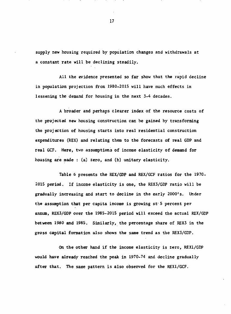
A broader and perhaps clearer index of the resource costs of

the projected new housing construction can be gained by transforming

the projection of housing starts into real residential construction

expenditures (REX) and relating them to the forecasts of real GDP and

real GCF. Here, two assumptions of income e las t ic i ty of demand for

housing are made : (a) zero, and (b) unitary e las t i c i ty .

Table 6 presents the REX/GDP and REX/GCF ratios for the 1970-

2015 period. If income e las t ic i ty i s one, the REX3/GDP rat io w i l l be

gradually increasing and start to decline in the early 2000's. Under

the assumption that per capita income i s growing at* 5 percent per

annum, REX3/GDP over the 1985-2015 period w i l l exceed the actual REX/GDP

between 1980 and 1985. Similarly, the percentage share of REX3 in the

gross capital formation also shows the same trend as the REX3/GDP.

On the other hand i f the income e las t ic i ty i s zero, REX1/GDP

would have already reached the peak in 1970-74 and decline gradually

after that. The same pattern i s also observed for the REX1/GCF.

18

These findings imply that, residential construction can s t i l l play

a v i t a l role in accelerating the nation's economic growth i f income

growth at a high enough rate. Had income fa i l ed to increase,

residential construction w i l l no longer be a key factor in accelerating

growth because slower population growth w i l l begin to reduce the .

demand for housing starts over the projection period.

If the f i r s t differences of REC i s calculated just l ike the

f i r s t differences of housing start (AHS), more information about

possible cyc l i ca l impact of changes in housing expenditure can be

obtained. Figure 4 depicts REX under various assumption of E . and g.

If Ey is zero, A REX1 shows similar declining pattern as AHS in

Figure 2 after the 1980-85 to 1985-90 period. But i f the assumption

of positive E^ is used, then residential construction expenditure w i l l

s t i l l provide an strong stimuli to expance the economy income. I f per

capita GDP is 5% per year then we would expect the construction sector

to be growing at a steep rate between the period of 1975-80 to 2010-

2014. But i f g i s 4%, then there may be a slowdown of REX in year

2000-04 and 2005-2009.

3,3 Housing Quality, Income Growth and Demographic Factors

We have found that although the number of housing starts and

housing inventory w i l l be increasing throughout the projection period,

the decreasing increments of housing starts (AHS) w i l l lead to

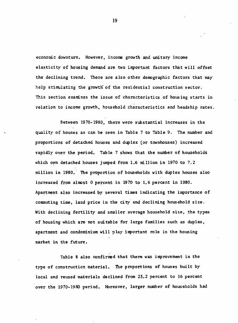
19

economic downturn. However, income growth and unitary income

e las t ic i ty of housing demand are two important factors that w i l l offset

the declining trend. There are also other demographic factors that may

help stimulating the growth' of the residential construction sector.

This section examines the issue of characteristics of housing starts in

relation to income growth, household characteristics and headship rates.

Between 1970-1980, there were substantial increases in the

quality of houses as can be seen in Table 7 to Table 9. The number and

proportions of detached houses and duplex Cor townhouses) increased

rapidly over the period. Table 7 shows that the number of households

which own detached houses jumped from 1.6 mil l ion i n 1970 to 7.2

mil l ion i n 1980. The proportion of households with duplex houses also

increased from almost 0 percent in 1970 to 1.6 percent i n 1980.

Apartment also increased by several times indicating the importance of

commuting time, land price in the ci ty and declining household s ize .

With declining f e r t i l i t y and smaller average household size, the types

of housing which are not suitable for large families such as duplex,

apartment and condominium w i l l play important role in the housing

market in the future.

Table 8 also confirmed that there was improvement in the

type of construction material. The proportions of houses buil t by

local and reused materials declined from 23.2 percent to 16 percent

over the 1970-1980 period. Moreover, larger number of households had

20

water supply, e lectr ic l ight ing, and better to i le t f a c i l i t y as shown

in Table 9.

These improvements i n the quality of housing coincided with

the rapid increase of real GDP during the 1970's. It also implies that

the income e las t ic i ty of housing demand is high and that our assumption

of unitary income e las t ic i ty which is based on the estimate by Mason

(1987) i s r e a l i s t i c . Therefore, our base projection (zero income

elas t ic i ty) that residential construction w i l l decline may not happen

i f we allow for income growth in the future. Housing starts i n the

next few decades w i l l be of better quality which means higher con­

struction expenditure. The second factor that may have positive effect

on the residential construction is that household with heads 35 to 49

years of age w i l l grow most rapidly while households with younger heads

w i l l grow most slowly (see Table 3). Almost 69 percent of heads w i l l

be i n the 35-64 age groups in 2015 comparing with 60 percent i n 1980.

These household heads w i l l certainly have higher average income than

both the younger and the older heads. Therefore, quality of housing

starts can be expected to be greatly improved in the next 3 decades.

Thirdly, although the headship rates in 2015 are projected to be lower

than those in 1980 (see Figure A - l i n Appendix 1), the ratio of

population aged 15-29 w i l l increase as a result of f e r t i l i t y decline.

The declining ratio may have the positive effect on the relative

income of the two groups of population (Campbell, 1982). Increasing

21

relat ive income of population aged 30-64 w i l l , in turn, increase the

headship rates which implies more housing starts .

Another demographic factor that may affect the quality of

housing is the average household size and the average age of household

members. As can be seen in Figure 5, the average household size w i l l

drast ical ly decline in the next three decades. Smaller household size

means that fewer bed-rooms and smaller but higher quality houses can

be b u i l t . Since the average number of members under 15 years of age

w i l l decline drastically during the next two decades (see Mason, e t . a l . ,

1986, Table 19), family members w i l l become older. The characteristics

of housing starts demanded by those older members w i l l , therefore, be

affected.

3.4 Modelling Housing Characteristics

The demand for housing characteristics of the u t i l i t y -

maximizing u t i l i t y can be written as :

H = H (P, Y ,

where H i s the demand for housing characteristics

P is the relat ive price

Y i s the household income

i s the demand shifters such as demographic variables.

22

We w i l l use the above model to forecast the future housing

characteristics by making use of the projection of demographic

variables derived from HOME.

There are a large number of dimensions of housing

characteristics. In this study, we classify housing characteristics

into 5 categories, i . e . (a) type of l iv ing quarters, (b) number of

bedrooms, (c) type of construction materials, (d) type of t o i l e t ,

bathroom, and (e) exclusive use of to i l e t and kitchen. These

characteristics are the dependent variable i n our demand model. Table

10 shows that there are a total of 17 demand equations of housing

characteristics. The def ini t ion of the dependent variables i s also

given i n the some table.

The demand for housing characteristics are postulated to

depend upon age of head, sex of head, age composition of household

members, type of household, permanent income of the household and price

of the characteristics.

Since the data source that we w i l l employ does not contain

income and price information, we w i l l use some proxies for household

income. Besides education of the head which also represents taste of

the head, 'occupation of the head and avai lab i l i ty of certain assets

can be good measure of permanent income. We choose to use the

avai lab i l i ty of television and refrigerator as the proxy for assets.

23

The variable i s a dummy variable with a value of one i f the household

has a television set or a refrigerator, otherwise i t i s zero. The

l i s t of the independent variables are given i n Table 11.

Age of head and i t s squared are included to represent the

l i fe -cyc le pattern of demand for housing characteristics of people at

different age group. For example, when a head is very young, he may

not be able to afford or may not need a large house. As he grows

older, the need and abi l i ty also increases, but f i n a l l y decrease at

some later age*

Number of household members at each age is posit ively

affecting the demand for bedrooms, and type of l i v ing quaters. A

family with small children may not need ah extra bedroom, but not a

family with older children. Moreover, the former can easily l ive in

apartment or row house while the lat ter may have to f ind a detached

house, other things being equal.

Type of household w i l l also affect the choice of l i v ing

quarter. For example, a one-person or a single head household w i l l

have more tendency to l ive i n a room-house or a row house. But at the

same time, they may be able to afford exclusive bathroom and flush

t o i l e t .

Sex of the household head is included to control for male-

female differences in taste for housing characteristics. The variable

is a dummy variable.

24

. Education of head is measured by four dummy variables, i . e . ,

no education, primary, secondary and tertiary education. A head with

no education is the reference variable omitted from the equation. We

expect the head with tertiary education to demand higher quality of

house than those with lower education.

Occupation of head i s also the proxy for income. There are

f ive groups of occupation : (a) professional workers, (b) managerial

workers, (c) other white collar workers, (d) blue collar workers and

(e) other workers which are the reference.

Moreover, four employment status variables are also included

to be proxy for income. They are employers, government employees,

private employees, and the reference group which consists of se l f -

employed persons and unpaid family workers.

Persons who l ive i n the urban area tend to l ive i n a smaller

house such as apartment, row house and roomhouse because of high price

of land. But the smaller house i s usually compensated by high quality

type of housing, e.g. , exclusive and fluch t o i l e t , cement house, etc.

Since the dependent variables under item number 1, 3 and 4

in Table 10 are dichotomous, the appropriate functional form should

be logit or probit function. But there are about 67,392 households in

our data set obtained from the Thai census, estimation of logi t or

probit w i l l be extremely expensive. We, therefore, decide to employ

25

ordinary least squares technique which w i l l give us biased estimates

of c o e f f i c i e n t s . But i t i s worth to pay the cost of biasness for two

reasons. F i r s t , we have very limited computer budget. Secondly, our

main objective i s only .to provide a framework to forecast housing

characteristics for the planner.

The demand for number of bedrooms and number of other rooms

used f o r sleeping (item number 2 i n Table 10) w i l l be estimated by

OLS technique.

A single equation approach w i l l be used to estimate the

demand for housing c h a r a c t e r i s t i c s . I t i s wellknown that the sin g l e

equation estimate of demand function w i l l give us biased results due

to simultaneity problem. Moreover, there i s also l i m i t a t i o n arises

from the omission of the price variables. However, studies of the

simultaneity problem and review of l i t e r a t u r e found that estimated

income e l a s t i c i t i e s and effects of demographic variables are i n l i n e

with single equation estimates (S. Malpezzi and S.K. Mayo 1987,

p. 703-705) .

Our data source i s the one-percent sample tape of the 1980

Population and Housing Census of Thailand. The data set consists of

67,392 households a f t e r dropping cases with unknown observations.

26

3.5 Regression Results of Housing Characteristics

Although we have estimated IS regressions of housing

characteristics and the results are provided i n Appendix 10, we w i l l

only use 11 equations (those with asterisk i n Table 10) to forecast

the future characteristics of houses. Table 12 presents the means and

S.D. of a l l variables* We w i l l only discuss the interes t i n g r e s u l t s .

Among the regressions of type of l i v i n g quarters, detached

house and row house equations have highest adjusted R-square, i . e . ,

0.28 and 0*23, respectively. Other equations have very small R-square.

So i n our projection, we w i l l use only the detached house and the row

house equations to do a forecast.

In the detached house regression, only one variable i s not

s i g n i f i c a n t , i . e . HDEDSEC. Most variables have expected sign. As a

family head grows older, the probability of having a detached house i s

also higher. But a f t e r the age of 64 years, the pr o b a b i l i t y declines.

Male head has lower p r o b a b i l i t y of having a detached house than female

head. Head with a l l levels of education, except secondary l e v e l , have

higher tendency to have a detached house than one with no education.

However, well-to-do household (TVREF) or household with a head who i s

employer w i l l have lower pro b a b i l i t y of having a detached house.

Farmers w i l l have higher tendency to have a detached house than people

i n other occupations. This i s also true of a household i n the r u r a l

area vis-a-vis urban area, female head v i s - a - v i s male head.

27

As the family head grows older, he (or she) w i l l have lower

prob a b i l i t y of having a row house. After the age of 64, the s i t u a t i o n

i s reversed. Households which have higher pr o b a b i l i t y of l i v i n g in

the row house have the following characteristics : (a) head has no

education ; (b) head i s a self-employed worker or an employer ; (c)

head i s a farmer ; (d) head i s male ; and (e) they l i v e i n the urban

area.

Among the regressions of type of construction materials,

only the cement regression has a good f i t with R-square of 0.23.

Younger household head has higher p r o b a b i l i t y of having a cement house.

The cha r a c t e r i s t i c s of the household whose house i s made of cement

are as follows: (a) head has at least secondary education; (b) he i s

an employer and his occupation i s professional, management or white

c o l l a r job, (c) the household has t e l e v i s i o n and r e f r i g e r a t o r and

l i v e s i n the urban area; (d) the higher the number of family members

aged 15 years and over, the higher the pro b a b i l i t y of having a concrete

house.

In the wood regression, the function has an inverted U-shape

with respect to. age of head. I f a head has college education, an

employer, a private employee, a manager or white c o l l a r worker, he w i l l

have higher tendency to l i v e i n a wooden house. Rich household (as

measured by TVREF) and household i n the urban area have lower

pr o b a b i l i t y of having a wooden house.

28

The bedroom equation has probably the most meaningful r e s u l t .

The c o e f f i c i e n t of age i s positive and that of age squared i s negative

as expected. Household head with higher income as measured by

education, and occupation tend to have more bedrooms. Government

and private employees have smaller number of bedrooms than s e l f -

employed heads, but employer has more bedrooms. As the number of

family members increases, more bedrooms are required. But the effect

i s not linear with respect to age of family members. Adult member

demand more rooms than younger member. For example, an increase of

one member aged 0-5 years w i l l demand 0.24 more rooms, but an equal

increase of the member aged 30 years and over w i l l demand about 0.2

more rooms. The difference i s f i v e times. Urban and r i c h household

tend to have more bedrooms than r u r a l and poor household.

The households with higher p r o b a b i l i t y of having exclusive

bathrooms and kitchen are : (a) urban household, (b) t h e i r hea has

high education; (c) he i s not a famer; (d) the household has TV or

re f r i g e r a t o r . Female head also tend to have exclusive bathroom more

than male head. Both one-person household and single head household

have higher p r o b a b i l i t y of having exclusive bathroom than other

family type. But only single head household has more change of having

exclusive kitchen than others. Male and female heads are not d i f f e r e n t

with regards to exclusive use of kitchen.

29

While younger household had have higher p r o b a b i l i t y of

having f l u s h t o i l e t , the older head tend to use l a t r i n e t o i l e t . This

i s probably the influence of western culture among younger population.

Head with college education has lower probability of using l a t r i n e

t o i l e t probably because they l i k e to use flush t o i l e t since the

co e f f i c i e n t of HDEDCOL i n the flush equation i s positive and s i g n i f i c a n t .

Uneducated head and r u r a l household tend not to use both flush and

l a t r i n e t o i l e t . While private employee l i k e s to use flush and d i s l i k e s

l a t r i n e t o i l e t , government employee's taste i s the other way round.

3.6 Forecast of Housing Characteristics

Table 13 i s a summary of the forcast of 5 type of housing

ch a r a c t e r i s t i c s . Detailed forecasts which are also done for various

type of households are given i n Appendix 11.

To forecast future housing c h a r a c t e r i s t i c s , we employ 11

regressions (those with asterisk i n Table 11) shown in Appendix 10.

The projection of the independent variables which are demographic

and educational variables are obtained from HOMES. Other independent

variables are assumed to be constant at their mean values over the

entire projection period. The sum of the product of the regression

co e f f i c i e n t s and the projected values of independent variables give

us the future housing characteristics reported i n Table 13.

30

The percentage of detached house and other type of houses

are projected to increase marginally by one percent each over the

1980-2015 period. Percentage share of row houses w i l l decline by

2 percent over the same period. These results imply that changes i n

demographic variables w i l l have only marginal effect on the housing

char a c t e r i s t i c s . Changes i n economic factors such as income (as

measured by TVREF) and occupation w i l l be the important determinants

of housing characteristics because the magnitude of these c o e f f i c i e n t s

i s the largest.

There i s also no s i g n i f i c a n t change i n the type of

construction materials and the number of bedrooms or rooms used for

sleeping purpose over the 1980-2015 period i f only demographic

variables are allowed to change. Again construction materials used

w i l l be l a r g e l y affected by changes i n income, occupational structure

and employment status because of the r e l a t i v e l y large s i z e of t h e i r

c o e f f i c i e n t s . >

However, the projected r e s u l t s show that there are s i g n i ­

f i c a n t changes in the use of bathroom and type of t o i l e t . Over the

projection period, exclusive use of bathroom jumped from 29 percent

to 35 percent while shared use of bathroom declined to 65 percent.

Between 1980 to 2015, the percentage share of flu s h t o i l e t

and l a t r i n e t o i l e t w i l l increase by 3 percent and 6 percent,

31

respectively. The other type of bathrooms w i l l decline by 10 percent

over the same period.

We can conclude that, f i r s t , the demographic variables have

sig n i f i c a n t effects on the exclusive use of bathroom and type of

t o i l e t , but not on other type of housing characteristics. Secondly,

i t seems that changes i n economic factors w i l l have more influence

upon the demand for housing c h a r a c t e r i s t i c s . Thirdly, since our

projection s t i l l ignore price variable, i t i s possible that changes

i n prices, such as increase i n price of wood w i l l have s i g n i f i c a n t

effect on the type of construction materials and type of housing

characteristics demanded i n the future.

4. The Construction Sector

Before discussing the impacts of construction expenditures

on the economy, a b r i e f discussion of the construction sector w i l l be

presented.

4.1 Overview of the Construction Sector

The construction sector i s the s i x t h largest economic sector

i n term of GDP. In 1984, i t s GDP share was 5.3 percent comparing to

6.1 percent i n 1970. According to the Labor Force Survey, t h i s sector

exmploys approximately 0.53 m i l l i o n workers or about 2.5 percent of

32

t o t a l employment i n 1984. The employment share i s surprisingly low

comparing to the GDP share of the construction sector. This i s

p a r t l y because a large number of construction workers go back to t h e i r

farming a c t i v i t y i n the wet season. In the dry season (January-March),

employment i n the construction sector increased by 0.22 m i l l i o n

persons, while t o t a l employment shrinked by 3.7 m i l l i o n . So employment

share of the construction sector i s 3.4 percent. Moreover, a large

number of farmers are also part time workers i n the construction

sector. Most of them learn the construction s k i l l from t h e i r parents

and t h e i r own experience.

Investment i n the construction sector as measured by gross

c a p i t a l formation (GCF) was 95,800 m i l l i o n baht or 47 percent of GCF

i n 1984. ' About 50% of the construction investment i s public investment.

This i s a normal phenomena f o r a developing country l i k e Thailand where

the government assigns high p r i o r i t y to i t s development projects.

Within the construction sector, r e s i d e n t i a l construction i s

the largest subsector. In 1984, t o t a l r e s i d e n t i a l construction

expenditure was 31 m i l l i o n baht or 32 percent of t o t a l construction

expenditures. The percentage share of r e s i d e n t i a l construction

expenditure has been fluctuating from the highest level of 42% i n 1961

to the lowest l e v e l of 20.5 percent i n 1979. Fluctuations i n con­

struction expenditure and gross c a p i t a l formation can be explained by

the growth rates of GDP shown i n Appendix 8. For example, the decline

33

i n the construction expenditures i n 1979 and 1982 coincided with the

decreases i n the growth rate of GDP from 9% i n 1977 to 5.8% i n 1979

and from 6.1% i n 1981 to 4.1% i n 1982.

Residential construction also varies d i r e c t l y with economic

growth as can be seen from data i n Appendix 8. Moreover, during 1984-

1986 when the long-term nominal lending interest rate was at the

highest level of 16% - 17%, r e s i d e n t i a l construction p a r t i c u l a r l y

investment by the real estate companies was stagnant. Since late

1986, interest rate has come down.to the l e v e l of 12% to 13%,

r e s i d e n t i a l construction has picked up rapidly. As a consequence,

prices of construction materials have gone up.

Unlike Indonesia and Korea, Thailand has not experienced

severe housing shortages. Although the economy has been growing at

the very high rate since 1960, i t was not u n t i l early 1970's when the

private housing market started to expand. This i s probably caused by

the high value of income e l a s t i c i t y of demand for housing. The growth

of the supply of housing was not impeded by any government regulations

because the government i s always too slow to l e g i s l a t e laws and

regulations. The rapid increase i n the number of condominium i n the

early 1980fs also caused public concern because they are not subject

to special regulations, especially f i r e control.

Although there are not many large real estate companies,

there are a large number of small companies i n the housing market.

34

Prices are very competitive and always r e f l e c t the q u a l i t y of the

houses sold. Small company can e a s i l y get loan from the commercial

bank and develop a small piece of land on which 50-100 town-houses can

be b u i l t . The prices of one unit of a two-storey townhouse on a 6 x

10 meters plot of land can vary from B 150,000 to 1,000,000 depending

upon the location and q u a l i t y .

Most of the houses i n Bangkok b u i l t by the real estaste

companies are i n the suburb areas especially i n the eastern part and

along the highway to the North where the government provides r e l a t i v e l y

better public u t i l i t i e s and s o c i a l i nfrastructure.

There are two other factors that make i t possible for the

rapid growth of the housing market. The f i r s t factor i s the rapid

population growth i n the 1960-1975 period. Bangkok has probably

experienced the highest rate of growth due to rural-urban migration.

The second factor i s that Thailand did not have the problems of

shortages of construction workers and construction materials,

especially wood and cement. Although there were temporary shortage of

cement i n the late 1970's due to p r i c e control, Thailand has now

become an exporter of cement a f t e r the p r i c e control was l i f t e d i n

1979, Even though there are a few large suppliers of construction

materials, especially the Siam Cement group, competition from small

l o c a l producers i s very strong. Such competition helps keep down the

cost and price of houses.

35

The housing sector has also benefited from the abundant

supply of forest. In the recent years, prices of wood products have

been increasing rapidly i n response to increasing shortages. However,

wood products are s t i l l major construction materials i n Thailand.

The above discussion does not mean that Thailand does not

have housing problems. One of the important problems i n the housing

market i s finance. Table 14 shows the d i s t r i b u t i o n of loan made by

the commercial banks and the finance companies. Their major business

i s i n the sectors of manufacturing and trade. Housing mortgage loan

represents only 3.2% of commercial bank loan and only 2.8% of the

finance company loan. Since the interest rates charged to different

loan types are s l i g h t l y d i f f e r e n t , and returns to loan for manufacturing

and trade are r e l a t i v e l y higher, commercial banks are not very keen at

expanding housing loan. Although more than 50% of housing loan, or

$ 17 m i l l i o n i n 1985 (see Table 14), i s provided by the commercial banks,

only a few banks are serious i n providing housing loan to t h e i r

customers•

I t i s also apparent that most finance companies are not

interested i n providing mortgage loan. Less than 3% of t h e i r loan i s

for mortgage because rate of return to housing loan i s lower than other

sectors. And yet they provide as high as 11% of loan to the real

estate development projects.

36

According to Table 15, the second largest supplier of

housing credit i s the Government Housing Bank. However, i t s credit

expansion i s severely limited by the regulations of the Finance

Ministry and bureacratic procedures.

Credit fonciers and the NiA which should play active role

i n housing mortgage are not important actors i n the housing market.

Most of the loan of the credit fonciers i s for other a c t i v i t i e s which

are more p r o f i t a b l e than housing loan. Due to regulations on

promissory notes the credi t fonciers' cost of ca p i t a l i s 2% - 3%

higher than that of the commercial banks. This forces them to

provide loans to the sectors that they can charge higher interest rate

Cbased on a f l a t rate basis where interest does not decline with the

amount of p r i n c i p a l owed), e.g. rental purchase. They cannot charge

the same high rate of interest for mortgage loan because the interest

cost w i l l be too high for the consumers.

There are two major constraints that l i m i t the role of the

fi n a n c i a l i n s t i t u t i o n s i n housing loan a c t i v i t i e s (Prasart Tangmatitham

1987). F i r s t , while credit fonciers (or b u i l d i n g societies or Savings

and Loan Association) i n developed countries can mobilize short term

c a p i t a l , those i n Thailand are required to raise t h e i r fund by issuing

long-term notes (at least one year maturity). As a r e s u l t , t h e i r

c a p i t a l cost i s higher than that of commercial banks because long-term

interest rate i s higher. But they have to charge the same competitive

37

loan rate for t h e i r mortgage loan. Secondly, the Government Housing

Bank's lending rate i s 1% - 2% lower than other f i n a n c i a l i n s t i t u t i o n .

This i s i n fact a subsidy for i t s customers. Moreover, depositors at

the GHB are exempted from tax on interest income. But those who

obtain mortgage loan from other i n s t i t u t i o n s are not subsidized.

Since the objective of the GHB i s to help the poor to secure mortgage

loan, the subsidy should be limited only to poor customers. Elimination

of interest subsidy except the low income customers w i l l allow the

finance companies and credit fonciers to expand t h e i r r o l e i n mortgage

loan.

In the urban area there are problems of poor and unsanitated

housing especially i n the slum areas which have been expanding as a

resu l t of urbanization and large number of in-nri.grants. This i s

probably one of the reason many rural migrants migrate only temporarily

to Bangkok. Although the National Housing Authority (NHA) has attempted i

to solve the problems by building low cost apartment for them, the

projects are not very successful. F i r s t , many slum dwellers cannot

afford the low cost apartment. Secondly, the NHA only b u i l d a small

number of houses i n each year. F i n a l l y , many people r e s e l l t h e i r

apartment either because they get good p r i c e or because t h e i r workplace

i s too far from t h e i r new house. Realizing the last problem, the NHA

has now begun to i n i t i a t e j o i n t projects with the large-scale private

companies or public agencies. The projects are to buy the land close

38

to the companies or government o f f i c e s and b u i l d the low-cost houses

and s e l l them to the employees of those agencies. So far, there have

been only a few of t h i s kind of projects.

In the r u r a l area, there seems to be no serious housing

problems i n term of the place to l i v e . But i t i s usually observed

that most of the r u r a l houses are of low quality. They are made of

reused materials, palm leaves and bamboo rods which have short l i v e .

Young couples usually b u i l d a bamboo hut i n t h e i r farm and w i l l begin

to b u i l d a new and stronger house once they have enough saving. In

every part of the country, farmers w i l l s t a r t b u i l d i n g or renovating

t h e i r houses i n the summer when they are free from farm a c t i v i t i e s .

This i s why most construction workers i n the c i t y come from the r u r a l

areas, especially from the Northeast and the North where wood i s

abundant and they have carpenter s k i l l . However, i t should be noted

that i n the l a s t few years there are a large number of new houses of

modem style which are b u i l t of high qu a l i t y material made i n the

c i t y . In the Northeast, i t i s the money earned from the Middle East

that enables the r u r a l inhabitants to enjoy luxurious houses. In

other regions, especially i n the Central P l a i n i t may be because of

the r i s i n g income of farm households due to the facts that Thai

farmers have rapidly d i v e r s i f y t h e i r produces i n such a way as to

benefit from the world market.

39

4.2 Impacts of Construction Expenditures

Appendix 10 presents the fixed price m u l t i p l i e r s (Ma)

obtained from equation (2). The exogeneous variables i n the equation

are government, t o u r i s t , rest of the world (export) and capital since

Thailand i s a small open economy.

Since the data do not allow us to obtain a separate account

for the r e s i d e n t i a l construction expenditure, the account of

construction w i l l be used to estimate the impacts of changes i n

r e s i d e n t i a l construction expenditures on the economy.

Table 16 presents part of the fixed p r i c e m u l t i p l i e r s

obtained from Appendix 10. The general conclusion drawn from the

table i s the r e l a t i v e constancy of mu l t i p l i e r s along rows of the table.

For example, an i n j e c t i o n of 100 baht into any a c t i v i t y results i n a

fixed price m u l t i p l i e r effect on the construction sector. The effect

i s i n a range of 5.96 to 1.02 baht. The implication i s that the

second- and third-order effects on the economy6 are largely independent

of the structure of demand. The homogeneity of higher-order effects

i s also important for the structure of employment and income d i s t r i ­

bution. Table 17 shows that whichever a c t i v i t y , except the government

sector, might be expanded, hired labor income multip l i e r s are i n the

range of 0.26 to 0.40.

40

An i n j e c t i o n into any a c t i v i t y w i l l produce the largest

effect on the income of those with primary education. The effects on

the income of people with more than primary education are r e l a t i v e l y

small no matter which a c t i v i t y i s expanded. The exception i s the

government sector which i s the largest employers of educated persons.

Comparing with other sectors, an i n j e c t i o n into the con­

struction section w i l l produce the second largest s i z e of m u l t i p l i e r

(2.69) as shown i n Table 16 . The m u l t i p l i e r on the i n d u s t r i a l sector

(1.33) i s the largest one. However, the expansion of the construction

sector w i l l also lead to a large increase i n import with a m u l t i p l i e r

of 0.4885 which i s only second to the import m u l t i p l i e r of the

expansion of the state enterprise (0.6794).

In term of forward linkages, the construction sector has

strong forward linkage e f f e c t on the i n d u s t r i a l (1.367), the

a g r i c u l t u r a l (1.0) and the service (0.965) sectors. I f we read along

the diagonal of the lower part of Table 10, i t can be seen that the

construction sector has the second largest forward linkages (9.08) on

i t s e l f a f t e r the government sector (12.68).

However, the results i n Table l i shows that the construction

sector has small backward linkages with other sectors. The values of

the linkages, except the linkage on i t s e l f (6.887), are between 0.47

and 0.61.

41

Table 1 7 shows that an i n j e c t i o n into the construction

sector w i l l produce the fourth largest m u l t i p l i e r on the income of

hired labor (0.3609) and own-account workers CO-3087), but w i l l have

the second largest m u l t i p l i e r (0.80) on the income of the c a p i t a l

owners. Expansion of the government sector w i l l have largest impact

on hired labor income (1.116), while the a g r i c u l t u r a l expansion w i l l

produce highest impact on the income of own-account workers. Income

of the c a p i t a l i s t s w i l l be increased by the largest size i f the

service sector i s stimulated.

Table 17 also allows us to consider the impact of con­

struction expansion on the income of various groups o f persons broken

down by educational l e v e l and occupation. The table shows that i f

the construction sector i s stimulated, persons who have only primary

education or lower w i l l have highest increase i n t h e i r income

regardless of the sources of income, ( i . e . wage income, own-account

workers 1 income or c a p i t a l income). The higher the education l e v e l ,

the lower the m u l t i p l i e r i s .

The expansion of the construction sector tends to increase

income of the blue c o l l a r workers (0C4) who are hired labor more than

other occupation groups. But for own-account workers, the income

effects on each occupation subgroups depend upon t h e i r educational

l e v e l s . For example, i f the persons have primary education, those

who are i n the service occupation (0C3) w i l l have highest income i n

42

t h e i r income. For college graduate, the highest m u l t i p l i e r s are i n

the professional and management (0C1) and clerks (0C2).

The construction expansion has the largest impact on the

income of corporations (0.32) and the second largest impact i s on the

c a p i t a l income of those in the non-agricultural sector (0.0428).

Farmers also share r e l a t i v e l y high benefit from the expansion of t h i s

sector with the m u l t i p l i e r of 0.0379.

5. Conclusion

This study employed a more refined method of headship rate

to forecast the number of households i n the year 1985-2015. The method

b a s i c a l l y c l a s s i f i e s families into 4 types : namely the intact

households, the households i n which the spouse i s not present, the

primary individual households, and the one-person households.

The results show that although housing inventory and housing

starts increase throughout the projection period, the growth rates of

housing inventory and housing starts during the projection period

w i l l be slower than those i n the 1950-1980 period. Though housing

st a r t s w i l l peak i n 2010, the greatest increases - i n absolute terms-

w i l l be between 1985 and 1990. These results are not surprising

since Thailand has already been experiencing a rapid decline i n

f e r t i l i t y since the mid 1970's. I f the forecast were correct and

other things remained the same, the decline i n the changes i n housing

43

s t a r t s would lead-to economic downturn. However, from the optimistic

viewpoint, the decreasing increments of housing s t a r t s could be

interpreted d i f f e r e n t l y , i . e . , r e l a t i v e l y less resources would be

needed i n order to provide the same le v e l of e x i s t i n g housing

standard to the future population. Hence more resources can be

diverted to other uses including better quality housing i n the future.

Different assumptions about income e l a s t i c i t y of housing

demand and income growth are also employed i n the projections.

Comparing with the base projection where income e l a s t i c i t y i s zero,

the results show that income growth and degree of income e l a s t i c i t y

w i l l be important factors stimulating the growth of the r e s i d e n t i a l

construction sector.

Data on housing q u a l i t y from two censuses — 1970 and 1980 —

reveal that there were substantial improvements i n housing q u a l i t y .

Since HOMES also projects smaller household s i z e , higher proportion

of households with heads aged 35-49 years, and larger proportion of

older family members, these demographic factors w i l l c e r t a i n l y affect

the type and q u a l i t y of housing starts that w i l l be demanded i n the

next 30 years.

The growth of the r e s i d e n t i a l construction sector i s

discussed i n the report. Factors contributing to and hindering

growth are i d e n t i f i e d . The favorable factors include the w e l l -

functioning of the private housing sector with minimal government

44

regulations and abundance of supply of construction materials as well

as s k i l l e d construction workers. Government regulations of the

finance companies and credit fonciers are perhaps the most important

factor constraining the expansion of the mortgage loan. Poverty i n

the urban slum areas and r u r a l areas i s s t i l l the major cause of poor

housing.

Using the s o c i a l accounting matrix i n 1981, i t i s found that

an i n j e c t i o n into the construction sector w i l l produce the second

largest size of output m u l t i p l i e r . The expansion of the construction

sector w i l l also lead to large increase*in import and hence negative

balance of trade. The expansion of the construction sector w i l l

produce largest benefit for hired labor and own account workers and

those with primary education, and those who are blue c o l l a r workers.

Farmers and corpor te owners w i l l also tend to benefit from the

expansion of the construction sector.

It should be noted that the report has some short comings.

F i r s t , the projections assume constant headship rates. Changes i n

age composition as a result of f e r t i l i t y decline w i l l affect r e l a t i v e

incomes of di f f e r e n t age groups which, i n turn, w i l l a f t e r headship

rates and, hence, household formation. But such feedback effects on

the headship rates are ignored i n t h i s study. Other effects of

economic growth on the rate of household formation i n d i f f e r e n t age

groups are also not considered i n t h i s report. Secondly, the study

45

does not construe a housing market model where price plays the

e q u i l i b r a t i n g r o l e . Hence, adjustments a r i s i n g from housing shortages

and surplus are ignored.

However, i t i s our b e l i e f that the projections give us the

minimum number of housing starts to be b u i l t and minimum amount of

r e s i d e n t i a l construction expenditures i n the future. In the next few

decades, moderate economic growth and urbanization are expected.

Experience from other countries show that as per capita income

increases and mortgage market expands, young people who st a r t t h e i r

new households can afford to buy t h e i r own houses instead of doubling

up with t h e i r parents. I n d u s t r i a l i z a t i o n and urbanization may also

affect the withdrawal rate as there are needs to develop more areas

i n the c i t y for commercial as well as r e s i d e n t i a l purposes. S h i f t s

i n age composition as a result of further decline i n f e r t i l i t y w i l l

r e sult i n the higher growth rate of adult population aged 30-64

r e l a t i v e to that of youngeT population. This w i l l , i n turn, lead to

higher headship rate and hence more housing s t a r t s .

46

Footnotes

1. See B.O. Campbell, Population change and Building Cycles, (Urbana,

I l l i n o i s : University of I l l i n o i s , 1966), B u l l e t i n Series Number

91, pp. Ir2.

2. Assuming that the desi ed vacancies equal the actual vacancies

results i n zero unwanted vacancies.

3. ESCAP, U.N"., S t a t i s t i c a l Yearbook for Asia and the P a c i f i c 1979,

Table 56, p. 502.

4. We did not make use of the occupied housing data because one of

the o f f i c e r s at the National Economic and Social Development Board

t o l d us that the data i s s i g n i f i c a n t l y underestimated. For

instance, i n 1965, 1970 and 1980 the number of occupied housing

units reported are 4.93, 5.61 and 7.55 m i l l i o n u n i t s , respectively

while our corresponding estimates below are 5.43, 6.22 and 8.73

m i l l i o n units.

5. One d o l l a r i s approximately 27.5 baht i n 1985.

6. The second and third-order effects are the consequences of the

c i r c u l a r flow of income within the economy. The second-order

effects are the cross effects of the m u l t i p l i e r process whereby an

i n j e c t i o n into the system has a repercussions on other parts. The

third-order effects are the f u l l c i r c u l a r effects of an income

i n j e c t i o n .

47

Table 1 Share of Total Construction and Residential Construction i n GCF and GDP Growth

Year C/GCF RC/GCF GDP Growth (% p.a.)

1960-1970 42.57 13.32 7.6 1970-1980 38.92 10.03 6.7 1980-1984 45.14 13.03 5.4

Note: C = t o t a l construction expenditure RC = r e s i d e n t i a l constuction expenditure GCF = gross c a p i t a l formation

48

Table 2 : Suaber of households — —

1 1 ilntact Single Headed Households P r i i a r y Households i i

Households i

Hale Petale Hale Feaale

1980 : ! 6,778,775 406,500 1,124,423 42,567 26,086 19B5 ! 7,995,033 475,158 1,310,767 .50,300 30,516 1990 : ! 9,394,088 555,652 1,535,092 58,313 35,273 1°95 ! ! . 10,938,232 646,303 1,798,575 65,338 39,851 2000 ! 12,508,036 748,325 2,101,307 70,614 43,462 2005 ! 14,027,948 863,248 2,444,292 75,251 47,163 2C10 i 15,421,020 992,957 2,820,844 78,694 50,334 2015 ! 16,584,492 1,133,698 3,224,299 80,638 52,792

Year I One Person Households Wale Feeale

A l l Households Households Papulation (1,000's)

Average . Household Size

1980 ! 154,063 156,728 8,689,142 46,016 5.30 1535 ! 130,848 132.077 10,214,699 50,902 4.98 1990 : 211,479 211.470 12,001,367 55,498 4.62 1995 ;•• 242,956 245,952 13,977,207 .59,638 4.27 2000 ; 274,343 134.208 16,030,293 63.502 3.96 2005 : 306,130 326.688 13,^90,770 67,006 3.70 2010 ! 338,351 372,084 20,074,134 69,960 3.49 2015 ! 370,781 422,979 21,969,679 72,307 • 3.31

49.

Table 3 Age D i s t r i b u t i o n of Household Heads

Age of Head Year 15-34 35-49 50-64 65+

1960 31.0 37.0 23.6 8.5 1980 30.3 36.3 23.6 9.8 2000 26.6 39.3 24.1 10.0 2015 19.8 37.2 30.6 12.4

50

Table 4 : Projected Housing Inventory, Withdrawals and Starts la) Using the 1970 Census Headship Rates (Av=0.02, AN=0.01)

Year Household Af Housing Required Withdrawals Housing Starts Nueber Inventories Additions (H) (HS) (KHF) (HI) (RA) (1) (21 (3) (4) (5) 16)

1950 3,449,000 0.9894 3,480,639 1955 4,046,000 0.9894 4,083,175 602,485 348,069 950,554 I960 4,734,000 0.9894 4,777,496 694,321 408,317 1,102,639 1965 5,423,000 0.9889 5,470,061 692,565 477,750 1,170,314 1970 6,211,000 0.9885 6,262,365 792,304 547,006 1,339,310 1975 7,354,000 0.96SO 7,431,067 1,148,702 626,236 1,774,939 1980 8,718,000 0.9874 3,730,316 1,369,249 741,107 2,110,356 1985 10,250,000 0.9869 10,316,994 1,536,678 878,032 2,414,709 1990 12,011,000 0.9B62 12,082,153 1,765,159 1,031,699 2,796,859 ! c95 13,903,000 0.9855 13,975,435 l,993,2El 1,208,215 - 3,101,497 2000 15,601,000 0,9347 I5,a70,430 1,394,995 1,397,543 3,292,538 2005 17,681,000 0.9839 17,744,263 1,873,833 1,587,043 3,460,876 2010 19,412,000 ,0.9831 19,465,616 1,721,353 1,774,426 3,495,780 2015 20,941,000 0.9821 20,977,479 1,511,863 . 1,946,562 3,458,425

Note : 'U Following assuaptions are used ; (a) vacancy r a t i o =0.04; (b) Factor adjusting household r o t a t i o n s to the naaber of housing units required per household toraaticn = 0.9894 in 1950-60, 0.9895 in 1970, C.9874 in 1980 , 0.9862 in 1990 and 0.9847 in 2000 and 0.9821 in 2015 (see appendix 31 ; and!c) withdrawal rate i s 0.02

(2) " s i 3 = HHF*A*4(i+av) (3) Col 4 = f i r s t difference af col 3 = change RHS (4) Col 5 = col 3*aw*5years (5) Col 6 = ccl 4 + col 5

51

Table 4 : Projected Housing Inventory, Withdrawals and Starts (b) Using the 1980 Census Headship Rates (Av=0.02, Aw=0.01)

Year Household Housing Required Withdrawals Housing Starts Nuaber Inventories Additions (B) ' (KSJ (HHF) (HI) (RA) (1) (2) (3) (4) (5) (6)

1950 3,419,000 0.9B94 3,450,414 1955 4,015,000 0.9894 4,051,890 601,476 172,521 773,997 1960 4,701,000 0,9894 4,744,193 692,303 202,594 894,397 1965 5,387,000 0.9889 5,433,749 689,556 237,210 926,765 1970' 6,172,000 0.9885 6,223,042 789,294 271,6B7 1,060,981 1975 7,310,000 0.9B80 7,366,726 1,143,683 311,152 1,454,335 1930 3,639,142 0.9874 3,751,252 1,384,526 368,336 1,752,863 1935 10,214,699 , 0.9368 10,281,462 1,530,210 437,563 1,967,773 1990 12,001,367 0.9862 12,072,463 1,791,001 514,073 2,305,074 1995 13,977,207 0.9855 14,050,028 1,977,565 603.623 2,581,138 2000 16,030,295 0.9947 16,100,732 2,050,704 702,501 2,753,205 2005 16.090,770 0.9839 18,155,499 2,054,767 805,037 2,859,803 2010 20,074,134 0.9331 20,129,629 1,974,130 907,775 2,881,905 2015 21,369,679 0.9821 21,907,776. 1,778,147 1,006,481 2,784,629

Note : (1) Following assuaptions are used : (a) vacancy r a t i o =0.02; (b) Factor adjusting household forsations to the nuaber of housing units required per household formation = 0.9894 in 1950-60, 0.9B85 in 1970, 0.9874 in 1930 . 0.9862 in 1990 and 0.9847 in 2000 and 0.9821 in 2015 (see appendix 3) ; and(c) withdrawal rate i s 0.01

i2> Col 3 = HHF*Af*(l+avJ (3) Col 4 = f i r s t difference of col 3 = change RHS !4) Col 5 = col 3*aw*5years (5) Col 6 = col 4 + col 5

52

Table 4 : Projected Housing Inventory, Withdrawals and Starts (c) Using the 1980 Census Headship Rates (Av=0.04, A«=0.02)

Year Household Af Housing Required Withdrawals Housing Starts Nuaber Inventories Additions (N) (HS) (HHF) (HI) (RA) (1) (21 (3) (4) (5) (6)

1950 3,419,000 0,9894 3,518,069 1955 4,015,000 0.9S94 4,131,339 613,270 351,B07 965,077 1960 4,701,000 0.9894 4,337,216 " 705,373 413,134 1,119,011 1965 5,387,000 0.9889 5,540,292 703,076 483,722 1,186,798 1970 6,172,000 0.9885 6.345,063 304,770 554,029 1,358,800 1975 7,310,000 0.9S80 7.51:,171 1,166,108 634,506 1,800,615 1980 8,689,142 0.9874 3,922,345 1,411,674 751,117 2,162,791 1985 10,214,699 0,9868 10,433,060 1,560,214 892,285 2,452,499 1990 12,001,367 0.9862 12,309,178 1,326,113 1,048,306 2,874,424 1995 13,977,207 0.9855 14,325,519 2,016,341 1,230,918 3,247,259 2000 16,030,295 0.9847 16,416,433 2,090,914 1,432,552 3,523,466 2005 18,090,770 0.9839 18,511,489 2,095,056 1,641,643 3,736,699 2010 20,074,184 0.9831 20,524,328 2,012,839 1,851,149 3,863,987 2015 21,869,679 0.9821 22,337,340 1,313,013 2,052,433 3,865,445

Note : (1> Following assuaptions are used : (a) vacancy r a t i o =0.02; ib) Factor adjusting household faraations to the nuaber of housing units required per household fomation = 0.9894 in 195C-60, 0.9885 in 1970, 0.9874 in I960 , 0.9862 i n 1990 and 0.9847 in 2000 and 0.9321 in 2015 (see appendix 3) ; and(c) withdrawal rate i s 0.01

(2) Col 3 = HNF«Af*U+av) (3) Col 4 = f i r s t difference of col 3 = change RHS (4) Col 5 = col 3«at»*5years 15) Col 6 = col 4 + col 5

53

Table 5 Selected Key Housing/Deaographic Ratios 1960-2015

Year RA/dHP dHP/dP RA/dP RA/HS HS/dHP HS/beginning HP 2 2 2 2 I 2

1960-65 29. IX 51.12 14.92 74.42 39.12 4.22 1965-70 28.52 50.52 14.42 74.47. 38.41 6.12 1970-75 33. IX 75.62 25.02 78.62 42.12 7.32 1975-80 30.72 78.22 24.02 79.02 39.32 7.52 19BO-85 32.01 100.02 . 32.02 77.82 41,.22 7,02 1955-90 37.37L 104.12 39.42 77.77. 48.72 7.01 1990-95 42.82 110.82 47.52 76.62 55.92 6.92 1995-00 47.32 111.82 53.02 74.52 63.62 6.52 2000-05 49.21 120.32 59.12 71.82 63.42 6.22 2005-10 54.42 125.72 68.32 63.52 79.42 5.72 2010-15 55.12 141.02 77.62 63.92 36.22 5.12

Source: Calculate -trae taole in Appendix 7

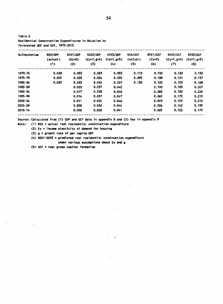
54

Table 6 Residential Construction Expenditures in Relation to Forecasted GOP and GCF, 1970-2015

Quinquennium REX/GOP REX1/GDP REX2/GDP REX3/GDP REX/GCF REX1/GCF REX2/GCF REX3/GCF (actual) (Ey=0) <Ey=1,g=4) (Ey=1,g=5) (actual) (Ey=0) (Ey=1#g=4) (Ey=1,g=5) <1> (2) <3) (4) (5) (6) (7) (8)

1970-74 0.028 0.033 0.033 0.033 0.113 0.132 0.132 0.132 1975-79 0.025 0.028 0.034 0.035 0.095 0.108 0.131 0.137 1980-84 0.029 0.023 0.034 0.037 0.130 0.103 0.153 0.168 1985-89 0.020 0.037 0.042 0.100 0.180 0.207 1990-94 0.017 0.038 0.046 0.083 0.182 0.220 1995-99 0.014 0.037 0.047 0.065 0.172 0.219 2000-04 0.011 0.035 0.046 0.049 0.159 0.212 2005-09 0.008 0.032 0.044 0.036 0.142 0.199 2010-14 0.006 0.028 0.041 0.025 0.122 0.179

Source: Calculated from (1) GOP and GCF data in appendix 8 and (2) Rex in appendix 9 Note: (1) REX = actual real residential construction expenditure

(2) Ey = income elasticity of demand for housing (3) g 9 growth rate of per capita GDP (4) REX1-REX3 a predicted real residential construction expenditure

under various assumptions about Ey end g (5) GCF 3 real gross capital formation

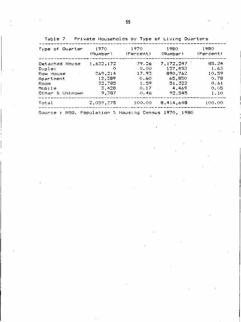
55

Table 7 P r i v a t e Households by Type o-f L i v i n g Q u a r t e r s

Type o-f Quarter 1970 1970 1980 1980 (Number) (Percent) (Number) (Percent)

Detached House 1,632,172 79.26 7,172.247 85-24 Dup1 ex 0 0. 00 137,453 1.63 Row House 369,214 17.93 890,762 10.59 Apartment 12,389 0. 60 65,850 0. 78 Room 32,785 1.59 51,322 0 ..61 Mob i 1 e 3 < 428 0.17 4,469 0. 05 Other & Unknown 9,387 0. 46 92.545 1.10

T o t a l 2,059,375 100-00 8,414,648 100.00

Source : NS0- P o p u l a t i o n & Housing Census 1970, 1980

56

Table 8 P r i v a t e Households by Type of Construct!on Mater i a i s

Construct i on 1970 1970 1 980 1980 Materi a l s (Number) (Percent) (Number > (Percent)

Cemen t o-f Br i c k 124,102 6.06 534,039 6. 35 Wood and Cement 78,780 3.85 509,973 6. 06 Wood 1,349,617 65- 95 5,888,114 69. 97 Local Materi a l s 413,865 20. 22 1,273,284 15. i3 Reused Materi a l s 62,282 3.04 74,332 0. SB Unknown 17,914 0. 33 134,967 1 - 60

Tot a l 2,046,560 100-00 8,414,709 100.00

Source : NS0. P o p u l a t i o n & Housing Census 1970, 1980

57

Table 9 P r i v a t e Households by Sources o-f Water Supply, L i g h t i n g , Type o-f Bathroom and Kitch e n

Type 1970 1970 1980 1980 Type (Number > (Percent (Number) (Percent

Source o-f Water Sup pi y ,046,560 100-00 8 ,410,989 100.00 Pi ped i n s i d e 436,677 21 . 34 1 ,305,437 15.52 Pi ped o u t s i de 166,185 8, 12 286,180 3. 40 Others & U n k no wn 1 ,443,698 70.54 6 ,319,372 G 1 . 08

L i g h t i n g ,046,560 100-00 3 ,411,119 100.00 E l e c t r i c L i g h t i n g 766,633 37. 46 3 ,615,019 42. 93 Pressure Lamp 0 0 - 00 57,327 0. 68 O i l Lamp o 0 - 00 4 ,608,031 54-78 Other & Unknown 1 ,279,927 62 n 54 130,742 1-55

Bathrooms 0 0- 00 8 ,411,050 100.00 E:; c 1 u s i ve 0 0. 00 T ,213,187 38.20 Shared 0 0, 00 224,406 2. 67 Terrace/Verandah 0 0. 00 ,233,781 26.56 Others & Unknown 0 0. 00 2 ,739,676 32.57

T o i 1 e t F a c i I i t y ,046,560 100.00 8 ,410,940 100.00 F.l ush , E:<cl u s i ve 41,470 2. 03 318,627 3.79 F l u s h , Shared 6,735 0. 33 37,810 0-45 Moulded Bucket 777,288 37. 98 ,838,810 45.64

L a t r i ne, E x c l u s i ve Moulded Bucket 143,420 7.01 394,648 4.69

L a t r i ne, Shared P i t 0 0. 00 790,264 9. 40 Others & Unknawn 1 ,077,647 52. 66 ,030,781 36. 03

Source : NS0. P o p u l a t i o n & Housing Census 1970, 1980

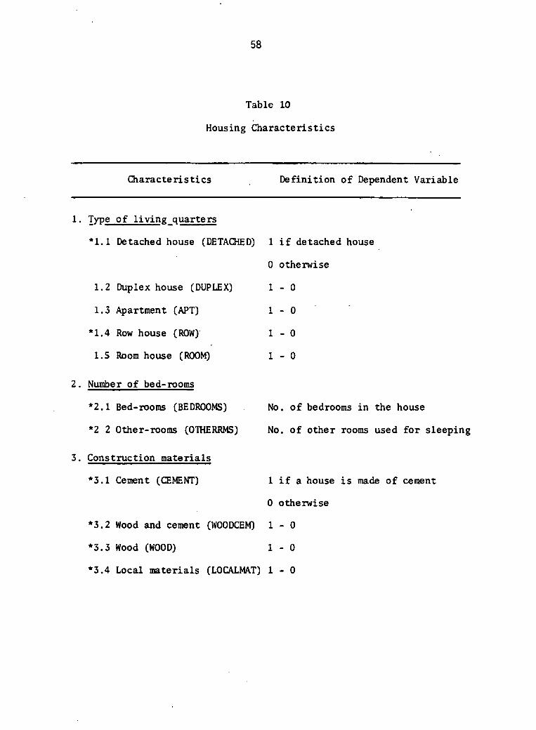
58

Table 10

Housing Characteristics

Characteristics Definition of Dependent Variable

1 • Type of living quarters

*1.1 Detached house (DETACHED) 1 i f detached house

1.2 Duplex house (DUPLEX)

1.3 Apartment (APT)

*1.4 Row house (ROW)

1.5 Room house (ROOM)

2. Number of bed-rooms

*2.1 Bed-rooms (BEDROOMS)

*2 2 Other-rooms (01HERRMS)

3. Construction materials

*3.1 Cement (CEMENT)

*3.2 Wood and cement (WOODCEM)

*3.3 Wood (WOOD)

0 otherwise

1 - 0

1 - 0

1 - 0

1 - 0

No. of bedrooms in the house

No. of other rooms used for sleeping

1 i f a house is made of cement

0 otherwise

1 - 0

1 - 0

3.4 Local materials (LOCALMAT) 1

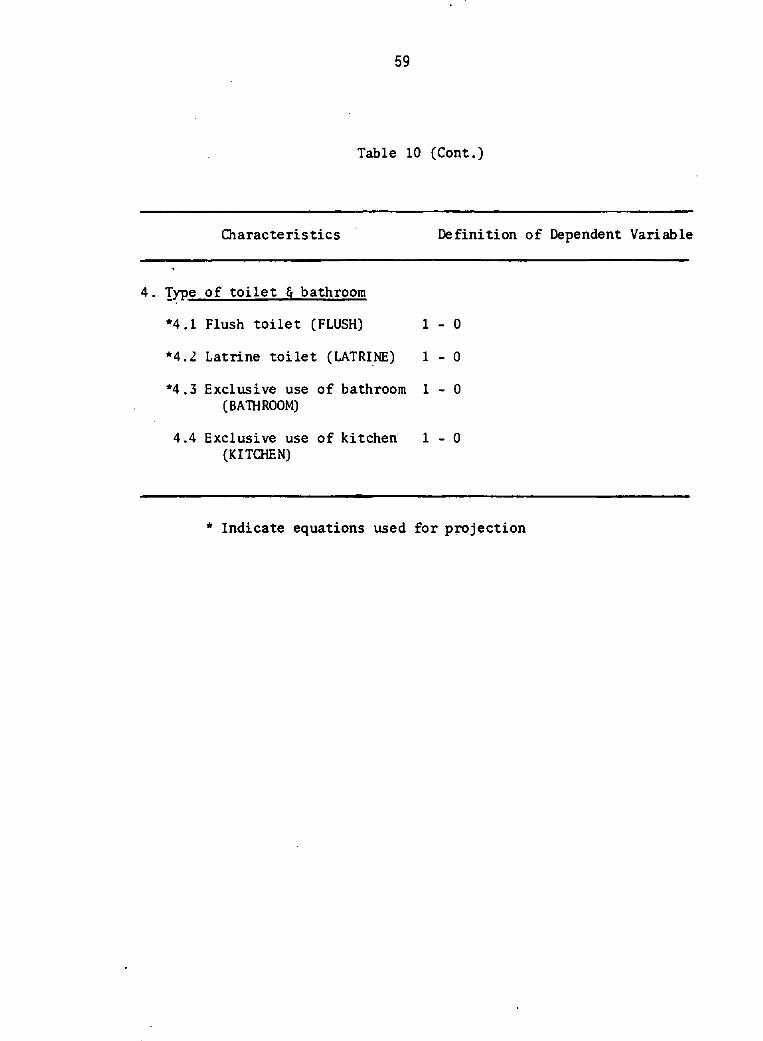
59

Table 10 (Cont.)

Characteristics Definition of Dependent Variable

4. Type of toilet 5 bathroom

*4.1 Flush toilet (FLUSH) 1 - 0

*4.2 Latrine toilet (LATRINE) 1 - 0

*4.3 Exclusive use of bathroom 1 - 0 (BATHROOM)

4.4 Exclusive use of kitchen 1 - 0 (KITCHEN)

* Indicate equations used for projection

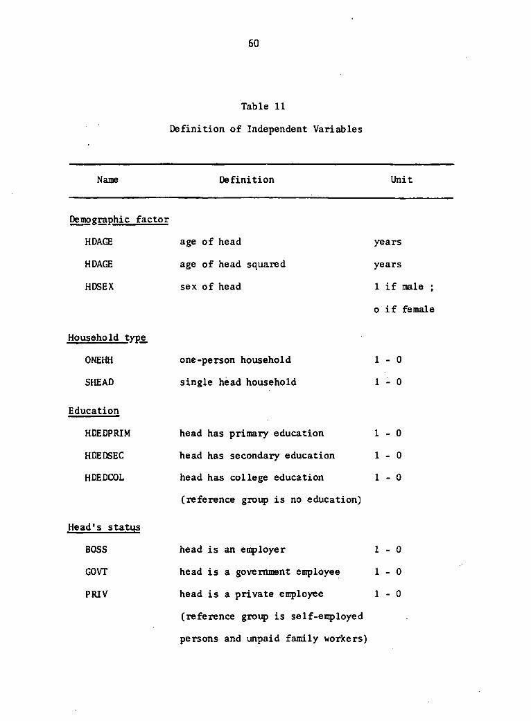
60

Table 11

Definition of Independent Variables

Name Definition Unit

Demographic factor

HDAGE

HDAGE

HDSEX

Household type

ONEHH

SHEAD

Education

HDEDPRIM

HDEDSEC

HDEDCOL

Head's status

BOSS

GOVT

PRIV

age of head

age of head squared

sex of head

one-person household

single head household

head has primary education

head has secondary education

head has college education

(reference group is no education)

head is an employer

head is a government employee

head is a private employee

(reference group is self-employed

persons and unpaid family workers)

years

years

1 i f male ;

o i f female

1 -

1 -

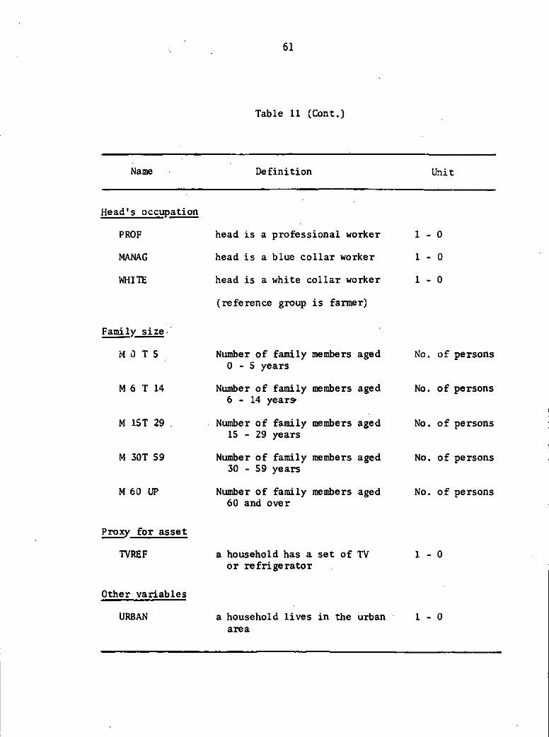
61

Table 11 (Cont.)

Name Definition Unit

Head's occupation

PROF

MANAG

WHITE

Family size-

MO T 5

M 6 T 14

M 15T 29

M 30T 59

M 60 UP

Proxy for asset

TVREF

head is a professional worker

head is a blue collar worker

head is a white collar worker

(reference group is farmer)

Number of family members aged 0 - 5 years

Number of family members aged 6 - 1 4 years*

Number of family members aged 15 - 29 years

Number of family members aged 30 - 59 years

Number of family members aged 60 and over

a household has a set of TV or refrigerator

1 - 0

1 - 0

1 - 0

No. of persons

No. of persons

No. of persons

No. of persons

No. of persons

1 - 0

Other variables

URBAN a household lives in the urban area

1 - 0

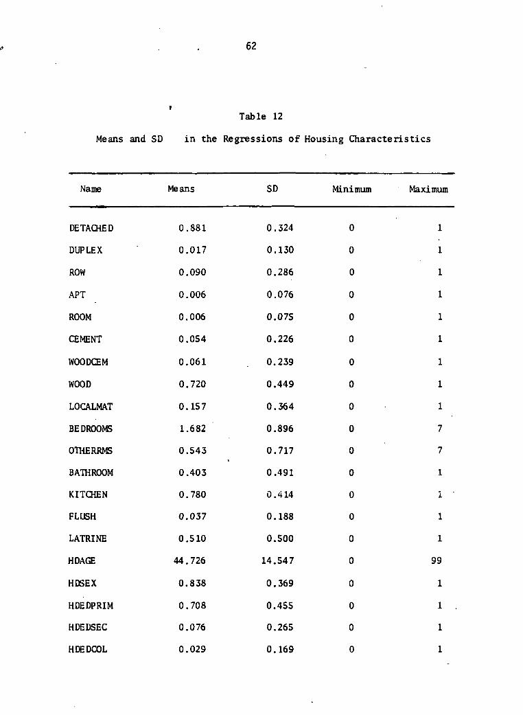
62

Table 12

Means and SD in the Regressions of Housing Characteristics

Name Means SD Minimum Maximum

DETACHED 0.881 0.324 0 i

DUPLEX 0.017 0.130 0 i

ROW 0.090 0.286 0 i

APT 0.006 0.076 0 i

ROOM 0.006 0.07S 0 i

CEMENT 0.054 0.226 0 i

WOODCEM 0.061 0.239 0 i

WOOD 0.720 0.449 0 i

LOCALMAT 0.157 0.364 0 i

BEDROOMS 1.682 0.896 0 7

OTHERRMS 0.543 0.717 0 7

BATHROOM 0.403 0.491 0 1

KITCHEN 0.780 0.414 0

FLUSH 0.037 0.188 0 1

LATRINE 0.510 0.500 0 1

HDAGE 44.726 14.547 0 99

HDSEX 0.838 0.369 0 1

HDEDPRIM 0.708 0.455 0 1

HDEDSEC 0.076 0.265 0 1

HDEDCOL 0.029 0.169 0 1

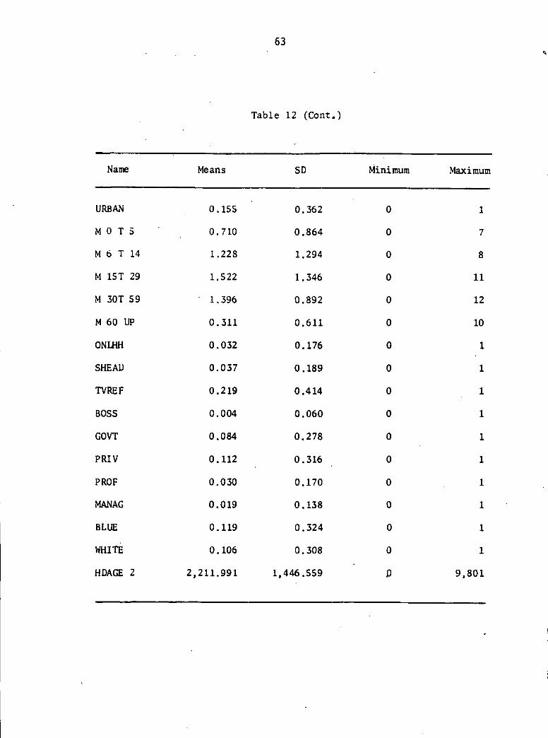
63

Table 12 (Cont.)

Name Means SD Minimum Maximum

URBAN

M 0 T 5

M 6 T 14

M 15T 29

M 30T 59

M 60 UP

ONLHH

SHEAD

TVREF

BOSS

GOVT

PRIV

PROF

MANAG

BLUE

WHITE

HDAGE 2

0.155

0.710

1.228

1.522

1.396

0.311

0.032

0.037

0.219

0.004

0.084

0.112

0.030

0.019

0.119

0.106

2,211.991

0.362

0.864

1.294

1.346

0.892

0.611

0.176

0.189

0.414

0.060

0.278

0.316

0.170

0,138

0.324

0.308

1,446.559

1

7

8

11

12

10

9,80

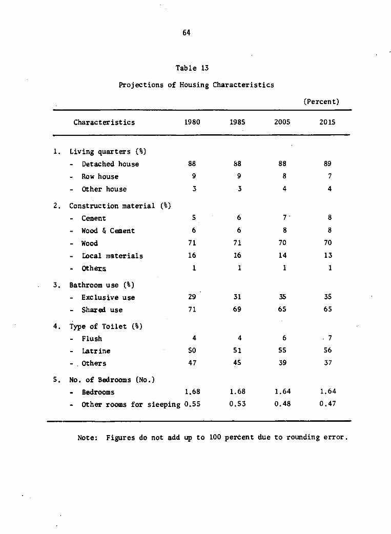
64

Table 13

Projections of Housing Characteristics

(Percent)

Characteristics 1980 1985 2005 2015

1. Living quarters (%) - Detached house 88 - Row house 9

- Other house 3

2. Construction material (%} - Cement 5

- Wood 5 Cement 6

- Wood 71

Local materials 16

- Others 1

3. Bathroom use (%) - Exclusive use 29 - Shared use 71

4. Type of Toilet (%) - Flush 4 - Latrine 50 - . Others 47

5. No. of Bedrooms (No.) - Bedrooms 1.68 - Other rooms for sleeping 0.55

88 9 3

6

6 71 16

1

31 69

4 51 45

1.68 0.53

88 8 4

7 *

8 70 14

1

35 65

6 55 39

1.64

0.48

89 7 4

8

8 70 13

1

35 65

• 7 56 37

1.64 0.47

Note: Figures do not add up to 100 percent due to rounding error.

65

Table 14 Di s t r i but i on o-f Loan by Economi c S e c t o r s (31 December 1985)

(Percent)

Sector Commercial Bank Finance Companies

A g r i c u l t u r e and Mining 8 „ 0 1-7 Industry 23. 1 23. 9 Construct i on 5.5 5.3 Real E s t a t e Development 3-6 11.1 F o r e i g n Trade 14. 9 6. 0 Domestic Trade 23, 0 15.2 F i nanci a l I n s t i tut i ons 6, 2 10.6 S e r v i ce 5. 1 9.0 Mortgage Loan 2.8 Rental Purchase 5. 4 13. 4 Others 2.0 1.0

T o t a l 100- 0 1 00. 0

Source : Finance Unit , Bank o-f Thai 1 and

66

Table 15 Source o-f Housing Mortgage Loan

Inst i t u t i ons 1981 1983 1984

Commerci a l Bank 7,063 12,733 16,998 Bank o-f Housing 6,497 6 ,337 7,846 C r e d i t Companie 1 ,481 1 ,867 2,763 Nat i a n a l Housin 1 , 402 1 ,675 1 ,474 Insurance Compa 565 875 1 ,390 C r e d i t F o n c i e r s 482 516 388 Others 646 647 784

Source : (1) Finance Unit , Bank o-f Thai 1 and (2) Praisart Tan gnat i tham , F i n a n c i a l

I n s t i t u t i o n s i n some c o u n t r i es and I m p l i c a t i o n s on the Housing C r e d i t P o l i c y i n T h a i l a n d , r e s e a r c h r e p o r t , F a c u l t y of Economi c s , Thammasat U n i v e r s i t y ,1987 n

Note : e = estimated by P r a s a r t Tangmatitham.

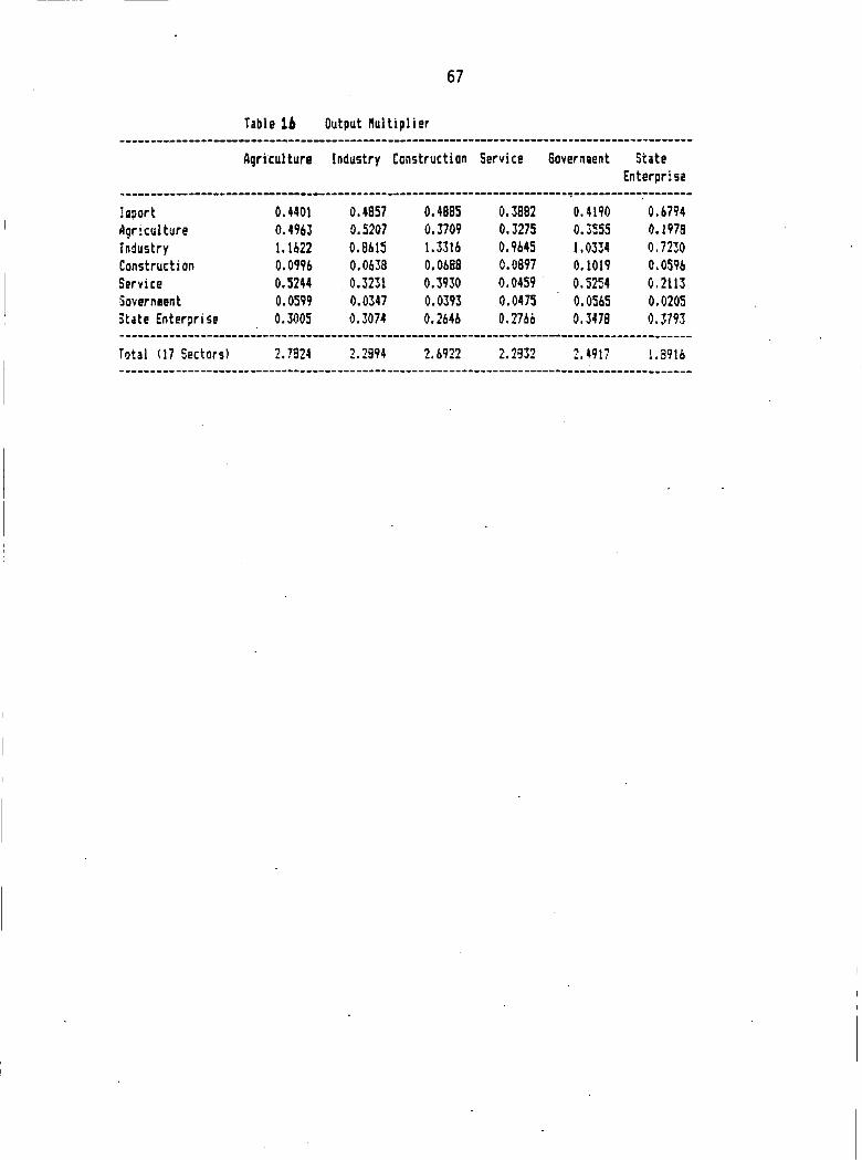
67

Table 16 Output Mul t ip l ie r

Agriculture Industry Construction Service Sovernaent State Enterprise

I aport 0.4401 0.4857 0.4B85 0.3882 0.4190 0.6794 Agriculture 0.4963 0.5207 0.3709 0.3275 0.o555 0.1978 Industry 1-1422 0.8615 1.3316 0.9645 1.0334 0.7230 Construction 0.0996 0.0638 0.0688 0.0897 0.1019 0.0596 Service 0.5244 0.3231 0.3930 0.0459 0.5254 0,2113 Government 0.0599 0.0347 0.0393 0.0475 0.0565 0.0205 State Enterprise 0.3005 0.3074 0.2646 0.2766 0.3478 0.3793

Total (17 Sectors) 2.7324 2.2994 2.6922 2.2332 2.4917 1.3916

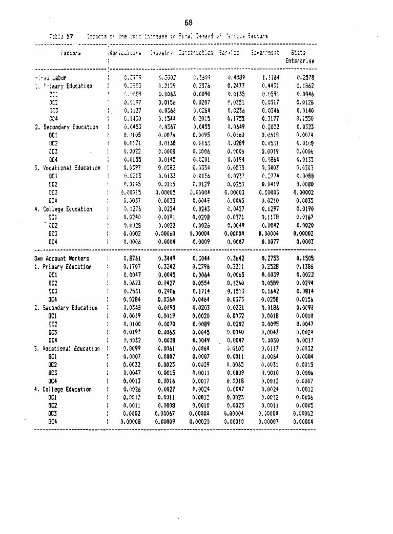
68

T i b U 17 ; -a; ac ts Dne "jr-i: I in ~ * • r * i r - 5 * Is-: t a r s

Factors i

: - G - i t r v : *-=t j c t i c r , •3GV2,TaS-lt S t a t s

Enterprise

Labor 0.3002 0.3609 0.4089 1.1164 0.2578 t; : - ; *a ry Education I 0.15:3 0.2129 0.2576 0.2477 0.4431 0.1362

! C. -::059 0.0063 0.0090 0.0135 0.0591 0.0046 0C2 y.0197 0.0156 0.0207 0.0351 0.0317 0,0126

!. 0.1137 0.0366 0.0264 0.0236 0.0346 0.0140 CC4 ! 0 .14$) 0.1544 0.2015 0.1755 0.3177 0.1550

2. Secondary Education ! 0.0453 0.0367 0.0455 0.0649 0.2032 0.0323 0C1 0.0105 0.0076 0,0095 0.0160 0.0613 0.0074 0C2 i 0.0171 0.0138 0.0153 0.0289 0.0531 0.0108 nr-T 0.0022 0.0008 0.0006 0.0006 0.0019 C.0006 QC4 i 0.0155 0.0145 o.cz-oi 0.0194 0.0864 0.0135

3, Vocational Education 0.0397 0.0282 0.0334 0.0535 0.3403 0.0203 QC1 i 0.0213 0,0133 0.C156 0.023? 0.2774 0,0068 0E2 ' 0.5115 0.0129 0.0253 0.0419 0.0080 0L3 0.00015 0.00005 0.00004 0.00003 0.00003 0.00002 0C4 0.0037 0,0033 0,0049 0.0045 0.0210 0.0035

4. Collage Education ; 0.0276 0.0224 0.0243 0.0427 0.1297 0.0190 0C1 0.0240 0.0191 0.0203 0.0371 0.U7B 0.0167

" 0C2 0,0025 0.0023 0,0026 0.0049 0.0042 0.0020 0C3 0.0002 0.00060 0.00004 0.00C04 0.00004 0.00002 QC4 0.0006 0.0004 0.0009 0.0007 0.0077 0.0003

Oxn Account Workers 0.8761 0.3449 0.3044 0.3642 0.2753 0.1505 1. Primary Education 0,1707 0.3242 0.2796 0.3211 0.2528 0.1386

OCi 0.0047 0.0045 0.0064 0.0065 0.0039 0.0022 QC2 0.0623 0.0427 0.0554 0.1260 0.0589 0.0294 0C3 0.7531 0.2406 0.1714 0.1513 0.1642 O.0814 0C4 0.0284 0.0364 0.0464 . 0.0373 0.0258 0.0156

2. Secondary Education 0.0343 0.0190 0.0203 0.0321 0.0166 0.0093 OCI 0.0019 0.0019 0,0020 0.0032 0.0018 0,0010 0C2 0.0100 0.0070 0.0089 0.0202 0.0095 0.0047 QC3 0.019? 0.0063 0.0045 0.0040 0.0043 5.0024 0C4 0.0032 0.0038 0.0049 0.0047 0.0030 0.0017

3, Vocational Education 0.0099 0.0061 0,0064 0.0103 0.0117 0.0032 OCI 0.0007 0.0007 0.0007 0,0011 0.0064 0.C004 0C2 0.0032 0.0023 0.0029 0.0065 0.0031 0.0015 QC3 0.0047 0.0015 0.0011 0.0009 0.0010 0.0006 0C4 0.0013 0.0016 0.0017 0.0018 0.0012 0.0007

4, College Education 0.0026 0.0027 0.0024 0.0047 0.0024 0.0012 OCI 0.0012 0.0011 0.0012 0.0023 0.0012 0.0006 012 0,0011 0.0008 0.0010 0.0023 0.0011 0.0005 0C3 0.0002 0.00067 0.00004 0.00004 0.00004 0.00002 0C4 0.00008 0.00009 0.00020 0.00010 0.00007 0.00004

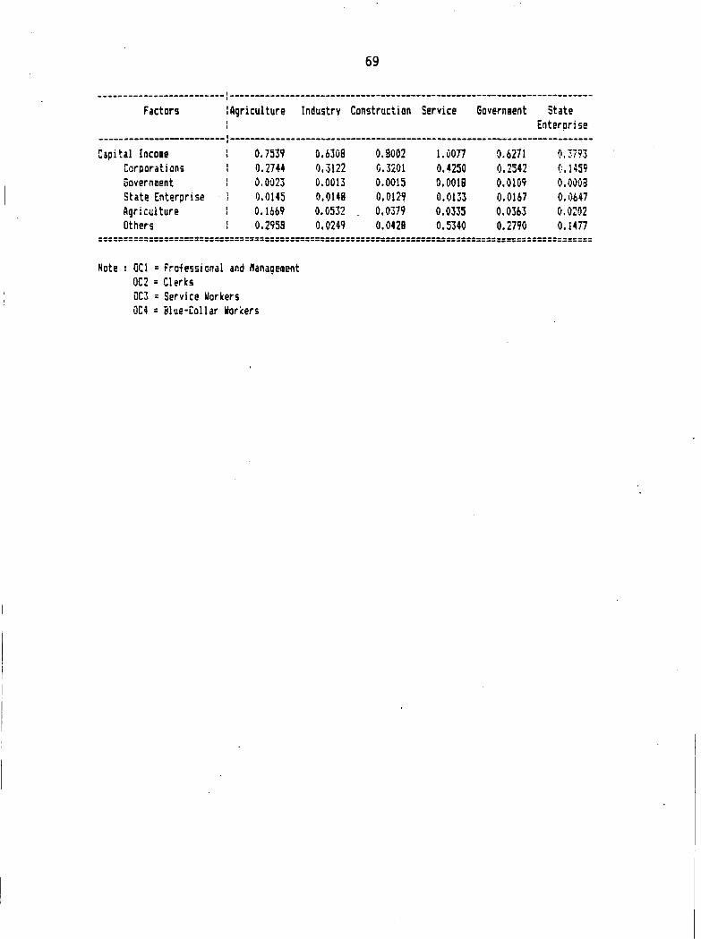
69

Factors Agriculture Industry Construction Service Governaent State Enterprise

Capital Incoae 0.7539 0.6308 0.8002 1.0077 0.6271 0.3793 Corporations 0.2744 0,3122 0.3201 0.4250 0.2542 0.1459 Sovernaent 0.0023 0.0013 0.0015 0.0018 0.0109 0.0003 State Enterprise 0.0145 0.0148 0.0129 0.0133 0.0167 0.0647 Agriculture 0.1669 0.0532 0.0379 0.0335 0,0363 0.0202 Others 0.2958 0.0249 0.0428 0.5340 0.2790 0.1477

:============: ============= ============ ============

Note : GC1 = Professional and Nanageaent 0C2 = Clerics QC3 = Service Workers 0C4 = Blue-Collar Workers

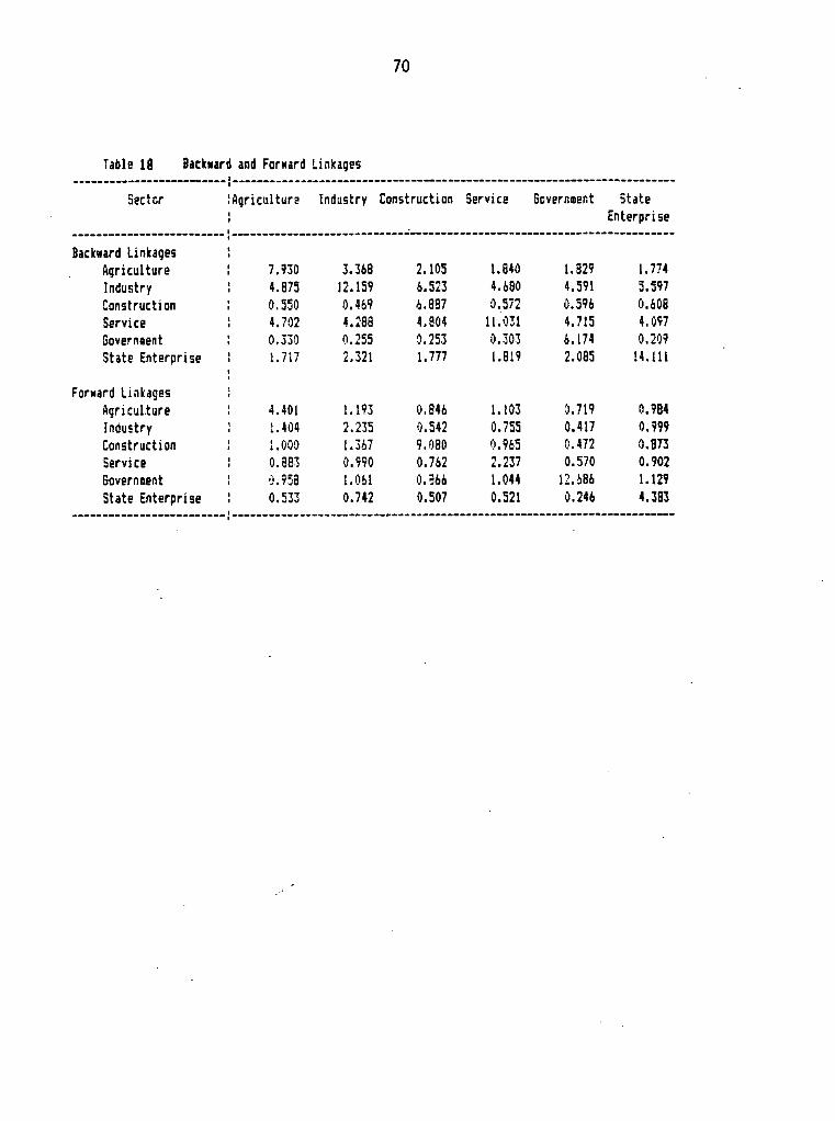
70

Table 18 Backward and Forward Linkages

Sector Agriculture Industry Construction Service Scvernnent State Enterprise

Backward Linkages Agriculture 7.930 3.368 2.105 1.840 1.329 1.774 Industry 4.875 12.159 6.523 4.680 4.591 5.597

Construction 0.550 0.469 4.887 0.572 0.596 0.608 Service 4.702 4.288 4.804 11.031 4.715 4.097 Sovernaent 0.330 0.255 0.253 0.303 6.174 0.209 State Enterprise 1.717 2.321 1.777 1.819 2.085 14.111

Forward Linkages Agriculture 4.401 1.193 0.846 1.103 0,719 0.984 Industry 1.404 2.235 0.542 0.755 0.417 0.999 Construction 1.000 1.367 9,030 0.965 0.472 0,873 Service 0.8B3 0.990 0.762 2.237 0.570 0.902 Governnent 0.958 1.061 0.566 1.044 12.686 1.129

State Enterprise 0.533 0.742 0.507 0.521 0.246 4.383

Figure 1 - A Housing Inventories (Hi)

1 1 1 1 1 1 1 1 \ ~ 1 1 1 1 1

1950 1955 1960 1965 1970 1975 1980 1985 1990 1995 2000 2005 2010 201

Year

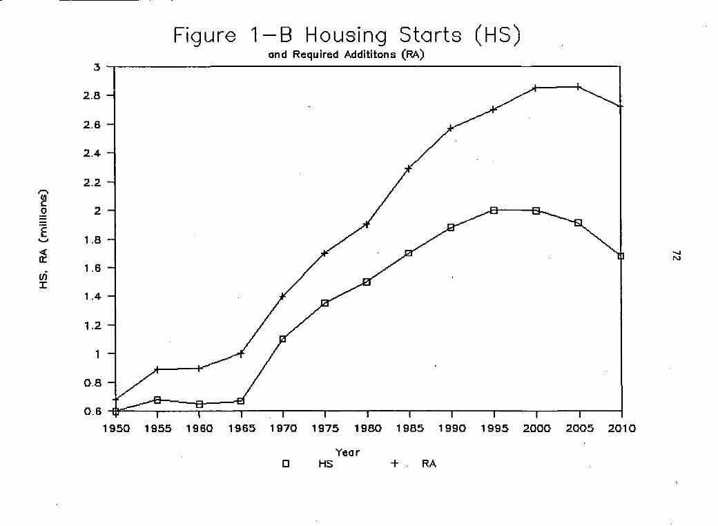
Figure 1—B Housing Starts (HS) and Required Addititons (RA)

1950 1955 1960 1965 1970 1975 1980 1985 1990 1995 2000 2005 2010

Year • HS + . RA

Year

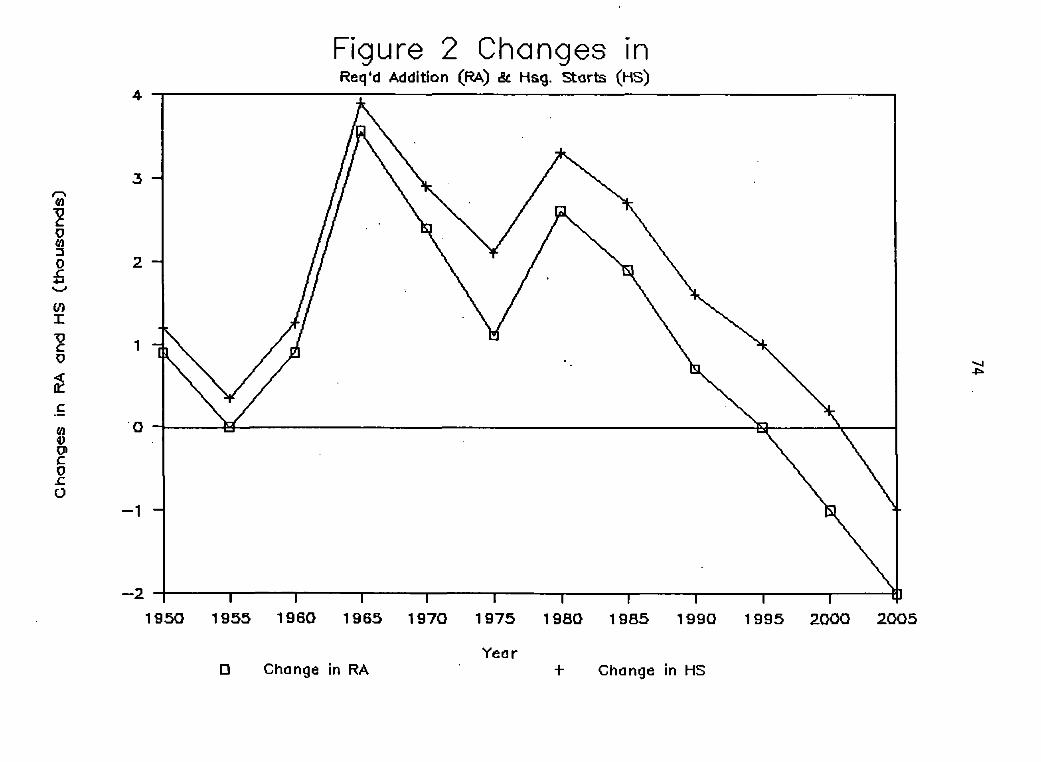
Figure 2 Changes in Req'd Addition (RA) & Hsg. Starts (HS)

1950 1955 1960 1965 1970 1975 1980 1985 1990 1995 2000 2005

Year • Change in RA + Change in HS

Figure 3 Housing Starts/Housing Pop 0.076

Q_ X N (J) x

0.074 H

0.072 H

0.06 H

0.058 H

0.056 H

0.054 H

0.052 H

0.05

1 1 1 1 1 1 1 1 1 60-65 65-70 70-75 75-80 80-85 85-90 90-95 95-00 00-05 05-10 1 0-15

Period

Figure 4 Changes in Residential-Construction Expenditure (CX)

70 -i

75—79 80—84 85—89 90—94 95—99 00-04 05—10 10—14

• C Rex1 Period

+• C Rex2 O C Rex3

THE EAST-WEST CENTER is a p u b l i c , nonpro f i t educa t i ona l inst i tu­t ion w i t h an in te rna t iona l boa rd of governors . S o m e 2,000 research fe l lows, g raduate s tudents , a n d p ro fess iona ls in bus i ­ness and gove rnmen t each year work w i t h the Cen te r ' s in te rna­t iona l staff in coopera t i ve study, t ra in ing , a n d research . They examine ma jor issues re lated to p o p u l a t i o n , resources a n d de­v e l o p m e n t , the e n v i r o n m e n t , cu l tu re , a n d c o m m u n i c a t i o n in A s i a , the Paci f ic, and the U n i t e d States. The C e n t e r was estab­l ished in 1960 by the U n i t e d States C o n g r e s s , w h i c h p rov ides p r inc ipa l f u n d i n g . S u p p o r t a lso c o m e s f rom more than 20 A s i a n and Pacif ic gove rnmen ts , as we l l as pr ivate agenc ies a n d c o r p o ­rat ions.

Situated on 21 acres adjacent to the Universi ty of Hawai i 's M a n o a C a m p u s , the Cen te r ' s fac i l i t ies i n c l u d e a 300-room o f f i ce bu i l d ­ing h o u s i n g research a n d admin is t ra t i ve o f f i ces for an in terna­t iona l staff of 250, three res idence hal ls for par t ic ipants , a n d a con fe rence cen te r w i t h mee t i ng r o o m s e q u i p p e d to p rov ide s imu l t aneous t rans la t ion and a c o m p l e t e range of aud iov i sua l serv ices.

THE EAST-WEST POPULATION INSTITUTE, es tab l i shed as a un i t of the East-West C e n t e r in 1969, carr ies ou t mu l t i d i sc i p l i na ry research , t ra in ing, a n d related act iv i t ies in the f ie ld of p o p u l a ­t i on , p lac ing e m p h a s i s o n e c o n o m i c , soc ia l , p sycho log i ca l , a n d env i ronmen ta l aspects of p o p u l a t i o n p r o b l e m s in A s i a , the Pa­ci f ic , and the U n i t e d States.