processes

Article

Research on the Dynamic Responses of Simply SupportedHorizontal Pipes Conveying Gas-Liquid Two-Phase Slug Flow

Gang Liu 1,2,3,4, Zongrui Hao 1,2,3,* , Yueshe Wang 4 and Wanlong Ren 1,2,3

�����������������

Citation: Liu, G.; Hao, Z.; Wang, Y.;

Ren, W. Research on the Dynamic

Responses of Simply Supported

Horizontal Pipes Conveying

Gas-Liquid Two-Phase Slug Flow.

Processes 2021, 9, 83. https://

doi.org/10.3390/pr9010083

Received: 15 November 2020

Accepted: 29 December 2020

Published: 2 January 2021

Publisher’s Note: MDPI stays neu-

tral with regard to jurisdictional clai-

ms in published maps and institutio-

nal affiliations.

Copyright: © 2021 by the authors. Li-

censee MDPI, Basel, Switzerland.

This article is an open access article

distributed under the terms and con-

ditions of the Creative Commons At-

tribution (CC BY) license (https://

creativecommons.org/licenses/by/

4.0/).

1 Institute of Oceanographic Instrumentation, Qilu University of Technology (Shandong Academy of Sciences),Qingdao 266100, China; liu-g@qlu.edu.cn (G.L.); renwl@qlu.edu.cn (W.R.)

2 Shandong Provincial Key Laboratory of Marine Monitoring Instrument Equipment Technology,Qingdao 266100, China

3 National Engineering and Technological Research Center of Marine Monitoring Equipment,Qingdao 266100, China

4 State Key Laboratory of Multiphase Flow in Power Engineering, Xi’an Jiaotong University,Xi’an 710049, China; wangys@mail.xjtu.edu.cn

* Correspondence: haozr@qlu.edu.cn

Abstract: The dynamic responses of simply supported horizontal pipes conveying gas-liquid two-phase slug flow are explored. The intermittent characteristics of slug flow parameters are mainlyconsidered to analyze the dynamic model of the piping system. The results show that the variations ofthe midpoint transverse displacement could vary from periodic-like motion to a kind of motion whoseamplitude increases as time goes on if increasing the superficial gas velocity. Meanwhile, the dynamicresponses have certain relations with the vibration acceleration. By analyzing the parameters in thepower spectrum densities of vibration acceleration such as the number of predominant frequenciesand the amplitude of each peak frequency, the dynamic behaviors of the piping system like periodicitycould be calculated expediently.

Keywords: simply supported pipe; two-phase slug flow; intermittent; dynamic responses

1. Introduction

Fluid-conveying piping systems have been continually adopted in various processesof modern chemical engineering. It is crucial to guarantee the safety of the process oftransporting materials. As is known, instability of the piping system may occur due tothe vibrations induced by the internal flow, which has drawn the attention of numerousscholars. The explorations of the dynamics of the fluid-conveying piping system since the1880s have been summarized systematically by Paidoussis and Issid [1].

It has been noted that with a sufficiently large constant flow velocity, divergence orflutter could happen for the piping system. In addition, for harmonically varying flowvelocity, some complex dynamical behaviors like quasi-periodic may take place, whichwould bring more damages to the operation of the pipeline, which have been furtherconfirmed by the researches of Ariaratnam and Namachchivaya [2] and Jin and Song [3].Pipes conveying single-phase fluid have been researched deeply by scholars including theabove several experts.

Actually, piping systems conveying two-phase flow may have a wider range ofapplications in science and engineering [4]. Alamian et al. [5] established a mathematicalmodel to explore the instantaneous flow inside the gas pipelines. They discussed the effectsof boundary conditions particularly. Goodarzi et al. [6] and [7] investigated the Erosionphenomenon in pipes conveying two-phase flow. Pourfattah et al. [8] carried out the two-phase flow simulation of the heat transfer characteristics of the manifold microchannel heatsink. Almasi et al. [9] introduced an SPH method to explore the multiphase phenomenon.Shadloo et al. [10] discussed the pressure drop which is one significant parameter that

Processes 2021, 9, 83. https://doi.org/10.3390/pr9010083 https://www.mdpi.com/journal/processes

Processes 2021, 9, 83 2 of 13

would define the two-phase system in the pipe by the artificial neural networks. The effectsof pressure drop on the dynamics of the piping system may be necessary to be explored inthe future.

Due to the different proportions of flow rates of the two phases, several typical flowpatterns could be observed in the pipes [11]. Among these flow regimes, slug flow hasreceived more attention due to its intermittent features [12]. For instance, Dukler andHubbard [13] and Zhang et al. [14] have developed their own models to calculate typicalslug flow parameters. According to their researches, local slug flow parameters such asthe velocities of gas and liquid would always vary with position and time, which wouldmake the vibration of the slug flow piping system more complex. Riverin et al. [15],Cargnelutti et al. [16], Liu et al. [17], and Giraudeau et al. [18] indicated that the largestvibrations appeared in the slug flow system. An and Su [19] established a differentialequation for a slug flow conveying riser subjected to vortex-induced force. They analyzedthe variation of the transverse displacement for the riser with different flow rates.

Recently, the dynamics of piping systems conveying two-phase flow have been attract-ing the attention of scholars. Ebrahimi-Mamaghani et al. [20] emphasized the significanceof flow parameters for the dynamic behaviors of the vertical piping system conveyingtwo-phase flow. Sazesh and Shams [21] indicated the stabilities of the piping systemcould be affected markedly by time-varying phenomena like pulsating two-phase flow.Extraordinarily, some scholars paid attention to the piping system conveying two-phaseslug flow. Khudayarov et al. [22] explored the relationships between some typical slugparameters such as the length of the gas bubble zone and the dynamic behaviors of thepiping system. Zhu et al. [23] suggested that for a piping system conveying two-phase slugflow, the dynamic responses would be related to the intermittent characteristics of the slugflow. Cabrera-Miranda and Paik [24] pointed out that two significant parameters includingthe slugging frequencies and slug lengths should be deeply considered in the process ofdesign for the piping system. It could be noted that the intermittent characteristics of slugflow leading to the dynamics of the piping system are extremely complicated.

Based on most scholars who are devoted to analyzing the dynamics of simply sup-ported pipes conveying fluids, the flow parameters such as fluid velocity varying with theposition of the pipe should be calculated. For the pipes conveying single-phase flow, thefluid velocity was supposed as constant along the pipe or written as a ripple value.

Nevertheless, for pipes conveying slug flow, the local flow velocity at every fixedcross section over the time of the passage of a slug unit would be equal to the velocity inthe film zone for the case that a gas bubble passes the cross section at one moment whilewould be equal to the velocity in the slug zone for the case that a liquid slug passes thecross section at another moment, which was considered in this work. Then we can analyzethe dynamics of the piping system corresponding to various working conditions of slugflow. While few scholars have analyzed the local flow parameters varying with time andposition to explore the pipes conveying slug flow.

In general, the piping system conveying slug flow deserves deep concern with fewscholars exploring the dynamic responses, which is the main objective of this study. Thedynamic model will be established in Section 2. Galerkin’s method is employed to discretehigher-order differential equations while the Runge Kutta method is introduced to obtainthe variations of vibration parameters. Then the dynamic responses of the piping systemunder different conditions will be discussed in Section 3. Finally, some significant findingswill be narrated in Section 4.

2. Materials and Methods

A simply supported pipe conveying gas-liquid two-phase slug flow is depictedin Figure 1. It can be easily observed that the slug flow consists of several successiveslug units.

Processes 2021, 9, 83 3 of 13Processes 2021, 9, x FOR PEER REVIEW 3 of 13

Figure 1. Schematic of a simply supported pipe conveying two-phase slug flow.

As shown in Figure 2, a gas bubble and a liquid slug would constitute one stable slug

unit. It is assumed that the sectional area of the inner pipe is Ai and the volume flow rate

is Q. Then the superficial gas velocity uSG and superficial liquid velocity uSL are obtained

by:

𝑢𝑆𝐺 =𝑄𝐺

𝐴𝑖, 𝑢𝑆𝐿 =

𝑄𝐿

𝐴𝑖 (1)

Figure 2. Schematic of a stable slug unit.

Referring to the work of Wang [25], the mathematical model of a slug flow conveying

pipe could be written as:

𝐸𝐼𝜕4𝑦

𝜕𝑥4+ 2[𝑚𝐿(𝑥, 𝑡)𝑢𝐿(𝑥, 𝑡) + 𝑚𝐺(𝑥, 𝑡)𝑢𝐺(𝑥, 𝑡)]

𝜕2𝑦

𝜕𝑡𝜕𝑥+ [𝑚𝐿(𝑥, 𝑡)𝑢𝐿

2(𝑥, 𝑡) + 𝑚𝐺(𝑥, 𝑡)𝑢𝐺2 (𝑥, 𝑡)]

𝜕2𝑦

𝜕𝑥2

+ [𝑚𝐿(𝑥, 𝑡) + 𝑚𝐺(𝑥, 𝑡) + 𝑚𝑃]𝜕2𝑦

𝜕𝑡2− [

𝐸𝐴𝑖

2𝐿∫ (

𝜕𝑦

𝜕𝑥)

2

𝑑𝑥𝐿

0

]𝜕2𝑦

𝜕𝑥2= 0

(2)

The implications of the parameters of the above model could be found in the paper of

Liu and Wang [26].

The transient pattern of slug flow at two typical moments is shown in Figure 3. It

could be noted that uL(x,t) = uLF at t = t1 as shown in Figure 3a while uL(x,t) = uS at t = t2 as

depicted in Figure 3b, which means that uL(x,t) is the function of the coordinate x and the

time t. Then it is pivotal to obtain the variations of flow parameters with x and t. to analyze

Equation (2), which could be found in Liu and Wang [26].

Figure 1. Schematic of a simply supported pipe conveying two-phase slug flow.

As shown in Figure 2, a gas bubble and a liquid slug would constitute one stable slugunit. It is assumed that the sectional area of the inner pipe is Ai and the volume flow rate isQ. Then the superficial gas velocity uSG and superficial liquid velocity uSL are obtained by:

uSG =QGAi

, uSL =QLAi

(1)

Processes 2021, 9, x FOR PEER REVIEW 3 of 13

Figure 1. Schematic of a simply supported pipe conveying two-phase slug flow.

As shown in Figure 2, a gas bubble and a liquid slug would constitute one stable slug

unit. It is assumed that the sectional area of the inner pipe is Ai and the volume flow rate

is Q. Then the superficial gas velocity uSG and superficial liquid velocity uSL are obtained

by:

𝑢𝑆𝐺 =𝑄𝐺

𝐴𝑖, 𝑢𝑆𝐿 =

𝑄𝐿

𝐴𝑖 (1)

Figure 2. Schematic of a stable slug unit.

Referring to the work of Wang [25], the mathematical model of a slug flow conveying

pipe could be written as:

𝐸𝐼𝜕4𝑦

𝜕𝑥4+ 2[𝑚𝐿(𝑥, 𝑡)𝑢𝐿(𝑥, 𝑡) + 𝑚𝐺(𝑥, 𝑡)𝑢𝐺(𝑥, 𝑡)]

𝜕2𝑦

𝜕𝑡𝜕𝑥+ [𝑚𝐿(𝑥, 𝑡)𝑢𝐿

2(𝑥, 𝑡) + 𝑚𝐺(𝑥, 𝑡)𝑢𝐺2 (𝑥, 𝑡)]

𝜕2𝑦

𝜕𝑥2

+ [𝑚𝐿(𝑥, 𝑡) + 𝑚𝐺(𝑥, 𝑡) + 𝑚𝑃]𝜕2𝑦

𝜕𝑡2− [

𝐸𝐴𝑖

2𝐿∫ (

𝜕𝑦

𝜕𝑥)

2

𝑑𝑥𝐿

0

]𝜕2𝑦

𝜕𝑥2= 0

(2)

The implications of the parameters of the above model could be found in the paper of

Liu and Wang [26].

The transient pattern of slug flow at two typical moments is shown in Figure 3. It

could be noted that uL(x,t) = uLF at t = t1 as shown in Figure 3a while uL(x,t) = uS at t = t2 as

depicted in Figure 3b, which means that uL(x,t) is the function of the coordinate x and the

time t. Then it is pivotal to obtain the variations of flow parameters with x and t. to analyze

Equation (2), which could be found in Liu and Wang [26].

Figure 2. Schematic of a stable slug unit.

Referring to the work of Wang [25], the mathematical model of a slug flow conveyingpipe could be written as:

EI ∂4y∂x4 + 2[mL(x, t)uL(x, t) + mG(x, t)uG(x, t)] ∂2y

∂t∂x +[mL(x, t)u2

L(x, t) + mG(x, t)u2G(x, t)

] ∂2y∂x2

+[mL(x, t) + mG(x, t) + mP]∂2y∂t2 −

[EAi2L∫ L

0

(∂y∂x

)2dx]

∂2y∂x2 = 0

(2)

The implications of the parameters of the above model could be found in the paper ofLiu and Wang [26].

The transient pattern of slug flow at two typical moments is shown in Figure 3. Itcould be noted that uL(x,t) = uLF at t = t1 as shown in Figure 3a while uL(x,t) = uS at t = t2as depicted in Figure 3b, which means that uL(x,t) is the function of the coordinate x andthe time t. Then it is pivotal to obtain the variations of flow parameters with x and t. toanalyze Equation (2), which could be found in Liu and Wang [26].

Processes 2021, 9, x FOR PEER REVIEW 3 of 13

Figure 1. Schematic of a simply supported pipe conveying two-phase slug flow.

As shown in Figure 2, a gas bubble and a liquid slug would constitute one stable slug

unit. It is assumed that the sectional area of the inner pipe is Ai and the volume flow rate

is Q. Then the superficial gas velocity uSG and superficial liquid velocity uSL are obtained

by:

𝑢𝑆𝐺 =𝑄𝐺

𝐴𝑖, 𝑢𝑆𝐿 =

𝑄𝐿

𝐴𝑖 (1)

Figure 2. Schematic of a stable slug unit.

Referring to the work of Wang [25], the mathematical model of a slug flow conveying

pipe could be written as:

𝐸𝐼𝜕4𝑦

𝜕𝑥4+ 2[𝑚𝐿(𝑥, 𝑡)𝑢𝐿(𝑥, 𝑡) + 𝑚𝐺(𝑥, 𝑡)𝑢𝐺(𝑥, 𝑡)]

𝜕2𝑦

𝜕𝑡𝜕𝑥+ [𝑚𝐿(𝑥, 𝑡)𝑢𝐿

2(𝑥, 𝑡) + 𝑚𝐺(𝑥, 𝑡)𝑢𝐺2 (𝑥, 𝑡)]

𝜕2𝑦

𝜕𝑥2

+ [𝑚𝐿(𝑥, 𝑡) + 𝑚𝐺(𝑥, 𝑡) + 𝑚𝑃]𝜕2𝑦

𝜕𝑡2− [

𝐸𝐴𝑖

2𝐿∫ (

𝜕𝑦

𝜕𝑥)

2

𝑑𝑥𝐿

0

]𝜕2𝑦

𝜕𝑥2= 0

(2)

The implications of the parameters of the above model could be found in the paper of

Liu and Wang [26].

The transient pattern of slug flow at two typical moments is shown in Figure 3. It

could be noted that uL(x,t) = uLF at t = t1 as shown in Figure 3a while uL(x,t) = uS at t = t2 as

depicted in Figure 3b, which means that uL(x,t) is the function of the coordinate x and the

time t. Then it is pivotal to obtain the variations of flow parameters with x and t. to analyze

Equation (2), which could be found in Liu and Wang [26].

Figure 3. The transient pattern of slug flow in two typical moments ((a): at t = t1; (b): at t = t2).

Processes 2021, 9, 83 4 of 13

The liquid flow velocity uL(0.5 L,t) is depicted in Figure 4, which could reflect the fea-tures of intermittency. This characteristic will lead to some flow parameters in Equation (2)varying with time, which would affect the dynamic responses of the pipes greatly.

Processes 2021, 9, x FOR PEER REVIEW 4 of 13

Figure 3. The transient pattern of slug flow in two typical moments ((a): at t = t1; (b): at t = t2).

The liquid flow velocity uL(0.5 L,t) is depicted in Figure 4, which could reflect the

features of intermittency. This characteristic will lead to some flow parameters in Equa-

tion (2) varying with time, which would affect the dynamic responses of the pipes greatly.

Figure 4. The liquid flow velocity at a fixed cross section located in the middle of the pipe over the

time of the passage of several slug units.

Galerkin’s method is employed in this work with the transverse displacement being

written as:

𝑦(𝑥, 𝑡) = ∑ 𝜑𝑖(𝑥)𝑞𝑖(𝑡) = 𝜱𝑇𝒒

𝑁

𝑖=1

(3)

where φi(x) are the eigenfunctions of the simply supported beam and qi(t) are the gener-

alized coordinates. Two-mode expansion (n = 2) is utilized in this study.

By means of substituting Equation (3) into Equation (2), left multiplying by 𝜱 and

integrating it from 0 to L, the following matrix equation can be obtained after a series of

operations:

𝑴�̈� + 𝑪�̇� + 𝑲𝒒 = 𝟎 (4)

where M, C and K are all two-order matrixes. The expressions of these matrixes could be

referred to Liu and Wang [26]. It is supposed that 𝒑 = [𝒒, �̇�]𝑇. Then Equation (4) is trans-

ferred to a differential equation：

�̇� = 𝑬𝒑 (5)

The coefficient matrix E is written as

𝑬 = [𝟎 𝑰

−𝑴−𝟏𝑲 −𝑴−𝟏𝑪] (6)

where I is the two-order unit matrixes. Considering the nonlinear factor, Equation (5) is a

differential equation set that is calculated by the Runge Kutta method in this work. Then

the variations of vibration parameters including vibration displacement, velocity, and ac-

celeration with time could be obtained.

3. Results and Discussion

In this study, the inner diameter of the pipe Di = 0.025 m, the outer diameter of the

pipe D = 0.028 m, the length of the pipe is 10 m, the density of the fluid ρL = 998 kg/m3, and

the density of the gas ρG = 1.20 kg/m3. uSL would be fixed as 1.0 m/s with uSG varying from

Figure 4. The liquid flow velocity at a fixed cross section located in the middle of the pipe over thetime of the passage of several slug units.

Galerkin’s method is employed in this work with the transverse displacement beingwritten as:

y(x, t) =N

∑i=1

ϕi(x)qi(t) = ΦTq (3)

where ϕi(x) are the eigenfunctions of the simply supported beam and qi(t) are the general-ized coordinates. Two-mode expansion (n = 2) is utilized in this study.

By means of substituting Equation (3) into Equation (2), left multiplying by Φ andintegrating it from 0 to L, the following matrix equation can be obtained after a series ofoperations:

M..q+C

.q+Kq=0 (4)

where M, C and K are all two-order matrixes. The expressions of these matrixes couldbe referred to Liu and Wang [26]. It is supposed that p =

[q,

.q]T . Then Equation (4) is

transferred to a differential equation:.p=Ep (5)

The coefficient matrix E is written as

E = [0 I

−M−1K −M−1C] (6)

where I is the two-order unit matrixes. Considering the nonlinear factor, Equation (5)is a differential equation set that is calculated by the Runge Kutta method in this work.Then the variations of vibration parameters including vibration displacement, velocity, andacceleration with time could be obtained.

3. Results and Discussion

In this study, the inner diameter of the pipe Di = 0.025 m, the outer diameter of thepipe D = 0.028 m, the length of the pipe is 10 m, the density of the fluid ρL = 998 kg/m3,and the density of the gas ρG = 1.20 kg/m3. uSL would be fixed as 1.0 m/s with uSG varyingfrom 3.0 m/s to 10.0 m/s. The flow regimes of these conditions are all slug flow basedon the flow pattern map mentioned in Zhang et al. [27]. In the following discussion, twokinds of pipe including Young’s modulus E = 70 GPa and E = 120 GPa will be analyzed

Processes 2021, 9, 83 5 of 13

successively. The variations of the midpoint transverse displacement will be employed torepresent the dynamic responses of the piping system.

3.1. The Dynamic Responses of E = 70 GPa

The bifurcation diagram of E = 70 GPa is constructed to explore the dynamical be-haviors of the piping system at different uSG and uSL, which can be obtained by recordingthe midpoint displacement when the midpoint velocity is zero as shown in Figure 5. Itis observed that the dynamical behaviors are similar to each other when uSG is less than7.0 m/s. However, a great change of the dynamical behaviors would happen when uSGis larger than 7.0 m/s. Due to this, we will discuss the dynamic responses of the pipingsystem under six conditions where uSG are 3.0, 5.0, 7.0, 8.0 9.0, 10.0 m/s respectively.

Processes 2021, 9, x FOR PEER REVIEW 5 of 13

3.0 m/s to 10.0 m/s. The flow regimes of these conditions are all slug flow based on the

flow pattern map mentioned in Zhang et al. [27]. In the following discussion, two kinds

of pipe including Young’s modulus E = 70 GPa and E = 120 GPa will be analyzed succes-

sively. The variations of the midpoint transverse displacement will be employed to repre-

sent the dynamic responses of the piping system.

3.1. The Dynamic Responses of E = 70 GPa

The bifurcation diagram of E = 70 GPa is constructed to explore the dynamical be-

haviors of the piping system at different uSG and uSL, which can be obtained by recording

the midpoint displacement when the midpoint velocity is zero as shown in Figure 5. It is

observed that the dynamical behaviors are similar to each other when uSG is less than 7.0

m/s. However, a great change of the dynamical behaviors would happen when uSG is

larger than 7.0 m/s. Due to this, we will discuss the dynamic responses of the piping sys-

tem under six conditions where uSG are 3.0, 5.0, 7.0, 8.0 9.0, 10.0 m/s respectively.

Figure 5. Bifurcation diagram for the midpoint of the piping system for E = 70 GPa.

The dynamic responses of the piping system for the case of E = 70 GPa and uSL = 1.0

m/s at different uSG are shown in Figure 6. It is observed from Figure 6a,b that the varia-

tions of the midpoint transverse displacement at uSG = 3.0 m/s and uSG = 5.0 m/s are both

similar to a kind of cyclic motion but it is not the normal cyclic motion like simple har-

monic motion on account of the amplitude of the piping system varying with time. The

variation of the amplitude value at certain moments for uSG = 5.0 m/s is greater than that

of uSG = 3.0 m/s. Nevertheless, some differences may exist for the variations of the period

of these two cases. With the increase of uSG, the variations of the midpoint transverse dis-

placement would change considerably. For the case of uSG = 7.0 m/s as shown in Figure 6c,

the absolute value of the amplitude increases gradually with the lapse of time in the first

30 seconds. However, the decrease of the amplitude would take place in the second 30

seconds. Although we mainly discuss the dynamic responses of the first 60 seconds in this

study, it can be speculated that the increase and decrease may still continue to appear

alternately as time goes on further. It is worth noting that the variations of the midpoint

transverse displacement of uSG = 8.0 m/s are different from those of uSG = 7.0 m/s completely

as depicted in Figure 6d. The increase and decrease of the absolute value of the amplitude

appear alternately within a short time. When uSG increases to 9 m/s as shown in Figure 6e,

the midpoint transverse displacement seems to perform a similar varying pattern of the

case of uSG = 7.0 m/s. At the beginning stage of the vibration, the absolute value of the

amplitude increases first and then decreases just like the condition of uSG = 7.0 m/s. This

state will continue about four times for 40 seconds. Yet the amplitude will continue to

increase as time goes on. The condition of uSG = 10.0 m/s as shown in Figure 6f is similar

Figure 5. Bifurcation diagram for the midpoint of the piping system for E = 70 GPa.

The dynamic responses of the piping system for the case of E = 70 GPa and uSL = 1.0 m/sat different uSG are shown in Figure 6. It is observed from Figure 6a,b that the variations ofthe midpoint transverse displacement at uSG = 3.0 m/s and uSG = 5.0 m/s are both similarto a kind of cyclic motion but it is not the normal cyclic motion like simple harmonic motionon account of the amplitude of the piping system varying with time. The variation of theamplitude value at certain moments for uSG = 5.0 m/s is greater than that of uSG = 3.0 m/s.Nevertheless, some differences may exist for the variations of the period of these two cases.With the increase of uSG, the variations of the midpoint transverse displacement wouldchange considerably. For the case of uSG = 7.0 m/s as shown in Figure 6c, the absolutevalue of the amplitude increases gradually with the lapse of time in the first 30 seconds.However, the decrease of the amplitude would take place in the second 30 seconds. Al-though we mainly discuss the dynamic responses of the first 60 seconds in this study, itcan be speculated that the increase and decrease may still continue to appear alternatelyas time goes on further. It is worth noting that the variations of the midpoint transversedisplacement of uSG = 8.0 m/s are different from those of uSG = 7.0 m/s completely asdepicted in Figure 6d. The increase and decrease of the absolute value of the amplitudeappear alternately within a short time. When uSG increases to 9 m/s as shown in Figure 6e,the midpoint transverse displacement seems to perform a similar varying pattern of thecase of uSG = 7.0 m/s. At the beginning stage of the vibration, the absolute value of theamplitude increases first and then decreases just like the condition of uSG = 7.0 m/s. Thisstate will continue about four times for 40 seconds. Yet the amplitude will continue toincrease as time goes on. The condition of uSG = 10.0 m/s as shown in Figure 6f is similarto the condition of uSG = 9.0 m/s. In summary, with the increase of superficial gas velocity,the dynamic responses will vary from periodic-like motion to a kind of motion whoseamplitude increases with time.

Processes 2021, 9, 83 6 of 13

Processes 2021, 9, x FOR PEER REVIEW 6 of 13

to the condition of uSG = 9.0 m/s. In summary, with the increase of superficial gas velocity,

the dynamic responses will vary from periodic-like motion to a kind of motion whose

amplitude increases with time.

Figure 6. Midpoint displacement of the piping system for E = 70 GPa and uSL = 1.0 m/s ((a): uSG =

3.0 m/s; (b): uSG = 5.0 m/s; (c): uSG = 7.0 m/s; (d): uSG = 8.0 m/s; (e): uSG = 9.0 m/s; (f): uSG = 10.0 m/s).

The vibration acceleration can be employed to explain the dynamic responses of the

piping system. The power spectrum densities (PSD) of the vibration acceleration for vari-

ous superficial gas velocities E = 70 GPa and uSL = 1.0 m/s are shown in Figure 7. The PSD

of the acceleration is obtained from the method of Fast Fourier Transform (FFT) for the

calculated vibration acceleration signal.

Figure 6. Midpoint displacement of the piping system for E = 70 GPa and uSL = 1.0 m/s ((a): uSG = 3.0 m/s;(b): uSG = 5.0 m/s; (c): uSG = 7.0 m/s; (d): uSG = 8.0 m/s; (e): uSG = 9.0 m/s; (f): uSG = 10.0 m/s).

The vibration acceleration can be employed to explain the dynamic responses ofthe piping system. The power spectrum densities (PSD) of the vibration acceleration forvarious superficial gas velocities E = 70 GPa and uSL = 1.0 m/s are shown in Figure 7. ThePSD of the acceleration is obtained from the method of Fast Fourier Transform (FFT) forthe calculated vibration acceleration signal.

Processes 2021, 9, 83 7 of 13Processes 2021, 9, x FOR PEER REVIEW 7 of 13

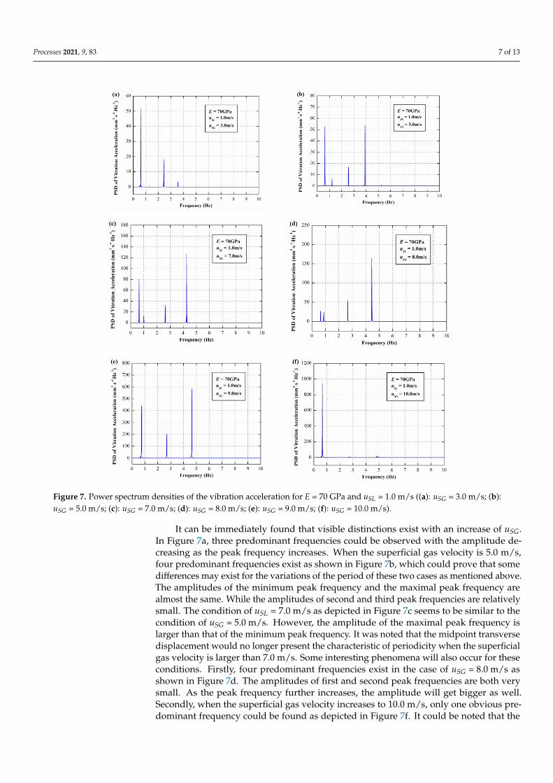
Figure 7. Power spectrum densities of the vibration acceleration for E = 70 GPa and uSL = 1.0 m/s

((a): uSG = 3.0 m/s; (b): uSG = 5.0 m/s; (c): uSG = 7.0 m/s; (d): uSG = 8.0 m/s; (e): uSG = 9.0 m/s; (f): uSG =

10.0 m/s).

It can be immediately found that visible distinctions exist with an increase of uSG. In

Figure 7a, three predominant frequencies could be observed with the amplitude decreas-

ing as the peak frequency increases. When the superficial gas velocity is 5.0 m/s, four pre-

dominant frequencies exist as shown in Figure 7b, which could prove that some differ-

ences may exist for the variations of the period of these two cases as mentioned above.

The amplitudes of the minimum peak frequency and the maximal peak frequency are al-

most the same. While the amplitudes of second and third peak frequencies are relatively

small. The condition of uSL = 7.0 m/s as depicted in Figure 7c seems to be similar to the

condition of uSG = 5.0 m/s. However, the amplitude of the maximal peak frequency is larger

than that of the minimum peak frequency. It was noted that the midpoint transverse dis-

placement would no longer present the characteristic of periodicity when the superficial

gas velocity is larger than 7.0 m/s. Some interesting phenomena will also occur for these

conditions. Firstly, four predominant frequencies exist in the case of uSG = 8.0 m/s as shown

in Figure 7d. The amplitudes of first and second peak frequencies are both very small. As

the peak frequency further increases, the amplitude will get bigger as well. Secondly,

when the superficial gas velocity increases to 10.0 m/s, only one obvious predominant

Figure 7. Power spectrum densities of the vibration acceleration for E = 70 GPa and uSL = 1.0 m/s ((a): uSG = 3.0 m/s; (b):uSG = 5.0 m/s; (c): uSG = 7.0 m/s; (d): uSG = 8.0 m/s; (e): uSG = 9.0 m/s; (f): uSG = 10.0 m/s).

It can be immediately found that visible distinctions exist with an increase of uSG.In Figure 7a, three predominant frequencies could be observed with the amplitude de-creasing as the peak frequency increases. When the superficial gas velocity is 5.0 m/s,four predominant frequencies exist as shown in Figure 7b, which could prove that somedifferences may exist for the variations of the period of these two cases as mentioned above.The amplitudes of the minimum peak frequency and the maximal peak frequency arealmost the same. While the amplitudes of second and third peak frequencies are relativelysmall. The condition of uSL = 7.0 m/s as depicted in Figure 7c seems to be similar to thecondition of uSG = 5.0 m/s. However, the amplitude of the maximal peak frequency islarger than that of the minimum peak frequency. It was noted that the midpoint transversedisplacement would no longer present the characteristic of periodicity when the superficialgas velocity is larger than 7.0 m/s. Some interesting phenomena will also occur for theseconditions. Firstly, four predominant frequencies exist in the case of uSG = 8.0 m/s asshown in Figure 7d. The amplitudes of first and second peak frequencies are both verysmall. As the peak frequency further increases, the amplitude will get bigger as well.Secondly, when the superficial gas velocity increases to 10.0 m/s, only one obvious pre-dominant frequency could be found as depicted in Figure 7f. It could be noted that the

Processes 2021, 9, 83 8 of 13

PSD for the case of uSG = 7.0 m/s and uSG = 9.0 m/s are similar to each other. Merely onemain peak with small amplitude exists in the case of uSG = 7.0 m/s. Then it seems thatconspicuous discrepancies exist in the vibration shapes for these two cases, which meansthat the analysis of PSD of vibration acceleration could really reflect the dynamic responsesof the piping system.

3.2. The Dynamic Responses of E = 120 GPa

The bifurcation diagram of E = 120 GPa is shown in Figure 8. It can be found that thedynamical behavior of uSG = 8.0 m/s seems to be different from other conditions. Yet it ismuch similar to the situation of uSG = 10.0 m/s for E = 70 GPa. In the same way, we willdiscuss the dynamic responses of the piping system of six conditions as shown in Figure 9.

Processes 2021, 9, x FOR PEER REVIEW 8 of 13

frequency could be found as depicted in Figure 7f. It could be noted that the PSD for the

case of uSG = 7.0 m/s and uSG = 9.0 m/s are similar to each other. Merely one main peak with

small amplitude exists in the case of uSG = 7.0 m/s. Then it seems that conspicuous discrep-

ancies exist in the vibration shapes for these two cases, which means that the analysis of

PSD of vibration acceleration could really reflect the dynamic responses of the piping sys-

tem.

3.2. The Dynamic Responses of E = 120 GPa

The bifurcation diagram of E = 120 GPa is shown in Figure 8. It can be found that the

dynamical behavior of uSG = 8.0 m/s seems to be different from other conditions. Yet it is

much similar to the situation of uSG = 10.0 m/s for E = 70 GPa. In the same way, we will

discuss the dynamic responses of the piping system of six conditions as shown in Figure

9.

Figure 8. Bifurcation diagram for the midpoint of the piping system for E = 120 GPa.

Figure 8. Bifurcation diagram for the midpoint of the piping system for E = 120 GPa.

Processes 2021, 9, x FOR PEER REVIEW 8 of 13

frequency could be found as depicted in Figure 7f. It could be noted that the PSD for the

case of uSG = 7.0 m/s and uSG = 9.0 m/s are similar to each other. Merely one main peak with

small amplitude exists in the case of uSG = 7.0 m/s. Then it seems that conspicuous discrep-

ancies exist in the vibration shapes for these two cases, which means that the analysis of

PSD of vibration acceleration could really reflect the dynamic responses of the piping sys-

tem.

3.2. The Dynamic Responses of E = 120 GPa

The bifurcation diagram of E = 120 GPa is shown in Figure 8. It can be found that the

dynamical behavior of uSG = 8.0 m/s seems to be different from other conditions. Yet it is

much similar to the situation of uSG = 10.0 m/s for E = 70 GPa. In the same way, we will

discuss the dynamic responses of the piping system of six conditions as shown in Figure

9.

Figure 8. Bifurcation diagram for the midpoint of the piping system for E = 120 GPa.

Figure 9. Cont.

Processes 2021, 9, 83 9 of 13Processes 2021, 9, x FOR PEER REVIEW 9 of 13

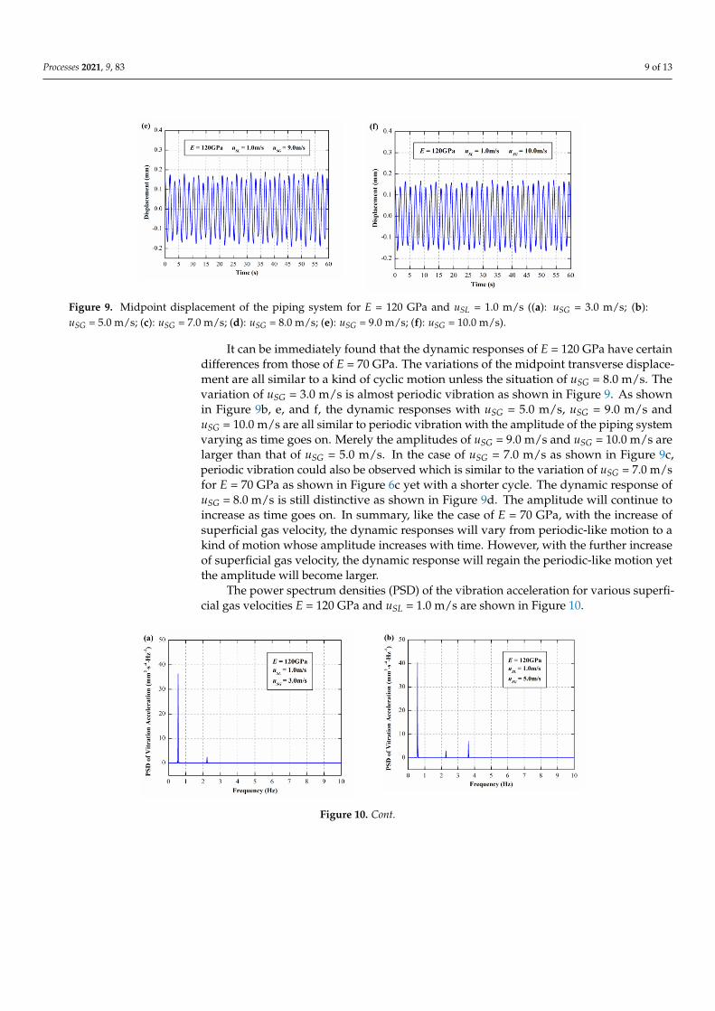
Figure 9. Midpoint displacement of the piping system for E = 120 GPa and uSL = 1.0 m/s ((a): uSG =

3.0 m/s; (b): uSG = 5.0 m/s; (c): uSG = 7.0 m/s; (d): uSG = 8.0 m/s; (e): uSG = 9.0 m/s; (f): uSG = 10.0 m/s).

It can be immediately found that the dynamic responses of E = 120 GPa have certain

differences from those of E = 70 GPa. The variations of the midpoint transverse displace-

ment are all similar to a kind of cyclic motion unless the situation of uSG = 8.0 m/s. The

variation of uSG = 3.0 m/s is almost periodic vibration as shown in Figure 9. As shown in

Figure 9b, e, and f, the dynamic responses with uSG = 5.0 m/s, uSG = 9.0 m/s and uSG = 10.0

m/s are all similar to periodic vibration with the amplitude of the piping system varying

as time goes on. Merely the amplitudes of uSG = 9.0 m/s and uSG = 10.0 m/s are larger than

that of uSG = 5.0 m/s. In the case of uSG = 7.0 m/s as shown in Figure 9c, periodic vibration

could also be observed which is similar to the variation of uSG = 7.0 m/s for E = 70 GPa as

shown in Figure 6c yet with a shorter cycle. The dynamic response of uSG = 8.0 m/s is still

distinctive as shown in Figure 9d. The amplitude will continue to increase as time goes

on. In summary, like the case of E = 70 GPa, with the increase of superficial gas velocity,

the dynamic responses will vary from periodic-like motion to a kind of motion whose

amplitude increases with time. However, with the further increase of superficial gas ve-

locity, the dynamic response will regain the periodic-like motion yet the amplitude will

become larger.

The power spectrum densities (PSD) of the vibration acceleration for various super-

ficial gas velocities E = 120 GPa and uSL = 1.0 m/s are shown in Figure 10.

Figure 9. Midpoint displacement of the piping system for E = 120 GPa and uSL = 1.0 m/s ((a): uSG = 3.0 m/s; (b):uSG = 5.0 m/s; (c): uSG = 7.0 m/s; (d): uSG = 8.0 m/s; (e): uSG = 9.0 m/s; (f): uSG = 10.0 m/s).

It can be immediately found that the dynamic responses of E = 120 GPa have certaindifferences from those of E = 70 GPa. The variations of the midpoint transverse displace-ment are all similar to a kind of cyclic motion unless the situation of uSG = 8.0 m/s. Thevariation of uSG = 3.0 m/s is almost periodic vibration as shown in Figure 9. As shownin Figure 9b, e, and f, the dynamic responses with uSG = 5.0 m/s, uSG = 9.0 m/s anduSG = 10.0 m/s are all similar to periodic vibration with the amplitude of the piping systemvarying as time goes on. Merely the amplitudes of uSG = 9.0 m/s and uSG = 10.0 m/s arelarger than that of uSG = 5.0 m/s. In the case of uSG = 7.0 m/s as shown in Figure 9c,periodic vibration could also be observed which is similar to the variation of uSG = 7.0 m/sfor E = 70 GPa as shown in Figure 6c yet with a shorter cycle. The dynamic response ofuSG = 8.0 m/s is still distinctive as shown in Figure 9d. The amplitude will continue toincrease as time goes on. In summary, like the case of E = 70 GPa, with the increase ofsuperficial gas velocity, the dynamic responses will vary from periodic-like motion to akind of motion whose amplitude increases with time. However, with the further increaseof superficial gas velocity, the dynamic response will regain the periodic-like motion yetthe amplitude will become larger.

The power spectrum densities (PSD) of the vibration acceleration for various superfi-cial gas velocities E = 120 GPa and uSL = 1.0 m/s are shown in Figure 10.

Processes 2021, 9, x FOR PEER REVIEW 9 of 13

Figure 9. Midpoint displacement of the piping system for E = 120 GPa and uSL = 1.0 m/s ((a): uSG =

3.0 m/s; (b): uSG = 5.0 m/s; (c): uSG = 7.0 m/s; (d): uSG = 8.0 m/s; (e): uSG = 9.0 m/s; (f): uSG = 10.0 m/s).

It can be immediately found that the dynamic responses of E = 120 GPa have certain

differences from those of E = 70 GPa. The variations of the midpoint transverse displace-

ment are all similar to a kind of cyclic motion unless the situation of uSG = 8.0 m/s. The

variation of uSG = 3.0 m/s is almost periodic vibration as shown in Figure 9. As shown in

Figure 9b, e, and f, the dynamic responses with uSG = 5.0 m/s, uSG = 9.0 m/s and uSG = 10.0

m/s are all similar to periodic vibration with the amplitude of the piping system varying

as time goes on. Merely the amplitudes of uSG = 9.0 m/s and uSG = 10.0 m/s are larger than

that of uSG = 5.0 m/s. In the case of uSG = 7.0 m/s as shown in Figure 9c, periodic vibration

could also be observed which is similar to the variation of uSG = 7.0 m/s for E = 70 GPa as

shown in Figure 6c yet with a shorter cycle. The dynamic response of uSG = 8.0 m/s is still

distinctive as shown in Figure 9d. The amplitude will continue to increase as time goes

on. In summary, like the case of E = 70 GPa, with the increase of superficial gas velocity,

the dynamic responses will vary from periodic-like motion to a kind of motion whose

amplitude increases with time. However, with the further increase of superficial gas ve-

locity, the dynamic response will regain the periodic-like motion yet the amplitude will

become larger.

The power spectrum densities (PSD) of the vibration acceleration for various super-

ficial gas velocities E = 120 GPa and uSL = 1.0 m/s are shown in Figure 10.

Figure 10. Cont.

Processes 2021, 9, 83 10 of 13Processes 2021, 9, x FOR PEER REVIEW 10 of 13

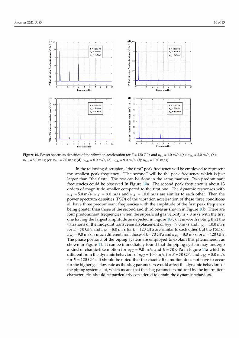
Figure 10. Power spectrum densities of the vibration acceleration for E = 120 GPa and uSL = 1.0 m/s

((a): uSG = 3.0 m/s; (b): uSG = 5.0 m/s; (c): uSG = 7.0 m/s; (d): uSG = 8.0 m/s; (e): uSG = 9.0 m/s; (f): uSG =

10.0 m/s).

In the following discussion, “the first” peak frequency will be employed to represent

the smallest peak frequency. “The second” will be the peak frequency which is just larger

than “the first”. The rest can be done in the same manner. Two predominant frequencies

could be observed In Figure 10a. The second peak frequency is about 13 orders of magni-

tude smaller compared to the first one. The dynamic responses with uSG = 5.0 m/s, uSG =

9.0 m/s and uSG = 10.0 m/s are similar to each other. Then the power spectrum densities

(PSD) of the vibration acceleration of these three conditions all have three predominant

frequencies with the amplitude of the first peak frequency being greater than those of the

second and third ones as shown in Figure 10b. There are four predominant frequencies

when the superficial gas velocity is 7.0 m/s with the first one having the largest amplitude

as depicted in Figure 10(c). It is worth noting that the variations of the midpoint transverse

displacement of uSG = 9.0 m/s and uSG = 10.0 m/s for E = 70 GPa and uSG = 8.0 m/s for E =

120 GPa are similar to each other, but the PSD of uSG = 9.0 m/s is much different from those

of E = 70 GPa and uSG = 8.0 m/s for E = 120 GPa. The phase portraits of the piping system

are employed to explain this phenomenon as shown in Figure 11. It can be immediately

found that the piping system may undergo a kind of chaotic-like motion for uSG = 9.0 m/s

and E = 70 GPa in Figure 11a which is different from the dynamic behaviors of uSG = 10.0

m/s for E = 70 GPa and uSG = 8.0 m/s for E = 120 GPa. It should be noted that the chaotic-

like motion does not have to occur for the higher gas flow rate as the slug parameters

would affect the dynamic behaviors of the piping system a lot, which means that the slug

parameters induced by the intermittent characteristics should be particularly considered

to obtain the dynamic behaviors.

Figure 10. Power spectrum densities of the vibration acceleration for E = 120 GPa and uSL = 1.0 m/s ((a): uSG = 3.0 m/s; (b):uSG = 5.0 m/s; (c): uSG = 7.0 m/s; (d): uSG = 8.0 m/s; (e): uSG = 9.0 m/s; (f): uSG = 10.0 m/s).

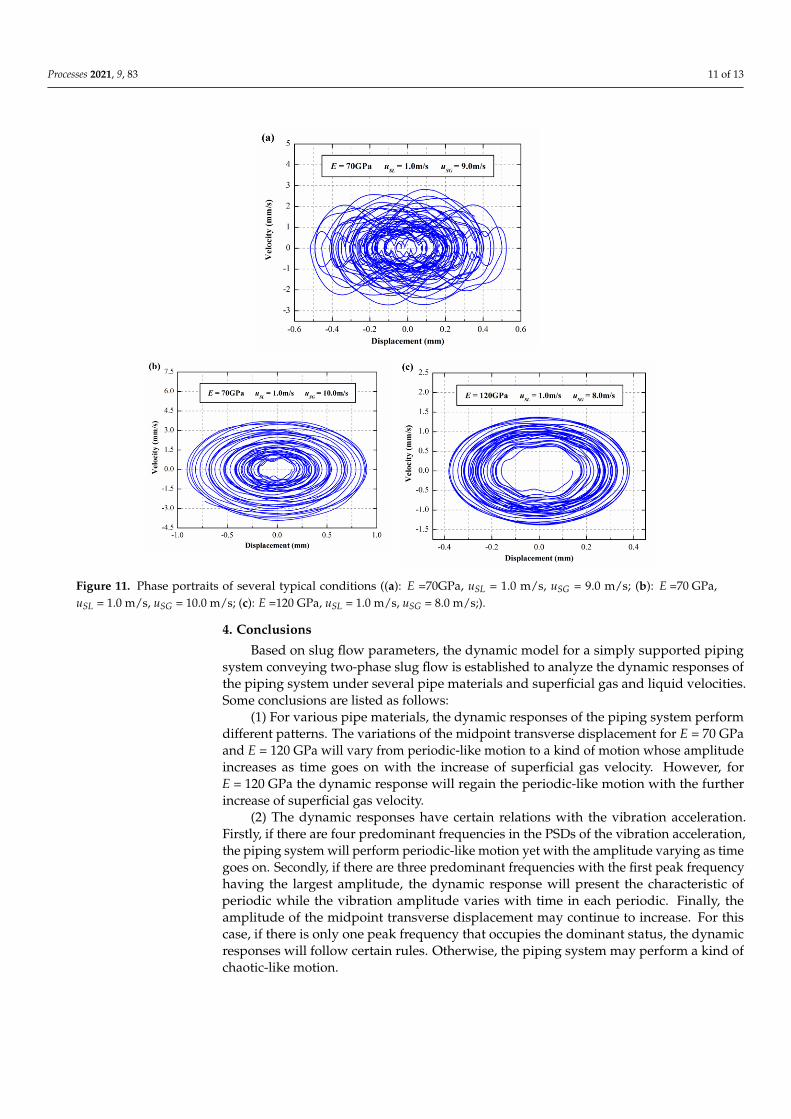
In the following discussion, “the first” peak frequency will be employed to representthe smallest peak frequency. “The second” will be the peak frequency which is justlarger than “the first”. The rest can be done in the same manner. Two predominantfrequencies could be observed In Figure 10a. The second peak frequency is about 13orders of magnitude smaller compared to the first one. The dynamic responses withuSG = 5.0 m/s, uSG = 9.0 m/s and uSG = 10.0 m/s are similar to each other. Then thepower spectrum densities (PSD) of the vibration acceleration of these three conditionsall have three predominant frequencies with the amplitude of the first peak frequencybeing greater than those of the second and third ones as shown in Figure 10b. There arefour predominant frequencies when the superficial gas velocity is 7.0 m/s with the firstone having the largest amplitude as depicted in Figure 10(c). It is worth noting that thevariations of the midpoint transverse displacement of uSG = 9.0 m/s and uSG = 10.0 m/sfor E = 70 GPa and uSG = 8.0 m/s for E = 120 GPa are similar to each other, but the PSD ofuSG = 9.0 m/s is much different from those of E = 70 GPa and uSG = 8.0 m/s for E = 120 GPa.The phase portraits of the piping system are employed to explain this phenomenon asshown in Figure 11. It can be immediately found that the piping system may undergoa kind of chaotic-like motion for uSG = 9.0 m/s and E = 70 GPa in Figure 11a which isdifferent from the dynamic behaviors of uSG = 10.0 m/s for E = 70 GPa and uSG = 8.0 m/sfor E = 120 GPa. It should be noted that the chaotic-like motion does not have to occurfor the higher gas flow rate as the slug parameters would affect the dynamic behaviors ofthe piping system a lot, which means that the slug parameters induced by the intermittentcharacteristics should be particularly considered to obtain the dynamic behaviors.

Processes 2021, 9, 83 11 of 13Processes 2021, 9, x FOR PEER REVIEW 11 of 13

Figure 11. Phase portraits of several typical conditions ((a): E =70GPa, uSL = 1.0 m/s, uSG = 9.0 m/s;

(b): E =70GPa, uSL = 1.0 m/s, uSG = 10.0 m/s; (c): E =120GPa, uSL = 1.0 m/s, uSG = 8.0 m/s;).

4. Conclusions

Based on slug flow parameters, the dynamic model for a simply supported piping

system conveying two-phase slug flow is established to analyze the dynamic responses of

the piping system under several pipe materials and superficial gas and liquid velocities.

Some conclusions are listed as follows:

(1) For various pipe materials, the dynamic responses of the piping system perform

different patterns. The variations of the midpoint transverse displacement for E = 70 GPa

and E = 120 GPa will vary from periodic-like motion to a kind of motion whose amplitude

increases as time goes on with the increase of superficial gas velocity. However, for E =

120 GPa the dynamic response will regain the periodic-like motion with the further in-

crease of superficial gas velocity.

(2) The dynamic responses have certain relations with the vibration acceleration.

Firstly, if there are four predominant frequencies in the PSDs of the vibration acceleration,

the piping system will perform periodic-like motion yet with the amplitude varying as

time goes on. Secondly, if there are three predominant frequencies with the first peak fre-

quency having the largest amplitude, the dynamic response will present the characteristic

of periodic while the vibration amplitude varies with time in each periodic. Finally, the

amplitude of the midpoint transverse displacement may continue to increase. For this

case, if there is only one peak frequency that occupies the dominant status, the dynamic

responses will follow certain rules. Otherwise, the piping system may perform a kind of

chaotic-like motion.

Author Contributions: Conceptualization, Z.H. and Y.W.; methodology, G.L.; software, G.L.; vali-

dation, W.R.; formal analysis, G.L.; investigation, G.L. and W.R; resources, G.L.; data curation,

Figure 11. Phase portraits of several typical conditions ((a): E =70GPa, uSL = 1.0 m/s, uSG = 9.0 m/s; (b): E =70 GPa,uSL = 1.0 m/s, uSG = 10.0 m/s; (c): E =120 GPa, uSL = 1.0 m/s, uSG = 8.0 m/s;).

4. Conclusions

Based on slug flow parameters, the dynamic model for a simply supported pipingsystem conveying two-phase slug flow is established to analyze the dynamic responses ofthe piping system under several pipe materials and superficial gas and liquid velocities.Some conclusions are listed as follows:

(1) For various pipe materials, the dynamic responses of the piping system performdifferent patterns. The variations of the midpoint transverse displacement for E = 70 GPaand E = 120 GPa will vary from periodic-like motion to a kind of motion whose amplitudeincreases as time goes on with the increase of superficial gas velocity. However, forE = 120 GPa the dynamic response will regain the periodic-like motion with the furtherincrease of superficial gas velocity.

(2) The dynamic responses have certain relations with the vibration acceleration.Firstly, if there are four predominant frequencies in the PSDs of the vibration acceleration,the piping system will perform periodic-like motion yet with the amplitude varying as timegoes on. Secondly, if there are three predominant frequencies with the first peak frequencyhaving the largest amplitude, the dynamic response will present the characteristic ofperiodic while the vibration amplitude varies with time in each periodic. Finally, theamplitude of the midpoint transverse displacement may continue to increase. For thiscase, if there is only one peak frequency that occupies the dominant status, the dynamicresponses will follow certain rules. Otherwise, the piping system may perform a kind ofchaotic-like motion.

Processes 2021, 9, 83 12 of 13

Author Contributions: Conceptualization, Z.H. and Y.W.; methodology, G.L.; software, G.L.; vali-dation, W.R.; formal analysis, G.L.; investigation, G.L. and W.R; resources, G.L.; data curation, G.L.;writing—original draft preparation, G.L.; writing—review and editing, Z.H.; visualization, Y.W.;supervision, Z.H.; project administration, Y.W.; funding acquisition, G.L. and Z.H. All authors haveread and agreed to the published version of the manuscript.

Funding: This research was funded by the National Key Research and Development Program ofChina (grant number SQ2019YFC140019-03), the Shandong Key Research and Development Program(grant number 2019JZZY010819), project ZR2020QE192 supported by the Shandong ProvincialNatural, Shandong Key Research and Development Program (grant number 2019GGX104042), andthe Science and Technology Project of Qilu University of Technology (Shandong Academy of Sciences)(grant number 2020QN0024).

Institutional Review Board Statement: Not applicable.

Informed Consent Statement: Not applicable.

Data Availability Statement: Data is contained within the article.

Acknowledgments: The authors would like to thank the editors and reviewers for their valuableand constructive comments.

Conflicts of Interest: The authors declare no conflict of interest.

NomenclatureAi sectional area of the inner pipe, m2

E Young’s modulus of the pipe, GPaI inertial moment of cross-section area, m4

L length of the pipe, mmL(x,t) mass of liquid phase per unit length at the coordinate x and moment t, kg/mmG(x,t) mass of gas phase per unit length at the coordinate x and moment t, kg/mmP mass of fluid per unit length, kg/mQG volume flow rates of the gas, m3/sQL, volume flow rates of the liquid, m3/suL(x,t) local velocity of liquid phase at the coordinate x and moment t, m/suG(x,t) local velocity of gas phase at the coordinate x and moment t, m/suSG superficial gas velocity, m/suSL superficial liquid velocity, m/sy transverse displacement of the pipe, mGreeksymbolsρ density, kg/m3

SubscriptsL liquid phaseG gas phase

References1. Païdoussis, M.; Issid, N. Dynamic stability of pipes conveying fluid. J. Sound Vib. 1974, 33, 267–294. [CrossRef]2. Ariaratnam, S.; Namachchivaya, N.S. Dynamic stability of pipes conveying pulsating fluid. J. Sound Vib. 1986, 107, 215–230.

[CrossRef]3. Jin, J.; Song, Z. Parametric resonances of supported pipes conveying pulsating fluid. J. Fluids Struct. 2005, 20, 763–783. [CrossRef]4. Miwa, S.; Mori, M.; Hibiki, T. Two-phase flow induced vibration in piping systems. Prog. Nucl. Energy 2015, 78, 270–284.

[CrossRef]5. Alamian, R.; Behbahani-Nejad, M.; Ghanbarzadeh, A. A state space model for transient flow simulation in natural gas pipelines.

J. Nat. Gas Sci. Eng. 2012, 9, 51–59. [CrossRef]6. Goodarzi, M.; Safaei, M.R.; Vafai, K.; Ahmadi, G.; Dahari, M.; Kazi, S.; Jomhari, N. Investigation of nanofluid mixed convection in

a shallow cavity using a two-phase mixture model. Int. J. Therm. Sci. 2014, 75, 204–220. [CrossRef]7. Safaei, M.R.; Mahian, O.; Garoosi, F.; Hooman, K.; Karimipour, A.; Kazi, S.N.; Gharehkhani, S. Investigation of Micro- and

Nanosized Particle Erosion in a 90◦ Pipe Bend Using a Two-Phase Discrete Phase Model. Sci. World J. 2014, 2014, 1–12. [CrossRef]8. Pourfattah, F.; Arani, A.A.A.; Babaie, M.R.; Nguyen, H.M.; Asadi, A. On the thermal characteristics of a manifold microchannel

heat sink subjected to nanofluid using two-phase flow simulation. Int. J. Heat Mass Transf. 2019, 143, 118518. [CrossRef]

Processes 2021, 9, 83 13 of 13

9. Almasi, F.; Shadloo, M.; Hadjadj, A.; Ozbulut, M.; Tofighi, N.; Yildiz, M. Numerical simulations of multi-phase electro-hydrodynamics flows using a simple incompressible smoothed particle hydrodynamics method. Comput. Math. Appl. 2021, 81,772–785. [CrossRef]

10. Shadloo, M.; Rahmat, A.; Karimipour, A.; Wongwises, S. Estimation of Pressure Drop of Two-Phase Flow in Horizontal LongPipes Using Artificial Neural Networks. J. Energy Resour. Technol. 2020, 142, 1–21. [CrossRef]

11. Cheng, L.; Ribatski, G.; Thome, J.R. Two-Phase Flow Patterns and Flow-Pattern Maps: Fundamentals and Applications. Appl.Mech. Rev. 2008, 61, 050802. [CrossRef]

12. Al-Safran, E. Investigation and prediction of slug frequency in gas/liquid horizontal pipe flow. J. Pet. Sci. Eng. 2009, 69, 143–155.[CrossRef]

13. Dukler, A.E.; Hubbard, M.G. A Model for Gas-Liquid Slug Flow in Horizontal and Near Horizontal Tubes. Ind. Eng. Chem.Fundam. 1975, 14, 337–347. [CrossRef]

14. Zhang, H.-Q.; Wang, Q.; Sarica, C.; Brill, J.P. Unified model for gas-liquid pipe flow via slug dynamics-part 1: Model development.Trans. ASME J. Energy Resour. Technol. 2003, 125, 266–273. [CrossRef]

15. Riverin, J.; De Langre, E.; Pettigrew, M.J. Fluctuating forces caused by internal two-phase flow on bends and tees. J. Sound Vib.2006, 298, 1088–1098. [CrossRef]

16. Cargnelutti, M.F.; Belfroid, S.P.C.; Schiferli, W. Two-Phase Flow-Induced Forces on Bends in Small Scale Tubes. J. Press. Vessel.Technol. 2010, 132, 041305. [CrossRef]

17. Liu, Y.; Miwa, S.; Hibiki, T.; Ishii, M.; Morita, H.; Kondoh, Y.; Tanimoto, K. Experimental study of internal two-phase flow inducedfluctuating force on a 90◦ elbow. Chem. Eng. Sci. 2012, 76, 173–187. [CrossRef]

18. Giraudeau, M.; Mureithi, N.W.; Pettigrew, M.J. Two-Phase Flow-Induced Forces on Piping in Vertical Upward Flow: ExcitationMechanisms and Correlation Models. J. Press. Vessel. Technol. 2013, 135, 030907. [CrossRef]

19. An, C.; Su, J. Vibration Behavior of Marine Risers Conveying Gas-Liquid Two-Phase Flow. In Proceedings of the Volume 9: OceanRenewable Energy; ASME International: New York, NY, USA, 2015.

20. Ebrahimi-Mamaghani, A.; Sotudeh-Gharebagh, R.; Zarghami, R.; Mostoufi, N. Dynamics of two-phase flow in vertical pipes. J.Fluids Struct. 2019, 87, 150–173. [CrossRef]

21. Sazesh, S.; Shams, S. Vibration analysis of cantilever pipe conveying fluid under distributed random excitation. J. Fluids Struct.2019, 87, 84–101. [CrossRef]

22. Khudayarov, B.; Komilova, K.; Turaev, F. Numerical Modeling of pipes conveying gas-liquid two-phase flow. In Proceedings ofthe E3S Web of Conferences; EDP Sciences: Les Ulis, France, 2019; Volume 97, p. 05022.

23. Zhu, H.; Zhao, H.-L.; Gao, Y. Experimental Investigation of Vibration Response of a Free-Hanging Flexible Riser Induced byInternal Gas-Liquid Slug Flow. China Ocean Eng. 2018, 32, 633–645. [CrossRef]

24. Cabrera-Miranda, J.M.; Paik, J.K. Two-phase flow induced vibrations in a marine riser conveying a fluid with rectangular pulsetrain mass. Ocean Eng. 2019, 174, 71–83. [CrossRef]

25. Wang, L. A further study on the non-linear dynamics of simply supported pipes conveying pulsating fluid. Int. J. Non-LinearMech. 2009, 44, 115–121. [CrossRef]

26. Liu, G.; Wang, Y. Natural frequency analysis of a cantilevered piping system conveying gas–liquid two-phase slug flow. Chem.Eng. Res. Des. 2018, 136, 564–580. [CrossRef]

27. Zhang, H.Q.; Wang, Q.; Sarica, C.; Brill, J.P. Unified model for gas-liquid pipe flow via slug dynamics-part 2: Model validation.Trans. ASME J. Energy Resour. Technol. 2003, 125, 274–283. [CrossRef]