Honor Code Statement

“We affirm that we have carried out all of our academic endeavors with full academic

honesty.”

Signed,

Harrison Bourikas (Electronically Signed) Patrick DeBenedetto (Electronically Signed)

TO: Ann Anderson, Professor

FROM: Patrick DeBenedetto and Harrison Bourikas, Students P.D., H.B.

DATE: March 1, 2013

SUBJECT: Surface Pressure Testing – Baja Pickup Truck

Opening: The purpose of this correspondence is to report on our findings about the variations in

surface pressure and pressure coefficient at a series of locations along the body of a 1:12 model Baja

pickup truck for two different wind tunnel motor frequencies in an Aerovent 22- 560 BIA CB 2184-10

Model 402 CB Wind Tunnel.

Experimental Results: The surface pressures for each of the 12 taps on the model are shown in

Figure 1, and the respective calculated pressure coefficients are shown in Figure 2.

Figure 1.

Figure 2 is a plot of the surface pressures at each of the twelve pressure taps (complete with uncertainties) against

the position of the tap. Note that the car is upside-down to better illustrate how surface pressure decreases as the

flow moves over a shoulder on the body, and vice versa.

Figure 2.

Figure 2 is a plot of the pressure coefficients at each of the twelve pressure taps (complete with uncertainties) against

the position of the tap. Note that the car is upside-down to better illustrate how the pressure coefficient decreases as

the flow moves over a shoulder on the body, and vice versa.

Simultaneous examination of Figures 1 and 2 shows that the pressure coefficient increases as the

surface pressure increases locations up to 120 mm for both motor frequencies. Thus, for these taps,

-700

-600

-500

-400

-300

-200

-100

0

100

200

300

0 50 100 150 200 250

Pre

ssu

re (

Pa)

Pressure Port Location (mm)

20 Hz

40 Hz

-1.0

-0.5

0.0

0.5

1.0

1.5

2.0

0 50 100 150 200 250

Pre

ssu

re C

oef

fici

ent

Pressure Port Location (mm)

20 Hz

40 Hz

Euler’s Equation holds, and we may infer that the flow is laminar. For locations farther than 120 mm,

particularly for the 40 Hz tests, this relationship is not as evident. Thus, Euler’s Equation does not

hold and we may infer that the flow is turbulent, just as we would expect.

Experimental Setup & Procedure: A 1:12 scale model of a Baja pickup truck complete with twelve

pressure taps was placed on the dynamometer in the wind tunnel. In addition, a pitot probe was placed

in the tunnel some distance from the model to gather data about the wind flow in the tunnel. The pitot

probe and each of the 12 taps were connected to an input channel on the pressure transducer using

Tygon tubes. One-hundred voltage readings were taken for each of the twelve pressure taps and the

pitot probe. The data was analyzed, and the velocity of the wind in the tunnel and the free stream static

pressure were calculated using the data acquired from the pitot probe. Once these values had been

determined, the surface pressure and pressure coefficient were calculated for each of the taps and the

pitot probe. These values were then plotted against the location of each tap to determine how each

value varied over the body of the model. In addition, the uncertainties associated with the surface

pressure and pressure coefficient were calculated in order to determine the accuracy and usefulness of

the data.

Discussion & Closing: Our data clearly shows that there is a great deal of variation in the surface

pressure and pressure coefficient over the body of the model Baja pickup truck. The values for the

pressure coefficient and surface pressure in the 20 Hz testing seem to follow some sort of pattern up

until tap 7 (the top of the pickup cab). After tap 7, the data is much more erratic. This indicates that

the flow over the model is laminar up until tap 7, at which point the flow appears to have separated and

become turbulent. The data from the 40 Hz tests follows this same general pattern, it does show a

greater variation from point to point; that is, the pattern followed by the data up until tap 7 is not as

easily discernible as it is for the 20 Hz tests. This is primarily due to the fact that flows behave more

turbulently at higher velocities. For both tests, the flow appears to be laminar up until tap 7; thus,

Euler’s Equation applies, and we can see that for both the 20 and 40 Hz tests the pressure coefficient

increases as the surface pressure decreases, and vice versa. I would recommend adding more pressure

taps to the model, as this would allow for the collection of more data with which to examine the flow

over the model. In addition, I would also recommend further testing for taps 8-12 to better determine

the characteristics of the turbulent flow over these taps.

If we could be of any further assistance in clarifying any of the information presented or in moving

ahead with further testing and analysis, please do not hesitate to contact us.

Contact Information:

Patrick DeBenedetto, Student, Union College Harrison Bourikas, Student, Union College

Cell Phone: 1-978-821-1081 Cell Phone: 1-781-974-5108

Email: debenedp@garnet.union.edu Email: bourikah@garnet.union.edu

List of Appendixes:

A. Summary Table of all data

B. Surface pressure data, calculations & plot, velocity calculations

C. Pressure coefficient calculations, table of values, and plot

D. Uncertainty calculations for velocity, surface pressure, and pressure coefficient

E. Experimental setup & procedure

F. Model specs & pressure tap locations

G. Configuring InstaCal and Tracer DAQ Pro for data collection

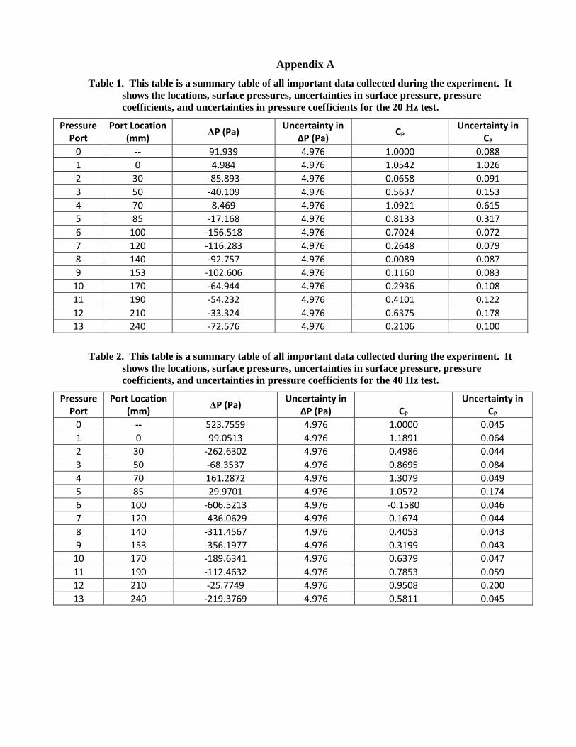
Appendix A

Table 1. This table is a summary table of all important data collected during the experiment. It

shows the locations, surface pressures, uncertainties in surface pressure, pressure

coefficients, and uncertainties in pressure coefficients for the 20 Hz test.

Pressure Port

Port Location (mm)

ΔP (Pa) Uncertainty in

ΔP (Pa) CP

Uncertainty in CP

0 -- 91.939 4.976 1.0000 0.088

1 0 4.984 4.976 1.0542 1.026

2 30 -85.893 4.976 0.0658 0.091

3 50 -40.109 4.976 0.5637 0.153

4 70 8.469 4.976 1.0921 0.615

5 85 -17.168 4.976 0.8133 0.317

6 100 -156.518 4.976 0.7024 0.072

7 120 -116.283 4.976 0.2648 0.079

8 140 -92.757 4.976 0.0089 0.087

9 153 -102.606 4.976 0.1160 0.083

10 170 -64.944 4.976 0.2936 0.108

11 190 -54.232 4.976 0.4101 0.122

12 210 -33.324 4.976 0.6375 0.178

13 240 -72.576 4.976 0.2106 0.100

Table 2. This table is a summary table of all important data collected during the experiment. It

shows the locations, surface pressures, uncertainties in surface pressure, pressure

coefficients, and uncertainties in pressure coefficients for the 40 Hz test.

Pressure Port

Port Location (mm)

ΔP (Pa) Uncertainty in

ΔP (Pa) CP Uncertainty in

CP

0 -- 523.7559 4.976 1.0000 0.045

1 0 99.0513 4.976 1.1891 0.064

2 30 -262.6302 4.976 0.4986 0.044

3 50 -68.3537 4.976 0.8695 0.084

4 70 161.2872 4.976 1.3079 0.049

5 85 29.9701 4.976 1.0572 0.174

6 100 -606.5213 4.976 -0.1580 0.046

7 120 -436.0629 4.976 0.1674 0.044

8 140 -311.4567 4.976 0.4053 0.043

9 153 -356.1977 4.976 0.3199 0.043

10 170 -189.6341 4.976 0.6379 0.047

11 190 -112.4632 4.976 0.7853 0.059

12 210 -25.7749 4.976 0.9508 0.200

13 240 -219.3769 4.976 0.5811 0.045

Appendix B

Table 3. This table shows the locations, average voltage readings, pressures, and percent

standard deviations for each of the pressure taps on the model during the 20 Hz

surface pressure test.

Pressure Port

Port Location (mm)

Average Voltage Reading (V)

ΔP (Pa) % Standard Deviation in

ΔP

0 -- 0.2231 91.939 1.2673

1 0 0.0435 4.984 6.9341

2 30 -0.1441 -85.893 0.7106

3 50 -0.0496 -40.109 6.9546

4 70 0.0507 8.469 5.7325

5 85 -0.0022 -17.168 1.6360

6 100 -0.2900 -156.518 0.7315

7 120 -0.2069 -116.283 0.7529

8 140 -0.1583 -92.757 1.1457

9 153 -0.1787 -102.606 0.7581

10 170 -0.1009 -64.944 0.7862

11 190 -0.0788 -54.232 1.8476

12 210 -0.0356 -33.324 2.7783

13 240 -0.1166 -72.576 0.6764

Table 4. This table shows the locations, average voltage readings, pressures, and percent

standard deviations for each of the pressure taps on the model during the 40 Hz

surface pressure test.

Pressure Port

Port Location (mm)

Average Voltage Reading (V)

ΔP (Pa) % Standard Deviation in

ΔP

0 -- 1.1149 523.7559 0.9554

1 0 0.2378 99.0513 1.2520

2 30 -0.5091 -262.6302 1.2797

3 50 -0.1079 -68.3537 7.3887

4 70 0.3663 161.2872 1.6583

5 85 0.0951 29.9701 1.6217

6 100 -1.2193 -606.5213 0.8631

7 120 -0.8673 -436.0629 0.8626

8 140 -0.6100 -311.4567 1.2851

9 153 -0.7024 -356.1977 0.9621

10 170 -0.3584 -189.6341 1.2647

11 190 -0.1990 -112.4632 4.0557

12 210 -0.0200 -25.7749 30.9954

13 240 -0.4198 -219.3769 1.0525

It is important to note that the location of each pressure port in Tables 3 and 4 is relative to the

front of the model. Pressure port 4, for example, is located 70 mm from the front of the model

truck. Also, note that pressure port 0 does not have a location. This is because pressure port 0

corresponds to the pitot probe, which was not located on the model. It was placed far enough

away from the model in the wind tunnel such that flow into the probe was not affected by the

fluctuating flow patterns around the model. During our data acquisition, we discovered that the

pressure transducer had somehow been calibrated to output voltages with the sign opposite of

what it should have been. In order to correct for this, we simply modified our average of the

100 voltage readings for each pressure port by (-1). The average voltage readings presented in

Tables 1 and 2 are these corrected voltages.

In order to calculate the surface pressure, ΔP, for each port, we calculated ΔP for each of the

100 voltage readings for each port. The voltage readings used in this calculation were not the

corrected average voltage readings. In order to calculate ΔP for each reading, we used the

calibration curve for the pressure transducer used in the experiment. This curve is modeled by

the equation:

(1)

Where ΔP is the surface pressure and E is the voltage reading for the pressure port. Once ΔP

had been calculated for each voltage reading, we took the average of all of the calculated

surface pressures and then multiplied this average by -1 to correct for the incorrect sign

calibration of the pressure transducer. The surface pressures reported in Tables 3 and 4 are the

corrected average surface pressures for each port.

The percent standard deviation in the surface pressure was calculated using the following Excel

function:

[ ( )

] (2)

Where ABS is the absolute value function, STDEV.S is the standard deviation function, ΔP1-100

is the population containing the calculated surface pressures for all 100 voltage readings, and

ΔPAVG is the corrected average surface pressure for all 100 voltage readings described above.

For the most part, the percent standard deviations for each pressure port in both the 20 and 40

Hz tests were somewhere around 1%, which is perfectly reasonable. There were several,

however, that were well outside this range. In the 20 Hz test pressure ports 1, 3, and 4 reported

standard deviations of 6.93%, 6.95%, and 5.73%, respectively. In the 40 Hz test, pressure ports

3, 11, and 12 reported standard deviations of 7.39%, 4.06%, and 40.00%, respectively. This

was alarming at first, but when we examined the locations of these ports on the model Baja

pickup, we noticed that they were at locations in which flow was not laminar (as expected), but

turbulent and erratic. Thus, the deviation of the surface pressures at these locations was not out

of the ordinary.

In order to gain a better understanding of the flow over the model Baja pickup, the average

corrected surface pressures (ΔP) were plotted against the pressure port location. The

uncertainty for each of these surface pressures was calculated as ±4.98 Pa for each value.

Figure 3.

Figure 3 is a plot of the surface pressures at each of the twelve pressure taps (complete with uncertainties)

against the position of the tap for both the 20 Hz and 40 Hz tests.

Velocity Calculations

In order to calculate the velocity of the wind in the tunnel far away from the model, data was

gathered using a pitot probe (pressure port 0 in Tables 3 and 4). In addition, the temperature of

the air in the wind tunnel was measured. For both the 20 Hz and 40 Hz tests, this temperature

was 23°C. Prior to calculating the wind velocity, the density of the air in the tunnel was

calculated using the following equation:

(3)

Where ρ is the air density, P is the ambient air pressure, R is the specific gas constant for air,

and T is the air temperature in Kelvin. Substituting our known and measured values into

equation (3), we were able to calculate the density of the air in the tunnel.

(

)( )

Using this calculated density, we applied Bernoulli’s Equation for an incompressible, steady,

inviscid flow along a streamline to calculate the velocity of the air in the tunnel far away from

the model Baja pickup for both the 20 and 40 Hz tests.

√

. (4)

-700.0

-600.0

-500.0

-400.0

-300.0

-200.0

-100.0

0.0

100.0

200.0

300.0

0 50 100 150 200 250

Pre

ssu

re (

Pa)

Pressure Port Location (mm)

20 Hz

40 Hz

Where V is the wind velocity, ΔP is difference between the stagnation and static pressures

(given as ΔP for pressure port 0 in Tables 3 and 4), and ρ is the density of the air in the tunnel.

Substituting for our known and calculated values for the 20 and 40 Hz tests, we could see that:

√ ( )

√ ( )

These values differ from the 16.484 m/s (for a motor frequency of 20 Hz) and 33.592 m/s (for a

motor frequency of 40 Hz) values provided by the manufacturer of the wind tunnel, but it is

important to remember that the manufacturer’s data is more or less a ballpark estimate (albeit a

good one) of what the velocity of the wind in the tunnel should be at a given motor frequency.

Appendix C

Table 4. This table shows the locations, difference between static and free stream surface

pressure, pressure coefficient, and percent uncertainty in the pressure coefficient

for each of the pressure taps on the model during the 20 Hz surface pressure test.

Pressure Port

Port Location (mm)

Ps - Pfree stream static (Pa) CP % Uncertainty in CP

0 -- 91.9391 1.0000 8.76

1 0 96.9228 1.0542 97.29

2 30 6.0462 0.0658 138.13

3 50 51.8304 0.5637 27.14

4 70 100.4082 1.0921 56.30

5 85 74.7707 0.8133 39.03

6 100 64.5791 0.7024 10.26

7 120 24.3437 0.2648 29.76

8 140 0.8181 0.0089 980.34

9 153 10.6668 0.1160 71.61

10 170 26.9955 0.2936 36.63

11 190 37.7072 0.4101 29.69

12 210 58.6147 0.6375 27.89

13 240 19.3631 0.2106 47.58

Table 5. This table shows the locations, difference between static and free stream surface

pressure, pressure coefficient, and percent uncertainty in the pressure coefficient

for each of the pressure taps on the model during the 40 Hz surface pressure test.

Pressure Port

Port Location (mm)

PS - Pfree stream static (Pa) CP % Uncertainty in CP

0 -- 523.7559 1.0000 4.47

1 0 424.7046 1.1891 5.37

2 30 786.3860 0.4986 8.76

3 50 592.1095 0.8695 9.64

4 70 362.4686 1.3079 3.77

5 85 493.7857 1.0572 16.41

6 100 1130.2771 -0.1580 -29.07

7 120 959.8187 0.1674 26.08

8 140 835.2126 0.4053 10.64

9 153 879.9535 0.3199 13.47

10 170 713.3900 0.6379 7.32

11 190 636.2191 0.7853 7.52

12 210 549.5308 0.9508 21.05

13 240 743.1327 0.5811 7.74

It is important to note that the location of each pressure port in Tables 4 and 5 is relative to the

front of the model. Pressure port 4, for example, is located 70 mm from the front of the model

truck. Also, note that pressure port 0 does not have a location. This is because pressure port 0

corresponds to the pitot probe, which was not located on the model. It was placed far enough

away from the model in the wind tunnel such that flow into the probe was not affected by the

fluctuating flow patterns around the model.

In order to calculate the difference between the surface pressure and the static free stream

pressure for both the 20 Hz and 40 Hz at each pressure port, the following relationship was

used:

( ) ( )

Where the “ ” term is the desired pressure difference, the “

” term is the ΔP quantity reported in Tables 4 and 5 for pressure ports 1-13, and the

“ ” term is the ΔP quantity reported in Tables 4 and 5 for port 0

(the pitot probe). Note that the ΔP term for port 0 is not the same for the 20 Hz and 40 Hz tests,

and the appropriate value must be used. For some pressure ports, this sum was a negative

quantity. In order to correct for this, the absolute value function was applied to the right side of

equation (5). Thus, (5) became:

[( ) ( )] (5)

The absolute value needed to be applied because the quantity PS - Pfree stream static was later

appears in the denominator of the equation used to calculate the pressure coefficient for each

pressure port. We know that the pressure coefficient cannot be negative, and the only way to

return a negative value would be to have a negative PS - Pfree stream static term. Thus, the value for

every PS - Pfree stream static must be positive.

With the PS - Pfree stream static value calculated for each pressure port in the 20 and 40 Hz tests, we

had defined all of the variables necessary to calculate the pressure coefficient, CP. This was

accomplished using:

(6)

Where CP is the pressure coefficient, PS - Pfree stream static is the same as defined above, ρ is the density of

the air in the tunnel, and V is the velocity of the wind in the tunnel. For each calculation, ρ remained a

constant at 1.192 kg/m3. For the 20 Hz test, V = V20 Hz = 12.422 m/s, and for the 40 Hz test V = V40 Hz =

26.649 m/s. For an outline of how V20 Hz, V40 Hz, and ρ were calculated, please consult Appendix A.

Substituting ρ and V20 Hz into (6), we were able to generate an equation for the pressure coefficient at

each pressure port in the 20 Hz test:

(7)

Performing this same substitution with ρ and V40 Hz yields an equation for the pressure coefficient at

each pressure port in the 40 Hz test:

(8)

Substituting the results obtained from equation (5) for a particular pressure port in the 20 Hz test into

equation (7) yielded the pressure coefficient, CP, for the pressure port in question. Likewise,

substituting the result from (5) for a particular pressure port in the 40 Hz test into equation (8) yielded

the pressure coefficient for the port in question.

In order to gain a better understanding of the flow over the model Baja pickup, the pressure

coefficients of each port were plotted against the pressure port’s location. The uncertainty for each of

these surface pressures was calculated individually (please consult Appendix D for an outline of how

these uncertainties were calculated).

Figure 4.

Figure 4 is a plot of the pressure coefficients at each of the twelve pressure taps (complete with uncertainties) against

the position of the tap for both the 20 Hz and 40 Hz tests.

-1.0

-0.5

0.0

0.5

1.0

1.5

2.0

0 50 100 150 200 250Pre

ssu

re C

oef

fici

ent

Pressure Probe Location (mm)

20 Hz

40 Hz

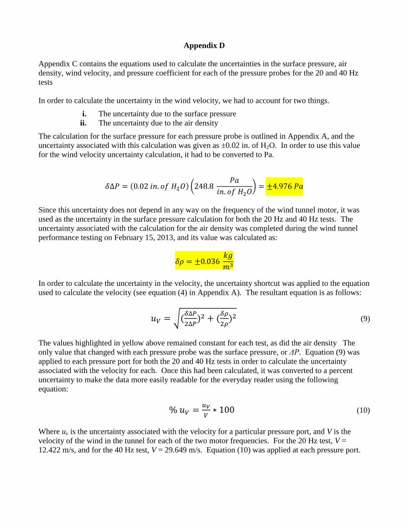
Appendix D

Appendix C contains the equations used to calculate the uncertainties in the surface pressure, air

density, wind velocity, and pressure coefficient for each of the pressure probes for the 20 and 40 Hz

tests

In order to calculate the uncertainty in the wind velocity, we had to account for two things.

i. The uncertainty due to the surface pressure

ii. The uncertainty due to the air density

The calculation for the surface pressure for each pressure probe is outlined in Appendix A, and the

uncertainty associated with this calculation was given as ±0.02 in. of H2O. In order to use this value

for the wind velocity uncertainty calculation, it had to be converted to Pa.

( ) (

)

Since this uncertainty does not depend in any way on the frequency of the wind tunnel motor, it was

used as the uncertainty in the surface pressure calculation for both the 20 Hz and 40 Hz tests. The

uncertainty associated with the calculation for the air density was completed during the wind tunnel

performance testing on February 15, 2013, and its value was calculated as:

In order to calculate the uncertainty in the velocity, the uncertainty shortcut was applied to the equation

used to calculate the velocity (see equation (4) in Appendix A). The resultant equation is as follows:

√(

) (

) (9)

The values highlighted in yellow above remained constant for each test, as did the air density The

only value that changed with each pressure probe was the surface pressure, or ΔP. Equation (9) was

applied to each pressure port for both the 20 and 40 Hz tests in order to calculate the uncertainty

associated with the velocity for each. Once this had been calculated, it was converted to a percent

uncertainty to make the data more easily readable for the everyday reader using the following

equation:

(10)

Where uv is the uncertainty associated with the velocity for a particular pressure port, and V is the

velocity of the wind in the tunnel for each of the two motor frequencies. For the 20 Hz test, V =

12.422 m/s, and for the 40 Hz test, V = 29.649 m/s. Equation (10) was applied at each pressure port.

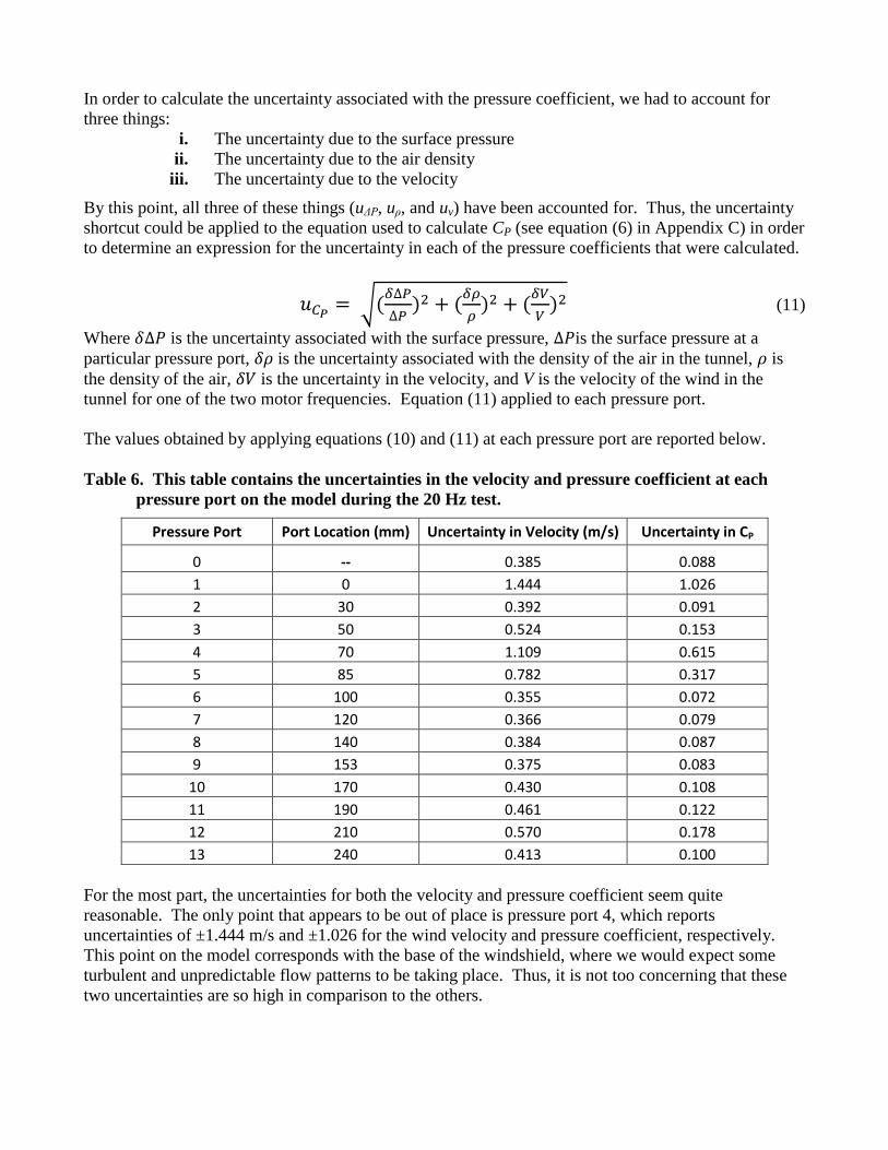
In order to calculate the uncertainty associated with the pressure coefficient, we had to account for

three things:

i. The uncertainty due to the surface pressure

ii. The uncertainty due to the air density

iii. The uncertainty due to the velocity

By this point, all three of these things (uΔP, uρ, and uv) have been accounted for. Thus, the uncertainty

shortcut could be applied to the equation used to calculate CP (see equation (6) in Appendix C) in order

to determine an expression for the uncertainty in each of the pressure coefficients that were calculated.

√(

) (

) (

) (11)

Where is the uncertainty associated with the surface pressure, is the surface pressure at a

particular pressure port, is the uncertainty associated with the density of the air in the tunnel, is

the density of the air, is the uncertainty in the velocity, and V is the velocity of the wind in the

tunnel for one of the two motor frequencies. Equation (11) applied to each pressure port.

The values obtained by applying equations (10) and (11) at each pressure port are reported below.

Table 6. This table contains the uncertainties in the velocity and pressure coefficient at each

pressure port on the model during the 20 Hz test.

Pressure Port Port Location (mm) Uncertainty in Velocity (m/s) Uncertainty in CP

0 -- 0.385 0.088

1 0 1.444 1.026

2 30 0.392 0.091

3 50 0.524 0.153

4 70 1.109 0.615

5 85 0.782 0.317

6 100 0.355 0.072

7 120 0.366 0.079

8 140 0.384 0.087

9 153 0.375 0.083

10 170 0.430 0.108

11 190 0.461 0.122

12 210 0.570 0.178

13 240 0.413 0.100

For the most part, the uncertainties for both the velocity and pressure coefficient seem quite

reasonable. The only point that appears to be out of place is pressure port 4, which reports

uncertainties of ±1.444 m/s and ±1.026 for the wind velocity and pressure coefficient, respectively.

This point on the model corresponds with the base of the windshield, where we would expect some

turbulent and unpredictable flow patterns to be taking place. Thus, it is not too concerning that these

two uncertainties are so high in comparison to the others.

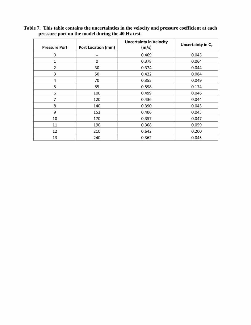
Table 7. This table contains the uncertainties in the velocity and pressure coefficient at each

pressure port on the model during the 40 Hz test.

Pressure Port Port Location (mm) Uncertainty in Velocity

(m/s) Uncertainty in CP

0 -- 0.469 0.045

1 0 0.378 0.064

2 30 0.374 0.044

3 50 0.422 0.084

4 70 0.355 0.049

5 85 0.598 0.174

6 100 0.499 0.046

7 120 0.436 0.044

8 140 0.390 0.043

9 153 0.406 0.043

10 170 0.357 0.047

11 190 0.368 0.059

12 210 0.642 0.200

13 240 0.362 0.045

Appendix E

This appendix contains a schematic diagram of the experimental setup for the surface pressure testing,

as well as a detailed explanation of how the experiment was carried out and how certain calculations

were made.

The experimental setup for testing the surface pressure at a series of locations along the model of the

Baja pickup truck was slightly complex but very user-friendly. In order to complete the experiment,

the following devices were needed:

i. 1:12 model Baja pickup truck complete with 12 pressure taps and Tygon tubes

ii. Pressure transducer with 10 ports (provided by the lab instructor, model and serial number

unknown) and labeled Tygon tubes leading from each

iii. Aerovent 22- 560 BIA CB 2184-10 Model 402 CB Wind Tunnel

iv. Pitot probe

v. Data Acquisition System (DAQ)

vi. InstaCal and Tracer DAQ Pro software

vii. Desktop or laptop computer

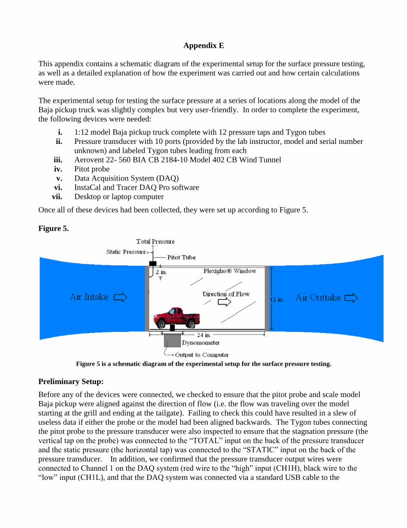
Once all of these devices had been collected, they were set up according to Figure 5.

Figure 5.

Figure 5 is a schematic diagram of the experimental setup for the surface pressure testing.

Preliminary Setup:

Before any of the devices were connected, we checked to ensure that the pitot probe and scale model

Baja pickup were aligned against the direction of flow (i.e. the flow was traveling over the model

starting at the grill and ending at the tailgate). Failing to check this could have resulted in a slew of

useless data if either the probe or the model had been aligned backwards. The Tygon tubes connecting

the pitot probe to the pressure transducer were also inspected to ensure that the stagnation pressure (the

vertical tap on the probe) was connected to the “TOTAL” input on the back of the pressure transducer

and the static pressure (the horizontal tap) was connected to the “STATIC” input on the back of the

pressure transducer. In addition, we confirmed that the pressure transducer output wires were

connected to Channel 1 on the DAQ system (red wire to the “high” input (CH1H), black wire to the

“low” input (CH1L), and that the DAQ system was connected via a standard USB cable to the

computer. Before any data collection began, the temperature of the air in the wind tunnel in degrees

Celsius was recorded. This value, along with the ambient air pressure and the specific gas constant for

air, was used to calculate the density of the air in the wind tunnel (please consult Appendix B for the

full calculation outline).

Initial Round of Testing:

The Tygon tubes leading from pressure taps 1-9 on the scale model Baja were connected to their

corresponding, multicolored tubes leading to the inputs on the back of the pressure transducer. Port 1

was connected to tube 1, port 2 was connected to tube 2, and so on until all of the tubes had been

connected. It is important to note that the pressure transducer only has 10 channels on it. Thus, data

for all of the pressure taps on the model could not be collected at once (this problem is dealt with later

in this appendix). Before proceeding any further, we double checked our tube connections to ensure

that the pressure taps were connected to the proper transducer channels. Failure to do this could result

in incorrect data for certain ports.

With the devices connected, the data acquisition system and software packages (InstaCal and Tracer

DAQ Pro) were configured to collect the data. For a detailed explanation of how to set up the software

packages, please consult Appendix G.

The wind tunnel was then switched on, and the motor frequency was set to 20 Hz. Several minutes

were allowed to pass in order to give the motor, and therefore the air flow in the tunnel, time to

stabilize. During this time, we turned the selector switch on the pressure transducer (the large black

switch on the front of the box) to Channel 0. This channel corresponded to the pitot probe.

Data Collection:

The DAQ was then triggered to begin collecting data. 100 voltage readings were taken for the

pitot probe. After all of the data had been collected, it was saved and then opened in a

Microsoft Excel file for analysis (see Appendix G for instructions on how to perform this

action).

With the data saved, we turned the selector switch on the pressure transducer to Channel 1.

This instructed the transducer to output voltage readings corresponding to the difference in the

local pressure at pressure tap 1 on the model and the static pressure of the flow (read from the

pitot probe). With Channel 1 selected, the data acquisition system was triggered to begin

collecting data, and 100 voltage readings were taken. Once the data had been collected, it was

saved and then opened in a Microsoft Excel file for analysis.

The steps outlined under the “Data Collection” subheading were repeated for Channels 2-9 on the

transducer (corresponding to pressure taps 2-9 on the scale model of the Baja pickup). With all of the

data collected for pressure taps 1-9, the frequency of the wind tunnel motor was increased to 40 Hz.

Once again, the motor, and therefore the air flow in the tunnel, were given several minutes to stabilize.

During this time, we turned the selector switch on the pressure transducer (the large black switch on

the front of the box) back to Channel 0.

When the flow had steadied, we repeated the steps outlined under the “Data Collection” subheading 10

times to collect voltage readings for the pitot probe and the first 9 pressure taps on the scale model for

the new motor frequency of 40 Hz. Once these 10 rounds of data collection had been completed, the

wind tunnel was switched off, and all of the Tygon tubes connecting the pressure taps to the pressure

transducer were disconnected. The Tygon tubes from ports 10-13 were then connected to the

multicolored tubes labeled 1, 2, 3, and 4 (10 connected to 1, 11 connected to 2, and so on) leading to

the inputs on the back of the pressure transducer. The wind tunnel was then switched on, and the

motor frequency was set to 20 Hz. Several minutes were allowed to pass in order to give the motor,

and therefore the air flow in the tunnel, time to stabilize. During this time, we turned the selector

switch on the pressure transducer (the large black switch on the front of the box) to Channel 1. This

channel corresponded to pressure tap 10 on the model. The steps outlined under the “Data Collection”

subheading were then followed and subsequently repeated 3 more times to collect data for pressure

taps 11, 12, and 13 on the scale model.

With all of the data collected for the 20 Hz test, the frequency of the wind tunnel motor was increased

to 40 Hz. Once again, the motor, and therefore the air flow in the tunnel, were given several minutes

to stabilize. During this time, we turned the selector switch on the pressure transducer (the large black

switch on the front of the box) back to Channel 1. When the flow had steadied, we repeated the steps

outlined under the “Data Collection” subheading 4 more times to collect voltage readings for the last 4

taps on the scale model for the new motor frequency of 40 Hz. Once these steps had been completed,

the wind tunnel motor was switched off for good.

Data Analysis:

The standard deviation and the percent standard deviation were then calculated for the 100 voltage

readings for each of the 13 pressure taps and the pitot probe. In addition, the average of the 100

readings was taken. For some reason or another, our pressure transducer was calibrated to output a

voltage reading whose sign was opposite what it should have been. In order to correct for this, we

simply multiplied the average of the voltage readings by (-1).

Next, the pressure differential for each individual voltage reading was calculated using the corrected

average voltage reading and the experimental calibration curve provided for the pressure transducer

(equation (1) in Appendix B). Thus, for each pressure tap, 100 pressures were calculated. The average

of these 100 values was then taken. We took this average to be the surface pressure at the tap in

question. The uncertainty associated with each of these surface pressures was also calculated (see

Appendix D for a full description of this process), and the surface pressures, complete with their

uncertainties, were plotted against the location of their respective pressure taps.

With the density of the air in the tunnel and the pressure differential for the pitot probe calculated, we

were able to calculate the velocity of the wind in the tunnel for both the 20 Hz and 40 Hz tests using

Bernoulli’s equation (equation (4) in Appendix B).

The final values that needed to be calculated at each pressure tap were the pressure coefficient, CP, and

the uncertainty in the pressure coefficient. These values were calculated using equation (6) in

Appendix C and equation (11) in Appendix D, respectively. These pressure coefficients, complete

with their uncertainties, were then plotted against the location of their respective pressure taps.

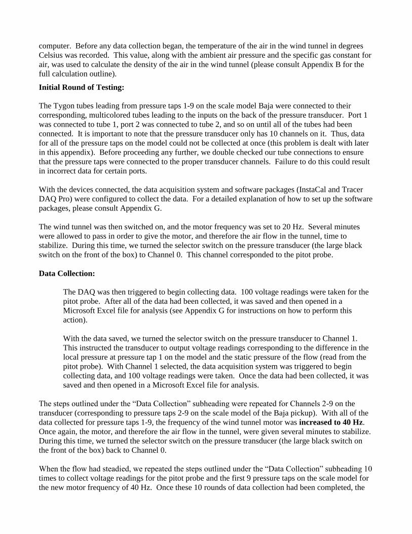
Appendix F

Appendix E contains information about the model used and the locations of the pressure taps on the

model.

MODEL: Baja Pickup Truck

DIMENSIONS: 235 mm long × 90 mm wide × 80 mm tall

i. Top Area = 211.5 cm2

ii. Front Area = 72 cm2

SCALE: 1:12 (i.e. all model dimensions are 1/12 those of the actual dimensions)

Table 5. This table lists the distance each pressure tap is from the front of the model.

Port Number Distance from Front (mm)

1 0

2 30

3 50

4 70

5 85

6 100

7 120

8 140

9 153

10 170

11 190

12 210

13 240

Appendix G

Appendix F contains step-by-step instructions on how to configure the InstaCal and Tracer

DAQ Pro programs for data collection during the experiment.

1) Connect the signal source (the pressure transducer) output to channel 1 (CH1) on the

USB-2408 DAQ. Note the HIGH/LOW inputs for each channel and connect either

voltage output from the transducer.

2) Plug the DAQ into the computer USB port.

3) Start the “InstaCal” program on the computer.

4) Double-click on the board named “#0-USB-2408”.

5) Click the “Flash LED” button. As you click the button, watch for the blinking green

light on the DAQ. If the light flashes, then the DAQ is connected to the computer.

6) Click on “Analog In Channels” to set up inputs.

7) Start the “Tracer DAQ Pro” program on the computer.

8) Click the “Run” button.

9) Select “Edit Channel Settings” and select the number of channels you will use. In

this case, we will only need 1 channel (Channel 1 on the DAQ). Click the “OK” button.

10) Select “Edit Scan Rate Trigger Settings” and select the “None” box.

11) Set your scan rate to 10 samples/second in the “Edit Scan Rate” dropdown menu.

NOTE: The computer may not allow you to set a scan rate of 10

samples/second. If this is the case, change the total scan time under the same

dropdown menu to a total scan time of 16.667 seconds. Then change the scan

rate to 6 samples/second.

12) Click the start button in the upper left-hand corner of the Tracer DAQ Pro window to

begin collecting data. Let the test run its full course before proceeding to step 13.

13) Once the test is complete, select “File Save As” and select “*.txt” in the file type

dropdown menu. Do NOT forget to save the file as a “*.txt” file! Name your file and

save it in a folder that you know how to locate in the computer directory!

14) Start Microsoft Excel.

15) Select “File Open” and double-click on the data file you just saved. Then select

“Delimited Next” and select the box next to “Comma”. Deselect the box next to

“Tab”, and click “Finish”.