Honeycomb-Structured Computational Interconnectsand Their Scalable Extension to Spherical Domains

Joseph B. CessnaComp. Science, Math, & Engineering Program

University of California San DiegoLa Jolla, CA, USA

jcessna@ucsd.edu

Thomas R. BewleyComp. Science, Math, & Engineering Program

University of California San DiegoLa Jolla, CA, USA

bewley@ucsd.edu

ABSTRACTThe present paper is part of a larger effort to redesign, fromtheground up, the best possible interconnect topologies for switchlessmultiprocessor computer systems. We focus here specifically onhoneycomb graphs and their extension to problems on the sphere,as motivated by the design of special-purpose computational clus-ters for global weather forecasting. Eight families of efficient tiledlayouts have been discovered which make such interconnectstriv-ial to scale to large cluster sizes while incorporating no long wires.In the resulting switchless interconnect designs, thephysical prox-imity of the cells created (in the PDE discretization of the physi-cal domain) and thelogical proximityof the nodes to which thesecells are assigned (in the computational cluster) coincideperfectly,so all communication between physically adjacent cells during thePDE simulation require communication over just a single hopinthe computational cluster.

Categories and Subject DescriptorsC.2.1 [Computer-Communication Networks]: Network Archi-tecture and Design—distributed networks, network topology

General TermsDesign

1. INTRODUCTIONThere are two paradigms for interconnecting processing elements

in multiprocessor computer systems: switched and switchless.Switched multiprocessor computer systems are the easiest to field

and use in general-purpose applications, and are thus todaythemost popular. Fast cluster switching hardware has been developedby Infiniband, Myrinet, and Quadrics, and inexpensive (“commod-ity”) switching hardware is available leveraging the standard gi-gabit ethernet protocol from Cisco. Unfortunately, in a switchedcomputer system, the switch itself is a restrictive bottleneck in thesystem when attempting to scale to large cluster sizes, as messagesbetween any two nodes must pass through the switch, and thus thethroughput demands on the switch increase rapidly as the cluster

Permission to make digital or hard copies of all or part of this work forpersonal or classroom use is granted without fee provided that copies arenot made or distributed for profit or commercial advantage and that copiesbear this notice and the full citation on the first page. To copy otherwise, torepublish, to post on servers or to redistribute to lists, requires prior specificpermission and/or a fee.SLIP’09,July 26–27, 2009, San Francisco, California, USA.Copyright 2009 ACM 978-1-60558-576-5/09/07 ...$10.00.

size is increased. Nonuniform memory access (NUMA) architec-tures, first pioneered by Silicon Graphics, attempt to circumventthis quagmire by introducing a hierarchy of switches, thus allow-ing some of the “local” messages (that is, between two nodes onthe same “branch” of a tree-like structure) to avoid passingthroughthe full cascade of switches (that is, to avoid going all the way backto the “trunk”). This NUMA paradigm certainly helps, but does noteliminate the bottlenecks inherent to switch-based architectures.

Switchless multiprocessor computer systems, on the other hand,introduce a “graph” (typically, some sort ofn-dimensional “grid”)to interconnect the nodes of the system. In such a system, messagesbetween any two nodes are relayed along an appropriate path in thegraph, from the source node to the destination node. To accomplishsuch an interconnection in a beowulf cluster, relatively inexpensivePCI cards are available from Dolphin ICS [1]; however, the useof such hardware in today’s high-performance clusters is fairly un-common. The massively parallel high-performance Blue Genede-sign, by IBM, is a switchless three-dimensional torus network withdynamic virtual cut-through routing [2].

In the history of high-performance computing, switchless inter-connect architectures have gone by a variety of descriptivenames,including the 2D torus, the 3D torus, and the hypercube. Almostall such designs, including the IBM Blue Gene and the DolphinICS designs discussed above, imply an underlying Cartesian(thatis, rectangular) grid topology in two, three, orn > 3 dimensions.

Quite recently, the startup SiCortex broke away from the domi-nant Cartesian interconnect paradigm, launching a novel family ofswitchless multiprocessor computer systems designed around theKautz graph [9]. The Kautz graph is the optimal interconnectsolu-tion in terms of connecting the largest number of nodes of a given“degree” (that is, with a given number of incoming and outgoingwires at each node) for any prescribed maximum graph “diame-ter” (that is, the maximum number of hops between any two nodesin the graph). If one considers the wide range of possible graphsthat may be used to interconnect a large number of computationalnodes, the Cartesian graph may be identified as one extreme, withthe simplest local structure possible but a poor graph diameter,whereas the Kautz graph may be considered the other extreme,witha complex logical structure that sacrifices local order but exhibitsthe optimal graph diameter.

In certain unstructured applications, the optimal graph diameteroffered by the Kautz graph is attractive, though such systems be-come difficult to build as the cluster size is increased due totheintricate weave of long wires spanning the entire system.

Many problems of interest in high performance computing, how-ever, have a regular structure associated with them. A primeex-ample is the discretization of a partial differential equation (PDE).When distributing such a discretization on a switchless multipro-

cessor computer systems for its parallel solution, one generallydivides the domain of interest into a number of finite regions, orVoronoi cells, assigning one such cell to each computational node.An important observation is that such computations usuallyrequiremuchmore communication between neighboring cells than they dobetween cells that are physically distant from one another.Thus,the practical effectiveness of proposed solutions to (i) the defini-tion of the Voronoi cells, and (ii) the distribution of thesecells overthe nodes of the cluster (together referred to as the “load balancingproblem”) is closely related to both the physical proximityof thecells created in the PDE discretization and the logical proximity ofthe nodes to which these cells are assigned in the computationalcluster. A graph with local structure, such as the Cartesiangraph,can drastically reduce the average number of hops of the messagesit must pass during the simulation of the PDE by laying out theproblem in such a way that these two proximity conditions coin-cide; a graph without such local structure, such as the Kautzgraph,does not admit an efficient layout which achieves this condition.

The present line of research thus considers alternative (noncar-tesian) graphs with local structure exploitable by PDE discretiza-tions, while keeping to a minimum both (a) the number of wiresper node [to minimize the complexity/expense of the cluster], and(b) the graph diameter [to minimize the cost of whatever multi-hopcommunication is required during the PDE simulation].

This particular paper is motivated by the needs presented byglobal weather forecasting problems defined over a sphere; notethat some of the largest purpose-built computational clusters inthe world are dedicated to this application. Loosely speaking, thepresent paper explores the best ways to put a fine honeycomb gridon a sphere, and then explores how to realize this discretizationefficiently on an easily-scaled layout of computational hardwarewithout using any long wires.

The work considered may be applied immediately at the systemlevel. With the further development of appropriate hardware, itmay also be applied at the board level or even the chip level. Otherchip-level noncartesian interconnect strategies which have been in-vestigated in the literature include the Y architecture andthe X ar-chitecture. The Y architecture for on-chip interconnects is basedon the use of three uniform wiring directions (0o, 120o, and 240o)to exploit on-chip routing resources more efficiently than the tradi-tional Cartesian (a.k.a. Manhattan) wiring architecture [4, 5]. TheX architecture is an integrated-circuit wiring architecture based onthe pervasive use of diagonal wires. Note that, compared with thetraditional Cartesian architecture, the X architecture demonstratesa wire length reduction of more than 20% [11].

2. CARTESIAN INTERCONNECTSTwo criteria by which switchless interconnects are measured are

cluster diameter and maximum wire length [6]. Loosely speaking,the former affects the speed at which information is passed through-out the graph, whereas the latter affects the cost of each wire usedto construct the interconnect, as described further below.

Because each node can communicate directly only with its log-ical neighbors, we characterize information as moving in hops: ittakes one hop for information to travel from a given node to its im-mediate neighbor, two hops for information to travel to a neighborof a neighbor, etc. The diameter of a graph is the maximum numberof hops between any two nodes in the graph. For example, Figure1 illustrates a 1D Cartesian graph with a periodic connection. Eachnode can send information to its neighbor to the right, and receiveinformation from its neighbor to the left. This type of connectionis called a unidirectional link, because information can only flowin one direction. Many switchless clusters use bidirectional links,

1 2 3 4 5 6 7 8

Figure 1: A simple 1D periodic Cartesian interconnect withunidirectional links. The diameter of this graph is seven hops.Note that a long wire is needed to make the periodic connection;the length of this wire increases as the cluster size increases.

1 2 3 4 5 6 7 8

Figure 2: By folding the simple 1D interconnect of Figure 2 inhalf while keeping the same logical connection, the effect of theperiodic connection may be localized. In this case, the longestwires only span the distance between two nodes in the foldedstructure, regardless of the number of nodes in the graph.

Figure 3: By identifying the local structure of the folded 1Din-terconnect of Figure 2, a tile may be designed that contains twonodes and four wires. This tile, together with simple end caps,may be extended to larger interconnects with the same topol-ogy. Here, we extend from 8 nodes (top) to 32 nodes (bottom).

through which a node can both send and receive data.The expense of the hardware required to complete a hop often

increases quickly with the physical length of the wire between thenodes. To reduce this cost, it is thus desirable to minimize themaximum wire length. In Figure 1, the link connecting nodes 1andN traversesN nodes, which makes scaling this layout to largeNcostly. The problem of long wires can be circumvented by foldingthe graph. By keeping the same logical connection, but folding thegraph onto itself along its axis of symmetry, one can producethegraph shown in Figure 2. Here, the interconnect is identicalto thatof Figure 1 (and, thus, so is the graph diameter), but now the longestwire only spans the distance between two nodes, independentof N,thus facilitating scaling of the cluster to largeN.

Noting the repetitive pattern in Figure 2, we identify a self-similartile that can be used to build the interconnect. This tile is composedof two nodes and four wires (two sending and two receiving). Fig-ure 3a illustrates how four of these tiles, along with simpleendcaps, can be combined to produce the original interconnect of Fig-ure 1. An important feature of the tiled configuration is its scalabil-ity; note how it can be extended to much larger interconnectswiththe same topology, such as the 32 node graph in Figure 3b.

We now consider a four-connected periodic 2D Cartesian graph,known as a torus, in which each node has four unidirectional links,two for sending and two for receiving, as illustrated in Figure 4a.Similar to the 1D graph of Figure 1, the diameter of this 2D graphis six hops, but now interconnects 16 nodes instead of 8. The peri-odic connections of this 2D graph create many long wires thatspanthe entire width of the interconnect. These long wires can beelimi-nated by folding the graph onto itself along both axes of symmetry.

From the folded 2D graph, we again identify local structure thatfacilitates tiling. The tiles for the 2D Cartesian torus contain fournodes and the associated communication links. Figure 5 showshow these tiles, together with simple end caps, may be assembled

1 2

3 4

1 2

3 4

1 2

3 4

1 2

3 4

3 34 4

3 34 4

1 212

1 212

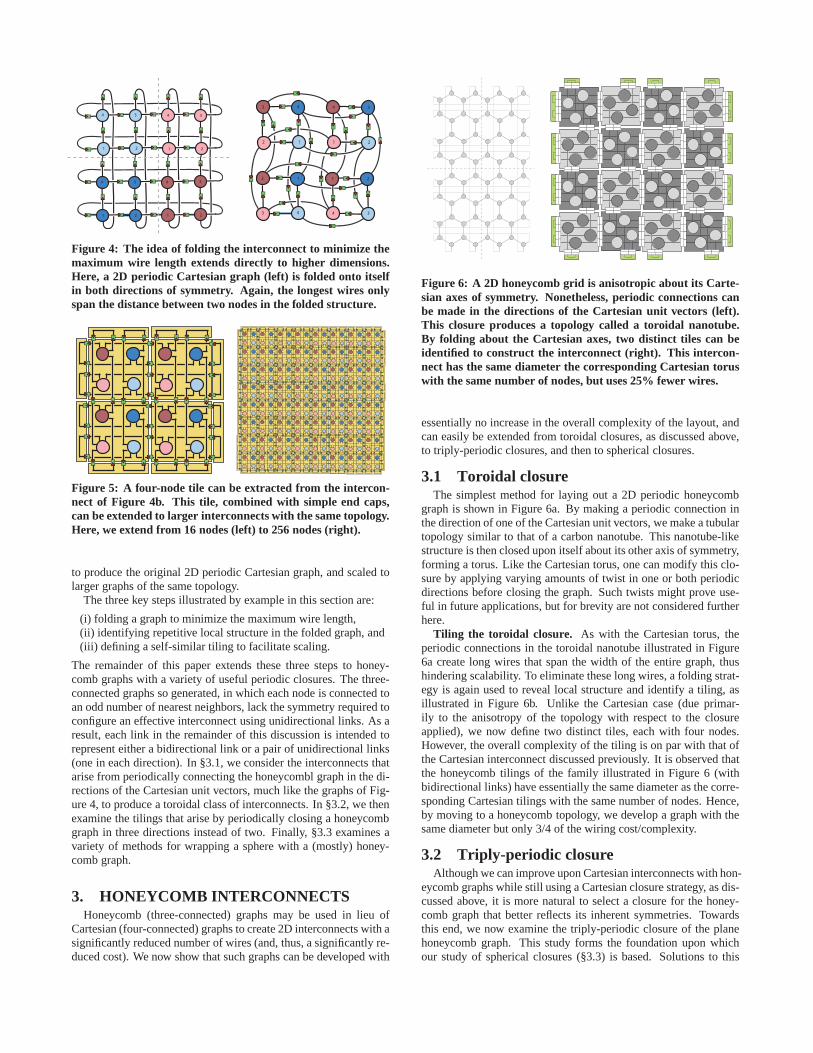
Figure 4: The idea of folding the interconnect to minimize themaximum wire length extends directly to higher dimensions.Here, a 2D periodic Cartesian graph (left) is folded onto itselfin both directions of symmetry. Again, the longest wires onlyspan the distance between two nodes in the folded structure.

Figure 5: A four-node tile can be extracted from the intercon-nect of Figure 4b. This tile, combined with simple end caps,can be extended to larger interconnects with the same topology.Here, we extend from 16 nodes (left) to 256 nodes (right).

to produce the original 2D periodic Cartesian graph, and scaled tolarger graphs of the same topology.

The three key steps illustrated by example in this section are:

a (i) folding a graph to minimize the maximum wire length,a (ii) identifying repetitive local structure in the folded graph, anda (iii) defining a self-similar tiling to facilitate scaling.

The remainder of this paper extends these three steps to honey-comb graphs with a variety of useful periodic closures. The three-connected graphs so generated, in which each node is connected toan odd number of nearest neighbors, lack the symmetry required toconfigure an effective interconnect using unidirectional links. As aresult, each link in the remainder of this discussion is intended torepresent either a bidirectional link or a pair of unidirectional links(one in each direction). In §3.1, we consider the interconnects thatarise from periodically connecting the honeycombl graph inthe di-rections of the Cartesian unit vectors, much like the graphsof Fig-ure 4, to produce a toroidal class of interconnects. In §3.2,we thenexamine the tilings that arise by periodically closing a honeycombgraph in three directions instead of two. Finally, §3.3 examines avariety of methods for wrapping a sphere with a (mostly) honey-comb graph.

3. HONEYCOMB INTERCONNECTSHoneycomb (three-connected) graphs may be used in lieu of

Cartesian (four-connected) graphs to create 2D interconnects with asignificantly reduced number of wires (and, thus, a significantly re-duced cost). We now show that such graphs can be developed with

Figure 6: A 2D honeycomb grid is anisotropic about its Carte-sian axes of symmetry. Nonetheless, periodic connections canbe made in the directions of the Cartesian unit vectors (left).This closure produces a topology called a toroidal nanotube.By folding about the Cartesian axes, two distinct tiles can beidentified to construct the interconnect (right). This intercon-nect has the same diameter the corresponding Cartesian toruswith the same number of nodes, but uses 25% fewer wires.

essentially no increase in the overall complexity of the layout, andcan easily be extended from toroidal closures, as discussedabove,to triply-periodic closures, and then to spherical closures.

3.1 Toroidal closureThe simplest method for laying out a 2D periodic honeycomb

graph is shown in Figure 6a. By making a periodic connection inthe direction of one of the Cartesian unit vectors, we make a tubulartopology similar to that of a carbon nanotube. This nanotube-likestructure is then closed upon itself about its other axis of symmetry,forming a torus. Like the Cartesian torus, one can modify this clo-sure by applying varying amounts of twist in one or both periodicdirections before closing the graph. Such twists might prove use-ful in future applications, but for brevity are not considered furtherhere.

Tiling the toroidal closure. As with the Cartesian torus, theperiodic connections in the toroidal nanotube illustratedin Figure6a create long wires that span the width of the entire graph, thushindering scalability. To eliminate these long wires, a folding strat-egy is again used to reveal local structure and identify a tiling, asillustrated in Figure 6b. Unlike the Cartesian case (due primar-ily to the anisotropy of the topology with respect to the closureapplied), we now define two distinct tiles, each with four nodes.However, the overall complexity of the tiling is on par with that ofthe Cartesian interconnect discussed previously. It is observed thatthe honeycomb tilings of the family illustrated in Figure 6 (withbidirectional links) have essentially the same diameter asthe corre-sponding Cartesian tilings with the same number of nodes. Hence,by moving to a honeycomb topology, we develop a graph with thesame diameter but only 3/4 of the wiring cost/complexity.

3.2 Triply-periodic closureAlthough we can improve upon Cartesian interconnects with hon-

eycomb graphs while still using a Cartesian closure strategy, as dis-cussed above, it is more natural to select a closure for the honey-comb graph that better reflects its inherent symmetries. Towardsthis end, we now examine the triply-periodic closure of the planehoneycomb graph. This study forms the foundation upon whichour study of spherical closures (§3.3) is based. Solutions to this

A1 A2 A6

Figure 7: Three ClassA structures (that is, honeycomb graphson the equilateral triangle) with degree = 1, 2, and 6.

B1 B2 B4

Figure 8: Three ClassB structures with degree = 1, 2, and 4.

PA2 PB1

Figure 9: The two families of triply-periodic honeycomb inter-connects. ThePA∗ family is built from six Class A structuresand has connected edge links whereas thePB∗ family is builtfrom six ClassB structures and has coincident edge nodes.

problem build from two distinct classes of honeycomb graphsonthe equilateral triangle, denoted in this work as ClassA and ClassB structures:

A) The ClassA structures place the midpoints of the links on theedges of the equilateral triangle, as illustrated in Figure7. The de-gree of this structure is defined as the number of midpoints that lieon each edge of the triangle.

B) The ClassB structures place the edges of the hexagons on theedges of the equilateral triangle, as illustrated in Figure8. The de-gree of this structure is defined as the number of hexagons touchingeach edge of the triangle.

It is straightforward to join six ClassA or ClassB structures, as il-lustrated in Figures 7 and 8, to form a hexagon, as illustrated in Fig-ure 9. The periodic connections on this hexagon are easily applied:in the case of ClassA, the wires on opposite sides of the hexagonare connected; in the case of ClassB, the nodes on opposite sides ofthe hexagon are taken to be identical (in both cases, moving orthog-onal to each side of the hexagon, not diagonally through the centerpoint). The resulting graphs are denotedPA∗ andPB∗, where the∗ denotes the degree of the six ClassA or ClassB structures fromwhich the triply-periodic honeycomb graph is built.

Tiling the triply-periodic closure. As in the previous exam-ples, the triply-periodic graphs of Figure 9 can be tiled viafoldingabout the three axes of symmetry and identifying the repetitive lo-cal structure of the folded graph. This process eliminates all longwires which grow as the graph size is increased. For ClassA, thenew tile so constructed, denoted TileE in Figure 10, contains sixnodes instead of four, leading to the tiledPA∗ family illustrated in

EF

G

Figure 10: The three fundamental tiles, denotedE, F , and G,upon which the tilings of the triply-periodic (§3.2) and spheri-cal (§3.3) closures of the honeycomb interconnect are based.

T O I

Figure 11: The three Platonic solids with triangular faces.From left to right: Tetrahedron (4 faces), Octahedron (8 faces),and Icosahedron (20 faces). The faces of these polyhedra canbe gridded with either ClassA or ClassB triangular graphs (seeFigures 7 and 8) to build tiled spherical interconnects based onthe fundamental tiles introduced in Figure 10.

the first four subfigures of Figure 18. For ClassB, the new tile soconstructed contains 18 nodes; as illustrated in the last four subfig-ures of Figure 18, and for later convenience, we may immediatelysplit this 18-node tile into three identical smaller tiles,denoted TileF in Figure 10. The tilings are completed with simple end caps.

3.3 Spherical closureWe now discuss the most uniform techniques available to cover

a sphere with a (mostly) honeycomb grid.Note first that eachAn structure of Figure 7 hasV = n2 vertices

(that is, nodes) andE = 1.5n2 edges (that is, wires between nodes),whereas eachBn structure of Figure 8 hasV = 3n2 vertices andE = 4.5n2 edges. If each corner of anAn structure is joined withfive other identicalAnstructures, then eachAnstructure contributeseffectivelyF = 0.5n2 faces (that is, hexagons) to the overall graph,whereas if each corner of aBn structure is joined with five otherBn structures, then eachBn structure contributesF = 1.5n2 facesto the overall graph. In both cases, we haveV −E +F = 0, whichis characteristic of a planar graph.

Euler’s formulaV −E + F = 2 relates the numbers of vertices,edges, and faces of any convex polyhedron. The upshot of Eu-ler’s formula in the present problem is that it is impossibleto covera sphere perfectly with a honeycomb grid. By this formula, anyattempt to map a honeycomb grid onto the sphere will lead to a pre-dictable number of “defects” (that is, faces which are not hexagons).

The three most uniform constructions available for generating amostly honeycomb graph on a sphere are given by pasting a set ofidentical An structures of Figure 7, orBn structures of Figure 8,onto the triangular faces of a Tetrahedron, Octahedron, or Icosahe-dron (see Figure 11); these three constructions form the basis forthe remainder of this study. Note that this approach joins each cor-ner of the structure selected with two, three, or four other identicalstructures, and leads to 4 triangular faces, 6 square faces,or 12pentagonal faces embedded within an otherwise honeycomb graph.The resulting graph is easily projected onto the sphere. Allgraphsso constructed, of course, satisfy Euler’s formula. Some ofthegraphs so constructed occur in nature as nearly spherical carbonmolecules known as Buckyballs.

Deg

ree Symmetry and Class

Periodic Tetrahedral Octahedral IcosahedralA B A B A B A B

1 6 18 4 12 8 24 20 602 24 72 16 48 32 96 80 2403 54 162 36 108 72 216 180 5404 96 288 64 192 128 384 320 960...

......

......

......

......

k 6k2 18k2 4k2 12k2 8k2 24k2 20k2 60k2

Table 1: Number of nodes in a honeycomb interconnect. Forthe same symmetry and degree, the ClassB topologies havethree times as many nodes as ClassA. Note also thatOA1 is acube,IA1 is a dodecahedron, andIB1 is a buckminsterfullerene.

Table 1 shows the number of nodes in these graphs as a functionof their symmetry (P, T, O, or I ), class (A or B), and degree (k).For each case, the number of nodes increases withk2. For a givensymmetry and degree, the ClassB graph contains three times asmany nodes as the ClassA graph.

For general-purpose computing on switchless multiprocessor com-puter systems, spherical interconnects (§3.3) are not quite as ef-ficient as planar interconnects (§3.2) with either toroidalclosureor triply-periodic closure, as spherical interconnects have slightlyhigher diameters for a given number of nodes. However, as men-tioned previously, spherical interconnects are poised to make a ma-jor impact for the specific problem of solving PDEs on the sphere,which is an important class of computational grand challenge prob-lems central to a host of important questions related to global wea-ther forecasting, climate prediction, and solar physics. In fact, someof the largest purpose-built supercomputers in the world are dedi-cated to such applications, and thus it is logical to design somecomputational clusters with switchless interconnects which are nat-urally suited to this particular class of applications.

Some of the graphs developed here lend themselves particularlywell to efficient numerical solution of elliptical PDEs via the iter-ative geometric multigrid method; Figure 12 illustrates six graphsthat may be used for such a purpose (OA2p for p = {0,1, · · · ,5}).Note that the Octahedral symmetry of these grids introducesa keyproperty missing from the Tetrahedral and Icosahedral families ofspherical interconnects: due to the square defect regions of theOctahedral graphs, a red/black ordering of points is maintainedover the entire graph. That is, half of the points may be labeledas red and the other half labeled as black, with red points hav-ing only black neighbors and black points having only red neigh-bors. This ordering allows an iterative smoothing algorithm knownas Red/Black Gauss Seidel to be applied at each sub step of themultigrid algorithm and facilitates remarkable multigridconver-gence rates and efficient scaling on multiprocessor machines tovery large grids.

Although the idea of building the interconnect of a multiproces-sor computer system in the form of a honeycomb spherical graph isstill in its infancy, people have known about and used such graphsto discretize the sphere in the numerical weather prediction com-munity for many years; see, e.g., [3], [8], and [10]. In particular, themodel developed by the Deutscher Wetterdienst (DWD) is an ex-ample of an operational meteorological code that implements thedual of a honeycomb graph with icosahedral symmetry (see [7]).These previous investigations have almost exclusively used graphswith Icosahedral symmetry, as such graphs undergo the leastdefor-mation when being projected from the polyhedron (on which they

OA1 OA2 OA4

OA8 OA16 OA32

Figure 12: A representative family of spherical interconnects.All six graphs are members of theOA2p family (three of thesquare “defect" regions are visible in each graph). From top-left to bottom-right the degree is 20,21,22,23,24, and 25. Thethick black lines show the logical interconnect. The light greylines illustrate the respective Voronoi cell for each node,indi-cating the region of the physical domain that each node is re-sponsible for in a PDE simulation on a sphere.

are built) onto the sphere (where they are applied). Minimizingsuch graph deformation is beneficial for improving accuracyin nu-merical simulations. However, as mentioned above, our researchindicates that Octahedral graphs, which admit a valuable red/blackordering not available in Icosahedral graphs, might, on balance,prove to be significantly better suited in many applications.

Tiling the spherical closure. As illustrated in Figure 12, spher-ical graphs are quite complicated; their practical deployment forlargeN would be quite difficult without a scalable tiling strategy.Thus, in a manner analogous to that used in §3.1 and §3.2, we nowtransform these graphs to discover local patterns and identify self-similar tilings that make such constructions tractable andscalable.

To illustrate the process, consider first theTB2 interconnect as arepresentative example, as depicted in Figure 13. Note firstthat wereplace the “folding” idea used in §2, §3.1, and §3.2 with a “stretch-ing” and “grouping” strategy. The stretching step may be visualizedby imagining all links in the spherical graph under consideration aselastic, then imagining the transformation that would result fromgrabbing all of the nodes near one of the vertices of the polyhe-dron, or near the center of one of the faces of the polyhedron,andpulling them out to the side (while maintaining the connectivity)until the resulting stretched graph may be laid flat. The resultingspider web-like structure is known as a Schlegel diagram.

For theTB2 Schlegel diagram in the top-right of Figure 13, theouter edge of the diagram is a triangle that corresponds to the nodesnear one of the vertices of the tetrahedron of the unstretched graph,and near the center of the diagram is a hexagon that corresponds tonodes near the middle of the opposite face of the tetrahedron.

The next step in tiling a spherical graph is to identify repetitivestructure. In the Schlegel diagram of Figure 13, after considerabledeliberation, we have grouped the nodes in sets of six. This group-ing is not unique, but it is with the choice shown that a simpletiledstructure reveals itself. In general, nodes that are approximatelythe same distance from the center of the Schlegel diagram tend tobe lumped together. From the selected grouping, we can create theflowchart shown on the lower-left of Figure 13. In this flowchart,all obvious honeycomb structure is removed, but now the groups of

TB2

TB2 TB2

TB2Tiling

Schlegelgraph

flowchart

Figure 13: In order to determine a tiling for a given sphericalinterconnect graph (top-left), a Schlegel diagram (top-right) isfirst constructed by stretching and flattening the graph ontotheplane while maintaining the same logical connections. Fromthis, locally similar groups of nodes can be grouped into arevealing “flowchart” (bottom-left) that ultimately makes thetiling evident (bottom-right). In the case of TB2 illustratedhere, with the exception of the top of each column of theflowchart, the nodes are connected identically to thePA∗ case,leading to a tiling with the E tiles of Figure 10. This tiling isthen completed withF tiles from Figure 10 along one side, to-gether with the appropriate end caps.

paired nodes are brought together in what will eventually becometheir tiled form. Significantly, the logical structure of the flowchart(as well as the Schlegel diagram) is identical to the original spheri-cal interconnect. Note that flow from bottom to top on the flowchartcorresponds to in-to-out flow in the Schlegel diagram.

With the exception of the top set of nodes in each column ofthe flowchart, the connections between the other six sets of nodesmatch those of thePA∗ case. That is, the first node in each groupis connected to the first node in the neighboring groups, etc.As aresult, we can use the sameE tiles (see Figure 10) to construct thispart of the graph as were used in thePA∗ constructions. The re-maining two sets of nodes can be incorporated using theF tile usedin the PB∗ constructions. After making simple end connections,the completed tiling is shown on the bottom-right of Figure 13. Inthis case, the overall tiling builds out to a right triangle.

For each interconnect family, we perform a similar procedurefor the first few graph degrees until a pattern emerges, first stretch-ing/flattening the graph to make a Schlegel diagram, then identify-ing repetitive local structure by grouping the nodes in an in-to-outflowchart of the Schlegel diagram, and finally defining a tiling tofacilitate scaling. Though this was an involved process, byso do-ing, we have discovered the simple and easily scaled families oftilings depicted in Figures 19 - 21.

Interesting and surprising correlations exist between thevarioussimple tilings which we have discovered. We first observe that eachsymmetry family shares a common overall shape: theT ∗∗ familybuilds out to right triangles, theO∗∗ family builds out to parallelo-grams, and theI ∗∗ family builds out to “six-sided parallelograms”.

By identifying an equivalence between a pair ofE tiles and apair ofF tiles, as depicted in Figure 14, we are also able to identifyinterfamily relationships between the tilings as well. Applying this

Figure 14: An equivalence between a pair ofE tiles and a pairof F tiles. Typically, we use theE tiles whenever possible; how-ever, the equivalence between these two pairings helps to unifythe ClassB tilings of the various different families.

Figure 15: For any of the OB∗ family of tilings (here, OB1 isshown), we can replace theE tiles along the shorter diagonalusing the equivalence depicted in Figure 14. This allows usto identify the bifurcation axis that splits the tiling into twosmaller tilings in the TB∗ tilings of the appropriate degree.

Figure 16: (left) The IBn graph may be subdivided into foursmaller tilings [two TBn and two PBn] via a series of simpleswitches applied to the electrical connections between thetilesalong the three diagonals shown; a similar subdivision to foursmaller tilings [two TAn and two PAn] may also be accom-plished with the IAn tiling after the transformation illustratedin Figure 14 is applied along the appropriate diagonals. (right)The IBn tiling, for n even, may also be subdivided a differentway [to two TBn and two OA(n/2)]; a similar subdivision [totwo TAnand two OB(3n/2)] may also be accomplished with theIAn tiling, for n even, after the transformation in Figure 14 isapplied appropriately. Such subdivisions are useful for runningfour small jobs on the cluster simultaneously.

substitution along the shortest diagonal of theOB∗ family, as illus-trated in Figure 15, shows immediately how theOB∗ tiling can bebuilt up from two tilings of theTB∗ family. Equivalently, theOA∗family can be built from twoTA∗ tilings of the appropriate degree.

Similarly, as illustrated in Figure 16, theI ∗∗ family of tilings canbe built up from twoT ∗∗ tilings and either twoP∗∗ tilings or twoO∗ ∗ tilings. Such subdivisions could be useful for running foursmaller jobs on the cluster simultaneously without reconfiguration.

We have focused in §3.3 on applying the triangular ClassA andClassB structures from Figures 7 and 8 to the triangular faces ofthree of the Platonic solids (Figure 11). However, other construc-tions are also possible. For instance, the truncated tetrahedron (Fig-ure 17) has only hexagonal and triangular sides, and thus canbecovered with triangular ClassA or ClassB structures on its triangu-lar faces and six ClassA or ClassB structures (see Figure 9) on itshexagonal sides. The resulting ClassAgraphs have 28k2 nodes, andthe resulting ClassB graphs have 84k2 nodes (cf. Table 1). Thesegraphs each have 12 pentagonal faces embedded within an other-wise honeycomb graph, just like the icosahedron; however, oneprojected out to the sphere, they are slightly less uniform and do notadmit a red/black ordering of points. Another alternative construc-

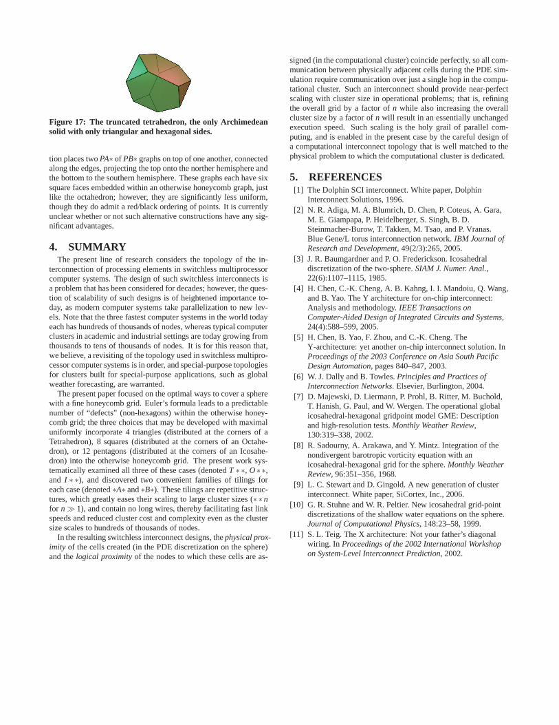
Figure 17: The truncated tetrahedron, the only Archimedeansolid with only triangular and hexagonal sides.

tion places twoPA∗ of PB∗ graphs on top of one another, connectedalong the edges, projecting the top onto the norther hemisphere andthe bottom to the southern hemisphere. These graphs each have sixsquare faces embedded within an otherwise honeycomb graph,justlike the octahedron; however, they are significantly less uniform,though they do admit a red/black ordering of points. It is currentlyunclear whether or not such alternative constructions haveany sig-nificant advantages.

4. SUMMARYThe present line of research considers the topology of the in-

terconnection of processing elements in switchless multiprocessorcomputer systems. The design of such switchless interconnects isa problem that has been considered for decades; however, theques-tion of scalability of such designs is of heightened importance to-day, as modern computer systems take parallelization to newlev-els. Note that the three fastest computer systems in the world todayeach has hundreds of thousands of nodes, whereas typical computerclusters in academic and industrial settings are today growing fromthousands to tens of thousands of nodes. It is for this reasonthat,we believe, a revisiting of the topology used in switchless multipro-cessor computer systems is in order, and special-purpose topologiesfor clusters built for special-purpose applications, suchas globalweather forecasting, are warranted.

The present paper focused on the optimal ways to cover a spherewith a fine honeycomb grid. Euler’s formula leads to a predictablenumber of “defects” (non-hexagons) within the otherwise honey-comb grid; the three choices that may be developed with maximaluniformly incorporate 4 triangles (distributed at the corners of aTetrahedron), 8 squares (distributed at the corners of an Octahe-dron), or 12 pentagons (distributed at the corners of an Icosahe-dron) into the otherwise honeycomb grid. The present work sys-tematically examined all three of these cases (denotedT ∗∗, O∗∗,and I ∗ ∗), and discovered two convenient families of tilings foreach case (denoted∗A∗ and∗B∗). These tilings are repetitive struc-tures, which greatly eases their scaling to large cluster sizes (∗ ∗nfor n≫ 1), and contain no long wires, thereby facilitating fast linkspeeds and reduced cluster cost and complexity even as the clustersize scales to hundreds of thousands of nodes.

In the resulting switchless interconnect designs, thephysical prox-imity of the cells created (in the PDE discretization on the sphere)and thelogical proximityof the nodes to which these cells are as-

signed (in the computational cluster) coincide perfectly,so all com-munication between physically adjacent cells during the PDE sim-ulation require communication over just a single hop in the compu-tational cluster. Such an interconnect should provide near-perfectscaling with cluster size in operational problems; that is,refiningthe overall grid by a factor ofn while also increasing the overallcluster size by a factor ofn will result in an essentially unchangedexecution speed. Such scaling is the holy grail of parallel com-puting, and is enabled in the present case by the careful design ofa computational interconnect topology that is well matchedto thephysical problem to which the computational cluster is dedicated.

5. REFERENCES[1] The Dolphin SCI interconnect. White paper, Dolphin

Interconnect Solutions, 1996.[2] N. R. Adiga, M. A. Blumrich, D. Chen, P. Coteus, A. Gara,

M. E. Giampapa, P. Heidelberger, S. Singh, B. D.Steinmacher-Burow, T. Takken, M. Tsao, and P. Vranas.Blue Gene/L torus interconnection network.IBM Journal ofResearch and Development, 49(2/3):265, 2005.

[3] J. R. Baumgardner and P. O. Frederickson. Icosahedraldiscretization of the two-sphere.SIAM J. Numer. Anal.,22(6):1107–1115, 1985.

[4] H. Chen, C.-K. Cheng, A. B. Kahng, I. I. Mandoiu, Q. Wang,and B. Yao. The Y architecture for on-chip interconnect:Analysis and methodology.IEEE Transactions onComputer-Aided Design of Integrated Circuits and Systems,24(4):588–599, 2005.

[5] H. Chen, B. Yao, F. Zhou, and C.-K. Cheng. TheY-architecture: yet another on-chip interconnect solution. InProceedings of the 2003 Conference on Asia South PacificDesign Automation, pages 840–847, 2003.

[6] W. J. Dally and B. Towles.Principles and Practices ofInterconnection Networks. Elsevier, Burlington, 2004.

[7] D. Majewski, D. Liermann, P. Prohl, B. Ritter, M. Buchold,T. Hanish, G. Paul, and W. Wergen. The operational globalicosahedral-hexagonal gridpoint model GME: Descriptionand high-resolution tests.Monthly Weather Review,130:319–338, 2002.

[8] R. Sadourny, A. Arakawa, and Y. Mintz. Integration of thenondivergent barotropic vorticity equation with anicosahedral-hexagonal grid for the sphere.Monthly WeatherReview, 96:351–356, 1968.

[9] L. C. Stewart and D. Gingold. A new generation of clusterinterconnect. White paper, SiCortex, Inc., 2006.

[10] G. R. Stuhne and W. R. Peltier. New icosahedral grid-pointdiscretizations of the shallow water equations on the sphere.Journal of Computational Physics, 148:23–58, 1999.

[11] S. L. Teig. The X architecture: Not your father’s diagonalwiring. In Proceedings of the 2002 International Workshopon System-Level Interconnect Prediction, 2002.

PA1

PA4

PA2

PA3

PB1

PB4

PB2

PB3

Figure 18: The first four members of thePA∗ and PB∗ families of interconnects; each builds out to an equilateral triangle. Note thatthe PA∗ construction illustrated here is built using E tiles, whereas thePB∗ construction is built using F tiles (see Figure 10).

TA1TA2

TA3

TA4

TB1

TB2

TB3

TB4

Figure 19: The first four members of theTA∗ and TB∗ families of interconnects; each builds out to a right triangle.

OA1

OA2

OA3

OA4

OB1

OB2

OB3

OB4

Figure 20: The first four members of theOA∗ and OB∗ families of interconnects; each builds out to a parallelogram. Both familiesmay be constructed by connecting twoTA∗ or TB∗ tilings along the longest leg, as described in Figure 15.

IA1 IA2

IA3

IA4

IB1 IB2

IB3

IB4

Figure 21: The first four members of theIA∗ and IB∗ families of interconnects; each builds out to a “six-sided parallelogram”. Bothfamilies may be constructed by connecting twoT ∗∗ and two P∗∗ tilings, or two T ∗∗ and two O∗∗ tilings, as described in Figure 16.