Honey Bee Social Foraging Algorithms for

Resource Allocation: Theory and ApplicationNicanor Quijano, Student Member, IEEE, and Kevin M. Passino, Fellow, IEEE

Abstract

A model of honey bee social foraging is introduced to create an algorithm that solves a class of

optimal resource allocation problems. We prove that if several such algorithms (“hives”) compete in the

same problem domain, the strategy they use is a Nash equilibirium and an evolutionarily stable strategy.

Moreover, for a single or multiple hives we prove that the allocation strategy is globally optimal. To

illustrate the practical utility of the theoretical results and algorithm we show how it can solve a dynamic

voltage allocation problem to achieve a maximum uniformly elevated temperature in an interconnected

grid of temperature zones.

Index Terms

Ideal free distribution, honey bee social foraging, evolutionarily stable strategy, dynamic resource

allocation, temperature control

The authors would like to thank NIST for support for development of the temperature control experiment. Also, we wouldlike to thank the OSU office of Research for partial financial support via an interdisciplinary research grant.

The authors are with the Department of Electrical and Computer Engineering, The Ohio State University, 2015 Neil Avenue,Columbus Ohio, 43210, USA (e-mail: quijano.2@osu.edu; passino@ece.osu.edu).

1

Honey Bee Social Foraging Algorithms for

Resource Allocation: Theory and Application

I. INTRODUCTION

Evolution by natural selection has shaped biosystem optimization and control processes to enhance the

probability of species survival [1]. The “bioinspired” design approach [2] seeks to exploit the evolved

“tricks” of nature to construct robust high performance technological solutions. For instance, the ant

colony optimization (ACO) algorithms introduced by M. Dorigo and colleagues (e.g., see [3]–[6]) mimic

ant foraging behavior and have been used in the solution to classical optimization problems (e.g., discrete

combinatorial optimization problems [7]) and in engineering applications (e.g., [8], [9]). The primary

goal of this paper is to show that honey bee social foraging techniques can be exploited in a bioinspired

design approach to (i) solve a continuous optimization problem underlying resource allocation [10],

and (ii) provide novel strategies for multizone temperature control, an important industrial engineering

application.

Our model of honey bee social foraging relies on experimental studies [11] and some ideas from other

mathematical models of the process. A differential equation model of functional aspects of dynamic labor

force allocation of honey bees is developed and validated for one set of experimental conditions in [1],

[12]. The work in [13] extends this model (e.g., by adding details on energetics and currency) and [14]

introduced a generic nonlinear differential equation model that can represent social foraging processes in

both bees and ants. Like in [13], [14], our model of recruitment uses the idea from [1], [12] that dance

strength proportioning on the dance floor shares some characteristics with the evolutionary process (e.g.,

with fitness corresponding to forage site profitability and reproduction to recruitment as discussed in [11]).

Here we make such connections more concrete by modeling the bee recruitment process in an analogous

manner to how survival of the fittest and natural selection are modeled in genetic algorithms using a

stochastic process of fitness proportionate selection [15]. The authors in [16] introduce an “individual-

oriented” model of social foraging and validate it against one set of experimental conditions as was done

in [1], [12]. More recently, in [17] the authors expanded and improved the model in [16] (e.g., taking into

account the findings in [18] and by studying an equal harvest rate forager allocation distribution). The

work in [19] studies the pattern of forager allocation and the optimality of it. The authors in [20] study

the spatial distribution of solitary and social food provisioners under different currency assumptions. The

2

work in [17], [19], [20] identifies connections to the concept of the “ideal free distribution” (IFD) [21].

Here, we do not use a detailed characterization of bee and nectar energetics and currency since there is

not enough experimental evidence to justify whether or when a gathering rate or efficiency-based currency

is used [11]; instead, we develop a generic measure of forage site profitability. This general profitability

measure approach is the same one used in [22] to represent the nest-site quality landscape for the honey

bee nest-site selection process. Our general measure has the advantage of allowing us to easily represent

a wide range of density-dependent foraging currencies via the classical “suitability function” approach

to IFD studies [21]. Also, it eases the transition to the multizone temperature control problem since the

temperature control objective can be easily characterized with our general profitability measure.

The IFD concept has been used to analyze how animals distribute themselves across different habitats

or patches of food [21]. These habitats have different characteristics (e.g., one habitat might have a higher

nutrient input rate than another), but animals tend to reach an equilibrium point where each has the same

correlate of fitness (e.g., consumption rate). The term “ideal” means that the animals can perfectly sense

the quality of all habitats and seek to maximize the suitability of the habitat they are in (by choosing

which habitat to reside in), and the term “free” means that the animals can go to any habitat. In this paper,

the IFD is a central unifying concept. The IFD will emerge for one hive as the foragers are cooperatively

allocated across sites. Moreover, if n hives compete in the same environment for a resource the IFD

will also emerge. Here, we create a mathematical representation of the n-hive game where each hive’s

strategy choice entails picking the distribution of its foragers across the environment. Our analytical study

starts by showing that the IFD is a strict Nash equilibrium [23] in terms of the payoffs to each hive and

a special type of evolutionarily stable strategy (ESS). The original definition of an ESS is based on one

important assumption: the population size has to be infinite. In [24], [25] the authors define the conditions

that must be satisfied in order to prove that a strategy is evolutionarily stable for a finite-population size.

Using the ideas in [24] we state the conditions for what we call a one-stable ESS, and show that the

IFD satisfies those conditions. This means that in an n-hive game, if a single hive’s strategy (forager

allocation) mutates from the IFD it cannot survive when competing against a field of n − 1 hives that

use the IFD strategy. While this means that the IFD is locally optimal in a game-theoretic sense (i.e.,

unilateral forager allocation deviations by a hive are not profitable), here we show that the achieved IFD

is a global optimum point for both single hive and n-hive allocations. For the n-hive case, this means

that if the forager allocation of all hives but one is at the IFD, then the remaining hive has to distribute

its effort according to the IFD if it is to maximize its return.

The utility of these theoretical concepts and the honey bee social foraging algorithm are illustrated by

3

means of an engineering application. One possible engineering application is the dynamical allocation of

servers on the Internet [26]. However, the technological challenge we confront is multizone temperature

control. Achievement of high performance multizone temperature control is very important in a range of

commercial and industrial applications. For instance, recent work in this area includes distributed control

of thermal processes [27]–[31], and semiconductor processing [32]–[34]. Particularly relevant to our work

is the study in [29], where the authors use multivariable distributed control in order to maintain a uniform

temperature across a wafer during ramp-up (similar to the control objective we study here). In [35] the

authors describe a lithographical system that is heated by 49 independently controlled zones. Here, we

use a multizone experimental setup that is similar to the one in [36] where dynamic resource allocation

methods are studied. Our experiments demonstrate how one hive can achieve an IFD that corresponds

to maximum uniform temperatures on the temperature grid. We illustrate the dynamics of the foraging

algorithm by showing how it can successfully eliminate the effects of ambient temperature disturbances.

Moreover, we show that even if two hives have imperfect information they can be used as a feedback

control that will still achieve an IFD.

The paper is organized as follows. First, in Section II we introduce the honey bee social foraging

algorithm. In Section III we perform a theoretical analysis of the hives’ achieved IFD equilibrium.

In Section IV we apply the honey bee social foraging algorithm to a multizone temperature control

experiment and show how the IFD emerges under a variety of conditions.

II. HONEY BEE SOCIAL FORAGING ALGORITHM

Modeling social foraging for nectar involves representing the environment, activities during bee ex-

peditions (exploration and foraging), unloading nectar, dance strength decisions, explorer allocation,

recruitment on the dance floor, and accounting for interactions with other hive functions. The experimental

studies we rely on are summarized in [11]. Our primary sources for constructing components of our model

are as follows: dance strength determination, dance threshold, and unloading area [18], [37], [38]; dance

floor and recruitment rates [12]; and explorer allocation and its relation to recruitment [39], [40].

A. Foraging Profitability Landscape

We assume that there are a fixed number of B bees involved in foraging. For i = 1, 2, ..., B bee

i is represented by θi ∈ �2 which is its position in two-dimensional space. During foraging, bees

sample a “foraging profitability landscape” which we think of as a spatial distribution of forage sites

with encoded information on foraging profitability that quantifies distance from hive, nectar sugar content,

4

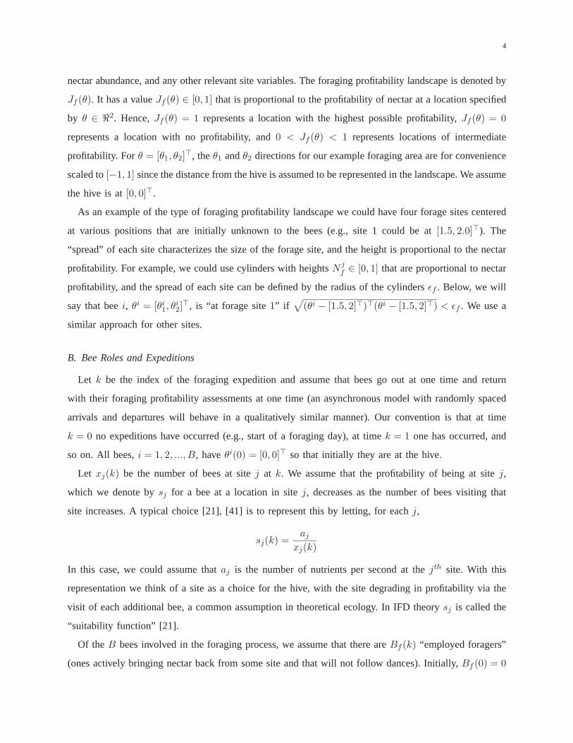
nectar abundance, and any other relevant site variables. The foraging profitability landscape is denoted by

Jf (θ). It has a value Jf (θ) ∈ [0, 1] that is proportional to the profitability of nectar at a location specified

by θ ∈ �2. Hence, Jf (θ) = 1 represents a location with the highest possible profitability, Jf (θ) = 0

represents a location with no profitability, and 0 < Jf (θ) < 1 represents locations of intermediate

profitability. For θ = [θ1, θ2]�, the θ1 and θ2 directions for our example foraging area are for convenience

scaled to [−1, 1] since the distance from the hive is assumed to be represented in the landscape. We assume

the hive is at [0, 0]�.

As an example of the type of foraging profitability landscape we could have four forage sites centered

at various positions that are initially unknown to the bees (e.g., site 1 could be at [1.5, 2.0]�). The

“spread” of each site characterizes the size of the forage site, and the height is proportional to the nectar

profitability. For example, we could use cylinders with heights N jf ∈ [0, 1] that are proportional to nectar

profitability, and the spread of each site can be defined by the radius of the cylinders εf . Below, we will

say that bee i, θi = [θi1, θ

i2]�, is “at forage site 1” if

√(θi − [1.5, 2]�)�(θi − [1.5, 2]�) < εf . We use a

similar approach for other sites.

B. Bee Roles and Expeditions

Let k be the index of the foraging expedition and assume that bees go out at one time and return

with their foraging profitability assessments at one time (an asynchronous model with randomly spaced

arrivals and departures will behave in a qualitatively similar manner). Our convention is that at time

k = 0 no expeditions have occurred (e.g., start of a foraging day), at time k = 1 one has occurred, and

so on. All bees, i = 1, 2, ..., B, have θi(0) = [0, 0]� so that initially they are at the hive.

Let xj(k) be the number of bees at site j at k. We assume that the profitability of being at site j,

which we denote by sj for a bee at a location in site j, decreases as the number of bees visiting that

site increases. A typical choice [21], [41] is to represent this by letting, for each j,

sj(k) =aj

xj(k)

In this case, we could assume that aj is the number of nutrients per second at the jth site. With this

representation we think of a site as a choice for the hive, with the site degrading in profitability via the

visit of each additional bee, a common assumption in theoretical ecology. In IFD theory sj is called the

“suitability function” [21].

Of the B bees involved in the foraging process, we assume that there are Bf (k) “employed foragers”

(ones actively bringing nectar back from some site and that will not follow dances). Initially, Bf (0) = 0

5

since no foraging sites have been found. We assume that there are Bu(k) = Bo(k)+Br(k) “unemployed

foragers” with Bo(k) that seek to observe the dances of employed foragers on the dance floor and Br(k)

that rest (or are involved in some other activity). Initially, Bu(0) = B, which with the rules for resting

and observing given below will set the number of resters and observers. We assume that there are Be(k)

“forage explorers” that go to random positions in the environment, bring their nectar back if they find

any, and dance accordingly, but were not dedicated to the site (of course they may become dedicated if

they find a relatively good site).

We ignore the specific path used by the foragers on expeditions and what specific activities they

perform. We assume that a bee simply samples the foraging profitability landscape once on its expedition

and hence this sample represents its combined overall assessment of foraging profitability for location

θi(k). It is this value that it holds when it returns to the hive. It also brings back knowledge of the forage

location which is represented with θi(k) for the kth foraging expedition. Let the foraging profitability

assessment by employed forager (or forage explorer) i be

F i(k) =

⎧⎪⎪⎪⎨⎪⎪⎪⎩

1 if Jf (θi(k)) + wif (k) ≥ 1

Jf (θi(k)) + wif (k) if 1 > Jf (θi(k)) + wi

f (k) > εn

0 if Jf (θi(k)) + wif (k) ≤ εn

where wif (k) is profitability assessment noise. Here, we let wi

f (k) be uniformly distributed on (−wf , wf )

with wf = 0.1 (to represent up to a ±10% error in profitability assessment). The value εn > 0 sets a

lower threshold on site profitability. Here, εn = 0.1. For mid-range above-threshold profitabilities the

bees will on average have an accurate profitability assessment since the expected value with respect to

k of wif (k), E[wi

f (k)] = 0. Let F i(k) = 0 for all unemployed foragers.

C. Dance Strength Determination

Let Lif (k) be the number of waggle runs of bee i at step k, what is called “dance strength.” The Bu(k)

unemployed foragers have Lif (k) = 0. All employed foragers and forage explorers that have F i(k) = 0

will have Lif (k) = 0 since they did not find a location above the profitability threshold εn so they will

not seek to be unloaded and will not dance; these bees will become unemployed foragers.

1) Unload Wait Time: Next, we will explain dance strength decisions for the employed foragers and

forage explorers with F i(k) > εn. To do this, we first model wait times to get unloaded and how they

influence the “dance threshold.” Define Ft(k) =∑B

i=1 Fi(k) as the total nectar profitability assessment

at step k for the hive. Foragers at profitable sites tend to gather a greater quantity of nectar than at low

6

profitability sites. Let F iq(k) be the quantity of nectar (load size) gathered for a profitability assessment

F i(k). We assume that F iq(k) = αF i(k) where α > 0 is a proportionality constant. We choose α = 1 so

that F iq(k) ∈ [0, 1], with F i

q(k) = 1 representing the largest nectar load size. Notice that if we let Ftq(k)

be the total quantity of nectar influx to the hive at step k,

Ftq(k) =B∑

i=1

F iq(k) = α

B∑i=1

F i(k) = αFt(k)

so the total hive nectar influx is proportional to the total nectar profitability assessment. Also, Ftq(k) ∈[0, αB] since each successful forager contributes to the total nectar influx.

The average wait time to be unloaded for each bee with with F i(k) > εn is proportional to the total

nectar influx. Suppose that the number of food-storer bees is sufficiently large so the wait time W i(k)

that bee i experiences is given by

W i(k) = ψmax{Ftq(k) + wi

w(k), 0}

= ψmax{αFt(k) + wi

w(k), 0}

(1)

where ψ > 0 is a scale factor and wiw(k) is a random variable that represents variations in the wait time a

bee experiences. We assume that wiw(k) is uniformly distributed on (−ww, ww). Since Ftq(k) ∈ [0, αB],

ψ(αB + ww) is the maximum value of the wait time which is achieved when total nectar influx is

maximum. For the experiments in [18] (July 12 and 14 data) the maximum wait time is about 30 sec.

(and we know that it must be under this value or bees will tend to perform a tremble dance rather than a

waggle dance to recruit unloaders [11]); hence, we choose ψ(αB+ww) = 30. Note that ±ψww seconds

is the variation in the number of seconds in wait time due to the noise and ww should be set accordingly.

We let ψww = 5 to get a variation of ±5 seconds. If B = 200 is known, we have two equations and

two unknowns, so combining these we have ψB + ψww = 30, which gives ψ = 25/200 and ww = 40.

That there is a linear relationship between wait times and total nectar influx for sufficiently high nectar

influxes is justified via experiments described in [18] and [11] p. 112. Deviations from linearity come from

two sources, the wiw(k) noise and the “max” in Equation (1). Each successful forager has a different and

inaccurate individual assessment of the total nectar influx since each individual bee experiences different

wait times in the unloading area. The noise wiw(k) in Equation (1) represents this. Some foragers can get

lucky and get unloaded quickly and this will give them the impression that nectar influx is low. Other

foragers may be unlucky and slow to get unloaded and this will result in an impression that there is a

very high nectar influx.

7

2) The Dance Decision Function: Next, we assume that the ith successful forager converts the wait

time it experienced into a scaled version of an estimate of the total nectar influx that we define as

F itq(k) = δW i(k) (2)

So, we are assuming that each bee has an internal mechanism for relating the wait time it experiences to

its guess at how well all the other foragers are doing [11]. The proportionality constant for this is δ > 0

and since W i(k) ∈ [0, ψ(αB + ww)] = [0, 30] sec. we have F itq(k) ∈ [0, 30δ].

So, how does total nectar influx influence the dance strength decision, and in particular the dance

threshold? This is explained in on p. 118 in [11]. Here we build on this by defining a “decision function”

for each bee that shows how the dance threshold for each individual bee shifts based on the ith bee’s

estimate of total nectar influx. The decision function is

Lif (k) = max

{β(F i(k) − F i

tq(k)), 0}

(3)

which is shown in Figure 1. The parameter β > 0 affects the number of dances produced for an above-

threshold profitability.

In Figure 1, −βF itq(k) is the intercept on the dance strength axis. The diagonal bold line in Figure 1

shifts based on the bee’s estimation of total nectar influx since this is proportional to F itq(k). Notice that

since the line’s slope is β, and since we take the maximum with zero in Equation (3), the lowest value

of nectar profitability F i(k) that the ith bee will decide to still dance for is the “dance threshold” F itq(k)

and from Equation (2), the bee’s scaled estimate of the total nectar influx. Note that changing β does

not shift the dance threshold. The parameter β will, however, have the effect of a gain on the rate of

recruitment for sites above the dance threshold. In the case where Ftq(k) = F itq(k) = 0 there is no nectar

influx to the hive and it has been found experimentally [11] that in such cases, if a bee finds a highly

profitable site, she can dance with 100 or more waggle runs. Hence, we choose β = 100 so Lif (k) = 100

waggle runs in this case. Then, Lif (k) ∈ [0, β] = [0, 100] waggle runs for all i and k.

The dance threshold in Equation (2) is defined using the parameter δ. What value would we expect a

bee to hold for δ? Since the nectar profitability F i(k) ∈ [0, 1], δ needs to be defined so that F itq(k) ∈ [0, 1]

so that the dance threshold is within the range of possible nectar profitabilities. This means that we need

0 < δ ≤ 130

(4)

To gain insight into how to pick δ in this range notice that δ is proportional to the site abandonment rate:

8

(i) if δ ≈ 0, then the dance threshold F itq(k) ≈ 0 independent of wait times and so sites of significantly

inferior relative profitability will never be abandoned, something that does not occur in nature; and (ii)

if δ ≈ 130 = 0.0333, then almost all sites are not danced for since the dance threshold is so high and the

foraging process fails completely, something that does not occur in nature. Hence, δ must be somewhere

in the middle of the range in Equation (4); in simulations we tuned the value of δ to match experiments

and found δ = 0.02.

3) Dance/No-Dance Choice: The set of bees that, after dance strength determination as outlined in

the previous section, have Lif (k) > 0 are ones that consider dancing for their forage site. Here, we let

pr(i, k) ∈ [0, 1] denote the probability that bee i with Lif (k) > 0 will dance for the site it is dedicated

to. We assume that

pr(i, k) =φ

βLi

f (k)

where φ ∈ [0, 1] (which ensures that pr(i, k) ∈ [0, 1]). We choose φ = 1 since it resulted in matching the

qualitative behavior of what is found in experiments. Hence, a bee with an above-threshold profitability is

more likely to dance the further its profitability is above the threshold as seen in experiments [11]. In this

way, relatively high quality new discoveries will typically be danced for, but as more bees are recruited

for that site and hive nectar influx increases, it will become less likely that bees (e.g., the recruits) will

dance for it and this will limit the number of dancers for all sites. Relatively low quality sites are not as

likely to be danced for; however, bees that decide not to dance will still go back to the site and remain

an employed forager for it. If bee i dances, then it uses a dance strength of Lif (k). If it does not dance,

we force Lif (k) = 0 and the bee simply remains an employed forager for its last site. We let Bfd(k)

denote the number of employed foragers with above-threshold profitability that dance.

D. Explorer Allocation and Forager Recruitment

1) Resters and Observers: The bees that either were not successful on an expedition, or were successful

enough to get unloaded but judged that the profitability of their site was below the dance threshold,

become unemployed foragers. Some of these bees will start to rest and other dance “observers” will

actively pursue getting involved in the foraging process by seeking a dancing bee to get recruited. Here,

at each k we let po ∈ [0, 1] denote the probability that an unemployed forager or currently resting bee

will become an observer bee; hence 1 − po is the probability that an unemployed forager will rest or a

currently resting bee will continue to rest. It has been seen experimentally [11] that in times where there

are no forage sites being harvested there can be about 35% of the bees performing as forage explorers,

9

but when there are many sites being harvested there can be as few as 5%. Hence, we choose po = 0.35

so that when all bees are unemployed, 35% will seek dances.

2) Explorers and Recruits: Here, we assume that an observer bee on the dance floor searches for dances

to follow and if it does not find one after some length of time, it gives up and goes exploring. To model

explorer allocation based on wait-time cues, we assume that wait-time is assumed to be proportional to

the total number of waggle runs on the dance floor. Let

Lt(k) =Bf (k)∑i=1

Lif (k)

be the total number of waggle runs on the dance floor at step k. We take the Bo(k) observer bees and

for each one, with probability pe(k) we make it an explorer. We choose

pe(k) = exp(−1

2L2

t (k)σ2

)(5)

Notice that if Lt(k) = 0, there is no dancing on the cluster so that pe(k) = 1 and all the observer bees

will explore (e.g., Lt(0) = 0 so initially all observer bees will choose to explore). If Lt(k) is low, the

observer bees are less likely to find a dancer and hence will not get recruited to a forage site. They

will, in a sense, be “recruited to explore” by the lack of the presence of any dance. As Lt(k) increases,

they become less likely to explore and, as discussed below, will be more likely to find a dancer and get

recruited to a forage site. Here, we choose σ = 1000 since it produces patterns of foraging behavior in

simulations that correspond to experiments.

The explorer allocation process is concurrent with the recruitment of observer bees to forage sites.

Observer bees are recruited to forage sites with probability 1−pe(k) by taking any observer bee that did

not go explore and have it be recruited. To model the actual forager recruitment process we view Lif (k)

as the “fitness” of the forage site that the ith bee visited during expedition k. Then, the probability that

an observer bee will follow the dance of bee i is defined to be

pi(k) =Li

f (k)∑Bf (k)i=1 Li

f (k)(6)

In this manner, bees that dance stronger will tend to recruit more foragers to their site.

E. Discussion

We have conducted extensive simulations to validate the qualitative characteristics of our model of

social foraging by honey bees. In particular, we have shown that the model represents achievement

10

of the IFD of foragers per relative site profitabilities [11] for a range of suitability functions, “cross-

inhibition” seen in [1], [12] (the main experiments used in model validation for all other bee foraging

models discussed earlier), reallocation when new forage sites suddenly appear or disappear, or when site

qualities change [1], [11], [12]. In the interest of brevity we do not include these simulations here since:

(i) our focus is not on model validation (i.e., accurate representation of numerical data from experiments

on honey bee social foraging) but on bioinspired design based on the main algorithm features; and (ii)

the key qualitative features of the allocation dynamics are all illustrated in our implementation of the bee

algorithm for multizone temperature control in the next section.

III. EQUILIBRIUM ANALYSIS OF HIVE ALLOCATIONS

In Section II we explained how the honey bee social foraging algorithm achieves the ideal free

distribution (IFD). In this section we prove that the hives’ IFD is a global optimum point. For that,

some assumptions have to be made. In the previous section we saw how bees in different roles were

allocated to different forage sites by their behavior in the hive. In the following analysis we assume that

there exists a fixed number of hives n in an environment, that each hive contains a fixed amount of

employed forager bees Bif , i = 1, 2, . . . , n, and that all bees are allocated to N different sites (i.e., we

ignore the components of the process associated with searching for forage sites).

A. The n-Hive Game

1) Nash Equilibrium: Let xij > 0 denote the number of bees that the ith hive allocates to the jth

(forage) site choice, where i = 1, 2, . . . , n, and j = 1, 2, . . . , N . We assume for simplicity that∑N

j=1 xij =

Bf , for all i, is the total amount of bees the ith hive can allocate. Also, assume that aj > 0 is the constant

quality of site j (e.g., in the classical IFD it is the input rate of nutrients to the jth site, in applications,

this constant could be proportional to site profitability). Hence, in an n-hive game each hive has N pure

strategies corresponding to choosing the sites j = 1, 2, . . . , N . But the strategy is the number of bees it

allocates to each site, or for hive i, the strategy is

xi =[xi

1, xi2, . . . , x

iN

]�where

∑Nj=1 x

ij = Bf , for each i = 1, 2, . . . , n. Notice that xi is an element of the simplex

Δx =

⎧⎨⎩x = [x1, . . . , xN ] :

N∑j=1

xj = Bf , xj ≥ 0, j = 1, 2, . . . , N

⎫⎬⎭

11

The strategy x =[x1, x2, . . . , xn

]�is a Nash equilibrium if the following is valid for all yi �= xi,

i = 1, 2, . . . , n,

f(yi|x−i

) ≤ f(xi|x−i

)(7)

where x−i denotes the vector of all other strategies except strategy xi, and f(·, ·) is the fitness payoff.

Equation (7) means that the hive must allocate the bees using the optimum strategy x so that its gain is

maximum in terms of fitness payoff. Notice that if the inequality in Equation (7) is strict, we have what

is called a strict Nash equilibrium.

2) Evolutionarily Stable Strategies (ESS) for a Finite Population of Hives: The original formulation of

an evolutionarily stable strategy (ESS) introduced in [42], [43] assumes that the population size (number

of hives) is infinite and hence does not apply here. There have been a number of studies that treat the ESS

concept for a large and finite population sizes (e.g., [44]–[46]). However, the seminal work is contained

in [24], [25] where the authors state the equilibrium and stability conditions similar to the ones defined

in [47]. The n-hive game that we set up in this case can be seen as a game “against the field” [43] i.e.,

the population size is equal to the contest size. We can define the ESS for finite populations as follows.

Definition 3.1: Let y be a mutant strategy, and Px,y a population set made up of n−2 x-strategists and

only one y-strategist. Let f(y, Px) be the fitness of a single y-strategist in a population set Px of n− 1

x-strategists. The mixed incumbent strategy x =[x1, x2, . . . , xn

]�is one-stable ESS if the following

condition holds:

f(y, Px) < f(x, Px,y) (8)

for all y �= x.

This is what is known as the equilibrium condition for the game against the field for a finite population

size [24]. It is clear that this condition only tests if the population of hives cannot be invaded by only one

mutant. If we have more than one mutant, we have to check another condition. This condition is usually

known as the stability condition, and it says that a strategy is Y -stable if the incumbent strategy cannot

be invaded by a total of up to Y identical mutant strategists [24]. It is said that the ESS is globally stable

whenever Y = n− 1. Here, we assume that there is only one mutant since mutants are rare; hence, we

do not need to check the stability condition.

3) Hive/Bee Fitness Definitions: Before we show that the IFD is a strict Nash equilibrium, we need

to define the payoff of hive i. First, let us define the contribution to the fitness of hive i at site j as

f i(j) = aj

xij∑n

k=1 xkj

= aj

xij

xij +

∑nk=1,k �=i x

kj

(9)

12

Equation (9) can be divided in two parts. First, we have the proportion of bees allocated by the ith hive

to site j, with respect to the total number of bees allocated to that site by all hives. Then, there is the aj

term that can be seen as a constant that is proportional to the profitability of the site. If aj is in nutrients

per second, then this quantity is the amount of nutrients per second hive i gets for investing xij bees at

site j, while the other n− 1 hives invest∑n

k=1,k �=i xkj bees at the same site. Hence, the fitness (payoff)

of hive i, i = 1, 2, . . . , n, is

f i =N∑

j=1

f i(j) =N∑

j=1

xij

aj∑nk=1 x

kj

(10)

The IFD is achieved when the fitness of hives i and i′ are equal, for all i �= i′, as in

f i =N∑

j=1

f i(j) =N∑

j=1

f i′(j) = f i′ (11)

Using Equation (10), Equation (11) can be satisfied if the hive allocate bees equally in every site so that

xij = xi′

j (12)

for all i, i′ = 1, 2, . . . , n. If each hive chooses the IFD, then for each i = 1, 2, . . . , n, for j = 1, 2, . . . , N ,

xij∑N

k=1 xik

=aj∑N

k=1 ak

(13)

Notice that since∑N

k=1 xik = Bf for all i = 1, 2, . . . , n, Equation (12) holds. Equation (13) is a

generalization of the input matching rule [48], [49] to the n-hive game. In [50] the authors have shown

the equivalence between the input and the habitat matching rule for a general case of suitability functions.

We can use the same ideas as in [50] to prove that Equation (13) can also be written as

xikaj = xi

jak

for all k, j = 1, 2, . . . , N , and i = 1, 2, . . . , n.

Equation (9) defines the fitness for multiple hives. However, when there is only a single hive, the

definition for the payoff changes. For that, we can assume that each bee is identical and represented by

a small εx > 0 so that there is an arbitrarily large (integer) number n > 0 of bees in the hive, where

nεx = Bf

Given the concept of an individual bee εx > 0 at site j, j = 1, 2, . . . , N , we define this bee’s fitness as

f(j) = aj

nj. If aj is nutrients per second, f(j) is the number of nutrients per second that a bee gets at

13

site j. Notice that

f(j) =aj

nj= εx

aj

εxnj= εx

aj

xj(14)

These ideas will be helpful in Section III-C.

B. The Multiple Hive IFD is a Strict Nash Equilibrium and ESS

In the next theorem1 we show that the IFD in Equation (13) is a strict Nash Equilibrium. This implies

by Equation (8) that the IFD is a one-stable ESS, because the IFD is the best strategy whenever one

mutant hive plays against n− 1 incumbents in an n-hive game.

Theorem 3.1: For the n-hive game if the xij , j = 1, 2, . . . , N , i = 1, 2, . . . , n, are all given by the IFD

in Equation (13), then hives are using a strict Nash equilibrium strategy to allocate the bees. Hence, the

IFD in Equation (13) is a finite population one-stable ESS.

This result shows that if the IFD is used by all hives, no hive can unilaterally deviate and improve its

fitness. While the IFD is often discussed as if it were with respect to a number of animals (e.g., bees)

being allocated (e.g., see [41]), this seems to be the first proof that in an n-hive game the IFD is a strict

Nash equilibrium (hence, a one-stable ESS). It is interesting to note that if we think of achievement

of Equation (13) by each hive as “individual-level” IFD achievement, then for all j = 1, 2, . . . , N , and

i = 1, 2, . . . , n,

xij

N∑k=1

ak = aj

N∑k=1

xik

and if we sum over i, (n∑

i=1

xij

)(N∑

k=1

ak

)= aj

(n∑

i=1

N∑k=1

xik

)

or for all j = 1, 2, . . . , N , ∑ni=1 x

ij∑n

i=1

∑Nk=1 x

ik

=aj∑N

k=1 ak

(15)

Equation (15) can be interpreted as a “hive population-level” or “environment-wide” IFD. Clearly,

however, Equation (13) is only one way to achieve this population-level IFD (as the next example will

show). Finally, note that there may be strategies, not all the same and different from the IFD in Equation

(13), but that the hives could use and (i) still get the same fitness as each other and as the fitness achieved

at the IFD in Equation (13), and (ii) achieve the population-level IFD in Equation (15). For example, if

N = n = 2, Bf = 1, a1 = a2 = 1, x11 = x2

2 = 14 , and x1

2 = x21 = 3

4 , f1 = f2 = 1 and this is the

1Proofs of all theorems are in the Appendix.

14

same fitness that results if the xij = 1

2 j = 1, 2, i = 1, 2, IFD strategy from Equation (13) is used. Also,

Equation (15) holds for the alternative strategy choice.

C. Optimality of the Single and Multiple Hive IFD

The results in Section III-B show that the IFD is a local optimum point in a game-theoretic sense.

Here, we show that the IFD is a global optimum point for both a single hive and multiple hives.

1) Single-Hive Allocation: First, we take the perspective that a single hive wants to allocate some

number of bees Bf to N choices (sites) in order to optimize its payoff (fitness). We drop the superscript

and use xj . The percentage of the total number of bees to site j is xj

Bf, j = 1, 2, . . . , N . Using Equation

(14), the total payoff can be written as,

J =N∑

j=1

(xj

Bf

)(aj

xj

)=

∑Nj=1 aj

Bf(16)

Due to the cancellation of the xj in Equation (16), J is a constant. Hence, any allocation involving

all xj nonzero gives the same total return to the hive. This is a consequence of the “continuous input”

assumption for the IFD formulation that says that all nutrients arrive at a constant rate and are immediately

consumed [21]. Equation (16) also shows that a hive cannot use the strategy of maximizing J in order

to determine how to allocate the number of bees. Does there exist a payoff function that the hive can

try to optimize that does guide it to maximize its payoff? Next, we show two approaches to answer this

question.

First, assume that aj > 0, xj > 0, and note that aj

xjis the return per investment of xj . Suppose that

the hive wants to maximize its return from each investment, under the constraint that∑N

j=1 xj = Bf

and xj > 0. One approach is to try to maximize the minimum fitness as defined by Equation (14), i.e.,

solve the optimization problem

max min{

a1x1, a2

x2, . . . , aN

xN

}subject to

∑Nj=1 xj = Bf

xj > 0, j = 1, 2, . . . , N

(17)

The terms εxaj

xjare the fitnesses for any bee that chooses site j, j = 1, 2, . . . , N . Consider a single

individual εx > 0. If this bee is at site j and εxaj

xj< εx

ak

xk, j �= k, then it can move to site k (i.e., change

strategies). The “max min” represents that multiple bees simultaneously shift strategies to improve their

fitness since at least some bees with lowest fitness shift sites (and if εxaj

xj= εx

ak

xkfor some j and k the

min can be achieved at multiple sites). It has been shown in [50] that the hive should invest its effort

15

according to an IFD as it is the global maximum for that optimization problem and hence will maximize

the hive’s payoff.

Second, viewing the hive’s effort allocation strategy as being adaptive (i.e., shaped by natural selection)

it makes sense that it would be appropriately modeled as the optimization of some payoff (fitness) [51].

However, could other payoff functions be used besides the one in Equation (17)? Generally, the answer

to this question should be yes. Equation (17) relates decision variables xj to payoff J and other equally

valid relationships between these two could lead to optimal effort distributions, possibly even the IFD.

To illustrate this point in a concrete way we introduce another candidate payoff function J .

To develop this J suppose that aj > 0 and xj > 0 for j = 1, 2, . . . , N , and note that xj

ajis the amount

of bees allocated to site j per the return from site j. For instance, if aj is in units of nutrients per second,

and a hive allocated xj in units of “bees per second” it takes of the nutrients, then xj

ajis in units of bees

per nutrients. A hive wants to invest as few as possible bees, yet get as much return as possible. Hence,

it wants to allocate bees so that it gets as many nutrients per bee as possible. If xj

Bfis the percentage of

the total number of bees allocated to site j, and if the hive tries to minimize

J =N∑

j=1

(xj

Bf

)(xj

aj

)=

1Bf

N∑j=1

x2j

aj(18)

then it will maximize its return on investment by minimizing its losses. Or, from another perspective, it

minimizes the average number of bees per nutrient across all sites. The next result shows that if a hive

seeks to minimize J in Equation (18), then it will achieve an IFD.

Theorem 3.2: The point

xj =ajBf∑Nk=1 ak

is the global minimizer for the constrained optimization problem defined as

minimize J = 1Bf

∑Nj=1

x2j

aj

subject to∑N

j=1 xj = Bf

xj > 0, j = 1, 2, . . . , N2) Multiple Hive Allocations: Theorem 3.2 shows that the IFD is achieved for a single-hive allocation.

Now, we want to prove that the IFD is also reached for the case when we have multiple hives that want

to allocate bees across different sites. From the proof of Theorem 3.1 it should be clear that there are an

infinite number of points xij , j = 1, 2, . . . , N , i = 1, 2, . . . , n, that result in

∑ni=1 x

ij∑N

k=1

∑ni=1 x

ik

=aj∑N

k=1 ak

(19)

16

which is the achievement of an IFD by the aggregate of the number of bees’ allocation. In the next

theorem, we show that the optimum payoff value is given by what we call the population-level IFD in

Equation (19).

Theorem 3.3: If the population IFD is achieved by the distribution of the bees that achieve Equation

(19) then, if one of the n hives deviates and the others stay the same, the one that deviates cannot improve

its payoff.

The optimization problem can be interpreted as one hive allocating some number of bees at the site

where n − 1 hives have allocated the bees in such a way that they are at the IFD. For each hive, the

total number of bees across the N sites is equal to∑N

j=1 xij = Bf , for all i = 1, 2, . . . , n. Since the

n − 1 are at the IFD, it is clear that if we add an nth hive, it can allocate all its bees across the N

sites using a strategy that leads to the population-level IFD. In other words, this last hive that disrupts

everybody else’s return gets the same payoff that all the other hives get if it plays a strategy such that

the population-level IFD is achieved.

D. Discussion

The previous analysis is based on the hypothesis that we have full static information. This means that

we did not analyze the cases where there is noise, lack of information when strategies are chosen, or

when the fitness functions in (9) or (14) have dynamics. Analysis for these cases remains a (challenging)

research direction. In the next section, we motivate the importance of addressing these theoretical questions

by showing that multiple poorly informed socially foraging honey bee hives can achieve an IFD in an

application where there is significant noise.

IV. ENGINEERING APPLICATION: DYNAMIC RESOURCE ALLOCATION FOR MULTIZONE

TEMPERATURE CONTROL

In this section we introduce an engineering application that illustrates the basic features of the dynamical

operation of the honey bee social foraging algorithm. First, we describe the hardware used and some

implementation issues. Next, we provide data from three experiments that demonstrate the achievement

of the ideal free distribution and the effects of cross-inhibition and imperfect information flow.

A. Experiment and Honey Bee Social Foraging Algorithm Design

We implemented the multizone temperature control grid shown in Figure 2. A zone contains a lamp and

a National Semiconductors LM35CAZ temperature sensor. The temperature is acquired using 4 analog

17

inputs with 16 bits resolution each on a dSPACE DS1104 card. Although we cannot guarantee that the

four sensors have the same characteristics, they have ±0.2◦C typical accuracy, and ±0.5◦C guaranteed.

The lamps are turned on or off by the controller using four analog outputs of the DS1104 card and a

DS2003 Darlington device that drives the amount of current necessary to turn on a lamp. The lamps

change their intensities drastically when we apply more than 1.6 Volts. We added by software a DC

value of 1.25 Volts, which implies that there is a range where the lamps are off even if we allocate a

small amount of energy in a zone.

We assume that there is a fixed total amount of voltage Vtot (the resource) that can be split up and

applied to the zones. The goal is to allocate this fixed amount of voltage in a way that (i) makes the

temperatures in all zones the same, and (ii) maximally elevates the temperature across the grid. In other

words, we want a maximum uniform temperature. Achievement of this goal is complicated by interzone

effects (e.g., lamps affecting the temperature in neighboring zones), ambient temperature and wind current

challenges (from overhead vents), zone component differences, and sensor noise. These effects demand

that voltage be dynamically allocated. For example, if there is an ambient temperature increase in zone 4

in Figure 2 the voltage applied to the lamp in zone 4 should decrease and that voltage should be allocated

across the other three zones.

Given the hardware description and the model, we choose a honey bee social foraging algorithm as

follows:

1) We assume that there are a fixed number of bees involved in the foraging process, B. Each bee

corresponds to a quanta of energy, which in this case corresponds to a certain amount of volts, of

the Vtot available volts, that will be specified below.

2) We assume that the foraging landscape is composed of four forage sites, which correspond to the

zones j, j = 1, 2, 3, 4.

3) Let Td be a temperature value that cannot be achieved in the experiment (here we use Td = 29◦C).

Let Tj be the temperature in zone j, and let

ej = Td − Tj

be the temperature error for zone j. We assume that the “best” (most profitable) forage site

corresponds to the zone that has the highest error. Bees (quanta of voltage) that are allocated to

better sites will raise the temperature there. Repetitive allocation will result in persistently raising

the minimum temperature.

18

4) We assume that the profitability assessment of each site F j(k) is proportional to ej and given by

F j(k) =

⎧⎪⎪⎪⎨⎪⎪⎪⎩

1 if ej(k) ≥ 1

γej(k) if εn < γej(k) < 1

0 otherwise

(20)

We let γ = 18 since given Td the temperature error ej < 8◦C so γej < 1 with γ = 1

8 . Then we know

that F j(k) ∈ [0, 1]. We let εn = 0.1 since this means that sensor inaccuracies are not interpreted

as profitability differences and, so that with Td = 29◦C any temperature error is profitable for

allocation.

5) The waiting time defined in Equation (1) has two tunable parameters, ψ and ww. In this case, we

have tuned these values and we chose ψ = 0.25 and ww = 20.

6) We also chose α = 1, φ = 1, po = 0.35, σ = 1000, δ = 0.02, and β = 100 to ensure that bees are

persistently recruited to achieve the bee (voltage) allocation and persistently explore sites for more

temperature error. The particular values chosen were explained in Section II, and these values did

not need to be retuned for the application.

The experimental results shown below were obtained on different days with different ambient room

temperatures.

B. Experiment 1: One Hive IFD Achievement

In this experiment we seek the maximum uniform temperature when we have Vtot = 2.5 Volts of

resource available. We assume that there is one hive that has 200 bees, which are equivalent to Vtot. In

other words, we assume that each bee is equivalent to 0.0125 Volts. Figure 3 shows the experimental

results for the temperatures (top plots), and the numbers of bees allocated in each zone (bottom plots),

when the room temperature is Ta = 22◦C.

Figure 4 illustrates how the bees are allocated to various roles. The top plot shows how the number

of employed foragers Bf increases drastically at the beginning, but then it drops until it arrives to a

steady-state. The bottom plot shows the number of explorers Be, and we can see how it stays high to

ensure persistent search for temperature error. From the data obtained, it can also be seen that many bees

get recruited. This implies that these bees find a site and they do not abandon it, which provides good

temperature regulation.

Figure 7, which will be used to compare the results of all the experiments, shows the average

temperature (top plot) and the average number of bees (bottom plot) for the last 100 seconds. The data

19

for experiment 1 show how an ideal free distribution is achieved. As we can see, the final temperature

reached by all zones is around 27◦C. In terms of the average number of bees for the last 100 seconds,

we can see that the voltage allocated is around 1.7 Volts (DC offset included), which is equivalent to

35 bees per zone. However, due to the differences between sensors and lamps, more bees are allocated

in the fourth zone (i.e., zone 4 is more difficult to heat). This result is consistent with the experimental

results shown below.

C. Experiment 2: One Hive with Disturbances, IFD, Cross-Inhibition, and Site Truncation

The second experiment is similar to the first one, but we add two disturbances to the system. These

disturbances are created by two extra lamps, one placed next to zone 1 and another placed next to zone 4.

We start the experiment at a room temperature of Ta = 20.6◦C. Figure 5 shows the results. The numbers

in the top left and top right plots represent the disturbance types applied to the system:

1) We turn on the disturbance lamp next to zone 4 at t = 850 sec, and we turn it off at 1170 sec.

2) We turn on the disturbance lamp next to zone 1 at t = 2160 sec, and we turn it off at 2500 sec.

3) We turn on the disturbance lamps next to zones 1 and 4 at t = 3200 sec, and we turn them off at

5400 sec.

When we apply disturbance 1, the temperature in zone 4 starts to increase, and the number of bees

allocated in that zone decreases drastically. At the same time, the number of bees in the other three

zones increases. This is because site number 4 is the least profitable of all sites, and hence the hive

reallocates the bees to the other 3 zones; this is why the temperatures in zones 1, 2, and 3 increase until

the disturbance is turned off. At that moment, the temperature in zone 4 drops drastically, and the hive

realizes that it must allocate more bees to that site. It does that until all four zones are practically at

the same temperature. During the 5 minutes of disturbance, the temperatures in zones 2 and 3 remain

close to 25.5◦C, while the temperature in zone 1 is around 25.4◦C. Therefore, zone 1 becomes the most

profitable one, and hence more bees are allocated to that site (around 76 bees were allocated on average

to zone 1, while 37, 41, and 10 bees were allocated on average to zones 2, 3, and 4, respectively). The

same basic behavior occurs when disturbance 2 is applied to the system. In this case, the temperature at

the first site increases to 27◦C, while the other temperatures were close to 25.6◦C. As in the previous

case, the temperature in zone 4 was close to 25.5◦C, which implied that more bees were allocated to this

site (5, 33, 33, and 93 bees were allocated on average to zones 1 through 4 respectively). We highlight

the fact that zone 4 has more bees than the middle zones. As we mentioned in Section IV-B this is due to

the differences between sensors and lamps. After disturbance 2 is turned off and the temperatures in all

20

zones was practically the same (i.e., around 25.4◦C), we apply disturbance 3 and for it the temperatures

equilibrate but with a bee allocation where there are far fewer bees in zones 1 and 4 and more in zones

2 and 3. To see why this is the case, see the experiment 2 data in Figure 7. As we can see in the bottom

plot, the average number of bees for the last 100 seconds is practically the same for the middle zones

(34.8 bees), and there are practically the same number of bees allocated to zones 1 and 4 where there

is a disturbance (10 bees). This leads to a final temperature that is practically the same for zones 1 and

4 (i.e., around 28.6◦C) and for the middle zones (i.e., around 28◦C). However, as we mentioned before,

the fact that there are 10 bees in a zone does not necessarily imply that the lamp is on. In this case, 10

bees corresponds to 0.125 Volts, which implies that the lamp is off (recall that the DC value was 1.25

Volts). Therefore, the bees allocated to zones 1 and 4 do not have any influence on the temperature. Only

the disturbances affect these temperatures. Hence the residual number of 10 or so bees simply represents

that the hive is continually sampling these sites in case they become profitable.

D. Experiment 3: Two Hives and Imperfect Information

In this final experiment, we change the conditions and instead of using only one hive, we assume that

we have two hives each with limited information. The first hive is assumed to only have access to the

temperatures in zones 1, 2, and 3, while the second hive has access to the temperatures of zones 2, 3

and 4. This may happen in nature if a hive has not discovered a site. In temperature control applications

such sensing restrictions commonly arise due to sensor or other hardware costs.

Each hive is composed of 200 bees, which implies that the 5 Volts that we allocate corresponds to 400

bees (i.e., each bee corresponds again to 0.0125 Volts). Figure 6 shows the results for this case when

the initial temperature in the room Ta = 19.6◦C. The final temperature is practically the same, around

25.4◦C. The main difference in this case is that the number of bees in zones 2 and 3 depend on both hives

(see the bottom plot of Figure 6). Hive 1 allocates on average around 50 bees to zones 2 and 3, while

the second hive allocates on average around 20 bees to zones 2 and 3. However, as we can see in the

experiment 3 data in the bottom plot of Figure 7, the same total amount of bees are allocated by the two

hives except for zone 4. It is important to notice that the difference between the initial temperature and

the final temperature in the first experiment is around 5◦C, while in this case is around 6◦C. Therefore,

as we expect, the maximum temperature reached by the grid is higher than the first one if we compare

the temperatures relative to room temperature. This is mainly due to the fact that at the end we are

allocating more bees per zone, i.e., more voltage Vtot = 5V rather than in experiments 1 and 2 where we

had Vtot = 2.5V . Finally, another important issue that arises in this case is the number of bees that are

21

allocated to zone 4. Besides the fact that there is a difference between sensors and lamps in zone 4 with

respect to the other zones (as it was seen in the previous experiments), there is imperfect information.

As we can see, hive 1 allocates more bees to zones 2 and 3 compared to the number allocated by hive 2.

This implies that the temperature errors in these zones decrease, while the temperature in zone 4 seems

to be lower than the middle zones due to sensor differences. Then, the second hive allocates more bees

to the most profitable site (zone 4), and less to zones 2 and 3 (these zones receive more bees from hive

1, and its total value is similar to the number of bees allocated in zone 1). The bottom plot in Figure 6

illustrates this point.

E. Discussion

Some of the main concepts described in social foraging modeling section (Section II) can be seen in

these experiments. In Section IV-B we have seen how an IFD is reached by all zones, and good regulation

is obtained even though the search space is limited (Section IV-D). As shown in Section IV-C, an IFD is

also reached when disturbances are applied to the system. The IFD obtained is in terms of the number of

bees allocated to each of the zones, depending on whether the disturbance is on or not. In other words,

the middle zones that are not significantly affected by any type of disturbance increase their temperature

to their maximum possible value. This maximum depends on the amount of energy available. This energy

is practically the same in each zone, which leads to uniformity in these zones. The other two zones have

a disturbance associated with each of them, which implies that the number of bees allocated to each of

these zones must be lower than for the middle ones. As we expect, the final temperature in this case is

higher than in the first experiment because of the disturbances, and the numbers of bees allocated to the

middle zones are higher than in the previous case (see Figure 7). If we had reduced the magnitude of

the disturbances in zones 1 and 4 then we would have gotten results analogous to those for disturbances

1 and 2. We chose the particular disturbance magnitudes in order to illustrate the elimination of zones 1

and 4 as possible sites (site “truncation” [21]) and how the hive can then focus most of its attention on

only the best sites.

Another important idea that is illustrated in these experiments is the cross-inhibition concept [11], and

this can be seen in Figure 5. First, all zones were under the same conditions, and practically the same

number of bees visited sites 1, 2, and 3 (45, 31, 34 visited on average zones 1 through 3, respectively,

while 60 bees where allocated to zone 4 due to sensor differences). When disturbance 1 is applied, more

bees start visiting sites 1, 2, and 3, while the number of bees in zone 4 reduces drastically. The same

thing happens when disturbances 2 and 3 are applied. It is clear that in any of these cases one or two

22

zones becomes less profitable (the temperature increases due to the disturbance, and hence the error

decreases), which implies that the hive has to reduce the number of bees recruited to these poorer sites.

This is given in the algorithm by a reduction of the number of dances for those zones where the error is

smaller, which leads to a reduction in the number of bees that are recruited to these sites.

Experiment 3 shows how another IFD is achieved over all zones, even though there is not perfect

information (see Figure 7). As we can see in Figure 6, the final temperature in all zones is practically

the same (taking into account the sensor differences accuracy). However, as we mentioned before, hive 2

must use more of its bees to raise the temperature in zone 4, and that is why the number of bees allocated

by this hive to zones 2 and 3 is small. This problem can be seen also as having a zone with a disturbance.

In this case, zone 4 needs more energy, which implies that more bees are allocated by the second hive

to it. Thus, the middle zones are not visited as much by the bees since they are less profitable. They

are also not as profitable as zone 1, and that is why a smaller amount of bees are allocated to zones 2

and 3 by hive 1 (compared to those that are allocated in zone 1 as it can be seen in the bottom plot in

Figure 6). However, the total number of bees (those allocated by hives 1 and 2) leads to practically the

same numbers of bees in zones 2 and 3, and the grid reaches a maximum uniform temperature.

In all these cases, the temperature grid reached an equilibrium. If we compare the experimental results

with the theoretical results (Section III), we can see that the equilibrium point for the first experiment

is similar to what is shown in Theorem 3.2. In this case, the aj can be seen as the temperature error,

because it is clear that the hive will allocate more bees where the error is higher. For the last experiment

a population level type IFD as in (19) is achieved, again with aj proportional to the temperature error.

We have proven in Theorem 3.3 that the IFD was the optimum point, and the experiments illustrate that

this equilibrium was reached for n = 2 hives.

V. CONCLUSIONS

We have developed an engineering application that highlights the main features of a honey bee social

foraging algorithm. The application that we have used is a multizone temperature control grid, where

the control objective is to seek the maximum uniform temperature. Three experiments illustrate dynamic

re-allocation, cross-inhibition, and the ideal free distribution (IFD).

One of the most important concepts in this paper is the IFD concept from theoretical ecology. We have

shown that the IFD is a strict Nash equilibrium for an n-hive game and a one-stable ESS. In other words,

in an n-hive game the IFD is reached whenever n− 1 hives are using it as a strategy and only one hive

is not using it. This hive has to choose the IFD strategy to obtain as much as the other hives. Since this

23

is only a local concept, we extend our results to show that the IFD is a global optimum point for both

a single hive and multiple hives. In this case we have limited our analysis to an optimality perspective.

It is our intent to develop in the future a dynamical model of IFD achievement (e.g., adaptive dynamics

such as a replicator dynamics model [47]).

Finally, it is clear that in the implementation we have limited our system and drawn some analogies

that might not seem real from a biological perspective. For instance, consider the information structure

of the algorithm (i.e., what characteristics are present to provide information to the algorithm and

between components of the algorithm). In a honey bee hive, the forage allocation process does not

need a centralized entity that makes the decisions and allocates bees to each site, i.e., the hive is a

decentralized system [11]. However, if we analyze the honey bee social foraging algorithm, and more

precisely Equations (1), (5) and (6), it is clear that the algorithm is not totally “individual-based” (e.g.,

Equation (5) has to know a noisy version of the total number of waggle runs in order to decide how many

observer bees will become an explorer). It is our intent to consider in the future a more fully distributed

version that faithfully respects what is known by individuals.

ACKNOWLEDGEMENTS

This research was supported in part by the OSU Office of Research. We would like to thank Thomas

D. Seeley for a number of fruitful conversations on the biology of honey bee social foraging. Also,

we would like to thank Jorge Finke for checking the simulation code for the honey bee social foraging

algorithm and for some suggestions on the manuscript.

24

REFERENCES

[1] S. Camazine and J. Sneyd, “A model of collective nectar source selection by honey bees: self-organization through simple

rules,” Journal of Theoretical Biology, vol. 149, pp. 547–571, 1991.

[2] K. M. Passino, Biomimicry for Optimization, Control, and Automation. London: Springer-Verlag, 2005.

[3] M. Dorigo and C. Blum, “Ant colony optimization theory: A survey,” Theoretical Computer Science, vol. 344, no. 2-3,

pp. 243–278, 2005.

[4] E. Bonabeau, M. Dorigo, and G. Theraulaz, Swarm Intelligence: From Natural to Artificial Systems. New York, NY:

Oxford Univ. Press, 1999.

[5] M. Dorigo and T. Stutzle, Ant colony optimization. Cambridge, MA: MIT Press, 2004.

[6] M. Dorigo, L. Gambardella, M. Middendorf, and T. Stutzle, “Guest editorial: special section on ant colony optimization,”

IEEE Transactions on Evolutionary Computation, vol. 6, no. 4, pp. 317–319, Aug 2002.

[7] M. Dorigo, V. Maniezzo, and A. Colorni, “Ant system: optimization by a colony of cooperating agents,” IEEE Transactions

on Systems, Man and Cybernetics, Part B, vol. 26, no. 1, pp. 29–41, Feb 1996.

[8] R. Schoonderwoerd, O. E. Holland, J. L. Bruten, and L. J. M. Rothkrantz, “Ant-based load balancing in telecommunications

networks,” Adaptive Behavior, vol. 5, no. 2, pp. 169–207, 1996.

[9] M. Reimann, K. Doerner, and R. Hartl, “D-Ants: Savings based ants divide and conquer the vehicle routing problem,”

Computers & Operations Research, vol. 31, no. 4, pp. 563–591, April 2004.

[10] T. Ibaraki and N. Katoh, Resource Allocation Problems: Algorithmic Approaches. Cambridge, MA: The MIT Press, 1988.

[11] T. D. Seeley, The Wisdom of the Hive. Cambridge, MA: Harvard University Press, 1995.

[12] T. Seeley, S. Camazine, and J. Sneyd, “Collective decision-making in honey bees: how colonies choose among nectar

sources,” Behavioral Ecology and Sociobiology, vol. 28, pp. 277–290, 1991.

[13] M. Cox and M. Myerscough, “A flexible model of foraging by a honey bee colony: the effects of individual behavior on

foraging success,” Journal of Theoretical Biology, vol. 223, pp. 179–197, 2003.

[14] D. Sumpter and S. Pratt, “A modelling framework for understanding social insect foraging,” Behavioral Ecology and

Sociobiology, vol. 53, pp. 131–144, 2003.

[15] M. Mitchell, An Introduction to Genetic Algorithms. Cambridge, MA: MIT Press, 1996.

[16] H. de Vries and J. C. Biesmeijer, “Modeling collective foraging by means of individual behavior rules in honey-bees,”

Behavioral Ecology and Sociobiology, vol. 44, pp. 109–124, 1998.

[17] ——, “Self-organization in collective honeybee foraging: emergence of symmetry breaking, cross inhibition, and equal

harvest-rate distribution,” Behavioral Ecology and Sociobiology, vol. 51, pp. 557–569, 2002.

[18] T. D. Seeley and C. Tovey, “Why search time to find a food-storer bee accurately indicates the relative rates of nectar

collecting and nectar processing in honey bee colonies,” Animal Behaviour, vol. 47, pp. 311–316, 1994.

[19] J. Bartholdi, T. D. Seeley, C. Tovey, and J. VandeVate, “The pattern and effectiveness of forager allocation among flower

patches by honey bee colonies,” Journal of Theoretical Biology, vol. 160, pp. 23–40, 1993.

[20] R. Dukas and L. Edelstein-Keshet, “The spatial distribution of colonial food provisioners,” Journal of Theoretical Biology,

vol. 190, pp. 121–134, 1998.

[21] S. D. Fretwell and H. L. Lucas, “On territorial behavior and other factors influencing habitat distribution in birds,” Acta

Biotheoretica, vol. 19, pp. 16–36, 1970.

[22] K. M. Passino and T. D. Seeley, “Modeling and analysis of nest-site selection by honey bee swarms: The speed and

accuracy trade-off,” Behavioral Ecology and Sociobiology, vol. 59, no. 3, pp. 427–442, 2006.

25

[23] T. Basar and G. J. Olsder, Dynamic Noncooperative Game Theory. Philadelphia, PA: SIAM, 1999.

[24] M. E. Schaffer, “Evolutionary stable strategies for a finite population and a variable contest size,” Journal of Theoretical

Biology, vol. 132, pp. 469–478, 1988.

[25] J. Maynard Smith, “Can a mixed strategy be stable in a finite population?” Journal of Theoretical Biology, vol. 130, pp.

247–251, 1988.

[26] S. Nakrani and C. Tovey, “On honey bees and dynamic allocation in an internet server colony,” in Proceedings of 2nd

International Workshop on The Mathematics and Algorithms of Social Insects, 2003.

[27] P. D. Jones, S. R. Duncan, T. Rayment, and P. S. Grant, “Control of temperature profile for a spray deposition process,”

IEEE Transactions on Control Systems Technology, vol. 11, no. 5, pp. 656– 667, September 2003.

[28] M. Zaheer-uddin, R. V. Patel, and S. A. K. Al-Assadi, “Design of decentralized robust controllers for multizone space

heating systems,” IEEE Transactions on Control Systems Technology, vol. 1, no. 4, pp. 246–261, December 1993.

[29] A. Emami-Naeini, J. Ebert, D. de Roover, R. Kosut, M. Dettori, L. M. L. Porter, and S. Ghosal, “Modeling and control of

distributed thermal systems,” IEEE Transactions on Control Systems Technology, vol. 11, no. 5, pp. 668– 683, September

2003.

[30] M. A. Demetriou, A. Paskaleva, O. Vayena, and H. Doumanidis, “Scanning actuator guidance scheme in a 1-d thermal

manufacturing process,” IEEE Transactions on Control Systems Technology, vol. 11, no. 5, pp. 757 – 764, September 2003.

[31] P. E. Ross, “Beat the heat,” IEEE Spectrum Magazine, vol. 41, no. 5, pp. 38–43, May 2004.

[32] M. Alaeddine and C. C. Doumanidis, “Distributed parameter thermal controllability: a numerical method for solving the

inverse heat conduction problem,” International Journal for Numerical Methods in Engineering, vol. 59, no. 7, pp. 945 –

961, February 2004.

[33] C. D. Schaper, T. Kailath, and Y. J. Lee, “Decentralized control of wafer temperature for multizone rapid thermal processing

systems,” IEEE Transactions on Semiconductor Manufacturing, vol. 12, no. 2, pp. 193–199, May 1999.

[34] M. Alaeddine and C. C. Doumanidis, “Distributed parameter thermal system control and observation by GreenGalerkin

methods,” International Journal for Numerical Methods in Engineering, vol. 61, no. 11, pp. 1921 – 1937, November 2004.

[35] C. D. Schaper, K. El-Awady, and A. Tay, “Spatially-programmable temperature control and measurement for chemically

amplified photoresist processing,” SPIE Conference on Process, Equipment, and Materials Control in Integrated Circuit

Manufacturing V, vol. 3882, pp. 74–79, September 1999.

[36] N. Quijano, A. E. Gil, and K. M. Passino, “Experiments for dynamic resource allocation, scheduling, and control,” IEEE

Control Systems Magazine, vol. 25, pp. 63–79, February 2005.

[37] T. Seeley and W. Towne, “Tactics of dance choice in honeybees: do foragers compare dances?” Behavioral Ecology and

Sociobiology, vol. 30, pp. 59–69, 1992.

[38] T. D. Seeley, “Honey bee foragers as sensory units of their colonies,” Behavioral Ecology and Sociobiology, vol. 34, pp.

51–62, 1994.

[39] ——, “Division of labor between scouts and recruits in honeybee foraging,” Behavioral Ecology and Sociobiology, vol. 12,

pp. 253–259, 1983.

[40] T. Seeley and P. Visscher, “Assessing the benefits of cooperation in honey bee foraging: search costs, forage quality, and

competitive ability,” Behavioral Ecology and Sociobiology, vol. 22, pp. 229–237, 1988.

[41] L. A. Giraldeau and T. Caraco, Social Foraging Theory. Princeton, NJ: Princeton University Press, 2000.

[42] J. Maynard Smith and G. R. Price, “The logic of animal conflict,” Nature, vol. 246, pp. 15–18, 1973.

[43] J. Maynard Smith, Evolution and the Theory of Games. Cambridge, UK: Cambridge University Press, 1982.

26

[44] J. G. Riley, “Evolutionary equilibrium strategies,” Journal of Theoretical Biology, vol. 76, pp. 109–123, 1979.

[45] D. B. Neill, “Evolutionary stability for large populations,” Journal of Theoretical Biology, vol. 227, pp. 397–401, 2004.

[46] V. P. Crawford, “Nash equilibrium and evolutionary stability in large- and finite-population “Playing the Field Models”,”

Journal of Theoretical Biology, vol. 145, pp. 83–94, 1990.

[47] J. Hofbauer and K. Sigmund, Evolutionary Games and Population Dynamics. Cambridge, UK: Cambridge University

Press, 1998.

[48] G. A. Parker and W. J. Sutherland, “Ideal free distribution when individuals differ in competitive ability: phenotype-limited

ideal free models,” Animal Behaviour, vol. 34, pp. 1222–1242, 1986.

[49] G. A. Parker, “Searching for mates,” in Behavioural Ecology: An Evolutionary Approach. J. R. Krebs and N. B. Davies,

eds, 1978, pp. 214–244.

[50] N. Quijano and K. M. Passino, “The ideal free distribution: Theory and engineering application,” To appear, IEEE

Transactions on Systems, Man, and Cybernetics-Part B, 2006.

[51] D. Stephens and J. Krebs, Foraging Theory. Princeton, NJ: Princeton Univ. Press, 1986.

[52] D. P. Bertsekas, Nonlinear Programming. Belmont, MA: Athena Scientific Press, 1995.

27

APPENDIX

A. Proof of Theorem 3.1

We will show that if xi∗ =[xi∗

1 , xi∗2 , . . . , x

i∗N

]�, where xi∗

j = Bf ajPNj=1 aj

for all j = 1, 2, . . . , N , and

i = 1, 2, . . . , n, then a single hive mutant yi �= xi∗ will have a lower fitness for the moment, when

yi ∈ Δx −∂Δx (i.e., strictly inside the simplex). This is equivalent to show that Equation (7) is satisfied

for all i = 1, 2, . . . , n. But, it can also be seen as a constrained optimization problem of the form

maximize f i =∑N

j=1 xij

ajPnk=1 xk

j

subject to∑N

j=1 xij = Bf i = 1, 2, . . . , n

xij > 0 j = 1, 2, . . . , N

xkj = Bf ajPN

m=1 amk �= i, k = 1, 2, . . . , n

(21)

This is a nonlinear optimization problem that we will solve using Lagrange multiplier theory (e.g., [52]).

First, since xij > 0 the constraint is inactive, so it can be ignored. Second, replace in Equation (10)

the constraint xkj = Bf ajPN

m=1 am, for all k �= i to get

f i =N∑

j=1

xij

aj

xij + φj

where

φj =n∑

k=1,k �=i

Bfaj∑Nm=1 am

= (n− 1)Bfaj∑Nm=1 am

(22)

The problem in Equation (21) becomes

maximize f i

subject to∑N

j=1 xij = Bf , i = 1, 2, . . . , n

Now, we define the vector x =[xi

1, xi2, . . . , x

iN

]�which constitutes the points for which we want to find

an extremizer point. Let h(x) =∑N

j=1 xij −Bf . The gradient of f i with respect to x is equal to

∇f i(x) =[∂f i

∂xi1

,∂f i

∂xi2

, . . . ,∂f i

∂xiN

]�

∇f i(x) =[

a1φ1

(xi1 + φ1)2

,a2φ2

(xi2 + φ2)2

, . . . ,aNφN

(xiN + φN )2

]�

Also, ∂h∂xi

j= 1 for all j = 1, 2, . . . , N . Let λ∗ be the Lagrange multiplier for this constrained optimization

28

problem. Then, we have to solve the following set of equations for xi∗j > 0

a1φ1

(xi∗1 +φ1)2

+ λ∗ = 0...

aNφN

(xi∗N +φN )2

+ λ∗ = 0

xi∗1 + xi∗

2 + . . . xi∗N = Bf

For any i, j = 1, 2, . . . , N we have from the previous equations that

aiφi

(xi∗i

+ φi)2=

ajφj

(xi∗j

+ φj)2

Using Equation (22),

a2i(

xi∗i

∑Nm=1 am +Bfai(n− 1)

)2 =a2

j(xi∗

j

∑Nm=1 am +Bfaj(n− 1)

)2

Since aj > 0 and xij > 0, j = 1, 2, . . . , N , i = 1, 2, . . . , n, and n > 1,

ai

(xi∗

j

N∑m=1

am +Bfaj(n− 1)

)= aj

(xi∗

i

N∑m=1

am +Bfai(n− 1)

)

Simplifying, we get that for all i, j = 1, 2, . . . , N ,

aixi∗j = ajx

i∗i

After some algebraic manipulations, this implies that for all i = 1, 2, . . . , N ,

xi∗i =

Bfai∑Nm=1 am

(23)

In order to see that xi∗i

defined in Equation (23) is a local maximum we need to prove the second

order sufficiency condition. For that, we need to analyze the Hessian of f j (because the Hessian of h(x)

is 0). In this case,

∇2f j(x) =

⎡⎢⎢⎢⎢⎢⎢⎣

−2a1φ1

(xi1+φ1)

3 0 . . . 0

0 −2a2φ2

(xi2+φ2)

3 . . . 0...

.... . .

...

0 0 . . . −2aNφN

(xiN+φN )3

⎤⎥⎥⎥⎥⎥⎥⎦

It is clear that the Hessian of f i(x) for xi∗j , j = 1, 2, . . . , N , i = 1, 2, . . . , n, in Equation (23) is

negative definite since aj > 0, xj > 0, n > 1 and φj > 0, j = 1, 2, . . . , N . Therefore we can conclude

29

that the extremizer points defined in Equation (23) are global maximizers (because it is clear that the

cost function is convex on the simplex Δx). Hence, xi∗j defined by Equation (23) (which is equivalent

to Equation (13)) is a strict Nash equilibrium. Also, since it is a strict Nash equilibrium, Equation (8)

holds. Therefore, the IFD is a one-stable ESS for the finite population in a game against the field.

B. Proof of Theorem 3.2

As in the case for the proof of Theorem 3.1, xj > 0 is an inactive constraint so it can be ignored. Let

h(x) =∑N

j=1 xj −Bf . For this case, we will have that the gradient of h(x) is equal to

∇h(x) = [1, 1, . . . , 1]�

and the gradient for J(x) is given by

∇J(x) =[

2x1

Bfa1,

2x2

Bfa2, . . . ,

2xN

BfaN

]�

Let λ∗ be the Lagrange multiplier for this constrained optimization problem. Then, we have to solve the

following set of equations for x∗j > 0

2x∗1

Bf a1+ λ∗ = 0...

2x∗N

Bf aN+ λ∗ = 0

x∗1 + x∗2 + . . .+ x∗N = Bf

As in the proof of Theorem 3.1 this implies that

akx∗j = ajx

∗k

for all j, k = 1, 2, . . . , N , which implies that

x∗j =Bfaj∑Nj=1 aj

(24)

In order to see that x∗j defined in Equation (24) is a local minimum we need to prove the second order

sufficiency condition. For that, we need to analyze the Hessian of J (because the Hessian of h(x) is 0).

30

In this case,

∇2J(x∗) =

⎡⎢⎢⎢⎢⎢⎢⎣

2Bf a1

0 . . . 0

0 2Bf a2

. . . 0...

.... . .

...

0 0 . . . 2Bf aN

⎤⎥⎥⎥⎥⎥⎥⎦

Since, Bf > 0 and aj > 0, j = 1, 2, . . . , N , ∇2J(x∗) is positive definite, which implies by the second-

order sufficient condition that x∗j in Equation (24) is a local minimizer. However, we know that the cost

function J is defined over a simplex Δx, which is nonempty, convex, and a closed subset of RN . Using

this fact, and since the Hessian of J(x∗) is positive definite, we can conclude that the local minimum in

Equation (24) is also global [52].

C. Proof of Theorem 3.3

From an optimization point of view, the problem that we want to solve is the same as

maximize f i

subject to∑N

j=1 xji = Bf i = 1, 2, . . . , n

xij > 0 j = 1, 2, . . . , N

xij = nBf ajPN

j=1 aj−∑n

k=1,k �=i xkj i �= i

(25)

Let h(x) =∑N

j=1 xij − Bf , and since xi

j > 0 that constraint is inactive, so it can be ignored. Using

Lagrange multipliers, we need to find first the gradient of the cost function and the gradient of the

constraint. In this case, we have

∇f i =[∂f i

∂xi1

,∂f i

∂xi2

, . . . ,∂f i

∂xiN

]�

where∂f i

∂xij

=aj∑n

k=1,k �=i xkj(

xij +

∑nk=1,k �=i x

kj

)2

The gradient of h(x) is ∇h(x) = [1, 1, . . . , 1]�. Therefore, we have to solve the following set of equations

for xi∗j > 0

a1Pn

k=1,k �=i xk∗1

(xi∗1 +

Pnk=1,k �=i xk∗

1 )2+ λ∗ = 0

...aN

Pnk=1,k �=i xk∗

N

(xi∗N +

Pnk=1,k �=i xk∗

N )2+ λ∗ = 0

xi∗1 + xi∗

2 + . . . xi∗N = Bf

31

Then, for any i, j = 1, 2, . . . , N ,

ai

∑nk=1,k �=i x

k∗i(

xi∗i

+∑n

k=1,k �=i xk∗i

)2 =aj

∑nk=1,k �=i x

k∗j(

xi∗j

+∑n

k=1,k �=i xk∗j

)2

Replacing the constraint in Equation (25),

ai

(nPai∑Nj=1 aj

− xi∗i

)n2B2

fa2j(∑N

j=1 aj

)2 = aj

(nPaj∑Nj=1 aj

− xi∗j

)n2B2

fa2i(∑N

j=1 aj

)2

which implies that

ajxi∗i = aix

i∗j

xi∗i =

aiBf∑Nj=1 aj

(26)

The point in Equation (26) is an extremizer for the optimization problem defined in (25). Now, let us

prove that (26) is indeed a global maximizer for this problem. For that, we need to analyze only the

Hessian of our cost function because ∇2h(x) = 0. That is,

∇2f i(x∗) =

⎡⎢⎢⎢⎢⎣

−2a1Pn

k=1,k �=i xk∗1

(xi1+

Pnk=1,k �=i xk∗

1 )3 0

.... . .

...

0−2aN

Pnk=1,k �=i xk∗

N

(xiN+

Pnk=1,k �=i xk∗

N )3

⎤⎥⎥⎥⎥⎦

Clearly, since aj > 0, Bf > 0, xi∗j > 0,

∑nk=1,k �=i x

k∗1 > 0, and n > 1, the Hessian is negative definite.

Therefore we can conclude that the extremizer points defined in Equation (26) are global maximizers

(because it is clear that the cost function is convex on the simplex Δx).

Replacing the optimum point, we can notice that the constraint becomes xij = nBf ajPN

j=1 aj−∑n

k=1,k �=i xkj

that is equivalent to Equation (19).

32

L (k)i

F (k)i

F (k)tq-

F (k) = W (k)tq

Slope=

Dancestrength,number ofwaggleruns

Nectar profitabilityfor bee i

Nectar influxincrease

Nectar influxdecrease

f

^

^ i

i Dance thresholdfor bee i

iδ

β

β

Fig. 1. Dance strength function.

33

Zone 4Zone 3

Sensor

Lamp

Sensor

Lamp

Sensor

Lamp

Zone 2

Sensor

Lamp

Zone 1

Fig. 2. Layout for the multizone temperature control grid experiment.

34

0 1000 2000 300018

20

22

24

26

28

30

Tem

pera

ture

, deg

C

T1

Time (sec)0 1000 2000 3000

18

20

22

24

26

28

30

T2

Time (sec)0 1000 2000 3000

18

20

22

24

26

28

30

T3

Time (sec)0 1000 2000 3000

18

20

22

24

26

28

30

T4

Time (sec)

0 1000 2000 30000

20

40

60

80

100

Num

ber

of b

ees

x1

Time (sec)0 1000 2000 3000

0

20

40

60

80

100

x2

Time (sec)0 1000 2000 3000

0

20

40

60

80

100

x3

Time (sec)0 1000 2000 3000

0

20

40

60

80

100

x4

Time (sec)

Fig. 3. Temperature and number of bees per zone when there is one hive and no disturbances. The top plots show thetemperature in each zone, and the average of the last 100 seconds (solid constant line). The stems in the bottom plots representthe number of bees that were allocated to each zone.

35

0 500 1000 1500 2000 2500 30000

50

100

150

200

Bf

Time (sec)

0 500 1000 1500 2000 2500 30000

10

20

30

40

50

60

70

Be

Time (sec)

Fig. 4. Number of employed foragers Bf and the average of the last 100 seconds (top plot). The bottom plot shows the numberof explorers Be and the average of the last 100 seconds.

36

0 500018

20

22

24

26

28

30

Tem

pera

ture

, deg

C

T1

Time (sec)0 5000

18

20

22

24

26

28

30

T2

Time (sec)0 5000

18

20

22

24

26

28

30

T3

Time (sec)0 5000

18

20

22

24

26

28

30

T4

Time (sec)

0 50000

20

40

60

80

100

120

Num

ber

of b

ees

x1

Time (sec)0 5000

0

20

40

60

80

100

120

x2

Time (sec)0 5000

0

20

40

60

80

100

120

x3

Time (sec)0 5000

0

20

40

60

80

100

120

x4

Time (sec)

2 1

3 3

Fig. 5. Temperature and number of bees per zone for the second experiment. In the top plot the solid constant line representsthe average of the last 100 seconds in each zone. The numbers 1, 2, and 3 correspond to the disturbances. The stems in thebottom plot represent the number of bees that were allocated to each zone.

37

0 1000 200018

20

22

24

26

28

30

Tem

pera

ture

, deg

C

T1

Time (sec)0 1000 2000

18

20

22

24

26

28

30

T2

Time (sec)0 1000 2000

18

20

22

24

26

28

30

T3

Time (sec)0 1000 2000

18

20

22

24

26

28

30

T4

Time (sec)

0 1000 2000 30000

50

100

150

x11(o)

Time (sec)

Num

ber

of b

ees

0 1000 2000 30000

50

100

150

x21(o), x

22(x)

Time (sec)0 1000 2000 3000

0

50

100

150

x31(o), x

32(x)

Time (sec)0 1000 2000 3000

0

50

100

150

x42(x)

Time (sec)

Fig. 6. Temperature and number of bees per zone for the last experiment. In the top plot the solid constant line represents theaverage of the last 100 seconds in each zone. In the bottom plot, “o” corresponds to the bees that were allocated by the firsthive, while “x” corresponds to the bees that were allocated by the second hive.

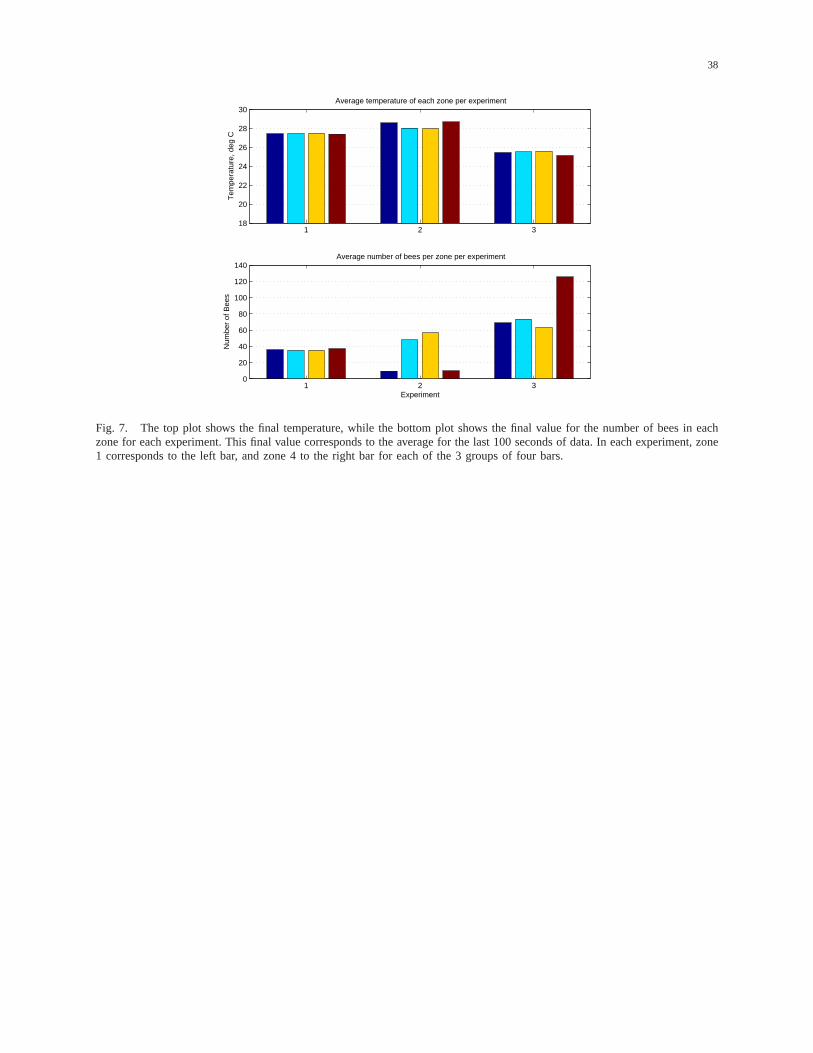
38

1 2 318

20

22

24

26

28

30Average temperature of each zone per experiment

Tem

pera

ture

, deg

C

1 2 30

20

40

60

80

100

120

140Average number of bees per zone per experiment

Experiment

Num

ber

of B

ees

Fig. 7. The top plot shows the final temperature, while the bottom plot shows the final value for the number of bees in eachzone for each experiment. This final value corresponds to the average for the last 100 seconds of data. In each experiment, zone1 corresponds to the left bar, and zone 4 to the right bar for each of the 3 groups of four bars.