Homological Algebra andAlgebraic Topology

Wojciech Chacholski & Roy Skjelnes

Lecture notes for the course SF2735. October 2009

Institutionen for matematik, KTH.

Introduction

The course is aimed for students who have had some experience with groups,and perhaps seen the definition of rings. We have tried to make these seriesof lectures self-contained. The theory is often given in terms of commutativerings, but many of the examples are given for the ring of integers. Thetheoretical result that often simplifies the situation when considering the ringof integers is the Structure Theorem for finitely generated abelian groups.Recall that a finitely generated abelian group M can be written as

M = Z/(n1)× · · · × Z/(np),

for some non-negative integers 0 ≤ n1 ≤ n2 · · · ≤ np. This provides adescription of finitely generated modules over the integers, a description weuse to give examples of the general theory and of general definitions.

The purpose of the second part of these notes concerning topological spacesis to introduce the basic concepts of topological spaces and their homologygroups. We stress examples and tools to compute these invariants. In par-ticular we compute the homology of spheres and projective spaces.

We do not claim any originality with the text. We have freely used theexisting literature as reference. In particular, for the first six chapters we diduse Rotman, “Introduction to Homological Algebra” as guidance. That bookwas in particular useful for the technical proofs dealing with resolutions andthe independence of the choices involved.

ii

Contents

1 Modules 1

1.1 Rings . . . . . . . . . . . . . . . . . . . . . . . . . . . . . . . . 1

1.2 Modules . . . . . . . . . . . . . . . . . . . . . . . . . . . . . . 2

1.3 Submodules and quotients . . . . . . . . . . . . . . . . . . . . 3

1.4 Basis . . . . . . . . . . . . . . . . . . . . . . . . . . . . . . . . 3

1.5 Direct sum . . . . . . . . . . . . . . . . . . . . . . . . . . . . . 5

1.6 Homomorphisms . . . . . . . . . . . . . . . . . . . . . . . . . 6

1.7 Determinants . . . . . . . . . . . . . . . . . . . . . . . . . . . 10

1.8 Exercises . . . . . . . . . . . . . . . . . . . . . . . . . . . . . . 11

2 Complexes 14

2.1 Complexes . . . . . . . . . . . . . . . . . . . . . . . . . . . . . 14

2.2 Chain maps . . . . . . . . . . . . . . . . . . . . . . . . . . . . 16

2.3 Exercises . . . . . . . . . . . . . . . . . . . . . . . . . . . . . . 18

3 Hom-functors 20

3.1 The Hom-functors . . . . . . . . . . . . . . . . . . . . . . . . . 20

3.2 Projective modules . . . . . . . . . . . . . . . . . . . . . . . . 21

3.3 Injective modules . . . . . . . . . . . . . . . . . . . . . . . . . 23

3.4 Exercises . . . . . . . . . . . . . . . . . . . . . . . . . . . . . . 26

4 Homology 28

4.1 Homology . . . . . . . . . . . . . . . . . . . . . . . . . . . . . 28

4.2 Homotopy . . . . . . . . . . . . . . . . . . . . . . . . . . . . . 31

4.3 Exercises . . . . . . . . . . . . . . . . . . . . . . . . . . . . . . 32

iii

5 Resolutions and Ext 34

5.1 Free resolutions . . . . . . . . . . . . . . . . . . . . . . . . . . 34

5.2 Finite resolutions . . . . . . . . . . . . . . . . . . . . . . . . . 35

5.3 Projective resolutions . . . . . . . . . . . . . . . . . . . . . . . 36

5.4 Injective resolutions . . . . . . . . . . . . . . . . . . . . . . . . 42

5.5 Exercises . . . . . . . . . . . . . . . . . . . . . . . . . . . . . . 44

6 Tensor product and Tor 47

6.1 The construction of the tensor product . . . . . . . . . . . . . 47

6.2 Universal property of the tensor product . . . . . . . . . . . . 49

6.3 Right exactness of tensor product . . . . . . . . . . . . . . . . 50

6.4 Flat modules . . . . . . . . . . . . . . . . . . . . . . . . . . . 53

6.5 Tor . . . . . . . . . . . . . . . . . . . . . . . . . . . . . . . . . 56

6.6 Universal Coefficient Theorem . . . . . . . . . . . . . . . . . . 58

6.7 Exercises . . . . . . . . . . . . . . . . . . . . . . . . . . . . . . 59

7 Topological spaces 61

7.1 Topological spaces and continuous maps . . . . . . . . . . . . 61

7.2 Subspaces . . . . . . . . . . . . . . . . . . . . . . . . . . . . . 63

7.3 Disjoint unions . . . . . . . . . . . . . . . . . . . . . . . . . . 63

7.4 Products . . . . . . . . . . . . . . . . . . . . . . . . . . . . . . 64

7.5 Quotients . . . . . . . . . . . . . . . . . . . . . . . . . . . . . 64

7.6 Compact spaces . . . . . . . . . . . . . . . . . . . . . . . . . . 65

7.7 Euclidean spaces . . . . . . . . . . . . . . . . . . . . . . . . . 67

7.8 Simplicial operators . . . . . . . . . . . . . . . . . . . . . . . . 69

7.9 Cell attachments . . . . . . . . . . . . . . . . . . . . . . . . . 70

7.10 Real projective spaces . . . . . . . . . . . . . . . . . . . . . . 72

7.11 Topological manifolds . . . . . . . . . . . . . . . . . . . . . . . 73

7.12 Homotopy relation . . . . . . . . . . . . . . . . . . . . . . . . 74

7.13 π0(X) . . . . . . . . . . . . . . . . . . . . . . . . . . . . . . . 77

8 Homology 79

8.1 Singular homology . . . . . . . . . . . . . . . . . . . . . . . . 79

8.2 Homology and maps . . . . . . . . . . . . . . . . . . . . . . . 83

8.3 Reduced homology . . . . . . . . . . . . . . . . . . . . . . . . 84

iv

8.4 H0(X,G) . . . . . . . . . . . . . . . . . . . . . . . . . . . . . 86

8.5 Homology and homotopy . . . . . . . . . . . . . . . . . . . . . 88

8.6 Small singular simplices . . . . . . . . . . . . . . . . . . . . . 91

8.7 Reduced small singular simplices . . . . . . . . . . . . . . . . 92

8.8 Homology of spheres . . . . . . . . . . . . . . . . . . . . . . . 96

8.9 Some geometric applications . . . . . . . . . . . . . . . . . . . 97

8.10 The homology of the antipodal map . . . . . . . . . . . . . . . 99

8.11 The effect on homology of a cell attachment . . . . . . . . . . 100

8.12 The integral homology groups of the projective spaces . . . . . 102

8.13 Homology of projective spaces . . . . . . . . . . . . . . . . . . 108

v

Chapter 1

Modules

1.1 Rings

Groups considered here are abelian and denoted as (A,+) where 0 denotesthe identity element. A ring A will in these notes always mean a commutativeunital ring. Recall that a ring A is an abelian group (A,+) with an additionalproduct structure which is compatible with the group structure. The productis denoted with ·, but is in many cases simply suppressed. In any case it isa map of sets

A× A −→ A

which is associative, a·(b·c) = (a·b)·c, and distributive, a·(b+c) = a·b+a·c,for all elements a, b and c in A. The ring being commutative means thata · b = b · a, for all a, b in A. Unital means that there exists an element 1 inA such that 1 · a = a for all a.

The typical examples of rings will for us be the integers A = Z with the usualaddition and multiplication, and fields.

1.1.1 Definition. A commutative, non-zero, and unital ring A is a field ifany non-zero element a ∈ A has a multiplicative inverse a−1 in A, that is anelement such that a · a−1 = 1.

Examples of fields are the rational numbers Q, the real numbers R andthe complex numbers C. Other fields we have in mind are finite fields Fp

obtained as quotients of Z by the subgroup generated by some prime numberp.

Even though our statements usually are given in terms of general commuta-tive rings, we have our focus on the ring of integers Z and fields, only.

1

1.2 Modules

1.2.1 Definition. Let A be a ring and (M,+) an abelian group. Assumefurthermore that we have a map of sets A×M −→M, (a, x) 7→ ax, such that

a(x+ y) = ax+ ay (a+ b)x = ax+ bx

(ab)x = a(bx) 1x = x

for all elements a, b in A, and all elements x, y in M . Such a map gives theabelian group (M,+) an A-module structure. We will refer to such a map bysaying that M is an A-module.

1.2.2 Example. Any abelian group (M,+) is in a natural way a Z-module.We have the natural map

Z×M −→M

sending (n, x) to n · x = x + · · · + x. This defines a Z-module structure.Consequently, each abelian group has a natural Z-module structure.

1.2.3 Example. Let A be a field. In that case a module M over A is avector space, and the map defining the A-module structure on the abeliangroup is the usual scalar multiplication. Thus, the notion of a module is ageneralization of vector spaces.

1.2.4 Example. Let (A,+) be the abelian group structure of the ring A.Together with the product structure on A we have that A is an A-module. Infact, any ideal I ⊆ A is an A-module. Recall that a subgroup (I,+) ⊆ (A,+)such that ax ∈ I, for any a ∈ A and any x ∈ I, is called an ideal. Thus, forany ideal I ⊆ A we have that the product structure from the ring gives amap

A× I −→ I,

satisfying the criteria of (1.2.1). Hence, we have that any ideal is in a naturalway an A-module. From an ideal I in a commutative ring we can alwaysconstruct the quotient ring A/I. The quotient ring is also in a natural wayan A-module.

1.2.5 Example. Let ϕ : A −→ B be a homomorphism of rings, that is a mapof the underlying sets such that ϕ(a + b) = ϕ(a) + ϕ(b), ϕ(ab) = ϕ(a)ϕ(b)and where ϕ(1) = 1. Then the ring B can be viewed as an A-module in theobvious way. More generally, let M be a B-module. Then we have a naturalmap

A×M −→M

taking (a, x) to ϕ(a)x. It is straightforward to check that the map gives Mthe structure of an A-module. We say that the B-module M becomes anA-module by restriction of scalars.

2

1.3 Submodules and quotients

1.3.1 Definition. Let M be an A-module, and let (N,+) ⊆ (M,+) be asubgroup. If the A-module structure on M restricts to an A-module structureon N , that is, we get by restriction an induced map

A×N −→ N,

then we say that N is a submodule of M .

Note that a non-empty subset N ⊆ M which is closed under addition, andunder multiplication by elements from A, will be a submodule.

1.3.2 Lemma. Let N be a submodule of M . Then the quotient group(M/N,+) has an induced A-module structure

A×M/N −→M/N

sending (a, x) to ax, where z denotes the equivalence class of z in M/N , forz ∈M .

Proof. Let us first show that the description above indeed gives a well-definedmap. Let x and y be two elements in M that represent the same equivalenceclass in M/N . We need to see that the equivalence classes of ax and ay areequal, for any a ∈ A. Since x and y represent the same equivalence class inM/N we have that x = y + n in M for some n ∈ N . Then ax = ay + an inM , and an is in N . It follows that ax = ay in M/N . Thus there is a well-defined map, and it is readily checked that it defines an A-module structureon M/N .

1.4 Basis

Let x1, . . . , xm be m elements in an A-module M . Consider the subset

< x1, . . . , xm >= {a1x1 + . . .+ amxm | ai ∈ A} ⊆M.

1.4.1 Lemma. The set < x1, . . . , xm > is an A-submodule of M .

Proof. The set is closed under addition and also under multiplication byelements from A. Namely, if x ∈< x1, . . . , xm >, then we have that there arescalars a1, . . . , am in A such that

x = a1x1 + · · ·+ amxm.

3

For any scalar a ∈ A we have (1.2.1)

ax = aa1x+ · · ·+ aamxm,

hence the set is a submodule of M .

We refer to this as the submodule generated by the elements x1, . . . , xm. Ifthe submodule generated by x1, . . . , xm equals the ambient module M , thenwe say that x1, . . . , xm span the A-module M .

1.4.2 Definition. Let M be an A-module. If there exists a finite set ofelements x1, . . . , xm in M that spans the module, then we say that the moduleM is finitely generated.

1.4.3 Example. The integer plane M = Z × Z is a finitely generated Z-module. A set of generators is x1 = (1, 0), x2 = (0, 1). Indeed, any element(m,n) in M can be written as the sum

(m,n) = mx1 + nx2.

Hence the two elements x1 and x2 span M .

1.4.4 Example. The Fundamental Theorem for finitely generated Abeliangroups says that an abelian group is finitely generated if and only if it is ofthe form

M = Z× · · · × Z× Z/(n1)× · · · × Z/(nr),

where ni ≥ 1. Thus a finitely generated abelian group contains a finitenumber of copies of Z, and a torsion part which is the product of a finitenumber of cyclic groups of finite order. If we let xi = (0, 0, . . . , 0, 1, 0, . . . , 0) ∈M denote the element having the class of 1 at the i’th component, then theseelements span the module M .

Linear Independence

We say that the elements x1, . . . , xm in a module M are linearly independent,over A, if

m∑i=1

aixi = 0⇒ {ai = 0, for all i = 1, . . . ,m.}

Finally, we say that the ordered sequence x1, . . . , xm form an A-module basisof M if the elements span M and are linearly independent. Note that ifx1, . . . , xm is an ordered sequence that form an A-module basis of M , thenany reordering of the basis will still be linearly independent and still spanM . However, generally a reordering of a basis will give a different basis.

4

1.4.5 Definition. A module M that admits a basis is called a free module.

1.4.6 Remark. The zero module M = 0 is a free module. The basis is theempty set.

1.4.7 Example. The elements x1 and x2 of Example (1.4.3) will form a basis.

1.4.8 Example. One major difference between modules and vector spaces isthat modules do not always have a basis. For instance, the field F2 of twoelements is a quotient of Z, and in particular a Z-module. The element1 ∈ F2 spans the module, whereas the zero element does not. The element 1is however not a basis, as for instance 0 · 1 = 2 · 1 in F2.

1.4.9 Example. The elements {x1, . . . , xn} of the Example (1.4.4) will in ingeneral not form a basis. In fact it will be a basis if and only if the grouphas no torsion part.

1.4.10 Proposition. Let M be an A-module that admits a basis x1, . . . , xm.Then the any other basis of M will have the same number of elements.

Proof. Exercise (1.8.11).

1.4.11 Definition. An A-module M which has a basis consisting of m ele-ments is said to be free of rank m.

1.4.12 Example. For vector spaces we have that any non-zero element canbe extended to be part of some basis. This is not true for modules, not evenwhen the module does have a basis. Consider the ring of integers Z as amodule over itself. The element 1 will form a basis, as well as the element-1. However, any other non-zero element x will be linearly independent, butthe element will not span Z. For instance, in the free rank one module Z wehave the descending chain of proper submodules Z ⊃ (2) ⊃ (4) ⊃ (8) · · ·

1.5 Direct sum

Let {Mi}i∈I be a collection of A-modules, indexed by some set I. The product×i∈IMi consisting of all sequences of elements (xi)i∈I with xi ∈ Mi is anabelian group by componentwise addition. The product becomes naturallyalso an A-module via

(a, (xi)i∈I) 7→ (axi)i∈I ,

for all a ∈ A, and all sequences (xi)i∈I in the product.

5

1.5.1 Definition. Let A be a ring, and let {Mi}i∈I be a collection of A-modules. The direct sum ⊕i∈IMi is defined as the A-submodule

⊕i∈IMi ⊆ ×i∈IMi

consisting of sequences (xi) where all but a finite number of elements arezero.

1.5.2 Remark. Note that in general the direct sum is a proper submodule ofthe product. However, when the indexing set I is finite, then the direct sumequals the product.

1.5.3 Example. It is interesting to consider the direct sum of copies of A,that is Mi = A for i = 1, . . . , n. The module M = ⊕ni=1A contains the nelements

ei := (0, 0, . . . , 0, 1, 0, . . . , 0),

where 1 appears on the i’th component for i = 1, . . . , n. From the definitionof the module M = ⊕ni=1A we have that any element x ∈ M is of the formx = (x1, . . . , xn), with xi ∈ A. We can therefore write

x = (x1, . . . , xn) = x1e1 + · · ·+ xnen.

Thus any element x ∈M is anA-linear combination of the elements e1, . . . , en,and moreover the linear combination is unique. The elements e1, . . . , en forman A-module basis of M . In particular the ring A viewed as a module overitself has the basis 1.

1.6 Homomorphisms

Having defined the notion of an A-module, we will need to define the notionof maps between these objects.

1.6.1 Definition. Let M and N be two A-modules. An A-module homo-morphism is a map of the underlying sets f : M −→ N , such that

f(ax+ by) = af(x) + bf(y)

for all a, b in A, and all x, y in M .

Note that an A-module homomorphism f : M −→ N is exactly the same asa group homomorphism that is compatible with the A-module structure.

6

Kernel and Image

The kernel of an A-module homomorphism f : M −→ N is the set

Ker(f) = {x ∈M | f(x) = 0}.

Any module has the zero element 0 ∈ M , and the zero element is in thekernel of any A-module homomorphism. An A-module homomorphism f issaid to be injective if the kernel is trivial, that is Ker(f) = 0. The image isthe set

Im(f) = {f(x) | x ∈M} ⊆ N.

The homomorphism is surjective if the image equals all of N . An A-modulehomomorphism f : M → N is an isomorphism if both injective and surjective.

1.6.2 Lemma. An A-module M is free if and only if it is isomorphic to⊕i∈IA, for some (possibly empty) indexing set I.

Proof. See Exercise (1.8.19).

1.6.3 Lemma. Let f : M −→ N be an A-module homomorphism. Then wehave the following.

(1) The kernel Ker(f) is an A-submodule of M .

(2) The image Im(f) is an A-submodule of N .

(3) The homomorphism f has a unique factorization through an injectiveA-module homomorphism f : M/Ker(f) −→ N .

In particular we have that if f : M −→ N is a surjective A-module homo-morphism, then f : M/Ker(f) −→ N is an isomorphism.

Proof. Readily checked.

For any A-module M we have the identity morphism idM : M −→M sendingx to x, for all x ∈M .

1.6.4 Lemma. Let f : M −→ N be an A-module isomorphism. Then thereexists a unique A-module homomorphism g : N −→ M such that gf = idMand fg = idN .

Proof. There is a set-theoretic map g : N −→ M having the property thatg(f(x)) = x and f(g(y)) = y for all x ∈ M , all y ∈ N . One has to verifythat this map is in fact an A-module homomorphism.

7

1.6.5 Proposition. A module M is finitely generated if and only if themodule can be written as a quotient module of a free module of finite rank.

Proof. Note that the image of an A-module homomorphism f : ⊕mi=1A −→Mis exactly the same as the submodule generated by f(e1), . . . , f(em). Thus,m elements in M that span the module M is exactly the same as having asurjective map f : ⊕mi=1 A −→M .

The set of all A-module homomorphisms from an A-module M to anotherA-module N is denoted

HomA(M,N).

If M = N then a homomorphism is referred to as an endomorphism, and theset of all endomorphisms is denoted as EndA(M).

1.6.6 Lemma. Let M and N be two A-modules. The set HomA(M,N)becomes an abelian group with pointwise addition, and has the structure ofan A-module by the map

A× HomA(M,N) −→ HomA(M,N)

sending (a, f) to the map M −→ N that takes x to af(x).

Proof. Readily checked.

1.6.7 Proposition. Let M1, . . . ,Mn be A-modules, and let M = ⊕ni=1Mi

denote their direct sum. For any A-module N we have a natural isomorphism

HomA(⊕ni=1Mi, N) = ⊕ni=1HomA(Mi, N).

Thus, giving an A-module homomorphism from a finite direct sum is equiv-alent to giving A-module homomorphisms from the components appearing inthe direct sum.

Proof. There is an A-module map ck : Mk −→M = ⊕ni=1Mi sending elementsx 7→ (0, 0, . . . , 0, x, 0, . . . , 0) to the k’th component, for k = 1, . . . , n. Anymorphism f : M −→ N composed with ck give an A-module homomorphismf ◦ ck : Mk −→ N . We then get an A-module homomorphism

Φ: HomA(M,N) −→ ⊕ni=1HomA(Mi, N) (1.1)

taking f 7→ (f ◦ c1, . . . , f ◦ cn). Let us now construct the morphism going theother way. Let (f1, . . . , fn) be an element of ⊕ni=1HomA(Mi, N). Then each

8

fk is an A-module homomorphism Mk −→ N , and we define the A-modulehomomorphism f : M −→ N by

f(x1, . . . , xn) := f1(x1) + · · ·+ fn(xn).

One checks that since each fk is an A-module homomorphism, then alsothe map f is an A-module homomorphism. We have then constructed anA-module homomorphism Ψ which we need to check is the inverse of (1.1).Let f : M −→ N be an A-module morphism, and consider the A-modulehomomorphism Ψ(Φ(f)) : M −→ N . We want to show that these two ho-momorphisms are equal, which means that they have exactly the same valueon every element x ∈M . We have that

Ψ(Φ(f))(x) = Ψ(f ◦ c1(x), . . . , f ◦ cn(x)) = f ◦ c1(x) + · · ·+ f ◦ cn(x).

As x ∈M we have that x = (x1, . . . , xn), with xk ∈Mk, for all k = 1, . . . , n.Consequently, we have that

f ◦ c1(x) + · · ·+ f ◦ cn(x) = f(x1, 0, . . . , 0) + · · ·+ f(0, . . . , 0, xn)

= f(x1, . . . , xn) = f(x).

Hence Ψ(Φ) is the identity. One checks in a similar way that Φ(Ψ) also equalsthe identity, and thereby completes the proof of the proposition.

1.6.8 Corollary. Let M be an A-module with basis e1, . . . , em and N an A-module with basis f1, . . . , fn. Then the A-module HomA(M,N) is isomorphicto the A-module of (n×m)-matrices with coefficients in A.

Proof. As M has basis e1, . . . , em we can by Lemma (1.6.2) identify M with⊕mi=1A. Consequently, by the proposition, we have

HomA(M,N) = ⊕mi=1HomA(A,N).

Any A-module homomorphism f : A −→ N is determined by its value onthe element 1 ∈ A, and moreover any element in N would give rise to anA-module homomorphism. It follows that HomA(A,N) = N . As N has basisf1, . . . , fn we have thatN = ⊕ni=1A. Consequently HomA(A,N) equals the A-module of ordered n-tuples of elements in A, and we have that HomA(M,N)equals the A-module of ordered m · n-tuples of elements in A. This is thesame as (n×m)-matrices with coefficients in A.

9

Matrix notation

It is customary to represent an A-module homomorphism f : ⊕mi=1 A −→⊕ni=1A with an (n ×m) matrix Xf where the k’th column is the coefficientof f(0, . . . , 0, 1, 0, . . . , 0). An element x ∈ ⊕mi=1A is then viewed as a columnvector [x] := [x1, . . . , xm]tr, and the action of f on this particular element isthen given by the matrix multiplication Xf · [x].

1.7 Determinants

Consider now the situation with an A-module M that has a basis e1, . . . , em.Let f : M −→ M be an endomorphism, which we can by (1.6.8) representuniquely with an (m×m)-matrix

Xf =

a1,1 a1,2 · · · a1,m

a2,1 a2,2...

.... . .

...am,1 am,2 . . . am,m

,with coefficients ai,j ∈ A. We define the determinant of the endomorphismf : M −→M to be the determinant of the corresponding matrix representa-tion,

det(f) :=∑σ∈Sm

(−1)|σ|a1,σ(1) · · · am,σ(m).

Note that det(f) is an element of the ring A.

1.7.1 Proposition. Let f : M −→M be an A-module endomorphism of anA-module that has a finite basis. Then f is an isomorphism if and only ifdet(f) is invertible in A.

Proof. If f were an isomorphism it would be invertible. On the level ofmatrices there would exist a matrix Y such that the product XfY wouldequal the identity matrix Im. The determinant of the identity matrix is 1,and we would get

1 = det(XfY ) = det(f) · det(Y ) ∈ A.

In other words det(f) is invertible in A. To prove the converse, let ad(M) de-note the adjoint matrix of Xf . The adjoint matrix is the transpose of the co-factor matrix, where the coefficient (i, j) of the cofactor matrix is (−1)i+jci,j,with ci,j being the determinant of the matrix Xf with row i and column j

10

removed. Note that the adjoint matrix has coefficients in A, and Cramer’sidentity yields the following matrix equality

Xf · ad(X) = det(f) · Im.

As det(f) was assumed invertible we get that

det(f)−1ad(X)

is the matrix inverse of Xf . Hence f : M −→ M has an inverse, and isconsequently an isomorphism.

1.8 Exercises

1.8.1. Show that the fields R and C are not isomorphic.

1.8.2. Show that the multiplicative inverse of an element x in a commutative unital ringA is unique, if it exists.

1.8.3. Solve the equation 3x = 2 in Z/(7).

1.8.4. Describe all ideals I in the ring A = Z/(12), and in each case describe the quotientring A/I.

1.8.5. The sum of two subvector spaces V1 and V2 of a vector space V is defined as

V1 + V2 = {x1 + x2 | xi ∈ V } ⊆ V.

The sum is again a vector space. Show that

dim(V1 + V2) = dim(V1) + dim(V2)− dim(V1 ∩ V2).

1.8.6. Consider an inclusion of A-modules L ⊆ N ⊆M . Show that we have the inclusionN/L ⊆M/L, and that we have

(M/L)/(N/L) = M/N.

1.8.7. Let A be a commutative unital ring. Assume that A contains no zero-divisors otherthan the zero element 0 ∈ A, and assume that the underlying set |A| is finite. Show thatA is in fact a field. (An element x ∈ A is a zero-divisor if there exists a non-zero elementy such that xy = 0).

1.8.8. Let ϕ : A −→ B be a homomorphism of rings.

(1) Show that if J ⊆ B is an ideal, then ϕ−1(J) is an ideal in A.

(2) Let I ⊆ A be an ideal. Show that if ϕ is surjective, then ϕ(I) is an ideal in B.

(3) Show, by an example, that ϕ(I) is not necessary an ideal, even if I is an ideal.

1.8.9. Verify that a0 = 0 and that (a − b)x = ax − bx for any elements a, b in a ring A,and any x in an A-module M .

11

1.8.10. Let V be a vector space over some field F , and let F [X] denote the polynomialring in one variable X over F . Show that a F [X]-module structure on V is equivalentwith having a F -linear map T : V −→ V .

1.8.11. Let E be a free A-module that admits a basis β = e1, . . . , en. Show that any otherbasis of E will have the same cardinality as β.

1.8.12. Let E be a free A-module of finite rank. Show that EndA(E) is free A-module,and find a basis.

1.8.13. Let M be an A-module, and let M∗ = HomA(M,A) denote its dual. Show thatthere is a natural A-module homomorphism M −→ (M∗)∗ from a module to its doubledual. Show, furthermore, that if M is free of finite rank, then M is isomorphic to itsdouble dual.

1.8.14. Let M be an A-module. Show that the A-module EndA(M) has a ring (notnecessarily commutative) structure by composition.

1.8.15. A non-zero A-module M is called simple if the only submodules are the zeromodule and M itself. Thus a module M is simple if the trivial submodules are the onlysubmodules of M .

(1) Show that a simple module is isomorphic to A/m for some maximal ideal m in A.

(2) Show Schur’s Lemma: Let f : M −→ N be an A-module homomorphism betweentwo simple modules. Show that f is either the zero map or an isomorphism.

(3) Show that if M is simple, then EndA(M) is a skew-field; that is, a not necessarilycommutative field.

1.8.16. The sum of two submodules M and N of an A-module P is defined similarily aswith vector spaces (1.8.5). Show that

(M +N)/N = N/(M ∩N).

1.8.17. Let M be an A-module, and I ⊆ A an ideal generated by x1, . . . , xn. Assume thatfor each i = 1, . . . , n there exists an integer pi such that xpi

i annihilates M . Show thatthere exists an integer m such that Im annihilates M . (An element a ∈ A annihilatesan element m ∈ M if am = 0, and the element a ∈ A annihilates M if am = 0 for allm ∈M).

1.8.18. Let I ⊆ A be a non-zero ideal. Show that I is a free A-module if and only if I isprincipally generated by an element which is not a zero-divisor. (An ideal I is principallygenerated if it is generated by one element).

1.8.19. Prove Lemma (1.6.2).

1.8.20. Show that the Z-submodule Z[p] ⊆ Q consisting of all integer coefficient polyno-mial expressions in p, is not finitely generated unless p ∈ Z.

1.8.21. An element x in an A-module M is a torsion element if there exists an elementa ∈ A that is not a zero-divisor and annihilates x (1.8.17). Show that the torsion elementsin M form an A-submodule, the torsion module of M .

1.8.22. Show that Q is torsion free, but not free as an Z-module.

1.8.23. Show that HomZ(Z/(m),Z) = 0 for any non-zero integer m 6= 0.

12

1.8.24. Show that HomZ(Z/(m),Z/(n)) = Z/(d), where d is the greatest common divisorof m and n.

1.8.25. Let

M =[1 1 −10 2 3

],

where the coefficients in the matrix are in Z/(30). Show that the rows of M are linearlyindependent over Z/(30), but any two columns are linearly dependent (a situation whichdoes not occur for vector spaces).

1.8.26. The integer plane Z2 consists of all ordered pairs of integers v = (n,m). We haveseen (Example (1.4.7)) that the integer plane is a free Z-module of rank two.

1. Let v = (m,n) be a vector in the integer plane Z2. Show that v is part of a basisif and only if (m,n) = 1 (the integers are coprime).

2. Let v = (5, 12). Extend u to a basis of the integer plane.

1.8.27. Show that Z/(m)⊕ Z/(n) = Z/(nm) if and only if (n,m) = 1.

1.8.28. Find an example where M ⊕ P = N ⊕ P , but where M is not isomorphic to N .

1.8.29. A ring A is noetherian if any ascending chain of ideals I1 ⊆ I2 ⊆ · · · becomesstationary. Show that the ascending chain condition is equivalent with any submodule ofa finitely generated module being finitely generated. In particular any ideal in a noetherianring is finitely generated. As the ideals in Z are principally generated, we have that Z isa noetherian ring.

13

Chapter 2

Complexes

2.1 Complexes

Let P• = {Pn, dn}n∈Z be a family of modules Pn, and module homomorphisms

dn : Pn −→ Pn−1

indexed by the integers. The module Pn is the degree n component of thefamily, and the homomorphism dn is the boundary operator in degree n. Notethat the boundary operators are decreasing the degree. We will eventuallyalso allow these boundary operators to be increasing, but as default we con-sider decreasing boundary operators.

A collection {Pn, dn} with decreasing boundary operators is called a complexif dn−1◦dn = 0, for all n. And a collection {Pn, dn} with increasing boundaryoperators is called a complex if dn+1 ◦ dn = 0, for all n.

The issue with ascending versus descending boundary operators is a matter ofindexing, the important property is that the composition of any two adjacentboundary operators equals the zero map.

2.1.1 Lemma. The composition of two module homomorphisms f : M −→N and g : N −→ P is the zero homomorphism if and only if

Im(f) ⊆ Ker(g).

In particular, a family {Pn, dn} of modules a homomorphisms, is a complexif and only if

Im(dn+1) ⊆ Ker(dn),

for all n.

14

Proof. This is just a restatement.

2.1.2 Example. Any module M can be viewed as a complex

· · · −→ 0 −→ · · · −→ 0 −→M −→ 0 −→ · · · .

It is customary to put the module M in degree zero, unless otherwise men-tioned. So M is the complex {Pn, dn} where P0 = M , and all the other arezero modules. The boundary operators dn are all the zero map.

2.1.3 Example. The sequence of Z-modules

· · · // 0 // Z4 // Z // Z/(2) // 0 // · · ·

is a complex. The first non-trivial map is multiplication by 4, and the secondnon-trivial map is the quotient map. The multiplication by a non-zero integern : Z −→ Z is always injective, and the image of such a map is the submodule(n) ⊆ Z generated by n. The kernel of the projection morphism Z −→ Z/2is the submodule (2). We then have that in the sequence above we couldhave replaced 4 with any integer of the form 2n, and the sequence would stillbe a complex.

2.1.4 Remark. Strictly speaking a complex is indexed by the integers, butoften we encounter a finite collection of modules and homomorphism. Wewill in such cases tacitly assume that the other modules are zero modules. Inparticular if we have a sequence of A-modules and A-module homomorphisms

Pndn // · · · dk // Pk−1 ,

where Im(dp) ⊆ Ker(dp−1) for all n ≤ p < k, we will refer to the sequencebeing a complex. This means that we assume that Pm = 0 for m ≥ n andfor m ≤ k − 2.

2.1.5 Definition. A complex {Pn, dn} is an exact sequence if Im(dn+1) =Ker(dn) for all n. Furthermore, an exact sequence with at most three non-trivial elements is a short exact sequence, and written as

0 −→M −→ N −→ P −→ 0.

2.1.6 Example. The complex (2.1.3) is not exact, but

0 // Z4 // Z // Z/(4) // 0

is short exact.

15

2.1.7 Example. Let f : M −→ N be an A-module homomorphism. Thecokernel of a homomorphism f is the quotient module N/Im(f), and usuallydenoted Coker(f). We can then form the sequence

0 // Ker(f) //Mf // N // Coker(f) // 0

which we consider being an complex with other terms being zero modulesand suppressed, and where the degrees also are suppressed. The complex isexact by construction.

2.1.8 Example. Note that a sequence Mf // N // 0 is exact is equivalent

with f being surjective. A sequence 0 //Mf // N is exact is equivalent

with f being injective. Exactness of the sequence

0 //Mf // N // 0

is another way of saying that f is an isomorphism.

2.2 Chain maps

Consider the diagram

Mf //

d��

M ′

d′

��N

g // N ′

of A-modules and A-module homomorphisms. Such a diagram is referred toas being commutative if d′ ◦ f = g ◦ d.

2.2.1 Definition. A chain map f : P• −→ Q• is a collection of A-modulehomomorphisms fn : Pn −→ Qn commuting with the boundary operators. Inother words we have commutative diagrams

Pnfn //

dPn��

Qn

dQn��

Pn−1fn−1 // Qn−1

for every n.

16

2.2.2 Example. Consider the diagram

0

��

// Z4 //

��

Z

��

// 0

��0 // 0 // Z/(2) // 0.

Each horizontal row we think of representing a complex. As the diagramscommute we have that the diagram represents a chain map of complexes.

2.2.3 Proposition (Snake Lemma). Let

M1

f1��

ϕ1 //M2

f2��

ϕ2 //M3

f3��

// 0

0 // N1ψ1 // N2

ψ2 // N3

be a commutative diagram of A-modules and A-module homomorphisms,where the two horizontal sequences are exact. Then we have a long exactsequence of A-modules

Ker(f1) // Ker(f2) // Ker(f3)

δgggggggggggg

ssggggggggggg

Coker(f1) // Coker(f2) // Coker(f3)

. (2.1)

The two first and the two last homomorphisms are the obvious ones, whereasthe connecting homomorphism δ takes an element x ∈ Ker(f3) to the class of

ψ−11 (f2(ϕ

−12 (x))) ∈ Coker(f1).

Furthermore, if ϕ1 is injective, then the left most homomorphism in the longexact sequence is injective. If ψ2 is surjective, then the rightmost homomor-phism in the long exact sequence is surjective.

Proof. It is readily checked that we have an induced homomorphism of ker-nels and cokernels, that is the two first and the two last arrows of the se-quence displayed above. We will describe the particular map δ : Ker(f3) −→coker(f1). Let x ∈M3 be an element mapped to zero by f3, and let x′ ∈M2

be any element such that ϕ2(x′) = x. By commutativity of the diagram we

have ψ2(f2(x′)) = f3(x), hence f2(x

′) ∈ Ker(ψ2). Consequently there is aunique element x′′ ∈ N1 such that ψ1(x

′′) = f2(x′). Let δ(x) be the image of

x′′ by the quotient map N1 −→ coker(f1). This prescribed map involved a

17

choice of pre-image x′ of x, and we need to check that we indeed get a well-defined map. Let y′ ∈ M2 be another pre-image of x. Then ϕ2(x

′ − y′) = 0.By exactness of the upper row there exist z ∈M1 such that ϕ1(z) = x′ − y′.By the commutativity of the left diagram it follows that the two differentpre-images x′ and y′ give the same element in coker(f1). Consequently wehave a well-defined map δ : Ker(f3) −→ coker(f1), which is easily seen to bean A-module homomorphism.

We furthermore leave to the reader to check that we not only have obtaineda complex in (2.1), but that it is actually an exact sequence. The only partwe will go through in detail is exactness at one particular step. We will showthat Ker(δ) equals the image of the induced map Ker(f2) −→ Ker(f3). Sincewe assume that the reader has verified that we have a complex we need onlyto show that any element in the kernel of δ is the image of some elementin Ker(f2). Let x be an element of Ker(f3) which is mapped to zero by δ,that is x ∈ ker(δ). We need show that there exists an x′ ∈ Ker(f2) such thatϕ2(x

′) = x. Let x′ ∈M2 be any pre-image of x, and let y ∈ N1 be the elementsuch that ψ1(y) = f2(x

′). Then we have that δ(x) is the image of y by thequotient map N1 −→ coker(f1). We have assumed that δ(x) = 0, whichthen means that y = f1(z), for some z ∈ M1. Now consider the elementx′ − ϕ1(z) ∈M2, which is a pre-image of x, as

ϕ2(x′ − ϕ1(z)) = ϕ2(x

′)− ϕ2(ϕ1(z)) = x− 0.

Using the commutativity of the left diagram we obtain that

f2(x′ − ϕ1(z)) = f2(x

′)− f2(ϕ1(z)) = f2(x′)− ψ(f1(z)).

As f1(z) = y and ψ1(y) = f2(x′), we get that f2(x

′−ϕ1(z)) = 0. We thereforehave an element x′−ϕ1(z) in the kernel of f2 which is mapped to the elementx. Consequently Ker(δ) equals the image of Ker(f2).

2.3 Exercises

2.3.1. Let N1 and N2 be two submodules of M . Show that we have a short exact sequence

0 −→ N1 ∩N2 −→ N1 ⊕N2 −→ N1 +N2 −→ 0,

where the first map sends x to (x, x), and the second map takes (x, y) to x− y.

2.3.2. Let f : M −→ N and g : N −→ P be two A-module homomorphisms. Show thatthere is an exact sequence

0→ Ker(f)→ Ker(gf)→ Ker(g)→ Coker(f)→ Coker(gf)→ Coker(g)→ 0.

18

2.3.3. Given a short exact sequence 0→M → N → P → 0, and given f : P ′ → P . Showthat there exist a commutative diagram and exact rows of the form

0 // M //

��

N ′

��

// P ′

f

��

// 0

0 // M // N // P // 0

2.3.4. Given chain maps f : P• −→ Q• and q : Q• −→ R• that, for every n, form thecommutative diagrams and exact sequences of A-modules

0 // Pnfn //

dPn

��

Qn

dQn

��

gn // Rn //

dRn

��

0

0 // Pn−1fn−1 // Qn−1

gn−1 // Rn−1// 0.

Show that we obtain induced commutative diagrams and exact sequences

Coker(dPn+1)

��

// Coker(dQn+1) //

��

Coker(dRn+1) //

��

0

0 // Ker(dPn−1) // Ker(dQn−1) // Ker(dRn−1)

2.3.5. Let0 −→ Fn −→ Fn−1 −→ · · · −→ F0 −→ 0

be an exact sequence of finitely generated free A-modules Fi. Show that

n∑i=0

(−1)irank(Fi) = 0.

19

Chapter 3

Hom-functors

3.1 The Hom-functors

Let M be an A-module. We have, for any A-module N , that the set ofA-module homomorphisms from M to N , HomA(M,N), form an A-module.Note that if f : N1 −→ N2 is an A-module homomorphism we get an inducedA-module homomorphism

f∗ : HomA(M,N1) −→ HomA(M,N2),

by composition; a homomorphism ϕ : M −→ N1 is mapped to f∗(ϕ) := f ◦ϕ.

3.1.1 Proposition. Let M be an A-module, and let

0 // N1f // N2

g // N3// 0

be a short exact sequence of A-modules. Then we get an exact sequence

0 // HomA(M,N1)f∗ // HomA(M,N2)

g∗ // HomA(M,N3).

Proof. Let ϕ : M −→ N1 be an A-module homomorphism. We have thatg∗ ◦ f∗(ϕ) is the composition of the three homomorphisms g, f and ϕ. As thecomposition of g and f is the zero map, it follows that the sequence (3.1.1)is a complex. To establish injectivity of f∗, we assume that ϕ is in the kernelof f∗. That is, the composition

Mϕ // N1

f // N2

is the zero map. If ϕ : M −→ N1 was not the zero map, there would existan x ∈ M such that ϕ(x) 6= 0. But then f∗(ϕ) would take that particular

20

element to f(ϕ(x)), which would be non-zero as f is injective. It follows thatϕ is the zero homomorphism, and f∗ is injective. Now we want to show thatIm(f∗) = Ker(g∗). As we already have seen that the sequence (3.1.1) is acomplex, we need only to show that Ker(g∗) ⊆ Im(f∗). Let ϕ : M −→ N2

be an element of the kernel of g∗. Then in particular we have g∗(ϕ(x)) = 0for every x ∈ M . As the image of f equals the kernel of g, we obtainthat the image of ϕ is contained in the image of f , that is Im(ϕ) ⊆ Im(f).Furthermore, as f is injective each element in the image has an unique pre-image in the domain. Define now the map of sets ϕ′ : M −→ N1 by takingx ∈M to the unique preimage of ϕ(x). This is not only a well-defined map,it is readily checked that in fact this is an A-module homomorphism. Byconstruction we have that f∗(ϕ

′) = ϕ, and consequently ker(g∗) = Im(f∗),and we have proven the proposition.

3.1.2 Example. Our favorite example is the short exact sequence

0 // Z2 // Z // Z/(2) // 0.

Apply now the functor HomZ(Z/(2),−) to that sequence and we obtain theexact sequence

0 // HomZ(Z/(2)),Z)2∗ // // HomZ(Z/(2),Z) // HomZ(Z/(2),Z/(2)).

By Exercise (1.8.23) we have that the module HomZ(Z/(2),Z) is the zeromodule. On the other hand we clearly have that HomZ(Z/(2),Z/(2)) 6= 0,as it contains the identity morphism. We have that the sequence consideredabove is exact, but we have just shown that the rightmost arrow is notsurjective. The sequence in question is

0 −→ 0 −→ 0 −→ HomZ(Z/(2),Z/(2)) = Z/(2).

3.2 Projective modules

The assignment taking an A-module N to the A-module HomA(M,N) isfunctorial. We say that HomA(M,−) is a left exact functor as the functortakes short exact sequences to left exact sequences. As the Example (3.1.2)above shows, the functor is not right exact, in general, since right exactnessis not preserved. One could however ask for which modules M the functorHomA(M,−) takes short exact sequences to short exact sequences. Suchmodules certainly exist, take M = 0 for instance. A functor that takes shortexact sequences to short exact sequences is called an exact functor.

21

3.2.1 Definition. An A-module P is projective if for any surjection of A-modules Q′ −→ Q, any homomorphism g : P −→ Q can be extended to ahomomorphism g′ : P −→ Q′. That is, given the diagram of A-modules,

P

g

����~~

~~

Q′ // Q // 0,

and solid arrows representing homomorphisms, with the horizontal sequenceexact. Then there exists a homomorphism, represented by the dotted arrow,making the diagram commutative.

3.2.2 Example. Any free module satisfies the defining property of a projectivemodule. Hence a free module is projective.

3.2.3 Theorem. A module P is projective if and only if HomA(P,−) is anexact functor.

Proof. Let P be a projective module. By (3.1.1) we have that HomA(P,−)is left-exact. We need only to check that it also preserves surjections. Letf : N −→ N ′ be a surjective A-module homomorphism. We need to showthat the associated A-module homomorphism

HomA(P,N)f∗ // // HomA(P,N ′) (3.1)

is surjective. Let ϕ ∈ HomA(P,N ′), and consider the diagram

Nf // N ′ // 0

P

ϕ

OO . (3.2)

The horizontal sequence is exact, and by definition of projectivity there existsa lifting ϕN : P −→ N of ϕ. Then we have that f∗(ϕN) = ϕ, and thehomomorphism (3.1) is surjective. Conversely, assume that HomA(P,−) isan exact functor. In particular that means that for any surjection f : N −→N ′, and any diagram as (3.2), there would exist a lifting since the modulehomomorphism (3.1) is surjective. In other words P is projective.

22

3.3 Injective modules

We now consider the dual situation, fixing N instead of M when consideringHomA(M,N). If f : M1 −→ M2 is an A-module homomorphism we get aninduced A-module homomorphism

f ∗ : Hom(M2, N) −→ Hom(M1, N),

given by composition ϕ 7→ ϕ ◦ f . Note that the arrows get reversed, and wesay that HomA(−, N) is a contravariant-functor.

3.3.1 Proposition. Let N be an A-module, and let

0 //M1f //M2

g //M3// 0

be a short exact sequence of A-modules. Then we have an induced exactsequence

0 // HomA(M3, N)g∗ // HomA(M2, N)

f∗ // HomA(M1, N)

of A-modules.

Proof. That we have a complex follows from the fact that g ◦ f is the zeromap. Let us first establish injectivity of g∗. Let ϕ ∈ HomA(M3, N) be suchthat g∗(ϕ) = 0. Thus ϕ ◦ g : M2 −→ N is the zero map, which is equivalentwith Ker(ϕ) ⊇ Im(g). As the homomorphism g : M2 −→ M3 is surjective,it is necessarily so that Ker(ϕ) = M3. That is, ϕ is the zero map, and wehave injectivity of g∗. To prove exactness in the middle we need to see thatKer(f ∗) ⊆ Im(g∗). Let ϕ ∈ HomA(M2, N) be such that f ∗(ϕ) = 0. Then ϕ◦fis the zero map, which means that Im(f) ⊆ Ker(ϕ). As any homomorphismfactors through its kernel (Lemma 1.6.3, Assertion (3)), we have in particularthat ϕ factors through

ϕ : M2/Im(f) = M3// N.

Then we have that g∗(ϕ) = ϕ, hence ϕ is in the image of g∗. In other wordsHomA(−, N) is left exact.

3.3.2 Example. Let us again consider our favorite example, the exact sequence

0 // Z2 // Z // Z/(2) // 0.

23

Apply HomZ(−,Z/(2)) to the sequence above, and we get the exact sequence

0 // HomZ(Z/(2),Z/(2)) // HomZ(Z,Z/(2)) 2∗ // HomZ(Z,Z/(2)).

Since Z is a free module over itself, a homomorphism Z −→ N is determinedby its action on 1. Furthermore, as such a homomorphism can send 1 toanything in N we have that HomZ(Z,Z/(2)) = Z/(2). The identification isthus to send a homomorphism f : Z −→ Z/(2) to f(1) ∈ Z/(2). Note thatunder that identification the morphism

2∗ : Z/(2) −→ Z/(2)

corresponds to multiplication by 2. In other words 2∗ is the zero homomor-phism, and we have that the sequence above is not surjective at the right.

3.3.3 Definition. An A-module I is injective if for any injective homo-morphism Q −→ Q′, we have that any homomorphism ϕ : Q −→ I can beextended to a homomorphism ϕ′ : Q′ −→ I. That is, given a diagram ofA-modules,

I

0 // Q

ϕ

OO

// Q′

__@@

@@

and solid arrows representing homomorphisms, with the horizontal sequenceexact, there exists a dotted arrow making the diagram commutative.

3.3.4 Proposition. An A-module I is injective if and only if any A-modulehomomorphism f : J −→ I, with J ⊆ A an ideal, can be extended to ahomomorphism f ′ : A −→ I.

Proof. As ideals J ⊆ A are particular cases of modules we immediatelyhave that if I is an injective module, then any homomorphism from an idealJ −→ I can be extended to a homomorphism A −→ I. We need to prove theconverse. Let I be an A-module such that any homomorphism from idealsin A can be extended to homomorphism from the ring. We shall show thatI is injective. Assume that we are given a diagram

I

0 // Q

ϕ

OO

// Q′

24

of A-modules where the sequence is exact. Let A denote the collection ofpairs {(P, φ)} where P is an A-module such that Q ⊆ P ⊆ Q′, and whereφ : P −→ I is an extension of ϕ. By Zorn’s Lemma (see Exercise (3.4.12))there exists a maximal element (P ′, φ′) of A . Note that if P ′ = Q′ then weget that I is injective, completing our proof. We therefore only need to showthat P ′ = Q′. Assume therefore that P ′ 6= Q, and in particular there existsan element x ∈ Q′ but where x /∈ P ′. Define the ideal

J = {a ∈ A | ax ∈ P ′} ⊆ A,

and the A-module homomorphism f : J −→ I by sending a to φ′(ax). Byassumption there exists an extension f ′ : A −→ I of f , and we will use thisextension to define an element (P ′′, φ′′) of A . Namely, let P ′′ denote theA-module generated by elements in P ′ and by x. Elements in P ′′ are then ofthe form p+ ax, with p ∈ P and a ∈ A. Furthermore, P ′′ is contained in Q′,and contains P ′ as a proper submodule since x /∈ P ′. Define the A-modulehomomorphism

φ′′ : P ′′ −→ I

by sending p+ax to φ′(p)+a ·f ′(1). We have by Exercise (3.4.13) that φ′′ is awell-defined A-module homomorphism. Given that, we have now constructeda pair (P ′′, φ′′) in A that violates the maximality of the pair (P ′, φ′). Henceour assumption that P ′ 6= Q′ fails and we have indeed that P ′ = Q′.

3.3.5 Proposition. An A-module I is injective if and only if the contravari-ant functor HomA(−, I) is exact.

Proof. By the left exactness (3.3.1) we need only to see that the contra-variant functor HomA(−, I) is right exact. Let f : Q −→ Q′ be an injectiveA-module homomorphism, and consider the associated A-module homomor-phism

HomA(Q′, I)f∗ // HomA(Q, I). (3.3)

Let ϕ ∈ HomA(Q, I) be an element. We need to see that there exists anelement ϕ′ ∈ HomA(Q′, I) such that f ∗(ϕ′) = ϕ. However, we have thatϕ : Q −→ I is an A-module homomorphism, and that Q −→ Q′ is injective.By definition there exists an extension ϕ′ : Q′ −→ I of ϕ. That is ϕ = ϕ′◦f =f ∗(ϕ′), and consequently (3.3) is surjective.

Conversely, assume that HomA(−, I) is exact functor. Then in particular wehave that for any injective homomorphism f : Q −→ Q′ the associated homo-morphism (3.3) is surjective. Written out, that translates to the fact that toany homomorphism ϕ : Q −→ I there exists a homomorphism ϕ′ : Q′ −→ Isuch that ϕ = ϕ′ ◦ f . By definition, that means that I is injective.

25

Divisible modules

The injective modules are much harder to write down than the projectiveones; there are however plenty of injective modules. In fact any A-moduleM can be embedded into an injective module. (A proof of that fact is foundin most text books on homological algebra). The injective Z-modules arehowever relatively easy to describe.

3.3.6 Definition. A Z-module M is divisible if for any element x ∈M , andany non-zero integer n there exist y ∈M such that ny = x.

3.3.7 Example. An example of a divisible module is the field of rationals Q.

3.3.8 Proposition. A Z-module I is injective if and only if it is divisible.

Proof. Assume that I is an injective module. Let x ∈ I be a non-zeroelement, and let n > 0 be a positive integer. We need to show that thereexist q ∈ I such that nq = x. Let Q = Z and let ϕ : Q −→ I be the Z-module homomorphism that sends m 7→ mx, and let µn : Q −→ Z = Q′ bethe multiplication map by n. The multiplication map is injective, and bydefinition of I being injective there exist an extension ϕ′ : Z −→ I of ϕ. Inother words ϕ′ ◦ µn = ϕ. Set q = ϕ′(1). We have

nq = nϕ′(1) = ϕ′(n) = ϕ′(µn(1)) = ϕ(1) = x.

So, to each non-zero element x ∈ I, and every non-zero integer n, we haveshown there exist an element q ∈ I such that nq = x. Thus the injectivemodule I is divisible.

Conversely, assume that I is a divisible module. To see that I is injective weneed to see, by Proposition (3.3.4), that any homomorphism from an idealJ ⊆ Z to I extends to Z. Let f : J −→ I be an A-module homomorphism,with J an ideal. Since any ideal in Z is principally generated, there exists anm ∈ Z such that (m) = J . Let x = f(m). Since I is assumed injective thereexists an y ∈ I such that my = x. Let f ′ : Z −→ I be the homomorphismdetermined by sending 1 to y. We then have our extension of f : J −→ I,and I is injective.

3.4 Exercises

3.4.1. Show that a free module is projective.

3.4.2. Let M = ⊕ni=1Mi. Show that M is projective if and only if each summand Mi isprojective.

26

3.4.3. Let A = Z/(6), and consider the modules given by the ideals M = (2) ⊂ A andN = (3) ⊂ A. Show that M ⊕N is projective, but not free.

3.4.4. Let I ⊆ A be an ideal. Show that for anyA-moduleM theA-module HomA(A/I,M)is naturally an A/I-module. Show furthermore that HomA(A/I,−) takes injective A-modules to injective A/I-modules.

3.4.5. Let P be a projective A-module, and let I ⊆ A be an ideal. Show that P/IP is aprojective A/I-module.

3.4.6. Let P be a projective A-module that can be generated by n elements. Show thatthe dual module HomA(P,A) is also projective and can be generated by n elements.

3.4.7. Given short exact sequences 0→ M → P → N → 0 and 0→ M ′ → P ′ → N → 0,where the modules P and P ′ are assumed to be projective. Show that M ⊕P ′ = M ′⊕P .

3.4.8. Let m and n be two coprime integers. Show that Z/(m) is a projective Z/(mn)-module, but not a free module.

3.4.9. Show that Q is not a projective Z-module.

3.4.10. Are submodules of projective modules projective? Consider (p) ⊂ A = Z/(p2).

3.4.11. Let f : M −→ N be an A-module homomorphism of free A-modules. Show thatthe following are equivalent.

(1) We have f(M) as a direct summand of N .

(2) We have that Coker(f) is projective.

(3) There exists an A-module homomorphism ϕ : N −→M such that f = fϕf .

3.4.12. Let A be a non-empty set. A subset R ⊆ A × A is a relation on A . Assumethat the relation R satisfies the following three axioms.

1. Reflexitivity: For any x ∈ A we have (x, x) ∈ R.

2. Antisymmetry: If (x, y) ∈ R and (y, x) ∈ R, then x = y.

3. Transitivity: If (x, y) ∈ R and (y, z) ∈ R, then (x, z) ∈ R.

Then we say that A is partially ordered. A subset D of a partially ordered set A is achain if for any pair (x, y) ∈ D ×D we have either (x, y) ∈ R or (y, x) ∈ R. A subset Dhas an upper bound in A if there exist w ∈ A such that (x,w) ∈ R, for every x ∈ D .The Zorn’s Lemma states that if every chain D of a non-empty partially ordered set Ahas an upper bound in A , then A has at least one maximal element. Show that theZorn Lemma applies to the collection of extensions considered in the proof of Proposition(3.3.4). The Zorn’s lemma itself is equivalent with the axiom of choice, for instance, andsimply taken as a fact in these notes.

3.4.13. Let P ⊆ Q be A-modules, and assume that there exists an x ∈ Q \P . Let Px ⊆ Qdenote the submodule of elements of the form p+ ax, with p ∈ P , and a ∈ A. Show thatthere is, for any A-module M , a well-defined A-module homomorphism

HomA(P,M)⊕HomA(A,M) −→ HomA(Px,M)

sending (ϕ, f) to the homomorphism φ : Px −→M , where

φ(p+ ax) = ϕ(p) + f(a).

27

Chapter 4

Homology

4.1 Homology

Let P• = {Pn, dn} be a complex (with descending boundary operators). Wedefine the A-module of n-cycles as Zn(P ) = ker(dn), and the A-module ofn-boundaries as Bn(P ) = im(dn+1).

Since the collection of modules form a complex we have Bn(P ) ⊆ Zn(P ). Wedefine the n’th homomology module of the complex

{Pn, dn} as the A-module

Hn(P ) := Zn(P )/Bn(P ).

Note that the complex {Pn, dn} is exact if and only if all of its associatedhomology modules Hn(P ) = 0, for all n.

4.1.1 Example. Consider the complex P• we introduced in Example (2.1.3);

0 // Zd1=4 // Z

d0 // Z/(2) // 0

Only the zero degree homomology H0(P ) is of interest, the other homomologymodules are zero. We have

H0(P ) = ker(d0)/Im(4) = (2)/(4) w Z/(2).

4.1.2 Proposition. Let f : P• −→ Q• be a chain map of complexes. Thenwe have an induced A-module homomorphism of

n-cycles Zn(P ) −→ Zn(Q) and n-boundaries Bn(P ) −→ Bn(Q). In particu-lar we get an induced A-module homomorphism of n’th homology modules

28

fn,∗ : Hn(P ) −→ Hn(Q) for all n.

Proof. The two first statements follow from the commutative diagram

Pn

dPn��

fn // Qn

dQn��

Pn−1 fn−1

// Qn−1

.

Indeed, let x ∈ Zn(P ). Then dPn (x) = 0. As

0 = fn−1(dPn (x)) = dQn (fn(x)),

we have fn(x) ∈ ker(dQn ). That is fn(x) ∈ Zn(Q). Similarly with boundaries;let x ∈ Bn−1(P ). Then there exist y ∈ Pn such that x = dPn (y). And thenfn−1(x) = dQn (fn(y)), so fn−1(x) ∈ Bn(Q). The last assertion in the lemmais a consequence of the first two.

Exact triangles

Assume that we have two chain maps of complexes f : P• −→ Q• andg : Q• −→ R• such that

on each degree n we have the short exact sequence

0 // Pnfn // Qn

gn // Rn// 0.

We say then that we have a short exact sequence of complexes.

4.1.3 Proposition (Exact triangle). Let f : P• −→ Q• and g : Q• −→ R•be two chain maps that composed give a short exact sequence of complexes.

Then we get induced a long exact sequence of homomology modules

· · · // Hn(P )fn,∗ // Hn(Q)

gn,∗ // Hn(R)δn,∗ // Hn−1(P ) // · · · .

Proof. We note that any homomorphism dPn : Pn −→ Pn−1 will factor throughits image Bn(P ). We therefore have commutative diagrams

29

0 // Pn+1

dPn+1��

fn+1 // Qn+1

dQn+1��

gn+1 // Rn+1

dRn+1��

// 0

0 // Bn(P )fn // Bn(Q)

gn // Bn(R) // 0

. (4.1)

The upper row is exact by assumption, and the reader can check that thebottom row is also exact. By Exercise (2.3.4) we get the

commutative diagram

Pn/Bn(P ) //

��

Qn/Bn(Q)

��

// Rn/Bn(R)

��

// 0

0 // Zn−1(P ) // Zn−1(Q) // Zn−1(R)

,

where the horizontal sequences are exact. Now, the cokernel of each of thevertical maps are the homomology modules of degree n − 1, and the kernelof

the vertical maps are the homology modules of degree n. The Snake Lemma(2.2.3) applied to the last diagram proves the proposition.

4.1.4 Remark. The name exact triangle comes from the mnemonic triangle

H(P )f∗ // H(Q)

g∗zzvvvvv

vvvv

H(R)

δ∗

ddHHHHHHHHH

.

4.1.5 Example. Consider the the commutative diagram

0 // 0 //

��

Z1 //

4��

Z

0��

// 0

0 // Z2 // Z // Z // 0

The horizontal two sequences are exact, and we consider the three middlevertical terms as complexes P•, Q• and R•, read from the left to right.

The degrees of the complexes shown are the degree zero and the degree onepart. The diagram then shows that we have chain maps f : P• −→ Q• andg : Q• −→ R• that composed give a long exact sequence in homology. The

30

two boundary maps dP1 and dQ1 are injective, hence H1(P ) = H1(Q) = 0.The long exact sequence in homology becomes

0 // H1(R) = Zd1,∗ // H0(P ) = Z

2∗ // H0(Q) = Z/(4) // 0.

Since the sequence is exact it follows that d1,∗ is the homomorphism givenby multiplication by two.

4.2 Homotopy

A chain map f : P• −→ Q• is null-homotopic if there exist A-module homo-morphisms sn : Pn −→ Qn+1 such that

fn = dQn+1 ◦ sn + sn−1 ◦ dPn ,

for every n. Two chain maps f and g from a complex P• to another complexQ• are homotopic if the chain map f − g : P• −→ Q• is null-homotopic.

4.2.1 Remark. Here we have given the definition of homotopy for a complexwhere the boundary operators are descending dn : Pn −→ Pn−1. If the com-plex had ascending boundary operators then the definition of homotopy willbe essentially the same, however the A-module homomorphisms sn wouldthen be descending the degree sn : Pn −→ Qn−1. The equation these ho-momorphisms should satisfy in order for a chain map to be null-homotopicwould then read

fn = dQn−1sn + sn+1dPn .

4.2.2 Example. Consider the two complexes drawn below as horizontal se-quences, showing degrees {2, 1, 0,−1},

0 //

��

Z

2��

// Z/(8)

��

// 0

Z/(8) // Z/(4) // 0 // 0.

If P• is the upper complex, and Q• is the lower, we have in the diagram showna chain map f : P• −→ Q•. We claim that the chain map f is null-homotopic.Define the Z-module homomorphisms

s1 : Z = P1 −→ Q2 = Z/(8) s0 : Z/(8) = P0 −→ Z/(4) = Q1

31

as the canonical projections. All other sn we set to be the zero map. Wethen have fn = dQn+1sn + sn−1d

Pn , for all n, and we have that the chain map

f is null-homotopic.

4.2.3 Theorem. Two chain maps between two complexes P• and Q• thatare homotopic, induce the same homomorphism of homology modules. Thatis, if f and g are homotopic chain maps then

fn∗ = gn∗ : Hn(P ) −→ Hn(Q),

for all n.

Proof. We need to show that a null-homotopic map F = f − g is the zeromap. Let x ∈ Hn(P ) be an element in the n-th homomology. Recall thatHn(P ) is the quotient module Zn(P )/Bn(P ), and therefore we may representx with an n-cycle z ∈ Zn(P ). We have that the null-homotopy F sends then-cycle to

F (z) = dQn+1sn(z) + sn−1dPn (z).

Since z is an n-cycle we have by definition that dPn (z) = 0. Thus F (z) =dQn+1sn(z). As sn(z) ∈ Qn+1 we have by definition that dQn+1(sn(z)) is ann-boundary, in other words F (z) ∈ Bn(Q). Then, by definition of the homo-mology, we have that F (z) = 0 in Hn(Q), and we have proven our claim.

4.3 Exercises

4.3.1. Let f : P• −→ Q• be a chain map of complexes. We define the mapping cone in thefollowing way. Let Mn = Pn−1 ⊕Qn, and define dMn : Mn −→Mn−1 by

dMn (x, y) = (−dPn−1(x), dQn (y) + f(x)).

Show that (Mn, dMn ) forms a complex, and that we have a long exact sequence

· · · −→ Hn(Q) −→ Hn(M) −→ Hn−1(P ) −→ · · · .

4.3.2. Let f : P• −→ Q• be a chain map. Show that, for every n, the composite map

Pn+1

dPn+1 // Pn

fn // Qn

will factor through the boundary Bn(Q) ⊆ Qn.

32

4.3.3. Let f and g be two homotopic chain maps P• −→ Q•, and let sn : Pn −→ Qn+1

be the A-module homorphisms such that gn − fn = sn−1dQn + dPn+1sn, for all n. Define

the A-module homomorphism F : Pn −→ Qn by F = gn − fn − sn−1dPn . Show that

Im(F ) ⊆ Im(dQn+1).

4.3.4. Given two short exact sequences of complexes, and commutative diagrams

0 // P ′• //

f ′

��

P•

f

��

// P ′′• //

f ′′

��

0

0 // Q′• // Q• // Q′′• // 0.

Show that we have an induced chain map from the long exact sequence in homology. Thatis, that we have commutative diagrams

// Hn(P ′)

f ′∗

��

// Hn(P ) //

f∗

��

Hn(P ′′) δ //

f ′′∗

��

Hn−1(P ′) //

f ′∗��

// Hn(Q′) // Hn(Q) // Hn(Q′′) δ // Hn−1(Q′) //

.

33

Chapter 5

Resolutions and Ext

5.1 Free resolutions

Let M be an A-module. Assume that we have an exact sequence

· · · // Fndn // Fn−1

dn−1 // · · · // F0d0 //M // 0.

Then the complex {Fn, dn} (n ≥ 0, without M) is said to be a resolution ofM . If, furthermore, the A-modules Fn all are free, then we say that {Fn, dn}is a free resolution of M .

5.1.1 Remark. Note that if {Fn, dn}n≥0 is a resolution of M then the moduleM itself is not a part of the data. However, we recover M as the cokernelM = coker(d1). Finally, as the sequence ends at F0, there is strictly speakingno boundary operator in degree zero. When we occasionally anyhow refer tod0 of a resolution, we simply mean the projection map F0 −→ coker(d1) = M .

5.1.2 Proposition. Any module over any ring admits a free resolution.

Proof. Let M be an A-module. By Proposition (1.6.5) we can write M asa quotient module of a free A-module F0. As the kernel K0 of the quotienthomomorphism F0 −→ M again is an A-module, we can write K0 as aquotient of a free A-module F1. This process is clearly inductive, givingus free modules Fn+1 that surjects down to the kernel Fn −→ Kn−1. Thequotient homomorphism Fn −→ Kn−1 composed with the injection Kn−1 −→Fn−1 give a sequence of A-modules and homomorphisms

· · · −→ Fn −→ Fn−1 −→ · · · −→ F1 −→ F0,

which is a resolution of M .

34

5.2 Finite resolutions

Let {Fn, dn} be a free resolution of an A-module M . We say that {Fn, dn}is a finite free resolution if the following two conditions are satisfied.

(1) All the modules Fn are free of finite rank.

(2) Only a finite number of the modules Fn are non-zero modules, that isFn = 0 for n >> 0.

An A-module M admits a finite free resolution if there exists at least onefinite free resolution of M . Furthermore, if {Fn, dn} is a finite resolution ofM then the smallest integer p such that Fn = 0 for all n > p, is called thelength of the resolution.

5.2.1 Example. A finite dimensional vector space V is free considered as amodule over the base field. In particular any finite dimensional vector spacehas trivially a finite free resolution. Thus, for a finite dimensional vectorspace we can always find a finite free resolution of length zero.

5.2.2 Proposition. Let A = Z be the ring of integers. Any submodule F ofa finitely generated free module G, is free of finite rank.

Proof. A submodule of a finitely generated Z-module is again finitely gener-ated, see Exercise (1.8.29). Thus F is finitely generated, and as such it is bythe structure Theorem for finitely generated abelian groups a direct sum ofa free part and a torsion part. By being a submodule of a free module, it isclear that F has no torsion. Hence F is free.

5.2.3 Corollary. If M is a finitely generated Z-module then M admits afinite free resolution of length at most one.

Proof. Let M be a finitely generated module over Z. By Proposition (1.6.5)we can write M as a quotient of a free module F0 = ⊕ni=1Z of finite rank. LetF1 denote the kernel of the quotient map, and we have an exact sequence ofZ-modules

0 −→ F1 −→ ⊕ni=1Z −→M −→ 0.

By the proposition we have that F1 is free and of finite rank. Consequentlythe sequence above is a finite free resolution.

5.2.4 Remark. The previous example indicates how a free resolution is tobe constructed in the general case, with M a finitely generated A-module.However, there are some complications for both conditions needed for a finite

35

free resolution. By being finitely generated we have that M can be writtenas a quotient of a free A-module of finite rank F0. Let K0 denote the kernel,and consider the short exact sequence of A-modules

0 −→ K0 −→ F0 −→M −→ 0.

In general K0 would not be free, or not even finitely generated. However, ifA is a Noetherian ring then any submodule of a finitely generated modulewould again be finitely generated. Fields and the ring of integers Z arenoetherian, as well as polynomial rings in finite number of variables over afield, and their quotients. Given now that A were Noetherian, then K0 wouldbe finitely generated. Hence we could write K0 as a quotient of some freefinite rank A-module F1. Let K1 denote the kernel of F1 −→ K0, and wehave a exact sequence

0 −→ K1 −→ F1 −→ F0 −→M −→ 0,

and we have started constructing a finite free resolution of M . The other as-sumption, that the resolution is of finite length is not automatically satisfiedfor Noetherian rings in general. The question whether this process termi-nates after a finite steps is related to certain geometric properties of the ringA.

Finite and in particular free resolutions are suitable for computational aspectsas it all become a matter of linear algebra techniques.

5.3 Projective resolutions

A projective resolution of an A-module M is a resolution

· · · // Pndn // Pn−1

dn−1 // · · · // P0d0 //M // 0,

with projective modules Pn, for all n ≥ 0.

5.3.1 Proposition. Any module over any ring admits a projective resolution.

Proof. We have seen that a free module is projective (Example 3.2.2). Hence,by Proposition (5.1.2) we have that any module over any ring admits a pro-jective resolution.

5.3.2 Theorem. Let P• and Q• be two resolutions of a module M , withP• a projective resolution. Then there exists a chain map f : P• −→ Q•.Furthermore, any other chain map g : P• −→ Q•, inducing the identity onM , is homotopic to f .

36

Proof. We first exhibit a chain map f : P• −→ Q•. By assumption the bound-ary map dQn : Q0 −→M is surjective, and it follows from projectivity assump-tion of P0 that the boundary map dP0 : P0 −→M extends to a homomorphismf0 : P0 −→ Q0. We can iterate this in the following way. Assume that wehave constructed homeomorphisms fn′ : Pn′ −→ Qn′ , commuting with theboundary maps, for all integers between 0 ≤ n′ ≤ n, for some integer n. Wewill show how this yields a homomorphism fn+1 : Pn+1 −→ Qn+1. Let

Bn(Q) = im(dQn+1) ⊆ Qn

denote the boundary. By Exercise (4.3.2) the composite

Pn+1

dPn+1 // Pn

fn // Qn, (5.1)

will factor through Bn(Q) ⊆ Qn. As the boundary map dQn+1 : Qn+1 −→ Qn

surjects down to Bn(Q) we get by projectivity of Pn that the homomorphism(5.1) has an extension fn+1 : Pn −→ Qn. We thereby obtain a chain mapf : P• −→ Q• by the projectivity of Pn.

Next we want to show that the chain map f is unique up to homotopy.Let g : P• −→ Q• be another chain map, such that the induced map on Mis the identity. Let Fn = gn − fn. By assumption F0 = g0 − f0 inducesthe zero on M , soF0 : P0 −→ Q0 will factorize through the image B0(Q) ofdQ1 : Q1 −→ Q0. By the projectivity assumption of P0 we now get a liftings0 : P0 −→ Q1 of F0. Consider now

g1 − f1 − s0dP1 : P1 −→ Q1. (5.2)

One checks that the composition of that particular map (5.2) with dQ1 is zero,hence the map (5.2) factors through the image of dQ2 : Q2 −→ Q1. Thus, bythe projectivity assumption on P1 there exists a lifting s1 : P1 −→ Q2 of(5.2). By induction we get A-module homomorphisms sn : Pn −→ Qn+1 forall n ≥ 0, and by construction we have that

gn − fn = sn−1dPn + dQn sn.

Hence F = g − f is null-homotopic, and f is homotopic to g.

5.3.3 Definition. Let M be an A-module and let {Pn, dn} be a projectiveresolution. For any A-module N we have the associated complex of A-modules

0 // HomA(P0, N)d∗1 // HomA(P1, N)

d∗2 // · · ·

37

The homology groups of the associated complex we denote by

ExtnA(M,N) := ker(d∗n+1)/im(d∗n),

for each n ≥ 0.

5.3.4 Remark. Note that Ext0A(M,N) = HomA(M,N), see Exercise (5.5.5).

5.3.5 Proposition. The homology groups ExtnA(M,N) are independent ofthe choice of projective resolution.

Proof. Let P• and Q• be two projective resolutions of M . By the ComparisonTheorem (5.3.2) there exists a chain map f : P• −→ Q• and a chain mapg : Q• −→ P•. The composition gf is a chain map P• −→ P•. Then, bythe Comparison Theorem again, we have that the chain map gf must behomotopic to the identity map 1: P• −→ P•. In other words 1− gf is null-homotopic. That is, there exist A-module homomorphisms sn : Pn −→ Pn+1

such that

1− gf = dn+1 ◦ sn + sn−1 ◦ dn.

When we apply HomA(−, N) to the resolutions P• and Q• we get

1∗ − (gf)∗ = (dn+1sn)∗ + (sn−1dn)∗.

We have that (gf)∗ = f ∗ ◦ g∗, for any composition of A-module homomor-phisms. Thus the identity above reads

1− (gf)∗ = s∗n ◦ d∗n+1 + d∗n ◦ s∗n−1.

This is the equation for null-homotopy for an ascending chain complex. Thus(gf)∗ is homotopic to 1 : P• −→ P•, and similarly we get that (gf)∗ is homo-topic to the identity on Q•.

It follows from (4.2.3) that on the homology level g∗ is the inverse of f ∗,proving our claim.

5.3.6 Corollary. Let {Pn, dn} be a projective resolution of an A-module M ,and let Ki = ker(di) ⊆ Pi for all i ≥ 0. Then we have

Extn+1A (M,N) = Extn−i(Ki, N),

for any A-module N , and any i ≥ 0.

38

Proof. Fix an integer i ≥ 0. Let Qn = Pn+i+1, and εn = dn+i+1. After thisrenaming we have the projective resolution of Ki;

Qnεn // Qn−1

εn−1 // · · · // Q0ε0 // Ki

// 0.

We apply HomA(−, N) to the resolution of Ki we obtain from this sequence.Then by taking homology we obtain, by definition,

ExtnA(Ki, N) = ker(ε∗n+1)/im(ε∗n),

for all n ≥ 0. We have εn−i+1 = dn+2, hence the homology module above indegree n− i is Extn+1

A (M,N).

5.3.7 Corollary. If M is a projective A-module then ExtnA(M,N) = 0 forany A-module N (n > 0).

Proof. If M is projective we can take the projective resolution P0 = M , whichhave only trivial homology modules for all n ≥ 1. Thus ExtnA(M,N) = 0 forall n ≥ 1.

5.3.8 Lemma. Let 0 //M1f //M2

g //M3// 0 be a short exact se-

quence of A-modules. Then there exist projective resolutions P•(Mi) of Mi,for i = 1, 2, 3, and chain maps giving a short exact sequence of complexes

0 −→ P•(M1) −→ P•(M2) −→ P•(M3) −→ 0.

Proof. Let dR0 : R0 −→ M3 be a surjective homomorphism from a projectivemodule R0. Since M2 −→ M3 is assumed surjective and R0 is projectivethere exists a lifting d0 : R0 −→M2 of dR0 . Let dP0 : P0 −→M1 be a surjectivehomomorphism from a projective module P0 to M1, and consider the diagram

0 // P0//

dP0��

P0 ⊕R0

dQ0��

// R0//

dR0��

0

0 //M1f //M2

g //M3// 0,

where dQ0 (x, y) := f(dP0 (x)) + d0(y). The diagram is commutative, and theupper horizontal sequence is a short exact sequence of projective modulesP0, Q0 and R0, where Q0 = P0 ⊕ R0. The kernels of the three vertical mapswe denote by K1, K2 and K3. It is readily checked that the induced sequence

0 −→ K1 −→ K2 −→ K3 −→ 0

39

is exact. Applying the above argument to this short exact sequence givesprojective modules P1, Q1 and R1. The inductive process described givesprojective modules P•, Q• and R• and chain maps making a short exactsequence 0 −→ P• −→ Q• −→ R• −→ 0. Furthermore, each of the threecomplexes are exact by construction, hence giving projective resolutions ofM1,M2 and M3.

Split sequences

A short exact sequence

0 //M1f // N

g //M2// 0

is called split if N is isomorphic to M1⊕M2, and under this isomorphism themorphism f : M1 −→M1⊕M2 is the canonical inclusion, and g : M1⊕M2 −→M2 is the canonical projection.

5.3.9 Lemma. Let 0 //M1f // N

g //M2// 0 be a short exact se-

quence of A-modules. The sequence is split if and only if g has a section;that is there exists an A-module homomorphism s : M2 −→ N such thatg ◦ s = idM2. In particular this always holds if M2 is a projective module.

Proof. If the sequence splits then clearly g has a section. Conversely, if g hasa section then N becomes naturally isomorphic to the direct sum M1⊕M2 inthe following way. Define the A-module homomorphism ϕ : M1 ⊕M2 −→ Nby sending (x, y) 7→ f(x) + s(y), where s : M2 −→ N is one fixed sectionof g. To see that this map is injective, we assume (x, y) is in the kernel.Then f(x) + s(y) = 0, hence g(f(x) + s(y)) = 0 + y, so y = 0. But as fis injective it also follows that x = 0. Hence ϕ is injective. To establishsurjectivity of ϕ, let z ∈ N be an element. Let y = g(z) ∈ M2. Then wehave that g(z − s(y)) = g(z) − g(s(y)) = y − y = 0. Hence the elementz − s(y) = f(x) ∈ N , for some x ∈ M1. We then get that (x, y) is mappedto ϕ(x, y) = f(x) + s(y) = z, and ϕ is surjective.

Finally if M2 were projective then the identity morphism id: M2 −→ M2

combined with the defining property of M2 being projective, would give alifting to s : M2 −→ N . Such a lifting would be a section.

5.3.10 Proposition. Let 0 //M1f //M2

g //M3// 0 be a short ex-

act sequence of A-modules. For each A-module N we get an induced longexact sequence of Ext-modules

0 −→ HomA(M3, N) −→ HomA(M2, N) −→ HomA(M1, N) −→ · · ·· · · −→ ExtnA(M3, N) −→ ExtnA(M2, N) −→ ExtnA(M1, N) −→ · · · .

40

Proof. By Lemma (5.3.8) we can find projective resolutions of the modulesMi (i = 1, 2, 3), that fits into a short exact sequence

0 −→ P• −→ Q• −→ R• −→ 0.

We then apply HomA(−, N) to all the modules appearing in the three reso-lutions above. For each degree n we get the horizontal sequence

0 −→ HomA(Rn, N) −→ HomA(Qn, N) −→ HomA(Pn, N) −→ 0. (5.3)

By Lemma (5.3.9) we have that Qn = Pn ⊕Rn, and in particular that

HomA(Qn, N) = HomA(Pn, N)⊕ HomA(Rn, N).

It follows that the sequence (5.3) is exact. Thus after applying HomA(−, N)we obtain three complexes P∧• , Q

∧• and R∧• that form a short exact sequence

0 −→ R∧• −→ Q∧• −→ P∧• −→ 0.

By Theorem (4.1.3) we get a long exact sequence of homology modules, andby (5.3.5) these homology modules are precisely the Ext-modules.

We have then proved that this particular resolution give a long exact sequenceof homology modules. By Proposition (5.3.5) any other resolution would givethe same homology modules, but we also need to check that the associatedmodule homomorphism are independent of the resolution. However, by theComparison Theorem (5.3.2) it follows that the actual maps between possibledifferent resolutions are homotopic, hence giving the same maps on homology.

5.3.11 Example. Let A be a field. Any moduleM over a field is a vector space,so in particular M is free, and projective. Consequently ExtnA(M,N) = 0with n > 0, for any vector space N .

5.3.12 Example. Let M be a finitely generated Z-module. We have thatExtnA(M,N) = 0 for n ≥ 2. Indeed, we have by Proposition (5.2.3) that afinitely generated Z-module has a free resolution of length at most one.

5.3.13 Example. Let Zn = Z/(n) denote the cyclic group of n-elements. Wethen have the projective resolution

0 // Zn // Z // Zn

// 0.

For any Z-module N we get the induced long exact sequence

HomZ(Z, N) n∗ // HomZ(Z, N) // Ext1Z(Zn, N) // Ext1

Z(Z, N).

41

Since Z is free, and in particular projective, we have that the rightmostmodule is zero. We have furthermore that HomA(A,R) = R, hence the twoleft most groups are identified with N . The map

n∗ : N −→ N

is multiplication with n; that is x 7→ nx. The cokernel of the map n∗ istherefore the Ext-module, N/nN = Ext1

Z(Zn, N). In particular this appliesto our standard Example (3.1.2).

5.4 Injective resolutions

One of the reasons to introduce the projective modules, and not only stickto free modules, is that there is a dual counter part. Let N be an A-module,and assume that we have an exact sequence

0 // N // I0d0 // I1

d1 // · · · ,

with injective modules In. Then {In, dn} is an injective resolution of N . LetM be another A-module, and apply HomA(M,−) to one injective resolutionof N . We then have the complex

0 // HomA(M, I0)d0,∗ // HomA(M, I1)

d1,∗ // · · ·

As in the situation with projective modules a similar argument (cf. Exercise(5.5.15)) shows that the homology modules are independent of the resolution.We define the homology modules

ExtAn (M,N) := ker(dn,∗)/im(dn−1,∗).

The dual statements for results of the previous section follows mutatis mu-tandi. We encourage the reader to at least state all the previous statementsfor injective modules and injective resolutions (see Exercises 5.5.14 -5.5.18).

5.4.1 Theorem. For any A-modules M and N , and any integer n ≥ 0 wehave ExtAn (M,N) = ExtnA(M,N).

Proof. Let {Pn, dn} be a projective resolution of M , and let Ki = ker(di).We then have the short exact sequence

0 −→ Ki+1 −→ Pi+1 −→ Ki −→ 0,

42

for all i ≥ 0. In fact we let K−1 = M , and consider the above sequence forall i ≥ −1. Similarly, we let {Qn, en} be an injective resolution of N , andwe let Cj+1 be the kernel of ej : Qj −→ Qj+1. We then get the short exactsequence

0 −→ Cj −→ Qj −→ Cj+1 −→ 0,

for all j ≥ 0, where N = C0. We fix two integers i ≥ −1, j ≥ 0 and form thecommutative diagram

0

��

0

��

0

��0 // HomA(Ki, Cj) //

��

HomA(Ki, Qj) //

��

HomA(Ki, Cj+1) //

��

F

0 // HomA(Pi+1, Cj) //

��

HomA(Pi+1, Qj)

��

// HomA(Pi+1, Cj+1)

��

// 0

0 // HomA(Ki+1, Cj)

��

// HomA(Ki+1, Qj)

��

// HomA(Ki+1, Cj+1) //

��

F ′

E 0 E ′ .

The A-modules E,E ′ and F, F ′ are cokernels, making the related sequencesexact. Since Pi+1 is projective, we get by Corollary (5.3.7) that the middlehorizontal row is exact. And similarly, by Exercise (5.5.18), the middle ver-tical column is exact as Qj is injective. Thus the whole diagram above isconsist of exact rows and columns.

Applying the Snake Lemma (2.2.3) to the diagram consisting of rows two andthree, we get that E = F . Since Pi+1 is projective we that Ext1

A(Pi+1, Cj) =0. Consequently, by the long exact sequence (5.3.10) we get that E =Ext1

A(Ki, Cj). Similarly, we have that F = ExtA1 (Ki, Cj), thus

Ext1A(Ki, Cj) = ExtA1 (Ki, Cj) (5.4)

for all i ≥ −1 and j ≥ 0. A diagram chase (see Exercise (5.5.8)) shows thatE ′ = F ′, hence

Ext1A(Ki, Cj+1) = ExtA1 (Ki+1, Cj), (5.5)

for all i and j. To prove the theorem we note that by Lemma (5.3.6) we have

Extn+1A (M,N) = Ext1

A(Kn−1, N).

43

Substitute N = C0. By using (5.5) and then (5.4) repeatedly we can decreasethe index of the first factor Kn−1, and increase the index of the second factorC0. Using this shifting process n times we arrive at

Ext1A(Kn−1, C0) = Ext1

A(K−1, Cn).

Then by using the identification of (5.4), and finally using the injective ver-sion of Lemma (5.3.6) (see Exercise(5.5.17)) we get that

Ext1A(K−1, Cn) = ExtA1 (K−1, Cn) = Extn+1

A (K−1, N).

As K−1 = M by definition, we have proven the theorem.

5.4.2 Corollary. The A-module M is projective if and only if we have thatExt1

A(M,N) = 0 for all A-modules N .

Proof. If M is projective we have by Corollary (5.3.7) that ExtnA(M,N) = 0for all n ≥ 1, and in particular for n = 1.

To prove the converse, let 0 −→ N1 −→ N2 −→ N3 −→ 0 be any shortsequence of A-modules. By taking injective resolutions we get by a resultsimilar to Proposition (5.3.10) an induced long exact sequence of the as-sociated homology modules Ext∗A(M,−). By the Theorem we have thatExtAn (M,N) = ExtnA(M,N) for all modules M and N . By assumption thehigher Ext-modules are zero, which means that the long exact sequence con-sists of three terms only, the degree zero homology modules. We have thatExt0

A(M,N) = HomA(M,N). Consequently the assumption that the mod-ules Ext1

A(M,N) = 0 for all modulesN , implies that the functor HomA(M,−)is exact. By Theorem (3.2.3) we get that M is projective.

5.5 Exercises

5.5.1. Compute a free finite resolution of Z/(2)⊕ Z/(30)⊕ Z.5.5.2. Show that we have an exact sequence

0 −→ Z/(p) −→ Z/(p2) −→ Z/(p) −→ 0,

which does not split.5.5.3. Let M be an A-module, and let F• and G• be two finite free resolutions of M . Letn be the length of the resolution F• and let m be the length of the resolution G•. Showthat there is an equality

n∑i=0

(−1)irankFi =m∑j=0

(−1)jrankGj .

As the quantity described above is independent of the finite free resolution of M we denotethis by χ(M), and this number is called the Euler-Poincare characteristic of M .

44

5.5.4. Show that the sequence

0 −→ mZ/(mn) −→ Z/(mn) −→ nZ/(mn) −→ 0

splits if and only if (m,n) = 1.

5.5.5. Show that Ext0A(M,N) = HomA(M,N).

5.5.6. Show that the elements of Ext1A(M,N) corresponds to extensions E of the form

0 −→ N −→ E −→M −→ 0,

that is exact sequences with N and M as the ends.

5.5.7. Let j : M −→ N be an injective homomorphism. Show that j(M) is a directsummand of N if and only if j has a section s : N −→ M . Show, furthermore, that if so,then N = j(M)⊕ ker(s).

5.5.8. Given a commutative diagram of A-modules

Mf //

g

��

N1

��N2

// Q

Assume that the f and g are surjective homomorphisms. Show that cokernel N1 −→ Qis naturally isomorphic to cokernel N2 −→ Q. Note that two quotient modules of a fixedmodule Q are equal if and only if the kernels of the quotient maps coincide.

5.5.9. Determine the group Ext1Z(Z/(8),Z/(12)).

5.5.10. Let p be a prime number. Show that there are exactly p different extensions E ofthe form

0 −→ Z/(p) −→ E −→ Z/(p) −→ 0.

Show that there are only two different choices for E, namely Z/(p) ⊕ Z/(p) and Z/(p2).Why does this not contradict Excercise (5.5.6)?

5.5.11. We have that Ext1Z(Z/(4),Z/(4)) = G is an Z-module, and in particular a group.By Excercise (5.5.6) we have that the short exact sequence

0 −→ Z/(4) −→ Z/(16) −→ Z/(4) −→ 0

corresponds to an element in the group G. Construct the extension that corresponds toits inverse.

5.5.12. Compute Ext1Z(Z/(p),Z).

5.5.13. Show that if M is torsion free, then Ext1Z(M,Z) is divisible. And, if M is divisible,then Ext1Z(M,Z) is torsion free.

5.5.14. Let I• and J• be two injective resolution of a module N . Show that there existsa chain map f : I• −→ J•, and that any other chain map is homotopic to f .

5.5.15. Use the previous exercise to show that the homology groups ExtAn (M,N) areindependent of the injective resolution of N .

45

5.5.16. Use the previous exercise to show that if we have a short exact sequence

0 −→ N1 −→ N2 −→ N3 −→ 0

of A-modules, then we get for any A-module M an long exact sequence

· · · −→ ExtAn+1(M,N3) −→ ExtAn (M,N1) −→ ExtAn (M,N2) −→ · · ·

5.5.17. Let {In, dn} be an injective resolution of N , and let Ci = ker(di) for all i ≥ 0. Usethe definition directly to show that, for any module M , we have

ExtAn+i(M,N) = ExtAn (M,Ci).

5.5.18. Show that an A-module N is injective if and only if we have that ExtA1 (M,N) = 0for all A-modules M .

46

Chapter 6

Tensor product and Tor

6.1 The construction of the tensor product

The tensor product of two modules is an important object, but not an easyone. We start by giving its construction.

Let M and N be two A-modules. Let T (M,N) denote the free moduleindexed by the elements in the product M ×N , that is

T (M,N) =⊕

(x,y)∈M×N

Aex,y,

where ex,y is simply notation tagging the component that corresponds to theelement (x, y) ∈M ×N . This is an enormous module!

Consider the following family of relations

ex+x′,y − ex,y − ex′,y,ex,y+y′ − ex,y − ex,y′ ,

eax,y − ex,ay,a · ex,y − eax,y,

for all a ∈ A, all x, x′ ∈M and all y, y′ ∈ N . These relations generate an A-submodule R ⊆ T (M,N), and the tensor product is defined as the quotientmodule. That is,

M ⊗A N := T (M,N)/R,

and referred to as the tensor product of M and N , over A. The class of abasis element ex,y in M⊗AN is denoted x⊗y, and such an element is referred

47

to as a pure tensor. A general element z ∈M ⊗AN is called a tensor, and isa finite linear combinations of the form

z =n∑i=1

xi ⊗ yi,

with xi ∈M and yi ∈ N , for i = 1, . . . , n.

6.1.1 Example. Consider the Z-modules M = Z/mZ and N = Z/nZ. As-sume that the two numbers m and n are coprime, which means that thebiggest common divisor of the two numbers are 1. In other words there existnumbers a and b such that 1 = am+ bn. Consider now the tensor product

Z/mZ⊗Z Z/nZ,

which we claim is the zero module. To see this it suffices to show that theelement 1⊗ 1 = 0. We have that 1⊗ 1 is the class of the element

e1,1 = eam+bn,1 = eam,1 + ebn,1.

We have that m = 0 in Z/mZ, and as 0 ⊗ x = 0 in any tensor productM ⊗A N , we get that

e1,1 = e0,1 + eb,n = e0,1 + eb,0.

Thus 1 ⊗ 1 = 0 ⊗ 1 + b ⊗ 0 = 0. And we have that the tensor productZ/mZ⊗Z Z/nZ = 0.

6.1.2 Proposition. Let {Mi}i∈I be a collection of A-modules. For any A-module N we have that

(⊕i∈I Mi

)⊗A N = ⊕i∈I(Mi ⊗A N).

Proof. Using the notation form the previous section. It is clear that

T (⊕i∈IMi, N) = ⊕i∈IT (Mi, N).

LetR be the submodule defining (⊕i∈IMi)⊗ANas a quotient of T (⊕i∈IMi, N).And let R′ = ⊕i∈IRi, where Ri ⊆ T (Mi, N) is the submodule with quotientMi ⊗A N . Since any element in a direct sum is a finite sum, it is clear thatR = R′, and the proposition follows.

48

6.2 Universal property of the tensor product

An A-module homomorphism f : M × N −→ P is bilinear if it is linear inboth factors. That is, for fixed x ∈ M the induced map f(x,−) : N −→ Pis A-linear, for all x ∈ M . And, similarly for all y ∈ N the induced mapf(−, y) : M −→ P is A-linear.

6.2.1 Theorem (Universal property of tensor product). Let M and N be twoA-modules. The natural map F : M×N −→M⊗AN sending (x, y) 7→ x⊗yis bilinear. It is furthermore the universal bilinear map from M × N ; Letf : M ×N −→ P be any bilinear map to an A-module P . Then there existsa unique A-module homomorphism ϕ : M ⊗A N −→ P such that f = ϕF .

Proof. The map of sets M × N −→ T (M,N) sending (x, y) 7→ ex,y is well-defined. Composed with the projection T (M,N) −→ M ⊗A N gives a well-defined map M × N −→ M ⊗A N . A routine verification shows that themap indeed is bilinear. Let f : M × N −→ P be a bilinear map. Definethe A-module homomorphism Φ: T (M,N) −→ P by sending ex,y 7→ f(x, y).Since the map f is assumed to be bilinear the A-module homomorphism Φwill have the relations R ⊆ T (M,N) in its kernel, and consequently we geta induced homomorphism ϕ : M ⊗A N −→ P factorizing f : M ×N −→ P .Let ϕ′ : M ⊗A N −→ P be another A-module homomorphism factorizingf : M ×N −→ P . We then would have, for any (x, y) ∈M ×N that

f(x, y) = ϕ(x⊗ y) = ϕ′(x⊗ y).

Since the pure tensors generate the tensor product, it follows that ϕ = ϕ′.That is, the factorization is unique.

6.2.2 Proposition. The natural map M ⊗A A −→M sending (x, a) 7→ ax,is an isomorphism.

Proof. We have the bilinear map M × A −→ M sending (x, a) 7→ ax. Letc : M⊗AA −→M denote the induced A-module homomorphism. Let f : M×A −→ N be any bilinear map to an arbitraryA-moduleN . Then in particularthe map

ϕ = f(−, 1) : M −→ N

is an A-module homomorphism. Let F : M⊗AA −→ N denote the A-modulehomomorphism corresponding to the bilinear map f . As we have

49

x⊗ a = ax⊗ 1,

it follows that F = ϕc. Thus any A-module homomorphism from M⊗AA hasa factorization through c : M⊗AA −→M . In particular, setting N = M⊗AAand letting F = id be the identity map, we get the existence of an A-modulehomomorphism ϕ being the inverse of c.

6.2.3 Corollary. Let M be a free module with basis x1, . . . , xm, and let Nbe a free module with basis y1, . . . , yn. Then the pure tensors xi ⊗ yj with1 ≤ i ≤ m, 1 ≤ j ≤ n form an A-module basis of M ⊗A N . In particularM ⊗A N is free.

Proof. We have M = ⊕mi=1Axi. By Proposition (6.1.2) we have

M ⊗A N = ⊕mi=1Axi ⊗N.

As we have the obvious isomorphism P ⊗A Q = Q⊗A P , for any A-modulesP and Q, we can also apply Proposition (6.1.2) on the other factor as well.That gives

M ⊗A N = M ⊗A (⊕mj=1Ayj) = ⊕i,jAxi ⊗A Ayj.

By the Proposition above, we get that Axi ⊗A Ayj = A(xi ⊗ yj) = A.

6.3 Right exactness of tensor product

6.3.1 Lemma. Let f : M −→M ′ and g : N −→ N ′ be two A-module homo-morphism. Then we have an induced A-module homomorphism

f ⊗ g : M ⊗A N −→M ′ ⊗A N ′,

sending x⊗ y 7→ f(x)⊗ g(y).

Proof. The map M ×N −→M ′ ⊗A N ′ sending (x, y) 7→ f(x)⊗ g(y) is well-defined, and bilinear. The induced map of tensor products then follows fromthe universal properties of the tensor product.

50

6.3.2 Proposition. Let the following be a short exact sequence of A-modules

0 // N1f // N2

g // N3// 0

Then, for any A-module M , the following induced sequence is also exact

M ⊗A N11⊗f //M ⊗A N2

1⊗g //M ⊗A N3// 0.

In other words, (M ⊗A −) is a right exact covariant functor.

Proof. By Lemma (6.3.1) there exist A-module homomorphisms as describedin the Proposition, from where it follows that we have a complex. Surjectivityof the rightmost map is left for the reader to check. The tricky part is toshow that

Ker(1⊗ g) ⊆ Im(1⊗ f).

Let I ⊆M⊗AN2 denote the image of the A-module homomorphism 1⊗f . Aswe have that the sequence is a complex we have that 1⊗g has a factorizationthrough

1⊗ g : M ⊗A N2/I −→M ⊗A N3.

We need to show that 1⊗ g is injective. This we will do by showing thatthe homomorphism 1⊗ g has a section. For any y′ ∈ N3, let y ∈ N2 be anelement such that g(y) = y′. Define the map

M ×N3 −→M ⊗N2/I,

by sending (x, y′) 7→ x⊗ y, where x⊗ y denotes the class of the tensor x⊗y inM ⊗AN3/I. The reader is encouraged to check that the map is independentof the choice of pre-image y of y′, making it a well-defined map.

The map is clearly bilinear, hence we obtain by the universal properties ofthe tensor product an A-module homomorphism

s : M ⊗A N3 −→M ⊗A N2/I.

By construction we have that, for any y′ ∈ N3 any x ∈M that

1⊗ g(s(x⊗ y′)) = 1⊗ g(x⊗ y) = x⊗ y′.

Since the pure tensors x⊗ y′ generate the A-module M ⊗3N we have proventhat s is a section of 1⊗ g. Hence 1⊗ g is injective, that is Ker(1 ⊗ g) ⊆Im(1⊗ f).

51

6.3.3 Example. The tensor product is not left exact in general, as shown bythe following example. Consider the short exact sequence of Z-modules

0 // Z2 // Z // Z/2Z // 0.

Tensor this sequence with (−⊗Z Z/2Z). By Proposition (6.2.2) we have theidentity M ⊗A A = M , hence we get the sequence

Z/2Z 2 // Z/2Z // Z/2Z⊗Z Z/2Z // 0.

The multiplication by 2 map equals the zero map. So in particular thesequence is not left exact, and we also obtain that

Z/2Z⊗Z Z/2Z = Z/2Z.

6.3.4 Proposition. Let m and n be two integers, and let c = GCD(m,n)denote their greatest common divisor. Then we have

Z/(m)⊗Z Z/(n) = Z/(c).

Proof. Using the right exactness of tensor product, and the identification ofProposition (6.2.2), we obtain the commutative diagram of surjective Z

module homomorphisms

Z //

��

Z/(m)

��Z/(n) // Z/(n)⊗Z Z/(m).

In particular we have Z/(m)⊗Z Z/(n) equals to Z/I, for some ideal I ⊆ Z.From the commutative diagram above we have (m) ⊆ I, and (n) ⊆ I. Fur-thermore, the smallest ideal containing both (m) and (n) is the ideal gen-erated by (c), where c is their greatest common divisor. We must thereforehave (c) ⊆ I, and in particular we get an induced surjective Z-module ho-momorphism

Z/(c) −→ Z/(m)⊗Z Z/(n). (6.1)

We have furthermore, a natural bilinear map Z/(m) ×Z Z/(n) −→ Z/(c)taking (x, y) 7→ x · y. Note that this map is well-defined because the ideal(c) contains both (m) and (n). It follows that we get an induced Z-linear

52

homomorphism Z/(m) ⊗Z Z/(n) −→ Z/(c). This homomorphism is theinverse of (6.1).

6.4 Flat modules

As we have seen, tensoring does not preserve short exactness. Those modulesM , however, that do preserve exactness are of particular interest.

6.4.1 Definition. An A-module M such that for any short exact sequenceof A-modules 0 −→ N1 −→ N2 −→ N3 −→ 0 the induced sequence

0 // N1 ⊗AM // N2 ⊗AM // N3 ⊗AM // 0

is exact, is called a flat-module.

6.4.2 Example. The ring A considered as an A-module is flat. This is indeedthe case as M ⊗A A = M by Proposition (6.2.2).

6.4.3 Example. Let F be a free module, that is F = ⊕i∈IA. For any moduleM we have by Proposition (6.1.2) and Proposition (6.2.2) that F ⊗A M =⊕i∈IM . It follows that free modules are flat. In particular we have thatvector spaces are always flat.

6.4.4 Example. Consider the Z-module M = Z/(n), for some integer n > 1.By replacing the 2 in Example (6.1.1) we get that M is not flat. Note thatwhen n = 1 the module is the zero module, which is flat by trivial reasons.And when n = 0 the module M = Z is free, hence flat.

6.4.5 Proposition. Let M be an A-module. The following are equivalent

(1) The module M is flat.

(2) The induced map N1⊗AM −→ N2⊗AM is injective, for any injectivemap N1 −→ N2 of A-modules.

(3) For any injective map N1 −→ F with F a free A-module, the inducedmap N1 ⊗AM −→ F ⊗AM is injective.

Proof. It it is clear that (1) is equivalent with (2), and that (2) implies (3).We will show that (3) implies (2). Let 0 −→ N1 −→ N2 −→ N3 −→ 0 bea short exact sequence of A-modules. We can find free modules F2 and F3

making a commutative diagram

53

F2f //

f2��

F3

f3��

N2// N3,

with surjective homomorphisms. Let C = Ker(f) and let Ki ⊆ Fi denote thekernel of fi, (i = 2, 3). There is an induced surjective map C −→ N1, and welet Z denote the kernel of that homomorphism. From the right exactness ofthe tensor product we obtain the following commutative diagram and exactrows

Z ⊗AM //

��

K2 ⊗AM

��

// K3 ⊗AM

��

// 0

C ⊗AM // F2 ⊗AM // F3 ⊗AM // 0.

By assumption M satisfies the condition (3), so in particular the bottomhorizontal sequence in (6.4) is injective to the left. The Snake Lemma thengives that we have a short exact sequence of the co-kernels of the threevertical maps in the diagram. By the right exactness of the tensor productwe obtain that the co-kernel of the vertical maps is the sequence

N1 ⊗AM −→ N2 ⊗AM −→ N3 ⊗AM.

Injectivity of the map N1 ⊗A M −→ N2 ⊗A M follows as the right mostvertical sequence in (6.4) is injective by the assumption of M . Thus, we haveproven that (3) implies (2) (and in fact that (3) implies (1)).

6.4.6 Proposition. Let M1, . . . ,Mn be a finite collection of A-modules, andlet M = ⊕ni=1Mi denote their direct sum. Then M is flat if and only eachsummand is flat.

Proof. We can by induction reduce to the situation to having two summandsonly, M = M1 ⊕M2. For any A-module Q the sequence

0 −→M1 ⊗A Q −→ (M1 ⊕M2)⊗A Q −→M2 ⊗A Q −→ 0

is exact since the middle term is M1 ⊗A Q⊕M2 ⊗A Q (Proposition (6.1.2)).Let N −→ F be a injective A-module homomorphism, with F free, and letQ denote its cokernel. Consider the commutative diagram

54

0

��

0

��

0

��M1 ⊗A N //

��

M1 ⊗A F

��

//M1 ⊗A Q //

��

0

(M1 ⊕M2)⊗N //

��

(M1 ⊕M2)⊗ F //

��

(M1 ⊕M2)⊗Q //

��

0

M2 ⊗A N //

��

M ⊗A F //

��

M2 ⊗A Q

��

// 0

0 0 0

with exact horizontal sequences. By the observation above all the threevertical columns are exact. If M is flat, then the left most map in the middlehorizontal row is injective. Applying the Snake Lemma to rows two and threein the diagram gives that M2⊗AN −→M2⊗AF is injective. Hence M2 is flatby Proposition (6.4.5). Similar argument shows that M1 also is flat. Thus ifM = M1⊕M2 is flat, we get that it’s summands are also flat. The converse isimmediate consequence of the fact that tensor products commute with directsum (Proposition (6.1.2).

6.4.7 Corollary. Any projective module is flat.

Proof. Let P be a projective module, and write P as a quotient of a freemodule F −→ P . By Lemma (5.3.9) that surjection splits, and we have thatF = P ⊕K, where K is the kernel of F −→ P . Since F is free we have byExample (6.4.3) that F is flat. Then, as just seen we get that each of itssummands, and in particular the projective module P , is flat.

6.4.8 Corollary. A finitely generated Z-module is flat if and only if it isfree.

Proof. By the Fundamental Theorem for finitely generated abelian groupswe have that a finitely generated module M can be written as

M = ⊕ni=1Z⊕mj=1 Z/(nj),

55

for some integers n1, . . . , nm, all strictly greater than one. By the PropositionM is flat if and only if all of its summands are flat. A torsion module Z/(n)with n ≥ 1 is not flat, as seen in Example (6.4.4). Thus the only summandsthat are flat are summands with Z. Such a module will be free by definition.

6.5 Tor

We fix an A-module M . For any A-module N we let

// Pndn // · · · d1 // P0

// N // 0

be a projective resolution of N . Tensoring that resolution with our fixedmodule M we get the complex

// Pn ⊗AM // · · · // P0 ⊗AM // 0.

If P• was the resolution of N , we let (P•⊗AM) denote the associated complexwe get by tensoring with M . For each positive integer n ≥ 0, we have thehomology modules

Hn(P• ⊗AM) = Ker(dn ⊗ 1)/Im(dn+1 ⊗ 1).

6.5.1 Proposition. The homology modules defined above are independent ofthe projective resolution. These homology modules are denoted

TorAn (N,M) := Hn(P• ⊗AM).

Proof. The proof, which is similar to the proof of (5.3.5), is left to the reader.

6.5.2 Remark. Note that TorA0 (N,M) = N ⊗AM .

6.5.3 Proposition. Let 0 −→ N1 −→ N2 −→ N3 −→ 0 be a short exactsequence of A-modules. Then there is, for any A-module M , a long exactsequence

56

· · · // TorAn+1(N3,M)

rrffffffffffffffffffffffffff

TorAn (N1,M) // TorAn (N2,M) // TorAn (N3,M)

rrffffffffffffffffffffffffff

TorAn−1(N1,M) // · · ·

Proof. By Lemma (5.3.8) we can find projective resolutions of the modulesN1, N2 and N3, that together make a short exact sequence in degree n;

0 // Pn // Qn// Rn

// 0.

We have furthermore that the sequence splits by Lemma (5.3.9), hence Qn =Pn⊕Rn. Thus, when tensoring the resolutions with M , we get complexes inthe vertical direction, but the short exactness in each degree n is preserved.The long exact sequence of homology modules then follows from Theorem(4.1.3) and Proposition (6.5.1).

6.5.4 Proposition. Let M be an A-module. The following assertions areequivalent

(1) The module M is flat.

(2) We have TorA1 (N,M) = 0 for all A-modules N .

(3) We have TorAn (N,M) = 0 for all N , all n > 0.

Proof. Clearly (3) implies (2). By the long exact sequence (6.5.3) it followsthat (2) implies (1). We will show that (1) implies (3). Assume that M isflat, and let N be a module. Let P• be a projective resolution of N . Bytaking out kernels and cokernels, one can break up any long exact sequenceinto many short exact sequences. Since M is flat, tensoring with M willpreserve short exact sequences. It follows that M also preserves any longexact sequences. Thus P•⊗AM is not only a complex, it is exact. Hence allthe positive homology modules are zero, and we have shown that (1) implies(3).

57

6.6 Universal Coefficient Theorem

6.6.1 Theorem. Assume that the ring A is either the integers A = Z, orthat A is a field. Let M be a finitely generated A-module, and let F• be acomplex where in each degree the modules are free and of finite rank. Thefollowing identity holds,

Hn(F• ⊗AM) = Hn(F•)⊗AM⊕

TorA1 (Hn−1(F•),M).

Proof. Let {Fn, dn} be a complex with free and finitely generated modulesFn. Let Zn = Ker(dn). We have Zn⊗AM ⊆ ker(dn⊗1), and the isomorphismof Exercise (1.8.6) gives the short exact sequence

Zn⊗AM/Im(dn+1⊗1) ⊂ ker(dn⊗1)/Im(dn+1⊗1)→ ker(dn⊗1)/Zn⊗AM → 0(6.2)

Note that by definition the middle term is Hn(F• ⊗AM). We will prove thetheorem by showing that this short exact sequence splits, giving us that themiddle term is the direct summand of the two others, and then identify thesetwo modules. Let us begin by recalling that the sequence

0 −→ Zn −→ Fn −→ Bn−1 −→ 0 (6.3)

is short exact, where Bn−1 = im(dn). As Zn ⊆ Fn and Bn−1 ⊆ Fn−1 aresubmodules of a free module, these two modules themselves are free (Propo-sition (5.2.2)). It then follows from Lemma (5.3.9) that the above sequencesplits, so Fn = Zn ⊕ Bn−1. We then get that Zn ⊗A M is a summand ofFn ⊗A M , and then also that Zn ⊗A M is a summand of ker(dn ⊗ 1). Wethen obtain that the sequence (6.2) splits. To identify the outer terms of thesequence (6.2), consider the exact sequence

0 // Zn // Fndn // Zn−1

// Hn−1(F•) // 0.

Which yields a free, hence projective, resolution of Hn−1(F•). Consequentlythe homology of the complex

Zn ⊗AMj // Fn ⊗AM

dn⊗1// Zn−1 ⊗AM

computes the torsion modules TorAi (Hn−1(F•),M). Note that the splittingof the sequence (6.3) implies that Zn ⊗AM is a summand of Fn ⊗AM , andconsequently that the homomorphism j is injective. We then have

58

TorA0 (Hn−1(F•),M) = Zn−1 ⊗AM/Im(dn ⊗ 1)

TorA1 (Hn−1(F•),M) = ker(dn ⊗ 1)/Zn ⊗AM.

As Hn−1(F•) ⊗A M is the zero’th Tor-module TorA0 (Hn−1(F•),M) we haveidentified the ends of the sequence (6.2) in the desired way, proving our claim.

6.6.2 Remark. The assumption that the complex F• consists of modules thatare free and of finite rank in each degree, can be relaxed. In fact, what weused is that any submodule of a free Z-module is free, and that holds withoutthe finiteness assumption.

6.7 Exercises

6.7.1. Let M,N and P be A-modules. Show that we have a natural isomorphism

HomA(M ⊗A N,P ) = HomA(M,HomA(N,P )).

6.7.2. Let E be a free A-module of finite rank, and let E∗ denote its dual. Show that forany A-module M we have a natural isomorphism

HomA(M,E) = HomA(M ⊗A E∗, A).

6.7.3. Let M be an A-module. We define the tensor algebra TA(M) in the following way.Let T 0M = A. For each integer n > 0 we let Tn(M) = M ⊗A · · · ⊗A M be the tensorproduct of M taken n-times. So T 1(M) = M,T 2(M) = M ⊗AM and so on. Let

TA(M) = ⊕n≥0Tn(M),

and show that the A-module TA(M) has a natural product structure by

(x1 ⊗ · · · ⊗ xn) · (y1 ⊗ · · · ⊗ ym) := x1 ⊗ · · · ⊗ xn ⊗ y1 · · · ⊗ ym.

6.7.4. LetM be an A-module, and let TA(M) be the tensor algebra (6.7.3). Let I ⊆ TA(M)be the two-sided ideal generated by all tensors of the form x⊗ y− y⊗ x, for all x, y ∈M .Let SA(M) := TA(M)/I denote the graded commutative unital quotient algebra, whichwe refer to as the symmetric algebra.

(1) Show that for any A-algebra (commutative) B there is a bijection between A-modulehomomorphisms M −→ B and A-algebra homomorphisms SA(M) −→ B.

(2) Show that when M is a free module of rank n, then SA(M) = A[x1, . . . , xn] thepolynomial algebra in n-variables over A.

6.7.5. Let A = Z be the integers. The rank of a finitely generated A-module M is definedas the Q-vector space dimension

rk(M) = dimQ(M ⊗Z Q).

Show that for a free and finitely generated module F the rank defined here coincides withthe usual rank defined (1.4.11).

59

6.7.6. Let Pn −→ · · · −→ P0 be a complex of finitely generated Z-modules. Show that

n∑i=0

(−1)irk(Pi) =n∑i=0

(−1)irkHi(C•),

where Hi(C•) is the i’th homology module of the complex.

6.7.7. Assume that we have a short exact sequence 0 −→ M1 −→ M2 −→ M3 −→ 0of finitely generated Z-modules. Show that the Euler-Poincare characteristic (5.5.3) isadditive;

χ(M2) = χ(M1) + χ(M3).

6.7.8. Show that an A-module M is flat if and only if the natural map M ⊗A I −→ A isinjective, for all ideals I ⊆ A.

6.7.9. Compute TornZ/(8)(Z/(4),Z/(4)).

6.7.10. Let I and J be two ideals in a ring A. Show that the ideal I + J (see Exercise(1.8.5)) consisting of all A-linear combinations of elements in I and J , equals the smallestideal containing both I and J . That is, I + J = ∩I ′, where the intersection is taken overall ideal I ′ ⊆ A, with I ⊆ I ′ and J ⊆ I ′. Deduce then that

A/I ⊗A A/J = A/(I + J).

6.7.11. Let I and J be two ideals in a ring A. Show that

TornA(A/I,A/J) = Torn−2A (I, J) (n > 2)

Tor2A(A/I,A/J) = Ker(I ⊗A J −→ IJ).

Tor1A(A/I,A/J) = I ∩ J/(IJ).

6.7.12. Show that if M and N are flat A-modules, then so is M ⊗A N .

6.7.13. Given a short exact sequence 0 −→M1 −→M −→M2 −→ 0 of A-modules. Showthat if M1 and M are flat, then so is M2.

60

Chapter 7

Topological spaces

The aim of this chapter is to introduce the main objects we are going to study:topological spaces and continuos maps between them. We will discuss severalexamples: Euclidean spaces and its subspaces, simplices, quotients, projec-tive spaces, and manifolds. We will also discuss compactness. Homotopyrelation is the subject of the last part of this chapter.

7.1 Topological spaces and continuous maps

7.1.1 Definition. A topological space is a set X together with a collectionT of subsets of X which satisfies the following properties:

(1) X and ∅ belong to T .

(2) If U and V belong to T , then so does the intersection U ∩ V .

(3) If, for s ∈ S, Us belong to T , then so does the union⋃s∈S Us.

Let (X, T ) be a topological space. The collection T is called the topologyof X and the members of T are called open subsets of X. A topologicalspace (X, T ) will be often denoted simply by X, in which case the collectionof open subsets T is assumed to be known. A subset D ⊂ X is called closedif the complement X \D is open.

7.1.2 Excercise. Let (X, T ) be a topological space. Show that:

(1) X and ∅ are closed subset of X.

(2) If D and E are closed subset of X, then so is D ∪ E.

61

(3) If, for s ∈ S, Ds is closed in X, then so is ∩s∈SDs.

7.1.3 Example. Let X be the set consisting of just one point. Such a set hasa unique topology consisting of all the subsets of X. This topological spaceis denoted by ∆0 or D0 or R0 and is called the point.

7.1.4 Definition. Let X and Y be topological spaces. A function f : X −→Y is called continuous if, for any open subset V ⊂ Y , the pre-image f−1(V ) ={x ∈ X | f(x) ∈ V } is open in X.

We will often use the term map for a continuous function between topologicalspaces. Thus any map is a function, but not all functions are maps, only thosethat are continuous. This notion of continuity is essential for understandingtopological spaces. Maps will be used to compare spaces.

7.1.5 Excercise. Show that a function f : X −→ Y is continuous if and onlyif, for any closed subset D ⊂ Y , the pre-image f−1(D) = {x ∈ X | f(x) ∈ D}is closed in X.

7.1.6 Excercise. Let f : X −→ Y and g : Y −→ Z be continuous functionsbetween topological spaces. Show that the composition gf : X −→ Z is alsocontinuous.

7.1.7 Definition. A continuous function f : X −→ Y is called an isomor-phism if there is a continuous function g : Y → X such that fg = idY andgf = idX . Two spaces X and Y are said to be isomorphic if there is anisomorphism f : X −→ Y .

Note that an isomorphism of topological spaces is a one to one and onto func-tion (such functions are also called bijections), as it has an inverse function.However even if a continuous function is a bijection (one to one and onto), soit has an inverse, the inverse may fail to be continuous. Thus to be an isomor-phism it is not enough to be a continuous bijection. To be an isomorphism,in addition to having the inverse, this inverse has to be continuous.

7.1.8 Excercise. Let S be a set containing at least two distinct elements.Consider the following two collections of subsets of S: T = {∅, S} and D ={all subsets of S}. Show that (S, T ) and (S,D) are topological spaces. Provethat id : S −→ S is a continuous function between (S,D) and (S, T ), butit is not a continuous function between (S, T ) and (S,D). Conclude thatid : S −→ S is not an isomorphism between (S,D) and (S, T ). Are (S,D)and (S, T ) isomorphic?

62

Constructing new spaces

7.2 Subspaces

Let X be a topological space and Y ⊂ X be a subset. Define U to be thecollection of subsets of Y which consist of intersections Y ∩U where U is anopen subset in X. We call the collection U the subspace topology on Y .

7.2.1 Excercise. Let X be a topological space and Y ⊂ X be a subset. Showthat Y with the subspace topology is a topological space.

7.2.2 Excercise. Let X be a topological space and Z ⊂ Y ⊂ X be subsets.Consider Y as a topological subspace of X. The set Z can be then consideredas a subspace of Y and a subspace of X. Show that these two subspacetopologies on Z are the same.

We will often use the above exercises to construct new topological spaces.We will define first an ”ambient” topological space and then consider itssubspaces as the new topological spaces.

7.2.3 Excercise. Let Y and X be topological spaces and Z ⊂ X be a topo-logical subspace. Show that the inclusion i : Z ⊂ X is continuous. Showalso that a function f : Y −→ Z is continuous if and only if the compositionif : Y −→ X is continuous.

7.3 Disjoint unions

Let X and Y be topological spaces. Consider the disjoint union X∐Y and

the collection U of subsets U ⊂ X∐Y such that U ∩ X is open in X and

U ∩ Y is open in Y . We call the collection U the disjoint union topology onX∐Y .

More generally, for a collection of topological spaces {Xi}i∈I , consider thedisjoint union

∐i∈I Xi and the collection U of subsets U ⊂

∐i∈I Xi such

that U ∩Xi is open for any i ∈ I. We call the collection U the disjoint uniontopology on

∐i∈I Xi.

7.3.1 Excercise. Let Y and X be topological spaces. Show X∐Y , with the

disjoint union topology, is a topological space.

7.3.2 Excercise. Let X,Y , and Z be topological spaces. Show that a functionf : X

∐Y −→ Z is continuous if and only if the compositions of f and the

inclusions in1 : X ⊂ X∐Y and in2 : Y ⊂ X

∐Y are both continuous.

63

7.3.3 Excercise. A space of the form∐

I ∆0 is called discreet. Show that anysubset of a discreet space is open. Show that any function out of a discreetspace is continuous. Show that any function into ∆0 is continuous.

7.4 Products

Let X and Y be topological spaces. Consider the product X × Y and thecollection U of subsets U ⊂ X × Y such that, for any point (x, y) ∈ U , thereare open subsets x ∈ U1 ⊂ X and y ∈ U2 ⊂ Y such that U1 × U2 ⊂ U . Wecall the collection U the product topology on X × Y .

7.4.1 Excercise. Let X and Y be topological spaces. Show X × Y with theproduct topology is a topological space.

7.4.2 Excercise. Let X, Y , and Z be topological spaces. Show that a functionf : Z → X × Y is continuous if and only if the compositions of f withprojections pr1 : X × Y −→ X and pr2 : X × Y −→ Y are both continuous.

7.5 Quotients

Let X be a topological space, Y a set, and f : X −→ Y a function of sets.The function f can be used to define a topology on Y . Let U be the collectionof subset U ⊂ Y for which f−1(U) is open in X. The collection U is calledthe quotient topology on Y induced by f . We will also call Y , with thequotient topology, a quotient space of X.

7.5.1 Excercise. Let X be a topological space. Show that Y with the quotienttopology induced by f : X −→ Y is a topological space and the functionf : X −→ Y is continuous.

An important property of a quotient space is that it is easy to verify if afunction from such a space is continuous:

7.5.2 Proposition. Let Y be the topological space given by the quotienttopology induced by f : X −→ Y . A function g : Y → Z is continuous if andonly if the composition gf : X −→ Z is continuous.

Proof. Composition of continuous functions is continuous (Exercise 7.1.6).Thus if g is continuous, then so is gf . This shows one implication.

Assume now that gf is continuous. We need to show that g is continuous.Let U ⊂ Z be an open subset. As gf is continuous, the subset f−1(g−1(U))is open in X. By definition of the quotient topology, g−1(U) is then open inY and we can conclude that g is also continuous.

64

7.6 Compact spaces

The aim of this section is to introduce an important class of topologicalspaces: compact spaces. Their key property is that continuous bijectionsbetween them are isomorphisms. We start with:

7.6.1 Definition.

(1) A topological space X is called Hausdorff if, for any two distinct paintsx1, x2 ∈ X, there are open subsets x1 ∈ U1 ⊂ X and x2 ∈ U2 ⊂ Xwhose intersection U1 ∩ U2 is empty.

(2) A topological space X is compact if it is Hausdorff and, for any col-lection of open subsets {Ui ⊂ X}i∈I for which

⋃i∈I Ui = X, there is a

finite sequence i1, i2, . . . , ik such that:

Ui1 ∪ Ui2 ∪ · · · ∪ Uik = X

The collection of open subsets {Ui ⊂ X}i∈I such that⋃i∈I Ui = X is called

an open cover, or simply a cover, of X. A space X is compact if it is Hausdorffand any cover of X has a finite subcover.

7.6.2 Excercise. Let X and Y be spaces. The disjoint union X∐Y is com-

pact if and only if both X and Y are compact.

7.6.3 Excercise. Let {Xi}i∈I be a collection of compact spaces. Show that∐i∈I Xi is compact if and only if I is a finite set.

7.6.4 Excercise. Let X and Y be spaces. The product X × Y is compact ifand only if both X and Y are compact.

Here are some fundamental properties of compact spaces:

7.6.5 Proposition.

(1) Let X be a Hausdorff space. If a subspace Y ⊂ X is compact, then itis a closed subset of X.

(2) Let X be a compact space. A subspace Y ⊂ X is compact if and onlyif it is closed.

Proof. (1): We need to show that X \ Y is open. For that it is enough toprove that, for any point x 6∈ Y , there is an open set x ∈ U ⊂ X such thatthe intersection U ∩Y is empty. Since X is Hausdorff, for any y ∈ Y , we canfind two open subsets x ∈ Uy ⊂ X and y ∈ Vy ⊂ X such that Uy ∩ Vy = ∅.

65

It is then clear that Y ⊂⋃y∈Y Vy. Since Y is compact, we can then find

finitely many points y1, . . . , yn, such that Y ⊂ Vy1 ∪ · · · ∪Vyn . It then followsthat an open subset U = Uy1 ∩ · · · ∩ Uyn has empty intersection with Y .

(2): If Y is compact then it is closed by statement (1).

Let Y be a closed subset of X and Y =⋃i∈I(Ui∩Y ), where Ui is open in X.

Then X = (X \ Y ) ∪⋃i∈I Ui. Since X is compact we can find then a finite

sequence i1, i2, . . . , ik such that:

X = (X \ Y ) ∪ Ui1 ∪ Ui2 ∪ · · · ∪ Uik

It then follows that Y = (Ui1 ∩ Y ) ∪ (Ui2 ∩ Y ) ∪ · · · ∪ (Uik ∩ Y ). To showthat Y is compact, it remains to show that it is Hausdorff. Let y1 and y2 betwo distinct points in Y . Since X is Hausdorff, there are two open subsetsy1 ∈ U1 ⊂ X and y2 ∈ U2 ⊂ X whose intersection U1 ∩ U2 is empty. It thenfollows that the intersection of U1 ∩ Y and U2 ∩ Y is also empty and Y isHausdorff.

An important property of compactness is that it is preserved by continuousfunctions:

7.6.6 Proposition.

(1) Let f : X −→ Y be a continuous function and Y a Hausdorff space. IfD ⊂ X is compact, then f(D) is compact and closed in Y .

(2) Assume that X is compact and Y Hausdorff. If f : X −→ Y is a mapwhich is an onto function, then Y is also compact.

(3) Assume that X is compact and Y is Hausdorff. If f : X −→ Y is acontinuos bijection (one to one and onto), then f is an isomorphism.

Proof. (1): Since Y is Hausdorff, then so is f(D). Let f(D) ⊂⋃i∈I Ui.

Since D is compact and D ⊂⋃i∈I f

−1(Ui), there is a finite sequence i1, . . . , iksuch that:

D ⊂ f−1(Ui1) ∪ f−1(Ui2) ∪ · · · ∪ f−1(Uik)

Consequently f(D) ⊂ Ui1 ∪ Ui2 ∪ · · · ∪ Uik . We can conclude that f(D) iscompact. By Proposition 7.6.5.(1), f(D) is also closed in Y , as Y is assumedto be Hausdorff.

(2): This is a consequence of statement (1).

(3): Since f is a bijection, there is an inverse function g : Y −→ X, such thatfg = idY and gf = idX . We need to show that g is continuous. According

66

to Exercise 7.1.5 it is enough to prove that g−1(D) is closed in Y , for anyclosed subset D ⊂ X. Note however that g−1(D) = f(D). Thus we needto show that f(D) is closed. This follows from the following sequence ofimplications. Since D is closed and X is compact, D is also compact byProposition 7.6.5.(2). As Y is Hausdorff, f(D) is then compact by statement(1). We can then use again Proposition 7.6.5.(1) to conclude that f(D) isclosed.

According to statement (3) of the above proposition, to show that compactspaces X and Y are isomorphic, it is enough to construct a continuous bi-jection f : X −→ Y . The inverse of f would be then necessarily continuous.This is one of the key advantages of compact spaces and we will use it often.Another property of compact spaces often used is:

7.6.7 Proposition. Let X be a Hausdorff space and Y ⊂ X and Z ⊂ X betwo disjoint (Y ∩ Z = ∅) subspaces which are compact. Then there are opensets Y ⊂ U ⊂ X and Z ⊂ V ⊂ X such that U ∩ V = ∅.

Proof. Let us fix a point y ∈ Y . For any z ∈ Z let us choose open subsetsy ∈ Uy,z ⊂ X and z ∈ Vy,z ⊂ X such that Uy,z ∩ Vy,z = ∅. This can be donesince X is Hausdorff. Clearly Z ⊂

⋃z∈Z Vy,z. Since Z is compact, there is a

finite sequence z1, z2, . . . , zk such that:

Z ⊂ Vy,z1 ∪ Vy,z2 ∪ · · · ∪ Vy,zk

Define Uy := Uy,z1 ∩ Yy,z2 ∩ · · · ∩ Uy,zkand Vy := Vy,z1 ∪ Vy,z2 ∪ · · · ∪ Vy,zk

.Then Uy and Vy are disjoint open subsets of X such that y ∈ Uy and Z ⊂ Vy.Consider such subsets for all y ∈ Y . It is clear that Y ⊂

⋃y∈Y Uy. Since Y

is compact, there is a finite sequence y1, y2, . . . , yn such that:

Y ⊂ Uy1 ∪ Uy2 ∪ · · · ∪ Uyk

Define U := Uy1 ∪Uy2 ∪ · · · ∪Uykand V := Vy1 ∩ Vy2 ∩ · · · ∩ Vyk

. The subsetsU and V satisfy the requirements of the propositions.

7.7 Euclidean spaces

For n > 0, let Rn be the set of n-tuples of real numbers. If n = 0, we defineR0 to be the one point set {0}. Recall that |x| =

√x2

1 + · · ·x2n, if n > 0 and

|0| = 0 if n = 0. Let a ∈ Rn and r ∈ R. The following subsets in Rn are

67

called respectively the sphere, the disc, and the open ball with center in aand radius r:

S(a, r) = {x ∈ Rn | |x− a| = r}

D(a, r) = {x ∈ Rn | |x− a| ≤ r}

B(a, r) = {x ∈ Rn | |x− a| < r}

We can now define a topology on Rn. A subset U ⊂ Rn is called open if, forany point a ∈ U , there is a number ε > 0, such that the open ball B(a, ε) isincluded entirely in U . The collection of such open subsets of Rn is calledthe Euclidean topology and Rn, with this choice of open subsets, is calledthe n-dimensional Euclidean space. We will not consider any other topologyon Rn. From now on the symbol Rn denotes the n-dimensional Euclideanspace.

7.7.1 Excercise. Show that Rn with the above choice of open subsets is aHausdorff topological space.

7.7.2 Excercise. Show that the product of Euclidean topologies on Rn×Rm

is the same as the Euclidean topology on Rn+m.

7.7.3 Excercise. Consider Rn as a subset of Rn+m consisting of n+m-tuplesof real numbers whose last m-coordinates are 0. Show that the Euclideantopology on Rn is the same as the subspace topology of the Euclidean topol-ogy on Rn+m.

We can now use the Euclidean space Rn to consider its subspaces. In thisway we can get a lot of new examples of topological spaces. Here are someof the ones we will often use:

n–dimensional disc: Dn := {x ∈ Rn | |x| ≤ 1}

n–dimensional open disc: Bn := {x ∈ Rn | |x| < 1}

(n− 1)–dimensional sphere: Sn−1 := {x ∈ Rn | |x| = 1}

unit interval: I := {x ∈ R | 0 ≤ x ≤ 1}

n–dimensional simplex: ∆n := {x ∈ Rn+1 | x0 + · · ·+ xn = 1}

For example D0 = R0 = ∆0 is the one point space. The space S0 ⊂ Rconsists of two points {−1, 1} and it is then isomorphic to the disjoint unionD0∐D0.

Let 0 ≤ i ≤ n. A point in ∆n whose all coordinates are 0 except the i-thcoordinate, which has to be 1, is called the i-th vertex of ∆n and is denotedby vi.

68

7.7.4 Excercise. Let X ⊂ Rn and Y ⊂ Rm are subspaces. Show that afunction f : X −→ Y is continuous if and only if, for any a ∈ X and anyε > 0, there is δ > 0 such that, when |x− a| < δ, then |f(x)− f(a)| < ε.

7.7.5 Excercise. Show that, for any a ∈ Rn and any r > 0, the spaces Rn

and B(a, r) are isomorphic.

7.7.6 Excercise. Show that, for any a, b ∈ Rn and any r, s > 0, the spacesD(a, r) and D(b, s) are isomorphic.

7.7.7 Excercise. Show that Dn and ∆n are isomorphic spaces.

7.7.8 Theorem. A subspace X of the Euclidean space Rn is compact if andonly if, as a subset of Rn, it is closed and bounded (it lies in a ball B(a, r)for some r).

It follows from the above theorem that Sn−1, Dn, and ∆n are compact spaces.

It turns out that the Euclidean spaces Rn, for different n, are not isomorphic.Can you see how to show it? Part of this course is to develop methods thatcan be used to distinguish topological spaces. The general idea to show that,for m 6= n, Rm is not isomorphic to Rn, is to find a property of topologicalspaces which is preserved by isomorphisms and such that Rm satisfies thisproperty and Rn does not. We will use homology to identify such a property.

7.8 Simplicial operators

For 0 ≤ i ≤ n+ 1, define di : ∆n −→ ∆n+1 to be the function given by:

di(x0, . . . xn) = (x0, . . . xi−1, 0, xi, . . . xn) ∈ ∆n+1

For 0 ≤ i ≤ n, define si : ∆n+1 → ∆n to be the function given by:

si(x0, . . . xn+1) = (x0, . . . , xi−1, xi + xi+1, xi+2, . . . , xn+1)

One can use Exercise 7.7.4 to see that di and si are continuous.

The symbols djdi, djsi, sjdi and sjsi denote respectively the following com-positions:

∆n di−→ ∆n+1 dj−→ ∆n+2

∆n+1 si−→ ∆n dj−→ ∆n+1

∆n di−→ ∆n+1 sj−→ ∆n

∆n+2 si−→ ∆n+1 sj−→ ∆n

69

7.8.1 Excercise. Show that the following identities hold:

(1) If j > i, then djdi = didj−1.

(2) If j > i, then sjdi = disj−1.

(3) sidi = id.

(4) sidi+1 = id.

(5) If j − 1 < i, then sjdi = di−1sj.

(6) If i > j, then sjsi = si−1dj.

7.9 Cell attachments

Let X be a topological space and α : Sn−1 −→ X be a map. Consider thespace X

∐Dn with the disjoint union topology. Consider further the set

X∐Bn and a function f : X

∐Dn −→ X

∐Bn given by:

f(x) =

{x if x ∈ X

∐Bn

α(x) if x ∈ Sn−1 ⊂ Dn

The topological space consisting of the set X∐Bn together with the quotient

topology given by f is denoted by X ∪α Dn. We say that X ∪α Dn is con-structed out of X by attaching n-dimensional cell Dn along α : Sn−1 −→ X.

7.9.1 Excercise. Let α : Sn−1 −→ X be a map. Show that the compositionof the quotient map f : X

∐Dn −→ X ∪α Dn and the inclusion X

∐Bn ⊂

X∐Dn, induced by the identity id : X −→ X and the inclusion Bn ⊂ Dn,

is a continuous bijection. Is it an isomorphism?

7.9.2 Proposition. If X is Hausdorff, then so is X ∪α Dn, for any mapα : Sn−1 → X.

Proof. Let y1 and y2 be two distinct points in X ∪α Dn. There are 3 cases.First y1 and y2 are in X. Since X is Hausdorff, then there are two disjointopen subsets y1 ∈ U1 ⊂ X and y2 ∈ U2 ⊂ X. The subsets α−1(U1) andα−1(U2) are open in Sn−1. Define:

Vi := {x ∈ Dn | |x| > 1/2 and x/|x| ∈ α−1(Ui)} ⊂ Dn

Note that V1 and V2 are open and disjoint subsets of Dn. Finally set Wi :=Ui ∪ (Vi \α−1(Ui) ⊂ X

∐Bn. Note that f−1(Wi) = Ui ∪Vi ⊂ X

∐Dn. Thus

70

Wi is open in X ∪αDn. The subsets W1 and W2 are also disjoint and containrespectively y1 and y2.

Let y1 ∈ X and y2 ∈ Bn. Define W1 := X ∪ {x ∈ Bn | |x| > (1 + |y2|)/2}and W2 := {x ∈ Bn | |x| < (1 + |y2|)/2}. Note that f−1(W1) = X ∪ {x ∈Dn | |x| > (1 + |y2|)/2} and f−1(W2) = {x ∈ Dn | |x| < (1 + |y2|)/2}. Theseare open subsets. The sets Wi are then also open. They are disjoint andcontain respectively y1 and y2.

Let y1 and y2 be two distinct points in Bn. Since Bn is Hausdorff, there areopen disjoint subsets y1 ∈ W1 ⊂ Bn and y2 ∈ W2 ⊂ Bn. The subset Wi isalso open in Y .

7.9.3 Proposition. If X is compact, then so is X ∪α Dn, for any mapα : Sn−1 → X.

Proof. By previous proposition X ∪αDn is Hausdorff. Since X∐Dn is com-

pact, according to Proposition 7.6.6.(2), the space X ∪αDn, as the image off : X

∐Dn −→ X ∪α Dn, is also compact.

7.9.4 Example. Consider the one point space D0. Let α : Sn−1 −→ D0 bethe unique map. The space D0 ∪α Dn is isomorphic to Sn. To construct theisomorphism consider a function g : D0

∐Bn −→ Sn defined as follows:

g(x) =

(0, · · · , 0,−1) if x ∈ D0

(2√

1−|x||x| x, 1− 2|x|) if x ∈ Bn \ {(0, · · · , 0)}

(0, · · · , 0, 1) if x = (0, · · · , 0) ∈ Bn

We claim that g is a bijection and that the composition of the quotientfunction f : D0

∐Dn −→ D0

∐Bn and g is a continuous function gf :

D0∐Dn −→ Sn. To see this we need to show that the restriction of gf

to the components D0 and Dn are continuous. This is true for the firstrestriction since all functions out of D0 are continuous. The other restrictionis given by the formula:

Dn 3 x 7→

{(2√

1−|x||x| x, 1− 2|x|) ∈ Sn if x ∈ Dn \ {(0, · · · , 0)}

(0, · · · , 0, 1) ∈ Sn if x = (0, · · · , 0) ∈ Dn

whose continuity can be checked using 7.7.4. Thus the function g defines acontinuous map, denoted by the same symbol, g : D0 ∪α Dn −→ Sn. Asboth spaces D0 ∪α Dn and Sn are compact, this map g must be then anisomorphism.

71

7.10 Real projective spaces

Consider the Euclidean space Rn+1 (n ≥ 0). The symbol RPn denotes theset of 1-dimensional R-vector subspaces of Rn+1. Such subspaces are alsocalled lines in Rn+1. For example since R is 1-dimensional R-vector space,it has only one 1-dimensional R-vector subspace, and hence RP0 is just apoint.

Define π : Sn −→ RPn to be the function that assigns to a vector v ∈ Sn ⊂Rn+1 the R-linear subspace generated by v. Explicitly π(v) := {rv | r ∈ R}.

7.10.1 Definition. The set RPn together with the quotient topology inducedby π : Sn −→ RPn is called the n-dimensional real projective space.

In the rest of this section we will identify the projective spaces as spacesbuild by attaching cells. For that we need:

7.10.2 Proposition. RPn is a compact space.

Proof. Since Sn is compact, according to Proposition 7.6.6.(2), to show thatRPn is compact it is enough to prove that it is Hausdorff. Let L1 andL2 be two distinct points in RPn, i.e., two distinct 1-dimensional R-linearsubspaces in Rn+1. Let v1 and v2 be two points in Sn which generate thelines L1 and L2 respectively. Let r = min{|v1 − v2|, |v1 + v2|}. Define U1 tobe the subset of PRn of all the lines which are generated by vectors v suchthat min{|v1 − v|, |v1 + v|} < r/2. Define U2 to be subset of RPn of all thelines which are generated by vectors v such that min{|v2−v|, |v2 +v|} < r/2.It is clear that the subsets U1 and U2 are disjoint and L1 ∈ U1 and L2 ∈ U2.We claim that these sets are also open. Note that:

π−1(Ui) = {w ∈ Sn | |vi − w| < r/2} ∪ {w ∈ Sn | |vi + w| < r/2}

Since it is an open subset in Sn, Ui is open in RPn.

We can use the map π : Sn −→ RPn to attach a cell and build a newtopological space RPn ∪π Dn+1.

7.10.3 Proposition. The space RPn ∪π Dn+1 is isomorphic to RPn+1.

Proof. Since both spaces RPn ∪π Dn+1 and RPn+1 are compact, to showthat they are isomorphic we need to construct a continuous bijection betweenthem. Let us denote by e : Rn+1 −→ Rn+2, respectively e : Sn −→ Sn+1, thefunctions which assigns to an element x ∈ Rn+1 the element (x, 0) ∈ Rn+2.Note that both of these functions are continuous. Define i : RPn −→ RPn+1

72

to be a function that assigns to a line L ⊂ Rn+1, the line in e(L) ⊂ Rn+2.Note that there is a commutative diagram:

Sn

π

��

e // Sn+1

π

��RPn i //RPn+1

Since the composition iπ = πe is continuous, then i is also continuous. Themap i : RPn −→ RPn+1 is called the standard inclusion.

Define a function g : RPn∐Bn+1 → RPn+1 as follows:

g(x) =

{i(x) if x ∈ RPn

the line generated by (x,√

1− |x|2) ∈ Rn+2 if x ∈ Bn+1

Note that the composition of the function g with the quotient map f :RPn∐Dn+1 −→ RPn ∪π Dn+1 is continuous. Thus g defines a continu-ous map g : RPn ∪π Dn+1 −→ RPn+1. Note that this map is a bijection.Since the spaces are compact we can conclude that this map is an isomor-phism.

7.10.4 Example. Let n = 0. In this case RP0 is just a point and as atopological space it is isomorphic to D0. Thus there is only one map π :S0 −→ RP0. The space RP1 is then isomorphic to D0 ∪π D1, which byExample 7.9.4, is isomorphic to S1. It follows then that RP1 is isomorphicto S1. We would like to identify the map π : S1 −→ RP1 = S1. Note thatthis map sands the elements x and −x to the same point. If we think aboutS1 as a subset of the complex numbers C of length 1, then the multiplicationmap S1 3 z 7→ z2 ∈ S1 also sends x and −x to the same point. One canthen check directly that the map π : S1 −→ RP1 = S1 is given by thismultiplication map.

7.11 Topological manifolds

7.11.1 Definition. Let n ≥ 0. A topological space X is called an n-dimensional manifold if it is a Hausdorff space and, for any point x ∈ X,there is an open subset x ∈ U ⊂ X which is isomorphic to Rn.

We will be interested mostly in topological manifolds which are compact.The most basic are:

73

7.11.2 Proposition. Let X be a compact topological manifold of dimension0. Then X is isomorphic to D0

∐D0∐· · ·∐D0 (a finite disjoint union of

points).

Proof. Since, for any point x ∈ X, there is an open subset x ∈ U ⊂ X whichis isomorphic to R0 we can conclude that {x} ⊂ X is an open subset of X.As X = ∪x∈X{x} and X is compact, we must have X = {x1, x2, . . . , xk}.The map

∐ki=1D

0 −→ X which sends the i-th D0 to the point xi is then acontinuous bijection. Since both spaces are compact this bijection has to bethen an isomorphism.

Can a manifold have different dimensions? This question is directly relatedto the question if Rn and Rm can be isomorphic for different n and m. Wewill use homology to answer this question.

7.11.3 Proposition. Spaces Sn and RPn are compact manifolds of dimen-sion n.

Proof. Let us choose points x = (x1, . . . , xn+1) ∈ Sn and π(x) ∈ RPn.Consider the subsets U := {y ∈ Sn | |y−x| < 1} and D := {y ∈ Sn | |y−x| ≤1}. Note that U is open in Sn. Moreover its image π(U) is open in RPn, asπ−1π(U) = U ∪ (−U) is open in Sn. The subset D is closed in Sn and henceit is a compact space. Since the map π : D → π(D) is a continuous bijectionit has to be an isomorphism. Its restriction π : U −→ π(U) is therefore alsoan isomorphism. Thus to show the proposition it is enough to prove thatU is isomorphic to Rn. We are going to show that U is isomorphic to Bn.One can then use Exercise 7.7.5 to get an isomorphism between U and Rn−1.Define f : U −→ Bn−1 and g : Bn−1 −→ U by the following formulas:

f(y1, . . . , yn) = (y1 − x1, . . . , yn−1 − xn−1)

g(z1, . . . , zn−1) =

=(z1 + x1, . . . , zn−1 + xn−1,

√1− (z1 + x1)2 − · · · − (zn−1 + xn−1)2

)It is clear that f and g are continuous. Since the compositions fg and gfare identities, these morphisms are isomorphisms.

7.12 Homotopy relation

Recall that I denotes the unit interval [0, 1] ⊂ R. We are going to use it todefine a relation on continuous maps with the same domain and range:

74

7.12.1 Definition. A map f : X −→ Y is homotopic to g : X −→ Y ifthere is a map S : X × I −→ Y such that, for any x ∈ X, S(x, 0) = f(x)and S(x, 1) = g(x). Any such map S is called a homotopy between f and g.

Homotopy is an equivalence relation on the set of continuous maps betweenX and Y and is preserved by compositions:

7.12.2 Proposition. (1) If f : X −→ Y is homotopic to g : X −→ Ythen g is homotopic to f (symmetry of the homotopy relation).

(2) If f : X −→ Y is homotopic to g : X −→ Y and g : X −→ Y ishomotopic to h : X −→ Y , then f is homotopic to h (transitivity ofthe homotopy relation).

(3) If f : X −→ Y and g : X −→ Y are homotopic, then, for any h :Y −→ Z, so are the compositions hf : X −→ Z and hg : X −→ Z.

(4) If f : X −→ Y and g : X −→ Y are homotopic, then, for any h :Z −→ X, so are the compositions fh : Z −→ Y and gh : Z −→ Y .

Proof. (1): Let S : X × I −→ Y be a homotopy between f and g. DefineS ′ : X × I −→ Y as S ′(x, t) = S(x, 1 − t). Note that S ′ is a homotopybetween g and f .

(2): Let S : X×I −→ Y be a homotopy between f and g and S ′ : X×I −→Y be a homotopy between g and h. Define S ′′ : X× I −→ Y by the formula:

S ′′(x, t) =

{S(x, 2t) if 0 ≤ t ≤ 1/2

S ′(x, 2t− 1) if 1/2 ≤ t ≤ 1

Note that S ′′(x, 0) = f(x) and S ′′(x, 1) = h(x). Thus, if continuous, S ′′ wouldbe a homotopy between f and h. To see that S ′′ is continuous consider thefollowing compositions:

X × [0, 1/2]α−→ X × I S−→ Y

X × [1/2, 1]β−→ X × I S′−→ Y

where α(x, t) = (x, 2t) and β(x, t) = (x, 2t−1). These composition are clearlycontinuous. It follows that, if D is closed in Y , then so are (Sα)−1(D) ⊂X × [0, 1/2] ⊂ X × I and (S ′β)−1(D) ⊂ X × [1/2, 1] ⊂ X × I. The sum(Sα)−1(D)∪ (S ′β)−1(D) is then also closed in X× I. Note however that thissum coincide with (S ′′)−1(D). The function S ′′ is therefore continuous.

75

(3): If S : X × I −→ Y is a homotopy between f and g, then hS is ahomotopy between hf and hg.

(4): Let S : X × I −→ Y be a homotopy between f and g. Define S ′ :Z × I −→ Y by the formula S ′(z, t) = S(h(x), t). This is a homotopybetween fh and gh.

The fundamental example of homotopic maps are the inclusions in0 : X −→X × I and in1 : X −→ X × I, where in0(x) = (x, 0) and in1(x) = (x, 1).

Homotopy relation can be used to define:

7.12.3 Definition. A map f : X −→ Y is called a homotopy equivalenceif there is a map g : Y −→ X such that the compositions fg and gf arehomotopic respectively to the identity maps id : Y −→ Y and id : X −→ X.

Two spaces X and Y are said to be homotopy equivalent if there is a homotopyequivalence f : X −→ Y .

A space is called contractible if it is homotopy equivalent to the one pointspace D0.

The homotopy equivalence relation on spaces is an equivalence relation. It isa weaker relation than an isomorphism. Two isomorphic spaces are clearlyhomotopy equivalent.

7.12.4 Proposition. (1) If D ⊂ Rn is non-empty and convex (the inter-val between any two points in D is subset of D), then D is contractible.

(2) The spaces Rn, Dn, ∆n, and Bn are contractible.

Proof. (1): Let us choose a point x ∈ D. Define f : D0 −→ D to be given byf(0) = x and g : D −→ D0 to be the unique map. Clearly gf = id. We needto show that the composition fg : D −→ D is homotopic to id : D −→ D.Define S : D × I −→ D by the formula: S(y, t) = tx + (1 − t)y. It is welldefine since D is convex. Note that s(y, 0) = y and s(y, 1) = fg. Thus S isa homotopy between id and fg.

(2): This follows from statement (1) as all these spaces are convex.

7.12.5 Proposition. (1) Let D ⊂ Rn be convex and x ∈ D a point forwhich there is r > 0 such that B(x, r) ⊂ D. Then the space D \ {x} ishomotopy equivalent to Sn−1.

(2) Let n > 0. The spaces Rn \{0}, Dn \{0}, ∆n \{(1/(n+ 1), . . . , 1/(n+

1))}, and Bn \ {0} are homotopy equivalent to Sn−1.

76

Proof. Since D is convex, the space S(x, r/2) is a subspace of D. Thisspace S(x, r/2) is isomorphic to Sn−1. Thus to show the statement it isenough to show that D \{x} is homotopy equivalent to S(x, r/2). Set a mapf : S(x, r/2) −→ D \ {x} to be the inclusion and g : D \ {x} −→ S(x, r/2)

to be defined by the formula g(y) = x + r(y−x)2|y−x| . It is straight forward to

check that gf is id : S(x, r/2) −→ S(x, r/2). We need to show that fg ishomotopic to id : D \{x} −→ D \{x}. Define H : (D \{x})× I −→ D \{x}:

H(y, t) := ty + (1− t)(x+

r(y − x)

2|y − x|)

Note that H(y, 1) = id and H(y, 0) = fg(y).

7.13 π0(X)

Let X be a topological space. Note that maps f : D0 −→ X can be identifiedwith elements of X. Such a map is determined by where it sends the onlypoint of D0. In this way we can think about elements of X as maps fromthe one point space D0 to X. The homotopy relation on such maps can bethen rephrased in terms of elements of X as follows: two points x0, x1 ∈ Xare homotopic if there is a map α : I −→ X such that α(0) = x0 andα(1) = x1. Such continuous maps are called paths between x0 and x1. Tohave a language to describe this particular situation we are going to use thefollowing definition:

7.13.1 Definition. Two points x0 ∈ X and x1 ∈ X are said to be in thesame path component if there is a path α : I −→ X such that α(0) = x0 andα(1) = x1.

Since homotopy relation on maps is an equivalence relation (see Proposi-tion 7.12.2), we get that being in the same path component is also an equiv-alence relation on the set of elements of X. We can then consider the equiv-alence classes of this relation and define:

7.13.2 Definition. The set of equivalence classes of the relation ”being inthe same path component” on the set of points of X is denoted by π0(X).

A space is called path connected if π0(X) consists of one point, i.e., if allpairs of points in X are in the same path component.

7.13.3 Excercise. Show that, for any n ≥ 0, ∆n is path connected.

77

We are going to denote elements in π0(X) by [x], where x ∈ X is a point inthe given equivalence class. For such an element [x] ∈ π0(X), let us denote byX[x] the subspace of X consisting of all points in X that are in the same pathcomponent as x. These subspaces of X are called path connected componentsof X. Note that these subspaces are path connected, i.e., π0(X[x]) is the onepoint set.

7.13.4 Excercise. Show that if Y is path connected, then for any map f :Y −→ X, there is x ∈ X such that f(Y ) ⊂ X[x].

78

Chapter 8

Homology

In this chapter we are going to define and discuss homology of topologicalspaces. We are going to illustrate how to use this invariant to distinguishbetween topological spaces. In particular we are going to show that, fordifferent n’s, the spaces Rn’s are not isomorphic. We will present explicitcalculations of the homology of spheres and projective spaces. We will alsostudy the effect on homology groups of various standard maps.

8.1 Singular homology

Let X be a topological space. How can we study X? We are going to dothat by comparing X to simplices of various dimensions. This will be doneby studying sets of maps between ∆n and X.

8.1.1 Definition.

• A singular simplex of dimension n in X is a continuous map σ : ∆n −→X.

• The set of singular simplexes of dimension n in X is denoted by ∆n(X).

• The symbol Sn(X) denotes the free abelian group generated by the set∆n(X).

For example, the set ∆0(X), of maps from ∆0 to X, can be identified withthe set of points of X.

Any elements of the group Sn(X) can be written uniquely as a sum:

a1σ1 + a1σ2 + · · ·+ akσk

79

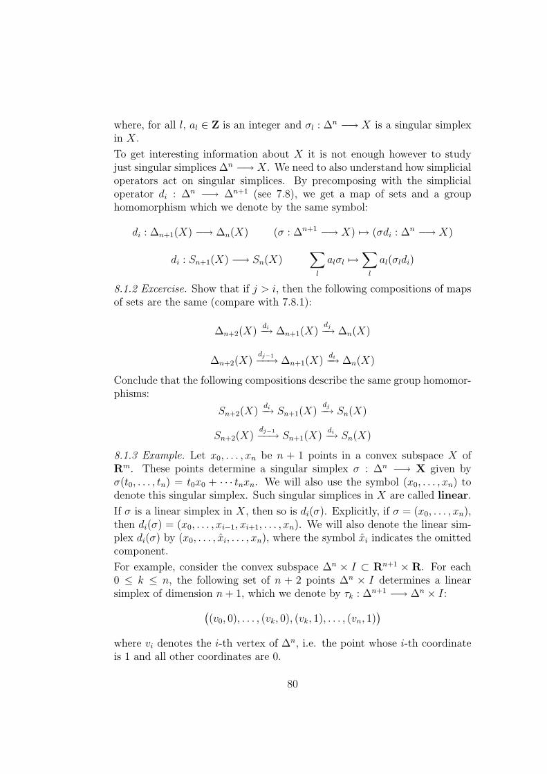
where, for all l, al ∈ Z is an integer and σl : ∆n −→ X is a singular simplexin X.

To get interesting information about X it is not enough however to studyjust singular simplices ∆n −→ X. We need to also understand how simplicialoperators act on singular simplices. By precomposing with the simplicialoperator di : ∆n −→ ∆n+1 (see 7.8), we get a map of sets and a grouphomomorphism which we denote by the same symbol:

di : ∆n+1(X) −→ ∆n(X) (σ : ∆n+1 −→ X) 7→ (σdi : ∆n −→ X)

di : Sn+1(X) −→ Sn(X)∑l

alσl 7→∑l

al(σldi)

8.1.2 Excercise. Show that if j > i, then the following compositions of mapsof sets are the same (compare with 7.8.1):

∆n+2(X)di−→ ∆n+1(X)

dj−→ ∆n(X)

∆n+2(X)dj−1−−→ ∆n+1(X)

di−→ ∆n(X)

Conclude that the following compositions describe the same group homomor-phisms:

Sn+2(X)di−→ Sn+1(X)

dj−→ Sn(X)

Sn+2(X)dj−1−−→ Sn+1(X)

di−→ Sn(X)

8.1.3 Example. Let x0, . . . , xn be n + 1 points in a convex subspace X ofRm. These points determine a singular simplex σ : ∆n −→ X given byσ(t0, . . . , tn) = t0x0 + · · · tnxn. We will also use the symbol (x0, . . . , xn) todenote this singular simplex. Such singular simplices in X are called linear.

If σ is a linear simplex in X, then so is di(σ). Explicitly, if σ = (x0, . . . , xn),then di(σ) = (x0, . . . , xi−1, xi+1, . . . , xn). We will also denote the linear sim-plex di(σ) by (x0, . . . , xi, . . . , xn), where the symbol xi indicates the omittedcomponent.

For example, consider the convex subspace ∆n × I ⊂ Rn+1 × R. For each0 ≤ k ≤ n, the following set of n + 2 points ∆n × I determines a linearsimplex of dimension n+ 1, which we denote by τk : ∆n+1 −→ ∆n × I:(

(v0, 0), . . . , (vk, 0), (vk, 1), . . . , (vn, 1))

where vi denotes the i-th vertex of ∆n, i.e. the point whose i-th coordinateis 1 and all other coordinates are 0.

80

8.1.4 Example. Since ∆0 is the one point space, 0-dimensional singular sim-plices in X can be identified with elements x ∈ X. The group ∆0(X) is thenthe free abelian group generated by elements of X. An element of S0(X) isa combination of elements of X with integer coefficients:

a1x1 + a2x2 + · · ·+ anxn

where ai ∈ Z and xi ∈ X.

Since ∆1 is isomorphic to the interval I, we can think about 1-dimensionalsingular simplices in X also as maps α : I −→ X. Under this identification,if a 1-dimensional simplex σ in X corresponds to α : I −→ X, then d0(σ)corresponds to the end α(1) of the path α. In the same way d1(σ) correspondsto the beginning α(0) of the path α.

8.1.5 Definition. Let n ≥ 0. Define ∂n+1 : Sn+1(X) −→ Sn(X) to be givenby:

∂n+1(σ) =n+1∑i=0

(−1)idi(σ)

8.1.6 Proposition. Let n ≥ 0. The following composition is the zero homo-morphism:

Sn+2(X)∂n+2−−−→ Sn+1(X)

∂n+1−−−→ Sn(X)

Proof.

∂n+1∂n+2(x) =n+1∑j=0

(−1)jdj( n+2∑i=0

(−1)idi(x))

=

=∑j>i

(−1)i+jdjdi(x) +∑j≤i

(−1)i+jdjdi(x) =

use Exercise 8.1.2 to get:

=∑j>i

(−1)i+jdidj−1(x) +∑j≤i

(−1)i+jdjdi(x) =

set j = k + 1 in the first sum to get:

=∑k≥i

(−1)i+k+1didk(x) +∑j≤i

(−1)i+jdjdi(x) = 0

We can now use the above proposition to define a chain complex of abeliangroups:

81

8.1.7 Definition. Let X be a topological space. The following chain complexis called the singular chain complex of X and is denoted by S∗(X):

· · · ∂n+1−−−→ Sn(X)∂n−→ · · · ∂3−→ S2(X)

∂2−→ S1(X)∂1−→ S0(X)

Let G be an abelian group and X a topological space. The n-th homology ofthe complex S∗(X)⊗G is called the n-th homology of X with coefficients inG and is denoted by Hn(X,G).

In the case G is the group of integers Z, then Hn(X,Z) is simply denoted byHn(X) and called the integral homology of X.

8.1.8 Example. Note that S∗(D0) is given by the complex:

· · · id−→ Z0−→ Z

id−→ Z0−→ · · · id−→ Z

0−→ Z

It follows that:

Hn(D0, G) =

{G if n = 0

0 if n > 0

8.1.9 Excercise. Show that there are isomorphisms:

S∗(r∐i=1

D0) =r⊕i=1

S∗(D0) Hn(

r∐i=1

D0, G) =r⊕i=1

Hn(D0, G)

8.1.10 Excercise. As in Example 8.1.4 we think about 1-dimensional singularsimplices in X as paths σ : I −→ X. For such a path, let us denote byσ′ : I −→ X the opposite path, i.e., by definition, σ′(t) := σ(1−t). Show thatσ + σ′ is a boundary in S1(X) (it is in the image of ∂2 : S2(X) −→ S1(X)).

8.1.11 Excercise. Let σ : I −→ X and τ : I −→ X be two paths such thatσ(1) = τ(0). Define σ ∗ τ : I −→ X to be the concatenation of σ and τ ,explicitly:

σ ∗ τ(t) :=

{σ(2t) if 0 ≤ t ≤ 1/2

τ(2− 2t) if 1/2 ≤ t ≤ 1

Show that σ + τ − σ ∗ τ is a boundary in S1(X).

The rest of these notes is devoted to setting up tools to calculate homology ofmore complicated spaces than just discreet spaces. We start with discussing:

82

8.2 Homology and maps

To compare spaces one uses maps. Maps can be also used to compare thehomology groups of spaces. Let f : X −→ Y be a continuous function. Bycomposing with f we get a function between the sets of singular simplices:

∆n(X) 3 (σ : ∆n −→ X) 7→ (fσ : ∆n −→ Y ) ∈ ∆n(Y )

This function is denoted by ∆n(f) : ∆n(X) −→ ∆n(Y ). The induced homo-morphism on the groups of singular simplices is denoted by:

Sn(f) : Sn(X) −→ Sn(Y )

It maps an element a1σ1+· · ·+akσk in Sn(X) to an element a1fσ1+· · ·+akfσkin Sn(Y ).

8.2.1 Excercise. Show that the following diagrams of abelian groups andhomomorphisms commute:

Sn+1(X)Sn+1(f) //

di

��

Sn+1(Y )

di

��Sn(X)

Sn(f) // Sn(Y )

Sn+1(X)Sn+1(f) //

∂n+1

��

Sn+1(Y )

∂n+1

��Sn(X)

Sn(f) // Sn(Y )

8.2.2 Excercise. Let f : X −→ Y and g : Y −→ Z be continuous maps. Showthat the homomorphism Sn(gf) : S∗(X) −→ Sn(Z) is given by the compo-sition of Sn(f) : Sn(X) −→ Sn(Y ) and Sn(g) : Sn(Y ) −→ Sn(Z). Moreovershow that Sn(id) : Sn(X) −→ Sn(X) is the identity homomorphism. Con-clude that if f : X −→ Y is an isomorphism of topological spaces, thenSn(f) : Sn(X) −→ Sn(Y ) is an isomorphism of abelian groups.

From the above exercises it follows that f induces a map of chain complexesS∗(f) : S∗(X) −→ S∗(Y ) and hence a homomorphism of homology groupsHn(f,G) : Hn(X,G) −→ Hn(Y,G). These induced homomorphisms arecompatible with compositions:

S∗(fg) = S∗(f)S∗(g) S∗(id) = id

Hn(fg,G) = Hn(f,G)Hn(g,G) Hn(id, G) = id

Moreover if f : X −→ Y is an isomorphism, then so are S∗(f) and Hn(f,G).

83

8.3 Reduced homology

For any space X, there is a unique map p : X −→ D0. This map inducesthen a homomorphism of chain complexes S∗(p) : S∗(X) −→ S∗(D

0). Weuse this homomorphism to define:

8.3.1 Definition. Let X be a topological space. The kernel of S∗(p) :S∗(X) −→ S∗(D

0) is denoted by S∗(X) and called the complex of reducedsingular simplices of X.

For a group G, the n-th homology of S∗(X)⊗G is denoted by Hn(X,G) andcalled the n-th reduced homology of X with coefficients in G. If G = Z is thegroup of integers, then Hn(X,Z) is simply denoted by Hn(X).

For example, S∗(D0) is the zero complex and consequently Hn(D0, G) = 0

for any n ≥ 0 and any group G.

For any continuous map f : X −→ Y , the following triangle commutes:

Xf //

p

BBB

BBBB

B Yp

~~}}}}

}}}}

D0

By applying S∗ to this triangle, we get a commutative triangle of homomor-phisms of chain complexes:

S∗(X)S∗(f) //

S∗(p)

$$JJJJJJJJJS∗(Y )

S∗(p)

zzttttttttt

S∗(D0)

Commutativity of this diagram implies that Sn(f) : Sn(X) −→ Sn(Y ) takeselements of Sn(X) into elements of Sn(Y ). Thus, for any such continuousmap, restriction of S∗(f) to the subcomplex S∗(X) defines a chain map whichis denoted by:

S∗(f) : S∗(X) −→ S∗(Y )

By tensoring with a group G we get a yet another homomorphism of chaincomplexes:

S∗(f)⊗G : S∗(X)⊗G −→ S∗(Y )⊗GThe induced homomorphism on the n-th homology is denoted by:

Hn(f,G) : Hn(X,G) −→ Hn(Y,G)

84

8.3.2 Excercise. Show that if f : X −→ Y is an isomorphism then so isHn(f,G), for any n ≥ 0 and any group G.

Recall that S∗(D0) can be identified with the complex (see Example 8.1.8):

· · · id−→ Z0−→ Z

id−→ Z0−→ · · · id−→ Z

0−→ Z

Moreover, with this identification, the homomorphism Sn(p) : Sn(X) −→ Zis given by:

Sn(p)(a1σ1 + · · ·+ akσk) = a1 + · · ·+ ak

Thus Sn(X) is the subgroup of Sn(X) consisting of these sums a1σ1 + · · ·+akσk for which a1 + · · ·+ ak = 0.

In the case X is a nonempty space, then there is a map D0 −→ X whosecomposition with p : X −→ D0 is the identity. It follows that after applyingS∗ to these maps we get a commuting diagram:

S∗(D0) //@A BC

id

OOS∗(X)

S∗(p) // S∗(D0)

It then follows that the chain complex S∗(X) is isomorphic to the direct sumof complexes S∗(D0)⊕ S∗(X).

8.3.3 Proposition. Let X be a non empty space and G be a group.

(1) H0(X,G) is isomorphic to G⊕ H0(X,G).

(2) For n > 0, the homomorphism Hn(X,G) −→ Hn(X,G), induced by theinclusion S∗(X) ⊂ S∗(X), is an isomorphism.

Proof. Since X is not empty, the following is a split exact sequence of chaincomplexes:

0 −→ S∗(X) ⊂ S∗(X)S∗(p)−−−→ S∗(D

0) −→ 0

Thus by tensoring with G we get also a split exact sequence of chain com-plexes:

0 −→ S∗(X)⊗G ⊂ S∗(X)⊗G S∗(p)⊗G−−−−−→ S∗(D0)⊗G −→ 0

Such a short exact sequence of chain complexes leads to a long exact sequence

85

of its homologies:

· · · //

// H1(X,G) // H1(X,G)H1(p,G)// H1(D

0, G) //

// H0(X,G) // H0(X,G)H0(p,G)// H0(D

0, G) // 0

The proposition is now a direct consequence of the fact that: H0(D0, G) = G

and Hn(D0, G) = 0 for n > 0.

8.4 H0(X,G)

The aim of this section is to explain what information about a topologicalspace is encoded in its 0’th homology. Note first that, by definition, H0(X)fits into an exact sequence:

S1(X)∂1−→ S0(X) −→ H0(X) −→ 0

Thus an element of H0(X) can be represented by an element in S0(X), i.e.,a sum a1x1 + · · · + akxk where ai ∈ Z and xi ∈ X. Two such sums givethe same element in H0(X) if their difference is of the form ∂1(σ) for someσ ∈ S1(X).

As tensoring is right exact, for any group G, the above exact sequence leadsto an exact sequence:

S1(X)⊗G ∂1−→ S0(X)⊗G −→ H0(X)⊗G −→ 0

It follows that:

8.4.1 Proposition. The groups H0(X,G) and H0(X)⊗G are isomorphic.

A topological space consists of a set X together with a topology (a choiceof open subsets). We used this topology to define an equivalence relation onthe set X: ”being in the same path component” (see Definition 7.13.1).

If 0 and 1 dimensional singular simplices in X are identified with respectivelyelements of X and paths α : I −→ X in X, as explained in Example 8.1.4,then the relation of being in the same path component can be reformulatedas follows:

86

8.4.2 Proposition. Two points x0 ∈ X and x1 ∈ X are in the same pathcomponent if and only if there is a singular simplex σ : ∆1 −→ X such thatd0(σ) = x1 and d1(σ) = x0.

Recall that for x ∈ X, the symbol X[x] denotes the subspace of X consistingof all the points in X that are in the same path component as x.

8.4.3 Proposition. For any G and n ≥ 0, there are isomorphisms:∐[x]∈π0(X)

∆n(X[x]) = ∆n(X)

⊕[x]∈π0(X)

S∗(X[x]) = S∗(X)⊕

[x]∈π0(X)

Hn(X[x], G) = Hn(X,G)

Proof. Since ∆n is path connected, any singular simplex σ : ∆n −→ X maps∆n into one of the path connected components of X. The first isomorphismis then induced by the inclusions X[x] ⊂ X. The second and the thirdisomorphisms are consequences of the first one.

8.4.4 Proposition. If X is non empty and path connected, then, for theunique map p : X −→ D0, the homomorphism H0(p,G) : H0(X,G) −→H0(D

0, G) is an isomorphism.

Proof. Choose a point x ∈ X and consider the composition:

D0 π−→ Xp−→ D0

where π sendsD0 to the chosen point x. Since this composition is the identity,then so is the induced composition on the homology:

H0(D0)

H0(π)−−−→ H0(X)H0(p)−−−→ H0(D

0)

It follows that H0(π) is a monomorphism. We are going to show that it isalso an epimorphism. Let a1x1 + · · · + akxk be an element in S0(X) thatrepresents a given homology class in H0(X). Since X is path connected, forany i, there is a path αi : I −→ X such that αi(0) = x and αi(1) = xi.Consider the following element in S1(X):

σ := a1α1 + · · ·+ akαk

Note that ∂1(σ) = a1x1 + · · · + akxk − (a1 + · · · + ak)x. Consequently theelement a1x1+· · ·+akxk differs from (a1+· · ·+ak)x by en element of the form∂1(σ). This means that the homology class induced by a1x1+· · ·+akxk is the

87

same as the homology class induced by (a1 + · · ·+ak)x. As the latter is in theimage of H0(π), this homomorphism is an epimorphism. We can concludethat H0(π) is an isomorphism. Its inverse H0(p) is therefore an isomorphismtoo. We can now use Proposition 8.4.1 to conclude that H0(p,G) is also anisomorphism for any group G.

8.4.5 Corollary. H0(X,G) =⊕

π0(X)G.

Proof. By Proposition 8.4.3, H0(X,G) =⊕

[x]∈π0(X)H0(X[x]). Since X[x] is

path connected, according to Proposition 8.4.4, H0(X[x]) = G. These twoobservations imply the corollary.

8.5 Homology and homotopy

Not only isomorphisms induce an isomorphism on homology groups. It turnsout that the same is true for homotopy equivalences. This is one of thefundamental properties of the singular chain complexes and their homologygroups.

8.5.1 Theorem. Assume that maps f : X −→ Y and g : X −→ Y arehomotopic. Then the homomorphisms of chain complexes S∗(f) : S∗(X) −→S∗(Y ) and S∗(g) : S∗(X) −→ S∗(Y ) are also homotopic. In particular theinduced homomorphisms Hn(f,G) : Hn(X,G) −→ Hn(Y,G) and Hn(g,G) :Hn(X,G) −→ Hn(Y,G) coincide for all n.

Before we prove this theorem we are going to present some of its conse-quences.

8.5.2 Corollary. (1) If f : X −→ Y is a homotopy equivalence, then forany n ≥ 0 and any group G, Hn(f,G) : Hn(X,G) −→ Hn(Y,G) is anisomorphism.

(2) If X and Y are homotopy equivalent spaces, then, for any n ≥ 0 and anygroup G, the homology groups Hn(X,G) and Hn(Y,G) are isomorphic.

(3) If X is a contractible space, then:

Hn(X,G) =

{G if n = 0

0 if n > 0

88

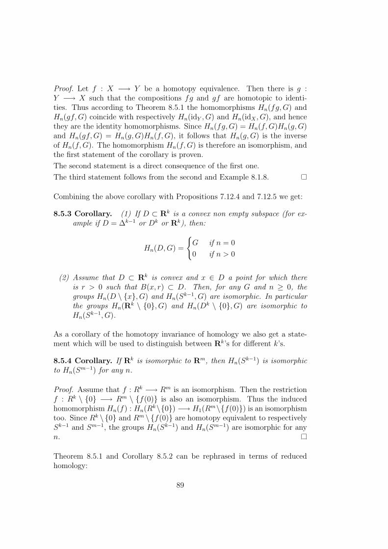
Proof. Let f : X −→ Y be a homotopy equivalence. Then there is g :Y −→ X such that the compositions fg and gf are homotopic to identi-ties. Thus according to Theorem 8.5.1 the homomorphisms Hn(fg,G) andHn(gf,G) coincide with respectively Hn(idY , G) and Hn(idX , G), and hencethey are the identity homomorphisms. Since Hn(fg,G) = Hn(f,G)Hn(g,G)and Hn(gf,G) = Hn(g,G)Hn(f,G), it follows that Hn(g,G) is the inverseof Hn(f,G). The homomorphism Hn(f,G) is therefore an isomorphism, andthe first statement of the corollary is proven.

The second statement is a direct consequence of the first one.

The third statement follows from the second and Example 8.1.8.

Combining the above corollary with Propositions 7.12.4 and 7.12.5 we get:

8.5.3 Corollary. (1) If D ⊂ Rk is a convex non empty subspace (for ex-ample if D = ∆k−1 or Dk or Rk), then:

Hn(D,G) =

{G if n = 0

0 if n > 0

(2) Assume that D ⊂ Rk is convex and x ∈ D a point for which thereis r > 0 such that B(x, r) ⊂ D. Then, for any G and n ≥ 0, thegroups Hn(D \ {x}, G) and Hn(Sk−1, G) are isomorphic. In particularthe groups Hn(Rk \ {0}, G) and Hn(Dk \ {0}, G) are isomorphic toHn(Sk−1, G).

As a corollary of the homotopy invariance of homology we also get a state-ment which will be used to distinguish between Rk’s for different k’s.

8.5.4 Corollary. If Rk is isomorphic to Rm, then Hn(Sk−1) is isomorphicto Hn(Sm−1) for any n.

Proof. Assume that f : Rk −→ Rm is an isomorphism. Then the restrictionf : Rk \ {0} −→ Rm \ {f(0)} is also an isomorphism. Thus the inducedhomomorphism Hn(f) : Hn(Rk\{0}) −→ H1(R

m\{f(0)}) is an isomorphismtoo. Since Rk \{0} and Rm \{f(0)} are homotopy equivalent to respectivelySk−1 and Sm−1, the groups Hn(Sk−1) and Hn(Sm−1) are isomorphic for anyn.

Theorem 8.5.1 and Corollary 8.5.2 can be rephrased in terms of reducedhomology:

89

8.5.5 Corollary. (1) Assume that f : X −→ Y and g : X −→ Y are ho-motopic. Then the homomorphism Hn(f,G) : Hn(X,G) −→ Hn(Y,G)and Hn(g,G) : Hn(X,G) −→ Hn(Y,G) are the same for all n and allgroups G.

(2) If f : X −→ Y is a homotopy equivalence, then Hn(f,G) : Hn(X,G) −→Hn(Y,G) is an isomorphism.

(3) If X and Y are homotopy equivalent, then, for any n ≥ 0 and anygroups G, the reduced homology groups Hn(X,G) and Hn(Y,G) areisomorphic.

(4) If X is contractible, then Hn(X,G) = 0 for any n ≥ 0 and any G.

We now prove Theorem 8.5.1.

Proof of Theorem 8.5.1. We start by defying a sequence of homomorphismssn : Sn(X) −→ Sn+1(Y ). Let S : X×I −→ Y be a homotopy between f andg. Let σ : ∆n −→ X be a singular simplex of dimension n in X. Considerthe composition:

∆n+1 τk−→ ∆n × I σ×id−−−→ X × I S−→ Y

where τk : ∆n+1 −→ ∆n× I is a linear simplex (see Example 8.1.3) given by:

τk =((v0, 0), . . . , (vk, 0), (vk, 1), . . . , (vn, 1)

)(vi denotes the i-th vertex of ∆n). Define:

sn(σ) := Σnk=0(−1)kS(σ × id)(τk)

We claim that the following equality holds:

Sn(g)(σ)− Sn(f)(σ) = ∂n+1sn(σ) + sn−1∂n(σ)

The homomorphisms sn, for n ≥ 0, give therefore a homotopy between S∗(f)and S∗(g).

To show the above equality one uses the same argument for all n’s. Forclarity we will illustrate this calculation only in the case n = 1. The othercases are left as an exercise. Assume that n = 1. Note that:

∂2s1(σ) = ∂2S(σ × id)(τ0)− ∂2S(σ × id)(τ1) =

= S(σ × id)∂2

((v0, 0), (v0, 1), (v1, 1)

)− S(σ × id)∂2

((v0, 0), (v1, 0), (v1, 1)

)=

90

Note that:S(σ × id)∂2

((v0, 0), (v0, 1), (v1, 1)

)=

S(σ×id)((v0, 1), (v1, 1)

)−S(σ×id)

((v0, 0), (v1, 1)

)+S(σ×id)

((v0, 0), (v0, 1)

)and

S(σ × id)∂2

((v0, 0), (v1, 0), (v1, 1)

)=

S(σ×id)((v1, 0), (v1, 1)

)−S(σ×id)

((v0, 0), (v1, 1)

)+S(σ×id)

((v0, 0), (v1, 0)

)It follows that

∂2s1(σ) = S(σ × id)((v0, 1), (v1, 1)

)− S(σ × id)

((v0, 0), (v1, 0)

)+

+S(σ × id)((v0, 0), (v0, 1)

)− S(σ × id)

((v1, 0), (v1, 1)

)On the other hand:

s0∂1(σ) = s0(d0σ)− s0(d1σ) =

= S(d0σ × id)((v0, 0), (v0, 1)

)− S(d1σ × id)

((v0, 0), (v0, 1)

)= S(σ × id)

((v1, 0), (v1, 1)

)− S(σ × id)

((v0, 0), (v0, 1)

)It follows that:

∂2s1(σ) + s0∂1(σ) = S(σ × id)((v0, 1), (v1, 1)

)− S(σ × id)

((v0, 0), (v1, 0)

)As S is a homotopy between f and g, we can then conclude that:

∂2s1(σ) + s0∂1(σ) = S1(g)(σ)− S1(f)(σ)

8.6 Small singular simplices

So far we could only calculate homology in very few cases: the 0-th homologyof an arbitrary space and all homology groups of contractible spaces. Tocalculate the homology of a sphere for example or a circle we need one moretool. This is the subject of this section. The chain complex S∗(X) is simplytoo big for calculations. Our strategy is to find a much smaller subcomplexof S∗(X) that has the same homology as S∗(X).

Let X be a topological space. Let us fix an open cover of X, i.e., a familyU = {Ui} of open subsets of X such that X =

⋃Ui.

91

8.6.1 Definition. An U-singular simplex in X of dimension n is a contin-uous map σ : ∆n −→ X such that for some i, the image σ(∆n) is includedin Ui.

The set of U-singular simplexes of dimension n in X is denoted by ∆Un (X).

The symbol SUn (X) denotes the free abelian groups generated by the set ∆Un (X).

Note that if σ : ∆n −→ X is an U -singular simplex in X, then so is diσ. Itfollows that the homomorphism ∂n+1 : Sn+1(X) −→ Sn(X) takes elementsof SUn+1(X) into SUn (X). In this way we obtain a chain subcomplex of S∗(X)denoted by SU∗ (X). Explicitly it is given by:

· · · ∂n+2−−−→ SUn+1(X)∂n+1−−−→ · · · ∂2−→ SU1 (X)

∂1−→ SU0 (X)

It turns out that to calculate homology of a space we can use both thecomplex of singular simplices or the complex of U -singular simplexes. Thisis the content of:

8.6.2 Theorem. Let U be an open cover of a topological space X. Then theinclusion i : SU∗ (X) ⊂ S∗(X) is a homotopy equivalence, i.e., there is a chaincomplex homomorphism s : S∗(X) −→ SU∗ (X) such that the compositionsis : S∗(X) −→ S∗(X) and si : SU∗ (X) −→ SU∗ (X) are homotopic to identities.

This theorem together with the homotopy invariance of homology (Theo-rem 8.5.1) will be our key tools to calculate homology of spaces. The rest ofthese notes explain how to use this theorem in practise. We start with:

8.6.3 Corollary. For any group G and any n ≥ 0, the groups Hn(X,G) andHn(SU∗ (X)⊗G) are isomorphic.

8.6.4 Excercise. Consider the following subsets of S1:

U0 := {(x, y) ∈ S1 | y > −1/2} U1 := {(x, y) ∈ S1 | y < 1/2}

They form an open cover U = {U0, U1} of S1. Consider also a singularsimplex σ : I −→ S1 given by the formula σ(t) = (sin(2tπ), cos(2tπ)). Is σ aU -singular simplex? Find a singular simplex τ ∈ SU1 (S1) such that τ − σ isa boundary in S1(S

1), i.e., it is in the image of ∂2 : S2(S1) −→ S1(S

1).

8.7 Reduced small singular simplices

Let U be an open cover of X. Define SU∗ (X) to be the kernel of the compo-sition:

SU∗ (X) ⊂ S∗(X)S∗(p)−−−→ S∗(D

0)

92

The group SUn (X) is then the subgroup of S∗(X) consisting of these combina-tions of U -singular simplices a1σ1+· · ·+akσk for which the sum a1+· · ·+ak =0. It is a subgroup of the reduced complex Sn(X).

8.7.1 Excercise. Assume that X is not an empty space. Show that the chaincomplexes S∗(X), S∗(X), SU∗ (X), SU∗ (X), and S∗(D

0) fit into the followingcommutative diagram of chain complexes whose rows are split exact:

0 // SU∗ (X)� � //

� _

��

SU∗ (X) //� _

��

S∗(D0) //

id��

0

0 // S∗(X)� � // S∗(X)

S∗(p) // S∗(D0) // 0

8.7.2 Excercise. Show that the inclusion SU∗ (X) ⊂ S∗(X) is a homotopyequivalence of chain complexes (use Theorem 8.6.2).

Using the above exercises and Theorem 8.6.2, we can rephrase Proposi-tion 8.3.3 in terms of the U -singular simplices:

8.7.3 Proposition. Let X be a non empty space, U its open cover, and Ga group.

(1) H0(X,G) is isomorphic to G⊕H0(SU∗ (X)⊗G).

(2) For n > 0, the homomorphism Hn(SU∗ (X)⊗G) −→ Hn(X,G), inducedby the inclusion SU∗ (X) ⊂ S∗(X), is an isomorphism.

The key point of the above proposition is that to calculate homology of X,instead of using the complex S∗(X), me can use SU∗ (X) for some open cover Uof X. Why is it easier to use the complexes SU∗ (X) or SU∗ (X)? The answer isthat they often lead to exact sequences. Let us illustrate this in the basic caseof an open cover U = {U0, U1} of X that consists of only two open subsets.This will be the case used in the rest of these notes. Let V = U0 ∩ U1 andassume that V is not empty. We are going to use the following symbols todenote the appropriate inclusions:

V� � j0 //

� _

j1��

U0� _

i1��

U1� � i0 // X

Observe that the inclusions i0 : U0 ⊂ X and i1 : U1 ⊂ X map singularsimplices in Ui into U -singular simplexes of X. Moreover any U -singular

93

simplexes of X is in the image of S∗(i0) or S∗(i1). This means that thefollowing homomorphism is an epimorphism:

S∗(i0)⊕ S∗(i1) : S∗(U0)⊕ S∗(U1) −→ SU∗ (X)

What is the kernel of this homomorphism? A pair (x, y) ∈ S∗(U0) ⊕ S∗(U1)is in the kernel of S∗(i0)⊕ S∗(i1) if and only if S∗(i0)(x) = −S∗(i1)(y). Thiscan happen if and only if x is in the image of both S∗(j0) : S∗(V ) −→ S∗(U0)and S∗(j1) : S∗(V ) −→ S∗(U1). This leads to an exact sequence of chaincomplexes:

0 −→ S∗(V )(S∗(j0),−S∗(j1))−−−−−−−−−→ S∗(U0)⊕ S∗(U1)

S∗(i0)+S∗(i1)−−−−−−−−→ SU∗ (X) −→ 0

8.7.4 Excercise. Show that the above sequence is a part of the followinglarger commutative diagram of chain complexes whose all rows and columnsare exact:

0

��

0

��

0

��

0 // S∗(V )(S∗(j0),−S∗(j1))//

� _

��

S∗(U0)⊕ S∗(U1)S∗(i0)+S∗(i1) //

� _

��

SU∗ (X) //� _

��

0

0 // S∗(V )(S∗(j0),−S∗(j1))//

S∗(p)��

S∗(U0)⊕ S∗(U1)S∗(i0)+S∗(i1) //

S∗(p)⊕S∗(p)��

SU∗ (X) //

S∗(p)��

0

0 // S∗(D0)

(id,−id) //

��

S∗(D0)⊕ S∗(D0)

id+id //

��

S∗(D0) //

��

0

0 0 0

Since all the groups in the above diagram are free, we can tensor this diagramwith a group G and get analogous diagram whose rows and columns are alsoexact. We will be interested only in its top row. For any group G we thenhave an exact sequence of chain complexes:

0 // S∗(V )⊗G // (S∗(U0)⊗G)⊕(S∗(U1)⊗G) // SU∗ (X)⊗G // 0

Such an exact sequence of chain complexes leads to a long exact sequence of

94

their homologies:

· · · // H2(X,G)

qqccccccccccccccccccccccccccccccccccccccccccccccccccccccccccc

H1(V,G)(H1(j0,G),−H0(j1,G))

// H1(U0, G)⊕ H1(U1, G)H1(i0,G)+H1(i1,G) // H1(X,G)

qqccccccccccccccccccccccccccccccccccccccccccccccccccccccccccc

H0(V,G)(H0(j0,G),−H0(j1,G))

// H0(U0, G)⊕ H0(U1, G)H0(i0,G)+H0(i1,G) // H0(X,G)

qqccccccccccccccccccccccccccccccccccccccccccccccccccccccccccccccc

0

We can now use this exact sequence to relate homologies of X, U0, U1, andV . For example, assume that U0 and U1 are contractible spaces. In this caseHn(U0, G) = Hn(U1, G) = 0 for any n and thus the above exact sequencegives:

8.7.5 Proposition. Let U = {U0, U1} be an open cover of X and G be agroup. Assume that V = U0 ∩ U1 is not empty and that U0 and U1 arecontractible. Then, H0(X,G) = 0 and, for n > 0, Hn(X,G) = Hn−1(V,G).

If only one of {U0, U1} is contractible, for example U1, then again sinceHn(U1, G) = 0, for all n, the above exact sequence gives:

8.7.6 Proposition. Let U = {U0, U1} be an open cover of X and G be agroup. Assume that V = U0 ∩ U1 is not empty and that U1 is contractible.Then there is an exact sequence:

· · · // H2(X,G)

rrdddddddddddddddddddddddddddddddddddddddddddddd

H1(V,G)H1(j0,G

// H1(U0, G)H1(i0,G) // H1(X,G)

rrdddddddddddddddddddddddddddddddddddddddddddddd

H0(V,G)H0(j0,G)

// H0(U0, G)H0(i0,G) // H0(X,G)

qqdddddddddddddddddddddddddddddddddddddddddddddddddd

0

95

8.8 Homology of spheres

We already know that, since S0 is a discreet space consisting of two points,then:

Hn(S0, G) =

{G⊕G if n = 0

0 if n > 0

Hn(S0, G) =

{G if n = 0

0 if n > 0

The aim of this section is to prove:

8.8.1 Theorem. Let G be a group. Then:

Hn(Sk, G) =

{G if n = k

0 if n 6= k

Proof. The proof is by induction on k. The case k = 0 has already beenproven. Let k > 0. We are going to use the following open subsets of Sk:

U0 = {(x1, . . . xk+1) ∈ Sk | xk+1 > −1/2}

U1 = {(x1, . . . xk+1) ∈ Sk | xk+1 < 1/2}

V = U0 ∩ U1 = {(x1, . . . xk+1) ∈ Sk | − 1/2 < xk+1 < 1/2}

First we need to understand the homotopy type of these subspaces:

8.8.2 Excercise. (1) Show that U0 and U1 are contractible spaces.

(2) Show that U0 and U1 are isomorphic to Rk.

(3) Show that the following inclusion is a homotopy equivalence:

Sk−1 3 (x1, . . . , xk) 7→ (x1, . . . , xk, 0) ∈ V

From the above exercise it follows that the cover U = {U0, U1} consists ofcontractible spaces. We can then use Proposition 8.7.5 to conclude thatH0(S

k, G) = 0 and, for n > 0, Hn(Sk, G) = Hn−1(V,G). However since V ishomotopic to Sk−1, we get that for n > 0:

Hn(Sk, G) = Hn−1(Sk−1, G)

We can now use the inductive assumption to finish the proof of the theorem.

96

8.8.3 Corollary. Let k > 0 and G be a group. Then:

Hn(Sk, G) =

{G if n = 0 or n = k

0 if n 6= 0 and n 6= k

8.8.4 Excercise. Let σ : I −→ S1 be a map given by the formula σ(t) =(sin(2tπ), cos(2tπ)

). It is a singular simplex in S1(S

1). Show that it is acycle, i.e., it is in the kernel of ∂1 : S1(S

1) −→ S0(S1). Show moreover, that

its homology class [σ] ∈ H1(S1) = Z is a generator.

8.8.5 Excercise. Let τ : I −→ S1 be a map given by the formula σ(t) =(sin(4tπ), cos(4tπ)

). It is a singular simplex in S1(S

1). Show that it is acycle, i.e., it is in the kernel of ∂1 : S1(S

1) −→ S0(S1). Show moreover

that τ − 2σ, were σ is defined as in Exercise 8.8.4, is a boundary, i.e., it isin the image of ∂2 : S2(S

1) −→ S1(S1). Conclude that the homology class

[τ ] ∈ H1(S1) is equal to 2[σ] ∈ H1(S

1).

8.8.6 Excercise. Let us think about S1 as a subspace of complex numbers C,of length 1. Let α : S1 −→ S1 be the squaring map α(z) := z2. Show thatH1(α) : H1(S

1) −→ H1(S1) is multiplication by 2. Show that the same holds

for the homomorphism H1(α,G) : H1(S1, G) −→ H1(S

1, G), for any groupG.

8.8.7 Excercise. Let σ be as defined in Exercise 8.8.4. Let σ′ : I −→ S1

be given by σ′(t) =(

sin(2π(1 − t), cos(2π(1 − t)). Show that σ′ is a cycle.

Show further that σ + σ′ is a boundary in S1(S1), i.e., it is in the image of

∂2 : S2(S1) −→ S1(S

1). Conclude that the homology class [σ′] ∈ H1(S1) is a

generator and [σ′] = −[σ].

8.8.8 Excercise. Let β : S1 −→ S1 be the map given by the formula β(x1, x2) =(x1,−x2). Show that H1(β) : H1(S

1) −→ H1(S1) is the multiplication by

−1.

8.9 Some geometric applications

In this section we present some geometric applications and corollaries of thecalculation presented in Theorem 8.8.1. We start with:

8.9.1 Proposition. Sk is homotopy equivalent to Sm if and only if k = m.

Proof. If k = m, then Sk is even isomorphic to Sm. Assume that Sk ishomotopy equivalent to Sm. Then the homology groups Hn(Sk) and Hn(Sm)are then isomorphic for all n. According to Theorem 8.8.1, this can happenif and only if k = m.

97

We have now enough tools to show:

8.9.2 Proposition. Rk is isomorphic to Rm if and only if k = m.

Proof. If k = m, then obviously Rk is isomorphic to Rm. Assume that Rk

and Rm are isomorphic. By Corollary 8.5.4 we then have that Hn(Sk−1) andHn(Sm−1) are isomorphic groups for all n. Using Proposition 8.9.1 we canthen conclude that k − 1 = m− 1, and hence k = m.

8.9.3 Excercise. Let M be a manifold of dimension m and N be a manifold ofdimension k (see Definition 7.11.1). Show that if M and N are isomorphic,then m = k.

8.9.4 Proposition. Let k ≥ 1. There is no map r : Dk −→ Sk−1 forwhich the composition of the inclusion Sk−1 ⊂ Dk and r is homotopic toid : Sk−1 −→ Sk−1.

Proof. Assume that such a map exists. Consider its effect on homology:

Hk−1(Sk−1) −→ Hk−1(D

k)Hk−1(r)−−−−→ Hk−1(S

k−1)

Note that this composition must be the identity. Thus we would get a com-mutative diagram of the form:

Z //@A BCid

OO0 // Z

This however is impossible (why?).

8.9.5 Proposition. Let f : Dk −→ Dk be a continuous map. Then there isa point x ∈ Dk, such that f(x) = x.

Proof. The case k = 0 is obvious. Assume that k ≥ 1 and that there isno such point, i.e., for all x ∈ Dk, f(x) 6= x. We can then define a mapr : Dk −→ Sk−1 by the formula:

r(x) :=x− f(x)

|x− f(x)|

We are going to show that the composition of the inclusion Sk−1 ⊂ Dk andr is homotopic to the identity. We can then use Proposition 8.9.4 to get acontradiction. Define the homotopy H : Sk−1 × I −→ Sk−1 by the formula:

H(x, t) :=x− tf(x)

|x− tf(x)|This is well defined since x− tf(x) 6= 0 (why?). Note that H(x, 0) = x andH(x, 1) is the discussed composition.

98

8.9.6 Excercise. Let f : S2k −→ S2k be a continuous map. Show that thereis a point x ∈ S2k such that either f(x) = x or f(x) = −x. Is the same truefor an odd dimensional sphere?

8.10 The homology of the antipodal map

The aim of this section is to determined the effect on the k-th homologygroup of the antipodal map an : Sk −→ Sk. By definition an : Sk −→ Sk isthe map given by the formula:

an(x1, . . . , xk+1) := (−x1, . . . ,−xk+1)

Let k ≥ 1 and k + 1 ≥ i ≥ 1. Define the map fi : Sk −→ Sk to be given bythe formula:

fi(x1, . . . , xi−1, xi, xi+1, . . . , xk+1) = (x1, . . . , xi−1,−xi, xi+1, . . . , xk+1)

We first determine the effect of fi on the k-homology group:

8.10.1 Proposition. Let k ≥ 1 and k + 1 ≥ i ≥ 1. For any group G, thehomomorphism Hk(fi, G) : Hk(S

k, G) −→ Hk(Sk, G) is the multiplication by

−1.

Proof. The proof is by induction on k. The case k = 1 has been the subjectof Exercise 8.8.8. Assume that k > 1. Let us choose j 6= i. As in the proofof Theorem 8.8.1, let:

U0 = {(x1, . . . xk+1) ∈ Sk | xj > −1/2}

U1 = {(x1, . . . xk+1) ∈ Sk | xj < 1/2}V = U0 ∩ U1 = {(x1, . . . xk+1) ∈ Sk | − 1/2 < xj < 1/2}

Note that fi : Sk −→ Sk maps U0 to U0 and U1 to U1. Moreover re-stricted to Sk−1 = {(x1, . . . , xj−1, 0, xj+1, . . . , xk+1) ∈ V ⊂ Sk} the map fi isthe analogous map to fi, but for Sk−1. Thus by the inductive assumptionHk−1(fi, G) : Hk−1(V,G) −→ Hk−1(V,G) is multiplication by −1. Considernext the following commutative diagram of chain complexes, whose rows areexact:

0 // S∗(V )(S∗(j0),−S∗(j1))//

S∗(fi)

��

S∗(U0)⊕ S∗(U1)S∗(i0)⊕S∗(i1)//

S∗(fi)⊕S∗(fi)

��

SU∗ (Sk) //

S∗(fi)

��

0

0 // S∗(V )(S∗(j0),−S∗(j1))// S∗(U0)⊕ S∗(U1)

S∗(i0)⊕S∗(i1)// SU∗ (Sk) // 0

99

This leads to a commutative square, as in Proposition 8.7.5, with exact rows:

0 // Hk(Sk, G)

Hk(fi,G)��

∂ // Hk−1(V,G) //

Hk−1(fi,G)

��

0

0 // Hk(Sk, G)

∂ // Hk−1(V,G) // 0

where ∂ : Hk(Sk, G) −→ Hk−1(V,G) is the connecting homomorphism in-

duces by the short exact sequence of chain complexes above. Since by theinductive assumption Hk−1(fi, G) : Hk−1(V,G) −→ Hk−1(V,G) is multipli-cation by −1 and ∂ is an isomorphism, then Hk(fi, G) : Hk(S

k, G) −→Hk(S

k, G) is also the multiplication by −1 homomorphism.

8.10.2 Corollary. Let k ≥ 1. The homomorphism Hk(an, G) : Hk(Sk, G) −→

Hk(Sk, G) is multiplication by (−1)k+1.

Proof. Note that an is the composition of fi for k + 1 ≥ i ≥ 1, i.e.,:

an = fk+1fk · · · f1

Thus:

Hk(an, G) = Hk(fk+1, G)Hk(fk, G) · · ·Hk(f1, G)

Since, by Proposition 8.10.1, Hk(fi, G) : Hk(Sk, G) −→ Hk(S

k, G) is themultiplication by −1, for all i, the corollary follows.

8.11 The effect on homology of a cell attach-

ment

Assume that we know the homology of X and the effect on homology groupsof the map α : Sk−1 −→ X. Is this information enough to determine thehomology of the space X ∪α Dk (see Section 7.9)? Let i : X ⊂ X ∪α Dk bethe inclusion map.

8.11.1 Theorem. Let k ≥ 1, α : Sk−1 −→ X be a map, and G be a group.

(1) If n 6= k− 1 and n 6= k, then Hn(i, G) : Hn(X,G) −→ Hn(X ∪αDk, G)is an isomorphism.

100

(2) There is an exact sequence of abelian groups:

0 // Hk(X,G)Hk(i,G) // Hk(X ∪α Dk, G)

rrddddddddddddddddddddddddddddddddddddd

Hk−1(Sk−1, G)

Hk−1(α,G)

// Hk−1(X,G)Hk−1(i,G)// Hk−1(X ∪α Dk, G)

qqdddddddddddddddddddddddddddddddddddddddddd

0

Proof. Define the following open subsets of X ∪α Dk:

U0 := X∐{x ∈ Bk | |x| > 1/3}

U1 := {x ∈ Bk | 2/3 > |x|}V := U0 ∩ U1 = {x ∈ Bk | 2/3 > |x| > 1/3}

We need to understand the homotopy type of these subspaces:

8.11.2 Excercise. Show that the inclusion X ⊂ U0 is a homotopy equivalence.

8.11.3 Excercise. Show that U1 is a contractible space and that the inclusion:

{x ∈ V | |x| = 1/2} ⊂ V

is a homotopy equivalence. Conclude that V is homotopy equivalent to Sk−1.

8.11.4 Excercise. Let S := {x ∈ V | |x| = 1/2} and f : Sk−1 −→ S bedefined by the formula f(x) = x/2. Show that the following compositionsare homotopic:

Sk−1 f−→ S ⊂ V ⊂ U0

Sk−1 α−→ X ⊂ U0

It is clear that U := {U0, U1} is an open cover of X ∪α Dk. Since U1 iscontractible and V is not empty we can use Proposition 8.7.6 to get an exactseduce:

· · · // H2(X ∪α Dk, G)

qqdddddddddddddddddddddddddddddddddddddddddddddd

H1(V,G)H1(j0,G)

// H1(U0, G)H1(i0,G) // H1(X ∪α Dk, G)

qqdddddddddddddddddddddddddddddddddddddddddddddd

H0(V,G)H0(j0,G)

// H0(U0, G)H0(i0,G) // H0(X ∪α Dk, G)

qqcccccccccccccccccccccccccccccccccccccccccccccccccc

0

101

Since V is homotopy equivalent to Sk−1, if n 6= k and n 6= k−1, the homologygroups Hn(V,G) and Hn−1(V,G) are trivial. It follows that the homomor-phism Hn(i0, G) : Hn(U0, G) −→ Hn(X ∪αDk, G) is an isomorphism. As theinclusion X ⊂ U0 is a homotopy equivalence, we can conclude that, for n 6= kand n 6= k−1, the homomorphism Hn(i, G) : Hn(X,G) −→ Hn(X ∪αDk, G)is an isomorphism. It then follows that so is Hn(i, G) : Hn(X,G) −→Hn(X ∪α Dk, G).

In the case n = k or n = k − 1, the above exact sequence becomes:

0 // Hk(U0, G)Hk(i0,G) // Hk(X ∪α Dk, G)

rrddddddddddddddddddddddddddddddddddddd

Hk−1(V,G)Hk−1(j0,G)

// Hk−1(U0, G)Hk−1(i0,G)// Hk−1(X ∪α Dk, G)

rrddddddddddddddddddddddddddddddddddddddddd

0

Using Exercise 8.11.4, we get the claimed exact sequence.

8.12 The integral homology groups of the pro-

jective spaces

In this section we will determine the integral homology of the projectivespaces RPn. Since RP1 = S1, we then have:

Hn(RP1,Z) =

{Z if n = 1

0 if n 6= 1

The aim of this section is to prove:

8.12.1 Theorem. Let k ≥ 0. Then:

(1) if k is even

Hn(RPk,Z) =

{Z/2 if n is odd and n < k

0 if n is even or n ≥ k

(2) if k is odd

Hn(RPk,Z) =

Z/2 if n is odd and n < k

0 if n is even or n > k

Z if n = k

102

First, we are going to prove several supporting statements. Let k ≥ 1. Recallthat π : Sk−1 −→ RPk−1 is the map that sends the vector v to the line in Rk

spanned by v. This map is used to build the next projective space. Accordingto Proposition 7.10.3 there is an isomorphism:

RPk = RPk−1 ∪π Dk

Let i : RPk−1 ⊂ RPk be the standard inclusion. According to Theo-rem 8.11.1.(1) we get:

8.12.2 Lemma. Let k ≥ 1. If n 6= k − 1 and n 6= k, then Hn(i) :Hn(RPk−1) −→ Hn(RPk) is an isomorphism. In particular, for n ≥ 2:

0 = Hn(S1) = Hn(RP1) = · · · = Hn(RPn−1)

Theorem 8.11.1.(2) gives also an exact sequence:

0 // Hk(RPk−1)Hk(i) // Hk(RPk)

∂eeeeeeeeeeeeeeeeeeee

rreeeeeeeeeeeeeeeeeee

Hk−1(Sk−1)

Hk−1(π)

// Hk−1(RPk−1)Hk−1(i) // Hk−1(RPk)

rrddddddddddddddddddddddddddddddddddddddddddd

0

With a help of Lemma 8.12.2 this sequence becomes:

0 // 0 // Hk(RPk)

∂eeeeeeeeeeeeeeeeeeee

rreeeeeeeeeeeeeeeeeee

Hk−1(Sk−1)

Hk−1(π)

// Hk−1(RPk−1)Hk−1(i) // Hk−1(RPk)

rrddddddddddddddddddddddddddddddddddddddddddd

0

It follows that Hk(RPk) is a subgroup of Hk(Sk−1) = Z, and consequently

it is either 0 or is isomorphic to Z. We are going to show that this dependson the parity of k.

To calculate the homology of projective spaces we thus need to understandthe homomorphisms Hk(π) : Hk(S

k) −→ Hk(RPk) and ∂ : Hk(RPk) −→Hk−1(S

k−1) for various k’s. To do that we will analyze the following open

103

covers of RPk and Sk. Let k ≥ 1. Let U = {U0, U1} be an open cover ofRPk given, as in the previous section, by:

U0 := RPk−1∐{x ∈ Bk | |x| > 1/3}

U1 := {x ∈ Bk | 2/3 > |x|}

Define:

V := U0 ∩ U1 = {x ∈ Bk | 2/3 > |x| > 1/3}S := {x ∈ V | |x| = 1/

√3} ⊂ V

W0 := π−1(U0) ⊂ Sk

W1 := π−1(U1) ⊂ Sk

Z0 := {(x1, . . . , xk+1) ∈ Sk | xk+1 >√

5/3} ⊂ Sk

Z1 := {(x1, . . . , xk+1) ∈ Sk | xk+1 < −√

5/3} ⊂ Sk

Y := W0 ∩W1 ⊂ Sk

Y0 := {(x1, . . . , xk+1) ∈ Sk |√

8/3 > xk+1 >√

5/3} ⊂ Sk

Y1 := {(x1, . . . , xk+1) ∈ Sk | −√

8/3 < xk+1 < −√

5/3} ⊂ Sk

S0 := {(x1, . . . , xk+1) ∈ Sk | xk+1 =√

6/3} ⊂ Sk

S1 := {(x1, . . . , xk+1) ∈ Sk | xk+1 = −√

6/3} ⊂ Sk

8.12.3 Excercise. Show that:

(1) W0 = {(x1, . . . , xk+1) ∈ Sk | |xk+1| <√

8/3}

(2) W1 = Z0 ∪ Z1

(3) Y = Y0 ∪ Y1

8.12.4 Excercise. (1) Show that S ⊂ V and all the following inclusions arehomotopy equivalences:

S0� � // Y0

� � //W0 Y1? _oo S1

? _oo

(2) Z0 and Z1 are contractible spaces.

8.12.5 Excercise. (1) Show that π takes S0 and S1 into S and that theinduced maps π : S0 −→ S and π : S1 −→ S are isomorphisms.

(2) Show that the following formulas define continuous maps:

s0 : Sk−1 −→ S0 s1 : Sk−1 −→ S1 s : Sk−1 −→ S

s0(x) := (x/√

3,√

6/3) s1(x) := (x/√

3,−√

6/3) s(x) = x/√

3

104

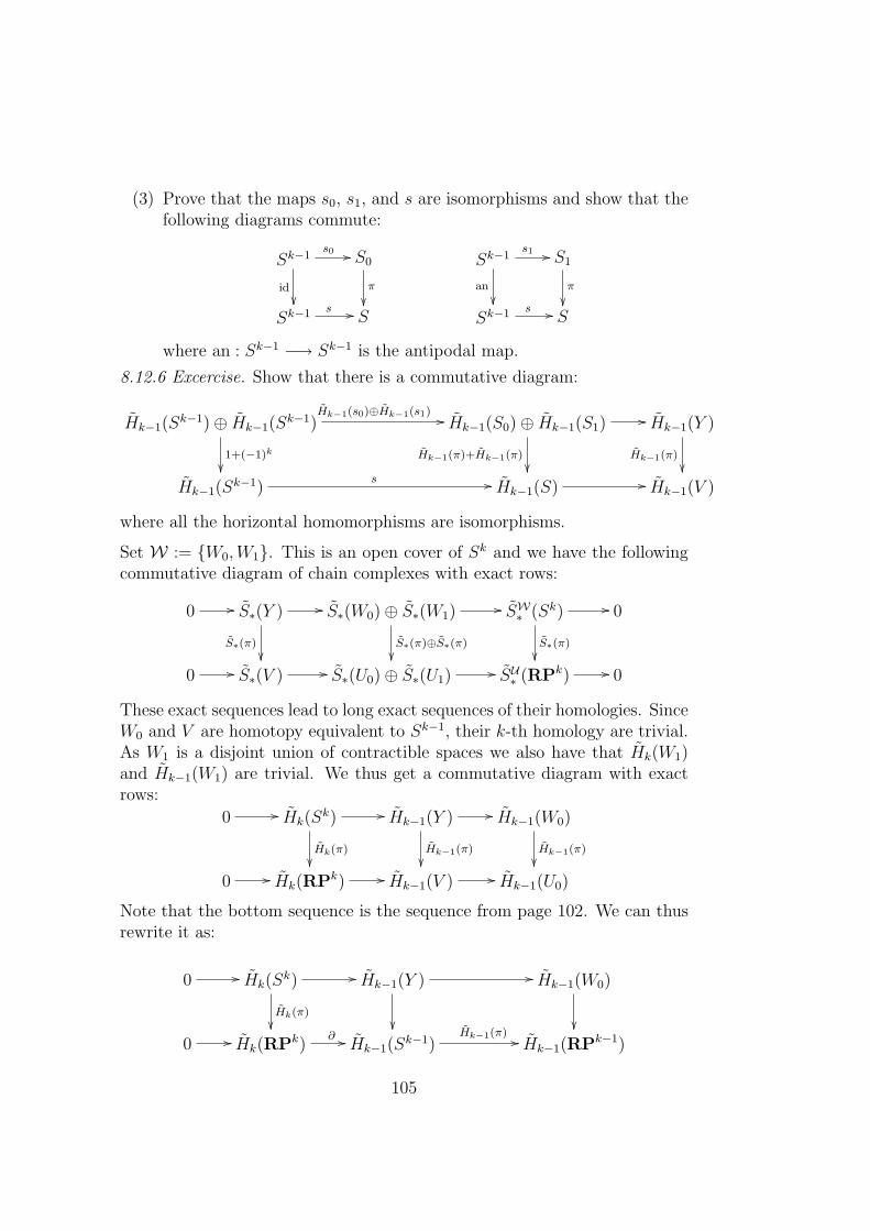
(3) Prove that the maps s0, s1, and s are isomorphisms and show that thefollowing diagrams commute:

Sk−1s0 //

id��

S0

π

��Sk−1 s // S

Sk−1s1 //

an

��

S1

π

��Sk−1 s // S

where an : Sk−1 −→ Sk−1 is the antipodal map.

8.12.6 Excercise. Show that there is a commutative diagram:

Hk−1(Sk−1)⊕ Hk−1(S

k−1)Hk−1(s0)⊕Hk−1(s1) //

1+(−1)k

��

Hk−1(S0)⊕ Hk−1(S1) //

Hk−1(π)+Hk−1(π)��

Hk−1(Y )

Hk−1(π)��

Hk−1(Sk−1)

s // Hk−1(S) // Hk−1(V )

where all the horizontal homomorphisms are isomorphisms.

Set W := {W0,W1}. This is an open cover of Sk and we have the followingcommutative diagram of chain complexes with exact rows:

0 // S∗(Y )

S∗(π)��

// S∗(W0)⊕ S∗(W1) //

S∗(π)⊕S∗(π)��

SW∗ (Sk)

S∗(π)��

// 0

0 // S∗(V ) // S∗(U0)⊕ S∗(U1) // SU∗ (RPk) // 0

These exact sequences lead to long exact sequences of their homologies. SinceW0 and V are homotopy equivalent to Sk−1, their k-th homology are trivial.As W1 is a disjoint union of contractible spaces we also have that Hk(W1)and Hk−1(W1) are trivial. We thus get a commutative diagram with exactrows:

0 // Hk(Sk) //

Hk(π)��

Hk−1(Y ) //

Hk−1(π)��

Hk−1(W0)

Hk−1(π)��

0 // Hk(RPk) // Hk−1(V ) // Hk−1(U0)

Note that the bottom sequence is the sequence from page 102. We can thusrewrite it as:

0 // Hk(Sk) //

Hk(π)��

Hk−1(Y ) //

��

Hk−1(W0)

��

0 // Hk(RPk)∂ // Hk−1(S

k−1)Hk−1(π) // Hk−1(RPk−1)

105

If we identify the appropriate groups with Z and use Exercise 8.12.6, theabove commutative diagram becomes:

0 // Hk(Sk) //

Hk(π)��

Z⊕ Z

1+(−1)k

��

1+1 // Z

��

0 // Hk(RPk) // Z // Hk−1(RPk−1)

In this diagram, the generator of Hk(Sk) is mapped to an element (1,−1) ∈

Z⊕Z via the horizontal homomorphism. It follows that we get a commutativediagram:

Z = Hk(Sk)Hk(π) //@A BC

1+(−1)k+1

OOHk(RPk)

∂ // Hk−1(Sk−1) = Z

We can thus conclude:

8.12.7 Corollary. If k is odd, then the image of the following compositionis given by the subgroup generated by 2:

Z = Hk(Sk)

Hk(π)−−−→ Hk(RPk)∂−→ Hk(S

k−1) = Z

In particular the homomorphism Hk(π) : Hk(Sk) −→ Hk(RPk) is a monomor-

phism.

Recall that we have an exact sequence:

0 // 0 // Hk(RPk)

∂eeeeeeeeeeeeeeeeeee

rreeeeeeeeeeeeeeeeeee

Hk(Sk−1)

Hk−1(π)

// Hk−1(RPk−1)Hk−1(i) // Hk−1(RPk)

rrdddddddddddddddddddddddddddddddddddddddddd

0

Using this exact sequence and Corollary 8.12.7 we get:

8.12.8 Corollary. Let k ≥ 1.

(1) If k is even, then Hk(RPk) = 0.

(2) If k is odd, then ∂ : Hk(RPk) −→ Hk−1(Sk−1) is an isomorphism. In

particular Hk(RPk) is isomorphic to Z.

106

Proof. The proof is by induction on k. Case k = 1 is left as an exercise (usethe above exact sequence and observe that H0(RP0) = H0(RP1) = 0).

Assume that k > 1 and that the lemma is true for projective spaces whosedimension is less than k. If k is even, then k − 1 is odd and and hence byCorollary 8.12.7, Hk−1(π) : Hk(S

k−1) −→ Hk−1(RPk−1) is a monomorphism.Its kernel Hk(RPk) is therefore trivial.

Assume that k is odd. Thus k − 1 is even and by the inductive assumptionHk−1(RPk−1) = 0. It then follows that the boundary homomorphism: ∂ :Hk(RPk) −→ Hk−1(S

k−1) is an isomorphism.

We can now identify explicitly the image of:

8.12.9 Lemma. Let k ≥ 1 be odd. Then the image of:

Z = Hk(Sk)

Hk(π)−−−→ Hk(RPk) = Z

is the subgroup generated by 2.

Proof. Recall that since k is odd, we have a commutative diagram:

Z = Hk(Sk)

Hk(π) //@A BC2

OOHk(RPk)

∂ // Hk−1(Sk−1) = Z

The lemma now is a consequence of the fact that the boundary homomor-phism ∂ : Hk(RPk) −→ Hk−1(S

k−1) is an isomorphism.

We are now ready to prove:

Proof of Theorem 8.12.1. By Lemma 8.12.2 and Corollary 8.12.8 we alreadyknow that the theorem is true when n ≥ k ≥ 1. It remains to prove thetheorem for n < k. This will be done by induction on k. The case k = 1 isclear. Let k > 1 and assume that the theorem is true for projective spaceswhose dimension is smaller than k. Since Hn(i) : Hn(RPk−1) −→ Hn(RPk)is an isomorphism for n 6= k and n 6= k − 1, by the inductive assumption wethen know that the theorem is true for n ≤ k − 2. It remains to show thatthe theorem is also true for n = k−1. Recall that there is an exact sequence:

0 // 0 // Hk(RPk)

∂eeeeeeeeeeeeeeeeeeee

rreeeeeeeeeeeeeeeeeee

Hk−1(Sk−1)

Hk−1(π)

// Hk−1(RPk−1)Hk−1(i) // Hk−1(RPk)

rrddddddddddddddddddddddddddddddddddddddddddd

0

107

We now consider two cases. First let k be odd, and hence k − 1 is even.Thus Hk−1(RPk−1) = 0 and from the exactness of the above sequence itfollows that Hk−1(RPk) = 0. In the case k is even, then k − 1 is odd andtherefore, according to Lemma 8.12.9, the image of Hk−1(π) : Hk−1(S

k−1) −→Hk−1(RPk−1) = Z is is the subgroup generated by the element 2. It thenfollows from this exact sequence that Hk−1(RPk) = Z/2. That finishes theproof of the theorem.

8.13 Homology of projective spaces

So far we have calculated the integral homology groups of the projectivespaces. In this section we are going to use calculation to present Hn(RPk, G)for any group G. We start with rephrasing the algebraic universal coefficienttheorem (Theorem 6.6.1), in terms of the homology of topological spaces:

8.13.1 Theorem. Let X be a space and G be a group. Then:

Hn(X,G) =

{H0(X)⊗G if n = 0(Hn(X)⊗G

)⊕ TorZ1 (Hn−1(X), G) if n > 0

We can now use the above theorem and Theorem 8.12.1 to get:

8.13.2 Theorem. Let k ≥ 1. Then:

(1) if k is even

Hn(RPk, G) =

0 if n = 0 or n > k

Z/2⊗Z G if n is odd and n ≤ k

TorZ1 (Z/2, G) if n is even and n ≤ k

(2) if k is odd

Hn(RPk, G) =

0 if n = 0 or n > k

Z/2⊗Z G if n is odd and n < k

G if n = k

TorZ1 (Z/2, G) if n is even and n ≤ k

For example in the case G = Z/2 or G = Q we get:

108

8.13.3 Corollary. Let k ≥ 1. Then:

Hn(RPk,Z/2) =

{0 if n = 0 or n > k

Z/2 if n ≥ k > 0

Hn(RPk,Q) =

{0 if k is even or n 6= k

Q if k is odd and n = k

8.13.4 Excercise. Calculate the following homology groups:

Hn(S1 × S1) Hn(S1 × S1,Z/2) Hn(S1 × S1,Q)

109

Index

annihilator, 12

bilinear, 52boundary, 28boundary operator, 14

cokernel, 16commutative diagram, 16cycle, 28

divisible, 45

Euler-Poincare characteristic, 44extension, 45

functorcontravariant, 23exact, 21left exact, 21

image, 7integer plane, 4, 13

kernel, 7

linearly independent, 4

mapping cone, 32module

divisible, 26dual, 12, 59finitely generated, 4flat, 60simple, 12sum, 12

null-homotopy, 31

principal, 12

resolutionlength, 35

ringhomomorphism, 2ideal, 2Noetherian, 13, 36polynomial, 12quotient, 2

split sequence, 40symmetric algebra, 59

tensor algebra, 59torsion, 12, 45

zero-divisor, 11, 12

110