Homogenization of materials with defects
54
Homogenization of materials with defects Claude Le Bris Ecole des Ponts and Inria, FRANCE http://cermics.enpc.fr/∼lebris July 18, 2019, ICIAM. – p. 1/54
Transcript of Homogenization of materials with defects

Homogenization of materials
with defects
Claude Le Bris
Ecole des Ponts and Inria, FRANCE
http://cermics.enpc.fr/∼lebris
July 18, 2019, ICIAM.
– p. 1/54
Crystals are like people, it is the defects inthem which tend to make them interesting.
C. J. Humphreys, Stem Imaging of Crystals and Defects, in Introduction to Analytical Electron
Microscopy, pp 305-332, J. J. Hren et al. (eds.), 1979.
Let’s have a look at materials (media) with defects...– p. 2/54

Composite material for the aerospace industry
(Courtesy of M. Thomas & EADS) Fiber reinforced material.
– p. 3/54

Assembly of fuel rods (Nuclear Eng. PWR)
– p. 4/54

At the mesoscale: Zircaloy, cladding of fuel rods
– p. 5/54

At the mesoscale: Realistic microstructure for cement paste
Courtesy of Navier Institute In silico reconstruction.
– p. 6/54

At the microscale: edge dislocation in metals
Schematic: An extra half-plane of atoms, the "defects", isinserted in the periodic lattice.
– p. 7/54

Modern materials science
In my view, the major new features of Materials Science in thepast three decades are:
MULTI-SCALE: inclusion of the microscale in macroscalesimulations (and now more often concurrently thansequentially)
DISORDERED ORDER:
random: inclusion of random features in an otherwisedeterministic model, genuinely random models
and/or non-periodic: defects in structures, dislocations inlattices, etc.
– p. 8/54

Line of thought
Common denominator of the works presented:
go beyond the idealistic setting of periodic materials
when possible, avoid fully general random materials (finetheoretically, but prohibitively expensive to addresspractically);
consider materials that are, in a sense to be made precise,perturbations of periodic materials;
adapt the modelling and the computational approach to havea quick reply in a limited time window (2h CPU).
Work on the simplest possible equation −div(a( ·
ε)∇uε
)= f
– p. 9/54

Homogenization 1.0.1: the periodic setting
−div
[Aper
(xε
)∇uε
]= f in D, uε = 0 on ∂D,
with Aper symmetric and Zd-periodic: Aper(x+ k) = Aper(x) for any k ∈ Z
d.
When ε → 0, uε converges to u⋆ solution to
−div [A⋆∇u⋆] = f in D, u⋆ = 0 on ∂D.
The effective matrix A⋆ is given by
[A⋆]ij =
∫
Q
(ei +∇wei(y))TAper(y) ej dy, Q = unit cube = (0, 1)d
with, for any p ∈ Rd, wp solves the so-called corrector problem:
−div [Aper(y) (p+∇wp)] = 0 in Rd, wp is Z
d-periodic.
→ Solve d PDEs (for p = ei, 1 ≤ i ≤ d) on the bounded domain Q: easy!
[Bensoussan/Lions/Papanicolaou, Jikov/Koslov/Oleinik, Tartar, Allaire,
Avellaneda/Lin, Conca, Kenig/Shen, ...]
– p. 10/54
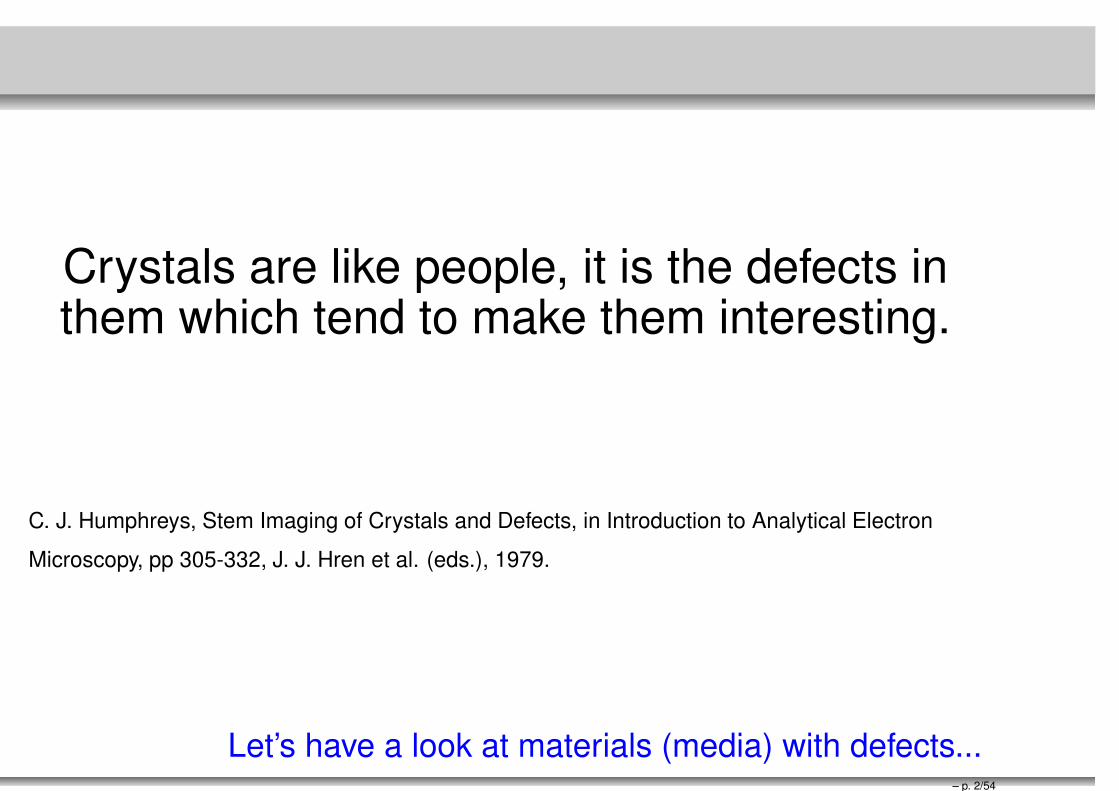
Homogenization 1.0.1: stationary ergodic setting
−div
[A(xε, ω)∇uε
]= f in D, uε = 0 on ∂D.
uε(·, ω) converges to u⋆ solution to
−div [A⋆∇u⋆] = f in D, u⋆ = 0 on ∂D, with
[A⋆]ij = E
(∫
Q
(ei +∇wei(y, ·))T A (y, ·) ej dy
),
where wp solves
−div [A (y, ω) (p+∇wp(y, ω))] = 0 in Rd, p ∈ R
d,
∇wp stat., E
(∫
Q
∇wp(y, ·) dy
)= 0.
The corrector problem is set on Rd. Theoretically, the RVE is infinite.
[Papanicolaou/Varadhan, Koslov, Bourgeat/Piatnitski, Gloria/Otto,
Armstrong/Smart, ... Caffarelli/Souganidis (nonlinear case)]
– p. 11/54

Numerical approximation
Since the corrector problem is set on Rd:
L(wp) = 0 in Rd,
∇wp is stationary
we need, in practice, to introduce truncation: introduce QN = (−N,N)d and
approximate wp by wNp with
L(wNp ) = 0 on QN ,
wNp (·, ω) is QN -periodic
and compute A⋆N (ω) from there: large domain (N ≫ 1), random output, . . .
=⇒ Often prohibitively expensive computationally!
– p. 12/54

A toolbox for modeling perturbations of a
periodic structure
– p. 13/54

Random deformations
Φ(.,ω)
A ’real’ material ≡ a random deformation of a reference periodic material
– p. 14/54

Random deformations
Deformed structure
The periodic structure corresponds to identical inclusions centered on Z2.
– p. 15/54
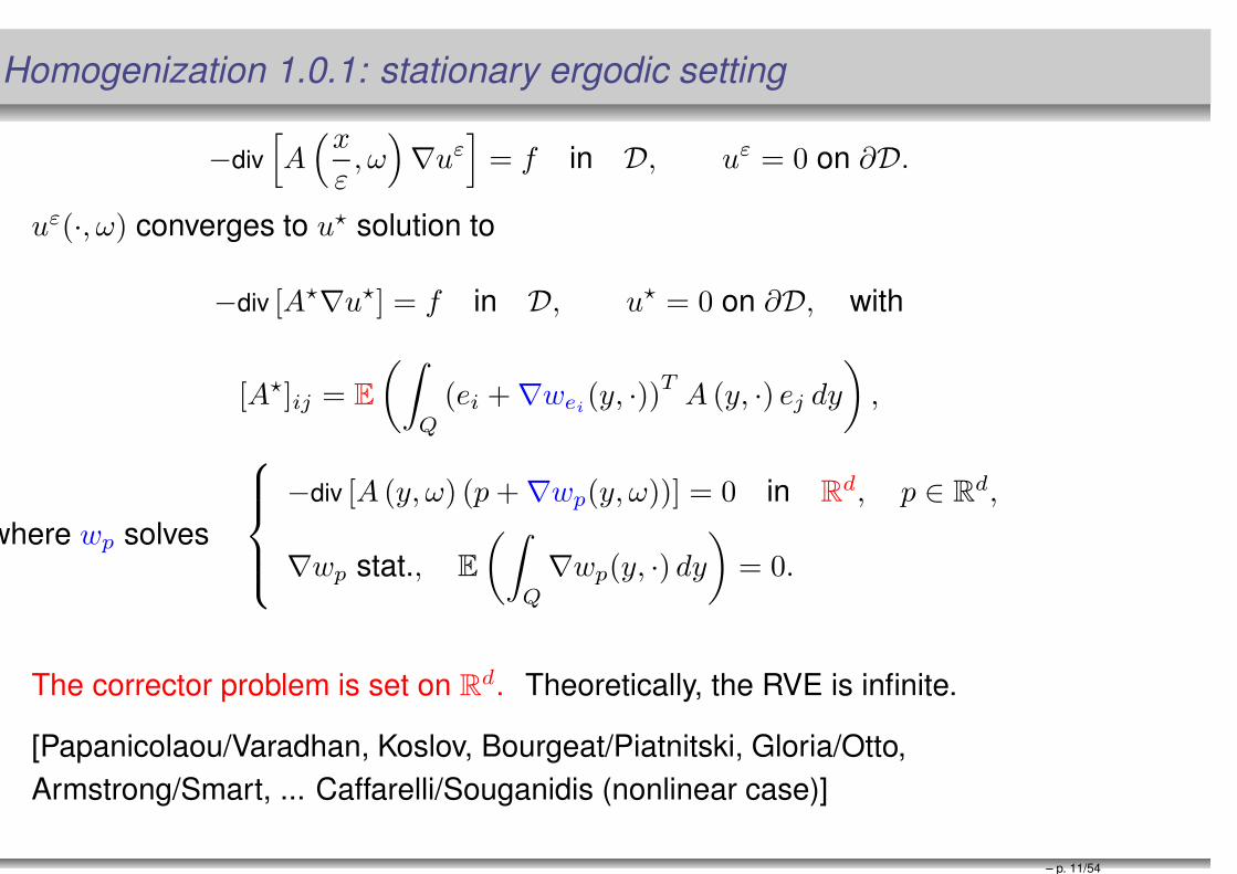
A variant of classical stochastic homogenization
Classical stochastic homogenization:
−div[A(xε, ω)∇uε(x, ω)
]= f(x) in D, uε = 0 on ∂D
where the matrix A is stationary.
We consider here a variant:
−div[Aper
(Φ−1
(xε, ω))
∇uε(x, ω)]= f(x) in D, uε = 0 on ∂D
for a periodic matrix Aper and a random diffeomorphism Φ, with ∇Φ stationary.
In general, Aper Φ−1 is NOT stationary.
Blanc/LB/Lions, C. R. Acad. Sci. (2006)
Blanc/LB/Lions, J. Math. Pures et Appliqués (2007)
(subsequently used in a variety of contexts: G. Roach et al.(2012), ... , W. Jing (2016), ... ,
T. Andrade et al. (2019), .... )
– p. 16/54

Random deformations
−div[Aper
(Φ−1
(xε, ω))
∇uε(x, ω)]= f(x) in D, uε = 0 on ∂D
uε(·, ω) converges (weakly in H1 and strongly in L2) to u⋆ almost surely, with
−div [A⋆∇u⋆(x)] = f(x) in D, u⋆ = 0 on ∂D
with the homogenized matrix
A⋆ij = det
[E
[∫
Q
∇Φ(y, ·)dy
]]−1
E
[∫
Φ(Q,·)
(ei +∇wei(y, ·))TAper
(Φ−1 (y, ·)
)ejdy
]
where, for all p ∈ Rd, wp is the corrector defined by
−div[Aper
(Φ−1(x, ω)
)(p+∇wp(x, ω))
]= 0 in R
d,
wp(x, ω) = wp(Φ−1(x, ω), ω), ∇wp is stationary,
E
(∫
Φ(Q,·)
∇wp(y, ·)dy
)= 0. ... So what?
– p. 17/54

Random (small) deformations
Assume next that the diffeomorphism Φ is close to the identity:
Φ(x, ω) = x+ ηΨ(x, ω) +O(η2),
for η small. Then
wp(x, ω) = w0p(x) + ηw1
p(x, ω) +O(η2),
with−div
(Aper
(p+∇w0
p
))= 0, w0
p is Zd-periodic,
and
−div[Aper
(∇w1
p −∇Ψ∇w0p
)+(∇ΨT − (div Ψ)Id
)Aper
(p+∇w0
p
)]= 0,
E
(∫
Q
∇w1p
)= E
(∫
Q
(∇Ψ− (div Ψ)Id)∇w0p
), ∇w1
p stationary.
– p. 18/54

Random (small) deformations
Taking the expectation and setting w1p = E(w1
p),
−div[Aper∇w1
p
]= RHS
(Aper,E(∇Ψ),∇w0
p
),
∫
Q
∇w1p =
∫
Q
(E(∇Ψ)− E(div Ψ) Id)∇w0p, ∇w1
p periodic.
Eventually,
A⋆ = A0 + ηA1 +O(η2),
with
A0ij =
∫
Q
(ei +∇w0ei)TAperej
A1ij =
∫
Q
fct[E(∇Ψ), A0,∇w0, Aper
]+
∫
Q
(∇w1ei− E(∇Ψ)∇w0
ei)TAperej .
Two periodic computations instead of an expensive stochastic one.
– p. 19/54

Randomly located defects
Define now a random “perturbation” in a different topology
A. Anantharaman/LB, C. R. Acad. Sc., 348 (2010)A. Anantharaman/LB, SIAM MMS, 9, 2 (2011)A. Anantharaman/LB, Comm. Comp. Phys., 11 (2011)
– p. 20/54

Randomly located defects
In the previous setting, we have considered aper(Φ−1(x, ω)) with
Φη(x, ω) = x+ ηΨ(x, ω) + . . . ,
and η a small scalar. We can alternately consider
Φη(x, ω) = x+ bη(x, ω)Ψ(x, ω) + . . . ,
with bη small in some suitable (random) norm.
To keep things simple, let us assume
a(x, ω) = aper(x) + bη(x, ω) cper(x).
The most interesting case is typically bη(x, ω) a Bernoulli random variable.
– p. 21/54

Randomly located defects
Remember the fibers in the composite, or the rods in the assembly...
– p. 22/54

Randomly located defects
Law of the material:
δa + η (δc − δa)
on each cell. Cells are independent from one another. Product. Expand at first order in η:
N∏
k=1
δa(cell k) + η N
[
δc(cell k = 1)N∏
k=2
δa(cell k) −N∏
k=1
δa(cell k)
]
.
Think of a jellium model in Physics, that is, a model for defects.
Next remark that in −div (A(x, ω) (p+∇w(x, ω)) = 0, the only source of randomness is in A. Put
differently, w is a deterministic function of A. Thus, we have the expansion
A∗ij =
∫ ∫
(ei +∇wei (A, y))T A(y)ejdy ρ(A) dA.
A⋆ = A0 + ηA1 + . . .
Proof of the expansion at all orders: Mourrat (JMPA, 2015), Duerinckx et al. (ARMA, 2016)
– p. 23/54

Randomly located defects
Computation of the correctors associated to all possible geometries of one, two, etc, defects. That
is, a collection of parameter-indexed elliptic PDEs.
Use of the Reduced Basis method to speed-up the computation (Y. Maday/A. Patera)
LB/Thomines, Chinese Annals of Maths. B, 33, 5 (2012)
We shall soon return to such deterministic localized defects....
– p. 24/54

Fully random homogenization problems
Of course, if the weakly random model is deemed unfit, there isthe option to address the fully random problem.
Solve the corrector problem posed on a truncated large domain,and then embrace your enemy: the noise.
A⋆ −A⋆N(ω) = A⋆ − E [A⋆
N ](small) systematic error
+ E [A⋆N ]− A⋆
N(ω)(large) statistical error
A selection of variance reduction approaches:
Costaouec/LB/Legoll, Bol. Soc. Esp. Mat. Apl., 2010.
Blanc/Costaouec/LB/Legoll, MPRF, 2012. (Antithetic Variables)
Legoll/Minvielle, DCDS-S,Vol. 8 (1), 2015. (Control Variate)
LB/Legoll/Minvielle, MCMA, 22 (1), 2016. (Special Quasi-Random Structures,
analysis by J. Fischer (ARMA, 2019))
– p. 25/54

Other equations: HJB equations
Consider the HJB equation
H(Duε, x/ε, ω) = 0
with (say) H = |p|2 − V and Vη = Vper + Vη(., ω) (Bernoulli of small
parameter η). Then
limη−→0
Hη −Hper
η
is zero for d ≥ 2 (the optimal trajectories can avoid the bumps) and is 6= 0 for
d = 1 (the trajectory necessarily hits the bump, however rare it is).
It is (currently) unclear, for d ≥ 2, what the first nontrivial term is...
Cardaliaguet/LB/Souganidis, J. Maths Pures & App., 117 (2018)
Cardaliaguet/LB/Souganidis, viscous case, work in progress.
– p. 26/54

NONPERIODICITY BY DETERMINISTIC
APPROACHES:
TOWARD A THEORY OF DEFECTS
– p. 27/54

Non stochastic problems
“General” but “explicit” deterministic problems
What is the most general property that allows homogenizationwhile keeping formulae explicit and staying deterministic?
Blanc/LB/Lions, 2002 → 2019 → ...
– p. 28/54

Non stochastic problems
Consider a set of points Xii∈N s.t.
(H1) supx∈R3
#i ∈ N / |x−Xi| < 1
< +∞,
(H2) ∃R0 > 0, infx∈R3 #i ∈ N, |x−Xi| < R0 > 0,
(H3) the following limits exist:
l0 := limR→∞
1
|BR|# i0 ∈ N, |Xi0 | ≈≤ R .
l1(h1) := limR→∞
1
|BR|#(i0, i1) ∈ N
2, |Xi0 | ≈≤ R, |Xi0 −Xi1 | ≈ h1
.
etc.
Used for Thermodynamic limit problems for interacting particle systems
(BLL, 2000’).
Next adapted to Homogenization Theory (BLL, 2010’).
– p. 29/54

General algebra
With Xi now defined, we introduce the functions
f(x) =∑
i∈N
ϕ(x−Xi), ϕ ∈ D(R3).
We consider the algebra generated by those functions and its closure for a
certain functional norm.
Examples:Compactly perturbed periodic systems: Xii∈NN = Z3 \ 0.
Ap(Xi) = Lpper(Z
3) + Lp0(R
3), (1)
where Lp0(R
3) = f ∈ Lploc(R
3), lim|x|→∞
‖f‖Lp(B+x) = 0.
Two semi-crystals:
Ap(Xi) =(
Lpper,1((Z
3)−), Lpper,2((Z
3)+))
+ Lp0(R
3).
– p. 30/54

General algebra
The question is homogenization for
−div
(a(
x
ε)∇uε
)= f,
where a is a function of the algebra, e.g.,
a(y) = 1 +∑
i∈N
ϕ(y −Xi).
Homogenization does hold, but the issue we examine is the existence of an
explicit expression for the limit.
Relation with works by G. N’Guetseng, J-L. Woukeng, et al.
– p. 31/54

General algebra
Difficulty : show that the corrector problem is well posed in thealgebra, that is , if a ∈ A then the corrector problem
−div (a(y) (p+∇wp)) = 0
is uniquely solvable for ∇wp ∈ A and < ∇wp >= 0.
The tools of elliptic problems posed on bounded domains areuseless...
At present time, no general proof, valid for an abstract generalalgebra as defined above, is known.
A variety of particular cases are considered and solved.
– p. 32/54

Well-posedness of the corrector problem
Existence of correctors for nonperiodic homogenization problems
− div (a (p+∇wp)) = 0 on Rd
Blanc/LB/Lions, Milan Journal of Maths (2012)
Blanc/LB/Lions, Comm. PDE, vol 40, 12 (2015)
Blanc/LB/Lions, Comm. PDE, Vol. 43, 6 (2019)
Blanc/LB/Lions, J. Maths P. & App., 124 (2019)
– p. 33/54

Well-posedness of the corrector problem
Consider a = aper + a where aper denotes the (unperturbed)background, and a the perturbation.
We want to solve
− div ((aper + a) (p+∇wp)) = 0
in the suitable functional class, with wp(x) = o(1 + |x|).
(a PDE problem)
– p. 34/54

Well-posedness of the corrector problem
Case considered: perturbation of a periodic background aper, thatis a = aper + a. We would like to address the case
a(x)|x|→∞−→ 0, but are only able to treat
a ∈ Lr(Rd), for some 1 ≤ r < +∞.
Second case (not considered today): twin-boundaries, that is twodifferent periodic structures separated by a flat interface.
aper(x) = aper,1,2(x) =
aper,1(x) when x1 ≤ 0,
aper,2(x) when x1 > 0,
(plus possibly a perturbation a on top of that).
– p. 35/54
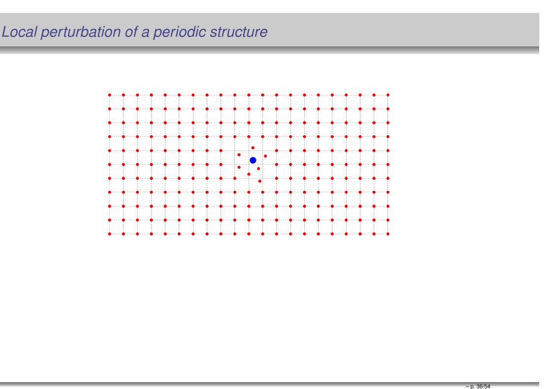
Local perturbation of a periodic structure
– p. 36/54

"Generic" Bi-crystal: "Twin boundaries"
– p. 37/54

A theoretical ingredient for MsFEM
Coarse mesh with a P1 Finite Element basis functions φ0i .
MsFEM basis
−div(Aε(x)∇φε,Ki ) = 0 in K
φε,Ki = φ0
i
∣∣K
on ∂K
and glue them together: φεi such that φε
i |K = φε,Ki for all K. The MsFEM
functions are computed independently (in parallel) over each K.
Solve the macro problem with MsFEM basis functions φεi .
Efendiev, Hou, Allaire, Peterseim, ...
– p. 38/54

Numerical illustration
Relative errors using the periodic (left) and the adapted corrector (right).
∥
∥
∥∇uε (ε ·)−∇uε,1
per (ε ·)∥
∥
∥
L2(Ω)
‖∇uε (ε ·)‖L2(Ω)
,
−div ((aper(x/ε)+a(x/ε))∇uε) = f.
Blanc/LB/Lions, Milan Journal of Maths, 2012.
– p. 39/54

Defect a ∈ Lr(Rd), r 6= 2
Theorem [Blanc/LB/Lions, Comm. PDE, 2015.]
(Lr-perturbation of periodic): Assume periodicity of thebackground and Hölder regularity. Then, the corrector problemhas a unique solution wp, up to the addition of a constant.Moreover, wp = wp,per + wp, where wp,per is the periodic correctorand
if 1 ≤ r < d, then, lim|x|→+∞
wp(x) = 0 ;
if 2 ≤ r, then ∇wp ∈ Lr.
Remarks: Periodicity of aper and Hölder regularity of aper and a areneeded. The case r = d is clearly critical.
– p. 40/54

More general proof [Blanc/LB/Lions, Comm. PDE, 2019]
Once the corrector equation is written under the form
− div (a∇wp) = div (a (p+∇wp,per)) ,
it is immediate to see that proving the existence/uniqueness ofthe corrector amounts to establishing the estimate
− div (a∇u) = div (f) ⇒ ‖∇u‖Lq(Rd) ≤ Cq ‖f‖Lq(Rd)
for the coefficient a = aper + a and a ∈ Lr(Rd). (Apply to q = r).
We indeed show that such an estimate holds true, usingconcentration-compactness to reduce the problem to the periodicresult of [Avellaneda-Lin]. And we do so in a variety of settings ...
– p. 41/54

Approximation theory
Approximation theory for nonperiodic homogenization problems
"The corrector corrects"
wε = w(·/ε) =⇒ rates of convergence
Blanc/Josien/LB, C. R. Acad. Sc, vol. 357, 2 (2019)Blanc/Josien/LB, Asymptotic Analysis, to appear.
– p. 42/54
Approximation theory for nonperiodic homogenization
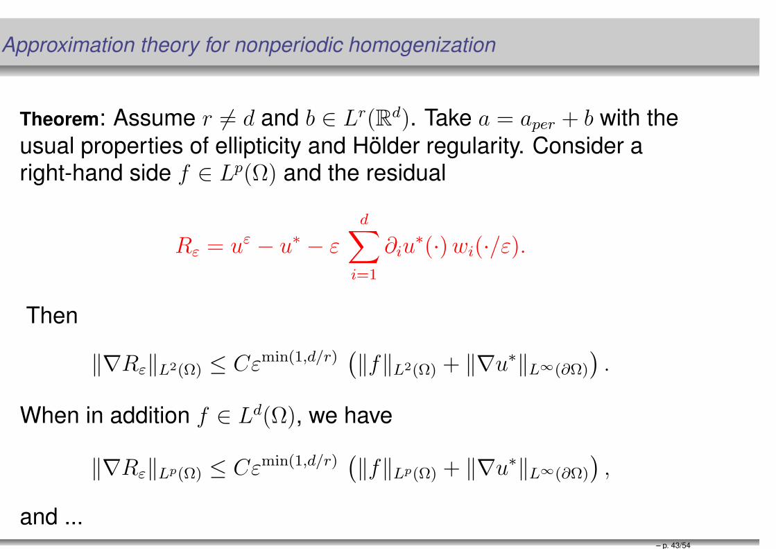
Theorem: Assume r 6= d and b ∈ Lr(Rd). Take a = aper + b with the
usual properties of ellipticity and Hölder regularity. Consider aright-hand side f ∈ Lp(Ω) and the residual
Rε = uε − u∗ − εd∑
i=1
∂iu∗(·)wi(·/ε).
Then
‖∇Rε‖L2(Ω) ≤ Cεmin(1,d/r)(‖f‖L2(Ω) + ‖∇u∗‖L∞(∂Ω)
).
When in addition f ∈ Ld(Ω), we have
‖∇Rε‖Lp(Ω) ≤ Cεmin(1,d/r)(‖f‖Lp(Ω) + ‖∇u∗‖L∞(∂Ω)
),
and ...– p. 43/54

Approximation theory for nonperiodic homogenization
1
B(0, ε)
∫
B(0,ε)
|∇Rε|2 ≤ Cεmin(1,d/r)−d/p
(‖f‖Lp(Ω) + ‖∇u∗‖L∞(∂Ω)
).
If d ≥ 3 and f is Hölder regular, then
‖∇Rε‖L∞(Ω) ≤ Cεmin(1,d/r)(1 + | ln ε−1|
)‖f‖C0,β(Ω).
The point for the proof is wε = w(·/ε).
– p. 44/54

Approximation theory for nonperiodic homogenization
The proof follows the same pattern as those by Avellaneda/Linand Kenig/Lin/Shen in the periodic case. It concatenates
1. Lε converges to L∗ thus "what is true for the latter is true forthe former when ε is small"
2. estimate of the Green function Gε(x, y) by Grüter/Widman(only ellipticity)
3. estimate of its derivative ∂xGε(x, y) and ∂x∂yGε(x, y) (structure
is needed)
4. estimate of the rate of convergence of Rε following for aregular right-hand side
5. argument by duality for the convergence of the Greenfunctions Gε(x, y)− G∗(x, y)
– p. 45/54

Extensions
interface problems, M. Josien (CPDE, 2019)
perforated domains, X. Blanc/S. Wolf (subm., 2019)
defects "rare" at infinity, Blanc/Goudey/LB, work in progress
...
nonlinear problems, ...
– p. 46/54
Other equations
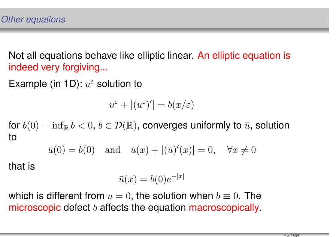
Not all equations behave like elliptic linear. An elliptic equation isindeed very forgiving...
Example (in 1D): uε solution to
uε + |(uε)′| = b(x/ε)
for b(0) = infR b < 0, b ∈ D(R), converges uniformly to u, solutionto
u(0) = b(0) and u(x) + |(u)′(x)| = 0, ∀x 6= 0
that is
u(x) = b(0)e−|x|
which is different from u = 0, the solution when b ≡ 0. Themicroscopic defect b affects the equation macroscopically.
– p. 47/54

Best constant matrix
Coarse approximation of an oscillatory elliptic problem
"Homogenization with partial information"
LB/ Legoll/ Li, C. R. Acad. Sc., 351, (2013)LB/ Legoll/Lemaire, ESAIM: COCV, vol 24, Issue 4 (2018)Gorynina/LB/Legoll, in preparation.
– p. 48/54

Best constant matrix
There exist many practical situations in
−div (Aε∇uε) = f in Ω ⊂ Rd, for which
Aε is not entirely known: one can only measure / observe the
solution uε for some loadings f (think of mechanical experiments),
so we have no access to the corrector equation.
homogenization theory does not give explicit formulae for A⋆
even if explicit, A⋆ is challenging to compute (or even as difficult as
Aε, like in the fractal case)
Can we nevertheless approximate Aε by a constant matrix, e.g.
bypassing the computation of the correctors to compute A⋆, or the
computation of local problems in a dedicated Galerkin procedure?
– p. 49/54
Best constant matrix
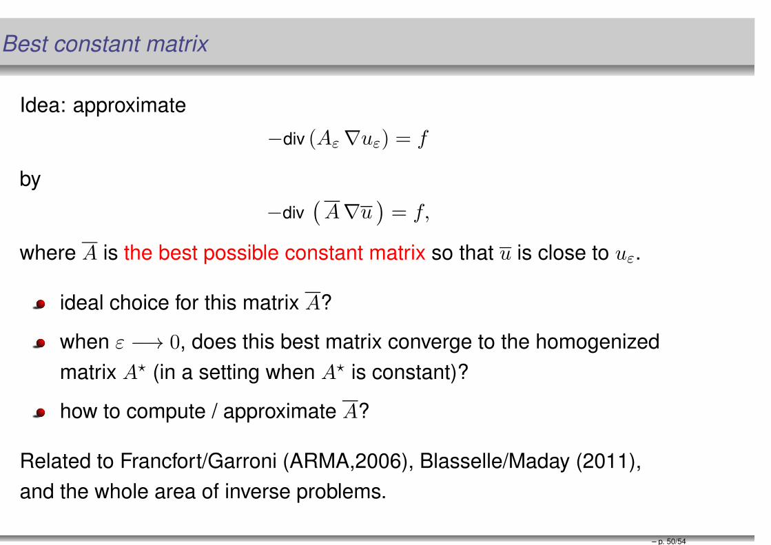
Idea: approximate
−div (Aε∇uε) = f
by
−div(A∇u
)= f,
where A is the best possible constant matrix so that u is close to uε.
ideal choice for this matrix A?
when ε −→ 0, does this best matrix converge to the homogenized
matrix A⋆ (in a setting when A⋆ is constant)?
how to compute / approximate A?
Related to Francfort/Garroni (ARMA,2006), Blasselle/Maday (2011),
and the whole area of inverse problems.
– p. 50/54

Best constant matrix
Iε = infconstant matrix A > 0
supf∈L2(Ω), ‖f‖
L2(Ω)=1
∥∥uε(f)− u(A, f
)∥∥2L2(Ω)
︸ ︷︷ ︸Jε(A)
Then
limε→0
Iε = 0.
for any quasi-minimizing matrix Aε (i.e. Iε ≤ Jε(Aε
)≤ Iε + ε), we
have limε→0
Aε = A⋆.
Ingredients of the proof:
knowing RA =(−divA∇
)−1amounts to knowing A when A is a
constant matrix (in fact ‖RA −RB‖ ≈ ‖A−B‖)
the definition of Iε guarantees the convergence of RAεto RA⋆ , thus
that of Aε to A⋆.– p. 51/54

Best constant matrix
Formally, we wish to consider
Iε = infconstant matrix A > 0
supf∈L2(Ω), ‖f‖
L2(Ω)=1
∥∥uε(f)− u(A, f
)∥∥2L2(Ω)
.
Following an idea by Albert Cohen, we instead consider (compose by
the 0-order operator ∆−1 divA∇)
Iε = infconstant matrix A > 0
supf∈L2(Ω), ‖f‖
L2(Ω)=1
∥∥−∆−1(−divA∇uε(f)− f
)∥∥2L2(Ω)
Same theoretical result as above. Practically: much better because
quadratic functional in A and more robust!
– p. 52/54

Best constant matrix
in practice, supf is replaced by max(f1,...,fN ) ⊕ strategy to
choose the sample set of suitable r.h.s. fi
the corrector function is obtained by a post-process, usingthe two-scale expansion as a proxy
the approach carries over to random homogenization
an interesting variant introduced by R. Cottereau (IJNME,2013): use the Arlequin coupling method (in order to avoidboundary effects) along with an optimization loop to identifythe homogenized tensor (improved in Gorynina/LB/Legoll,work in progress).
– p. 53/54

Thanks to:
Pierre-Louis Lions,Panagiotis Souganidis, Pierre Cardaliaguet,Xavier Blanc, Frédéric Legoll,Alexei Lozinski, Ulrich Hetmaniuk,Olga Gorynina, Rémi Goudey, Sylvain Wolf,
and to many colleagues for stimulating and enlightening discussions:
Ludovic Chamoin (ENS Saclay), Albert Cohen (Sorbonne), RégisCottereau (CNRS Marseille), Yalchin Efendiev (TAMU), RalfKornhuber (FUB), Mitchell Luskin (UMN), ...
Support from ONR and EOARD is gratefully acknowledged.
– p. 54/54