Homogenization and dimension reduction of filtration combustion in heterogeneous thin ... ·...
32
Homogenization and dimension reduction of filtration combustion in heterogeneous thin layers Fatima, T.; Ijioma, E.R.; Ogawa, T.; Muntean, A. Published: 01/01/2014 Document Version Publisher’s PDF, also known as Version of Record (includes final page, issue and volume numbers) Please check the document version of this publication: • A submitted manuscript is the author's version of the article upon submission and before peer-review. There can be important differences between the submitted version and the official published version of record. People interested in the research are advised to contact the author for the final version of the publication, or visit the DOI to the publisher's website. • The final author version and the galley proof are versions of the publication after peer review. • The final published version features the final layout of the paper including the volume, issue and page numbers. Link to publication Citation for published version (APA): Fatima, T., Ijioma, E. R., Ogawa, T., & Muntean, A. (2014). Homogenization and dimension reduction of filtration combustion in heterogeneous thin layers. (CASA-report; Vol. 1402). Eindhoven: Technische Universiteit Eindhoven. General rights Copyright and moral rights for the publications made accessible in the public portal are retained by the authors and/or other copyright owners and it is a condition of accessing publications that users recognise and abide by the legal requirements associated with these rights. • Users may download and print one copy of any publication from the public portal for the purpose of private study or research. • You may not further distribute the material or use it for any profit-making activity or commercial gain • You may freely distribute the URL identifying the publication in the public portal ? Take down policy If you believe that this document breaches copyright please contact us providing details, and we will remove access to the work immediately and investigate your claim. Download date: 02. Jun. 2018
Transcript of Homogenization and dimension reduction of filtration combustion in heterogeneous thin ... ·...
Homogenization and dimension reduction of filtrationcombustion in heterogeneous thin layersFatima, T.; Ijioma, E.R.; Ogawa, T.; Muntean, A.
Published: 01/01/2014
Document VersionPublisher’s PDF, also known as Version of Record (includes final page, issue and volume numbers)
Please check the document version of this publication:
• A submitted manuscript is the author's version of the article upon submission and before peer-review. There can be important differencesbetween the submitted version and the official published version of record. People interested in the research are advised to contact theauthor for the final version of the publication, or visit the DOI to the publisher's website.• The final author version and the galley proof are versions of the publication after peer review.• The final published version features the final layout of the paper including the volume, issue and page numbers.
Link to publication
Citation for published version (APA):Fatima, T., Ijioma, E. R., Ogawa, T., & Muntean, A. (2014). Homogenization and dimension reduction of filtrationcombustion in heterogeneous thin layers. (CASA-report; Vol. 1402). Eindhoven: Technische UniversiteitEindhoven.
General rightsCopyright and moral rights for the publications made accessible in the public portal are retained by the authors and/or other copyright ownersand it is a condition of accessing publications that users recognise and abide by the legal requirements associated with these rights.
• Users may download and print one copy of any publication from the public portal for the purpose of private study or research. • You may not further distribute the material or use it for any profit-making activity or commercial gain • You may freely distribute the URL identifying the publication in the public portal ?
Take down policyIf you believe that this document breaches copyright please contact us providing details, and we will remove access to the work immediatelyand investigate your claim.
Download date: 02. Jun. 2018

EINDHOVEN UNIVERSITY OF TECHNOLOGY Department of Mathematics and Computer Science
CASA-Report 14-02 February 2014
Homogenization and dimension reduction of filtration combustion in heterogeneous thin layers
by
T. Fatima, E.R. Ijioma, T. Ogawa, A. Muntean
Centre for Analysis, Scientific computing and Applications
Department of Mathematics and Computer Science
Eindhoven University of Technology
P.O. Box 513
5600 MB Eindhoven, The Netherlands
ISSN: 0926-4507

HOMOGENIZATION AND DIMENSION REDUCTION OF
FILTRATION COMBUSTION IN HETEROGENEOUS THIN
LAYERS
Tasnim Fatima1
Department of Mathematics and Computer Science
CASA - Center for Analysis, Scientific computing and Applications
Eindhoven University of TechnologyP.O. Box 513, 5600 MB, Eindhoven, The Netherlands
Ekeoma Ijioma2 Toshiyuki Ogawa
Graduate School of Advanced Mathematical ScienceMeiji University
4-21-1 Nakano, Nakano-ku, Tokyo, 164-8525, Japan
Adrian Muntean
Department of Mathematics and Computer Science
CASA - Center for Analysis, Scientific computing and Applications
ICMS - Institute for Complex Molecular SystemsEindhoven University of Technology
P.O. Box 513, 5600 MB, Eindhoven, The Netherlands
Abstract. We study the homogenization of a reaction-diffusion-convection
system posed in an ε-periodic δ-thin layer made of a two-component (solid-air)composite material. The microscopic system includes heat flow, diffusion and
convection coupled with a nonlinear surface chemical reaction. We treat two
distinct asymptotic scenarios: (1) For a fixed width δ > 0 of the thin layer,we homogenize the presence of the microstructures (the classical periodic ho-
mogenization limit ε→ 0); (2) In the homogenized problem, we pass to δ → 0
(the vanishing limit of the layer’s width). In this way, we are preparing thestage for the simultaneous homogenization (ε → 0) and dimension reductionlimit (δ → 0) with δ = δ(ε). We recover the reduced macroscopic equations
from [21] with precise formulas for the effective transport and reaction coeffi-cients. We complement the analytical results with a few simulations of a case
study in smoldering combustion. The chosen multiscale scenario is relevant
for a large variety of practical applications ranging from the forecast of theresponse to fire of refractory concrete, the microstructure design of resistance-
to-heat ceramic-based materials for engines, to the smoldering combustion ofthin porous samples under microgravity conditions.
2000 Mathematics Subject Classification. Primary: 35B27; Secondary: 76S05; 74E30; 80A25;35B25; 35B40.
Key words and phrases. Homogenization, dimension reduction, thin layers, filtration combus-
tion, two-scale convergence, anisotropic singular perturbations.1T. Fatima is a visitor of CASA.2Corresponding author.
1
2 T. FATIMA E. R. IJIOMA T. OGAWA AND A. MUNTEAN
1. Introduction.
1.1. Aim of the paper. We wish to investigate the sub-sequential homogenizationand dimension reduction limits for a reaction-diffusion-convection system coupledwith a non-linear differential equation posed in a periodically-distributed array ofmicrostructures; see [21, 20] for details on the smoldering combustion context in-spiring this paper. To prove the homogenization limit we rely on the two-scaleconvergence (cf. e.g. [6, 26, 15]). Relying on the estimates obtained in this paper,we hope to deal at a later stage with the boundary layers occurring during thesimultaneous homogenization-dimension reduction procedure. We expect that theconcept of two-scale convergence for thin heterogeneous layers [29] and appropriatescaling arguments, somewhat similar to the spirit of [4, 7] are applicable. A similarstrategy would be to use a periodic unfolding operator depending on two parame-ters [11]. It is worth noting that the simultaneous homogenization and dimensionreduction limit is a relevant research topic related to the rigorous derivation of platetheories, and away from the elasticity framework; see e.g. [16, 1, 27] and referencescited therein.
This paper prepares a framework where such a simultaneous limit can be donefor a filtration combustion scenario.
1.2. Mathematical background. Homogenization of problems depending on twoor more small parameters is a useful averaging tool when dealing for instance withreticulated structures (see e.g. [12]) or with porous media with thin fractures (seee.g. [4]). Often in such cases, the small parameters correspond to scale-separatedprocesses and can therefore be treated as being independent of each other. Themost challenging mathematical situation is when the two small parameters are inter-related, i.e. δ = δ(ε) where ε > 0 takes into account the periodicity scale (or thelength scale of a reference elementary volume) and δ > 0 a typical length scaleof the microstructure. This kind of scaling dependence δ = δ(ε) with δ > ε > 0makes such setting resemble a boundary layer case. Essentially, due to the lackof scale separation, one can easily imagine that when passing to δ → 0 one loosesthe information at the ε-scale; like for instance, in the balance in measures settingdiscussed in [34].
1.3. Estimating the heat response of materials with microstructure. Ho-mogenization of heat transfer scenarios has attracted the attention of many re-searchers in the last years; see for instance the references indicated in [39, 26, 3]as well as in the doctoral thesis by Habibi [17] (where the focus is on the radiativetransfer of heat). For a closely related multiscale setting where convection interplayswith diffusion and chemistry, we refer the reader to the elementary presentation ofthe main issues given in [37]. For a computational approach to heat conduction inmultiscale solids, see [33].
The practical application we have in mind includes the multiscale modeling ofreverse smoldering combustion, aiming at understanding the behavior of fingeringpatterns arising from a controlled experimental study of smoldering combustionof thin porous samples under microgravity conditions. The details of such an ex-perimental scenario have been reported previously in [41, 32], and treated math-ematically in different contexts [22, 14, 25, 40]. In all these papers, the modelsare introduced directly at the macroscopic scale and less attention is paid on thechoice of microstructures as well as to the influence of physical processes at the porescale. Our paper wishes to fill some gaps in this direction. There are also other

FILTRATION COMBUSTION IN HETEROGENEOUS THIN LAYERS 3
related studies [35, 31] dealing with averaging of combustion processes. Closely re-lated application areas include the design of microstructures for refractory concrete– a composite heterogeneous material with special chemical composition (meant topostpone de-hydratation [36]), also referred to as blast furnance. The refractoryconcrete materials are expected to sustain high temperatures and moderate convec-tion, typical of situations arising in the furnance of steel factories; for more detailssee [5] and references cited therein.
1.4. Organization of the material. We proceed as follows: We first ensure thesolvability of the microscopic combustion model. Then we check how the modelresponds to the application of the two-scale convergence as ε → 0 for the caseδ = O(1) recovering in this way the structure of the averaged model equationsobtained in [21] by means of formal asymptotics homogenization. Then as nextstep, the limit δ → 0 turns to be a regular perturbation scenario that we approachwith techniques inspired by the averaging of reticulated geometries; see [12]. Usingthe macroscopic equations obtained in the case ε → 0 for δ → 0, we illustratenumerically the instability of combustion fingers as observed experimentally in [41].Finally, we conclude the paper with a brief enumeration of a couple of open problemsarising from this filtration combustion scenario.
1.5. Contents of the paper. The paper is organized in the following fashion:
Contents
1. Introduction 21.1. Aim of the paper 21.2. Mathematical background 21.3. Estimating the heat response of materials with microstructure 21.4. Organization of the material 31.5. Contents of the paper 32. Notations. Assumptions on geometry. Unknowns 33. Setting of the microscopic equations - the model (Pδε) 54. Solvability of the (Pδε)-model 64.1. Working hypotheses 64.2. Basic estimates and results 75. The homogenization limit ε→ 0. The case δ > ε > 0, δ = O(1). 165.1. Extensions to Ωδ 165.2. Two-scale convergence step 175.3. Derivation of upscaled limit equations 186. The dimension reduction limit δ → 0 217. Numerical illustration of the fingering instability. The case δ > ε > 0, δ = O(1). 248. Discussion 25Acknowledgments 26
REFERENCES26
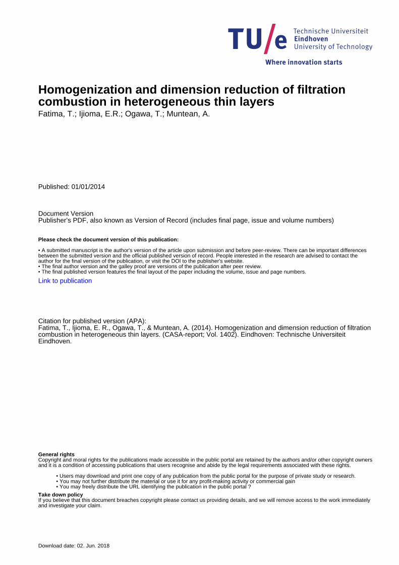
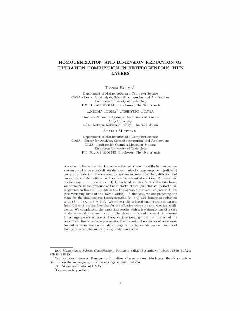
2. Notations. Assumptions on geometry. Unknowns. The geometry of theporous material we have in mind is depicted in Figure 2. It is basically obtainedby replicating and then glueing periodically the unit cell/pore structure depicted inFigure 1.
4 T. FATIMA E. R. IJIOMA T. OGAWA AND A. MUNTEAN
Yg
Ys
Figure 1. δ-cell (ball microscopic fabric).
x1
x2
x3
Figure 2. Periodically-distributed array of cells contained in aε-thin layer.
Yg
Ys
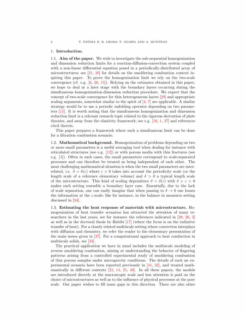
Figure 3. δ-cell (parallelipiped microscopic fabric).
x1
x2
x3
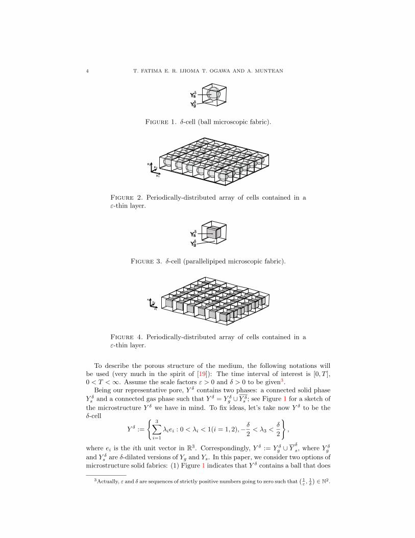
Figure 4. Periodically-distributed array of cells contained in aε-thin layer.
To describe the porous structure of the medium, the following notations willbe used (very much in the spirit of [19]): The time interval of interest is [0, T ],0 < T <∞. Assume the scale factors ε > 0 and δ > 0 to be given3.
Being our representative pore, Y δ contains two phases: a connected solid phase
Y δs and a connected gas phase such that Y δ = Y δg ∪ Y δs ; see Figure 1 for a sketch of
the microstructure Y δ we have in mind. To fix ideas, let’s take now Y δ to be theδ-cell
Y δ :=
3∑i=1
λiei : 0 < λi < 1(i = 1, 2),−δ2< λ3 <
δ
2
,
where ei is the ith unit vector in R3. Correspondingly, Y δ := Y δg ∪ Yδ
s, where Y δgand Y δs are δ-dilated versions of Yg and Ys. In this paper, we consider two options ofmicrostructure solid fabrics: (1) Figure 1 indicates that Y δ contains a ball that does
3Actually, ε and δ are sequences of strictly positive numbers going to zero such that(1ε, 1δ
)∈ N2.

FILTRATION COMBUSTION IN HETEROGENEOUS THIN LAYERS 5
not touch ∂Y δ, and (2) Figure 3 indicates that Y δ contains a (solid) parallelepipedthat does not touch ∂Y δ.
For subsets X of Y δ and integer vectors k = (k1, k2, k3) ∈ Z3 we denote thee1, e2-directional shifted subset by
Xk := X +
2∑i=1
kiei.
The geometry within our layer Ωδ includes the pore skeleton Ωδεs and the porespace Ωδεg . Obviously, we have
Ωδ := Ωδεg ∪ Ωδε
s
with
Γδε := ∂Ωδεsas the (total) gas-solid boundary. As indicated in the Figures above, the microstruc-tures are not allowed to touch neither themselves nor the outer boundary of the layerΩδ.
Finally, note that
∂Ωδ = ΓδD ∪ ΓδN ∪ Γδε,
that is the boundary of the layer Ωδ can be split into the exterior Dirichlet andNeumann boundaries (ΓδD and ΓδN ) and the inner gas-solid boundary Γδε.
On the other hand, w.l.o.g. assume that we can take Ω a bounded domain in R2
as side for the layer Ωδ such that Ωδ := Ω × [−δ2,δ
2]. Later on in section 6, when
taking δ → 0 we will understand that Ωδ → Ω×0 (the dimension reduction step)with Y δ → Y × 0, where Ω, Y ⊂ R2. We will write for the reduced homogenizedproblem Ω, Y , etc. instead of Ω × 0 and Y × 0 and so on. Also, denote
Ω := Ω×[− 1
2 ,12
].
By χΘ we denote the characteristic function of the set Θ. Typical choices for theset Θ will be Y δg , Y
δs , etc.
Given uδε : Ωδεg → R3 velocity of the flow, the unknowns of the microscopic model
are: Cδε : Ωδεg → R – the concentration of the active species (typically oxygen),
T δεg : Ωδεg → R and T δεs : Ωδεs → R – the temperatures corresponding to the solid
and gas phases of the material, and Rδε : Γδε → R – the solid reaction product.For the sake of a simpler notation, for the case δ = O(1), we omit to write the
dependence of the solution vector (Cδε, T δε, Rδε) [with T δε := (T δεg , T δεs )] on thescale factor δ; we just write (Cε, T ε, Rε) but still keep the presence of δ in thedefinition of the space domain.
3. Setting of the microscopic equations - the model (Pδε). We investigatethe model equations proposed in [21] to describe the smoldering combustion of aporous medium and pose it now in the thin layer Ωδ (see Figure 2 or Figure 4) asfollows: Find the triplet (Cδε, T δε, Rδε) satisfying
∂tCδε +∇ · (uδεCδε −Dδε∇Cδε) = 0 in Ωδεg ,
Cδεg ∂tTδεg +∇ · (Cδεg uδεT δεg − λδεg ∇T δεg ) = 0 in Ωδεg ,
Cδεs ∂tTδεs −∇ · (λδεs ∇T δεs ) = 0 in Ωδεs ,
∂tRδε = W (T δε, Cδε) on Γδε,
(1)

6 T. FATIMA E. R. IJIOMA T. OGAWA AND A. MUNTEAN
together with initial and boundary conditions
Cδε(0, x) = C0 in t = 0 × ΩδεgT δεi (0, x) = T 0
i in t = 0 × Ωδεi , i ∈ g, sRδε(0, x) = R0 on t = 0 × Γδε
(λδεg ∇T δεg − λδεs ∇T δεs ) · ν = εQW (T δε, Cδε) on Γδε,
T δεg = T δεs on Γδε,
Dδε∇Cδε · ν = −εW (T δε, Cδε) on Γδε,
(2)and
T δεi = Tu, Cδε = Cu on ΓδD∇T δεi · ν = 0, ∇Cδε · ν = 0 on ΓδN .
(3)
We denote the production term by surface combustion reaction by W (T δε, Cδε) :=ACδεf(T δε). We refer to this microscopic model as the (Pδε)-model.
4. Solvability of the (Pδε)-model.
4.1. Working hypotheses. Before performing any asymptotics, we wish to ensurethat the microscopic model (Pδε) is well-posed. To do so, we introduce a set ofrestrictions on data and parameters, which we collect as Assumptions (A).
We assume the following set of assumptions, to which we refer to as Assump-tions (A):
(A1) Dδ, λδg, λδs ∈ L∞(Y δ)3×3, (Dδ(x)ξ, ξ) ≥ D0|ξ|2 for D0 > 0, (λδg(x)ξ, ξ) ≥
λ0g|ξ|2 for λ0
g > 0, (λδs(x)ξ, ξ) ≥ λ0s|ξ|2 for λ0
s > 0 and every ξ ∈ R3, y ∈ Y δ.(A2) f is bounded and Lipschitz function. Furthermore
f(α) =
positive, if α > 0,
0, otherwise.
(A3) Cδεg , Cδεs are bounded from below by C0
g , C0s , respectively.
(A4) C0, C0g , C
0s ∈ H1(Ωδ)∩L∞+ (Ωδ), R ∈ L∞+ (Γδ). C0, T 0
g , T0s ∈ H1(Ωδ)∩L∞+ (Ωδ)
and R ∈ L∞+ (Γδ).
(A5) ‖uδε‖L2([0,T ]×Ωδ) ≤Mu <∞ and uδε → uδ strongly as ε→ 0.
(A6) Cu, Tu ∈ H1(0, T ;H1(Ωδεg )) ∩ L∞+ ((0, T )× Ωδεg ).
We also define the following uniform in δ constants
MC := ‖C0‖L∞(Ωδ), (4)
MT := max‖T 0g ‖L∞(Ωδ), ‖T 0
s ‖L∞(Ωδ),MR := max‖R0‖L∞(Γδ),MT .
Definition 4.1. We call (Cδε, T δεg , T δεs , Rδε) a weak solution to (1)–(2) if Cδε ∈Cu+L2(0, T ;H1
Γ(Ωδεg )), ∂tCδε ∈ ∂tCu+L2(0, T ;L2(Ωδεg )), T δεg ∈ Tu+L2(0, T ;H1
Γ(Ωδεg )),
∂tTδεg ∈ ∂tTg +L2(0, T ;L2(Ωδεg )), T δεs ∈ L2(0, T ;H1(Ωδεs ))∩H1(0, T ;L2(Ωδεs )), and

FILTRATION COMBUSTION IN HETEROGENEOUS THIN LAYERS 7
Rδε ∈ H1(0, T ;L2(Γδε)) satisfies a.e. in (0, T ) the following formulation∫Ωδεg
∂tCδεφdx+
∫Ωδεg
Dδε∇Cδε∇φdx+
∫Ωδεg
uδε∇Cδεφdx = −ε∫
Γδε
W (T δε, Cδε)φdγ,
∫Ωδεg
Cδεg ∂tTδεg ϕdx+
∫Ωδεg
λδεg ∇T δεg ∇ϕdx+
∫Ωδεg
Cδεg uδε∇T δεg ϕdx+
∫Ωδεs
Cδεs ∂tTδεs ϕdx
∫Ωδεs
λδεs ∇T δεs ∇ϕdx = ε
∫Γδε
QW (T δε, Cδε)ϕdγ,
∫Γδε
∂tRδεψdγ =
∫Γδε
W (T δε, Cδε)ψdγ,
for all φ ∈ L2(0, T ;H1Γ(Ωδεg )), ϕ ∈ L2(0, T ;H1
Γ(Ωδεg )) × L2(0, T ;H1(Ωδεs )), ψ ∈L2((0, T )×Γδε) and Cδε(t)→ C0, T δεg (t)→ T 0
g in L2(Ωδεg ), T δεs (t)→ T 0g in L2(Ωδεs ),
Rδε(t)→ R0 in L2(Γδε) as t→ 0.
4.2. Basic estimates and results.
Lemma 4.2. (Energy estimates) Assume (A1)–(A4), then the weak solution to themicroscopic problem (Pδε) in the sense of Definition 4.1 satisfies the following apriori estimates
‖ Cδεg ‖L2(0,T ;L2(Ωδεg )) + ‖ ∇Cδεg ‖L2(0,T ;L2(Ωδεg ))≤ C, (5)
‖ T δεi ‖L2(0,T ;L2(Ωδεi )) + ‖ ∇Cδεi ‖L2(0,T ;L2(Ωδεi ))≤ C, for i ∈ g, s (6)√ε ‖ Rδε ‖L∞((0,T )×Γδε) +
√ε ‖ ∂tRδε ‖L2((0,T )×Γδε)≤ C (7)
Proof. We test with φ = Cδε to get
t∫0
∫Ωδεg
∂t|Cδε|2dxdτ + 2D0
t∫0
∫Ωδεg
|∇Cδε|2dxdτ +
t∫0
∫Ωδεg
uδε · ∇CδεCδεdxdτ
≤ 2εA
∫Γδε
|Cδε|2f(T δε)dγdτ.
Convection term in (8) vanishes. This follows from
t∫0
∫Ωδεg
uδε∇CδεCδεdxdτ =1
2
t∫0
∫Ωδεg
uδε∇|Cδε|2dxdτ
=1
2
t∫0
∫Γδε
n.uδε|Cδε|2dxdτ − 1
2
t∫0
∫Ωδεg
∇ · uδε|Cδε|2dxdτ.
Using the boundedness of f , the fact that uδε is divergence-free and zero on theboundary and the trace inequality, we obtain
t∫0
∫Ωδεg
∂t|Cδε(t)|2dxdτ + (2D0 − ε2C)
t∫0
∫Ωδεg
|∇Cδε|2dxdτ ≤ Ct∫
0
∫Ωδεg
|Cδε(t)|2dxdτ.

8 T. FATIMA E. R. IJIOMA T. OGAWA AND A. MUNTEAN
Choosing ε small enough and applying Gronwall’s inequality, we obtain the desiredresult. Let us take φ = (T δεg , T δεs ) ∈ L2(0, T ;H1
Γ(Ωδεg ))× L2(0, T ;H1(Ωδεs )) to get
C0g
t∫0
∫Ωδεg
∂t|T δεg |2dxdτ + 2λ0g
t∫0
∫Ωδεg
|∇T δεg |2dxdτ + C0g
t∫0
∫Ωδεg
uδε∇|T δεg |2dxdτ
+C0s
t∫0
∫Ωδεs
∂t|T δεs |2dxdτ + 2λ0s
t∫0
∫Ωδεs
|∇T δεs |2dxdτ
≤ 2εAQ
t∫0
∫Γδε
f(T δε)CδεT δεdγdτ ≤ εCt∫
0
∫Γδε
CδεT δεdγdτ. (8)
The convection term disappears by the argument given above. Furthermore, weestimate the integral on right hand side as follows:
εC
t∫0
∫Γδε
CδεT δεdγdτ ≤ εCt∫
0
∫Γδε
(|Cδε|2 + |T δε|2)dγdτ
≤ C
t∫0
∫Ωδεg
(|Cδε|2 + ε2|∇Cδε|2 + |T δεg |2 + ε2|∇T δεg |2
)dxdτ
+C
t∫0
∫Ωδεs
(|T δεs |2 + ε2|∇T δεs |2
)dxdτ.
(8) becomes
C0g
t∫0
∫Ωδεg
∂t|T δεg |2dxdτ + (2λ0g − ε2C)
t∫0
∫Ωδεg
|∇T δεg |2dxdτ
+C0s
t∫0
∫Ωδεs
∂t|T δεs |2dxdτ + (2λ0s − ε2C)
t∫0
∫Ωδεs
|∇T δεs |2dxdτ
≤ Ct∫
0
∫Ωδεg
(|Cδε|2 + ε2|∇Cδε|2 + |T δεg |2
)dxdτ + C
t∫0
∫Ωδεs
|T δεs |2dxdτ.
Choosing ε conveniently, using estimates (5) and applying Gronwall’s inequality, weget
∫Ωδεi
|T δεi (t)|2dx+
t∫0
∫Ωδεi
|∇T δεi |2dxdτ ≤ C i ∈ g, s.

FILTRATION COMBUSTION IN HETEROGENEOUS THIN LAYERS 9
We set as a test function ψ = Rδε and get
ε
t∫0
∫Γδε
∂t|Rδε|2dγdτ = 2εA
t∫0
∫Γδε
f(T δε)CδεRδεdγdτ
≤ εC
t∫0
∫Γδε
(|Cδε|2 + |Rδε|2
)dγdτ.
Applying Gronwall’s inequality together with trace inequality, we have
ε
∫Γδε
|Rδε(t)|2dγ ≤ C
t∫0
∫Ωδεg
(|Cδε|2 + ε2|∇Cδε|2
)dx
Using (5), we have the result. Now we take as a test function ψ = ∂tRδε and obtain
ε
t∫0
∫Γδε
|∂tRδε|2dγdτ = εA
t∫0
∫Γδε
f(T δε)Cδε∂tRδεdγdτ
≤ εA
t∫0
∫Γδε
( 1
2ξ|Cδε|2 +
ξ
2|∂tRδε|2
)dγdτ
ε(1− Aξ
2)
t∫0
∫Γδε
|∂tRδε|2dγdτ ≤ A
2ξ
t∫0
∫Ωδεg
(|Cδε|2 + ε2|∇Cδε|2
)dx.
Choosing ξ conveniently and using (5) to obtain
√ε ‖ ∂tRδε ‖L2((0,T )×Γδε)≤ C.
Lemma 4.3. (Positivity) Assume (A1)-(A4), and let t ∈ [0, T ] be arbitrarily cho-sen. Then the following estimates hold:
(i) Cδε(t), T δεg (t) ≥ 0 a.e. in Ωδεg , T δεs (t) ≥ 0 a.e. in Ωδεs and Rδε(t) ≥ 0 a.e. on
Γδε.(ii) Cδε(t) ≤ MC , T δεg (t) ≤ MT a.e. in Ωδεg , T δεs (t) ≤ MT a.e. in Ωδεs and
Rδε(t) ≤MR a.e. on Γδε, where MC , MT and MR are defined in 4.
Proof. (i) We test with φ = −[Cδε]− and obtain the following inequality
1
2
t∫0
∫Ωδεg
∂t|[Cδε]−|2dxdτ +D0
t∫0
∫Ωδεg
|∇[Cδε]−|2dxdτ +
t∫0
∫Ωδεg
uδε∇Cδε[Cδε]−dxdτ
≤ εA
t∫0
∫Γδε
|[Cδε]−|2dγdτ. (9)
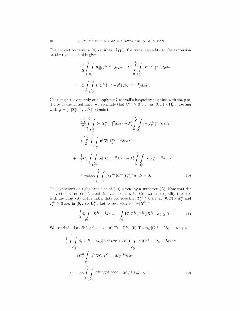
10 T. FATIMA E. R. IJIOMA T. OGAWA AND A. MUNTEAN
The convection term in (9) vanishes. Apply the trace inequality to the expressionon the right hand side gives
1
2
t∫0
∫Ωδεg
∂t|[Cδε]−|2dxdτ +D0
t∫0
∫Ωδεg
|∇[Cδε]−|2dxdτ
≤ C
t∫0
∫Ωδεg
(|[Cδε]−|2 + ε2|∇[Cδε]−|2
)dxdτ.
Choosing ε conveniently and applying Gronwall’s inequality together with the pos-itivity of the initial data, we conclude that Cδε ≥ 0 a.e. in (0, T ) × Ωδεg . Testing
with ϕ = (−[T δεg ]−, [T δεs ]−) leads to
C0g
2
t∫0
∫Ωδεg
∂t|[T δεg ]−|2dxdτ + λ0g
t∫0
∫Ωδεg
|∇[T δεg ]−|2dxdτ
+C0g
2
t∫0
∫Ωδεg
uε∇|[T δεg ]−|2dxdτ
+1
2C0s
t∫0
∫Ωδεs
∂t|[T δεs ]−|2dxdτ + λ0s
t∫0
∫Ωδεs
|∇[T δεs ]−|2dxdτ
≤ −εQAt∫
0
∫Γδε
f(T δε)Cδε[T δεg ]−dγdτ ≤ 0. (10)
The expression on right hand side of (10) is zero by assumption (A). Note that theconvection term on left hand side vanishe as well. Gronwall’s inequality togetherwith the positivity of the initial data provides that T δεg ≥ 0 a.e. in (0, T )×Ωδεg and
T δεs ≥ 0 a.e. in (0, T )× Ωδεs . Let us test with ψ = −[Rδε]−
1
2∂t
∫Γδε
|[Rδε]−|2dγ = −∫
Γδε
W (T δε, Cδε)[Rδε]−dγ ≤ 0. (11)
We conclude that Rδε ≥ 0 a.e. on (0, T )× Γδε. (ii) Taking [Cδε −MC ]+, we get
1
2
t∫0
∫Ωδεg
∂t|[Cδε −MC ]+|2dxdτ +D0
t∫0
∫Ωδεg
|∇[Cδε −MC ]+|2dxdτ
+C0g
∫Ωδεg
uδε∇C [εC
δε −MC ]+dxdτ
≤ −εAt∫
0
∫Γδε
Cδεf(T ε)[Cδε −MC ]+dγdτ ≤ 0. (12)

FILTRATION COMBUSTION IN HETEROGENEOUS THIN LAYERS 11
Arguing as before, we observe that the convection term vanishes. Applying Gron-wall’s inequality together with C0 ≤ MC a.e. in Ωδεg , we end up with the bound-
edness of the Cδε ≤ MC a.e. in Ωδεg for all t ∈ (0, T ). Note that since Cδε ∈L2(0, T ;H1
Γ(Ωδεg ))∩L∞((0, T )×Ωδεg ), by Claim 5 in [15] we have Cδε ∈ L∞((0, T )×Γδε). Testing with ([T δεg −MT ]+, [T δεs −MT ]+) and the resulting inequalities
C0g
2
t∫0
∫Ωδεg
∂t|[T δεg −MT ]+|2dxdτ +C0s
2
t∫0
∂t
∫Ωδεs
|[T δεs −MT ]+|2dxdτ
+ λ0g
t∫0
∫Ωδεg
|∇[T δεg −MT ]+|2dxdτ + λ0s
t∫0
∫Ωδεs
|∇[T δεs −MT ]+|2dxdτ
+1
2
t∫0
∫Ωδεg
uδε∇|[T δεg −MT ]+|2dxd ≤ εQAt∫
0
∫Γδε
f(T δε)Cδε[T δε −MT ]+dγdτ
≤ εQAMc
t∫0
∫Γδε
|[T δε −MT ]+|2dγdτ. (13)
Using boundedness of Cδε on Γδε and the sublinearity of f and, then, applying traceinequality, leads to
t∫0
∫Ωδεg
∂t|[T δεg −MT ]+|2dxdτ +
t∫0
∫Ωδεs
∂t|[T δεs −MT ]+|2dxdτ
+(2λ0
g
C0g
− Cε2)
t∫0
∫Ωεg
|∇[T δεg −MT ]+|2dxdτ
+(2λ0
s
C2s
− Cε2)
t∫0
∫Ωδεs
|∇[T δεs −MT ]+|2dxdτ
≤ Ct∫
0
∫Ωδεg
|[T δεg −MT ]+|2dxdτ + C
t∫0
∫Ωδεs
|[T δεs −MT ]+|2dxdτ.
Let us choose ε small enough. Applying again Gronwall’s inequality, we obtainT δεg ≤ MT a.e. in Ωδεg and T δεs ≤ MT a.e. in Ωδεs . Now we test with [Rδε − (t +
1)MR]+ and obtain∫Γδε
(∂t|[Rδε − (t+ 1)MR]+|2 +MR[Rδε − (t+ 1)MR]+
)dγ
≤ C∫
Γδε
Mc[Rδε − (t+ 1)MR]+dγ
∫Γδε
∂t|[Rδε − (t+ 1)MR]+|2dγ ≤ (CMc −MR)
∫Γδε
[Rδε − (t+ 1)MR]+dγ
12 T. FATIMA E. R. IJIOMA T. OGAWA AND A. MUNTEAN
Using (A5) and Gronwall’s inequality to get Rδε ≤MR a.e. in (0, T )× Γδε.
Remark 1. Based on Cδε ∈ L∞((0, T )×Ωδεg )∩L2(0, T ;H1(Ωδεg )), we use Claim 5
in [15] to obtain Cδε ∈ L∞((0, T )× Γδε).
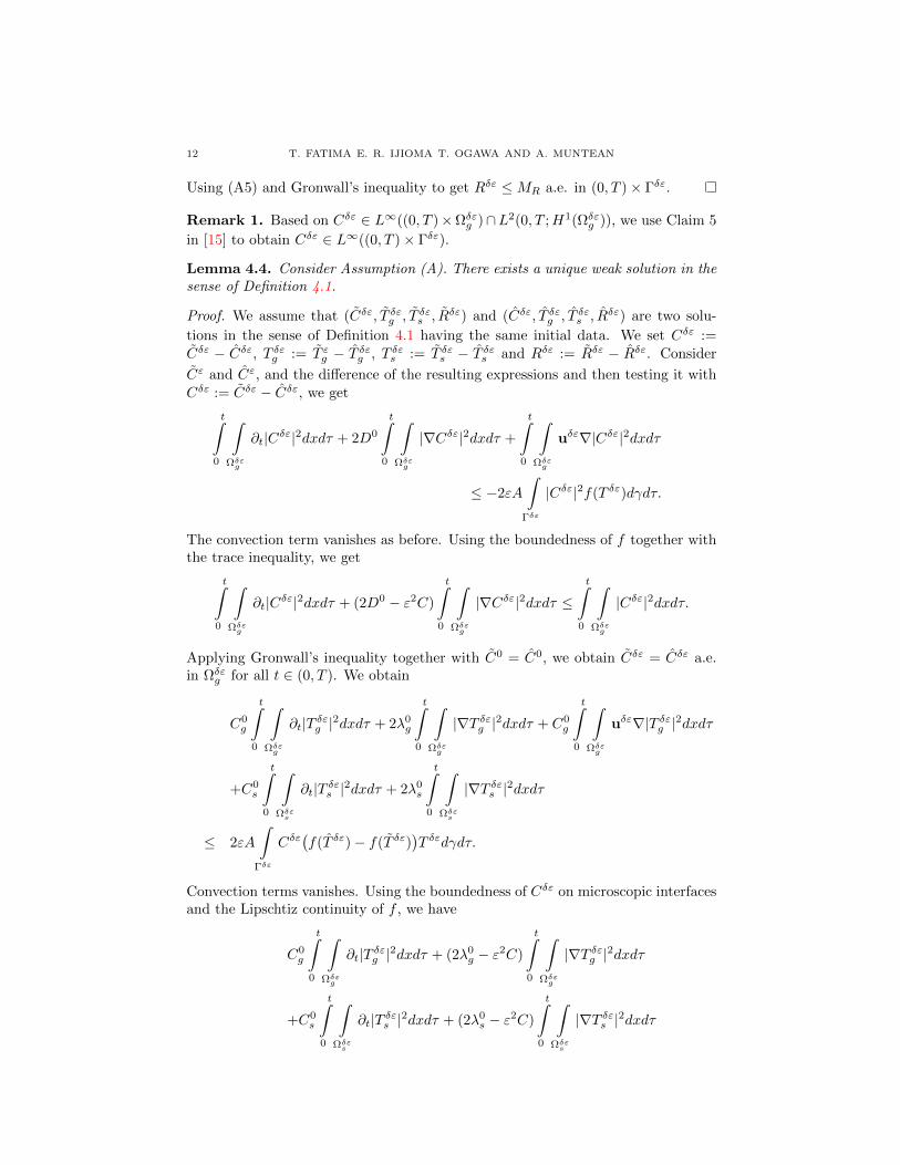
Lemma 4.4. Consider Assumption (A). There exists a unique weak solution in thesense of Definition 4.1.
Proof. We assume that (Cδε, T δεg , T δεs , Rδε) and (Cδε, T δεg , T δεs , Rδε) are two solu-
tions in the sense of Definition 4.1 having the same initial data. We set Cδε :=Cδε − Cδε, T δεg := T εg − T δεg , T δεs := T δεs − T δεs and Rδε := Rδε − Rδε. Consider
Cε and Cε, and the difference of the resulting expressions and then testing it withCδε := Cδε − Cδε, we get
t∫0
∫Ωδεg
∂t|Cδε|2dxdτ + 2D0
t∫0
∫Ωδεg
|∇Cδε|2dxdτ +
t∫0
∫Ωδεg
uδε∇|Cδε|2dxdτ
≤ −2εA
∫Γδε
|Cδε|2f(T δε)dγdτ.
The convection term vanishes as before. Using the boundedness of f together withthe trace inequality, we get
t∫0
∫Ωδεg
∂t|Cδε|2dxdτ + (2D0 − ε2C)
t∫0
∫Ωδεg
|∇Cδε|2dxdτ ≤t∫
0
∫Ωδεg
|Cδε|2dxdτ.
Applying Gronwall’s inequality together with C0 = C0, we obtain Cδε = Cδε a.e.in Ωδεg for all t ∈ (0, T ). We obtain
C0g
t∫0
∫Ωδεg
∂t|T δεg |2dxdτ + 2λ0g
t∫0
∫Ωδεg
|∇T δεg |2dxdτ + C0g
t∫0
∫Ωδεg
uδε∇|T δεg |2dxdτ
+C0s
t∫0
∫Ωδεs
∂t|T δεs |2dxdτ + 2λ0s
t∫0
∫Ωδεs
|∇T δεs |2dxdτ
≤ 2εA
∫Γδε
Cδε(f(T δε)− f(T δε)
)T δεdγdτ.
Convection terms vanishes. Using the boundedness of Cδε on microscopic interfacesand the Lipschtiz continuity of f , we have
C0g
t∫0
∫Ωδεg
∂t|T δεg |2dxdτ + (2λ0g − ε2C)
t∫0
∫Ωδεg
|∇T δεg |2dxdτ
+C0s
t∫0
∫Ωδεs
∂t|T δεs |2dxdτ + (2λ0s − ε2C)
t∫0
∫Ωδεs
|∇T δεs |2dxdτ
FILTRATION COMBUSTION IN HETEROGENEOUS THIN LAYERS 13
≤ C
∫Ωδεg
|T δεg |2dxdτ + C
∫Ωδεs
|T δεs |2dxdτ.
choosing ε conveniently, applying Gronwall’s inequality and taking supremum alongt ∈ [0, T ], we obtain the following estimate
C0g
∫Ωδεg
|T δεg |2dx+ C
T∫0
∫Ωδεg
|∇T δεg |2dxdτ
+C0s
∫Ωδεs
|T δεs |2dx+ C
T∫0
∫Ωδεs
|∇T δεs |2dxdτ ≤ 0.
Hence, we conclude that T δεi = T δεi , i ∈ g, s a.e. t ∈ (0, T ) in Ωδεi . The uniquenessof Rδε is a natural consequence of the uniqueness of T δε and Cδε.
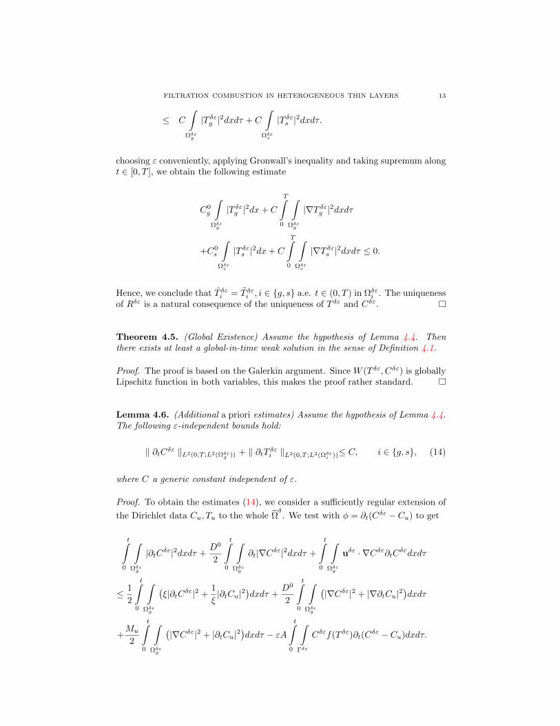
Theorem 4.5. (Global Existence) Assume the hypothesis of Lemma 4.4. Thenthere exists at least a global-in-time weak solution in the sense of Definition 4.1.
Proof. The proof is based on the Galerkin argument. Since W (T δε, Cδε) is globallyLipschitz function in both variables, this makes the proof rather standard.
Lemma 4.6. (Additional a priori estimates) Assume the hypothesis of Lemma 4.4.The following ε-independent bounds hold:
‖ ∂tCδε ‖L2(0,T ;L2(Ωδεg )) + ‖ ∂tT δεi ‖L2(0,T ;L2(Ωδεi ))≤ C, i ∈ g, s, (14)
where C a generic constant independent of ε.
Proof. To obtain the estimates (14), we consider a sufficiently regular extension of
the Dirichlet data Cu, Tu to the whole Ωδ. We test with φ = ∂t(C
δε − Cu) to get
t∫0
∫Ωδεg
|∂tCδε|2dxdτ +D0
2
t∫0
∫Ωδεg
∂t|∇Cδε|2dxdτ +
t∫0
∫Ωδεg
uδε · ∇Cδε∂tCδεdxdτ
≤ 1
2
t∫0
∫Ωδεg
(ξ|∂tCδε|2 +
1
ξ|∂tCu|2
)dxdτ +
D0
2
t∫0
∫Ωδεg
(|∇Cδε|2 + |∇∂tCu|2
)dxdτ
+Mu
2
t∫0
∫Ωδεg
(|∇Cδε|2 + |∂tCu|2
)dxdτ − εA
t∫0
∫Γδε
Cδεf(T δε)∂t(Cδε − Cu)dxdτ.
14 T. FATIMA E. R. IJIOMA T. OGAWA AND A. MUNTEAN
(1− Cξ
2)
t∫0
∫Ωδεg
|∂tCδε|2dxdτ +D0
2
∫Ωδεg
|∇Cδε(t)|2dx
≤ D0
2
∫Ωδεg
|∇Cδε(0)|2dx+1
2ξ
t∫0
∫Ωδεg
|∂tCu|2dxdτ
+D0
2
t∫0
∫Ωδεg
(|∇Cδε|2 + |∇∂tCu|2
)dxdτ +
Mu
2δ
t∫0
∫Ωδεg
|∇Cδε|2dxdτ
+Mu
2
t∫0
∫Ωδεg
(|∇Cδε|2 + |∂tCu|2
)dxdτ
+ εC
t∫0
∫Γδε
(∂t|Cδε|2 + |Cδε|2 + |∂tCu|2
)dxdτ.
(1− Cξ
2)
t∫0
∫Ωδεg
|∂tCδε|2dxdτ +D0
2
∫Ωδεg
|∇Cδε(t)|2dx
≤ D0
2
∫Ωδεg
|∇Cδε(0)|2dx+ C
t∫0
∫Ωδεg
(|∇Cδε|2 + |∇∂tCu|2 + |∂tCu|2
)dxdτ
+ C
∫Ωδεg
(|Cδε(t)|2 + ε2|∇Cδε(t)|2 + |Cδε(0)|2 + ε2|∇Cδε(0)|2
)dx
+ C
t∫0
∫Ωδεg
(|Cδε|2 + ε2|∇Cδε|2 + |∂tCu|2 + ε|∇∂tCu|2
)dxdτ.
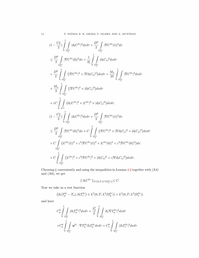
Choosing ξ conveniently and using the inequalities in Lemma 4.2 together with (A4)and (A6), we get
‖ ∂tCδε ‖L2(0,T ;L2(Ωδεg ))≤ C.
Now we take as a test function(∂t(T
δεg − Tu), ∂tT
δεs
)∈ L2(0, T ;L2(Ωδεg ))× L2(0, T ;L2(Ωδεs ))
and have
C0g
t∫0
∫Ωδεg
|∂tT δεg |2dxdτ +λ0g
2
t∫0
∫Ωδεg
∂t|∇T δεg |2dxdτ
+C0g
t∫0
∫Ωδεg
uδε · ∇T δεg ∂tTδεg dxdτ + C0
s
t∫0
∫Ωδεs
|∂tT δεs |2dxdτ

FILTRATION COMBUSTION IN HETEROGENEOUS THIN LAYERS 15
+λ0s
2
t∫0
∫Ωδεs
∂t|∇T δεs |2dxdτ
≤t∫
0
∫Ωδεg
λδεg ∇T δεg ∇∂tTudxdτ +
t∫0
∫Ωδεg
Cδεg ∂tTδεg ∂tTudxdτ
+C0g
t∫0
∫Ωδεg
uδε · ∇T δεg ∂tTudxdτ + εQA
t∫0
∫Γδε
Cδεf(T δε)∂tTδεdxdτ
C0g
t∫0
∫Ωδεg
|∂tT δεg |2dxdτ +λ0g
2
∫Ωδεg
|∇T δεg (t)|2dx
+C0s
t∫0
∫Ωδεs
|∂tT δεs |2dxdτ +λ0s
2
∫Ωδεs
|∇T δεs (t)|2dx
≤λ0g
2
∫Ωδεg
|∇T δεg (0)|2dx+λ0s
2
∫Ωδεs
|∇T δεs (0)|2dx
+Mu
2
t∫0
∫Ωδεg
(1
ξ|∇T δεg |2 + ξ|∂tT δεg |2
)dxdτ
+C0g
2
t∫0
∫Ωδεg
(δ|∂tT δεg |2 +
1
ξ|∂tTu|2
)dxdτ
+C
t∫0
∫Ωδεg
(|∇T δεg |2 + |∂tTu|2 + |∇∂tTu|2
)dxdτ
+εC
t∫0
∫Γδε
∂t|T δε|2dγdτ
Making use of the boundedness of Cδε on (0, T )× Γδε and of the sub-linearity of f
(C0g −
Muξ
2)
t∫0
∫Ωδεg
|∂tT δεg |2dxdτ +λ0g
2
∫Ωδεg
|∇T δεg (t)|2dx
+C0s
t∫0
∫Ωδεs
|∂tT δεs |2dxdτ +λ0s
2
∫Ωδεs
|∇T δεs (t)|2dx
≤λ0g
2
∫Ωδεg
|∇T δεg (0)|2dx+λ0s
2
∫Ωδεs
|∇T δεs (0)|2dx
16 T. FATIMA E. R. IJIOMA T. OGAWA AND A. MUNTEAN
+C
t∫0
∫Ωδεg
(|∇T δεg |2 + |∂tT δεg |2 + |∇∂tT δεg |2
)dxdτ
+C
∫Ωδεs
(|T δεs (t)|2 + ε2|∇T δεs (t)|2 + |T δεs (0)|2 + ε2|∇T δεs (0)|2)dx.
Choosing ξ conveniently and using the inequalities in Lemma 4.2 together with(A4), we get
‖ ∂tT δεg ‖L2(0,T ;L2(Ωδεg )) + ‖ ∂tT δεs ‖L2(0,T ;L2(Ωδεs ))≤ C. (15)
Remark 2. We can use the Cauchy-Schwarz inequality together with (15) to showthe boundedness from above of the microscopic instantaneous bulk burning rate
V δε(t) :=
∫Ω
|∂tT δε(t, x)|1δdx (16)
as well as its time average
< V δε(t) >t:=1
t
∫ t
0
V δε(s)ds (17)
with
T δε(x, t) :=
T δεg (x, t), if x ∈ ΩδεgT δεs (x, t), if x ∈ Ωδεs ,
for any t ∈ (0, T ). We refer the reader to [13] for the terminology and use of suchbulk burning rates.
5. The homogenization limit ε→ 0. The case δ > ε > 0, δ = O(1).
5.1. Extensions to Ωδ. Our main interest lies in the passing to the homogenizationlimit ε→ 0. Before passing to this limit, we extend all the unknowns of the problemto the whole space Ωε. Using a standard extension result due to D. Cioranescu andJ. Saint Jean Paulin [10], we extend the concentration defined in Ωεg inside the solidgrains; see also Lemma 2.4 in [26] for a related result. The temperature extendsnaturally in the whole domain by taking the extended temperature field
T ε(x, t) :=
T εg (x, t), if x ∈ ΩεgT εs (x, t), if x ∈ Ωεs.
Since the nonlinearity imposed at the microstructure boundary turns to be globallyactually Lipschitz, there are no problems in stating the existence of the extendedtemperature field. We refer the reader to [23] for a situation where, due to thepresence of (boundary) multivalued functions, a more detailed investigation of theexistence of the extension is needed. If more effects are introduced at the microscopicsolid-gas interfaces like temperature jumps, or heating delays (etc), effects thatcould require the introduction of a second temperature (see e.g. [14, 26]), then theextension step requires a special care.

FILTRATION COMBUSTION IN HETEROGENEOUS THIN LAYERS 17
5.2. Two-scale convergence step.
Definition 5.1. (Two-scale convergence; cf. [2, 30]) Let uε be a sequence offunctions in L2((0, T )× Ω) (Ω being an open set of RN ) where ε being a sequenceof strictly positive numbers tends to zero. uε is said to two-scale converge to aunique function u0(t, x, y) ∈ L2((0, T )×Ω×Y ) if and only if for any ψ ∈ C∞0 ((0, T )×Ω, C∞# (Y )), we have
limε→0
∫ T
0
∫Ω
uε(t, x)ψ(t, x,x
ε)dxdt =
1
|Y |
∫Ω
∫Y
u0(t, x, y)ψ(t, x, y)dydxdt. (18)
We denote (18) by uε2 u0.
Theorem 5.2. (Two-scale compactness on volumes; cf. [2, 30])
(i) From each bounded sequence uε in L2((0, T )×Ω), one can extract a subse-quence which two-scale converges to u0(t, x, y) ∈ L2((0, T )× Ω× Y ).
(ii) Let uε be a bounded sequence in H1((0, T ) × Ω), then there exists u ∈L2((0, T ) × Ω;H1
#(Y )/R) such that up to a subsequence uε two-scale con-
verges to u0(t, x) ∈ L2((0, T )× Ω) and ∇uε 2 ∇xu0 +∇yu.
Definition 5.3. (Two-scale convergence for ε−periodic hypersurfaces; cf. [28]) Asequence of functions uε in L2((0, T )×Γε) is said to two-scale converge to a limitu0 ∈ L2((0, T )× Ω× Γ) if and only if for any ψ ∈ C∞0 ((0, T )× Ω, C∞# (Γ)) we have
limε→0ε
∫ T
0
∫Γε
uε(t, x)ψ(t, x,x
ε)dσxdt =
1
|Y |
∫Ω
∫Γ
u0(t, x, y)ψ(t, x, y)dσydxdt.
Theorem 5.4. (Two-scale compactness on hypersurfaces; cf. [28])
(i) From each bounded sequence uε ∈ L2((0, T )× Γε), one can extract a subse-quence uε which two-scale converges to a function u0 ∈ L2((0, T )× Ω× Γ).
(ii) If a sequence of functions uε is bounded in L∞((0, T )×Γε), then uε two-scaleconverges to a function u0 ∈ L∞((0, T )× Ω× Γ).
The estimates stated in Lemma 4.2 and Lemma 4.6 ensure the following conver-gence results:
Lemma 5.5. Assume (A1)–(A6). Then, for any fixed δ > 0, we have as ε→ 0 thefollowing convergences (up to subsequences):
(a) Cδε, T δε Cδ, T δ weakly in L2(0, T ;H1(Ωδ),
(b) Cδε, T δε∗ Cδ, T δ weakly in L∞((0, T )× Ωδ),
(c) ∂tCδε, ∂tT
δε ∂tCδ, ∂tT
δ weakly in L2((0, T )× Ωδ),(d) Cδε, T δε strongly in L2(0, T ;Hβ(Ωδ)) for 1
2 < β < 1,
also√ε ‖ Cδε−Cδ ‖L2((0,T )×Γδε)→ 0 and
√ε ‖ T δε−T δ ‖L2((0,T )×Γδε)→ 0 as
ε→ 0.(e) Cδε, T δε
2 Cδ, T δ,∇Cδε 2
∇xCδ+∇yCδ, Cδ ∈ L2((0, T )×Ωδ;H1#(Y δg )/R),
∇T δε 2 ∇xT δ +∇yT δ, T δ ∈ L2((0, T )× Ωδ;H1
#(Y δ)/R),
(f) Rδε2 Rδ, and Rδ ∈ L∞((0, T )× Ωδ × Γδ),
(g) ∂tCδε, ∂tT
δε 2 ∂tC
δ, ∂tTδ, and ∂tR
δε 2 ∂tR
δ ∈ L2((0, T )× Ωδ × Γδ).
Proof. (a) and (b) are obtained as a direct consequence of the fact that Cδε, T δε arebounded in L2(0, T ;H1(Ωδ))∩L∞((0, T )×Ωδ). Up to a subsequence (still denotedby Cδε, T ε), Cδε, T δε converge weakly to Cδ, T δ in L2(0, T ;H1(Ωδ)) ∩ L∞((0, T )×
18 T. FATIMA E. R. IJIOMA T. OGAWA AND A. MUNTEAN
Ωδ). A similar argument gives (c). To get (d), we use the compact embedding
Hβ′(Ωδ) → Hβ(Ωδ), for β ∈ ( 1
2 , 1) and 0 < β < β′ ≤ 1 (since Ωδ has Lips-
chitz boundary). We have W := Cδε, T δε ∈ L2(0, T ;H1(Ωδ)) and ∂tCδε, ∂tT
δε ∈L2((0, T )× Ωδ). For a fixed ε, W is compactly embedded in L2(0, T ;Hβ(Ωδ)) bythe Lions-Aubin Lemma; cf. e.g. [24]. Using the trace inequality for oscillatingsurfaces
√ε ‖ Cδε − Cδ ‖L2((0,T )×Γδε) ≤ C ‖ Cδε − Cδ ‖L2(0,T ;Hβ(Ωδεg ))
≤ C ‖ Cδε − Cδ ‖L2(0,T ;Hβ(Ωδ))
where ‖ Cδε −Cδ ‖L2(0,T ;Hβ(Ωδ))→ 0 as ε→ 0. Similar argument holds for the restof (d). To investigate (e), (f) and (g), we use the notion of two-scale convergence asindicated in Definition 5.1 and 5.3. Since Cδε are bounded in L2(0, T ;H1(Ωδ)), up
to a subsequence Cδε2 Cδ in L2((0, T )× Ωδ), and ∇Cδε 2
∇xCδ +∇yCδ, Cδ ∈L2((0, T ) × Ωδ;H1
#(Y δg )/R). By Theorem 5.4, Rδε in L∞((0, T ) × Γδε) converges
two-scale to Rδ ∈ L∞((0, T ) × Ωδ × Γδ) and ∂tRδε converges two-scale to ∂tR
δ inL2((0, T )× Ωδ × Γδ).
5.3. Derivation of upscaled limit equations. To be able to formulate the limit(upscaled) equations in a compact manner, we define two classes of cell problems(local auxiliary problems) very much in the spirit of [18].
Definition 5.6. The cell problems for the gaseous part are given by−∇y.(D(y)∇yωk) =
∑3i=1 ∂ykDki(y) in Y δg ,
−D(y)∂ωk
∂n =∑3i=1Dki(y)ni on Γδ,
(19)
for all k ∈ 1, 2, 3 and ωk are Y δ-periodic in y.−∇y.(λg(y)∇yωkg ) =
∑3i=1 ∂ykλgki(y) in Y δg ,
−λg(y)∂ωkg∂n =
∑3i=1 λgki(y)ni on Γδ,
(20)
for all k ∈ 1, 2, 3 and ωkg are Y δ-periodic in y. The cell problems for the solid partare given by
−∇y.(λs(y)∇yωks ) =∑3i=1 ∂ykλski(y) in Y δs ,
−dλs(y)∂ωks∂n =
∑3i=1 λski(y)ni on Γδ
(21)
for all k ∈ 1, 2, 3, ωks are Y δ-periodic in y.
Standard theory of linear elliptic problems with periodic boundary conditionsensures the weak solvability of the families of cell problems (19) – (21); see e.g. Ref.[9].
The main result of this section is the following:
Theorem 5.7. The sequence of weak solutions of the microscopic problem (in thesense of Definition (4.1)) converges as ε→ 0 to the triplet (Cδ, T δ, Rδ), where Cδ ∈Cu+L2(0, T ;H1
Γ(Ωδ)), ∂tCδ ∈ ∂tCu+L2(0, T ;L2(Ωδ)), T δ ∈ Tu+L2(0, T ;H1
Γ(Ωδ)),∂tT
δ ∈ ∂tTu + L2(0, T ;L2(Ωδ)), and Rδ ∈ H1(0, T ;L2(Ωδ × Γδ)) satisfying weaklythe following macroscopic equations a.e. in Ωδ for all t ∈ (0, T )
∂tCδ +∇ · (−D∇Cδ + uδCδ) = − |Γ
δ||Y δg |
W (T δ, Cδ), (22)

FILTRATION COMBUSTION IN HETEROGENEOUS THIN LAYERS 19
C∂tTδ +∇ · (−L∇T δ+ < Cg >Y δg uδT δ) =
|Γδ||Y δ|
QW (T δ, Cδ), (23)
∂t < Rδ >Γδ= W (T δ, Cδ), (24)
where
< Rδ >Γδ (t, x) :=1
|Γδ|
∫ΓδRδ(t, x, y)dγ
and
< Cg >Y δg :=1
|Y δg |
∫Y δg
Cg(y)dy
for all x ∈ Ωδ and all t ∈ (0, T ). Furthermore, the effective heat capacity C, theeffective diffusion tensor D, and the effective heat conduction tensor L are given by
C :=
∫Y δ
[Cg(y)χY δg (y) + Cs(y)χY δg (y)]dy (25)
(D)jk :=1
|Y δg |
3∑`=1
∫Y δg
(D)jk + (D)`k∂y`ωj)dy (26)
(L)jk := (Λg)jk + (Λg)jk (27)
(Λg)jk :=
3∑`=1
∫Y δ
((λg)jk + (λg)`k∂y`ωjg)χY δg (y)dy
(Λs)jk :=
3∑`=1
∫Y δ
((λs)jk + (λs)`k∂y`ωjs)χY δs (y)dy
with ωj , ωji being solutions of the cell problems defined in Definition 5.6. Herei ∈ g, s and j, k ∈ 1, 2, 3. The initial values
Cδ(0, x) = C0(x), T δg (0, x) = T 0(x) for x ∈ Ωδ
Rδ(0, x, y) = R0(x, y) for (x, y) ∈ Ωδ × Γδ,
together with the boundary conditions
Cδ = Cu on ΓδD, (28)
−D∇Cδ · ν = 0 on ΓδN , (29)
T δ = Tu on ΓδD, (30)
−L∇T δ · ν = 0 on ΓδN . (31)
complete the formulation of the macroscopic problem.Furthermore, it exists at most one triplet (Cδ, T δ, Rδ) satisfying the above prop-
erties.
Proof. Relying on Lemma 5.5, we apply the two-scale convergence results statedin Definition 5.1 and Definition 5.3 to derive the weak and strong formulations ofthe wanted upscaled model equations. We take as test functions incorporating the
following oscillating behavior φ(t, x) = φ(t, x)+εφ(t, x, xε ), with φ ∈ C∞0 ([0, T ]×Ωδ)
20 T. FATIMA E. R. IJIOMA T. OGAWA AND A. MUNTEAN
and φ ∈ C∞0 ([0, T ]× Ωδ;C∞# (Y δg )). Applying the concept of two-scale convergenceyields
|Y δg |T∫
0
∫Ωδ
∂tCφ(t, x)+
T∫0
∫Ωδ
∫Y δg
D(∇xCδ(t, x)+∇yCδ(t, x, y))(∇xφ(t, x)+∇yφ(t, x, y))
−|Y δg |T∫
0
∫Ωδ
uδ · ∇xCδφ(t, x)dxdt = − limε→0
ε
T∫0
∫Γδε
W (T δε, Cδε)φdγdt,
= −|Γδ|T∫
0
∫Ωδ
W (T δ, Cδ)φdxdt. (32)
Now, we take ϕ(t, x) = ϕ(t, x)+εϕ(t, x, xε ) with ϕ ∈ C∞0 ([0, T ]×Ωδ), ϕ ∈ C∞0 ([0, T ]×Ωδ;C∞# (Y δ)). We thus get
T∫0
∫Ωδ
∫Y δ
[Cg(y)χY δg (y) + Cs(y)χY δs (y)]∂tTδ(t, x)ϕ(t, x) +
T∫0
∫Ωδ
∫Y δ
[λgχY δg (y) + λsχY δs (y)](∇xT δ(t, x) +∇yT δ(t, x, y))(∇xϕ(t, x) +∇yϕ(t, x, y)
+
T∫0
∫Ωδ
∫Y δg
Cg(y)uδ(t, x) · ∇xT δ(t, x)ϕ(t, x)dxdydt =
T∫0
∫Ωδ
∫Γδ
QW (T δ, Cδ)ϕdxdγdt.
Take now ψ(t, x, xε ) ∈ C∞([0, T ]×Ωδ, C∞# (Γδ)) and pass to the limit in the ordinarydifferential equations for Rε and choose in the respective weak form ψ = 1. Thenaveraging over the variable y leads to (24). To proceed further, we set φ = 0 in (32)
to calculate the expression of the unknown (corrector) function Cδ and obtain
T∫0
∫Ωδ
∫Y δg
D(y)(∇xCδ(t, x) +∇yCδ(t, x, y))∇yφ(t, x, y)dxdydt = 0.
Since Cδ depends linearly on ∇xCδ, it can be defined as
Cδ :=
3∑j=1
∂xjCδωj ,
where the cell function ωj is the unique solution of the corresponding cell problemdefined in Definition 5.6. Similarly, we have T δ :=
∑3j=1 ∂xjT
δ(ωjs + ωjg), where ωjg
FILTRATION COMBUSTION IN HETEROGENEOUS THIN LAYERS 21
and ωjs are the cell solutions. Setting φ = 0 in (32), we get
T∫0
∫Ωδ
∫Y δg
3∑j,k=1
Djk(y)(∂xkCδ(t, x) +
3∑m=1
∂ykωm∂xmC
δ(t, x))∂xjφ(t, x)dydxdt
= |Y δg |T∫
0
∫Ωδ
3∑j,k=1
(D)jk∂xkCδ(t, x)∂xjφ(t, x)dxdt.
Hence, the coefficients entering the effective diffusion tensor D (for the activegaseous species) is given by
(D)jk :=1
|Y δg |
3∑`=1
∫Y δg
(D)jk + (D)`k∂y`ωj)dy.
Similarly, we obtain the following coefficients
(Λg)jk :=
3∑`=1
∫Y δg
((λg)jk + (λg)`k∂y`ωjg)dy.
and
(Λs)jk :=
3∑`=1
∫Y δs
((λs)jk + (λs)`k∂y`ωjs)dy.
defining the heat conduction tensor L cf. (27).The uniqueness of weak solutions follows in a straightforward way; see related
comments in Remark 4.
Remark 3. The tensors D and L are symmetric and positive definite, see [9].Note that a similar estimate as the one reported in Remark 2 holds also for themacroscopic instantaneous burn bulk rates and for their time averages.
Remark 4. From now on, let us refer to the homogenized equations (22)–(31) asproblem (Pδ0). Note that the compactness results associated with the two-scaleconvergence guarantee the existence of positive weak solutions to (Pδ0). On top ofthis, Tietze’s extension result ensures that the obtained weak solutions also satisfya weak maximum principle (so, we have L∞ bounds on the temperature, reactionproduct and on the concentration). Having this in view, proving the uniqueness ofweak solutions to our semilinear parabolic system (Pδ0) becomes a simple exercise,and therefore we omit the proof of the uniqueness statement.
6. The dimension reduction limit δ → 0. In this section, we wish to pass to thedimension reduction limit δ → 0. To do this, we follow the main line of the ideasfrom [8], i.e. we use a scaling argument and employ weak convergence methods (δ-independent estimates) to derive the structure of the limit equations for the reducedproblem – (P00). Closely related ideas are included in section 4 of [38].
Consider the following set of restrictions, collected as Assumptions (B):
(B1) The microstructures are chosen such that the ratios |Γδ|
|Y δg |and |Γδ|
|Y δ| are of
order of O(1); Compare Figure 2 and Figure 4.(B2) uδ is δ-independent. We refer to it as u0.
22 T. FATIMA E. R. IJIOMA T. OGAWA AND A. MUNTEAN
(B3) Assume all model parameters (D,L,C, etc.) to be constant in the Oz-coordinate. The same holds for the initial data R0, C0, T 0 and for the Dirichletboundary values Tu and Cu.
(B4) limδ→0 < Cg >Y δg =< Cg >Yg .
We introduce now the bijective mapping
Ωδ 3 (x, y, z)→ (X,w
δ) ∈ Ω (33)
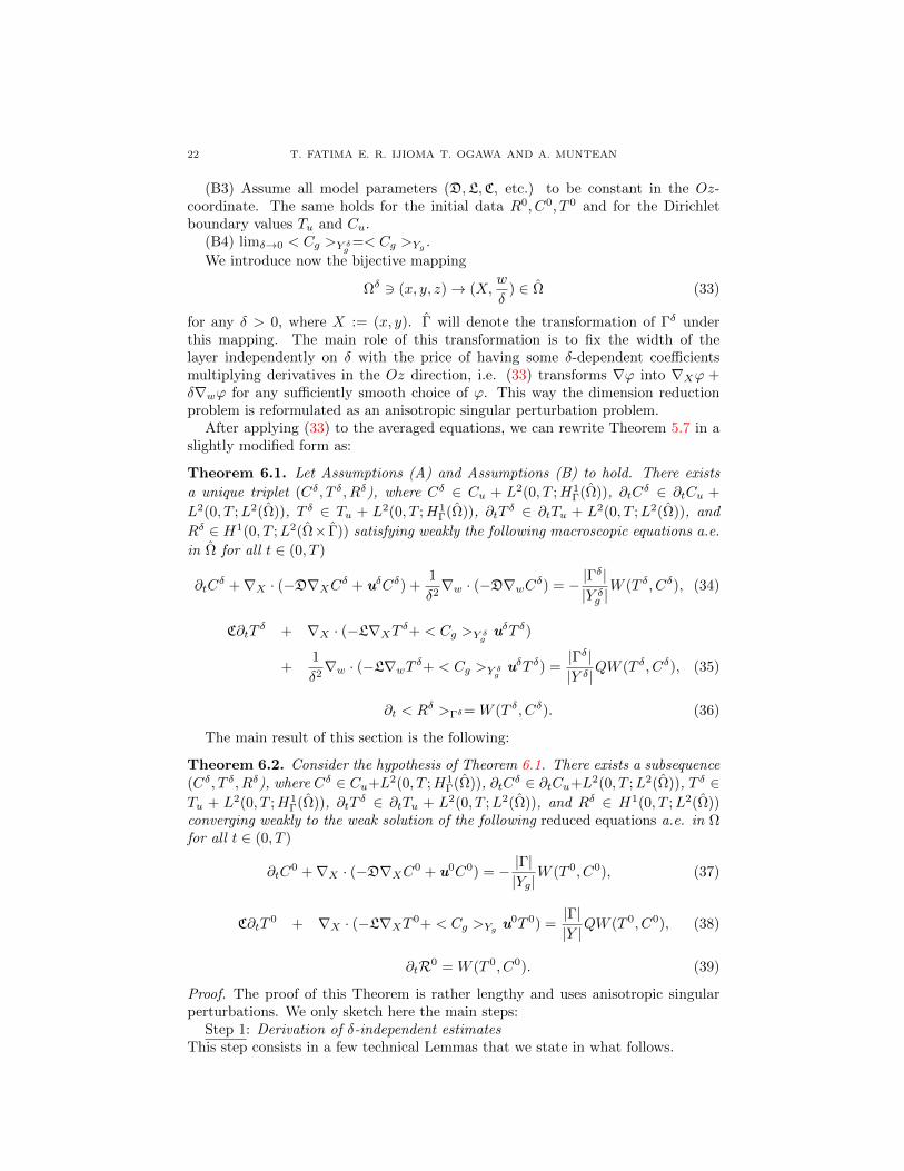
for any δ > 0, where X := (x, y). Γ will denote the transformation of Γδ underthis mapping. The main role of this transformation is to fix the width of thelayer independently on δ with the price of having some δ-dependent coefficientsmultiplying derivatives in the Oz direction, i.e. (33) transforms ∇ϕ into ∇Xϕ +δ∇wϕ for any sufficiently smooth choice of ϕ. This way the dimension reductionproblem is reformulated as an anisotropic singular perturbation problem.
After applying (33) to the averaged equations, we can rewrite Theorem 5.7 in aslightly modified form as:
Theorem 6.1. Let Assumptions (A) and Assumptions (B) to hold. There exists
a unique triplet (Cδ, T δ, Rδ), where Cδ ∈ Cu + L2(0, T ;H1Γ(Ω)), ∂tC
δ ∈ ∂tCu +
L2(0, T ;L2(Ω)), T δ ∈ Tu + L2(0, T ;H1Γ(Ω)), ∂tT
δ ∈ ∂tTu + L2(0, T ;L2(Ω)), and
Rδ ∈ H1(0, T ;L2(Ω× Γ)) satisfying weakly the following macroscopic equations a.e.
in Ω for all t ∈ (0, T )
∂tCδ +∇X · (−D∇XCδ + uδCδ) +
1
δ2∇w · (−D∇wCδ) = − |Γ
δ||Y δg |
W (T δ, Cδ), (34)
C∂tTδ + ∇X · (−L∇XT δ+ < Cg >Y δg uδT δ)
+1
δ2∇w · (−L∇wT δ+ < Cg >Y δg uδT δ) =
|Γδ||Y δ|
QW (T δ, Cδ), (35)
∂t < Rδ >Γδ= W (T δ, Cδ). (36)
The main result of this section is the following:
Theorem 6.2. Consider the hypothesis of Theorem 6.1. There exists a subsequence(Cδ, T δ, Rδ), where Cδ ∈ Cu+L2(0, T ;H1
Γ(Ω)), ∂tCδ ∈ ∂tCu+L2(0, T ;L2(Ω)), T δ ∈
Tu + L2(0, T ;H1Γ(Ω)), ∂tT
δ ∈ ∂tTu + L2(0, T ;L2(Ω)), and Rδ ∈ H1(0, T ;L2(Ω))converging weakly to the weak solution of the following reduced equations a.e. in Ωfor all t ∈ (0, T )
∂tC0 +∇X · (−D∇XC0 + u0C0) = − |Γ|
|Yg|W (T 0, C0), (37)
C∂tT0 + ∇X · (−L∇XT 0+ < Cg >Yg u0T 0) =
|Γ||Y |
QW (T 0, C0), (38)
∂tR0 = W (T 0, C0). (39)
Proof. The proof of this Theorem is rather lengthy and uses anisotropic singularperturbations. We only sketch here the main steps:
Step 1: Derivation of δ-independent estimatesThis step consists in a few technical Lemmas that we state in what follows.

FILTRATION COMBUSTION IN HETEROGENEOUS THIN LAYERS 23
Lemma 6.3. Assume Assumptions (B). Then there exist (C0, T 0,R0) and a sub-sequence still labeled with δ converging to zero such that
(i) Cδ C0, ∇XCδ ∇XC0 and ∂tCδ ∂tC in L2((0, T );L2(Ω).
(ii) T δ T 0, ∇XT δ ∇XT 0 and ∂tTδ ∂tT in L2((0, T );L2(Ω).
(iii) < Rδ > R0 in L2((0, T ), L2(Ω)), ∂t < Rδ >∗ ∂tR0 in L∞((0, T ), L∞(Ω)).
(iv) W (T δ, Cδ) W (T 0, C0) in L2((0, T ), L2(Ω)).
Proof. (i)-(iii)The proof of these estimates follows the same line of the proof ofLemma 4.2 and Lemma 4.6. We omit to show it here. (iv) Note that we actually have
the strong convergence Cδ → C0 in L2((0, T );L2(Ω) as well as f(T δ) f(T 0) in
L2((0, T );L2(Ω). This concludes thatW (T δ, Cδ) W (T 0, C0) in L2((0, T ), L2(Ω)).Compare Lemma 5.5 (d).
Lemma 6.4. Under the assumptions of Lemma 6.3, the following statements holdtrue:
(i) For any ϕ ∈ H1Γ(Ω), the functions t →
∫ΩCδϕdx and t →
∫ΩC0ϕdx belong
to H1(0, T ) and for the same subsequence we have∫Ω
Cδϕdx→∫
Ω
C0ϕdx in L2(0, T ) and in C([0, T ])
and ∫Ω
Cδϕdx
∫Ω
C0ϕdx in H1(0, T ).
(ii) For any φ ∈ H1Γ(Ω), the functions t→
∫ΩT δφdx and t→
∫ΩT 0φdx belong to
H1(0, T ) and for the same subsequence we have∫Ω
T δφdx→∫
Ω
T 0φdx in L2(0, T ) and in C([0, T ])
and ∫Ω
T δφdx
∫Ω
T 0φdx in H1(0, T ).
Proof. The proof follows the lines of Lemma 3.3 in [8].
Step 2: (Recovering the weak and strong formulations of problem (P00))This step is more delicate and its success strongly depends on the regularity con-straints from Assumptions (B). We skip here the proof and refer the reader to [8],where a scalar case has been treated in full details. To recover the ordinary differ-ential equation for R0, one proves first that the sequence (Rδ) is a Cauchy sequencein a suitable functions space. Section 5.1 from [15] provides the insight needed toshow this property.
Step 3: (Uniqueness of weak solutions to problem (P00))Since the system is semi-linear, the globally Lipschitz non-linearity of the productionterm by chemical reaction ensures the desired uniqueness of (weak) solutions.
Step 4: (Removing the w-dependency. Projection on Ω)Integrating the PDE system over the w-variable reduces the formulation of the
model posed on Ω to a formulation posed on the ”plate” Ω. Integrating over thereaction term does not commute with the nonlinearity. This requires a proof of a
corrector estimate of the type |∫ 1
0W(T δ, Cδ
)dw−W
(∫ 1
0T δdw,
∫ 1
0Cδdw
)| ≤ Cδ,
with an appropriate constant C independent of the choice of δ (see Lemma 4.5 in[38] for a related corrector estimate).
24 T. FATIMA E. R. IJIOMA T. OGAWA AND A. MUNTEAN
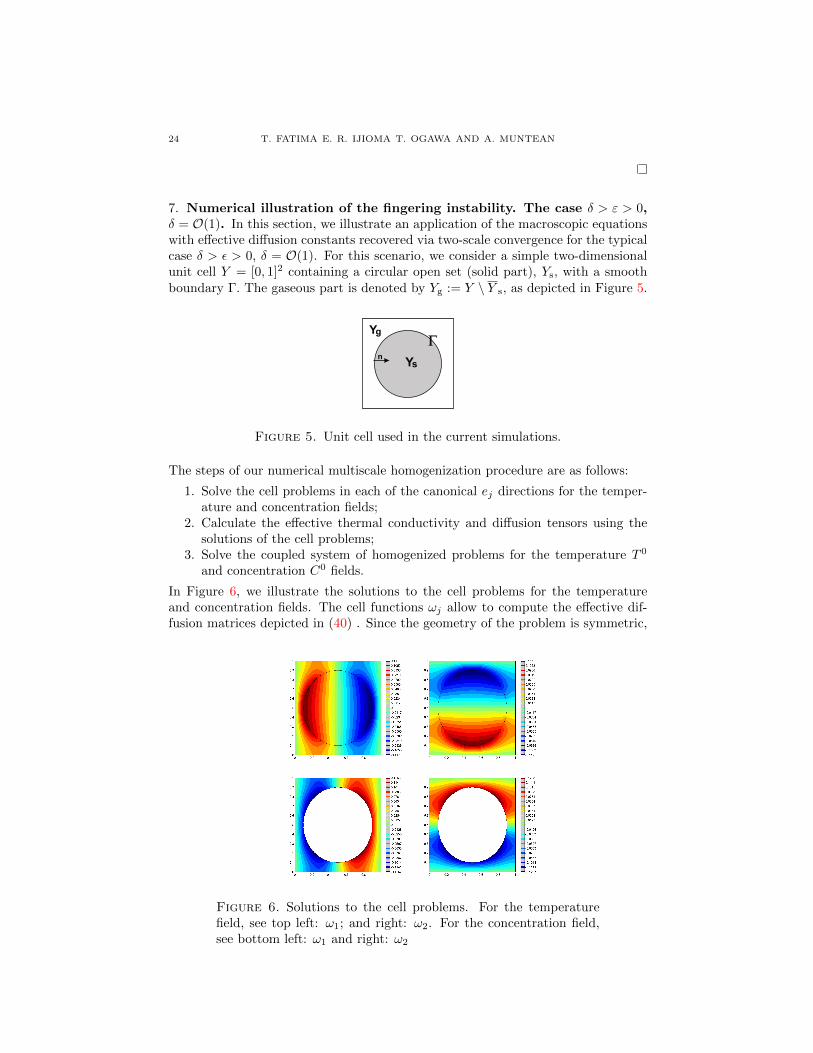
7. Numerical illustration of the fingering instability. The case δ > ε > 0,δ = O(1). In this section, we illustrate an application of the macroscopic equationswith effective diffusion constants recovered via two-scale convergence for the typicalcase δ > ε > 0, δ = O(1). For this scenario, we consider a simple two-dimensionalunit cell Y = [0, 1]2 containing a circular open set (solid part), Ys, with a smoothboundary Γ. The gaseous part is denoted by Yg := Y \ Y s, as depicted in Figure 5.
Yg
Ys
u
Figure 5. Unit cell used in the current simulations.
The steps of our numerical multiscale homogenization procedure are as follows:
1. Solve the cell problems in each of the canonical ej directions for the temper-ature and concentration fields;
2. Calculate the effective thermal conductivity and diffusion tensors using thesolutions of the cell problems;
3. Solve the coupled system of homogenized problems for the temperature T 0
and concentration C0 fields.
In Figure 6, we illustrate the solutions to the cell problems for the temperatureand concentration fields. The cell functions ωj allow to compute the effective dif-fusion matrices depicted in (40) . Since the geometry of the problem is symmetric,
Figure 6. Solutions to the cell problems. For the temperaturefield, see top left: ω1; and right: ω2. For the concentration field,see bottom left: ω1 and right: ω2

FILTRATION COMBUSTION IN HETEROGENEOUS THIN LAYERS 25
the effective thermal conductivity and diffusion constants are isotropic, and thecalculated values are given viz.
λeff =
(3.96 · 10−4 0.00
0.00 3.96 · 10−4
)Deff =
(0.080523 0.00
0.00 0.080523
). (40)
In the next step, the effective diffusion constants are used together with the upscaledequations in order to verify our homogenization process. The macroscopic system ofequations is used to verify the development of fingering instability of a thin poroussample subjected to a reverse smoldering combustion. The macroscopic behaviorof the captured flame structure is illustrated in Figure 7, where R0 is the smolderpattern on the surface of the sample. T 0 is the macroscopic temperature field, C0
the concentration and W is the nonlinear heat released rate.
Figure 7. Macroscopic profiles of the spatial structure of the flamefront: (a) Temperature T 0, (b) Reaction product R0, (c) Activeconcentration C0, (d) Heat released rate W (C0, T 0).
8. Discussion. We keep as further work the case δ = O(ε), when δ vanishes uni-formly (in space). Since the diagram of taking the limits ε → 0 and δ → 0 seemsto be commutative, we expect that the concept of thin heterogeneous convergencecf. [29] can be applied to (Pδε) in a rather straightforward way. The derivation ofcorrector estimates in terms of O(ε, δ) is open; this fact makes unavailable rigorous

26 T. FATIMA E. R. IJIOMA T. OGAWA AND A. MUNTEAN
MsFEM approximations for this multiscale problem. Particularly critical is how toproceed in the fast convection case uε = O
(1εα
)and/or in the fast reaction case
A = O(
1εβ
), with α > 0, β > 0 (or in suitable combinations of both).
(x) (x)
Figure 8. Heterogeneous thin layer of height of order of O(δ(x)):Microscopic view (left) and macroscopic view (right).
For a non-uniform shrinking of the layer (see Figure 8 for an illustration of thecase δ(x) → 0), we expect that a convergence in measures is needed to describehow the ”mass” and the ”energy” distribute on the flat supporting surface as thevolume of the layer vanishes; see [34] for a related context. Both cases δ(x) = O(1)and δ(x) = O(ε) are for the moment open.
Acknowledgments. This work is jointly supported by the Meiji University GlobalCenter of Excellence (GCOE) program ”Formation and Development of Mathemati-cal Sciences Based on Modeling and Analysis” and the Japanese Government (Mon-bukagakusho:MEXT). AM thanks the Department of Mathematics of the Universityof Meiji, Tokyo, Japan for their kind hospitality, which facilitated the completionof this paper. Partial support from the EU ITN FIRST is also acknowledged. Wethank I. S. Pop for showing us Ref. [38].
REFERENCES
[1] I. Aganovic, J. Tambaca, and Z. Tutek. A note on reduction of dimension for linear elliptic
equations. Glasnik Matematicki, 41(61):77–88, 2006.
[2] G. Allaire. Homogenization and two-scale convergence. SIAM J. Math. Anal., 23(6):1482–1518, 1992.
[3] G. Allaire and Z. Habibi. Homogenization of a conductive, convective, and radiative heat
transfer problem in a heterogeneous domain. SIAM J. Math. Anal., 45(3):1136–1178, 2013.[4] B. Amaziane, L. Pankratov, and V. Pytula. Homogenization of one phase flow in a highly
heterogeneous porous medium including a thin layer. Asymptotic Analysis, 70:51–86, 2010.
[5] M. Benes and J. Zeman. Some properties of strong solutions to nonlinear heat and moisturetransport in multi-layer porous structures. Nonlinear Anal. RWA, 13:1562–1580, 2011.
[6] G. Chechkin, A. L. Piatnitski, and A. S. Shamaev. Homogenization Methods and Applications,volume 234 of Translations of Mathematical Monographs. AMS, Providence, Rhode IslandUSA, 2007.
[7] M. Chipot. ` goes to infinity. Birkhauser, Basel, 2002.[8] M. Chipot and S. Guesmia. On some anisotropic, nonlocal, parabolic singular perturbations
problems. Applicable Analysis, 90(1):1775–1789, 2011.[9] D. Cioranescu and P. Donato. An Introduction to Homogenization. Oxford University Press,
New York, 1999.[10] D. Cioranescu and J. S. J. Paulin. Homogenization in open sets with holes. J. Math. Anal.
Appl., 71:590–607, 1979.[11] D. Cioranescu and A. Oud Hammouda. Homogenization of elliptic problems in perforated
domains with mixed boundary conditions. Rev. Roumaine Math. Pures Appl., 53(5-6):389–
406, 1998.[12] D. Cioranescu and J. Saint Jean Paulin. Homogenization of Reticulated Structures. Springer
Verlag, Berlin, 1999.
FILTRATION COMBUSTION IN HETEROGENEOUS THIN LAYERS 27
[13] P. Constantin, A. Kiselev, A. Oberman, and L. Ryzhik. Bulk burning rate in passive-reactivediffusion. Arch. Rational Mec. Anal., 154:53–91, 2000.
[14] A. Fasano, M. Mimura, and M. Primicerio. Modelling a slow smoldering combustion process.
Math. Methods Appl. Sci., 33:1–11, 2009.[15] T. Fatima and A. Muntean. Sulfate attack in sewer pipes: Derivation of a concrete corrosion
model via two-scale convergence. Nonlinear Analysis: Real World Applications, 15(1):326–344, 2014.
[16] B. Gustafsson and J. Mossino. Non-periodic explicit homogenization and reduction of dimen-
sion: the linear case. IMA J. Appl. Math., 68:269–298, 2003.[17] Z. Habibi. Homogeneisation et convergence a deux echelles lors d echanges thermiques sta-
tionnaires et transitoires. Application aux coeurs des reacteurs nucleaires a caloporteur gaz.
PhD thesis, Ecole Polytechnique, Paris, 2011.
[18] U. Hornung. Homogenization and Porous Media. Springer-Verlag New York, 1997.
[19] U. Hornung and W. Jager. Diffusion, convection, absorption, and reaction of chemicals inporous media. J. Diff. Eqs., 92:199–225, 1991.
[20] E. R. Ijioma. Homogenization approach to filtration combustion of reactive porous materials:
Modeling, simulation and analysis. PhD thesis, Meiji University, Tokyo, Japan, 2014.[21] E. R. Ijioma, A. Muntean, and T. Ogawa. Pattern formation in reverse smouldering combus-
tion: a homogenisation approach. Combustion Theory and Modelling, 17(2):185–223, 2013.
[22] K. Ikeda and M. Mimura. Mathematical treatment of a model for smoldering combustion.Hiroshima Math. J., 38:349–361, 2008.
[23] K. Kumar, M. Neuss-Radu, and I. S. Pop. Homogenization of a pore scale model for precipi-
tation and dissolution in porous media. CASA Report, (13-23), 2013.[24] J. L. Lions. Quelques methodes de resolution des problemes aux limites nonlineaires. Dunod,
Paris, 1969.
[25] Z. Lu and Y. Dong. Fingering instability in forward smolder combustion. Combustion Theoryand Modelling, 15(6):795–815, 2011.
[26] S. Monsurro. Homogenization of a two-component composite with interfacial thermal barrier.Adv. Math. Sci. Appl., 13(1):43–63, 2003.
[27] S. Neukamm and I. Velcic. Derivation of a homogenized von-Karman plate theory from 3D
nonlinear elasticity. Mathematical Models and Methods in Applied Sciences, 23(14):2701–2748, 2013.
[28] M. Neuss-Radu. Some extensions of two-scale convergence. C. R. Acad. Sci. Paris. Mathe-
matique, 323:899–904, 1996.[29] M. Neuss-Radu and W. Jager. Effective transmission conditions for reaction-diffusion pro-
cesses in domains separated by an interface. SIAM J. Math. Anal., 39(3):687–720, 2007.
[30] G. Nguestseng. A general convergence result for a functional related to the theory of homog-enization. SIAM J. Math. Anal, 20:608–623, 1989.
[31] A.A.M Oliveira and M. Kaviany. Nonequilibrium in the transport of heat and reactants in
combustion in porous media. Progress in Energy and Combustion Science, 27:523–545, 2001.[32] S.L. Olson, H.R. Baum, and T. Kashiwagi. Finger-like smoldering over thin cellulose sheets in
microgravity. Twenty-Seventh Symposium (International) on Combustion, pages 2525–2533,1998.
[33] I. Ozdemir, W. A. M. Brekelmans, and M. G. D. Geers. Computational homogenization forheat conduction in heterogeneous solids. International Journal for Numerical Methods inEngineering, 73(2):185–204, 2008.
[34] I. A. Bourgeat G. A. Chechkin A. L. Piatnitski. Singular double porosity model. Applicable
Analysis, 82(2):103–116, 2003.[35] M. Sahraoui and M. Kaviany. Direct simulation vs volume-averaged treatment of adiabatic
premixed flame in a porous medium. Int. J. Heat Mass Transf., 37:2817–2834, 1994.[36] H. F. W. Taylor. Cement Chemistry. London: Academic Press, 1990.[37] C. van Duijn, A. Mikelic, I. S. Pop, and C. Rosier. Mathematics in chemical kinetics and
engineering, chapter on Effective dispersion equations for reactive flows with dominant Peclet
and Damkohler numbers. Academic Press, pages 1–45, 2008.[38] C. J. van Duijn and I. S. Pop. Crystal dissolution and precipitation in porous media: Pore
scale analysis. J. Reine Angew. Math, 577:171–211, 2004.[39] J.-P. Vassal, L. Orgeas, D. Favier, and J.-L. Auriault. Upscaling the diffusion equations in
particulate media made of highly conductive particles. I. Theoretical aspects. Physical Review
E, 77(011302):785–795, 2008.
28 T. FATIMA E. R. IJIOMA T. OGAWA AND A. MUNTEAN
[40] F. Yuan and Z. Lu. Structure and stability of non-adiabatic reverse smolder waves. AppliedMathematics and Mechanics, pages 1–12, 2013.
[41] O. Zik, Z. Olami, and E. Moses. Fingering instability in combustion. Phys. Rev. Lett., 81:3868–
3871, 1998.
E-mail address: [email protected]
E-mail address: [email protected]
E-mail address: [email protected]
E-mail address: [email protected]

PREVIOUS PUBLICATIONS IN THIS SERIES:
Number Author(s) Title Month
13-33 13-34 13-35 14-01 14-02
Q. Hou A.C.H. Kruisbrink F.R. Pearce A.S. Tijsseling T. Yue Q. Hou A.S. Tijsseling Z. Bozkus Q. Hou A.S. Tijsseling J. Laanearu I. Annus T. Koppel A. Bergant S. Vučkovič A. Anderson J.M.C. van ’t Westende A. Di Bucchianico E.J.W. ter Maten R. Pulch R. Janssen J. Niehof M. Hanssen S. Kapora T. Fatima E.R. Ijioma T. Ogawa A. Muntean
Smoothed particle hydrodynamics simulations of flow separation at bends Dynamic force on an elbow caused by a traveling liquid slug Experimental investigation on rapid filling of a large-scale pipeline Robust and efficient uncertainty quantification and validation of RFIC isolation Homogenization and dimension reduction of filtration combustion in heterogeneous thin layers
Dec. ‘13 Dec. ‘13 Dec. ‘13 Jan. ‘14 Febr. ‘14
Ontwerp: de Tantes,
Tobias Baanders, CWI