Homoclinic bifurcations and dimension of attractors for...
36
INSTITUTE OF PHYSICS PuBusIDNG NoNLINEARITY Nonlinearity 16 (2003) 2163-2198 PII: S09S1-771S(03)S8683-2 Homoclinic bifurcations and dimension of attractors for damped nonlinear hyperbolic equations Dmitry Turaev 1 and Sergey Zelik 2 1 WIAS, Mohrenstr. 39, D-10117 Berlin, Germany 2 Universite de Poitiers, Laboratoire d' Applications des MatMmatiques-SP2MI, Boulevard Marie et Pierre Curie-T616port 2, 86%2 Chasseneuil Futuroscope Cedex, France E-mail: [email protected]@mathlabo.univ-poitiers.fr Received 20 January 2003, in final form 4 July 2003 Published 15 September 2003 Online at stacks.iop.orgINonlI6l2163 Recommended by P Constantin Abstract A new method of obtaining lower bounds for the attractor's dimension is suggested which involves analysis of homo clinic bifurcations. The method is applied for obtaining sharp estimates of the attractor's dimension for a class of abstract damped wave equations which are beyond the reach of the classical methods. Mathematics Subject Classification: 35B41, 37G20, 35B45, 37045 o. Introduction It is well-known that the long-time behaviour of solutions of partial differential equations arising in mathematical physics can, in many cases, be described in terms of global attractors of the associated semigroups (see [1-4] and references therein). Moreover, it is also known that for a large class of equations of mathematical physics, including reaction-diffusion equations, Ginzburg-Landau equations, two-dimensional Navier-Stokes system, damped wave equations, etc, the corresponding attractor has finite Hausdorff and fractal dimensions. Thus, although the phase space for such problems is infinite-dimensional, the dynamics on the attractor happens to be finite-dimensional, hence it can possibly be understood by methods of the qualitative theory of ordinary differential equations. One of the crucial questions here is, of course, obtaining more or less realistic estimates for the dimension of the attractor. The best known upper estimates here are usually obtained based on the Kaplan-Yorke concept of Lyapunov dimension dimL(A) of the attractor A (see [5]), and on the following estimate: (0.1) 0951-7715/03/062163+36$30.00 II) 2003 lOP Publishing Ltd and LMS Publishing Ltd Printed in the UK 2163
Transcript of Homoclinic bifurcations and dimension of attractors for...
INSTITUTE OF PHYSICS PuBusIDNG NoNLINEARITY
Nonlinearity 16 (2003) 2163-2198 PII: S09S1-771S(03)S8683-2
Homoclinic bifurcations and dimension of attractors for damped nonlinear hyperbolic equations
Dmitry Turaev1 and Sergey Zelik2
1 WIAS, Mohrenstr. 39, D-10117 Berlin, Germany 2 Universite de Poitiers, Laboratoire d' Applications des MatMmatiques-SP2MI, Boulevard Marie et Pierre Curie-T616port 2, 86%2 Chasseneuil Futuroscope Cedex, France
E-mail: [email protected]@mathlabo.univ-poitiers.fr
Received 20 January 2003, in final form 4 July 2003 Published 15 September 2003 Online at stacks.iop.orgINonlI6l2163
Recommended by P Constantin
Abstract A new method of obtaining lower bounds for the attractor's dimension is suggested which involves analysis of homo clinic bifurcations. The method is applied for obtaining sharp estimates of the attractor's dimension for a class of abstract damped wave equations which are beyond the reach of the classical methods.
Mathematics Subject Classification: 35B41, 37G20, 35B45, 37045
o. Introduction
It is well-known that the long-time behaviour of solutions of partial differential equations arising in mathematical physics can, in many cases, be described in terms of global attractors of the associated semigroups (see [1-4] and references therein). Moreover, it is also known that for a large class of equations of mathematical physics, including reaction-diffusion equations, Ginzburg-Landau equations, two-dimensional Navier-Stokes system, damped wave equations, etc, the corresponding attractor has finite Hausdorff and fractal dimensions. Thus, although the phase space for such problems is infinite-dimensional, the dynamics on the attractor happens to be finite-dimensional, hence it can possibly be understood by methods of the qualitative theory of ordinary differential equations. One of the crucial questions here is, of course, obtaining more or less realistic estimates for the dimension of the attractor.
The best known upper estimates here are usually obtained based on the Kaplan-Yorke concept of Lyapunov dimension dimL(A) of the attractor A (see [5]), and on the following estimate:
(0.1)
0951-7715/03/062163+36$30.00 II) 2003 lOP Publishing Ltd and LMS Publishing Ltd Printed in the UK 2163
2164 D Tumev and S Zelik
where dimH and dimp denote the Hausdorff and the fractal dimension, respectively (see [7,6,3,8--10]). The main point here is that the Lyapunov dimension, by its definition, can be explicitly estimated using sufficiently simple volume-contraction arguments (see [3], chapter 5, for details).
Lower bounds for the attractor's dimension are usually based on the observation that the unstable manifold of any equilibrium of the system is always contained in the global attractor A. Consequently, the following estimate is valid:
dimF(A) :;. dimH(A) :;. maxN+(uo), (0.2) lIoe1i
where n is the set of equilibria of the system, and N+(uo) is the instability index of the equilibrium Uo (see, e.g., [1,2]).
We note that this method of obtaining the lower bounds for the attractor's dimension is perfect for the class of gradient systems (or, which is slightly more general, for systems possessing a global Lyapunov function). Indeed, the dynamics in the gradient case is, in a sense, trivial and the dimension of the attractor is determined by the instability indices of the equilibria only, no matter what the Lyapunov dimension of the attractor and what the volume-contraction properties. Namely, in this case we have the equality in the second part of (0.2):
(0.3)
(see, e.g., [I, II]). There exists, however, a number of important equations of mathematical physics (such as
two.{\imensional Navier-Stokes system, Ginzburg-Landau equations, non-gradient systems of damped wave equations), for which the given methods of estimating the attractor's dimension from above and below yield different asymptotics for the dimension in terms of physical parameters of the system (see [3], chapter 6, [4] and references therein). Which asymptotics is then correct is a long-standing open problem in the theory of attractors. It is also worth noting that all systems mentioned above are far from being gradient and they usually demonstrate a very complicated (e.g. chaotic) dynamical behaviour.
In this paper, we present a new method of obtaining lower bounds for the attractor's dimension which exploits explicitly the recurrent (as opposed to gradient-like) nature of the system, and which is based on some general ideas from the theory of homo clinic bifurcations. Namely, we suggest estimating from below the attractor's dimension in terms of the maximum M (r, uo) of the dimension of the unstable manifold over the periodic orbits which can be born at a bifurcation of a homo clinic orbit r to an equilibrium Uo:
(0.4)
To be more precise, one should consider a family of systems which depends on some set of parameters /L; then the global attractor is a function of /L as well, and (0.4) shonld be interpreted as
where the bifurcational moment /L = /Lo corresponds to the existence of the homoclinic loop r. Of course, one may use various homolheteroclinic cycles with the same purposes---we take a homoclinic loop as the simplest possible construction.
The power of the homoclinic bifurcation theory is that it allows one to obtain a lot of knowledge about the behaviour of a dynamical system, based only on a very limited amount of information about it. The most prominent example is the Shilnikov homo clinic loop theorem: if a system has a homoclinic loop to an equilibrium whose nearest to the imaginary axis
Homoclinic loops and dimension of attractors 2165
characteristic roots are complex, then the behaviour of orbits is chaotic, with a very detailed description of this behaviour available [12, 13]. The famous Lorenz attractor, as well as its higher-dimensional generalization-a wild spiral attractor-also appear as a result of a bifurcation of certain homoclinic loops (see [14-16]).
As found in [17], the common feature of various homo clinic bifurcations is that the behaviour near a homolheteroclinic cycle is very much related to the Lyapunov dimension of equilibria and periodic orbits involved. In particular, for many classes of homoclinic loops the dimension M (r, uo) essentially coincides with the Lyapunov dimension of the corresponding equilibrium Uo:
M(r, uo) ~ dimduo), (0.5)
no matter how small the dimension N+(uo) of the unstable manifold of Uo is. Thus, under this approach, both upper and lower bounds for the attractor's dimension are given in terms of Lyapunov dimension. That is why we expect this method to be effective in order to obtain sharp bounds for the dimension. Of course, the existence of a homoclinic orbit and the possibility of perturbing it in the desired way within the class of systems under consideration is crucial for this method. However, the homoclinic phenomena are so typical for dynamical systems with non-trivial behaviour, that it would be natural to expect that in a wide class of equations of mathematical physics which demonstrate chaotic behaviour appropriate homoclinic bifurcations can indeed be detected (see, e.g., [18--21] where the existence of homoclinic loops was proven for the noulinear Schrodinger and sine-Gordon equations).
We illustrate our method by a model example of an abstract damped wave equation
0t'U + YOtU + Au = F(u, Otu) (0.6)
in a Hilbert space H. We assume that A : D(A) --> H is a positive self-adjoint operator in H with compact inverse, whose eigenvalues satisfy the estimate
(0.7)
for some positive Ch C, and /c. Natural examples for A are provided by elliptic differential operators in a bounded domain, with H = L'. The quantity Y > 0 in (0.6) is a dissipation (or damping) parameter which is assumed to be small. To avoid technicalities, we have also assumed that the noulinear operator F = F(u, Otu) belongs to some class S of very regular ('smoothing') operators which will be specified in section 2. Note that this class does not include superposition operators: we do not intend to apply our method to any specific equation in this paper, we ouly want to exemplify the basic ideas, so we restrict our consideration to this sufficiently simple setting.
We prove that under the above assumptions, equation (0.6) possesses a global attractor A in the corresponding energetic space E, and the Lyapunov dimension of the attractor satisfies
C;y-I .;;; dimdA) .;;; C2y-1 (0.8)
for some positive constants C;., which are independent of y. Consequently, due to (0.1), we have
(0.9)
On the other hand, when the noulinearity belongs to our class S of very regular operators, we show that for every B > 0 there exists a positive constant C, such that the instability index of any equilibrium state is less than C,y-'. Thus, using the classical methods of estimating the dimension of the attractor A (which are based on (0.1) and (0.2)), we will necessarily have a huge gap between the asymptotics for upper and lower bounds of the attractor's dimension.
2166 D Tumev and S Zelik
Nevertheless, using our 'homoclinic' method, we construct nonlinearities F belonging to the same class S, for which we have
<limF(A) ;;. <limH(A) ;;. C3y-1 (0.10)
for some positive constant C3• Thus, at least in the case of damped hyperbolic equations with smoothing nonlinearities, the correct asymptotics for the <limension of the attractor is given by the corresponding asymptotics of the Lyapunov <limension, and the estimate (0.2) is not very relevant.
Note also that A is the so~alled maximal attractor, so it could be possible, in principle, that the dimension of A can be decreased drastically by removing from A non-recurrent orbits (as in gradient-like systems where such an operation reduces A to a zero-dimensional set, typically). We show, however, that nonlinearities F E S exist for which equation (0.6) has a mininIal set whose <limension satisfies (0.10); therefore, the Lyapunov <limension (up to a constant factor) measures the complexity of the dynantics of damped hyperbolic equations correctly.
The examples which we are talking about are obtained as small perturbations of a decoupled system of second order ODEs (see (4.6)) which is an infinite collection of damped linear oscillators plus a single one degree of freedom Hamiltonian system describing a particle in a double-well potential on a straight line. Note that none of the modes here shows chaotic behaviour and, moreover, all of them but one are damped. We show, however, that for any fixed value of the damping parameter y > 0, a (non-local) interaction of an arbitrarily small strength can be arranged between these modes such that extremely complicated behaviour is ignited, involving a huge (~I/y) number of modes (see remark 4.3). Note that we nowhere use the linear character of the oscillatory modes and our construction works for a chain of nonlinear damped oscillators as well. Therefore, our results should be applicable to perturbations of other integrable equations, such as the nonlinear Schrodinger equation, etc.
This paper is organized as follows. The existence of the global attractor for problem (0.6) is verified in section I. The upper bounds for fractal and Lyapunov dimension of this attractor are obtained in section 2. The quantity M (r, uo) is computed for a special class of homo clinic loops in section 3. Finally, in section 4, we show that such homoclinic orbits really appear in equations (0.6) with the nonlinearities belonging to the class S, then based on (0.4) we derive sharp lower bounds for the attractor's <limension.
1. Abstract nonlinear hyperbolic equation and its attractor
In this section, we study the following abstract nonlinear hyperbolic equation in a Hilbert spaceH:
at2u + yatu + Au = F(u, atu),
(1.1) ull==O = Uo, Otult=o = u~,
where u = u(t) is an unknown H-valued function, A : D(A) --> H is a given positive selfadjoint operator in H with compact inverse, y > 0 is a given positive number which is assumed to be small and F is a given nonlinear operator.
As usual (see, e.g., [22] and [3], chapter 4), we define a scale H' of Hilbert spaces associated with H via
(1.2)
(here and below (', .) denotes the inner product in H) and consider equation (1.1) as an evolution equation with respect to Ht) = [u(t), atu(t)] in the corresponding energetic phase spaces
E' := HHI x H', Ht) := [u(t), atu(t)] E E' (1.3)
Homoclinic loops and dimension of attractors 2167
(in fact, we will consider only the case where the initial dala [UO, u~] belong either to the space E:= EO, or to EI).
We assume that the nonlinear term F belongs to the space
F E Cl (E, H) (1.4)
of smooth and globally bounded operators. It is also assumed that the partial derivatives F~ and F~. satisfy the following conditions:
1. (F~(u,v)O,O) '" ~IIOIl~+CyIlOIl~_ ..
2. I(F~(u, v)w, 0)1 '" ~(lIwll~1 + 1I01l~) + Cy(lIwll~ + 1I01l~_1)' (1.5)
where [u, v], [w, 0] E E are arbitrary, y > 0 is the sarne as in equation (1.1), and the constant Cy is independent of [u, v] and [w, 0]. These inequalities mean simply that the nonlinear dependence on OtU is subordinate to the linear term yOtu.
The following theorem shows that under the above assumptions equation (1.1) generates a dissipative semigroup in the energetic space E.
Theorem 1.1. Let the assumptions (1.4) and (1.5) hold. Then, for every HO) := [u(O), Otu(O)] E E, equation (1.1) has a unique global solution ~(t) E C([O, 00), E) and the following estimate is valid:
IIW) II~ '" CII~(O) lI~e-Y' + Clo (1.6)
where the constants C and CI depend only on F, A and y. Consequently, equation (1.1) generates a semigroup
S,:E-->E, by S,~(O) := Ht). (1.7)
Moreover, this semigroup is globally Lipschitz continuous with respect to the initial data [u(O), o,u(O)] E E, i.e.
1I~I(t) - ~2(t)lI~ '" CeK'II~I(O) - ~2(0)1I~, (1.8)
where K and C depend only on A, y and F (and they are independent of the solutions u I (t) and U2(t) of problem (1.1».
If ~(O) EEl, then the corresponding solution ~(t) belongs to EI for every t ;;. 0 and satisfies the following estimate:
1I~(t)II~1 '" C2I1HO)II~le-Y'/8 + C3 (1.9)
for some positive constants C2 and C3 which depend only on A, F and y.
The proof of this theorem is quite Slandard, so we move it to appendix A. Let us now verify that the semigroup S, : E --> E possesses a global compact attractor
in the phase space E. Recall that the set AcE is called a global attractor for the semigroup S, : E --> E if the following conditions are satisfied:
1. A is compact in E; 2. A is strictly invariant with respect to S" i.e. S,E = E; 3. A attracts bounded subsets of East --> 00, i.e. for every bounded BeE and every
neighbourhood O(A) in E, there exists a number T = T(IIBIIE, 0) such that
StB C A, for t ;;. T (1.10)
(see, e.g., [1,3], chapter I, for details).
2168 D Tumev and S Zelik
Theorem 1.2. Let the assumptions of theorem 1.1 hold. Then semigroup (1. 7) associated with the nonlinear hyperbolic problem (1.1) possesses a global attraetor A. which is bounded in E '. This attractor is generated by all complete bounded solutions of (1.1):
A = (~(O), ~(t) := [u(t), 8,u(t)l, t E lRsolves (1.1) and IIW)IIE:;;; C., t E lR}.
Proof. According to the abstract attractor's existence theorem (see, e.g., [1]) the theorem will be proven if we verify the following conditions on the semigroup S,:
1. S, : E -+ E is continuous with respect to HO) for every fixed t ;;. O. 2. The semigroup S, possesses a compact attracting (in the sense of (1.10» set K cc E.
Let us verify these conditions. Indeed, the continuity of S, is given by theorem 1.1. So, we are left to verify the second condition. Th this end, we split the solution u(t) of (1.1) as follows: u(/) := v(/) + w(/), where v(/) is a solution of the following problem:
8,2v + (y + bA-1)8,v + Av + Mv - F(v, 8,v) = MU(/) + bA-18,u(t),
[v, 8,vll,:oO = O. (1.11)
Here M » 1 and b » 1 are sufficiently large positive constants which will be specified below. Consequently, the remainder function w(t) satisfies the equation
where
8,2W + (y + bA -1)8,w + Aw + Mw = 1'(I)W + 12(/)8,w,
[w, 8,wll,~o = HO),
1'(1) := 10' F~(su(l) + (1 - s)v(t), s8,u(t) + (1 - s)8,v(t» ds,
12(1) := 10' F~,.(SU(/) + (1 - s)v(/), s8,u(/) + (1 - s)8,v(/» ds.
(1.12)
(1.13)
We will prove that IIw(/) liE tends uniformly (with respect to small variations in initial conditions) to zero, and V(I) enters some fixed ball in E' as time grows. This ball is compact in E, so it can be taken as a desired attracting set K.
Lemma 1.1. Let the assumptions of theorem 1.1 hold. Then, there exist large positive constants M = M(y, F, A) and b = b(y, F, A) such that the solution w(t) of equation (1.12) satisfies the following estimate:
II [w(t), 8,w(t)1IlE:;;; C'e-·'II~(O)IIE (1.14)
for appropriate positive constants C' and a which are independent of u.
Proof. Taking the inner product in H of equation (1.12) with 8,w + [(y + bA -1)/21w(t), we derive the following relation:
8'[1I8,wll~ + IIwll~, + «y + bA-1)w, 8,w) + Mllwll~}
+~{1I8,wll~+ IIwll~l +Mllwll~+ «y +bA-1)w, 8,w))
= -bIl8,wll~_1 - bllwll~ - Mbllwll~_l - ~(1I8,wll~ + IIwll~, +Mllwll~) +2(1'(/)W, 8,w) + 2(12(/)8,w, 8,w) + (1'(l)w, (y + bA-1)w)
+(I'(t)8,w, (y+bA-1)w) - !«y+bA-' )8,w, (y+2bA-1)w) == hw(t).
(1.15)
Homoclinic loops and dimension of attractors
We recall that, by conditions (1.4) and fonnulae (1.13),
1I12 (tlllc(H.H) + IIl'(tlllc(Ht,H) .;; C,
where C is independent of u and I, and, by conditions (1.5),
(l2(I)o,W(I), o,w(I)) .;; ~ lIo,w II~ + Cy lIo,w(l) II~_"
2169
(1.16)
(1.17)
Estimating the right-hand side hw (I) of (1.15) by HOlder inequality and taking into account estimates (1.16) and (1.17), we obtain
hw(t) .;; (Cy - !b) lIotw(t)II~_, + (C~(l + b3) - M)lIwll~, (1.18)
where Cy and C~ are two positive constants which depend only on y, F and A, but are independent of b, M and u, Fixing now the constants M and b in such a way that
b = 2Cy , M ;;. C~(l + b3),
we obtain the inequality hw (I) .;; 0, Moreover, without loss of generality we assume that M is chosen in such a way that, in addition,
I«y + bA-')w, o,w)1 .;; !(lIo,wll~ + Mllwll~), Applying now Gronwall's inequality to (1.15), we obtain (1.14), Lemma 1.1 is proven,
Now we are ready to estimate the solution v(t) of equation (1.11), We rewrite this equation in the following equivalent fonn:
o;v + yBtv +Av - F(v, B,v) = MW(I) + bA -'B,w(l) := hM,.(t) ,
[v, B,v]I,,,", := 0,
This equation is a non-autonomous analogue of equation (I, I), Moreover, due to theorem 1.1 and lemma 1.1, the function hM,.(t) can be estimated as follows:
IIhM,.(I)II~t + IIBthM,.(t)II~';; CM,.(l + IIHO)II~e-·') (1.19)
for an appropriate constant CM,. which is independent of u, Consequently, using estimate (1.19) and the fact that v(O) = 0, B,v(O) = 0, arguing exactly as in the proof of theorem 1.1 (see appendix A), we obtain that the solution [v, B,v] of (1.11) belongs to the space COR., E') and satisfies the estimate
lI[v(t), B,v(I)]IIE' .;; C,(IIHO)IIEe-·' + 1) (1.20)
for some positive constants a and C, which depend on M and y, but are independent of u, Estimates (1.14) and (1.20) imply that the set
K := {~ E E', II~IIE' .;; 2C'}
is a compact (in E) attracting set for the semigroup S" Thus, all conditions of the abstract attractor's existence theorem are verified and theorem 1.2 is proven,
Remark 1.1. We recall that our conditions (1.4) and (1.5) imply that the operator F (along with its first derivatives F~ and F~,.) is globally bounded as II~ liE -+ 00, This simplifying assumption is enough for our purposes because in our examples of sharp upper and lower bounds for the attractor's dimension (see section 4) the nonlinearity F has a bounded support, In fact, more general nonlinearities (see, e,g, [22,23] and [3], chapter 4) can be treated in the same way,
Remark 1.2. We note that conditions (1.4) and (1.5) are, obviously, satisfied if
FE Ct(E-', H) (1.21)
for some positive exponent 8, In the following, we will often use this stronger condition (1.21) instead of conditions (1.4) and (1.5),
2170 D Tumev and S Zelik
2. Upper bounds for the attractor's dimension
In this section we show, using the standard volume·contraction technique, that the attractor A of (1.1) constructed in the previous section has finite Hausdorff and fractal dimensions, and we obtain some estimates for this dimension in terms of the dissipation parameter y. To this end, we need the following assumption: there is an exponent K > 0 and two positive constants C I and C2 such that
i EN, (2.1)
where 0 < Al .;;; A2 .;;; ... are the eigenvalues of the operator A.
Remark 2.1. We note that assumption (2.1) is always satisfied if A is an elliptic differential operator in a bounded domain rl c JR" with a sufficiently smooth boundary and H := L2(rl) (see, e.g., [24]). Moreover, in this case K := kj2n, where k is the order of A.
In order to fonnulate the abstract theorem for estimating the dimension of invariant sets, we need the following definition.
Definition 2.1. A map S : A --+ A, where A is a subset of a certain Banach space E is called uniformly quasi-differentiable on A iffor any ~ E E there is a linear operator S'(~) : E --+ E (the quasi-differential) such that
holds uniformly with respect to ~I' ~ E A. It is also assumed that
sup IIS'(~)II£(E.E) < 00 ~eA
and S' E C(A, .c(E, E)).
(2.2)
(2.3)
Theorem 2.1. Let S, be a semigroup in a certain Hilbert space E and let ACE be a compact strictly invariant set of this semigroup (S,A = A). Let us suppose also that the semigroup S, is uniformly quasi-differentiable on Afor some fixed t = T and the following inequality holds for some positive integer d:
"'d(A) := SUP"'d(S~(m < 1, ~eA
(2.4)
where "'d(L) := IIAdLIlAdE is the norm of the dth exterior power of the operator L in the Hilbert space AdE (see, e.g., [31, chapter 5). Then the fractal dimension of A is finite in E. Moreover,
dimH(A, E) .;;; dimp(A, E) .;;; d. (2.5)
For the proof of this theorem see [3], chapter 5, for the case of Hausdorff dimension and [8--10] for the fractal dimension.
Lemma 2.1. Let the assumptions of theorem 1.1 hold. Then, semigroup (1.7), associated with hyperbolic equation (1.1), is uniformly quasi-differentiable on the anractor A and its quasi-differential S; (HO)) at ~ (0) E A is defined via the following standard expression:
S;(~(O))~ := [v(t), B,v(t)], (2.6)
where ~ E E and vet) is the solution of the equation of variations
B,2V + yB,v + Av = F~(u(t), B,u(t))v(t) + F~.(u(t), B,u(t))B,v(t),
[v, B,v]I,~ = ~, [u(t), B,u(t)] := S,~(O). (2.7)
Homoclinic loops and dimension of attractors 2171
The assertion of the lemma is completely standard, so we move its proof into appendix A. Thus, according to theorem 2.1, for estinJating the dimension of Ait is sufficient to estinJate
the norms of d-external powers for solving operator of equation of variations associated with the hyperbolic problem (1.1). To this end, following [22], we introduce a new variable OCt) := atu+(y /2)u(t) and rewrite system (1.1) in the equivalent form in variables [u, 0] E E. We obtain
(
_ru+O ) at (~) = y 2 yZ y'
F (u, 0 - 2u) + 4u - Au - 20 (2.8)
Now, insteadofapplyingtheorem2.1 to the initial system in [u, atu] variables we will use it for the transformed system (2.8) (since these systems are linearly equivalent, they have equivalent attractors whose dimensions coincide).
The equation of variations for the transformed system, obviously, has the form
at~(t) = lL(u(t), atu(t))~(t), [u(t), atu(t)] := StHO), (2.9)
where
1L := (-A + ~Z + F~(~) - ~F~.(g) -~ + ~~.(gJ (2.10)
In order to estinJate the exterior powers of solving operator S~(HO)) : ~ --> ~(T) of linear problem (2.9), we use the following standard lemma (see [22] or [3], chapter 5).
Lemma 2.2. Let the assumptions of lemma 2.1 hold. Then
(2.11)
where Trd(L) means the d-dimensional trace of the operator L : E --> E in E, i.e.
Trd(L) := sup {t(Lr" , ~;)E : II~; liE = I, (~;, ~j)E = ° fori # i} . 1=1
Now we are in a position to estinJate the fractal dimension of the attractor A of hyperbolic equation (1.1). For simplicity, we assume that the nonlinearity F satisfies condition (1.21) and estinJate the corresponding dimension in terms of parameters y, K (introduced in (2.1)) and 8 (introduced in (1.21)). (In the general case of conditions (1.4) and (1.5), this dimension can be analogously estinJated in terms of y, K and the constant Cy defined in (1.5).)
Theorem 2.2. Let the assumptions of theorem 1.1 hold and let, in addition, the nonlinearity F satisfy (1.21). Then, the fractal dimension of the attractor A is finite in E and can be estimated, as y --> 0, as follows
jY-ZIKI,
dimF(A,E)"':; CN(y):= C y-Zln~, y-2,
where C is independent of y --> 0, 8 > ° and K > 0.
K8 < 1,
K8 = I,
K8 > I,
Proof. According to theorem 2.1 and lemma 2.2, it is sufficient to prove that
(2.12)
sUP~eA Trd{lL(g)} < 0, for some d ",:; CN(y). (2.13)
2172 D Tumev and S Zelik
In order to show this, we first estimate the quadratic form associated with the operator L, usiug the assumptions (1.21) and Schwartz iuequality:
y 2 y2 (IL~, ~)E = -211~.IIHI + (~., A~.) - (~., A~.)+ 4(~U' ~.)
+ ((F~ - ~Fa,u) ~u,~.) - ~II~.II~ + (F~.~., ~.) ,;; -~(II~ull~1 + IIwll~) + Cy-l(lI~ull~l-' + II~.II~-,):= (B~, ~), (2.14)
where ~ := [~., ~.] E E, the operator B is defined as
B.=r(-Id+4Cy-2A-./2 0 ) . 4 0 -Id+ 4Cy-2A-'/2
and the constant C is iudependent of y, a and ~. It follows now from (2.14) that for any dEN,
Trd{lL} ,;; Trd{B}. (2.15)
We now observe that the operator B is self-adjoiut, hence, by the classical miu-max priuciple (see, e.g., [3], chapter 5), its traces can be immediately expressed iu terms of its eigenvalues, namely,
(2.16)
where Ai are the eigenvalues of A. The estimate (2.13) is an immediate corollary of (2.15), (2.16) and of the assumption (2.1) on the asymptotics of Ai. Theorem 2.2 is proven.
The followiug theorem shows that the estimate (2.12) can be essentially improved if the additional regularity of the nonliuear term F is known.
Theorem 2.3. Let the assumptions of theorem 1.1 hold and let, in addition,
(2.17)
where s > - ~ is some regularity exponent. Then, the dimension of the corresponding attractor A can be estimated via
I«s + ~) < I,
I«s + ~) = I,
I«s + ~) > I,
where the constant C 1 depends on s and F, but is independent of y.
Proof. Indeed, due to condition (2.17), we have the followiug estimates:
I(F~(u, iJtu)~u, ~.)I ,;; 1!F~(u, iJtu)~ullH'.I"II~.IIH--I/' ,;; c(1I~u 1I~~I" + 1I~.II~_-I/')
and, analogously,
(2.18)
(F~u(u, 1J,u)~., ~.) ,;; l!Fa,.(u, iJtu)~.IIH'.I"II~.IIH-'-I" ,;; CII~.II~_-I'" where the constant C depends only on F. These estimates allow (2.14) to be improved iu the followiug way:
(IL~, ~)E ,;; (B,~, ~)E'
Homoclinic loops and dimension of attractors
where
Y (-Id + Cy-1 A -(>+1/2)/2 B '--,.- 4 0
2173
-Id + CY-~ A -(H1/2)/2)
for some constant C > 0 which is independent of y (the term (y /2)(F~.~., ~6) in (2.14) is of order y and does not require additional estimates).
Computing now the d-dimensional trace of the operator B, in terms of the eigenvalues Ai, using asymptotics (2.1) for them and arguing as in the end of theorem 2.1 we derive the improved estimate (2.18).
Corollary 2.1. Let the assumptions of theorem 1.1 hold and let, in addition, (2.17) be satisfied with the exponent s > 1/" - !. Then, the dimension of the attraetor A possesses the fol/owing upper bound:
asy ~ 0, (2.19)
where the constant C is independent of y.
Let us now introduce the class S of smoothing nonlinearities F.
Definition 2.2. A nonlinear operator F : E ~ H belongs to the class S = S(Ck,m) if, for every m E JR., this operator belongs to C""(E-m, Hm) and the following estimates valid, for every k E 1\1 U (OJ:
IlFlic/(E-',iI") .;; Ck,m
for appropriate constants Ck,m'
(2.20)
Corollary 2.2. Let the eigenvalues of the operator A satisfy condition (2.1) and let the nonlinearity F belong to the class S. Then, thefraetal dimension of the corresponding global attraetor A associated with equation (1.1) possesses the fol/owing upper estimate:
. 1 dimF(A,E)';; C-, (2.21)
Y where the constant C depends on constants C
"m (defined in (2.20)) and on constants C" C2
and" (defined in (2.1)), but are independent ofy.
Remark 2.2. In section 4, we will show that even in the case of extremely regularnonlinearities F E S, the dimension of the attractor A may indeed have the rate growth ~y-1 as y ~ o. So, estimate (2.21) is indeed sharp in the limit y ~ O.
3. Bifurcations of a homoclinic loop and Lyapunov dimension
In this section, we consider bifurcations of a certain type of homoclinic loops; the resnlts will be essentially used in the next section in order to obtain sharp lower bounds for the fractal dimension of the attractor A in the class S.
In contrast to the previous sections, we consider here finite-dimensional systems of ODEs, namely, systems of the following form:
y = Ay + IF(y) ,
where the nonlinearity IF(y) belongs to C""(R", JR") and satisfies
IF(O) = IF' (0) = O.
(3.1)
(3.2)
We assume that the matrix A E .c(JR", JR") has only one eigenvalue to the right of the imaginary axis. By scaling the time variable in (3.1) we can always make this eigenvalue equal to I.
2174 D Tumev and S Zelik
The rest of the spectrum consists ofm pairs of complex eigenvalues (-A,±WI. ... , -Am±w,.) and (n-2m-I) eigenvalues whose real parts are less than some -Am+, < -Am' Herem is some positive integer such that 2m+ I .;; n, and A = (A" . ", Am) E Rm andw = (WI. ... ,w,.) E Rm are given vectors satisfying the condition
Wk > 0, k = 1, ... , m. (3.3)
We assume that the matrix A can be brought to the following form by a linear transformation of coordinates:
I 0 0 0 0 R, 0 0
A'- ( -A, w, ) (3.4) R. := -Ak ' -w.
0 0 Rm 0 0 0 0 A
where the matrix A E C(Rn- 2m-', Rn- 2m-') satisfies the spectral assumption:
Recr(A) .;; -Am+, (3.5)
Such transformation can always be done when all w are different. We, however, prefer not to make this assumption. Instead, we simply assume that the matrix A is in the form (3.4).
Accordingly, denoting y = (z, (Ul. v,), ... , (um , vm ), w), system (3.1) is written in the following form:
z =Z+"',
Uk = -AtU1 + lVtV,t + ... .
ilk = -(UkUk - A.tVk + ... , k= 1, ... ,m, (3.6)
til = Aw +"',
where the dots in (3.6) stand for the nonlinearities, i.e. for the terms vanishing at the origin along with their first derivatives.
By construction, system (3.1) has a hyperbolic equilibrium at the origin 0 : y = O. Moreover, the unstable manifold WU(O) is one-dimensional here, and it is tangent to the z-axis at the origin. WU\ 0 consists of two orbits (the separatrices) which leave the origin at t = -00 in opposite directions. We assume that one of the separatrices which leaves 0 towards positive z (we denote this separatrix as r) returns to the origin as t --> +00, thus it forms a homo clinic loop.
The system under consideration has an (n - 2m - I) -{\imensional smooth invariant strungstable manifold W" which is tangent at 0 to the w-space and which consists of all orbits which tend to 0 faster than e-l.· t (see, e.g., [25], chapter 5). We assume that the homoclinic loop r belongs to W", i.e. it enters 0 being tangent to the w-space. Note that this is a bifutcation of codimension (2m + I), so we study here a problem which is, at large m, very degenerate from the point of view of the conventional bifutcation theory. However, the homoclinic loops of these type are quite typical for integrable equations with dissipation (see, e.g., system (4.6) in the next section).
Finally, we assume that
(3.7)
Remark 3.1. We note that inequalities (3.5) and (3.7) imply that the flow defined by (3.6) contracts (2m + 2)-dimensional volumes near 0 while (2m + I)-dimensional volumes are not
Homoclinic loops and dimension of attractors 2175
contracted. Thus, the Lyapunov dimension dimL(A) of sys10m (3.1) at the origin possesses the estimates (see, e.g., [3], chapter 5):
2m + I < dimL(An) < 2m + 2.
The main result of this section is the following theorem.
Theorem 3.1. Lelthe above assumptions hold. Letn := {iLl, ... , iL2mj be an arbitrary set of 2m non·zero complex numbers such that if iL belongs to the set 'R., then its complex·conjugate jibelongs to n as well. Then, by an arbitrarily small Coo ·perturbation of system (3.1), a periodic orbit with 2m multipliers equal to iLl, •.. , iL2m and with the rest of the multipliers inside the unit circle can be bomjrom the homoclinic loop, i.e. for an arbitrarily small neighbourhood V of the homoclinic loop r, for every 8 > 0 and every r E 1'1, there exists a Coo ·function lGe satisfying the inequality
IIIG, - (An + IF) IIc'(ll<.,R') .;; 8,
such thot the perturbed system jI = 1G,(y) possesses a periodic orbit of the type described above, which lies in V.
Proof. Let us first locally straighten invariant manifolds WU, W' and W" c W', i.e. we make
a coordina1o transfonnation in a small neighbourhood of the origin such that the sys10m takes, locally, the form
Z = z(1 + p(y)),
14, = -A,u, + w.v. + f>(y) . (u, v, w),
il. = -w.u. - A.v. + g.(y) . (u, v, w),
w = (A + q(y))w,
k= 1, ... ,m, (3.8)
where the functions f> (y), g. (y), p (y), q (y) vanish at the origin. In these coordina1os we have W~, = {(ut. Vk) = 0 (k = I, ... , m), W = OJ, W~, = {z = OJ, WI:!, = {z = 0, (u., Vk) = 0 (k = I, ... , m) j, so the invariant manifolds are straigh10ned indeed. When the sys10m is brought to this form, we can freely change the characieristic exponents (i.e. -A. ± iw. and the eigenvalues of A) by localized small perturbations, without destroying the homoc1inic loop. Indeed, we may arbitrarily add small localized perturbations to the coefficients At. w. and A in (3.8), and this will not move the local invariant manifolds W~" WI:"', Wt,',. Thus, by applying perturbations of this kind, we will still have a homoc1inic loop which enters 0 lying in Wl~' So, we may always assume that
(3.9)
Moreover, we may always achieve by an arbitrari1y small such perturbation that the set of characteristic exponents is non·resonant. After that is done, Sternberg's theorem [26] is applied which means that we can make a smooth coordina1o transfonnation which makes the system linear in a small neighbourhood of 0, i.e. the sys10m takes, locally, the form
Z =Z,
Uk = -AkUk + lVkVt,
Vk = -CUkUk - AkVk,
w=Aw.
k= 1, ... ,m,
In other words, after the above transfonnations, our equation reads
jI = A(w)y + IF(y) , y := (z. Ul. VI • ...• Un. Vn • W) E lin
(3.10)
(3.11)
2176 D Tumev and S Zelik
with the matrix A given by (3.4) (from now on, we fix J,. satisfying (3.7) and (3.9), but we will vary the values of "''' ... , ..... , therefore we indicate the dependence of A on '" explicitly). The smooth nonlinear function IF vanishes in some neighbourhood 0 of the origin
IF(y) == 0 for YEO. (3.12)
Thus, by construction, the intersection of the homoclinic loop r with 0 consists of two pieces. The first piece, corresponding to large negative times, coincides with the positive local z-axis, and the second piece, corresponding to large positive I, lies in the w-space.
The solution of (3.10) which starts in 0 at a point (ZO, u~, v~, ... , u~, v~, wO) is written as
z(t) = zOe',
u,(t) = e-A"(u2cos""t +vZsin""t),
v,(t) = e-A" (-u2 sin ""I + v2 cos ""t), wet) = eA'wO.
(3.13)
We take some small d > 0 and consider two cross-sections to the homoclinic loop: nOll' = {z = d} and nm = {lIwllA = d} where the metric IIwllA in the w-space IRn
-2m-, is
defined as follows:
IIwlI~:= 100
lIeA'wll2dl
and II . II is a standard nonn in IRn- 2m-'. Then, obviously,
:1 (lIw II~) = -211w 112 < 0
and, consequently, every non-zero solution w = w(l) of equation tV = Aw intersects transversely the ellipsoid II w II A = d at a unique point. Therefore, the Poincare section nm is, indeed, well defined. Let also Wo correspond to the intersection point of the homoclinic loop with nm, and let a E IRn- 2m- 2 be local coordinates on the ellipsoid IIw IIA = d near Wo, i.e. there is a smooth function W : IRn- 2m- 2 -+ IRn- 2m-, such that IIW(a) IIA == d, W(O) = Wo
and W' (0) = Id. We introduce the local coordinates for M E nm and M E nOll' as follows
M(Z, Ut, VI, ... , Um, Vm , a) := (d· Z, Ul, Vh ... , Urn, Vm , W(a»,
M(uh Vl, ... , Um, Um, to) := (d, ill, ih, ... , Um, Vm, w).
According to (3.13), the orbit of a point M E nm with Z > 0 reaches nOll' at the moment of time I = -In Z, and the intersection of the orbit with n°ut is the point
M := T~O'(M) :=
ZA,(U, cos""lnZ - v, sin""lnZ) ZA,(U, sin""lnZ + v, cos""lnZ)
ZA, (u, cos "'k In Z - Vk sin "'k In Z) ZA, (u. sin "'k In Z + Vk cos ",.In Z)
Z-AW(a)
which defines the local Poincare map T~o, : nm n {Z > O} -+ nOll'.
(3.14)
Analogously, the orbits starting on nOll' close to the origin follow the homo clinic loop, so they come to the cross-section nm in finite time. These orbits define a global Poincare map
Tit° : n°ut -+ nm which is a diffeomorphism (since it is defined by orbits of a smooth flow in a finite time and since the trajectories intersect nm transversely). Thus, the linear operator
._ d glo To.- dMTo (0) (3.15)
Homoclinic loops and dimension of attractors 2177
is invertible and, due to our choice of coordinates in ITm and ITout ,
Tt(O) =0. (3.16)
Moreover, without loss of generality we assume that To E C(Rn-2m-2, IRn- 2m- 2) can be represented as follows:
To = Lo' Uo, (3.17)
where Uo and Lo are upper- and lower-triangular matrices, respectively:
L?, 0 Up, UP2 Up,
o o Lo = Uo = (3.18)
o o o
Indeed, decomposition (3.17) is well-known for generic invertible matrices To (and can be obtained, e.g., via a classical Gauss diagonalization procedure). If To is not generic, we can always put it in a general position by an arbitrarily small perturbation of the system, which is localized outside the d-neighbourhood of the origin and preserves the homoclinic loop (using the standard flow-box technique). Note that
for j = I, ... , n - 2m - 2, (3.19)
since To is invertible. We now consider an (m + n - I)-parameter family of small smooth perturbations of the
system (3.11), namely for every W E IRm which is sufficiently close to the original vector W := wo and for every sufficiently smalllJ E IRn-', we consider the following family of equations:
y = A(w)y +lFe,,,,(Y). (3.20)
We assnme that the function lFe,,,, is smooth with respect to all variables and satisfies the assnmptions
lFe.",(y) == 0 for YEO, and lFo,o(y) == IF(y) , (3.21)
wherelF(y) is defined in (3.11). Then, forsufficientlysmalllJ and (w-wo), the global Poincare map Tf.; : ITout -+ ITm is well defined and smooth. We assume that the perturbation (3.20) is such that this global Poincare map is written, in a small neighbourhood of the origin in IT°n!, as follows:
glo - glo -Te,,,,(M) = IJ + To (M), (3.22)
i.e. the ouly effect of the perturbation in the noulinearity IF is an additive term in the global map (see (3.16)). Obviously, such a family of perturbations exists (one can construct it by the flow-box technique). Since the global map is insensitive to changes in w we will further use the notation Tfo.
It is obvious that for every frequency vector w which is sufficiently close to WO and for every M E ITm n {Z > OJ which is sufficiently close to 0 (in our local coordinates on ITm) there exists a perturbation parameter IJ such that system (3.20) possesses a periodic orbit which intersects with ITm at the given point M. Indeed, note that, due to our construction, fixed points M with Z > 0 of the first-retorn map
Te,,,,(M) := Tf"(T!OC(M)), (3.23)
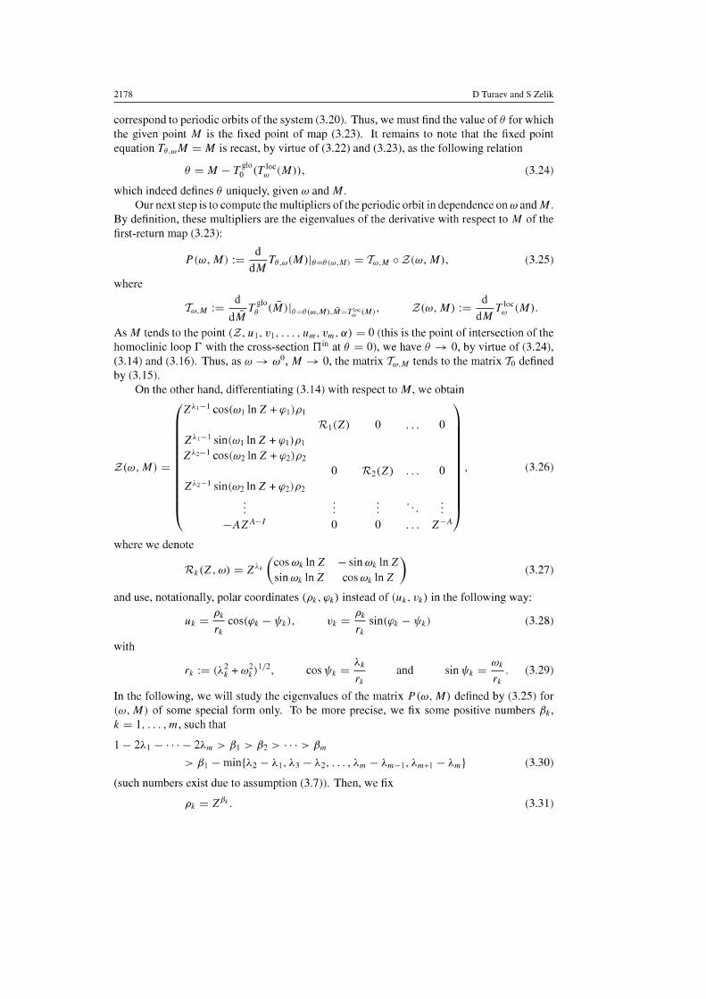
2178 D Tumev and S Zelik
correspond to periodic orbits of the system (3.20). Thus, we must find the value of 0 for which the given point M is the fixed point of map (3.23). It remains to note that the fixed point equation To . .,M = M is recast, by virtue of (3.22) and (3.23), as the following relation
0= M - Tt(T):'(M)), (3.24)
which indeed defines 0 uniquely, given W and M. Our next step is to compute the multipliers of the periodic orbit in dependence on W and M.
By definition, these multipliers are the eigenvalues of the derivative with respect In M of the first-return map (3.23):
d P(w, M) := dMTo . .,(M)lo~o(".M) = T",.M 0 Z(w, M), (3.25)
where
._ d glo - _ T",.M.- dMTo (M)lo~(",.M).M~T':-(M)'
._ d loe Z(w, M) .- dM T", (M).
As M tends to the point (Z, UI, V" ••• , Um , Vm , a) = 0 (this is the point of intersection of the homoclinic loop r with the cross-section ITm at 9 = 0), we have 0 -+ 0, by virtue of (3.24), (3.14) and (3.16). Thus, as W -+ wo, M -+ 0, the matrix T",.M tends to the matrix To defined by (3.15).
On the other hand, differentiating (3.14) with respect to M, we obtain
Z",-I cos(w,1n Z + (O,)p, 'R., (Z) 0 0
Z",-I sin(w,1n Z + (O,)p, Z",-I cos(Wz In Z + (02)P2
Z(w,M) = 0 'R.z(Z) 0 (3.26)
Z",-I sin(Wz In Z + (02)pz
_AZA-I 0 0 Z-A
where we denote
'R.k(Z, w) = Z'" (,,?SWk In Z - Sinwk In Z) smWk In Z COSWk In Z
(3.27)
and use, notationally, polar coordinates (Pk> (Ok) instead of (Uk> Vk) in the following way:
Pk Pk . Uk = - COS«(Ok - !/Ik), Vk = - sm«(Ok - !/Ik) (3.28)
'k 'k
with
and •• 1. Wk SID'Y'k =-.
rk (3.29)
In the following, we will study the eigenvalues of the matrix P(w, M) defined by (3.25) for (w, M) of some special form ouly. To be more precise, we fix some positive numbers th, k = I, ... ,m, such that
I - 2AI - ... - 2Am > {31 > {32 > ... > {3m
> {3, - min{A2 - A" A3 - A2, ... , Am - Am_I. Am+1 - Am}
(such numbers exist due to assumption (3.7)). Then, we fix
Pk = Zp'.
(3.30)
(3.31)
Homoclinic loops and dimension of attractors 2179
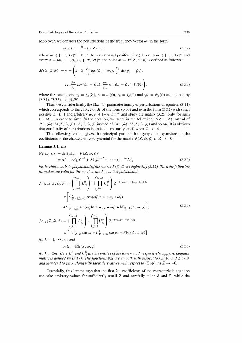
Moreover, we consider the perturbations of the frequency vector ",0 in the form
",(.0) := ",0 + (In Z)-lw, (3.32)
where .0 E [-".,3".]". Then, for every small positive Z « 1, every .0 E [-".,3".]"' and every 4> = (4)1. ... ,4>,,) E [-"., 3".]m, the point M = M(Z, .0, 4» is defined as follows:
M(Z, .0, 4» := y = (d' Z, PI COS(4)1 - 1/11), PI Sin(4)1 - 1/11), 71 71
.•. , Pm cos(4) .. - 1/1 .. ), Pm sin(4)", - 1/Im), W(O») , 7m 7m
(3.33)
where the parameters P. = p,(Z), '" = ",(.0), r, = r,(w) and 1/1, = 1/1,(.0) are defined by (3.31), (3.32) and (3.29).
Thus, we consider finally the (2m + 1) -parameter family of pertnrbations of equation (3.11) which corresponds to the choice of M of the form (3.33) and '" in the form (3.32) with srnall positive Z « 1 and arbitrary .0, 4> E [-"., 3".]m and study the matrix (3.25) only for such ("" M). In order to simplify the notation, we write in the following P(Z, .0, 4» instead of P(",(w), M(Z, .0, 4»), Z(Z, .0, 4» instead of Z(",(w) , M(Z, .0, 4») and so on. It is obvious that onr family of pertnrbations is, indeed, arbitrarily srnall when Z --> +0.
The following lemma gives the principal part of the asymptotic expansions of the coefficients of the characteristic polynomial for the matrix P(Z, .0, 4» as Z --> +0.
Lemma 3.1. Let
lI'z,,",~(/L) := det(/Lld - P(Z, .0, 4») := /Ln - Ml/Ln-l + M2/Ln-2 + ... + (_I)n Mn (3.34)
be the characteristic polynomial of the matrix P (Z, .0, 4» defined by (3.25). Then thefollowing formulae are valid for the coefficients M. of this polynomial:
M2k_l(Z, .0, 4» = (rf L~i) . (n UJi) Z-I+2I.,+ .. +2I..·,+l..+P.
]=1 ]=1
X [Ut-l,2k-l cos(",gln Z + 'Pk + .0.)
+Ut_l,2k sin(",gln Z + 'Pk + .ok) + M2k- 1 (Z, .0, 4» l (3.35)
M2k(Z, .0, 4» = (rf L~i) . (Ii UJi) Z-I+21.,+ .. +2I.,+p, J=1 J=1
X [-L~,2k sin 'Pk + L~+I,2k cos 'Pk + M 2k (Z, .0, 4» 1 fork = 1", ',m, and
~=~~,~~ ~~
for k > 2m. Here L?j and Ui~ are the entries of the lower- and, respectively, upper-triangular matrices defined by (3.17). Thefunctions ~ are smooth with respect to (.0,4» and Z > 0, and they tend to zero, along with their derivatives with respect to (.0, 4», as Z --> +0.
Essentially, this lemma says that the first 2m coefficients of the characteristic equation can take arbitrary values for sufficiently srnall Z and carefully taken 4> and .0, while the
2180 D Tumev and S Zelik
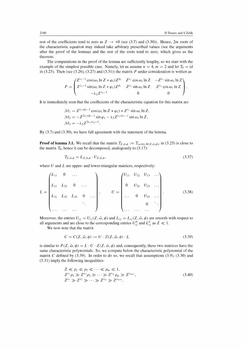
rest of the coefficients tend to zero as Z 4 +0 (see (3.7) and (3.30)). Hence, 2m roots of the characteristic equation may indeed take arbitrary prescribed values (see the arguments after the proof of the lemma) and the rest of the roots tend to zero, which gives us the theorem.
The computations in the proof of the lemma are sufficiently lengthy, so we start with the example of the simplest possible case. Namely, let us assume n = 4, m = 2 and let To = id in (3.25). Then (see (3.26), (3.27) and (3.31)) the matrix P under consideration is written as
(
Z>"-' cos(""in Z + 'P,)Zfl,
P = Z>.,-, sin(""in Z + 'P,)Zfl,
-A2Z>'2-'
Z>"cos""lnZ -Z>"Sin""inZ) Z>., sin ,,,,In Z Z>., cos ,,,,In Z .
o 0
It is immediately seen that the coefficients of the characteristic equation for this matrix are
M, = Z>',+fl,-' cos(""in Z + 'P,) + Z>., sin""in Z,
M2 = -Z2).t+J)t-lsinCPI-A2ZA2+At-lsinWllnZ,
M3 = _A2Z2J.l+).2-1.
By (3.7) and (3.30), we have full agreement with the statement of the lemma.
Proof or lemma 3.1. We recall that the matrix Tz'''.1> := T(w(").M(Z'''.I») in (3.25) is close to the matrix To, hence it can be decomposed, analogously to (3.17):
TZ,fi),t/J = LZ,(i),tP . UZ,(i),q" (3.37)
where U and L are upper- and lower-triangular matrices, respectively:
L" 0 U" U'2 U13
L2' L22 0 0 U22 U23
L= U= (3.38) L31 L32 L33 0 0 U33
0
Moreover, the entries Uij = Uij (Z, iiJ, "') and Lij = Lij (Z, iiJ, "') are smooth with respect to all arguments and are close to the corresponding entries Ui~ and L?j as Z « 1.
We now note that the matrix
C = C(Z, iiJ, "') := U . Z(Z, iiJ, "') . L (3.39)
is similar to P (Z, iiJ, "') = L . U . Z (Z, iiJ, "') and, consequently, these two matrices have the same characteristic polynomials. So, we compute below the characteristic polynomial of the matrix C defined by (3.39). In order to do so, we recall that assumptions (3.9), (3.30) and (3.31) imply the following inequalities:
Z « p, « P2 « ... « Pm « 1, Z>., p, » Z'2 P2 » ... » Z>.· Pm » Z··." (3.40) Z" » Z'2 » ... » Z" » Z>.·."
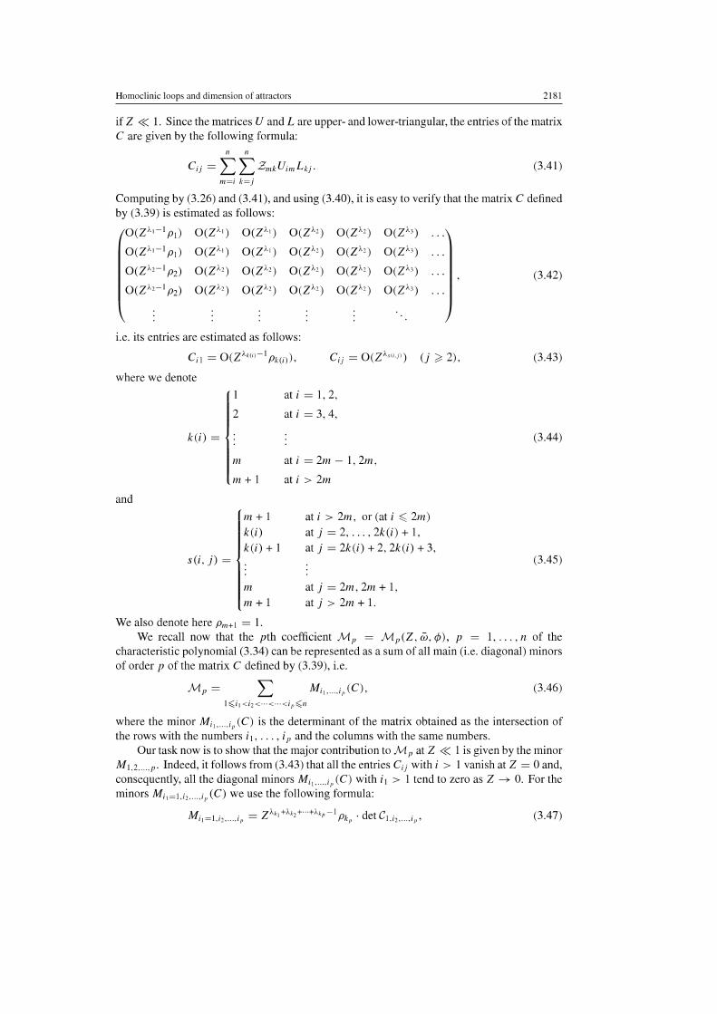
Homoclinic loops and dimension of attractors 2181
if Z « I. Since the matrices U and L are upper- and lower-triangular, the eutries of the matrix C are given by the following formula:
n n
Cij = EEZmkUimLkjo m=i k=j
(3.41)
Computing by (3.26) and (3.41), and using (3.40), it is easy to verify that the matrix C defined by (3.39) is estinJated as follows:
O(Z>.,-I PI) O(Z>") O(Z>") O(Z"') O(Z"') O(Z"')
O(Z",-I PI) O(Z"') O(Z"') O(Z"') O(Z"') O(Z"')
O(Z",-1 pz) O(Z"') O(Z"') O(Z"') O(Z"') O(Z"')
O(Z",-I pz) O(Z"') O(Z"') O(Z"') O(Z"') O(Z"')
i.e. its entries are estinJated as follows:
Cil = O(Z"·,,,-I Pk(i)) ,
where we denote
Cii = O(Z",,,·il) (j;;' 2),
I ali = 1,2,
2 ali = 3, 4,
k(i) =
m at i = 2m - I, 2m,
m+1 ali> 2m
and
m+1 at i > 2m, or (at i .;; 2m) k(i) at j = 2, ... ,2k(i) + I, k(i) + I at j = 2k(i) + 2, 2k(i) + 3,
s(i, j) =
m atj =2m,2m+I, m+1 atj>2m+1.
We also denote here Pm+ I = I.
(3.42)
(3.43)
(3.44)
(3.45)
We recall now that the pth coefficient Mp = Mp(Z, ro, 4», p = I, ... , n of the characteristic polynomial (3.34) can be represented as a sum of all main (Le. diagonal) minors of order p of the matrix C defined by (3.39), Le.
Mi, ..... i,(C), (3.46)
where the minor Mi" ... ,i,(C) is the determinant of the matrix obtained as the intersection of the rows with the numbers ii, ... , i p and the columns with the same numbers.
Ourtasknowis to show that the major contribution to M. at Z « I is given by the minor MI,2 ....... Indeed, it follows from (3.43) that all the entries Cij with i > I vanish at Z = 0 and, consequently, all the diagonal minors Mi, ..... i, (C) with il > I tend to zero as Z ~ O. For the minors Mi,~I,i" ... ,i, (C) we use the following formula:
(3.47)
2182 D Tumev and S Zelik
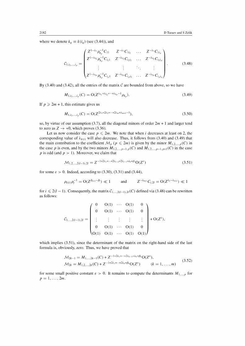
where we denote kq '" k(iq) (see (3.44)), and
Z-).lCli2
Z-Ai2; Ci2ia
(3.48)
By (3.40) and (3.42), all the entries of the matrix C are bounded from above, so we have
M· . (C) = 0(ZA.1+A.,+ .. +A.,-lp ). 1,l2 •... ,lp kp (3.49)
If p ;;. 2m + 1, this estimate gives us
(3.50)
so, by virtue of our assumption (3.7), all the diagonal minors of order 2m + 1 and larger tend to zero as Z ~ +0, which proves (3.36).
Let us now consider the case p .. 2m. We note that when i decreases at least on 2, the correspondiog value of Ak(i) will also decrease. Thus, it follows from (3.40) and (3.49) that the maio contribution to the coefficieot Mp (p .. 2m) is given by the minor Ml.2 •.... p(C) io the case p is even, and by the two minors Ml.2 ..... p_l.p(C) and Ml.2 ..... p-l.p+l (C) io the case p is odd (and p > I). Moreover, we claim that
(3.51)
for some e > O. Indeed, accordiog to (3.30), (3.31) and (3.44),
and
for i .. 2(/ - 1). Consequently, the matrix C1 ..... 2(1-ll.2l(C) defined via (3.48) can be rewritten as follows:
0 0(1) 0(1) 0
0 0(1) 0(1) 0
C1 ..... 2(1- Il.2l = +O(Z').
0 0(1) 0(1) 0
0(1) 0(1) 0(1) 0(1)
which implies (3.51), sioee the determinant of the matrix on the right-hand side of the last formula is, obviously, zero. Thus, we have proved that
M _ = M _ (C) + Z-I+2A1+··+2A.-1+A.+P·0(Z') 2k 1 1, ...• 2k 1 ,
M2k = Ml.2 •.... 2k(C) + Z-I+2A1+··+2A.+P,O(Z') (k = 1, ... , m) (3.52)
for some small positive constant e > O. It remaios to compute the determinants Ml ..... p for p = 1, ... ,2m.
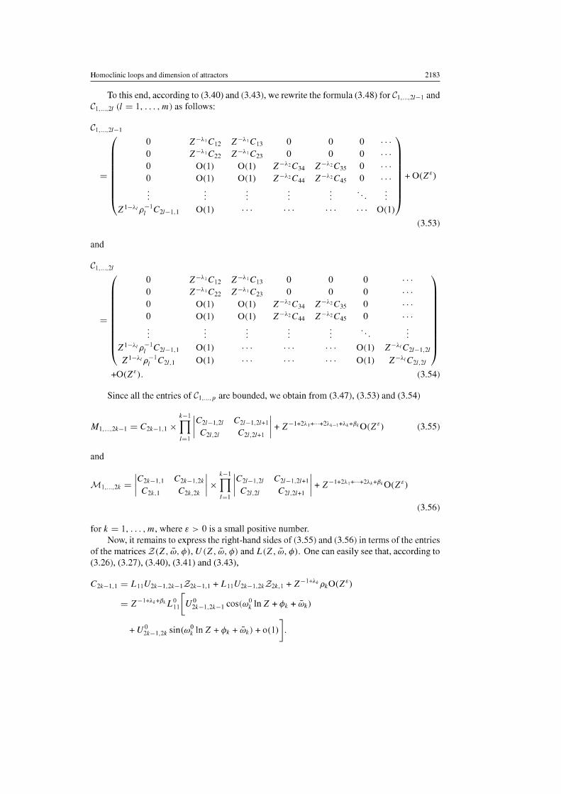
Homoclinic loops and dimension of attractors 2183
To this end, according to (3.40) and (3.43), we rewrite the formula (3.48) for CI ..... 21_1 and CI ..... 21 (I = I, ... , m) as follows:
CI ..... 21_1 0 Z-l.'CI2 Z-l.'C13 0 0 0 0 Z-l.'C22 Z-l.'C23 0 0 0 0 0(1) 0(1) Z-l.'C34 Z-l.'C35 0 0 0(1) 0(1) Z-l.'C .. Z-l.'C., 0 +O(Z')
ZI-l., -IC P, 21-1.1 0(1) 0(1)
(3.53)
and
CI ..... 21 0 Z-A1 C12 Z-AICI3 0 0 0 0 Z-l.'C22 Z-AIC23 0 0 0 0 0(1) 0(1) Z-l.'C34 Z-l.'C35 0
= 0 0(1) 0(1) Z-l.,C .. Z-l.'C45 0
ZI-AI -IC P, 21-1.1 0(1) 0(1) Z-A1C'll_I,21
ZI-l., -IC P, 21.1 0(1) 0(1) Z-l.'C2I.21
+O(Z'). (3.54)
Since all the enJries of C, •.... p are bounded, we obtain from (3.47), (3.53) and (3.54)
'-I I M = C C2I-l.21 1 ..... 2k-l 2k-l.l x n C
1=1 2l.2l
(3.55)
and
M -IC2k-I.1 1 •...• 2k - C
2k.1 C~_I.2k I x fi IC~_I.21 C~_I.21+11 + Z-I+2l.,+··+2l.,+p,O(Z')
2k,2k 1=1 21,21 21,21+1
(3.56)
for k = I, ... ,m, where. > 0 is a small positive number. Now, it remains to express the right-hand sides of (3.55) and (3.56) in terms of the enJries
of the maJrices Z(Z, w, ¢), U(Z, w, ¢) and L(Z, w, ¢). One can easily see that, according to (3.26), (3.27), (3.40), (3.41) and (3.43),
C2k- I.1 = Ll1 U2k- I.2k- IZ2k-l.l + Ll1 U2k- I.2kZ2k.1 + Z-I+l., PlOtZ')
= Z-'+l.,+P'L?1 [ U~_I.2k_1 cos(",2ln Z + ¢, + w,)
+ U~_I.2k sin(",2ln Z + ¢, + w,) + 0(1)].
2184 D Tumev and S Zelik
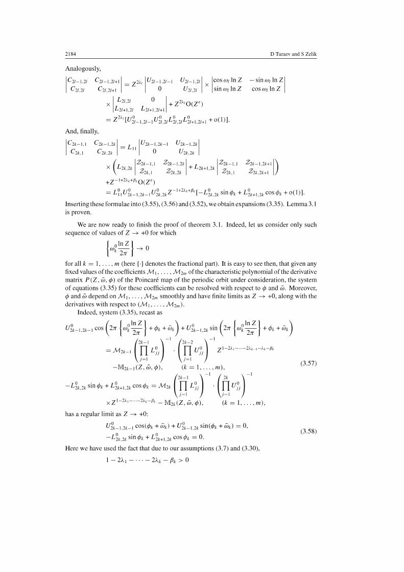
Analogously,
I
CU-l,U CU,U
CU-l,U+11 = Z2J., IUU-l,U-l UU-l,UI X I,,?SWllnZ CU,U+1 0 UU,U sm WI In Z
X I Lu,u 0 I + Z2J.'O(Z') L21+1,21 L2l+1,2l+1
= Z2J., [U~-l,U-l U~,u L~,uL~+ 1,U+ 1 + 0(1)],
And, finally,
C2k-l,2k 1 = La IU2k-l,2k-l U2k-l,2k 1
C2k,2k 0 U2k,2k
(L IZ2k-", Zu-l,2k1 + L IZu-",
X 2k,2k "'__ "'__ 2k+l,2k "' __ -lk,l -lk,2k -lk,l
+Z-1+2J.'+P'O(Z8)
-SinWllnZI cosw1lnZ
Zu-l,2k+ll) Z2k,2k+l
= L?, Ui'.-l,2k-l ui'.,2kZ-l+2J.,+p, [ -Lg.,2k sin q,k + Lg.+l,2k cos q,k + 0(1)],
Inserting these fonnulae into (3.55), (3,56) and (3,52), we obtain expansions (3.35), Lemma 3.1 is proven.
We are now ready to finish the proof of theorem 3.1. Indeed, let us consider only such sequence of values of Z -> +0 for which
{wolnZ}->o
k 2,..
for all k = I, ',., m (here (.j denotes the fractional part). It is easy to see then, that given any fixed values of the coefficients M 1, ... , M2m of the characteristic polynomial of the derivative matrix P(Z, W, q,) of the Poincare map of the periodic orbit under consideration, the system of equations (3.35) for these coefficients can be resolved with respect to q, and W. Moreover, q, and W depend on M 1, ... , M2m smoothly and have finite limits as Z -> +0, along with the derivatives with respect to (M" ... ,M2m)'
Indeed, system (3.35), recast as
Ui'.-l,2k-l cos (2,.. {w2~:} + q,k + Wk) + Ui'._l,2k sin (2,.. {w21~:} + q,k + Wk)
= M2k-l (n' L~j) -1. (n2 UJj) -1 Z'-2J.,-----2J.H-J.'-P'
}=1 J=l
-M2k_ l (Z, w, q,), (k = I, ... , m),
_ Lg.,2k sin q,k + Lg.+1,2k cos q,k = M2k (n' L ~j) -1 . (Ii UJj) -1 }=1 ]=1
xZ' -2J.,-----2J.,-P, - M2k (Z, w, q,), (k = I, ... , m),
has a regular limit as Z -> +0:
Ui'._l,2k_l COS(q,k + Wk) + Ui'._l,2k Sin(q,k + Wk) = 0,
- Lg.,2k sin q,k + Lg.+l,2k cos q,k = O.
Here we have used the fact that due to our assumptions (3.7) and (3.30),
I - 2J.., - ... - 2J..k - 13k > 0
(3.57)
(3.58)
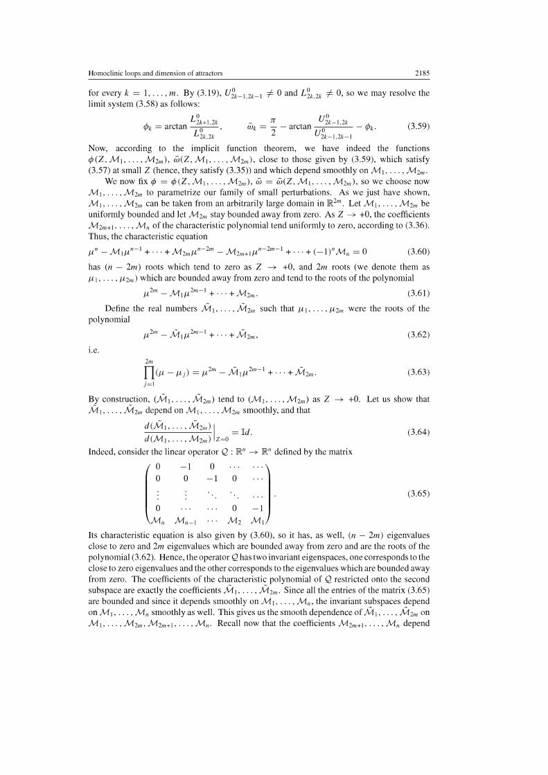
Homoclinic loops and dimension of attractors 2185
for every k = I, ... , m. By (3.19), Ul'._l 2k-l '" 0 and Lt 2k '" 0, so we may resolve the limit system (3.58) as follows: . .
Lt+l2k _ 1< Ul'.-l,2k rf>. = arctan LO " IJ). = - - arctan 0 - rf>.. (3.59)
2k,2k 2 U2k- l,2k-l
Now, according to the implicit function theorem, we have indeed the functions rf>(Z, M" ... , M2m), w(Z, M" ... , M2m), close to those given by (3.59), which satisfy (3.57) at small Z (hence, they satisfy (3.35)) and which depend smoothly on MI, ... , M2m.
We now fix rf> = rf>(Z, M" ... , M2m), w = W(Z, M" ... , M2m), so we choose now M" ... , M2m to parametrize our family of small perturbations. As we just have shown, M" ... ,M2m can be taken from an arbitrarily large domain in JR2m. Let M" ... ,M2m be unifonnly bounded and let M2m stay bounded away from zero. As Z --> +0, the coefficients M2m+l, ... , M. of the characteristic polynomial tend unifonnly to zero, according to (3.36). Thus, the characteristic equation
(3.60)
has (n - 2m) roots which tend to zero as Z --> +0, and 2m roots (we denote them as IL" ... , IL2m) which are bounded away from zero and tend to the roots of the polynomial
(3.61)
Define the real numbers M" ... , M2m such that IL" ... , IL2m were the roots of the polynomial
(3.62)
i.e.
(3.63) j=l
By construction, (MI,"" M2m) tend to (MI, ... , M2m) as Z --> +0. Let us show that M" ... , M2m depend on M" ... , M2m smoothly, and that
d(M" ... , M2m) I = lId. (3.64) d(M" ... ,M2m) Z~O
Indeed, consider the linear operator Q : JR' --> JR' defined by the matrix
o o
o
-I o
o -I 0
o -1 M. M.-l M2 M,
(3.65)
Its characteristic equation is also given by (3.60), so it has, as well, (n - 2m) eigenvalues close to zero and 2m eigenvalues which are bounded away from zero and are the roots of the polynomial (3.62). Hence, the operator Q has two invariant eigenspaces, one corresponds to the close to zero eigenvalues and the other corresponds to the eigenvalues which are bounded away from zero. The coefficients of the characteristic polynomial of Q restricted onto the second subspace are exactly the coefficients M" ... , M2m. Since all the entries of the matrix (3.65) are bounded and since it depends smoothly on M" ... , M., the invariant subspaces depend onM", .. , M. smoothly as well. This gives us the smooth dependence of M" ... , M2m on M" ... , M2m, M2m+" ... , Mo. Recall now that the coefficients M2m+l, ... , M. depend
2186 D Tumev and S Zelik
on (M" ... , M2m) smoothly, and they are continuous in Z along with the derivatives with respect to (M!. ... , M2m). Thus, the required smooth dependence of M" ... , M2m on (M" ... , M2m) at all small Z, including Z = 0, follows inunediately. Identity (3.64) follows now from the fact that (M" ... , M2m) = (M" ... , M2m) at Z = O.
Now, by implicit function theorem, we have that given any values M" ... ,M2m with M2m oF 0, the corresponding values of M" ... , M2m are defined uniquely. In turn, the coefficients M I, ... , M2m are defined uniquely by (3.63), given any (symmetric with respect to the complex conjugation) set"R- of the non-zero roots /101, ••• , /102m. Hence, given any such set "R-, we find the corresponding values of M" ... , M2m, and then the values of the perturbation parameters </> and W, for arbitrarily small values of Z. Theorem 3.1 is proven.
By taking in theorem 3.1 the values of the multipliers /101, ••• , /102m outside the unit circle, we arrive at the following corollary.
Corollary 3.1. Let the assumptions of theorem 3.1 hold. Then, by an arbitrarily small COO-perturbation of system (3.1), a periodic orbit P the instability index N+(P) of which satisfies
(3.66)
can be bom in an arbitrarily small neighbourhood of the homoclinic loop under consideration.
Remark 3.2. We note that the unstable manifold WU(P) of the periodic orbit P constructed in corollary 3.1 has dimension 2m + 1. Thus, if every solution of the perturbed system (3.20) can be extended globally for positive t E JR., then this unstable manifold is, obviously, a (2m + I)-dimensional invariant submanifold for the system under consideration. Moreover, due to remark 3.1, we have
dim WU(P) = [dimdA)l, (3.67)
where [v 1 denotes the integral part of v. Since such invariant manifolds always belong to the attractor (if the system possesses a global attractor) then corollary 3.1 and formula (3.67) present a possibility of obtaining lower bounds for the attractor's dimension in terms of their Lyapunov dimension. This possibility will indeed be used in the next section in order to obtain sharp lower bounds for the attractor's dimension for the abstract hyperbolic equation (1.1).
It is also interesting to consider the case where the multipliers /101, ••• , /102m in theorem 3.1 are all equal to I in the absolute value. In this case, a small perturbation of the periodic orbit P with the multipliers /101, ••• , /102m can produce an (m + I)-dimensional invariant torus (see a proof in appendix B). This gives us the following corollary.
Corollary 3.2. Let the assumptions of theorem 3.1 hold. Then, by an arbitrarily small COO-perturbation of system (3.1), an (m + I)-dimensional smooth invariant torus, densely filled by a quasi-periodic trajectory. can be bom in an arbitrarily small neighbourhood of the homoclinic loop under consideration.
4. Lower bounds for the dimension or the attractor
In this concluding section, we obtain sharp lower bounds for the attractor's dimension for the damped hyperbolic equation (1.1) with the noulinesrity in the class § (see definition 2.2). The main result here is the following theorem.
Homoclinic loops and dimension of attractors 2187
Theorem 4.1. Let A : D (A) --> H be any linear self·adjoint operator whose eigenvalues satisfy (2.1), and let (e;}~1 be the corresponding orthonormal system of eigenvectors. Then there exist two smooth nonlinear operators IF, and IF 2 in the form
lFi(u) := Fl((u, ell, (u, e2))e, + Fi2((u, ell, (u, e2))e2, u E H, i = 1,2 (4.1)
(where F/ E C8"(IR2, IR), i, j = 1,2) and a smoothing operator <I> = <I>,.y.k.m defined for every e > 0, every small y > 0 and every k, m E 111, belonging to the class S and satisfying the estimate
1I<I>lIcl(E~,"') :;;; e,
such that the fractal dimension of the anractor A = Ay.,.k.m of the equation
at2u + yatu + Au = IF, (u) + ylF2(u) + <I>(u, atu)
possesses the following estimates:
1 dim A 1 c,-:;;; p( ,E):;;; C2-, Y Y
where the positive constants C, and C2 are independent ofy, e, k and m.
Proof. First, take a second order ODE in the form:
at2u = U - FoCU), U E IR,
(4.2)
(4,3)
(4.4)
(4.5)
where Fo E C""CIR) vanishes at the origin together with its first derivative. We assume that equation (4.5) possesses a homoclinic orbit Uo (t) to the equilibrium U = 0 (as an example, take FoCU) = U3 ). Let us fix a sufficiently small y > 0, n := [l/(2y)]- 1 and a frequency vector '" := ("", .. , , w,) E IR' and consider the following decoupled system of second order ODEs:
at2U(t) = U(t) - Fo(U(t)),
at2u, (t) + yatu, (t) + ",iu, (t) = 0,
(4.6)
at2il. (t) + yatu. (t) + ",~u. (t) = O.
By construction, this system has a homoclinic loop of the type studied in section 3, so one can expect an analogue of theorem 3.1 for the perturbations of system (4.6), as is indeed given by the following lemma.
Lemma 4.1. Let the above assumptions hold and let, in addition, y
"'i > 2' for every i = 1,,,., n. (4.7)
Then, for every e > 0 and every k E 111, there exist C8"-functions <l>i IROn+2 --> IR, i = 0, 1, ... , n, satisfying
lI<I>dlcl(lR"'.'.lI<) :;;; e, such that the system
at2U(t) = U(t) - Fo(U(t)) + <l>o(U(t), atU(t), u(t), atil(t)),
at2u, (t) + yatu, (t) + ",iu, (t) = <1>, (U(t), atU(t), u(t), atu(t)),
at2u.(t) + yatU.(t) +",~u.(t) = <I>.(U(t) , atU(t), u(t), atu(t)),
possesses a periodic orbit P with the instability index N+(p) = 2n.
(4.8)
(4.9)
2188 D Tumev and S Zelik
Proof. Let us introduce new variables z(t) := U(t) + O,U(I) , w(t) := U(I) - O,U(I) ,
2 2 U,(I):= U,(I), V,(I):= (",?)-I (O,U,(I) + ~U,(t)),
where",? := (",y - y2/4)1/2 > 0, i = I, ... , n. In these variables, system (4.6) reads
o,z=z- ~Fo(z+w), o - Y - 0-UtUl = -2:U1 + lOi VI,
0- y - 0-tVt = -2:V1 - WI"!,
o - y - 0-Ut U" = -2:un + WnVn '
0- y - 0-(1,Vn = -2:vn - Wn"",
o,w = -w+~Fo(z+w).
(4.10)
(4.11)
Note that system (4.11) has the form of (3.1) and that all assumptions of theorem 3.1 are, obviously, satisfied. Consequently, according to this theorem, for every given 8 > 0 and kEN, there are Co-functions ci>, : IR2n+2 --> IR, i = 0, ... , 2n + I, satisfying
llci>dlc/OR""'.IR) .;; 8, (4.12) such that the following pertorbation of system (4.11)
o,z = z - ~Fo(z + w) + ci>o(z, w, u, iJ),
o - Y - 0- 11>- ( --) UtUj = -2:"; + wi Vi + 2i-l Z, W, u, v ,
0- y - 0- 11>- ( --) IJtVi=-2:Vi-WjUi+ 2iZ,W,U,V,
o,w = -w + ~ Fo(z + w) + ci>2n+1 (z, w, ii, v),
(4.13) i = 1, ... ,n,
possesses a periodic orbit P with the instability index N+(P) = 2n. This periodic orbit lies in a small neighbourhood of the homoclinic loop of the unperturbed system, so we may assume without loss of generality that all the functions ci>, have finite supports.
It remains to rewrite system (4.13) as a system of second order ODEs for the variables U(t) := z(t) + w(l) and u,(t). To this end, we take the sum of the first and last equations of (4.13) and differentiate it with respect to 1 and, analogously, we differentiate the equations for U,(I) in (4.13). This gives us
o,2U(I) = U(I) - Fo(U(I» + ci>o(Z(I), w(I), ;;(1), v(t»,
0,2;;,(1) + yo,;;,(I) + ",;U,(/) = ci>,(Z(/) , w(/), ;;(/), v(/)),
where the Co functions ci>, : IR2n+2 --> IR satisfy
i = 1, . .. ,n, (4.14)
llci>dlcZ-'(R"'-'.IR) .;; Ck 8 (4.15)
and the constant C. is independent of 8. Th finish the proof of the lemma, it remains to express the variables z, w, ih in terms of U, BtU, ii j and atu; from the system z+w = U,
z - w = BtU - ci>o(z, w, ii, v) - <l>2n+l (z, W, ii, v),
- (0)-1 (0 - y - ) (0)-111>- ( --) Vj = It)j Ut"j + 2:Uj - Wi 2i Z. W, u, v .
(4.16)
i = 1, . .. ,n.
Homoclinic loops and dimension of attractors 2189
Note that in the case where all ci>i are equal to zero ideutically, system (4.16) reduces to a non-degenerate linear system. Hence, due to (4.12), the system of equations (4.16) can indeed be solved in a unique way (by virtue of the implicit function theorem) if e is small enough:
z = eo(U, a,u, ii, a,ii),
Vi = 8 i(U, atu, u, atu),
w = e.+I(U, a,u, ii, a,ii)
i = 1, ... ,n, (4.17)
for some Coo-functions ei, i = 0, ... , n. Inserting (4.17) into the right-hand side of (4.14) finishes the proof of lemma 4.1.
Let us now finish the proof of theorem 4.1. Indeed, let A be a self -adjoint positive operator in a Hilbert space H with a compact inverse, such that its eigenvalues 0 < AI"; A2";'" satisfy condition (2.1) for a certain positive constant K. Let (ei }~I be the corresponding orthonormal system of eigenvectors. Then, every H-valued function u(t), t E JR., can be expanded as follows:
00
u(l) := L ui(t)ei, ui(l) := (u(I), ei). (4.18) i=1
Moreover, due to (1.2), 00
S E lR. (4.19) i=1
We rewrite now equation (4.3) in the following eqnivalent form: 2 -
at Ui(l) +yatUi(l) +Aiui(l) = <l>i(u(I), a,u(I», i = 1,2, ... , (4.20)
where u(l) = (UI(I), U2(t), ... ) E !Roo (see (4.18» and (ci>i(U, a,u)}~1 are defined as
ci>i(U, a,u) := (l1'\(u) + ylF2(U) + <I>(u, a,u), ei). (4.21)
We will construct the desired equation (4.3) in the form (4.20). The main idea is to construct the nonlinearities in such a way that the components Ui (t) of the corresponding solution will satisfy system (4.9). Then, by lemma 4.1, this equation will possess a periodic orbit P such that N+(P) = 2n, n + I := [1/(2y)] and, consequently, the fractal dimension of its attractor will be larger than (2y)-I. Indeed, let y > 0, e > 0 and let kEN be arbitrary. Let us also fix n := [i/(2y)]-1 as in lemma 4.1. We need to rewrite system (4.9) constructed in lemma 4.1 in the form (4.20). To this end, we fix the frequencies w? = Ai+2, i = I, ... , n, where Ai are the eigenvalues of A, and introduce the variables
uI(I) := U(t), u2(1) := a,U(I), u,(I) := UI (I), ... ,
In these variables, system (4.9) is written as follows:
at2UI + yatul + AIUI = (UI - Fo(ul) + Alu1I
+Y{U2} + <1>1 (Ul, ... , Un+2, atU!, ... , atUn+2),
Ot2U2 + YOtU2 + A2U2 = {U2 - F~(UI)U2 + A2U2}
+y{UI - Fo(ul)} + <l>2(UI. ... , U.+2, OtUI, ... , O,U.+2),
Ot2U3 + yatU3 +).3U3 = <l>3(Ul, ... , Un+2, atU!, ... , OtUn+2),
u.+2(1) := u.(I).
(4.22)
(4.23)
2190 D Tumev and S Zelik
where the C8"-functions <l>i satisfy
lI<I>dlc'-'(ll~'.lR) :;;; C~.. (4.24)
Since every solution of (4.9) is, obviously, a solution of (4.23) as well, system (4.23) also has a periodic orbit P with N+(P) = 2n.
We complete system (4.23) as follows:
i = n + 3, n + 4, .... (4.25)
Then, system (4.23) and (4.25) has the form (4.20) indeed. Moreover, since only the existence of a periodic orbit P with N+(P) = 2n is important for our purposes, we may cut off all the nonlinearities outside this orbit and define finally
and
Ul - FO(Ul) + A1UI
U2 - F6(Ul)U2 + A2U2
o o
IF2(U) := </>0 •
<I>(U, Otu) := <l>n+2(UI, ... , Un+2, atUl, ... , Bt Un+2)
o o
where </>0 := </>0 (lUI 12 + IU212) is an appropriate cut-off function.
(4.26)
(4.27)
Thus, the desired operators IF 1, IF 2 and <I> are defined. Let us now verify that they satisfy all conditions of theorem 4.1. Indeed, (4.1) is obvious. Since the operator <I> has a finite rank (see (4.27)), then, obviously, <I> E S. Moreover, it follows from (2.1), (4.19) and (4.24) that, for every mEN
1I<I>lIc'-'(E--.H'") :;;; Cn"".. (4.28)
Hence, by rescaling, if necessary, ., we may always satisfy (4.2) (for every fixed m). Furthermore, due to our construction, system (4.23) and (4.25) possesses a saddle periodic orbit P with N+(P) = 2n. Therefore,
dimF(A. E) ~ 2n ~ --'-. 2y
(4.29)
The upper bounds for the fractal dimension in (4.4) is an immediate corollary of proposition 2.1 and corollary 2.2. Theorem 4.1 is proven.
Remark 4.1. We emphasize that the operators IF 1 and IF 2 from theorem 4.1 have a very simple structure (see (4.26)) and can be computed explicitly. It is also worth to emphasize that the unpertorbed system (4.3)
Ot2U + YOtU + Au = IFI (u) + yIF2(u)
possesses a four-dimensional inertial manifold
M := {(Uh U2, OtUl, OtU2) E IR4, (Ui, OtUi) = 0, i = 3, 4, ... J
(4.30)
Homoclinic loops and dimension of attractors
and, consequently, the fractal dimension of its attractor Ao satisfies
dim.(Ao, E) .;; 4, for every y > 0,
whereas its Lyapunov dimension, obviously, satisfies
dimL(Ao, E) ~ y-I.
2191
(4.31)
(4.32)
Theorem 4.1 shows, however, that we may drastically increase the fractal dimension of the attractor A by an arbitrari1y small perturbation of equation (4.30), and achieve
dim. (A, E) ~ dimL(A, E) ~ y-I. (4.33)
This example confirms that the Lyapunov dimension is a more robust qualitative characteristic of the global attractor than its fractal dimension.
Remark 4.2. We have constructed in theorem 4.1 the examples of attractors A of equations of the form (1.1) which depend explicitly on the first derivative atu of the unknown function u. Differentiating, however, equation (4.3) by t and denoting v = atu and wet) := (u(t), vet»~ E
ii: := H x H, we obtain the equation of the form
at2w + yatw +Aw = F\(w) + y1F2 (w) + <i>(w), (4.34)
where the nonlinearities are already independent of at w. Therefore, the phenomena described in theorem 4.1 can appear in hyperbolic equations of the form (1.1) where the nonlinearity F is independent of at u (F (u, atu) '" F (u». Unfortunately, this reduction leads to linear opemtors A in a special form
- (A 0) A:= ° A . (4.35)
In order to avoid this restriction, we permit the explicit dependence of the nonlinearity F on atu in our abstract model (1.1).
We recall that the usual way of obtaining lower bounds for an attractor's fractal dimension is to estimate the instability index for some equilibrium of the equation under consideration, see [1,2] and references therein (see also [27], where lower estimates for the instability index of a linear non-autonomous equation of type (1.1) with periodic coefficients were given based on the parametric resonance phenomena). In our next proposition, we show that it is, in principle, impossible, using this method, to obtain reasonable lower bounds for the attractor's dimension of equation (1.1) with nonlinearities belonging to S.
Proposition 4.1. Let A be a linear self-adjoint operator with a compact inverse in a Hilbert space H whose eigenvalues satisfy (2.1) and let the nonlinearity F in equation (l.1) belong to the class S. Then, for every 8 > 0, there exists a positive constant C, such that the instability index of any equilibrium Uo of equation (1.1) is estimated asfollows:
(4.36)
Proof. Indeed, due to the trick described in remark 4.2, it is sufficient to prove estimate (4.36) only for the case where
F(u, atu) '" F(u). (4.37)
Let now Uo be an arbitrary equilibrium of equation (1.1). Then, the corresponding equation of variations reads
at2w + yatw +A.,w = 0, A., := A - F' (uo) (4.38)
2192 D Tumev and S Zelik
and, consequently, the spectrum of the linearization D.oS, of the semigroup (1.7) at the point (uo, 0) can be expressed as follows:
u(D.oS,) = {e'/4, I"~ := _~ ± (:2 _ ek) 1/2} , (4.39)
where {ek}k:,l E C are the eigenvalues of the operator A.o'
We recall now that the operator F belongs to the class S. Therefore,
IIF' (uo) 1I.c(H-.II'") .;; Cm (4.40)
for every mEN, where the constant Cm is independent of Uo E H. Thus, due to the classical theory of compact perturbations of self-adjoint operators (see, e.g., [28]), we derive from (4.40) that for every N E N, there exists a constant CN such that
lek - Akl .;; CNk-N, kEN,
where Ak are the corresponding eigenvalues of the unperturbed operator A. It follows that all but finitely many ek have positive real parts, and their iruaginary parts tend to zero faster than any power of k as k --> +00. Hence, according to formula (4.39), the number of eigenvalues I"~ with non-negative real parts satisfies (4.36) indeed. Proposition 4.1 is proven.
Remark 4.3. We stress that our 'homoclinic' method of obtaining lower estimates for the attractor's dimension gives, in fact, more than an estimate from below of the maximal attractor. Indeed, in absolutely the same way as theorem 4.1 was deduced from corollary 3.1 to theorem 3.1, we obtain from corollary 3.2 that the noulinearities Il'\2 and <I> can be constructed in such a way that equation (4.3) would have an invariant torus of dimension ~C / y, where C is a certain constant, densely filled by quasi-periodic trajectories (at y = 0 this system may be integrable, nevertheless all its invariant tori are killed at non-zero y due to the way we introduce the dissipation in our examples; hence, the invariant torus which we obtain is of a different nature).
In other words, we show that equations under consideration may have minimal sets whose dimension is of the sarne order as the Lyapunov dimension of the maximal attractor. Recall also that, according to [29], any quasi-periodic flow on a smooth (m + I)-dimensional invariant torus can be pertorbed in such a way that the torus would contain an invariant m-dimensional manifold, homeomorphic to Dm- l x Sl, the flow on which is smoothly conjugate to a suspension over any aforehand given diffeomorphism of Dm-l. Hence, by corollary 3.2, every dynamics which is possible in a phase space of dimension ~C /y can be encountered in equation (4.3), after an appropriate choice of the noulinearities.
Aeknowledgments
This research was partially supported by INTAS project no 00-899 and CRDF grant no 10545. We are also grateful to Messoud Effendiev who introduced us to each other.
Appendix A. Proof of theorem 1.1 and lemma 2.1
In this appendix, we prove the existence of a solution for problem (1.1) under the assumptions of theorem 1.1. We also prove the Lipschitz property of the corresponding semigroup S" as well as the quasi-differentiability of S, on the attractor A (lemma 2.1). As usual (see [I], [3] chapter 4 and [4]), the proof is done via the Galerkin approximation method, based on the a priori estimates (1.6), (1.8) and (1.9).
Homoclinic loops and dimension of attractors 2193
We start with the proof of the a priori estimate (1.6). Let ~ E c(lR,., E) be a solution of (1.1). Then, according to assumption (1.4), the nonlinear term F(u, o,u) belongs to the space c(lR,., H) and is globally bounded in it. Consequently, we may take a scalar product of equation (1.1) with O,U(I) + aU(I), where a > 0 is a sufficiently small number, and derive the following relation (see, e.g., [3], lemma 11.4.1):
~o,[lIo,u(l) II~ + lIu(t) II~, + 2a(u(t), o,u(t))] + (y - a) lIo,u(t) II~ + allu(t)lI~
= (F, u + ao,u) :;;; c, + 8(lIo,U(I)II~ + 1lu(t)1I~,), where 8 > 0 can be arbitrarily small. Fixing now 8 « I and a « I in the last inequality and applying Gronwall's inequality, we obtain (1.6) indeed.
Let us now verify estimate (1.8). Let ~., (I) and ~'2 (I) be two solutions of (1.1) and let ~(I) := [v(I), o,v(I)] := ~,(I) - ~2(1). Then v(t) satisfies the following equation:
O,2v +yo,v +Av = L,(I)v +L2(I)O,v, ~I,~o = ~,(O) - ~2(0), where
and
L2(t) := /.' F~,.(su, + (I - S)U2, so,u,) ds.
We note that, according to (1.4), these operators are globally bounded as operators from H' --> H and H --> H, respectively. Consequently, the right-hand side of the equation for v belongs to the space C(lR,., H) and we may take a scalar product of this equation with o,v and derive the following estimate:
~[lIo,v(l) II~ + IIV(I)II~,] + y II O,V (I) II~
= (L,(t)v(t), o,v(t)) + (L2(t)O,V(t), o,v(t)) :;;; K(lIv(t)II~, + lIo,v(t)II~),
where K is independent of u, and U2 (since the derivatives F. and F~,. are assumed to be globally bounded). Applying Gronwall's inequality to this relation, we obtain (1.8).
In order to prove the a priori estimate (1.9), let us differentiate equation (1.1) with respect to 1 and introduce the function z(l) := O,u(I). Then, this function satisfies the following equation:
O,2Z + yo,z + Az = F~(u, o,u)z + F~.(u, o,u)o,z,
zlt~ = u~, o,zl,~o = o;u(O) = -Auo - yu~ + F(uo, u~). (A. I)
Denote ~(t) := [z(I), o,z(t)]. Since HO) := [u(O), o,u(O)] E E' and the nonlinearity F satisfies (1.4), it follows that ~(O) E E and
II~(O)II~:;;; C(IIHO)II~, + I) (A.2)
for an appropriate constant C depending on F and y. Moreover, it follows from estimate (1.6) and from equation (1.1) that
1I~(t)II~-, :;;; C'II~(O)II~e-Y' + C;, (A.3)
where C' and C; depend only on A, F and y. Taking the inner product in H of equation (A.I) with the function o,z(t) + (y/2)z(t),
we have
o'{lIo,zll~ + IIzII~, + y (z(t), o,z(l))) + y lIo,zll~ + y IIzll~, = 2(F~(u, o,u)z, o,z) + 2(F~.(u, o,u)o,z, o,z)
+y(F~(u, o,u)z, z) + y(F~.(u, o,u)a,z, z). (A.4)
2194
Using conditions (1.5), we derive that
2(F~(u, o,u)z, o,z) + 2(F~ •• (u, o,u)o,z, o,z)
:s;; ~(lIo,z(l) II~ + IIz(l) II~,) + 4Cy II [z(I), o,z(I)]II~_,. Analogously, using assumption (1.4) on the derivatives of F, we estimate
D Tumev and S Zelik
(A.5)
(F~(u, o,u)z, z) + (F~ •• (u, o,u)o,z, z) :s;; i(lIo,z(I)II~ + IIZ(I)II~,) + C'II[Z(I), o,z(I)]II~_,. (A.6)
Inserting estimates (A.5) and (A.6) into the right-hand side of(A.4), we obtain, for a sufficiently small Y > 0,
o,{lIo,zll~ + IIzll~, + y(Z(I), o,z(l))} + ~(lIo,zll~ + IIzll~, + y(Z(I), o,z(l))} :s;; C;II~(I)II~_, for an appropriate constant C; which depends only on y, A and F. Applying here Gronwall's inequality, and using (A.2) and (A.3), we arrive at the estimate
II~(I)II~:S;; C.e-Y'/811~(0)1I~, + C.. (A.7)
It remains to note that due to equation (1.1) and condition (1.4) we have
IIW)II~, :s;; c(1I~(t)II~ + I),
so (1.9) follows from (A.7). Now we can prove the existence of the solutions of (1.1). Let {e.}~, be the orthonormal
basis in H generated by the eigenvectors of the self-adjoint operator A and let ITN be an orthoprojector to the first N eigenvectors in H, HN := ITNH and EN := ITNE. For every N E N, we consider the following problem in the finite-<limensional space EN, which approximates the initial infinite-dimensional problem (1.1):
O,2UN + YO/UN +AUN = ITNF(UN, O/UN),
~N(I) := [UN(t) , O,UN(I)] E EN, ~N(O) = ~~. (A.S)
We recall that (ITNF, VN) = (F, VN) for every VN E EN and, consequently, repeating word by word the derivation of estimates (1.6) and (1.9), we obtain the following uniform (with respect to N) a priori estimates for the solutions of (A.S):
I. II~N(t)II~:S;; CII~N(O)IIEe-Y' + C" (A.9)
where the constants C, C" C2 and C, are the same as in (1.6) and (1.9) (and, in particular, they are independent of N). On the other hand, equation (A.S) is a system of ODEs with smooth (C l ) nonlinearity and, consequently, estimates (A.9) give the global existence of a solution ~N(I) E EN of problem (A.S). Our task now is to pass to the limit N --> 00 in (A.S) and construct the solution u(l) of (1.1) as a limit of Galerkin solutions UN(I). To this end, we first assume that the initial conditions ~ (0) for problem (1.1) belong to E':
HO) EE' and set ~~ := ITNHO). (A.lO)
Then, according to (A.9)(2) and equation (A.S), we have the uniform with respect to N estimate
IIO;UN IILOO([O.T].H) + II~N IILoo([o.T].E'l :s;; C(IIHO) liE')' (A.ll)
which is valid for every T > O. Consequently, without loss of generality, we may assume that, for every T > 0,
~N --> ~ *-weaklyin L""([O, T],E'),
*-weakly in L ""([0, T], H) (A. 12)

Homoclinic loops and dimension of attractors 2195
forsomefunction~ := [u, atu] E L""(~, EI). We claim that u solves the initial problem (1.1). To this end, we need to pass to the limit N --> 00 in equations (A.8). Indeed, passing to the limit N --> 00 in the linear tenns of (A.8) is evident due to (A. 12). In order to pass to the limit in the nonlinear term, we recall that the embedding
L""([O, T], E) n (a;u E L""([O, T], H)} c C([O, T], E)
is compact, for every T > 0 (see, e.g., [3], chapter 4) and, consequently, (A.12) implies the strong convergence ~N --> ~ in C([O, T], E). Since the operator F is continuous, it follows that fIN F(UN, atUN) --> F(u, a,u), and u is indeed a solution of problem (1.1).
Thus, forevery~(O) E E', wehaveconstructedasolution~ E L""(~, E') nC(~, E) of problem (1.1) (moreover, arguing in a standard way as, e.g., in [3], chapter 4, one may verify that ~ E C(~, E'), in fact). It is not difficult now to extend this result to the initial data from E. Indeed, let ~ (0) E E be an arbitrary initial condition. Let us consider a sequence ~n (0) E E' such that
~n (0) --> HO) asn ..... 00. (A. 13)
Let also ~. (t) E E' be the corresponding solutions of problem (1.1), the existence of which has just been proven. Then, according to estimate (1.8), there exists some function ~ E C~, E) such that
in C([O, T], E) strongly (A. 14)
for every T > O. As above, the strong convergence law (A.14) allows us to pass to the limit n --> 00 in the equations for u' and verify that the limit function u(t) also satisfies equation (1.1). Thus, the existence of a solution of problem (1.1) is now proven under the assumptions of theorem 1.1.
It remains to prove the quasi-differentiability of the corresponding semigroup St on the attractor A. Let~, (t) and ~2(t) be two solutions of problem (1.1) belonging to A and let v(t) be a solution of equation of variations (2.7) (computed along the trajectory ~,(t)) with [v(O), a,v(O)] = ~,(O) - MO). Then, arguing as in the derivation of estimate (1.8), we obtain the following estimate:
lI[v(t), a,v(t)]lIi ~ CII[v(O), a,v(O)]lIieK', (A. IS)
where the constants C and K are independent of u, and U2. Moreover, the function w(t) := u, (t)-U2(t)-V(t) obviously satisfies thefollowinglinearnon-homogeneous equation
where
a,2W + ya,w +Aw - F~(u), a,u,)w - FL(u)' a,u,)a,w = h .... ,(t),
[w, a,w]I,~o = 0,
h .... ,(t) := {J.' (F~(su, + (I - S)U2' sa,u,) - F~(u), a,u,) ds} v(t)
+ {J.' (F~.(su, + (I - S)U2, sa,u,) - F~(u), a,u,) dS} a,v(t).
Consequently, analogously to (1.8) and (A. IS), we have
lI[w(T), a,w(T)]IIE ~ CeKT J.T IIh., .• ,(t)lI~dt,
(A. 16)
(A. 17)
(A. 18)
where the constants C and K are independent of u, and U2. On the other hand, since the attractor A is compact in E, the set
A'.2 := {s~, + (I - s)b ~" ~2 E A, s E [0, III
2196 D Tumev and S Zelik
is also compact in E and, due 10 assumption (1.4), the derivatives F~ and F~. are uniformly continuous on this set. Consequently, we have an estima10
(A. 19)
where the function a (z) tends to zero as z --> 0+ and is independent of t, uland U2.
Estimates (1.8), (A. 15), (A. 18) and (A.19) imply that
lI[w(T), atw(T)lll~';; aTm,(O) - MO)IIE)II~,(O) - MO)IIE, (A.20)
where the function aT (z) tends 10 zero as z --> 0+, it depends on T ;;. 0 but it is independent of ~" ~2 E A. Thus, estima10 (2.2) is verified. The continuity of S' (~) on the attractor is verified analogously. End of the proof.
Appendix B. Proof of coroUary 3.2
Let P be a periodic orbit, born by a small perturbation of a homoclinic loop of sys10m (3.1), which has 2m multipliers equal to I in absolute value (such an orbit can indeed be born according to theorem 3.1). Let us prove that a smooth (m + l)-dimensioual invariant Iorus, filled by quasi-periodic trajectories each of which is dense in the torus, can be born at the bifurcations of P.
Consider a Poincare map (x t-+ x) for the periodic orbit P:
x = Bx +o(x), (B. I)
here x = 0 is the fixed point which corresponds to the orbit P. The eigenvalues of the matrix B are the multipliers of P. By assumption, 2m of these eigenvalues lie on the unit circle. Our goal is 10 prove that this map can be perturbed in such a way that an m-<limensional invariant torus would appear in a small neighbourhood of the origin.
Fix any integer 7 ;;. I. It is obvious that, by perturbations, small in C' -topology, one can arrange arbitrary small changes in any entries of the matrix B in (B.I). Hence, we can always achieve that B would have exactly m pairs of complex-conjuga1o eigenvalues on the unit circle: e±w" ... , e±w.., all OJ are rationally independent and the factors OJ j /n are irratioual; and the rest of the multipliers does not lie on the unit circle.
By the centre manifold theorem, our map has a 2m-dimensional smooth invariant manifold which is tangent at x = 0 10 the eigenspace of B corresponding 10 the multipliers on the unit circle. It is well-known that since the numbers {n, OJ" ••• , w",} are rationally independent, there exist local coordiuates (Zl, ... ,Zm) E em in which the map on the centre manifold takes the following (normal) form:
Zj = Qj(ZlZr, ... ,ZmZ~)Z+o(z') (j = I, ... ,m), (B.2)
where' means complex conjugation, and Qj are complex polynomials of degree';; (7 - 1)/2,
~~=~. (B~ It is obvious that by an arbitrary small (in the C' -topology) perturbation, one can make map (B.2) coincide with the polynomial map
(j = I, ... ,m) (B.4)
in a sufficiently small neighbourhood of zero. Thus, it is enough to prove that a small perturbation of map (B.4) can produce an m-dimensioual invariant torus arbitrarily close to Z = O.
Let us, first, introduce polar coordiuates pje'·} := Zj, j = I, ... , m. Map (B.4) can be recast as
(j = I, ... ,m) (B.5)
Homoclinic loops and dimension of attractors 2197
where Qj '" Rje"'! (j = I, ... , m), so Rj, OJ are real analytic functions, and
(j = I, ... ,m). (B.6)
Let ai, ... , am, 91, ... , 9m be arbitrary small numbers. Then the map
Pj = (aj + Rj(p~, ... , p;'»Pj' 'Pj = <pj + OJ + OJ(p~, ... , p;,) (j = I, ... , m)
(B.7)
is a small (real analytic) perturbation of (B.5). The amplitude map
Pj = (aj + Rj(pt, ... , p;'»Pj (j = I, ... , m) (B.8)
is independent here of the phases <PI. ... ,<Pm' Therefore, a fixed point of (B.8) with all PI. ... , Pm non-zero corresponds to an m-dllnensional invariant torus of (B.7).
Take now some sufficiently small strictly positive numbers pr, ... , p~. Put
aj = 1- Rj «pr)2, ... , (p~)2), OJ = "'j - OJ((pr)2, ... , (p~)2) (j = I, ... , m).
(B.9)
By (B.6), the numbers a" ... , am, 0" ... , Om are indeed small when pr, ... , p~ are small. With a" ... ,am given by (B.9), (pr, ... , p~) is a fixed point of (B.8), i.e. the torus (p, = pr, ... , Pm = p~) is a smoothm-dimensional invariant torus of (B.7). By construction, map (B. 7) is a C' -small perturbation of the restriction of the original Poincare map on the centre manifold, so we have indeed constructed the perturbation under which an invariant torus is born from our periodic orbit. By (B.6) and (B.7), the restriction of the Poincare map on this torus is given by
'Pj = <pj + "'j (j = I, ... , m).
Since the numbers 1f, "'" ••• , Wm are mtionally independent, it follows that every orbit of this map is indeed quasi-periodic and fills the torus densely. End of the proof.
References
[1] Babin A and VlShik M 1989 Attractors of Evolutionary Equations (Moscow: Nauka) [2] Hale J 1987 Asymptotic Behavior of Dissipative Systems (Math. Surveys and Monographs vol 25) (Providence,
RI:AMS) [3] TemamR 1997 Infinite DimensionalDynamicalSystems in Physics andMechanics 2nd edn(New York: Springer) [4] Chepyzhov V and Vtshik M 2002 Attractors for Equations of Mathematical Physics (Providence. RI: AMS) [5] Kaplan L and Yorke J A 1979 Functional Differential Equations and Approximation of Fixed Points (Lecture
Notes in Mathematics vol 730) (Berlin: Springer) pp 204-27 [6] Constantin P and Foias C 1985 Global Lyapunov exponents. Kaplan-Yorke formulas and the dimension of the
attractors for 2D Navier-Stokes equations Commun. Pure Appl. Math. 38 1-27 [7] Douady A and Oesterli J 1980 Dimension de Hausdorff des attracteurs C. R. Acad. Sci. Paris A 290 1135-8 [8] Hunt B 1996 Maximum local Lyapunov dimension bounds the box dimension of chaotic attractors Nonlinearity
, 845-52 [9] Blinchevskaya M and nyashenko Yu 1999 Estimate for the entropy dimension of the maximal attJactor for
k-contracting maps in an infinite dimensional space Russ. J. Math. Phys. 6 20-6 [10] Chepyzhov V and nyin A 2001 A note on the fractal dimension of attractors of dissipative dynamical systems
Nonlin. Anal. Theory Methods Appl. 44A 811-9 [11] Sell G 1989 Hausdorff and Lyapunov dimension for gradient systems Contemporary Math. 99 85-92 [12] Shilnikov L 1965 A case of the existence of a countable number of periodic motions Sov. Math. Dokl. 6 163-6 [13] Shilnikov L 1970 A contribution to the problem of the structure of an extended neighborhood of a rough
equilibrium state ofsaddle-focus type Math. USSR, Sb. 10 91-102 [14] Afrajmovich V. Bykov V and Shilnikov L 1983 On structurally unstable attracting limit sets of Lorenz attractor
type 'ITans. Mosc. Math. Soc. 1983 153--216 [151 Shilnilrov A, Shilnilrov L and Turaev D 1993 Normal forms and Lorenz attractors Biji",'" Chao,3 1123-39
2198 D Tum .. and S Zelik
[16] Turaev D and Shilnikov L 1998 An example of a wild straoge attractor Sb. Malh. 189 137-60 [17] Turaev D 1996 On dimension of non-local bifurcational problems Bifurca. Chaos 6 123--56 [18] Li Y. McLaughlin D, Shatah J and Wtggins S 1996 Persistent homoclinic orbits for a perturbed nonlinear
SchrOdinger equation Commun. Pure AppL Math. 49 1175-255 [19] Li Y 1999 Smale horseshoes and symbolic dynamics in pertUIbed nonlinear Schrodinger equation J. Nonlinear
Sci. , 363-415 [20] ShatahJ andZeng C 2000 Homoclinic orbits for the perturbed sine-Gordon equation Commun. Pure AppL Math.
53 283--99 [21] Shatah J and Zeng C 2000 Homoclinic orbits for a perturbed nonlinear Schrtklinger equation Commun. Pure
AppL Math. S3 1222-83 [22] Gbidaglia J and Temam R 1987 Attractors for damped nonlinear hyperbolic equations J. Malh. Pure AppL 66
273-319 [23] Feireisl E 1995 Global att.ra.ctors for semilinear damped wave equations with supercritical exponentJ. Dig. Eqns
116431-47 [24] Triebel H 1978 Interpolation Theory, Functional Spaces, Differential Operators (Amsterdam: North-Holland) [25] Shilnikov L, Shilnikov A. Turaev D and Chua L 1998 Methods of Qualitative Theory in Nonlinear Dynamics
part I (Singapore: World Scientific) [26] Sternberg S 1958 On the structore of local homeomorphisms of Euclidean .-space II Am. J. Malh. 80 623-31 [27] Zelik: S 1997 The Mathieu-Hill operator equation with dissipation and estimates for its instability index Math.
Notes 61451--64 [28] Ghohberg I and Krein M 1969 Introduction to the Theory of Linear Non-selfadjoint Operators in Hilbert Space
(Providence. RI: AMS) (translated from Russian) [29] Newhouse S, Ruelle D and Takens F 1978 Occurrence of strange Axiom A attractors near quasi-periodic flows
on TIfJ, m ~ 3 Commun. Math. Phys. 64 35-40


![Belyakov Homoclinic Bifurcations in a Tritrophic Food Chain …math.bd.psu.edu/faculty/jprevite/REU07/yu.pdf · dT Dl] , (2.lc) where T is time, R and K are prey intrinsic growth](https://static.fdocuments.us/doc/165x107/5f4b0977817bbb35cd4c7834/belyakov-homoclinic-bifurcations-in-a-tritrophic-food-chain-mathbdpsuedufacultyjprevitereu07yupdf.jpg)