TEAM PROJECT 1

GEO-DEMOGRAPHIC ANALYSIS OF THE HOME DEPOT INC.

AT POSTAL ZIP CODE LEVEL

PREPARED FOR

DATA-DRIVEN MARKETING DECISIONS, FALL 2016

(MIGB 7732)

Prepared by

Abhishek Nithyananda Shetty

Kehan Wang

Puneet Gangrade

Yijun Liu

30 September 2016

EXECUTIVE SUMMARY

Not only the square-footage growth of an organization but also the best customer experience

drives productivity and efficiency. 61% of the firms spending the most on marketing did not

have a defined and documented process to screen, evaluate, and prioritize marketing

campaigns and 82% of the firms never tracked and monitored marketing campaigns and

assets using automated software such as marketing resource management (MRM) (Mark

Jeffery, 2010) 1 .

The Home Depot, a home improvement supplies superstore, operates in a highly competitive

industry against Lowe’s and other rivals and is here to win by providing the best customer

experience and gaining valuable insights about individual-level customer data. The Home

Depot is making sure that stores are easy to locate, merchandise selection is easy, high-level

service is available, and the products are there at the lowest price.

This study provides the Geo-Demographic Analysis at Postal Zip Code level data for The

Home Depot in Texas. The investigation uses the data made available from one of the

datasets of Wharton Research Data Services (WRDS). The Direct Marketing Educational

Foundation (DMEF) Academic Zip Data Set of WRDS provides the demographic

information of people living in Texas. The study incorporates the Hierarchical Cluster

Analysis to analyze the data set. This method of cluster analysis seeks to build a hierarchy of

groups.

The report features most appropriate zip code areas of Texas for providing discounts and

flexible payments on home improvements or renovation projects. Using this list, the

ii

marketing department will be able to devise its future marketing campaigns to maximize

sales for dedicated customer segments. With the help of insights achieved from this analysis,

Home Depot will be able to embrace the demographic and psychographic changes in the

markets. Eventually, it will be able to gain the trust of customers and become the game

changer in Texas. The executive concern of Home Depot is to increase its market share and

market attractiveness in Texas.

iii

TABLE OF CONTENTS

1. Introduction………………………………………………………………………......1

1.1 Status Quo………………………………………………………………………..1

1.2 Previous Researches……………………………………………………………...1

1.3 Problem Statement…………………………………………………………….....2

1.4 Objective……………………………………………………………....................2

1.5 Report Structure……………………………………………………………….…2

2. Background……………………………………………………………......................3

2.1 Overview……………………………………………………………...................3

2.2 Target Customer……………………………………………………………........3

2.3 SWOT Analysis……………………………………………………………........4

2.4 Competitors Analysis……………………………………………………………5

2.5 Campaign Introduction………………………………………………………….8

3. Methodology and Data Analysis……………………………………………………8

3.1 Variable Definition……………………………………………………………..9

3.2 Methods…………………………………………………………………….…10

3.3 Analysis…………………………………………………………………….…11

3.3.1 Ward's Method. ……………………………………………………..11

3.3.2 Furthest Neighbor Method…………………………………………..12

4. Recommendations……………………………………………………………………..18

5. Conclusion……………………………………………………………………………...20

6. Limitations and Future Research……………………………………………………….22

7. Bibliography……………………………………………………………………………24

8. Appendices……………………………………………………………………………..25

iv

1. INTRODUCTION

1.1 STATUS QUO

57% of the companies did not use a centralized database to track and analyze their marketing

campaigns, and 43% of the companies did not use metrics to guide future marketing

campaign selection and management. Are companies neglecting the impact that data can have

on their marketing decisions? It is an interesting fact that only 20% of the companies who

make data-driven marketing decisions are the leaders in the market (Mark Jeffery, 2010) 2 .

The housing industry tends to be highly cyclical since trends in the home improvement

industry (of $325 billion)3 are highly correlated with that of the housing market.

Unprecedented adverse change has characterized the market for home building products in

the past several years. Companies who have managed to adapt and thrive have done so by

keeping a close watch on the market and industry during these hard times.

1.2 PREVIOUS RESEARCHES

Researchers have found some effective ways for companies to remodel the homes (Nino

Sitchinava, 2015)4, as well as how to overcome barriers to innovation in the home-

improvement marketplace (W. Chan Kim, 1999)5. But they failed to figure out which

segment of customers tends to spend more money on home renovation. Thus, keeping up-to-

date on customers’ behavioral patterns is critical to capitalize on trends and to avoid losing

customers.

1

1.3 PROBLEM STATEMENT

Although Home Depot has earned $78 billion as

annual sales and gained 24% market share (Great

Speculations, 2015)6 in the United States as a

whole, it has not been able to capture the market

share in the state of Texas due to fierce competition from Lowe’s. Despite having 179 stores

as compared to Lowe’s 141 stores, Home Depot was incapable to gain a larger share-of-

wallet. This report evaluates this problem and provides feasible solutions through preliminary

data analysis and some recommendations to develop effective promotion campaigns.

1.4 OBJECTIVE

This study has been undertaken at the request of the Vice President of Home Depot to

identify the most appropriate zip code areas for running the promotional campaign for

providing discounts and flexible payments on home improvement and renovation. The

ultimate goal of Home Depot is to increase its market share and retain the existing customers.

When the insights gained from this study are implemented, the Home Depot stands to earn a

firm stance in the market and become the preferred choice for all people who are looking to

improve their homes by purchasing tools, construction products, and services.

1.5 REPORT STRUCTURE

This report seeks to explore the following research question in the context of shifts in the

home renovation industry: Which customer segments and zip code areas of Texas would be

ideal for Home Depot to deploy marketing strategies?

This study examines the data set by using IBM’s statistical software package SPSS. The

report is structured as follows:

2

1. Analyze the strengths and weaknesses of the Home Depot, and the opportunities and

threats from its competitors and macro-environment by using SWOT analysis.

2. Use Ward’s Method and Squared Euclidean Distance measure to conduct geo-

demographic cluster analysis.

3. Present the data-based chart and the analysis of the results and offer key findings

about the analysis as well as major recommendations for launching effective

promotions.

4. The report concludes with a discussion of the implications, limitations, and

suggestions for future research.

2. BACKGROUND

2.1 Overview

Arthur Blank and Bernie Marcus founded Home Depot in Atlanta, Georgia, in 1978. Since

then, it has managed to grow into the country’s largest retailer in home improvement

business. Home Depot’s mission is to excel in customer satisfaction by consistently selling

high quality products, customer service, and competitive pricing. The company strives for the

customer to get the best possible service by training skilled employees and nurturing long

lasting relationships with customers.

2.2 Targeted customer

Home Depot’s customers are mainly homeowners, general contractors, tradesmen, repairmen,

and small business owners. The average age of a Home Depot shopper is 50, and the

customers’ annual average income is $60,8007. However, it has categorized its customers into

3 groups: Do-It-Yourself, Do-It-For-Me, and Professional Customers:

3

• The Do-It-Yourself customers are the homeowners who purchase the required products to

complete their projects and repairs by themselves

• The Do-It-For-Me customers are the homeowners who purchase their products and hire a

third party to complete their repairs and projects. To these customers, Home Depot is able

to offer its installation programs on carpeting, countertops, water heaters, roofing, and

many others

• The professional customers are mainly general contractors, repairmen, and small business

owners. Home Depot offers numerous services to these customers to make their shopping

experience better by assisting them with dedicated staff, designated parking, and bulk

pricing

2.3 SWOT Analysis

Strengths

• Diversified product and service portfolio

• Strong brand image

• Multi-Channel selling

• Sustained financial growth

Weaknesses

• Huge debt

• Lower inventory turnover ratio

• Limited supply chain

Opportunities

• Expanding retail market in the US

• Focus on customer-centric business model

• Growth in online purchasing

• The female customers

Threats

• Expansion by competitors

• Highly conditional on the performance

of the U.S. economy

4

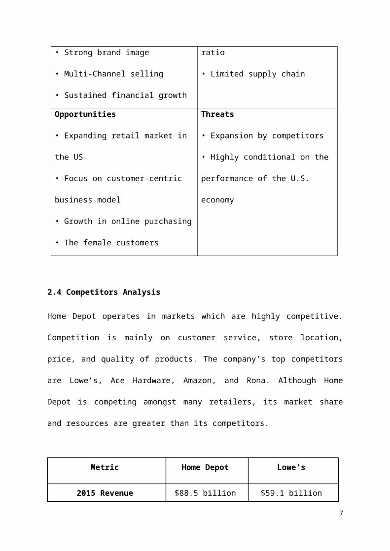
2.4 Competitors Analysis

Home Depot operates in markets which are highly competitive. Competition is mainly on

customer service, store location, price, and quality of products. The company's top

competitors are Lowe’s, Ace Hardware, Amazon, and Rona. Although Home Depot is

competing amongst many retailers, its market share and resources are greater than its

competitors.

Metric Home Depot Lowe's

2015 Revenue $88.5 billion $59.1 billion

2015 Net Profit $7.0 billion $2.5 billion

% Increase Over 2014 10.5% -5.6%

Comparable-Store Sales Growth 5.6% 4.8%

Profit Margin 7.9% 4.3%

Figure 2.1 Direct Competitor Comparison

5

Key Success Factor

Importance

Weight Home Depot Lowe’s Ace Hardware

Relative Product Price 0.30 8 2.4 7.5 2.25 5 1.5

Brand

Image/Recognition 0.20 9 1.8 7 1.4 3 0.6

Executive Management 0.05 8 0.4 8 0.4 5 0.25

Use of Technology 0.10 7 0.7 8 0.8 3 0.3

Distribution Network 0.20 9 1.8 8 1.6 10 2

Financial Resources 0.15 9 1.35 7 1.05 5 0,75

Sum of Important

Weights 1.00

Weighted Overall

Strength Rating 8.45 7.5 5.4

Figure 2.2 competitive strength assessment

6

Figure 2.3 Strategic Group Map

Figures 1 and 2 states the competitive strength assessment that Home Depot is the best

positioned company in this industry and Lowe’s is not far behind Home Depot. The major

difference between Home Depot and Lowe’s was Home Depot’s advantage in financial

strength and possessing a powerful brand.

From Figure 3, Home Depot and Lowe‘s own an overlapping piece of the market. Ace

Hardware is much smaller than the two main competitors and sells its products at a higher

price point.

7

2.5 Campaign Introduction

To increase its market share in Texas, Home Depot is planning to execute a campaign to offer

discounts and flexible payments on the home improvement projects to its potential customers.

This campaign will attempt to attract the homeowners who belong to the age group of 35-54

and have an average annual income of $60,800.

3. METHODOLOGY AND DATA ANALYSIS

This segment discusses the variables used and the key methods followed to achieve the

primary objectives of identifying the suitable zip codes for promotional campaigns. For the

in-depth analysis, this study examined the respective data set obtained from Direct Marketing

Educational Foundation (DMEF) Academic Zip Data Set. The data set comprises of various

parameters such as income, age, education, family size, etc. belonging to 1,964 different zip

codes across Texas.

8

3.1 Variable Definition

The below mentioned variables help us divide the customers into groups with homogeneous

needs and response patterns:

Variable Name Definition Rational Target/Reasons

prchhfm Percentage of Households in Texas that are families

Families in Texas having their own homes

Research suggests that majority of the families invest in home interior shopping on a frequent basis

prc3554 Percentage of people belonging to the age group of 35-54 in occupied households

Age Category Based upon the secondary data sources, the average age of consumers buying furniture is 50. So, in order to maximize its brand awareness and market share in Texas, it will be a wise decision to target people in the age group of 35-54

cemi Estimated median income in thousands of dollars (as of 1995)

Income Income helps in broadly classifying the customer segments to understand their purchasing capability.

prcowno Percentage of people with own households

People living in their own homes.

People living in their own homes have a higher potential to buy furniture or renovate their homes. This variable is effective for formulating promotional campaigns.

9

3.2 Methods

As this study explores a relatively small data set, Hierarchical Cluster Analysis is the most

appropriate method for analyzing the data. This Agglomerative Hierarchical Clustering start

by defining each data point to be a cluster and combine existing clusters at each step. Under

this analysis, Ward's and Furthest Neighbor are the preferred methods to investigate this data

set.

Fig 1.1 - Flowchart Representation of Cluster Analysis

10

3.3 Analysis

3.3.1 Ward's Method:

To distinguish the zip codes for the promotional campaigns, the study uses the hierarchical

cluster analysis for investigating the data set. After examining the data, the variables are

standardized using Z-Scores. Standardization is very important as the cluster variable Cemi

value (median income) is comparatively large, making the variance be significantly different

between the variables. To get a better understanding of the target customer segment and to

classify segments of similar size, the study opts for Ward's as the primary method for data

analysis and selects Squared Euclidean as the measure of distance. Squared Euclidean is

favored for standardized data because it is relatively faster than Euclidean and it gives more

preference towards variables that are distant from each other.

By following the Agglomeration table (Appendix A) and analyzing the respective

coefficients, there is a gradual difference in the values represented in the graph across 3 and 5

clusters. The values plateau and remain almost stable after the sixth cluster, so a range of 3-6

clusters is feasible for the analysis. In the first stage of analysis, Cluster 3 and 4 (Appendix B)

have similar results. As compared to cluster 4, cluster 5 is a viable option to target the ideal

customer segment. But, it cannot be the preferred cluster as it consists of an extensive zip

code range. After further examining cluster 5 and cluster 6 (Appendix B), it is observed that

cluster 6 is the best solution. Cluster 6 aligns with the primary goal of targeting the specific

set of zip codes having high percentage of owner-occupied houses, families, a healthy

percentage of people in the age group of 35-54, and an average median income for an

effective marketing campaign.

Taking into consideration the variables mentioned above, the two prominent segments in this

11

cluster are as follows:

1. First choice - target customers with estimated median income of $61,000

2. Second choice - target customers with estimated income of $93,000

Table 1: Ward’s Method - Cluster 6: Priority 1 ( Table 5 - yellow) , Priority 2 (Table 6 -

red)

3.3.2

Furthest

Neighbor

Method

The second

approach is

Furthest

Neighbor

method. This method is preferred to identify a small group of niche customer segment, for

example, highly profitable customers. After interpreting and understanding the agglomeration

table (Appendix C), the range of 3-6 clusters is selected. By comparing cluster 3 and 4

(Appendix D), cluster 4 is a better option as it matches with majority of the variables except

for median income, which is on the higher side. After further investigation of cluster 4,

cluster 5, and cluster 6 (Appendix E), even though the results look promising, they fail to

target the average median income of $61,000 which is a key parameter for the analysis.

Conclusion: After examining both the methods, cluster 6 under the Ward's method with 214

zip codes (Table 3.1) is the most appropriate customer segment for desired promotional

12

 Variables

Ward Method

1 2 3 4 5 6Mea

nCount

Mean

Count

Mean

Count

Mean

Count

Mean

Count

Mean

Count

% HH that are Families

38 51 70 452 65 183 78 991 81 214 85 63

prc3554 29.16

51 28.63

452 35.87

183 37.08

991 47.18

214 56.90

63

Current Estimated Median Income in 000s

47 51 32 452 55 183 37 991 61 214 93 63

%OOHH

19 51 74 452 46 183 75 991 73 214 81 63

                  Priority 1 Priority 2

campaigns.

Table 3.1 Final list of 214 zip codes

Case Summary Zipcode Population PostOfficeName County prchhfm

Cemi prcowno

prc3554

78747 3070 AUSTIN TRAVIS 81 93 79 4177586 15046 SEABROOK HARRIS 69 90 62 5078871 69 LANGTRY VL VERDE 67 89 67 3775229 27621 DALLAS DALLAS 75 88 78 3877401 13913 BELLAIRE HARRIS 68 85 75 4276051 30774 GRAPEVINE TARRANT 77 84 67 5278735 3463 AUSTIN TRAVIS 79 83 79 5278232 27332 SAN ANTONIO BEXAR 76 80 73 5078734 7495 AUSTIN TRAVIS 76 80 72 4277066 23310 HOUSTON HARRIS 80 78 69 5176248 13235 KELLER TARRANT 87 77 84 5176021 31798 BEDFORD TARRANT 66 77 53 4976126 14301 FORT WORTH TARRANT 84 77 81 4775044 30455 GARLAND DALLAS 77 76 72 5475007 43554 CARROLLTON DALLAS 78 76 68 5178258 2877 SAN ANTONIO BEXAR 90 76 84 4875010 4379 CARROLLTON DALLAS 75 76 68 3676017 42829 ARLINGTON TARRANT 78 75 71 4875115 33750 DESOTO DALLAS 82 74 73 5175002 24151 ALLEN COLLIN 87 74 81 4877505 10978 PASADENA HARRIS 82 74 73 4876429 127 CADDO STEPHENS 71 74 83 3077071 21037 HOUSTON HARRIS 70 73 55 4877476 794 SIMONTON FT BEND 82 73 84 4676012 24141 ARLINGTON TARRANT 75 73 64 4675080 37227 RICHARDSON DALLAS 78 73 69 4475181 5005 MESQUITE DALLAS 87 73 94 4179077 51 SAMNORWOOD CLNGSWTH 82 73 85 3175039 598 IRVING DALLAS 67 72 35 63

77380 16541THE WOODLANDS

MONTGMRY 76 72 61 52

78266 2058 SAN ANTONIO BEXAR 87 72 90 4977904 18465 VICTORIA VICTORIA 80 72 72 4676123 5314 FORT WORTH TARRANT 87 72 86 4578413 27278 CORPUS CHRSTI NUECES 73 72 54 4576001   ARLINGTON TARRANT 85 72 86 4476571 3454 SALADO BELL 80 72 82 3775087 17438 ROCKWALL ROCKWALL 81 71 76 50

13

78023 3566 HELOTES BEXAR 81 71 87 4975088 21041 ROWLETT DALLAS 88 71 89 4777382   SPRING HARRIS 86 71 91 4277089 37678 HOUSTON HARRIS 82 70 70 5277571 31556 LA PORTE HARRIS 82 70 73 4877084 45762 HOUSTON HARRIS 75 70 57 4877064 21388 HOUSTON HARRIS 78 70 69 4678736 5812 AUSTIN TRAVIS 78 69 77 5377040 30761 HOUSTON HARRIS 73 69 63 5076177 152 FORT WORTH TARRANT 95 69 90 4975048 5632 GARLAND DALLAS 88 69 82 4777566 24000 LAKE JACKSON BRAZORIA 81 69 72 4675052 40458 GRAND PRAIRIE DALLAS 83 68 77 5077493 10088 KATY HARRIS 84 68 71 5076179 15236 FORT WORTH TARRANT 84 68 77 4979121 3454 AMARILLO POTTER 77 68 73 4877573 28900 LEAGUE CITY GALVESTN 79 68 73 4775067 46151 LEWISVILLE DENTON 74 68 63 4676018 15590 ARLINGTON TARRANT 85 68 86 4079705 27708 MIDLAND MIDLAND 75 68 67 4076502 15632 TEMPLE BELL 74 68 65 4077469 31170 RICHMOND FT BEND 82 67 72 4976063 17381 MANSFIELD TARRANT 86 67 81 4977976 517 NURSERY VICTORIA 90 67 86 4978660 10986 PFLUGERVILLE TRAVIS 85 67 79 4878249 19127 SAN ANTONIO BEXAR 77 67 73 4878727 14276 AUSTIN TRAVIS 77 67 68 4677449 22664 KATY HARRIS 82 67 74 4577043 21042 HOUSTON HARRIS 75 67 58 4476133 44032 FORT WORTH TARRANT 75 67 68 4078681 17196 ROUND ROCK WILLMSON 87 66 75 5477083 37446 HOUSTON HARRIS 79 66 63 5477373 33118 SPRING HARRIS 84 66 69 5377532 18293 CROSBY HARRIS 83 66 77 4775006 37699 CARROLLTON DALLAS 71 66 55 46

77302 5767 CONROEMONTGMRY 87 66 84 45

79424 22873 LUBBOCK LUBBOCK 71 66 65 4178254 1340 SAN ANTONIO BEXAR 83 65 84 5075074 29591 PLANO COLLIN 79 65 68 49

79366 1248RANSOM CANYON LUBBOCK 85 65 88 48

77041 14790 HOUSTON HARRIS 80 65 77 4778253 3861 SAN ANTONIO BEXAR 82 65 87 4777375 19801 TOMBALL HARRIS 79 65 70 4677521 33895 BAYTOWN HARRIS 78 65 65 4679423 17308 LUBBOCK LUBBOCK 79 65 74 4679124 3342 AMARILLO POTTER 78 65 77 45

14

78748 16288 AUSTIN TRAVIS 80 65 67 4476002   ARLINGTON TARRANT 86 65 88 4378414 8600 CORPUS CHRSTI NUECES 72 65 61 4377489 27760 MISSOURI CITY FT BEND 87 64 83 6377411 678 ALIEF HARRIS 86 64 71 5675043 46620 GARLAND DALLAS 75 64 60 5075104 19503 CEDAR HILL DALLAS 85 64 81 4977581 20565 PEARLAND BRAZORIA 82 64 73 4676180 44496 FORT WORTH TARRANT 78 64 66 4477065 15867 HOUSTON HARRIS 73 64 55 4478610 7487 BUDA HAYS 87 63 83 5278260 1684 SAN ANTONIO BEXAR 83 63 90 5277562 8773 HIGHLANDS HARRIS 80 63 79 42

75234 25992FARMERS BRNCH DALLAS 70 63 63 39

75249 8677 DALLAS DALLAS 87 62 77 59

77385 7311 CONROEMONTGMRY 88 62 86 53

78250 43845 SAN ANTONIO BEXAR 86 62 77 5278628 14100 GEORGETOWN WILLMSON 82 62 71 4978504 15183 MC ALLEN HIDALGO 82 62 71 4875154 16882 RED OAK ELLIS 86 62 78 4776712 14756 WACO MCLENNAN 79 62 65 4677866 373 MILLICAN BRAZOS 79 62 83 4479912 46537 EL PASO EL PASO 71 62 59 4178163 3956 BULVERDE COMAL 84 61 88 5478247 25418 SAN ANTONIO BEXAR 78 61 71 5277336 6529 HUFFMAN HARRIS 84 61 81 4976148 22794 FORT WORTH TARRANT 86 61 80 4777031 14021 HOUSTON HARRIS 68 61 47 4678239 21781 SAN ANTONIO BEXAR 80 61 71 4376065 10271 MIDLOTHIAN ELLIS 84 60 76 4975056 22549 LEWISVILLE DENTON 86 60 77 4875166 510 LAVON COLLIN 82 60 86 4875173 1594 NEVADA COLLIN 82 60 86 4875116 18023 DUNCANVILLE DALLAS 80 60 66 4879380 374 WHITHARRAL HOCKLEY 84 60 85 4376137 15226 FORT WORTH TARRANT 80 60 80 4379084 2858 STRATFORD SHERMAN 83 60 72 42

77384 1635 CONROEMONTGMRY 85 59 87 50

78374 15498 PORTLAND SAN PATR 82 59 67 4978045   LAREDO WEBB 90 59 81 4876015 14544 ARLINGTON TARRANT 76 59 59 4679036 4853 FRITCH HUTCHNSN 89 59 91 4578148 13215 UNIVERSAL CTY BEXAR 79 59 50 4575098 15418 WYLIE COLLIN 83 59 82 4476134 17442 FORT WORTH TARRANT 81 59 77 44

15

75097 258 WESTON COLLIN 81 59 84 4476008 5300 ALEDO PARKER 85 58 84 4977396 16151 HUMBLE HARRIS 82 58 70 4877477 19232 STAFFORD FT BEND 76 58 56 4876014 26087 ARLINGTON TARRANT 77 58 56 4878359 332 GREGORY SAN PATR 84 58 62 4475040 45359 GARLAND DALLAS 83 58 76 4475150 51494 MESQUITE DALLAS 73 58 59 4475078 1103 PROSPER COLLIN 79 58 74 4376548   HARKER HGHTS BELL 80 58 58 4277086 16075 HOUSTON HARRIS 82 57 58 5276643 8487 HEWITT MCLENNAN 84 57 66 5178634 2314 HUTTO WILLMSON 81 57 80 4878725 2764 AUSTIN TRAVIS 84 57 85 4777099 38397 HOUSTON HARRIS 69 57 42 4777441 1740 FULSHEAR FT BEND 79 57 80 4678410 20860 CORPUS CHRSTI NUECES 82 57 65 4579119 968 AMARILLO POTTER 86 57 84 4576052 1105 HASLET TARRANT 86 57 76 4478233 36334 SAN ANTONIO BEXAR 81 56 68 5075121 437 COPEVILLE COLLIN 82 56 86 4977088 44595 HOUSTON HARRIS 78 56 64 4878619 1064 DRIFTWOOD HAYS 83 56 77 4877386 8379 SPRING HARRIS 82 56 67 4678418 19749 CORPUS CHRSTI NUECES 75 56 56 4679012 352 BUSHLAND POTTER 83 56 89 4678613 21272 CEDAR PARK WILLMSON 84 56 79 4579713 793 ACKERLY DAWSON 82 56 68 4477049 14445 HOUSTON HARRIS 81 55 69 5275791 8273 WHITEHOUSE SMITH 86 55 84 4777431 8 DANCIGER BRAZORIA 84 55 89 4676564 229 PENDLETON BELL 85 55 78 4579236 174 GUTHRIE KING 83 55 36 4477015 42008 HOUSTON HARRIS 74 55 59 4478109 13291 CONVERSE BEXAR 86 54 75 5378244 13798 SAN ANTONIO BEXAR 86 54 81 5075232 28289 DALLAS DALLAS 80 54 77 5077657 10791 SILSBEE HARDIN 82 54 80 4677530 23408 CHANNELVIEW HARRIS 81 54 71 4576579 3562 TROY BELL 83 54 77 4578641 10367 LEANDER WILLMSON 84 54 83 4575462 15302 PARIS LAMAR 83 54 80 4577447 5040 HOCKLEY HARRIS 82 54 67 4477578 4754 MANVEL BRAZORIA 82 53 86 4977072 41808 HOUSTON HARRIS 74 53 44 4976036 8749 CROWLEY TARRANT 80 53 71 4677632 13790 ORANGE ORANGE 82 53 79 4578642 2028 LIBERTY HILL WILLMSON 82 52 83 53

16

76140 17658 FORT WORTH TARRANT 83 52 80 4776028 33535 BURLESON JOHNSON 84 52 80 4677510 11098 ALTA LOMA GALVESTN 82 52 82 4677565 4399 KEMAH GALVESTN 69 52 60 4577085 6519 HOUSTON HARRIS 82 51 73 5476539 3884 KEMPNER LAMPASAS 88 51 81 5379932 14909 EL PASO EL PASO 85 51 71 5076227 3089 AUBREY DENTON 80 51 79 4777626 1451 MAURICEVILLE ORANGE 83 51 92 4678245 23993 SAN ANTONIO BEXAR 83 51 69 45

78132 6412NEW BRAUNFELS COMAL 85 51 86 45

76467 286 PALUXY HOOD 88 50 84 4977044 10612 HOUSTON HARRIS 80 50 72 4878041 46156 LAREDO WEBB 87 50 62 4776259 1443 PONDER DENTON 82 50 78 4676655 4007 LORENA MCLENNAN 87 50 84 4475485 399 WESTMINSTER COLLIN 85 50 84 4477045 22141 HOUSTON HARRIS 84 49 76 5779936 51666 EL PASO EL PASO 85 49 76 4779376 30 TOKIO TERRY 83 49 66 4777038 15653 HOUSTON HARRIS 77 48 53 4778362 5871 INGLESIDE SAN PATR 80 48 60 4677862 855 KURTEN BRAZOS 87 48 83 4477050 3709 HOUSTON HARRIS 85 47 81 5779935 20465 EL PASO EL PASO 78 47 55 5177053 20720 HOUSTON HARRIS 85 45 72 5978719 5368 AUSTIN TRAVIS 82 45 72 4977577 2023 LIVERPOOL BRAZORIA 80 45 73 4678724 6465 AUSTIN TRAVIS 83 44 70 4878409 2655 CORPUS CHRSTI NUECES 80 44 74 4877039 23839 HOUSTON HARRIS 84 42 66 5078595 3351 SULLIVAN CITY HIDALGO 80 39 58 5377048 13873 HOUSTON HARRIS 80 39 64 5277078 12357 HOUSTON HARRIS 84 38 67 5376070 206 NEMO SOMERVEL 76 37 69 4776077 722 RAINBOW SOMERVEL 76 37 69 4777016 31180 HOUSTON HARRIS 80 36 74 4777033 28295 HOUSTON HARRIS 79 32 73 46

17

4. RECOMMENDATIONS

According to our findings, Home Depot will be benefited by targeting the potential home-

owners belonging to the age group of 35-54 years and having average annual income of

$61,000. The following recommendations will help Home Depot earn a larger share-of-wallet

in Texas:

1. Harris, Dallas, and Tarrant counties have a higher population of the ideal target customers.

So, opening a couple of stores in these areas will give Home Depot an advantage over

Lowe’s and other competitive home-improvement stores. Along with that, setting up

booths at the popular locations such as shopping malls, flea markets, exhibitions, etc. will

attract consumers and improve its brand identity.

2. The people living in zip code areas 79936, 77016, 77033, 77039, 77045, 77053, 79935,

77038, 77048, and 77078 belonging to El Paso and Harris counties have a relatively lower

median income than the average but it matches the criteria of other parameters. To elevate

the potential of this segment, creative marketing strategies such as exchange offers and

flexible payment schemes can be implemented.

3. In the zip codes 77586, 75229, 77401, 76051, and 78232 population has a higher median

income (of more than $85,000) and more than 70% of the people living have their own

houses. So, a full-house renovation contract with a 5-year warranty can be offered, taking

into the consideration the cost incurred for the company. Home Depot can provide the best

shopping experience by offering credit cards with attractive cash back options.

4. On an average 54% of the people in the zip codes 78233, 75232, 77039, 77045, and 77053

are in the age group of 35-54 and have a median income of $48,000. Home Depot can

18

build brand awareness by issuing coupons to the people to make online purchases.

There are a few trends that directly or indirectly impact the housing industry and the sales of

the home renovation products. Home Depot can take advantage of the following trends to

align its strategies.

1. Targeting the people with special offers in the months from January to April will fetch

increased sales because during this time, people switch their jobs, which leads to

higher purchasing power and enhance their way of living8.

2. The months of November and December is least chosen for job change. So, targeting

the people with exchange offers on credits for their existing home furniture will

provide a really good opportunity as this is the duration when people tend to sell the

furniture to buy a new one.

To bring these recommendations into action, Home Depot can initiate a year-long marketing

campaign to implement the insights from the analysis and also manage and track the progress

of the campaign with the process mentioned in the below figure 4.1:

Figure 4.1. Marketing Campaign Management

The unique selling proposition (USP) of the Home Depot’s promotional campaign is Be

Remarkable. The name of the campaign is “The Remarkable You and Everybody!” which

19

converts to acronym TRUE! and also cognitively generate positive vibes among the

customers’ minds. The campaign is all about being “re•mark•able” and revolves around the

idea Remarkable is Rare. Remarkable is Powerful. Remarkable is Inspiring.

Remarkable is Noticeable. This campaign will attract the potentially profitable customers

for the year-round group of promotions, one promotion leading to another by making a subtle

transition. The key point of this campaign is that it will target existing and potential

customers and with positive word-of-mouth, it will also fetch new customers to increase the

business of Home Depot.

5. CONCLUSION

Our primary conclusion is to maximize market share (customer base) by targeting the

suggested zip codes with promotional campaigns. The report helps in answering the below

research question:

Question - Which customer segments and zip code areas of Texas would be ideal for

Home Depot to deploy marketing strategies?

Findings Summary:

By using the Ward’s method of hierarchical cluster analysis, cluster 6 meets the target

customer segment of high percentage of families in households, people in the age group of

35-54, people living in their own homes and estimated median income of $61,000.

20

Figure 5.1 Infographic Summary

21

6. LIMITATIONS AND FUTURE RESEARCH

This project aims at narrowing down the group of potentially profitable people in order to

launch an effective marketing campaign. While the research has certain limitations, the

findings suggest a number of future research directions. The limitations are as follows:

1. The analysis captures four variables to analyze the most appropriate zip code areas for the

campaign. Apart from the information of percentage households that are families,

householders’ median age, percentage of owner-occupied houses and current estimated

median income, if the study had incorporated the details on gender, occupation, and

lifestyle, then it would have been more comprehensive. For example, with the knowledge

of increasing purchasing power of the women, Home Depot could have targeted female

customers which it paid less attention to in the past.

2. The report uses only Ward’s Method and Furthest Neighbor Method for the analysis.

Nevertheless, there might be other optimized methods that can be used to analyze this

problem.

3. Due to the time and resource limits, it is difficult to consider all the aspects of the report

thoroughly. Also the sample consists of merely 1,964 zip codes, which is too small to draw

the final conclusion.

4. There are some missing values in the data set which can be area of concern for analyzing

the date

22

One important future research question raised from our study concerns the emphasis on the

sample capacity. In the next stage of the study, investigation of the preferences and buying

patterns of the customers from other states could improve the quality and exactness of the

results. It will assist in evaluating whether the conclusions drawn from other states are

applicable to Texas too. With the help of these additional details, more precise suggestions

could be put forward. Eventually, this project could further enhance the market share and

sales growth rate of Home Depot.

23

BIBLIOGRAPHY

1.  Mark Jeffery (2010), Data-Driven Marketing: The 15 Metrics Everyone in Marketing

Should Know, Wiley (1st ed), 978-0-470-50454-3

2.  Mark Jeffery (2010), Data-Driven Marketing: The 15 Metrics Everyone in Marketing

Should Know, Wiley (1st ed), 978-0-470-50454-3

3. Statistics and facts about Home Improvement in the U.S., The Statistics Portal, from

https://www.statista.com/topics/1732/home-improvement/

4. Nino Sitchinava (2015), New Home Renovation Industry Study, Houzz.com

5. W. Chan Kim & Renee Mauborgne (1999), Creating New Market Space, Harvard Business

Review, THE JANUARY–FEBRUARY 1999 ISSUE

6. Trefis Team (2015), Home Depot: Key Trends In Housing Impacting The Home

Improvement Market, Great Speculations

7. Jeremy Bowman (2015), Who Is Home Depot's Favorite Customer?

8. Abdulaziz Mohammad Ghani (2014), Business Strategy Report: Home Depot

24

APPENDIX

Appendix A

Fig A.1 Agglomeration Table – Ward’s method

Fig A.2 Graph – To identify the cluster range for data analysis (Ward’s Method)

1 2 3 4 5 6 7 8 9 10 11 120.00

200.00

400.00

600.00

800.00

1000.00

1200.00

1400.00

1600.00

1800.00

2000.00

Coefficients vs Clusters

25

Agglomeration Schedule

StageCluster Combined

CoefficientsStage Cluster First Appears

Next StageCluster 1 Cluster 2 Cluster 1 Cluster 21941 13 106 1732.952 1935 1927 19451942 15 55 1815.393 1930 1933 19491943 22 43 1899.393 1913 1925 19471944 2 177 2004.654 1928 1937 19511945 13 18 2138.002 1941 1929 19471946 7 68 2349.721 1904 1940 19481947 13 22 2597.615 1945 1943 19511948 7 1245 2852.734 1946 1932 19501949 15 91 3112.468 1942 1934 19531950 1 7 3588.678 1938 1948 19521951 2 13 4222.897 1944 1947 19521952 1 2 5976.983 1950 1951 19531953 1 15 7812.000 1952 1949 0

Appendix B

Fig B.1 Ward’s method – 3 clusters with standardization

Variables

Ward Method1 2 3

Mean Count Mean Count Mean Count% HH that are Families

59 234 76 1443 82 277

prc3554 34.41 234 34.43 1443 49.39 277Current Estimated Median Income in 000s

53 234 36 1443 69 277

%OOHH 40 234 75 1443 75 277

Fig B.2 Ward’s method – 4 clusters with standardization

 Variables

Ward Method1 2 3 4

Mean Count Mean Count Mean Count Mean Count% HH that are Families

59 234 70 452 78 991 82 277

prc3554 34.41 234 28.63 452 37.08 991 49.39 277Current Estimated Median Income in 000s

53 234 32 452 37 991 69 277

%OOHH 40 234 74 452 75 991 75 277

Fig B.3 Ward’s method – 5 clusters with standardization

 Variables

Ward Method1 2 3 4 5

Mean Count Mean Count Mean Count Mean Count Mean Count% HH that are Families

38 51 70 452 65 183 78 991 82 277

prc3554 29.16 51 28.63 452 35.87 183 37.08 991 49.39 277Current Estimated Median Income in 000s

47 51 32 452 55 183 37 991 69 277

%OOHH 19 51 74 452 46 183 75 991 75 277                   

Appendix C

26

Fig C.1 Agglomeration Table – Furthest Neighbor Method

Agglomeration Schedule

Stage

Cluster Combined

Coefficients

Stage Cluster First Appears

Next StageCluster 1 Cluster 2 Cluster 1 Cluster 21941 1594 1792 24.068 1905 1929 1944

1942 2 4 24.939 1938 1935 1949

1943 13 71 26.415 1931 1924 1945

1944 15 1594 29.564 1927 1941 1951

1945 13 70 31.209 1943 1936 1949

1946 1 14 32.508 0 1939 1948

1947 5 1758 37.834 1932 1820 1948

1948 1 5 47.259 1946 1947 1953

1949 2 13 54.110 1942 1945 1950

1950 2 7 72.879 1949 1937 1952

1951 15 91 83.911 1944 1940 1952

1952 2 15 140.060 1950 1951 1953

1953 1 2 229.506 1948 1952 0

Fig C.2 Graph – To identify the cluster range for data analysis (Furthest Neighbor Method)

1 2 3 4 5 6 7 8 9 10 11 12 130.00

10.00

20.00

30.00

40.00

50.00

60.00

70.00

80.00

90.00

100.00

Coefficients vs Clusters

Appendix D

Fig D.1 Furthest Neighbor method – 3 clusters with standardization

27

 Variables

Complete Linkage1 2 3

Mean Count Mean Count Mean Count% HH that are Families

44 79 76 1815 70 60

prc3554 30.63 79 36.35 1815 50.52 60Current Estimated Median Income in 000s

48 79 40 1815 100 60

%OOHH 26 79 73 1815 67 60

Fig D.2 Furthest Neighbor method – 4 clusters with standardization

 Variables

Complete Linkage1 2 3 4

Mean Count Mean Count Mean Count Mean Count% HH that are Families

44 79 76 1815 55 30 86 30

prc3554 30.63 79 36.35 1815 40.43 30 60.60 30Current Estimated Median Income in 000s

48 79 40 1815 97 30 104 30

%OOHH 26 79 73 1815 51 30 82 30

Fig D.3 Furthest Neighbor method – 5 clusters with standardization

 Variables

Complete Linkage1 2 3 4 5

Mean Count Mean Count Mean Count Mean Count Mean Count% HH that are Families

44 79 76 1801 92 14 55 30 86 30

prc3554 30.63 79 36.38 1801 31.57 14 40.43 30 60.60 30Current Estimated Median Income in 000s

48 79 40 1801 29 14 97 30 104 30

%OOHH 26 79 73 1801 5 14 51 30 82 30

Appendix E

Fig E.1 Furthest Neighbor method – 6 clusters with standardization

 Variables Complete Linkage

28

1 2 3 4 5 6

Mean Count Mean Count Mean Count Mean Count Mean Count Mean Count% HH that are Families

44 79 74 1051 92 14 78 750 55 30 86 30

prc3554 30.63 79 32.35 1051 31.57 14 42.04 750 40.43 30 60.60 30

Current Estimated Median Income in 000s

48 79 34 1051 29 14 50 750 97 30 104 30

%OOHH 26 79 75 1051 5 14 72 750 51 30 82 30

29

Appendix F

T-test

Fig F.1 Group Statistics

Fig F.2 Independent Samples Test

1. In order to figure out whether there is significant difference between Dallas and Collin in

Texas in terms of the percentage of Owner-Occupied House, T-test is the most

appropriate method in this research.

2. The sample (1964) of this test includes 90 zip codes of Dallas and 28 zip codes of Collin,

while the population includes all people in those two counties. Since the T-test is

conducted based on the sample, conclusion cannot be drawn from Fig F.1

30

3. According to Fig F.2, p-value (significance value) is less than 0.01 (p<0.01), this means

that there is overwhelming evidence to reject the null hypothesis - the percentage of

Owner-Occupied House of Dallas is equal to that of Collin.

Conclusion – We are 95% confident that the average percentage of Owner-Occupied

Houses in Dallas and Collin is between 19.48 and 31.5

31

Appendix - G

ANOVA:

Fig G.1 Descriptives

Fig G.2 ANOVA

32

Fig G.3 Multiple Comparisons

33

Fig. G.4 Homogeneous Subsets

1. ANOVA is used to test whether there is significant difference among Dallas, Collin,

Denton, Grayson, and Rockwall in Texas in terms of the percentage of Owner-Occupied

House.

2. Based on Fig G.2, there is a statistically difference between counties as determined by

one-way ANOVA (F(4.151)=12713, P=0.00).

3. According to Fig G.3 and Fig G.4, a Tukey post hoc test revealed that the percentage of

Owner-Occupied House was different among the five counties. And based on the analysis

of the significance, the percentage of the Owner-Occupied House in Dallas is

significantly different from those in other counties.

34

4. However, the variance among Collin, Denton, Grayson, and Rockwall is not statistically

significant. Since the percentage of the Owner-Occupied House takes up the largest

proportion of the variables, the Home Depot should give higher priority to the county

with the larger percentage of the Owner-Occupied House.

Fig G.5 Histogram

Referring to Fig G.5

Conclusion - The frequency distribution of the percentage of Owner-Occupied House is

abnormal, so it is not appropriate to use the ANOVA to test the difference among five

counties in terms of the percentage of Owner-Occupied House.

35