EEL 3420 Engineering Analysis

Fall 2005

Home Work Solutions

Homework Assignment #1 EEL 3420 Engineering Analysis

Error Analysis

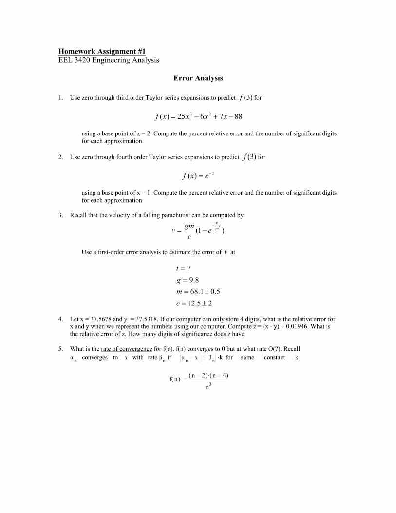
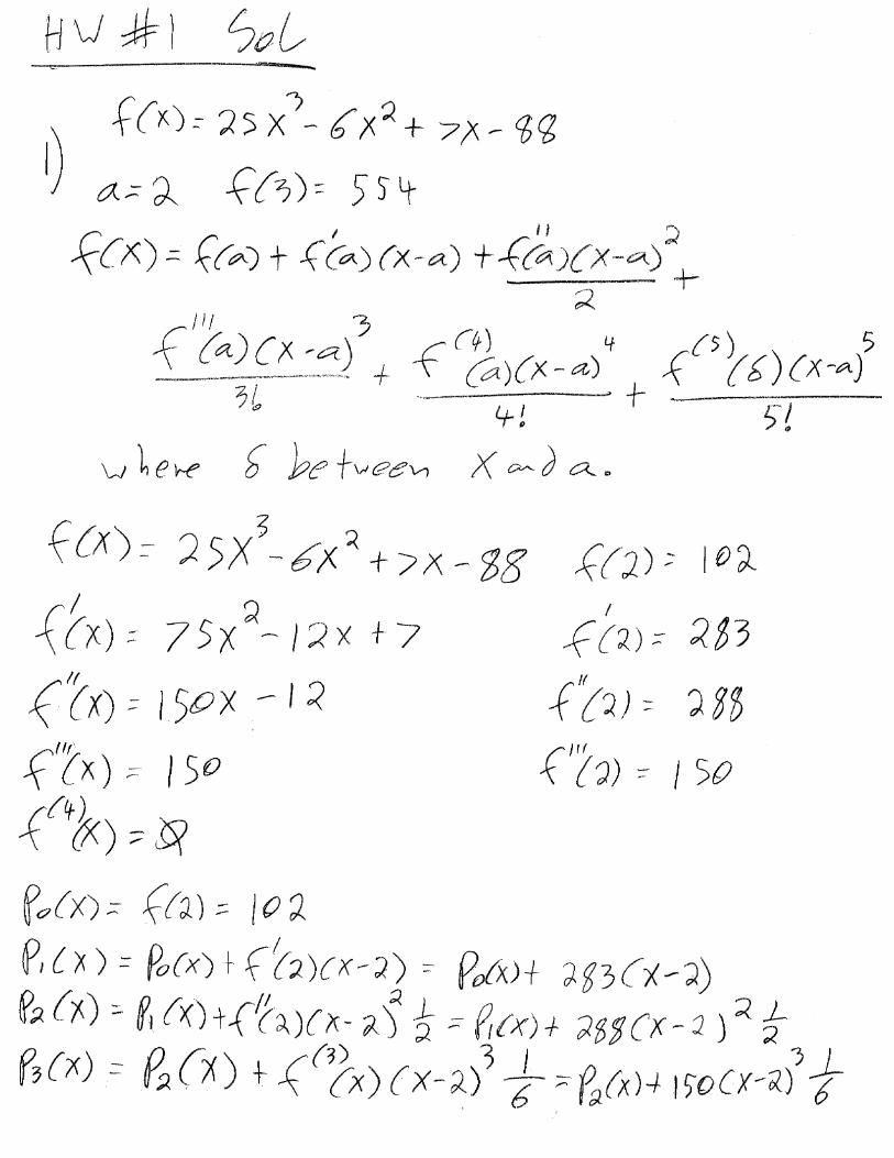
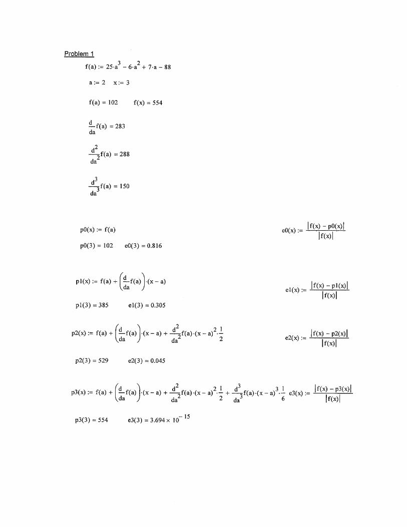
1. Use zero through third order Taylor series expansions to predict )3(f for

887625)( 23 −+−= xxxxf

using a base point of x = 2. Compute the percent relative error and the number of significant digits for each approximation.

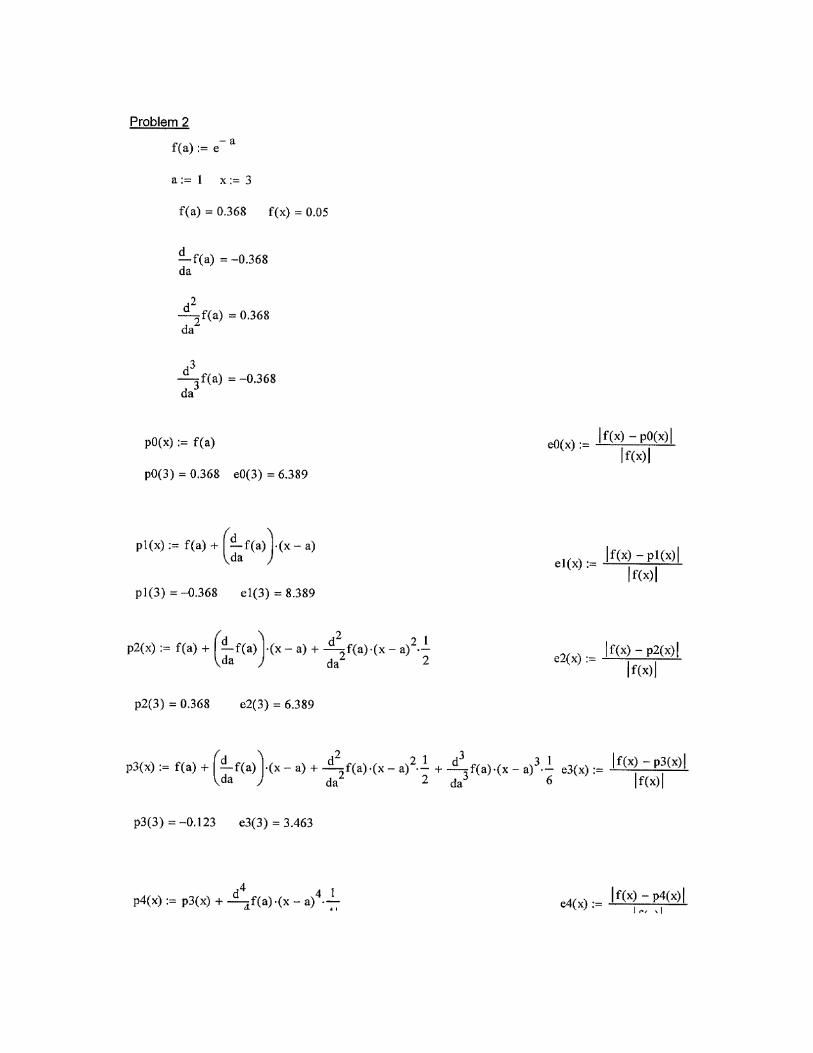
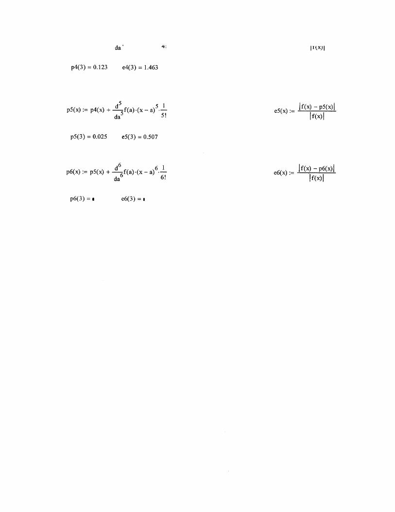
2. Use zero through fourth order Taylor series expansions to predict )3(f for

xexf −=)(

using a base point of x = 1. Compute the percent relative error and the number of significant digits for each approximation.

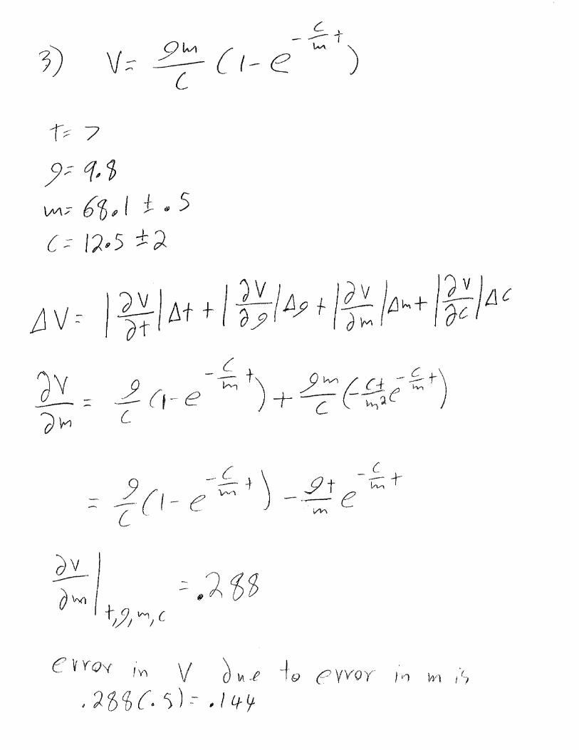
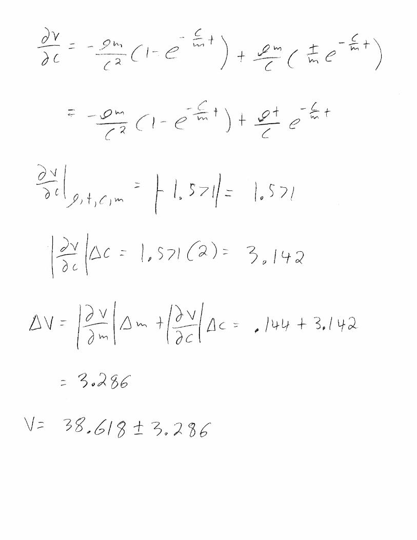
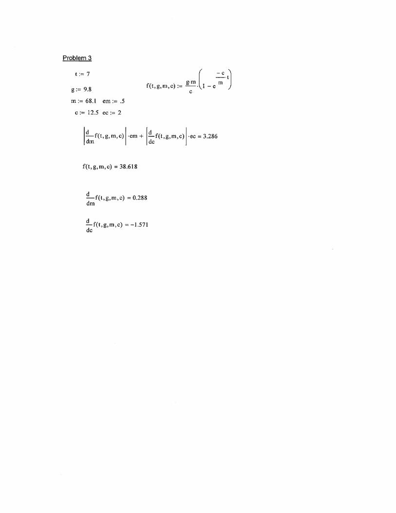
3. Recall that the velocity of a falling parachutist can be computed by

)1(t

mc

ecgmv

−−=

Use a first-order error analysis to estimate the error of v at

25.125.01.68

8.97

±=±=

==

cmgt

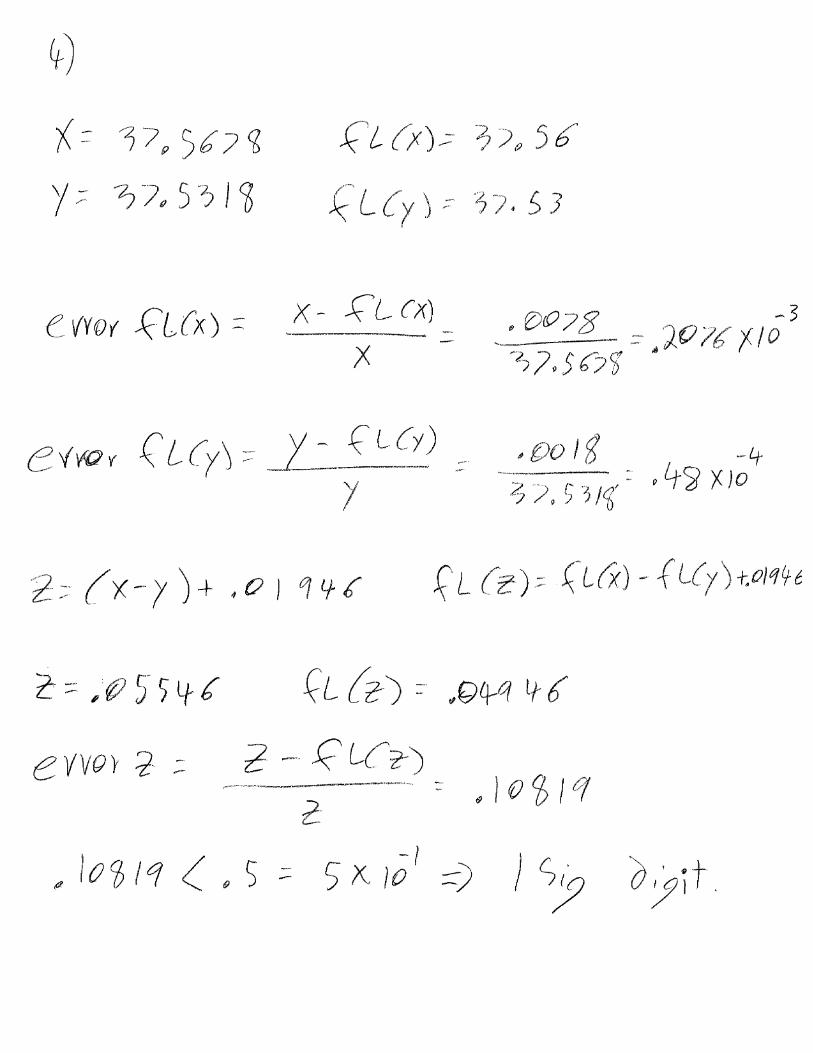
4. Let x = 37.5678 and y = 37.5318. If our computer can only store 4 digits, what is the relative error for

x and y when we represent the numbers using our computer. Compute z = (x - y) + 0.01946. What is the relative error of z. How many digits of significance does z have.

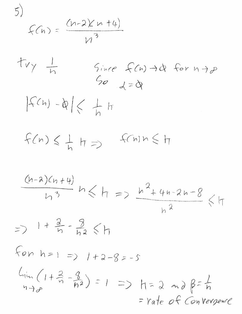
5. What is the rate of convergence for f(n). f(n) converges to 0 but at what rate O(?). Recall

α n converges to α with rate β n if α n α .β n k for some constant k

f( )n

.( )n 2 ( )n 4

n3

Homework Assignment #2 EEL 3420 Engineering Analysis

Root Finding Techniques

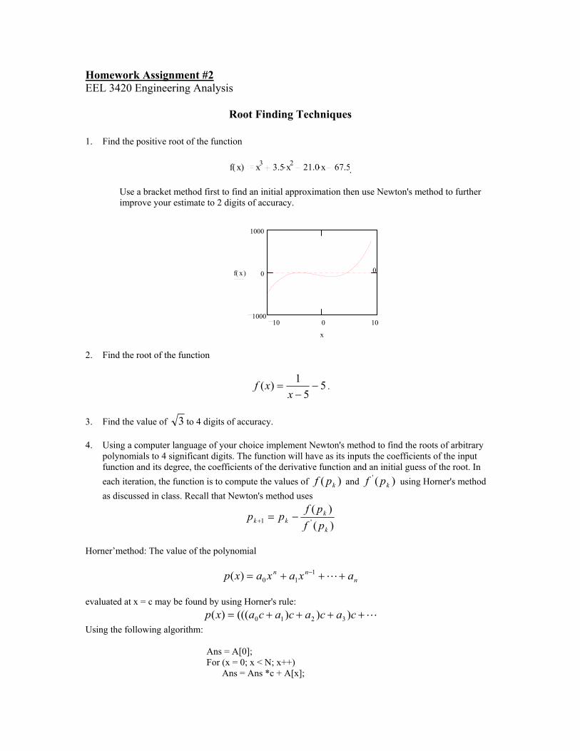
1. Find the positive root of the function

f( )x x3 .3.5 x2 .21.0 x 67.5.

Use a bracket method first to find an initial approximation then use Newton's method to further improve your estimate to 2 digits of accuracy.

1000

0

1000

10 0 10

0f( )x

x 2. Find the root of the function

55

1)( −−

=x

xf .

3. Find the value of 3 to 4 digits of accuracy. 4. Using a computer language of your choice implement Newton's method to find the roots of arbitrary

polynomials to 4 significant digits. The function will have as its inputs the coefficients of the input function and its degree, the coefficients of the derivative function and an initial guess of the root. In each iteration, the function is to compute the values of )( kpf and )(' kpf using Horner's method as discussed in class. Recall that Newton's method uses

)()(

'1k

kkk pf

pfpp −=+

Horner’method: The value of the polynomial

nnn axaxaxp +++= − L1

10)( evaluated at x = c may be found by using Horner's rule:

L++++= cacacacaxp )))((()( 3210 Using the following algorithm:

Ans = A[0]; For (x = 0; x < N; x++) Ans = Ans *c + A[x];

Homework Assignment #3 EEL 3420 Engineering Analysis

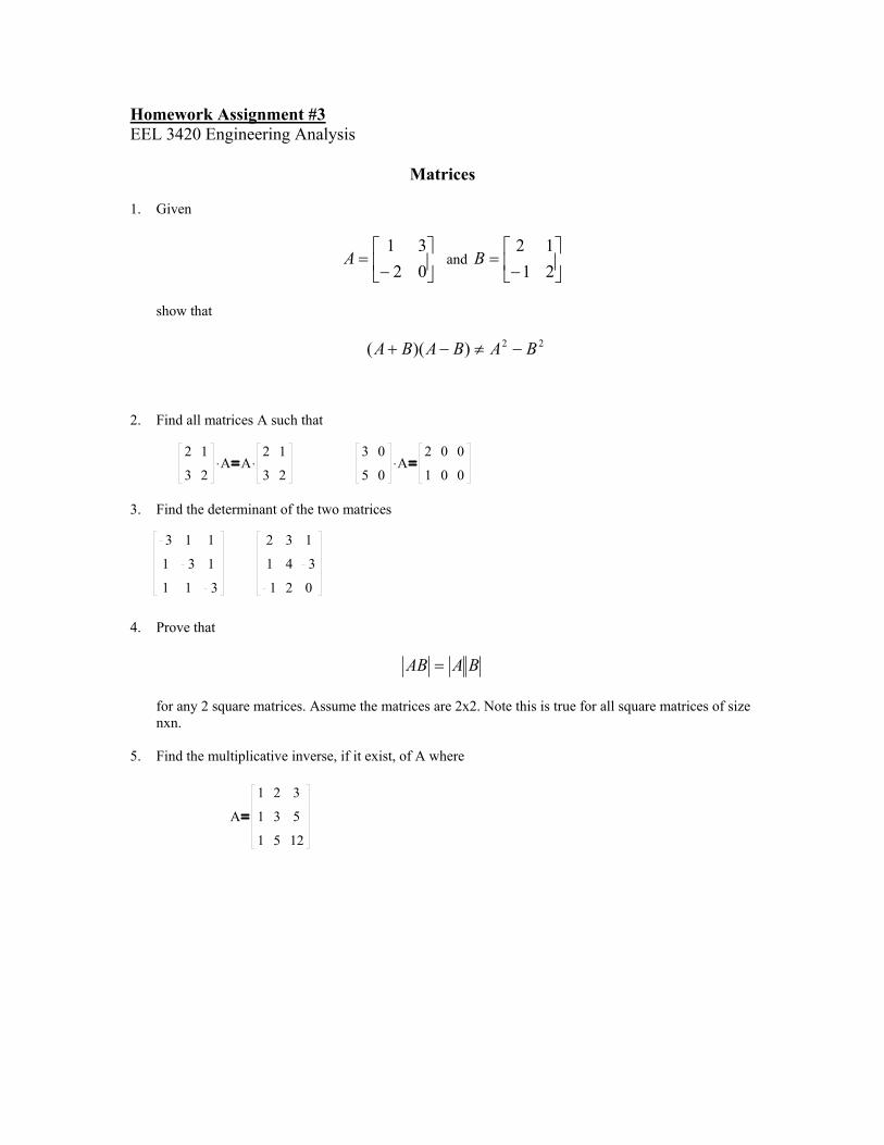
Matrices 1. Given

−

=0231

A and

−

=2112

B

show that

22))(( BABABA −≠−+

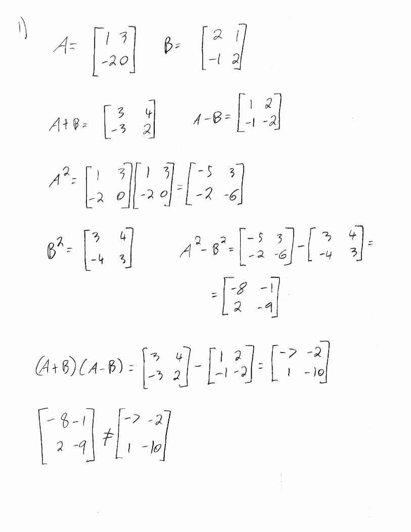
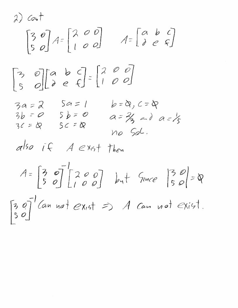
2. Find all matrices A such that

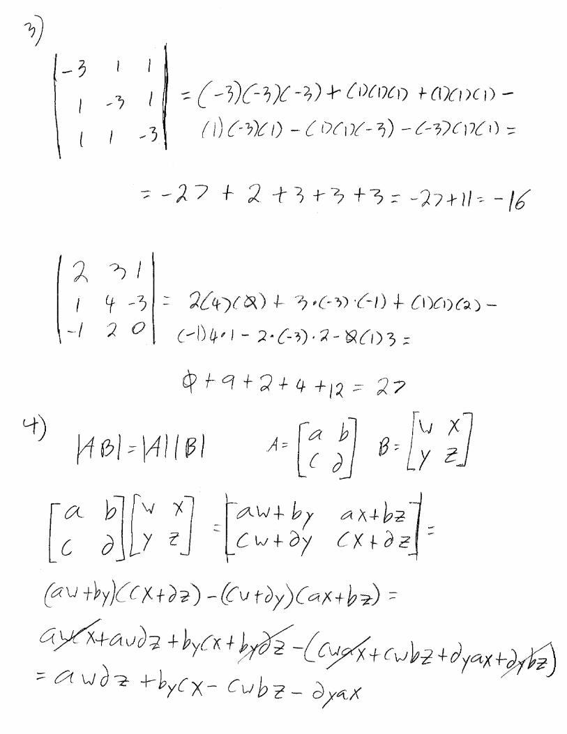
3. Find the determinant of the two matrices

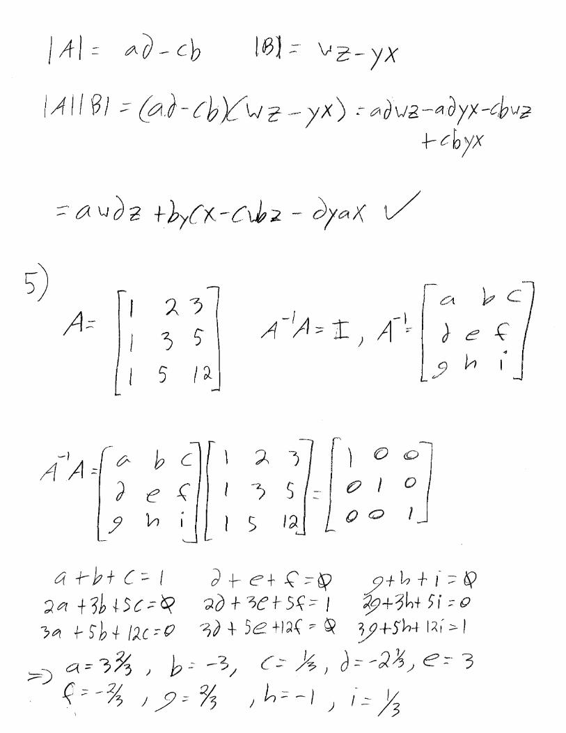
4. Prove that

BAAB =

for any 2 square matrices. Assume the matrices are 2x2. Note this is true for all square matrices of size nxn.

5. Find the multiplicative inverse, if it exist, of A where

3

5

0

0A.

2

1

0

0

0

0

2

3

1

2A. A

2

3

1

2.

3

1

1

1

3

1

1

1

3

2

1

1

3

4

2

1

3

0

A

1

1

1

2

3

5

3

5

12

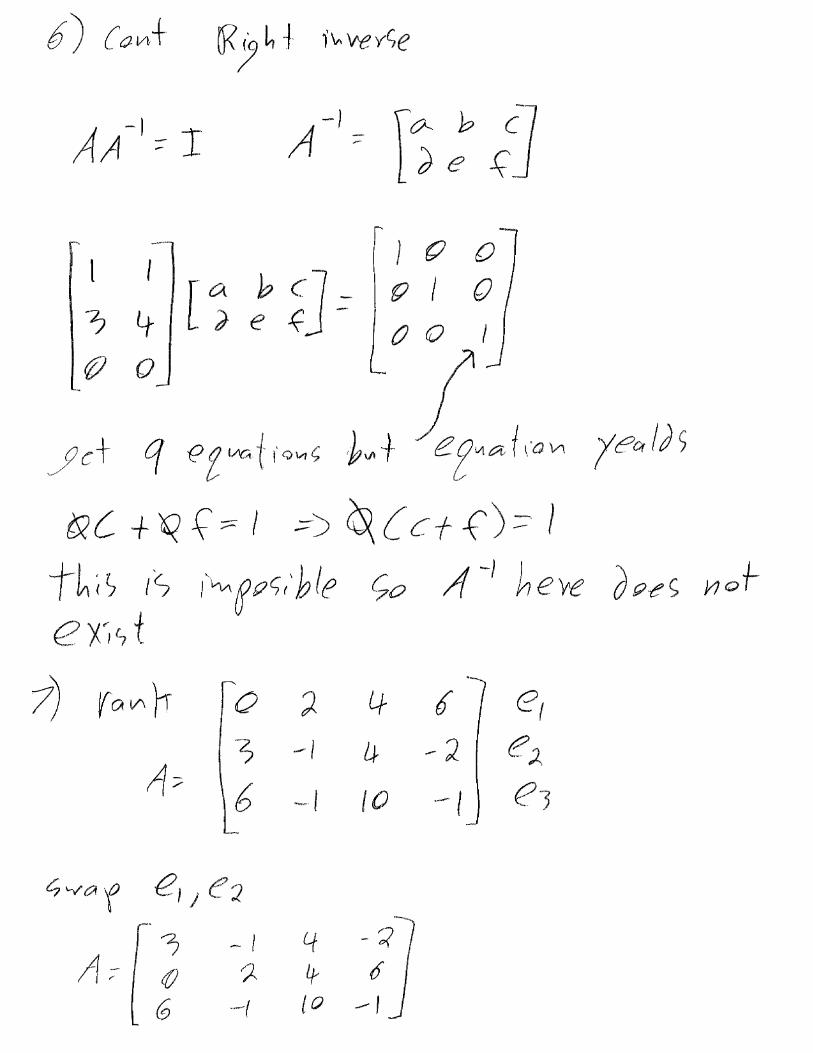
6. Find the left multiplicative inverse, if it exist, of

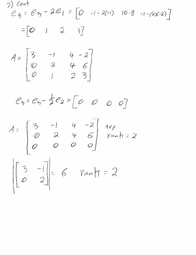
Show that the right inverse does not exist. 7. Determine the rank of the following matrix.

Use the 3 elementary row transformations to simplify the work.

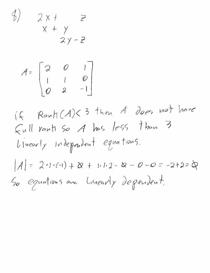
8. Show that the following 3 equations are linearly dependant:

zyyxzx

−++

2

2

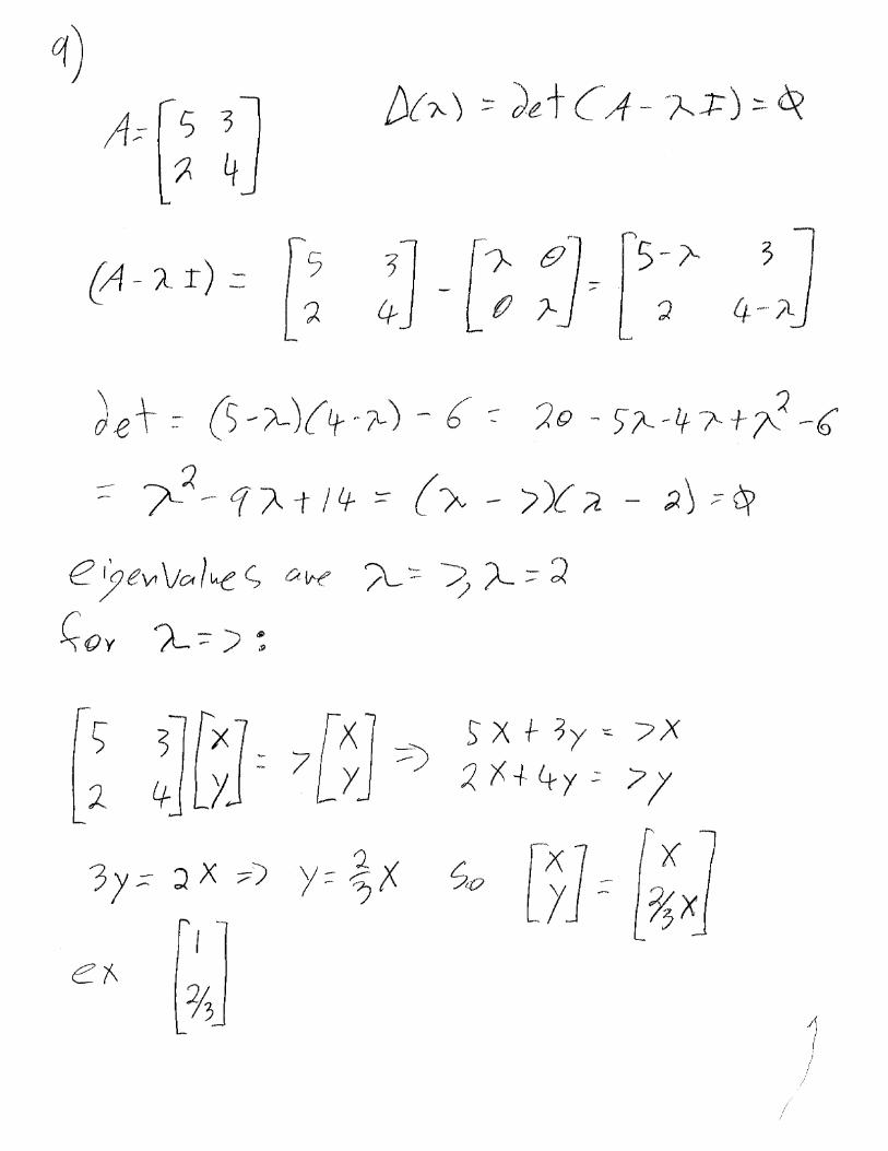
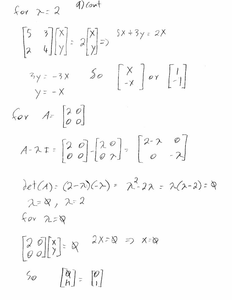
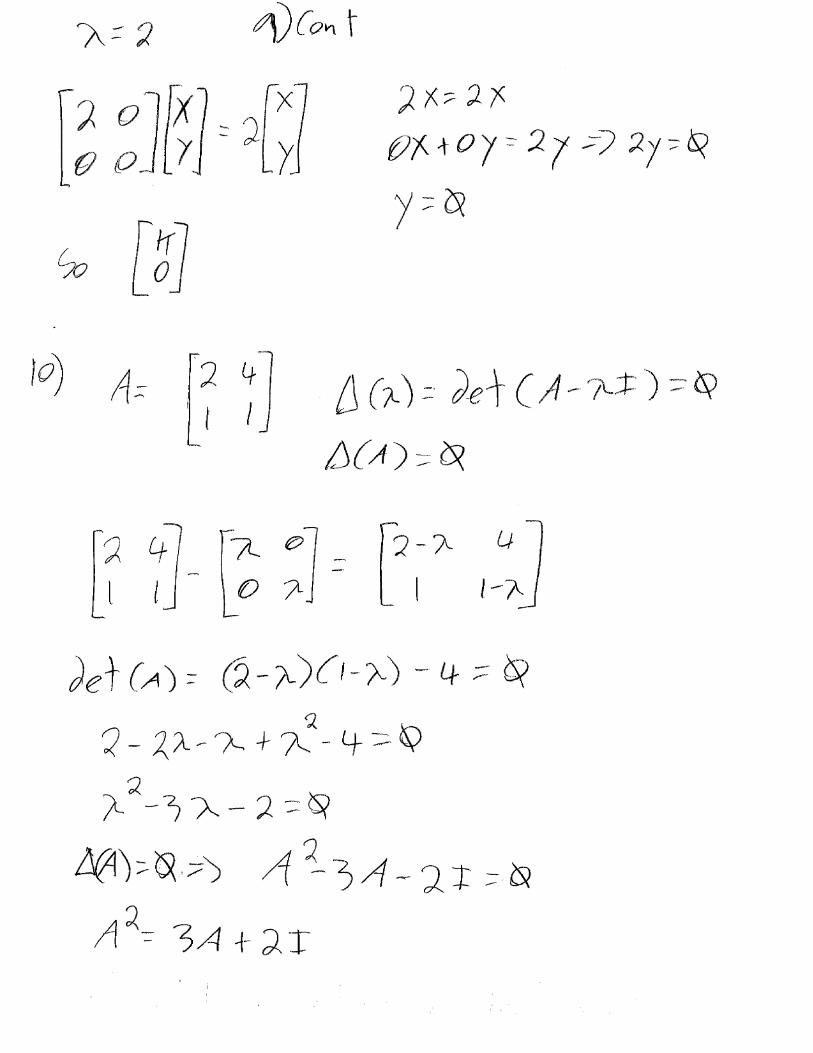
9. Find the characteristic equation, the eigenvalues, and a set of eigenvectors for the given 4 matrices.

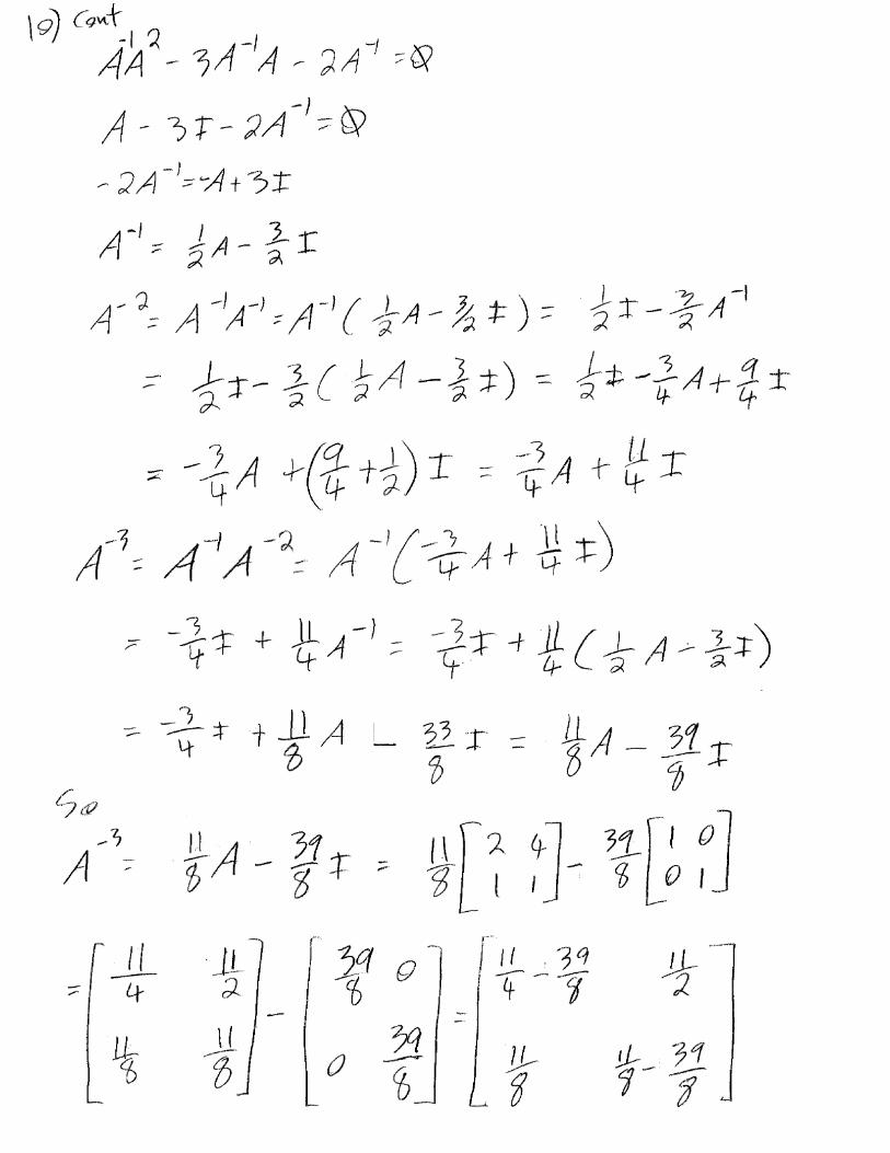
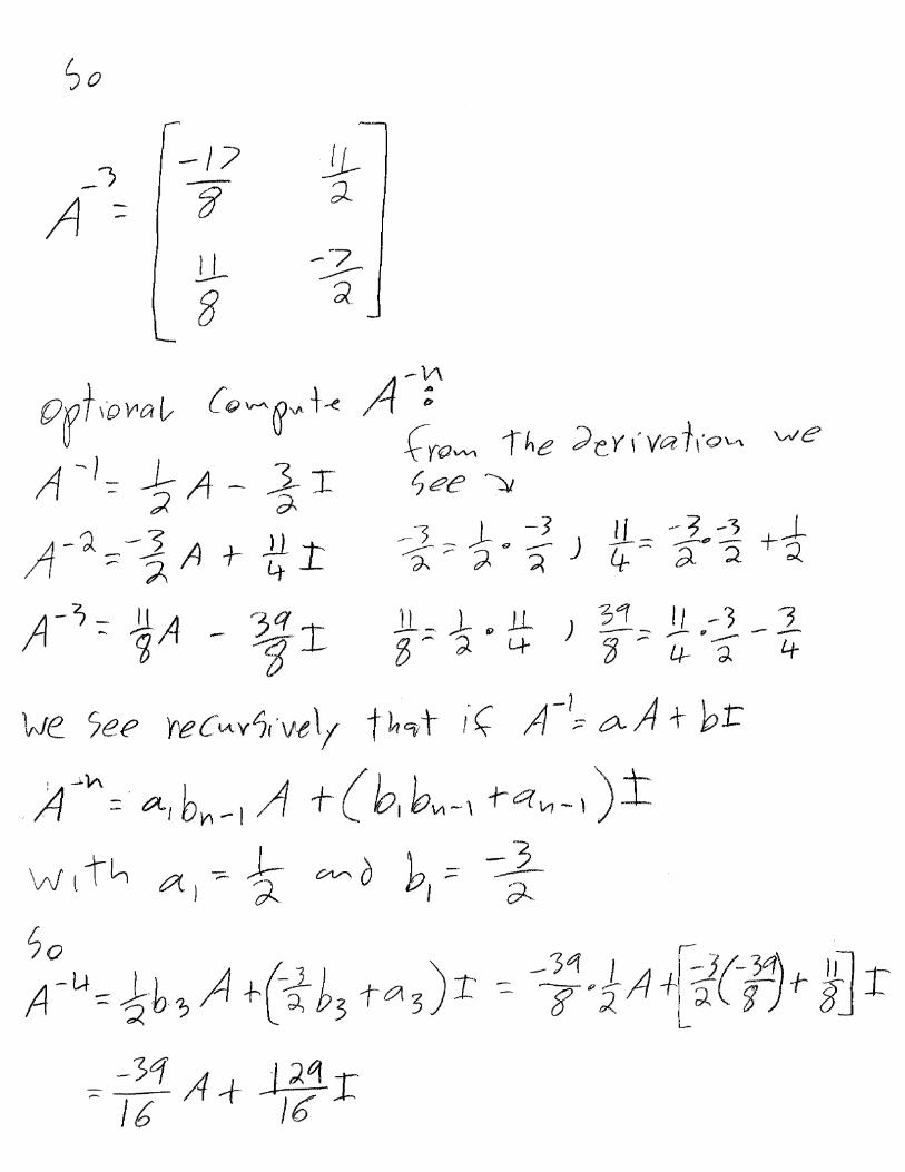
10. Use the Hamilton-Cayley theorem to find

for the matrix

1

3

0

1

4

0

0

3

6

2

1

1

4

4

10

6

2

1

5

2

3

4

1

4

2

3,

2

0

0

0,

3

0

2

0

1

2

2

2

2

,

A 3

A2

1

4

1

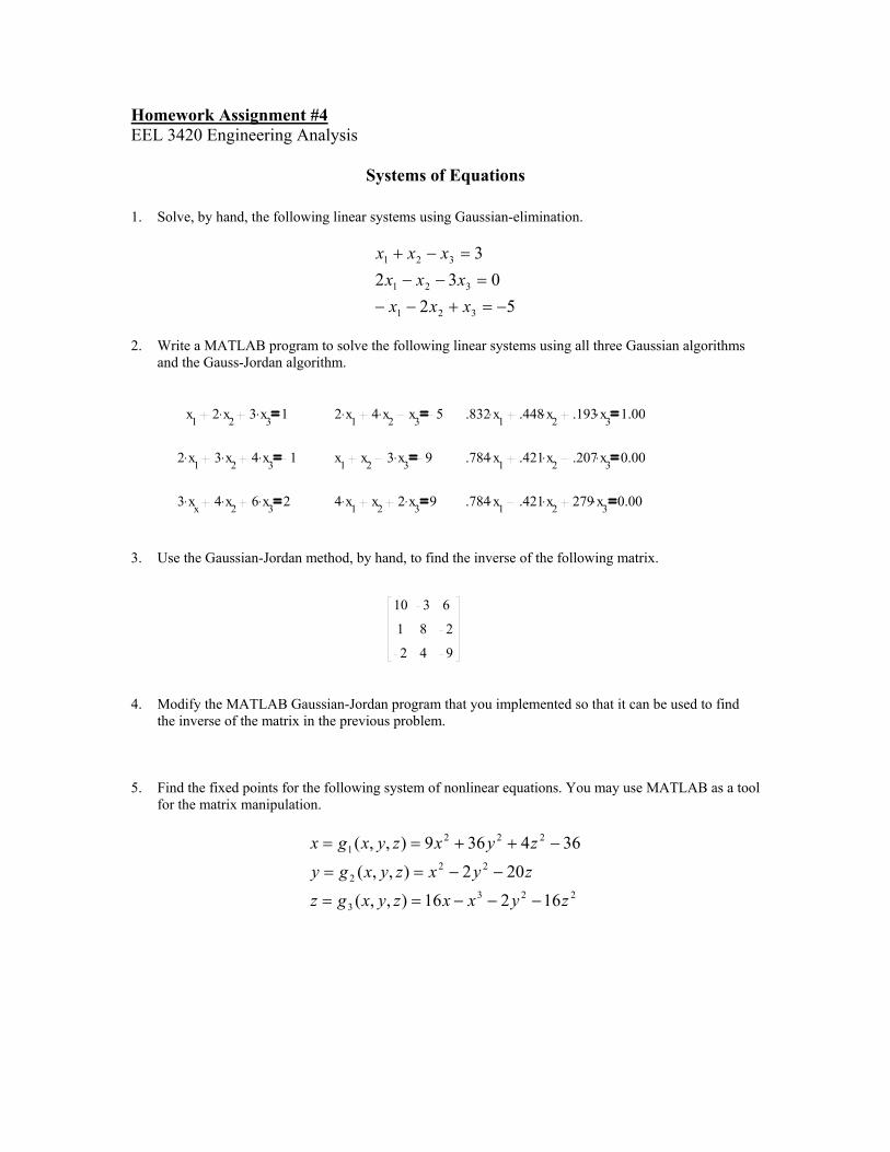
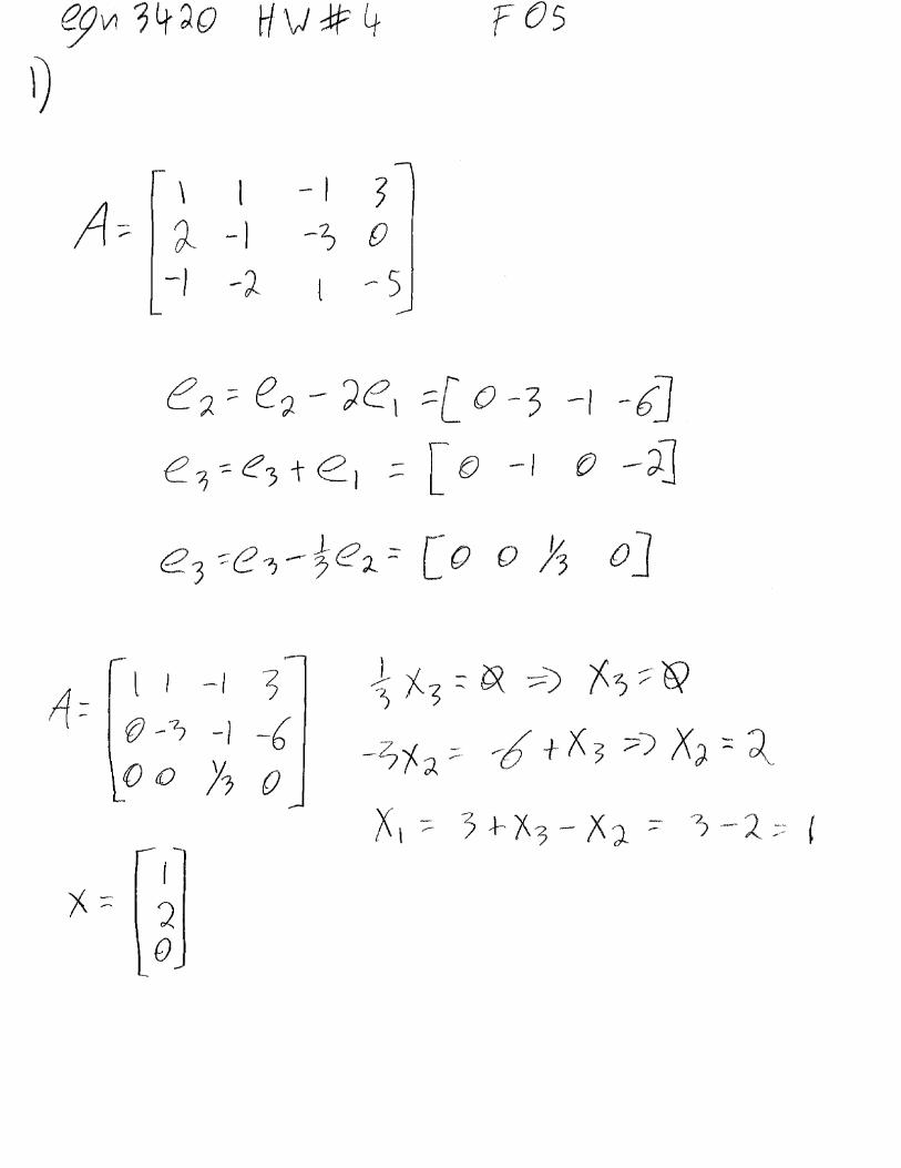
Homework Assignment #4 EEL 3420 Engineering Analysis

Systems of Equations

1. Solve, by hand, the following linear systems using Gaussian-elimination.

52032

3

321

321

321

−=+−−=−−

=−+

xxxxxx

xxx

2. Write a MATLAB program to solve the following linear systems using all three Gaussian algorithms

and the Gauss-Jordan algorithm.

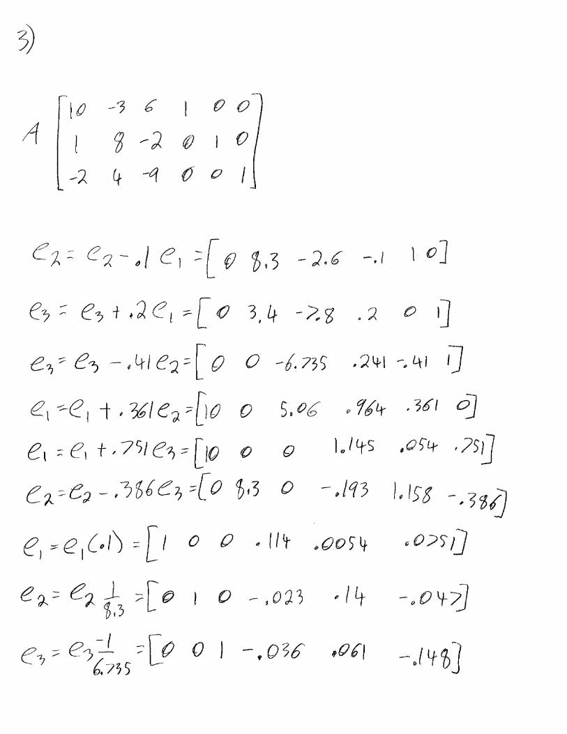
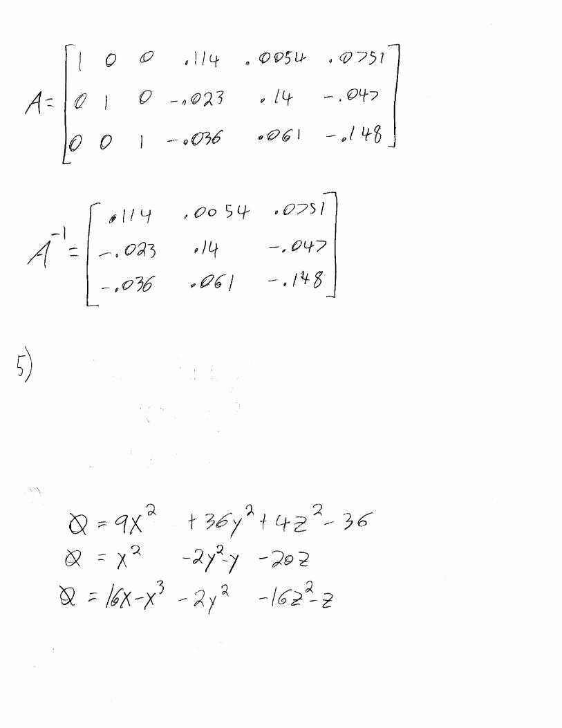
3. Use the Gaussian-Jordan method, by hand, to find the inverse of the following matrix.

4. Modify the MATLAB Gaussian-Jordan program that you implemented so that it can be used to find

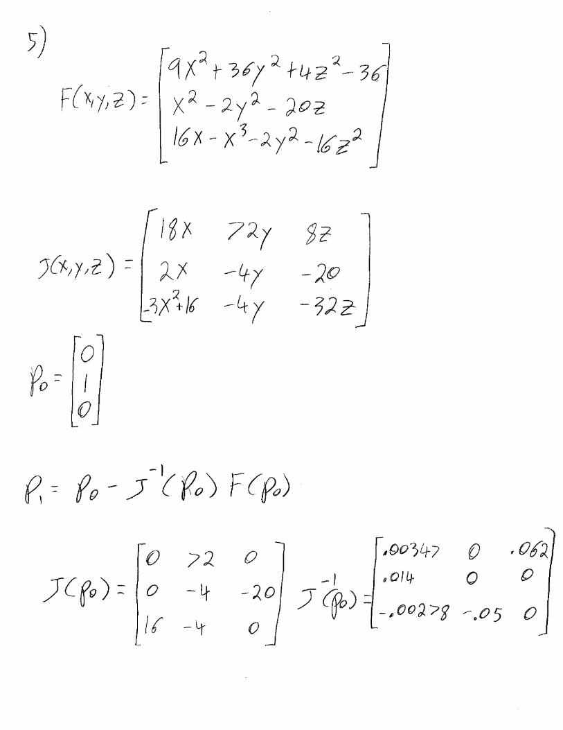
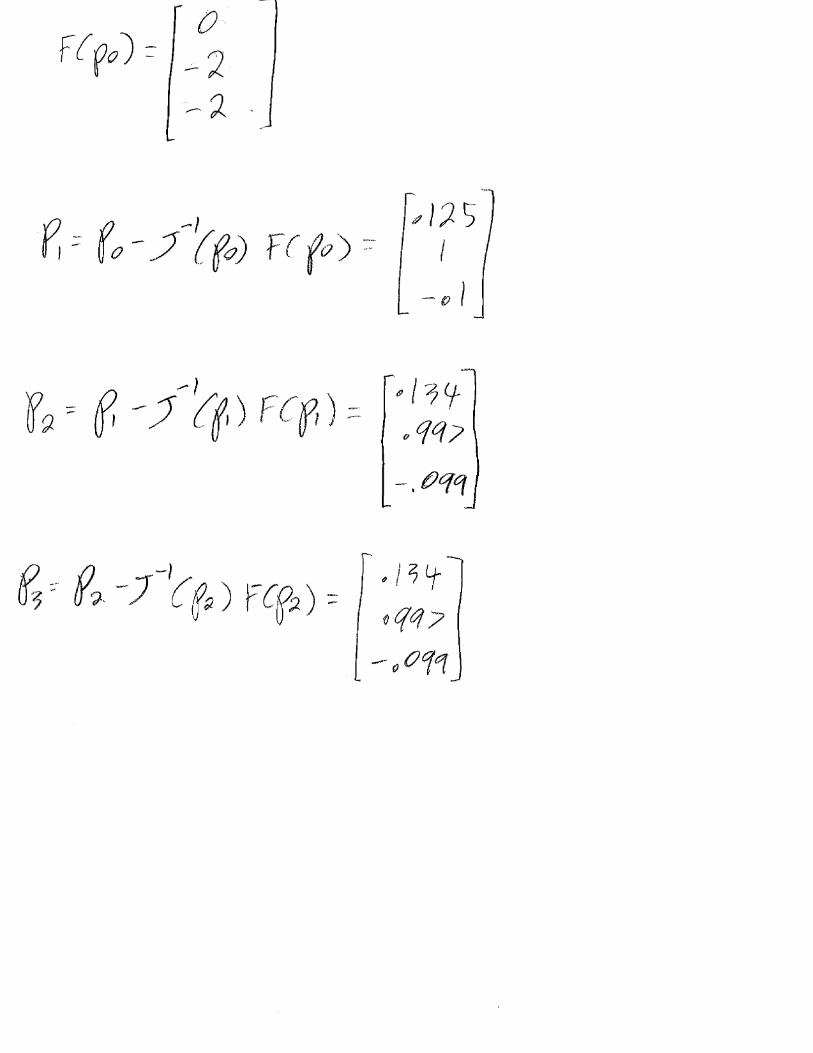
the inverse of the matrix in the previous problem. 5. Find the fixed points for the following system of nonlinear equations. You may use MATLAB as a tool

for the matrix manipulation.

2233

222

2221

16216),,(

202),,(

364369),,(

zyxxzyxgzzyxzyxgyzyxzyxgx

−−−==

−−==

−++==

x1 2 x2. 3 x3

. 1 2 x1. 4 x2

. x3 5 .832 x1. .448 x2

. .193 x3. 1.00

2 x1. 3 x2

. 4 x3. 1 x1 x2 3 x3

. 9 .784 x1. .421 x2

. .207 x3. 0.00

3 xx. 4 x2

. 6 x3. 2 4 x1

. x2 2 x3. 9 .784 x1

. .421 x2. 279 x3

. 0.00

10

1

2

3

8

4

6

2

9

Homework Assignment #5 EEL 3420 Engineering Analysis

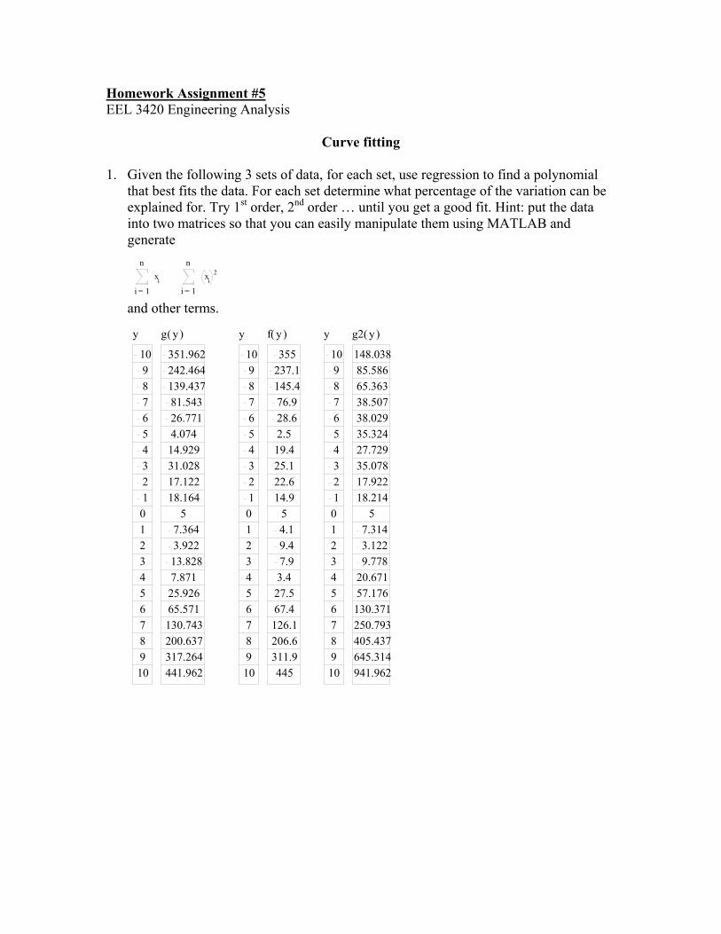
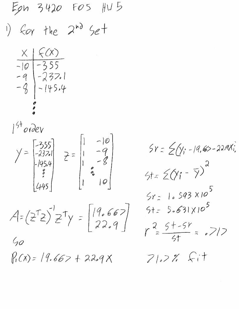
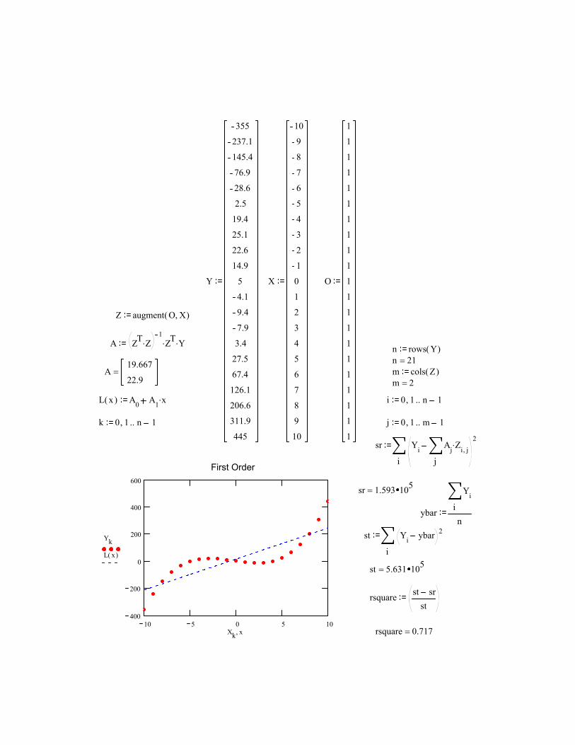
Curve fitting 1. Given the following 3 sets of data, for each set, use regression to find a polynomial

that best fits the data. For each set determine what percentage of the variation can be explained for. Try 1st order, 2nd order … until you get a good fit. Hint: put the data into two matrices so that you can easily manipulate them using MATLAB and generate

and other terms.

1

n

i

xi

= 1

n

i

xi2

=

y

10987654321012345678910

g y( )

351.962242.464139.43781.54326.7714.07414.92931.02817.12218.164

57.3643.92213.8287.87125.92665.571130.743200.637317.264441.962

y

10987654321012345678910

f y( )

355237.1145.476.928.62.519.425.122.614.9

54.19.47.93.427.567.4126.1206.6311.9445

y

10987654321012345678910

g2 y( )

148.03885.58665.36338.50738.02935.32427.72935.07817.92218.214

57.3143.1229.778

20.67157.176130.371250.793405.437645.314941.962

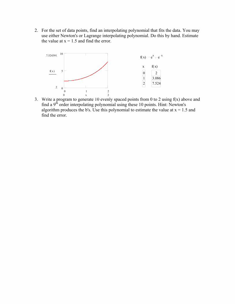
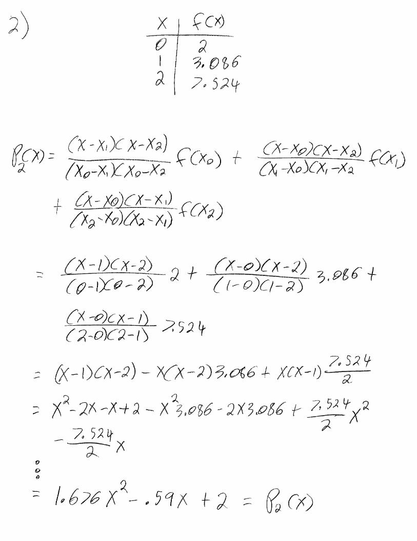
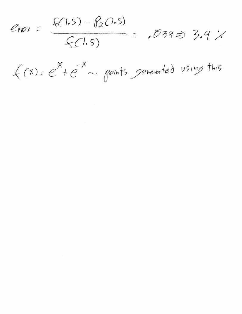
2. For the set of data points, find an interpolating polynomial that fits the data. You may use either Newton's or Lagrange interpolating polynomial. Do this by hand. Estimate the value at x = 1.5 and find the error.

3. Write a program to generate 10 evenly spaced points from 0 to 2 using f(x) above and find a 9th order interpolating polynomial using these 10 points. Hint: Newton's algorithm produces the b's. Use this polynomial to estimate the value at x = 1.5 and find the error.

f x( ) ex e x

x

012

f x( )

23.0867.524

7.524391

2

f x( )

20 x0 1 2

0

5

10

Y

355

237.1

145.4

76.9

28.6

2.5

19.4

25.1

22.6

14.9

5

4.1

9.4

7.9

3.4

27.5

67.4

126.1

206.6

311.9

445

X

10

9

8

7

6

5

4

3

2

1

0

1

2

3

4

5

6

7

8

9

10

O

1

1

1

1

1

1

1

1

1

1

1

1

1

1

1

1

1

1

1

1

1

Z augment O X,( )

A ZT Z.1ZT. Y. n rows Y( )

n 21=A

19.667

22.9= m cols Z( )

m 2=

L x( ) A0 A1 x. i 0 1, n 1..

k 0 1, n 1.. j 0 1, m 1..

sr

i

Yij

Aj Zi j,. 2

Yk

L x( )

Xk x,10 5 0 5 10

400

200

0

200

400

600

First Order

sr 1.593 105=

ybar i

Yi

nst

i

Yi ybar 2

st 5.631 105=

rsquare st srst

rsquare 0.717=

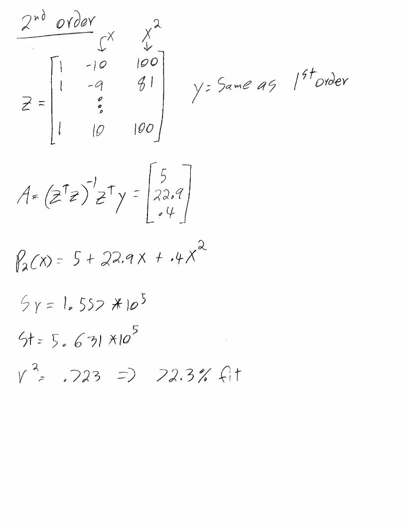
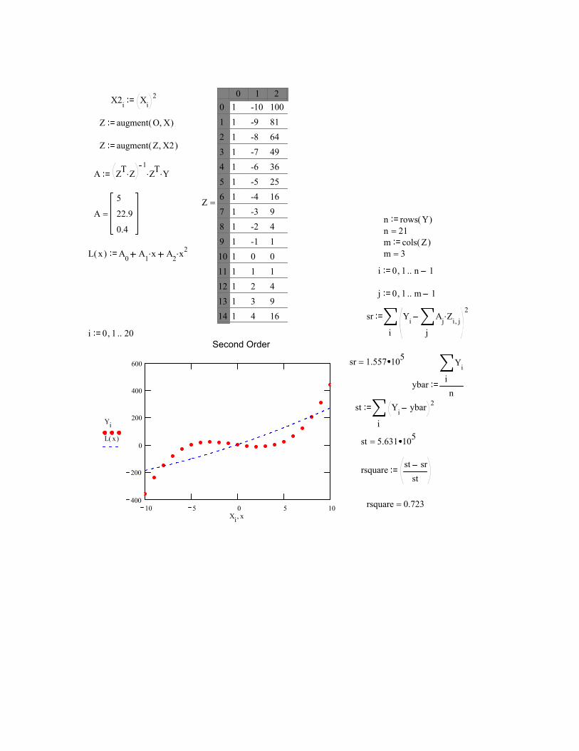
X2i Xi2

Z augment O X,( )

Z augment Z X2,( )

A ZT Z.1ZT. Y.

Z

0 1 201234567891011121314

1 -10 1001 -9 811 -8 641 -7 491 -6 361 -5 251 -4 161 -3 91 -2 41 -1 11 0 01 1 11 2 41 3 91 4 16

=A

5

22.9

0.4

= n rows Y( )n 21=m cols Z( )

L x( ) A0 A1 x. A2 x

2. m 3=

i 0 1, n 1..

j 0 1, m 1..

sr

i

Yij

Aj Zi j,. 2

i 0 1, 20..Second Order

Yi

L x( )

Xi x,10 5 0 5 10

400

200

0

200

400

600 sr 1.557 105=

ybar i

Yi

nst

i

Yi ybar 2

st 5.631 105=

rsquare st srst

rsquare 0.723=

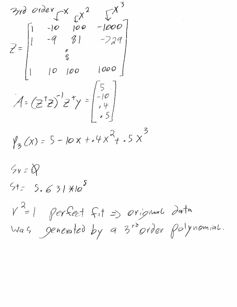
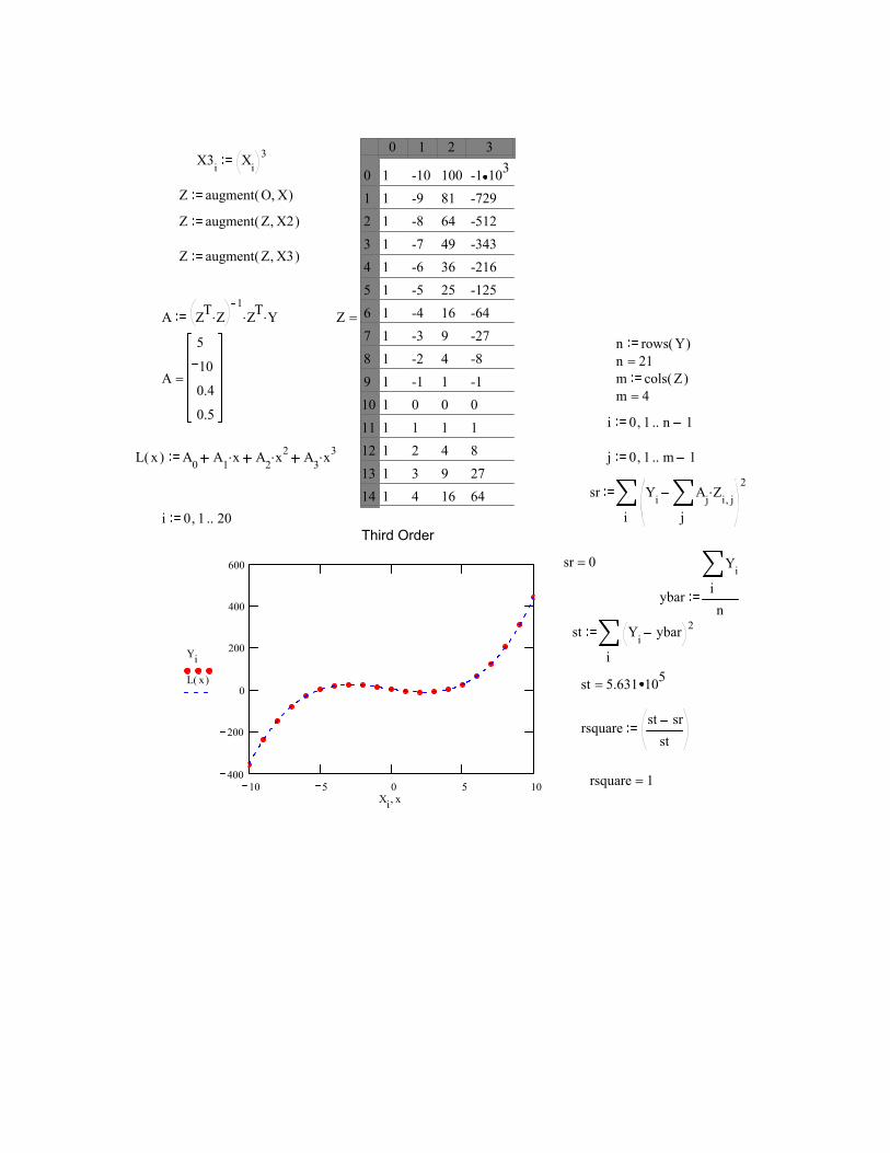
X3i Xi3

Z augment O X,( )

Z augment Z X2,( )

Z augment Z X3,( )

A ZT Z.1ZT. Y. Z

0 1 2 3

01234567891011121314

1 -10 100 -1 103

1 -9 81 -7291 -8 64 -5121 -7 49 -3431 -6 36 -2161 -5 25 -1251 -4 16 -641 -3 9 -271 -2 4 -81 -1 1 -11 0 0 01 1 1 11 2 4 81 3 9 271 4 16 64

=

n rows Y( )n 21=

A

5

10

0.4

0.5

= m cols Z( )m 4=

i 0 1, n 1..

L x( ) A0 A1 x. A2 x

2. A3 x3. j 0 1, m 1..

sr

i

Yij

Aj Zi j,. 2

i 0 1, 20..Third Order

Yi

L x( )

Xi x,10 5 0 5 10

400

200

0

200

400

600 sr 0=

ybar i

Yi

nst

i

Yi ybar 2

st 5.631 105=

rsquare st srst

rsquare 1=

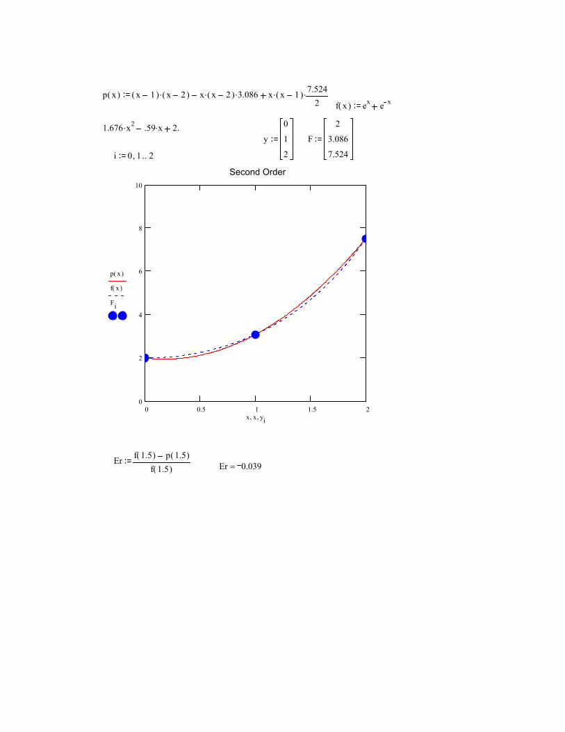
p x( ) x 1( ) x 2( ). x x 2( ). 3.086. x x 1( ). 7.5242

.f x( ) ex e x

1.676 x2. .59 x. 2.y

0

1

2

F

2

3.086

7.524i 0 1, 2..

p x( )

f x( )

Fi

x x, yi,0 0.5 1 1.5 2

0

2

4

6

8

10

Second Order

Er f 1.5( ) p 1.5( )f 1.5( ) Er 0.039=

Homework Assignment #6 EEL 3420 Engineering Analysis

Numerical Integration, Differentiation, and Differential Equations

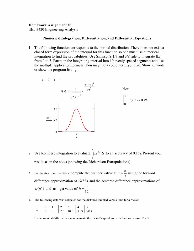
1. The following function corresponds to the normal distribution. There does not exist a closed form expression of the integral for this function so one must use numerical integration to find the probabilities. Use Simpson's 1/3 and 3/8 rule to integrate f(x) from 0 to 3. Partition the integrating interval into 10 evenly spaced segments and use the multiple application formula. You may use a computer if you like. Show all work or show the program listing.

2. Use Romberg integration to evaluate ∫4

0

2 dxxe x to an accuracy of 0.1%. Present your

results as in the notes (showing the Richardson Extrapolations).

3. For the function xy sin= compute the first derivative at 3π

=x using the forward

difference approximation of )( 2hO and the centered difference approximations of

)( 4hO and using a value of 12π

=h .

4. The following data was collected for the distance traveled versus time for a rocket.

T 0 1 2 3 4 5 Y 0 2.1 7.8 18.2 31.9 50.3

Use numerical differentiation to estimate the rocket’s speed and acceleration at time T = 3.

µ 0 σ 1

f x( ) 1

2 π. σ2.

e

x µ( )2

2 σ2..

f x( )

x0

0

0.2

0.4

Note

0

3xf x( ) d 0.499=